correcting the errors: volatility forecast ... - github pages

Correcting the Errors:Volatility Forecast Evaluation Using

High-Frequency Data and Realized Volatilities∗

Torben G. Andersen†, Tim Bollerslev‡, and Nour Meddahi§

First Draft: September 2002This Draft: November 5, 2003

Abstract

We develop general model-free adjustment procedures for the calculation of unbiased

volatility loss functions based on practically feasible realized volatility benchmarks. The

procedures, which exploit the recent non-parametric asymptotic distributional results in

Barndorff-Nielsen and Shephard (2002a, 2003a) along with new results explicitly allowing

for leverage effects, are both easy-to-implement and highly accurate in empirically realistic

situations. On properly accounting for the measurement errors in the volatility forecast

evaluations reported in Andersen, Bollerslev, Diebold and Labys (2003), the adjustments

result in markedly higher estimates for the true degree of return-volatility predictability.

∗This work was supported by a grant from the National Science Foundation to the NBER (Andersen andBollerslev), and from FQRSC, IFM2, MITACS, NSERC, SSHRC, and Jean-Marie Dufour’s EconometricsChair of Canada (Meddahi). Some of this material was circulated earlier as part of the paper “AnalyticalEvaluation of Volatility Forecasts.” Detailed comments by Neil Shephard, Tom McCurdy, two anonymousreferees, and the editor (Costas Meghir) have importantly improved the paper. We would also like to thankFrancis X. Diebold for many discussions on closely related ideas, as well as seminar participants at the 2002NBER/NSF Time Series Conference and the 2003 CIRANO-CIREQ Financial Econometrics Conference.The third author thanks the Bendheim Center for Finance at Princeton University for its hospitality duringhis visit where part of the research was done.

†Department of Finance, Kellogg School of Management, Northwestern University, Evanston, IL 60208,and NBER, USA, phone: 847-467-1285, e-mail: [email protected].

‡Department of Economics, Duke University, Durham, NC 27708, and NBER, USA, phone: 919-660-1846,e-mail: [email protected].

§Departement de sciences economiques, CIRANO, CIREQ, Universite de Montreal, C.P. 6128,succursale Centre-ville, Montreal (Quebec), H3C 3J7, Canada, phone: 514-343-2399, e-mail:[email protected]; web-page: http://www.mapageweb.umontreal.ca/meddahin/.

“ARCH models have become indispensable tools not only for researchers, but also for analysts onfinancial markets, who use them in asset pricing and in evaluating portfolio risk.” Press release,October 8, 2003: The Bank of Sweden Prize in Economic Sciences in Memory of Alfred Nobel.

1 Introduction

The burgeoning literature on time-varying financial market volatility is abound with

empirical studies in which competing models are evaluated and compared on the basis of

their forecast performance. Contrary to the typical setting for economic forecast evaluation,

the variable of interest in that context - the volatility - is not directly observable but

rather inherently latent. Consequently, any ex-post assessment of forecast precision must

contend with a fundamental errors-in-variable problem associated with the measurement of

the realization of the forecasted variable. Growing recognition of the importance of this

issue has led a number of recent studies to advocate the use of so-called realized volatilities,

constructed from the summation of finely sampled squared high-frequency returns, as a

practical method for improving the ex-post volatility measures.

The use of realized volatility as the practical benchmark may be justified by standard

continuous-time arguments. Assuming that the sampling frequency of the squared returns

utilized in the realized volatility computations approaches zero, the realized volatility

consistently estimates the true (latent) integrated volatility under quite general conditions,

where importantly, the latter concept corresponds to the realization of the (cumulative)

instantaneous variance process over the relevant horizon (see, e.g., Andersen and Bollerslev,

1998; Andersen, Bollerslev, Diebold and Labys, 2001; Barndorff-Nielsen and Shephard,

2001, 2002a,b; Comte and Renault, 1998; along with the recent survey by Andersen,

Bollerslev and Diebold, 2003). Unfortunately, market microstructure frictions distort the

measurement of returns at the highest frequencies so that, e.g., tick-by-tick return processes

blatantly violate the theoretical semi-martingale restrictions implied by the no-arbitrage

assumptions in continuous-time asset pricing models. These same features also bias empirical

realized volatility measures constructed directly from the ultra high-frequency returns, so in

practice the measures are instead typically constructed from intraday returns sampled at an

intermediate frequency.1 As such, the integrated volatility is invariably measured with error

(see, e.g., the numerical calculations in Andreou and Ghysels, 2002, and Bai, Russell, and

Tiao, 2000). The exact form of the measurement error will, of course, depend on the assumed

model structure (see, e.g., Meddahi, 2002, and Barndorff-Nielsen and Shephard, 2002a), but

it will generally result in a downward bias in the estimated degree of predictability obtained

1For instance, the daily realized volatilities in Andersen, Bollerslev, Diebold and Labys (2003) (henceforthABDL (2003)) discussed further below are based on the summation of squared half-hourly foreign exchangerate returns, but either 5-minute or 15-minute returns are other common choices in the literature.

1

through any forecast evaluation criterion that simply uses the realized volatility in place

of the true (latent) integrated volatility. Although this bias may be large (Andersen and

Bollerslev, 1998), it is almost always ignored in empirical applications.

This note addresses that issue by developing general model-free adjustment procedures

that allow for the calculation of simple unbiased loss functions in realistic forecast

situations. Moreover, the adjustments are simple to implement in practice. The derivation

exploits the recent asymptotic (for increasing sampling frequency) distributional results in

Barndorff-Nielsen and Shephard (2002a). While these results explicitly rules out so-called

leverage effects, we show that the same approximate adjustment procedures apply in the

context of the general eigenfunction stochastic volatility class of models pioneered by

Meddahi (2001) explicitly allowing for non-zero contemporaneous correlations between the

separate shocks in the return and volatility processes. Following Andersen and Bollerslev

(1998) and ABDL (2003), we focus our forecast comparisons on the value of the coefficient of

multiple correlation, or R2, in the Mincer-Zarnowitz style regressions of the ex-post realized

volatility on the corresponding model forecasts,2 but our procedures are general and could

be applied in the adjustment of other loss functions used in the evaluation of any arbitrary

set of volatility forecasts. On applying the procedures in the context of ABDL (2003), we

obtain markedly higher estimates for the true degree of return-volatility predictability, with

the adjusted R2’s exceeding their unadjusted counterparts by up to forty-percent.

We proceed as follows. The first subsection below introduces the notions of integrated and

realized volatility, along with the (feasible) asymptotic distribution theory due to Barndorff-

Nielsen and Shephard (2002a). The development of the practical and easy-to-implement

adjustment procedures based on this theory is then presented in the next subsection,

followed by our new theoretical results explicitly allowing for leverage effects. Utilizing

these results, the last section provides a reassessment of the empirical evidence in ABDL

(2003) related to the fit of the Mincer-Zarnowitz style volatility regressions. The accuracy

of the asymptotic approximations - which form the basis for our approach - is confirmed

through Monte Carlo simulations for models calibrated to reflect empirically relevant and

challenging specifications. The details of the simulations and all of the technical proofs are

deferred to two Appendixes.

2 Theory

We focus on a single asset traded in a liquid financial market. Assuming that the sample-path

of the logarithmic price process, {log(St), 0 ≤ t}, is continuous, the class of continuous-time

stochastic volatility models employed in the finance literature is then conveniently expressed

2This particular loss function is directly inspired by the work of Mincer and Zarnowitz (1969), and wewill refer to the corresponding regressions as such; see also the discussion in Chong and Hendry (1986).

2

in terms of the following generic stochastic differential equation (sde),

d log(St) = µtdt + σtdWt , (1)

where Wt denotes a standard Brownian motion, the drift term µt is (locally) predictable and

of finite variation, and σt is a cad-lag process such that∫ t

0σ2

udu < ∞ a.s. for any t > 0.

Consequently, σtdWt is a local martingale and log(St) a semi-martingale (see, for instance,

Protter, 1995).

2.1 Integrated and Realized Volatility

Although the sde in equation (1) is very convenient from a theoretical arbitrage-free

pricing perspective, practical return calculations and volatility measurements are invariably

restricted to discrete time intervals. In particular, focusing on the unit time interval, the

one-period continuously compounded return for the price process in equation (1) is formally

given by,3

rt ≡ log(St)− log(St−1) =

∫ t

t−1

µudu +

∫ t

t−1

σudWu , (2)

with the corresponding integrated volatility,

IVt ≡∫ t

t−1

σ2udu , (3)

affording a natural measure of the inherent, or notional, return variability (see, e.g.,

Andersen, Bollerslev and Diebold, 2003, for further discussion of the integrated and notional

volatility concepts).4

Of course, integrated volatility is not directly observable. However, by the theory of

quadratic variation (see, e.g., Protter, 1995, for a general discussion), the corresponding

realized volatility defined by the summation of the 1/h intra-period squared returns, r(h)t ≡

log(St)− log(St−h),

RVt(h) ≡1/h∑i=1

r(h)2t−1+ih, (4)

where 1/h is assumed to be an integer, converges uniformly in probability to IVt as h → 0.

The consistency of the realized volatility rely on the (conceptual) idea of an ever

increasing number of finer sampled high-frequency returns, or h → 0. However, as previously

noted, the requisite semi-martingale property of returns invariably breaks down at ultra-high

3For notational simplicity, we focus our discussion on one-period return and volatility measures, but thegeneral results and associated measurement error adjustment extend in a straightforward manner to themulti-period case.

4The integrated volatility also plays a crucial role in the pricing of options; see, e.g., Garcia, Ghysels, andRenault (2003).

3

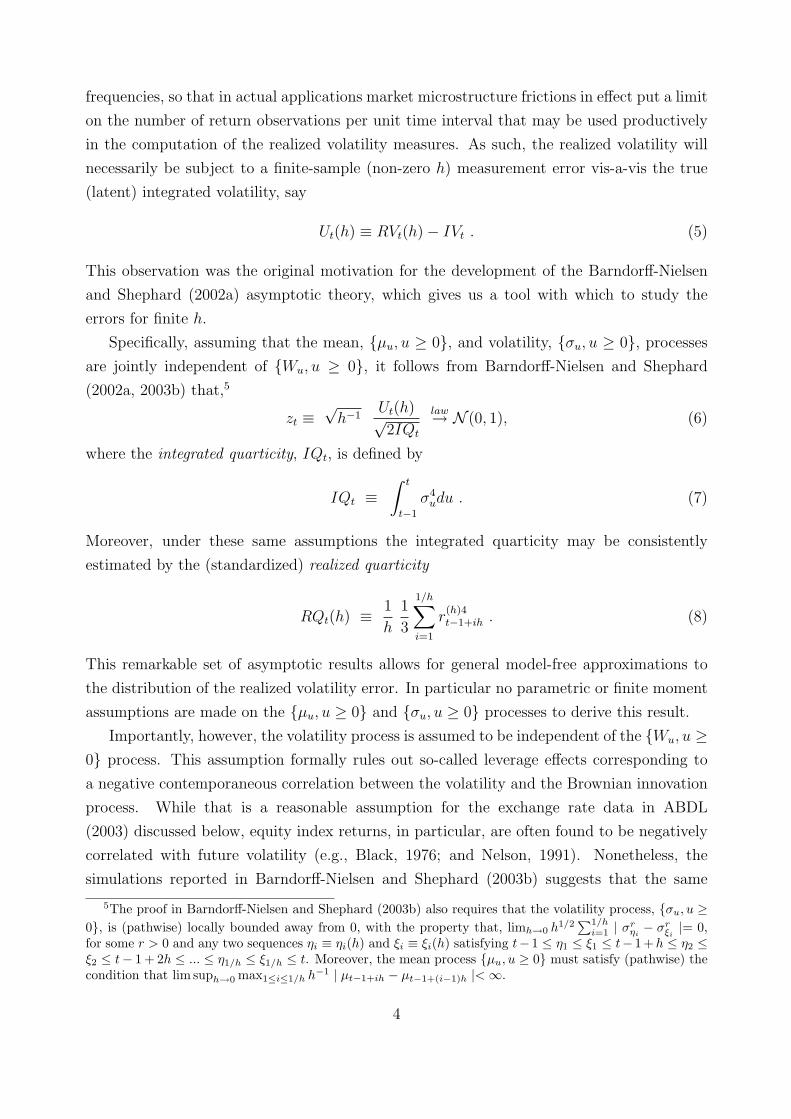
frequencies, so that in actual applications market microstructure frictions in effect put a limit

on the number of return observations per unit time interval that may be used productively

in the computation of the realized volatility measures. As such, the realized volatility will

necessarily be subject to a finite-sample (non-zero h) measurement error vis-a-vis the true

(latent) integrated volatility, say

Ut(h) ≡ RVt(h)− IVt . (5)

This observation was the original motivation for the development of the Barndorff-Nielsen

and Shephard (2002a) asymptotic theory, which gives us a tool with which to study the

errors for finite h.

Specifically, assuming that the mean, {µu, u ≥ 0}, and volatility, {σu, u ≥ 0}, processes

are jointly independent of {Wu, u ≥ 0}, it follows from Barndorff-Nielsen and Shephard

(2002a, 2003b) that,5

zt ≡√

h−1Ut(h)√2IQt

law→ N (0, 1), (6)

where the integrated quarticity, IQt, is defined by

IQt ≡∫ t

t−1

σ4udu . (7)

Moreover, under these same assumptions the integrated quarticity may be consistently

estimated by the (standardized) realized quarticity

RQt(h) ≡ 1

h

1

3

1/h∑i=1

r(h)4t−1+ih . (8)

This remarkable set of asymptotic results allows for general model-free approximations to

the distribution of the realized volatility error. In particular no parametric or finite moment

assumptions are made on the {µu, u ≥ 0} and {σu, u ≥ 0} processes to derive this result.

Importantly, however, the volatility process is assumed to be independent of the {Wu, u ≥0} process. This assumption formally rules out so-called leverage effects corresponding to

a negative contemporaneous correlation between the volatility and the Brownian innovation

process. While that is a reasonable assumption for the exchange rate data in ABDL

(2003) discussed below, equity index returns, in particular, are often found to be negatively

correlated with future volatility (e.g., Black, 1976; and Nelson, 1991). Nonetheless, the

simulations reported in Barndorff-Nielsen and Shephard (2003b) suggests that the same

5The proof in Barndorff-Nielsen and Shephard (2003b) also requires that the volatility process, {σu, u ≥0}, is (pathwise) locally bounded away from 0, with the property that, limh→0 h1/2

∑1/hi=1 | σr

ηi− σr

ξi|= 0,

for some r > 0 and any two sequences ηi ≡ ηi(h) and ξi ≡ ξi(h) satisfying t− 1 ≤ η1 ≤ ξ1 ≤ t− 1+h ≤ η2 ≤ξ2 ≤ t− 1 + 2h ≤ ... ≤ η1/h ≤ ξ1/h ≤ t. Moreover, the mean process {µu, u ≥ 0} must satisfy (pathwise) thecondition that lim suph→0 max1≤i≤1/h h−1 | µt−1+ih − µt−1+(i−1)h |< ∞.

4

(approximate) arguments underlying the Central Limit Theorem in (6) carry over to the case

of a non-zero correlation. We further support this contention through new theoretical results

along with additional simulation based evidence pertaining directly to the measurement error

adjustment procedures developed in the next section.

2.2 Practical Measurement Error Adjustments

The results discussed in the previous section implies that the time t + 1 realized volatility

error is (approximately) serially uncorrelated and orthogonal to any variables (volatility

forecasts) in the time t information set. This justifies the common use of realized volatility

as a convenient simple and unbiased, albeit potentially noisy, benchmark in ex-post volatility

forecast evaluations and model comparisons.

Specifically, consider the Mincer-Zarnowitz style regressions of the realized volatility on

a set of predetermined regressors (volatility forecasts) employed in ABDL (2003) among

others.6 Assuming that the underlying continuous time process satisfies a weak uniform

integrability condition so that the consistency of RQt(h) for IQt also guarantees convergence

in mean (see, e.g., Billingsley, 1994, and Hoffmann-Jørgensen, 1994), it follows directly from

equation (6), that for small values of h,

V ar[IVt] = V ar[RVt(h)] − 2hE[RQt(h)] + o(h). (9)

Thus, any MSE type forecast evaluation criteria based on a comparison of the volatility

forecasts with the ex-post RVt(h) in place of IVt will on average overstate the true variability

of the forecast errors by 2hE[RQt(h)]. In particular, ignoring the o(h) term, it follows

that the (feasible) R2 from the commonly employed Mincer-Zarnowitz regression will under-

estimate the true predictability as measured by the (infeasible) R2 from the regression of the

future (latent) integrated volatility on the same set of predetermined regressors (volatility

forecasts) by the multiplicative factor: V ar[RVt(h)]/{V ar[RVt(h)]− 2hE[RQt(h)]}.7

Meanwhile, the predictive regressions and related loss functions reported in the extant

volatility literature are often formulated in terms of the realized standard deviation,

RVt(h)1/2, or the logarithmic standard deviation, log RVt(h)1/2. To properly gauge the

true predictability in those situations the sample variances of the transformed realized

6Although this is not required for the Barndorff-Nielsen and Shephard (2002a, 2003b) asymptotic theorydiscussed in the previous section, the Mincer-Zarnowitz regression implicitly assumes that the variable ofinterest, i.e., the integrated and realized volatility processes, have finite second order moments. This in turnrequires that the fourth moment of σt is finite. This holds for any affine and log-normal diffusion, and is alsosatisfied for the GARCH diffusions considered in the Monte Carlo experiment discussed in the Appendix.

7As previously noticed by Meddahi (2002), the approximation in (9) also allows for the construction ofmore efficient (in the sense of MSE) model-free integrated volatility estimates, by downweighting the realizedvolatility by the multiplicative factor {V ar[RVt(h)] − 2hE[RQt(h)]}/V ar[RVt(h)] and adding the constant{E[RVt(h)]2hE[RQt(h)]}/V ar[RVt(h)].

5

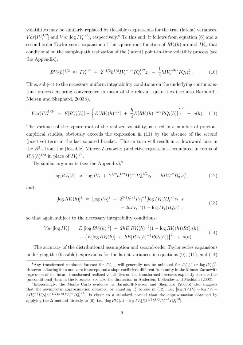
volatilities may be similarly replaced by (feasible) expressions for the true (latent) variances,

V ar[IV1/2t ] and V ar[log IV

1/2t ], respectively.8 To this end, it follows from equation (6) and a

second-order Taylor series expansion of the square-root function of RVt(h) around IVt, that

conditional on the sample-path realization of the (latent) point-in-time volatility process (see

the Appendix),

RVt(h)1/2 ≈ IV1/2t + 2−1/2h1/2IV

−1/2t IQ

1/2t zt −

1

4hIV

−3/2t IQtz

2t . (10)

Thus, subject to the necessary uniform integrability conditions on the underlying continuous-

time process ensuring convergence in mean of the relevant quantities (see also Barndorff-

Nielsen and Shephard, 2003b),

V ar[IV1/2t ] = E[RVt(h)]−

{E[RVt(h)1/2] +

h

4E[RVt(h)−3/2RQt(h)]

}2

+ o(h). (11)

The variance of the square-root of the realized volatility, as used in a number of previous

empirical studies, obviously exceeds the expression in (11) by the absence of the second

(positive) term in the last squared bracket. This in turn will result in a downward bias in

the R2’s from the (feasible) Mincer-Zarnowitz predictive regressions formulated in terms of

RVt(h)1/2 in place of IV1/2t .

By similar arguments (see the Appendix),9

log RVt(h) ≈ log IVt + 21/2h1/2IV −1t IQ

1/2t zt − hIV −2

t IQtz2t , (12)

and,

[log RVt(h)]2 ≈ [log IVt]2 + 23/2h1/2IV −1

t [log IVt]IQ1/2t zt +

− 2hIV −2t (1− log IVt)IQtz

2t ,

(13)

so that again subject to the necessary integrability conditions,

V ar[log IVt] = E[[log RVt(h)]2] − 2hE[RVt(h)−2(1− log RVt(h))RQt(h)]

−{E[log RVt(h)] + hE[RVt(h)−2RQt(h)]

}2+ o(h).

(14)

The accuracy of the distributional assumption and second-order Taylor series expansions

underlying the (feasible) expressions for the latent variances in equations (9), (11), and (14)

8Any transformed unbiased forecast for IVt+1 will generally not be unbiased for IV1/2t+1 or log IV

1/2t+1 .

However, allowing for a non-zero intercept and a slope coefficient different from unity in the Mincer-Zarnowitzregression of the future transformed realized volatilities on the transformed forecasts explicitly corrects this(unconditional) bias in the forecasts; see also the discussion in Andersen, Bollerslev and Meddahi (2003).

9Interestingly, the Monte Carlo evidence in Barndorff-Nielsen and Shephard (2003b) also suggeststhat the asymptotic approximation obtained by equating z2

t to one in (12), i.e., [log RVt(h) − log IVt +hIV −2

t IQt]/[21/2h1/2IV −1t IQ

1/2t ], is closer to a standard normal than the approximation obtained by

applying the ∆-method directly to (6), i.e., [log RVt(h)− log IVt]/[21/2h1/2IV −1t IQ

1/2t ].

6

are underscored by the simulation results for the baseline models reported in Table A1 of

the Appendix.10 It is evident that the simulated medians and ninety-percent confidence

intervals for the asymptotic approximations to V ar[IVt], V ar[IV1/2t ] and V ar[log(IV

1/2t )]

are extremely close to the simulated sampling distributions for the true variances (labelled

h = 1/∞) as long as the frequency of the returns used in the calculation of the realized

volatility and quarticity measures, RVt(h) and RQt(h), respectively, exceeds half-an-hour,

or h ≤ 1/48.

Similar arguments could, of course, be applied for any other twice continuously

differentiable function of integrated volatility in order to obtain an approximate value for

V ar[f(IVt)], in turn allowing for simple model-free approximations to the true (infeasible)

R2’s that would obtain in the hypothetical regressions of f(IVt) on any forecasts by

scaling the (feasible) R2’s from the corresponding regressions based on f(RVt(h)) by the

multiplicative adjustment factor, V ar[f(RVt(h))]/{V ar[f(IVt(h))]}.

2.3 Leverage Effects

The assumptions underlying the distributional results and adjustment procedures discussed

in the previous section formally rule out leverage effects. In order to assess the potential

biases in the various volatility measurements caused by a violation of that assumption, this

section presents analytical results pertaining to the eigenfunction stochastic volatility (ESV)

class of models introduced by Meddahi (2001), explicitly allowing for leverage effects.11

The ESV class of models is very general, encompassing all of the models most commonly

employed in the literature, including the GARCH diffusion model of Nelson (1990), the

log-normal diffusion model popularized by Hull and White (1987) and Wiggins (1987), and

the square-root diffusion model of Heston (1993), along with multi-factor extensions of all

these models.

For expositional purposes, we concentrate on the two-factor ESV model. This remains

the empirically most relevant case. However, all of the analytic results could be extended

to the case of three or more factors without too many technical difficulties, at the cost of

considerable notational complications. The two-factor ESV model is formally defined by the

10The accuracy of (6) and the corresponding CLT for RVt(h)1/2 and log(RVt(h)) based on the ∆-methodhas also previously been investigated by Barndorff-Nielsen and Shephard (2003b).

11The use of eigenfunctions in modelling Markovian time series was pioneered by Chen, Hansen andScheinkman (2000).

7

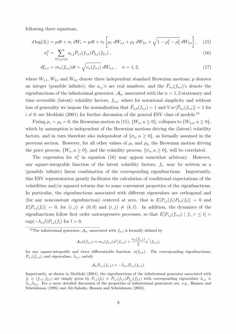
following three equations,

d log(St) = µdt + σt dWt = µdt + σt

[ρ1 dW1,t + ρ2 dW2,t +

√1− ρ2

1 − ρ22 dW3,t

], (15)

σ2t =

∑0≤i,j≤p

ai,jP1,i(f1,t)P2,j(f2,t) , (16)

dfn,t = mn(fn,t)dt +√

vn(fn,t) dWn,t , n = 1, 2, (17)

where W1,t, W2,t and W3,t denote three independent standard Brownian motions; p denotes

an integer (possible infinite); the ai,j’s are real numbers; and the Pn,i(fn,t)’s denote the

eigenfunctions of the infinitesimal generator, An, associated with the n = 1, 2 stationary and

time reversible (latent) volatility factors, fn,t, where for notational simplicity and without

loss of generality we impose the normalization that Pn,0(fn,t) = 1 and V ar[Pn,i(fn,t)] = 1 for

i 6= 0; see Meddahi (2001) for further discussion of the general ESV class of models.12

Fixing ρ1 = ρ2 = 0, the Brownian motion in (15), {Wu, u ≥ 0}, collapses to {W3,u, u ≥ 0},which by assumption is independent of the Brownian motions driving the (latent) volatility

factors, and in turn therefore also independent of {σu, u ≥ 0}, as formally assumed in the

previous section. However, for all other values of ρ1 and ρ2, the Brownian motion driving

the price process, {Wu, u ≥ 0}, and the volatility process, {σu, u ≥ 0}, will be correlated.

The expression for σ2t in equation (16) may appear somewhat arbitrary. However,

any square-integrable function of the latent volatility factors, ft, may be written as a

(possibly infinite) linear combination of the corresponding eigenfunctions. Importantly,

this ESV representation greatly facilitates the calculation of conditional expectations of the

volatilities and/or squared returns due to some convenient properties of the eigenfunctions.

In particular, the eigenfunctions associated with different eigenvalues are orthogonal and

(for any nonconstant eigenfunction) centered at zero, that is E[Pi,j(ft)Pk,l(ft)] = 0 and

E[Pi,j(ft)] = 0, for (i, j) 6= (0, 0) and (i, j) 6= (k, l). In addition, the dynamics of the

eigenfunctions follow first order autoregressive processes, so that E[Pi,j(ft+l) | fτ , τ ≤ t] =

exp(−λi,jl)Pi,j(ft) for l > 0.

12The infinitesimal generator, An, associated with fn,t is formally defined by

Anφ(fn,t) ≡ mn(fn,t)φ′(fn,t) +vn(fn,t)

2φ

′′(fn,t),

for any square-integrable and twice differentiable function, φ(fn,t). The corresponding eigenfunctions,Pn,i(fn,t), and eigenvalues, λn,i, satisfy

AnPn,i(fn,t) = −λn,iPn,i(fn,t).

Importantly, as shown in Meddahi (2001), the eigenfunctions of the infinitesimal generator associated withft ≡ (f1,t, f2,t) are simply given by Pi,j(ft) ≡ P1,i(f1,t)P2,j(f2,t) with corresponding eigenvalues λi,j ≡λ1,iλ2,j . For a more detailed discussion of the properties of infinitesimal generators see, e.g., Hansen andScheinkman (1995) and Aıt-Sahalia, Hansen and Scheinkman (2003).

8

Utilizing these properties of the ESV representation, it is possible to show that for h → 0

(see the Appendix for details),

V ar[Ut(h)] = 2h E [IQt] + o(h), (18)

and

Cov[IVt, Ut(h)] = 2h E[rt] Cov[rt, RVt(h)] + o(h) . (19)

Moreover, the expected integrated quarticity may be estimated by the expected realized

quarticity,

E[RQt(h)] = E[IQt] + o(1) . (20)

This latter results would, of course, be implied by the aforementioned consistency of RQt(h)

for IQt under appropriate uniform integrability conditions. However, the corresponding

proof of consistency in Barndorff-Nielsen and Shephard (2003a) again rules out leverage

effects.13 Now, combining the results in (18), (19), and (20), it follows readily that

V ar[IVt] = V ar[RVt(h)] − V ar[Ut(h)] − 2Cov[Ut(h), IVt]

= V ar[RVt(h)] − 2h E[RQt(h)] − 4h E[rt] Cov[rt, RVt(h)] + o(h).

(21)

Hence, relative to (9), the leverage effect introduces the additional 4hE[rt]Cov[rt, RVt(h)]

term in the (feasible) asymptotic approximation to V ar[IVt].

In actual empirical applications 2E[rt] and Cov[rt, RVt(h)] will both generally be orders of

magnitude smaller than E[RQt(h)] so that, invariably, the magnitude of the new adjustment

term will be very small (negligible) relative to the 2hE[RQt(h)] term. To illustrate, consider

the five-minute high-frequency S&P500 and U.S. T-Bond futures returns spanning the period

from January 1990 through December 2002.14 The relative importance of the leverage

adjustment term, as measured by the daily 2E[rt]Cov[rt, RVt(h)]/E[RQt(h)] ratios, equal

−7.85 × 10−5 and −6.94 × 10−4 for each of the two markets. Also, for the DM/$, Yen/$,

and Yen/DM half-hour returns underlying the empirical results in ABDL (2003) discussed

below, these same daily ratios for the full December 1986 through June 1999 sample period

equal 1.01 × 10−4, −7.87 × 10−5, and 3.54 × 10−4, respectively. Clearly an inconsequential

addition to the approximation for V ar[IVt] in (9).

These empirical observations are further corroborated by the Monte Carlo simulation

results for the leverage models with constant as well as time-varying drifts reported in Tables

A2 and A3. The medians in the asymptotic approximations to V ar[IVt], V ar[IV1/2t ] and

13Related general results are available in Lepingle (1976) and the thesis by Becker (1998) in an abstractsetting; see also Barndorff-Nielsen, Graversen and Shephard (2003).

14The data has previously been analyzed in Andersen, Bollerslev, Diebold and Vega (2003) from a verydifferent perspective. We refer the reader to that study for a more detailed description of the data sourceand return construction.

9

V ar[log(IV1/2t )] in equations (9), (11), and (14), respectively, derived under the assumption

of no leverage are all right-on the true medians (labelled h = 1/∞). Moreover, as

long as the frequency of the returns used in the calculation of the realized volatility and

quarticity measures exceeds half-an-hour, or h ≤ 1/48, the simulated distributions for the

leverage models are indistinguishable from the corresponding distributions for the same

models without leverage reported in Table A1. In short, the realized volatility measurement

error adjustment procedures developed in the preceding section remain highly accurate in

empirically realistic situations allowing for both leverage and time-varying drift. We next

turn to a re-interpretation of the empirical evidence related to the Mincer-Zarnowitz volatility

regressions reported in ABDL (2003) based on an application of these procedures.

3 ABDL (2003) Revisited

The forecast comparisons in ABDL (2003) are based on daily realized volatilities constructed

from high-frequency half-hourly, or h=1/48, spot exchange rates for the U.S. dollar, the

Deutschemark and the Japanese yen spanning twelve-and-a-half years.15 Separate forecast

evaluation regressions are reported for the “in-sample” period comprised of the 2,449

“regular” trading days from December 1, 1986 through December 1, 1996, and the shorter

“out-of-sample” forecast period consisting of the 596 days from December 2, 1996 through

June 30, 1999. Separate results are also reported for one-day-ahead and ten-days-ahead

forecasts. However, for all series and both sample periods and forecast horizons, a simple

AR(5) model estimated directly from the realized volatilities generally performs as well or

better than any of the many alternative models considered, including several GARCH type

models estimated directly to the high-frequency data (both with and without corrections

for the pronounced intradaily seasonal pattern in volatility). The representative R2’s

for the DM/$, Yen/$, and Yen/DM forecast regressions for RVt+1(1/48), RVt+1(1/48)1/2,

log RVt+1(1/48)1/2, RVt+10,10(1/48), RVt+10,10(1/48)1/2, and log RVt+10,10(1/48)1/2, where

RVt+10,10(1/48) ≡ RVt+1(1/48) + RVt+2(1/48) + ... + RVt+10(1/48), as reported in ABDL

(2003) and the accompanying appendix, are given in square brackets in Table 1.16

By failing to account for the measurement errors in the future realized volatilities, these

R2’s understate the true degree of predictability in the (latent) integrated volatilities. This

problem is rectified by the main entries in Table 1, which report the adjusted R2’s obtained

15The high-frequency data were generously provided by Olsen & Associates in Zurich, Switzerland; seeDacorogna, Gencay, Muller, Olsen and Pictet (2001) for further discussion of the data capture, filtering, andreturn construction.

16The out-of-sample period contains a “once-in-a-generation” move in the Japanese Yen on October 8,1998. Somewhat higher R2’s, but qualitatively similar results, were obtained by excluding this and theneighboring two days; see ABDL (2003) and the accompanying appendix for further discussion and sensitivityanalysis along these lines.

10

by applying the (feasible) asymptotic approximations in equations (9), (11), and (14), along

with the relevant multiplicative adjustment factors.17 The results are quite striking. For

some of the forecasts horizons and rates, the “true” R2’s exceed the standard predictive

R2’s, as reported in ABDL (2003), by up to forty percent. For instance, the in-sample,

one-day-ahead R2 for the DM/$ series given in the very first entry in the table equals 0.219,

whereas the true (albeit estimated) R2 is substantially higher at 0.314. As such, the results

clearly highlight the importance of appropriately adjusting for measurement error when

assessing the quality of volatility forecasts in practical empirical applications.

Table 1

ABDL (2003) Adjusted Predictive R2’s

IV IV 1/2 log IV 1/2

In-Sample, One-Day-AheadDM/$ 0.314 [0.219] 0.399 [0.351] 0.482 [0.431]Yen/$ 0.315 [0.229] 0.412 [0.374] 0.476 [0.433]Yen/DM 0.450 [0.361] 0.559 [0.499] 0.630 [0.567]Out-of-Sample, One-Day-AheadDM/$ 0.200 [0.158] 0.296 [0.246] 0.350 [0.285]Yen/$ 0.230 [0.197] 0.366 [0.338] 0.419 [0.373]Yen/DM 0.215 [0.189] 0.378 [0.344] 0.483 [0.424]In-Sample, Ten-Days-AheadDM/$ 0.411 [0.374] 0.463 [0.436] 0.499 [0.473]Yen/$ 0.386 [0.355] 0.414 [0.396] 0.424 [0.407]Yen/DM 0.536 [0.513] 0.606 [0.589] 0.653 [0.637]Out-of-Sample, Ten-Days-AheadDM/$ 0.182 [0.168] 0.209 [0.195] 0.228 [0.213]Yen/$ 0.197 [0.187] 0.287 [0.279] 0.347 [0.336]Yen/DM 0.186 [0.178] 0.301 [0.293] 0.401 [0.390]

Note: The table reports the adjusted predictive R2’s from the Mincer-Zarnowitz regressions of therealized volatilities on the AR(5) volatility forecasts in ABDL (2003), along with the correspondingunadjusted R2’s (in square brackets). The realized volatility measures are constructed from high-frequency half-hour returns. The “in-sample” period covers December 1, 1986 through December1, 1996, while the “out-sample” period spans December 2, 1996 through June 30, 1999.

Interestingly, the numerical values for the adjusted R2’s for the DM-dollar series in Table 1

are quite close to the exact theoretical R2’s implied by the specific two-factor affine diffusion

discussed in Andersen, Bollerslev and Meddahi (2003). This is especially noteworthy in

so far the parameter values for this model are based on the identical DM-dollar sample

17The adjustments are constructed separately for each series and for the in-sample and out-of-sampleperiods using the corresponding realized volatility and quarticity series.

11

underlying the results reported on in Table 1. This suggests that the simple AR(5) models

for the realized volatilities estimated in ABDL (2003) - when adjusted for the measurement

error problem - capture a degree of predictability that is consistent with that implied by

a conventional two-factor affine model. This type of benchmarking of the true predictive

power of such reduced-form forecast procedures relative to that of a specific continuous-time

volatility model would, of course, be impossible without the type of measurement error

correction developed here.

4 Concluding Remarks

Building on the recent theoretical results of Barndorff-Nielsen and Shephard (2002a, 2003a),

this note develops a set of simple and practically feasible expressions for calculating true

measures of return volatility predictability relative to that of the corresponding underlying

(latent) integrated volatility. The procedures are general and could be applied in the

evaluation of any volatility forecasts. The analytical results for the eigenfunction stochastic

volatility class of models and accompanying simulation based evidence confirm that the

procedures work equally well in situations with pronounced leverage effects. On specifically

applying the procedures to the ex-post forecast evaluation regressions reported in ABDL

(2003), we document sizeable downward biases in terms of the previously reported predictive

powers. More generally, the practical techniques developed here hold the promise for further

development of new and improved easy-to-implement volatility forecasting procedures guided

by proper benchmark comparisons. The techniques should also prove useful in more

effectively calibrating the type of continuous-time models routinely employed in modern

asset pricing theories.

12

Appendix 1: Monte Carlo Simulations

In order to assess the accuracy of the distributional assumptions and second-order Taylor series expansionsunderlying the asymptotic approximations in (9), (11), and (14) in empirically relevant specifications andsample sizes compatible with those of ABDL (2003), Tables A1-A3 report the simulated medians and ninety-percent confidence intervals (in square brackets) across 1,000 replications, each consisting of 2,500 “days.”We report the results for a total of nine different continuous-time models along with 1/h = 288, 96, 48, and1, corresponding to the use of “5-minute,” “15-minute,” “half-hourly,” and “daily” returns.

The first three models reported in Table A1 fix the mean returns at zero, and assume that the volatilityand the Brownian motion driving the price process are independent, i.e., no leverage effects. In the notationof equation (15), µ = ρ1 = ρ2 = 0,

d log(St) = σtdW3,t.

The numbers in the first panel refer to the GARCH(1,1) diffusion analyzed in Andersen and Bollerslev(1998),

dσ2t = 0.035(0.636− σ2

t )dt + 0.144 σ2t dW1,t .

The second panel gives the results for the two-factor affine diffusion estimated by Bollerslev and Zhou (2002),σ2

t = σ21,t + σ2

2,t, where

dσ21,t = 0.5708(0.3257− σ2

1,t)dt + 0.2286 σ1,tdW1,t ,

dσ22,t = 0.0757(0.1786− σ2

2,t)dt + 0.1096 σ2,tdW2,t .

These parameter values were obtained from estimation based on the identical DM-dollar sample used inABDL (2003). The third set of numbers refer to the log-normal diffusion reported in Andersen, Benzoni andLund (2002) with volatility dynamics governed by

d log(σ2t ) = − 0.0136[0.8382 + log(σ2

t )]dt + 0.1148 dW1,t .

All of the models in Table A1 satisfy the Barndorff-Nielsen and Shephard (2002a, 2003b) regularity conditionsdiscussed in Sections 2.1 and 2.2.

The results reported in Table A2 are based on the same three volatility specifications, but incorporatea positive drift and strong leverage effects. For the one-factor GARCH and log-normal diffusions,

d log(St) = 0.0314 dt + σt[−0.576 dW1,t +√

1− 0.5762dW3,t] ,

where the values for the drift and leverage parameters are taken from Andersen, Benzoni and Lund (2002).For the two-factor affine model the instantaneous return dynamic is governed by,

d log(St) = 0.0314 dt + σt[0.9 dW1,t − 0.4 dW2,t +√

1− 0.92 − 0.42dW3,t] ,

with the two leverage parameters adapted from the estimates reported in Chernov, Gallant, Ghysels andTauchen (2003).

In addition to the contemporaneous correlation between the return and volatility for the leverage modelsin Table A2, the last set of models in Table A3 also include a volatility feedback, or ARCH-in-mean, effectin the drift component. Specifically, for the two one-factor models,

d log(St) = (0.0314 + 0.3σ2t ) dt + σt[−0.576 dW1,t +

√1− 0.5762dW3,t] ,

while for the two-factor model,

d log(St) = (0.0314 + 0.3σ2t ) dt + σt[0.9 dW1,t − 0.4 dW2,t +

√1− 0.92 − 0.42dW3,t] .

The value of the slope coefficient in the drift is taken from Chernov (2003).

13

Table A1: Asymptotic Variance ApproximationsBaseline Volatility Models

h V ar[IVt] V ar[IV1/2t ] V ar[log(IV

1/2t )]

GARCH(1,1) Diffusion1/∞ 0.170 0.0647 0.138

[0.117, 0.265] [0.0518, 0.0853] [0.112, 0.168]1/288 0.170 0.0647 0.138

[0.116, 0.266] [0.0517, 0.0854] [0.112, 0.168]1/96 0.171 0.0648 0.138

[0.116, 0.266] [0.0520, 0.0859] [0.112, 0.168]1/48 0.170 0.0650 0.139

[0.115, 0.268] [0.0520, 0.0861] [0.112, 0.169]1 0.167 0.208 1.19

[0.0923, 0.313] [0.175, 0.248] [1.08, 1.30]Two-Factor Affine1/∞ 0.0259 0.0126 0.0261

[0.0222, 0.0316] [0.0111, 0.0145] [0.0235, 0.0290]1/288 0.0260 0.0126 0.0261

[0.0222, 0.0316] [0.0111, 0.0145] [0.0234, 0.0291]1/96 0.0260 0.0126 0.0263

[0.0221, 0.0315] [0.0111, 0.0146] [0.0235, 0.0294]1/48 0.0259 0.0127 0.0267

[0.0219, 0.0315] [0.0112, 0.0148] [0.0238, 0.0302]1 0.0245 0.136 1.07

[0.00617, 0.0462] [0.125, 0.149] [0.973, 1.16]Log-Normal Diffusion1/∞ 0.145 0.0544 0.109

[0.0640, 0.333] [0.0328, 0.0946] [0.0764, 0.163]1/288 0.144 0.0543 0.109

[0.0643, 0.338] [0.0330, 0.0943] [0.0762, 0.163]1/96 0.145 0.0546 0.109

[0.0642, 0.337] [0.0330, 0.0952] [0.0766, 0.164]1/48 0.144 0.0547 0.109

[0.0635, 0.341] [0.0331, 0.0953] [0.0769, 0.165]1 0.145 0.177 1.15

[0.0529, 0.390] [0.127, 0.252] [1.05, 1.27]

Note: The table reports the simulated medians and ninety-percent confidence intervals (in squarebrackets) for the asymptotic approximations in equations (9), (11), and (14) across 1,000 replications, eachconsisting of 2,500 ”days.”

14

Table A2: Asymptotic Variance ApproximationsVolatility Models with Leverage and Constant Drift


1/2t )]

GARCH(1,1) Diffusion1/∞ 0.170 0.0647 0.138

[0.117, 0.265] [0.0518, 0.0853] [0.112, 0.168]1/288 0.170 0.0647 0.138

[0.116, 0.262] [0.0518, 0.0849] [0.112, 0.168]1/96 0.170 0.0647 0.138

[0.116, 0.265] [0.0520, 0.0852] [0.112, 0.168]1/48 0.170 0.0650 0.138

[0.115, 0.268] [0.0520, 0.0853] [0.113, 0.168]1 0.165 0.205 1.16


[0.0222, 0.0316] [0.0111, 0.0145] [0.0235, 0.0290]1/288 0.0260 0.0126 0.0261

[0.0221, 0.0317] [0.0111, 0.0145] [0.0234, 0.0292]1/96 0.0261 0.0127 0.0263

[0.0222, 0.0321] [0.0112, 0.0145] [0.0236, 0.0294]1/48 0.0262 0.0129 0.0267

[0.0221, 0.0323] [0.0112, 0.0150] [0.0239, 0.0301]1 0.0370 0.139 1.07


[0.0640, 0.333] [0.0328, 0.0946] [0.0764, 0.163]1/288 0.144 0.0545 0.109

[0.0640, 0.336] [0.0329, 0.0941] [0.0763, 0.162]1/96 0.145 0.0545 0.109

[0.0637, 0.337] [0.0331, 0.0952] [0.0763, 0.163]1/48 0.146 0.0547 0.110

[0.0635, 0.340] [0.0335, 0.0943] [0.0766, 0.162]1 0.145 0.177 1.15

[0.0515, 0.375] [0.127, 0.251] [1.04, 1.27]

Note: See Table A1.

15

Table A3: Asymptotic Variance ApproximationsVolatility Models with Leverage and Time-Varying Drift


1/2t )]

GARCH(1,1) Diffusion1/∞ 0.170 0.0647 0.138

[0.117, 0.265] [0.0518, 0.0853] [0.112, 0.168]1/288 0.170 0.0648 0.138

[0.116, 0.262] [0.0518, 0.0850] [0.112, 0.168]1/96 0.171 0.0647 0.138

[0.116, 0.266] [0.0521, 0.0853] [0.112, 0.168]1/48 0.171 0.0652 0.138

[0.116, 0.270] [0.0521, 0.0855] [0.113, 0.168]1 0.196 0.225 1.17


[0.0222, 0.0316] [0.0111, 0.0145] [0.0235, 0.0290]1/288 0.0261 0.0126 0.0262

[0.0222, 0.0318] [0.0111, 0.0146] [0.0235, 0.0292]1/96 0.0264 0.0128 0.0265

[0.0225, 0.0324] [0.0113, 0.0147] [0.0238, 0.0296]1/48 0.0268 0.0131 0.0272

[0.0226, 0.0329] [0.0115, 0.0152] [0.0243, 0.0306]1 0.0661 0.163 1.09


[0.0640, 0.333] [0.0328, 0.0946] [0.0764, 0.163]1/288 0.145 0.0545 0.109

[0.0641, 0.336] [0.0329, 0.0942] [0.0764, 0.163]1/96 0.145 0.0546 0.109

[0.0639, 0.337] [0.0332, 0.0954] [0.0764, 0.163]1/48 0.146 0.0548 0.110

[0.0636, 0.342] [0.0336, 0.0948] [0.0768, 0.163]1 0.164 0.192 1.15

[0.0608, 0.543] [0.136, 0.281] [1.04, 1.27]

Note: See Table A1.

16

Appendix 2: Technical Proofs

Proof of equations (10), (11), (12), (13), and (14). Let f(·) be a twice-differentiable function. By (6)and a second order Taylor approximation of f(·) at the point RVt(h) around IVt, it follows that

f(RVt(h)) ≈ f(IVt) + f ′(IVt)√

2hIQt zt +12f ′′(IVt)2hIQt z2

t . (A.1)

Consequently,

E[f(RVt(h))] = E[f(IVt)] + E[f ′(IVt)√

2hIQt zt] +12E[f ′′(IVt)2hIQt z2

t ] + o(h)

= E[f(IVt)] + E[f ′(IVt)√

2hIQtE[zt | σu, t− 1 ≤ u ≤ t]]

+12E[f ′′(IVt)2hIQtE[z2

t | σu, t− 1 ≤ u ≤ t]] + o(h)

= E[f(IVt)] +12E[f ′′(IVt)2hIQt] + o(h),

so that,

E[f(RVt(h))] = E[f(IVt)] +12E[f ′′(RVt(h))2hRQt(h)] + o(h) (A.2)

provided E[f ′′(RVt(h))RQt(h)]−E[f ′′(IVt)IQt] = o(1). Equations (10), (12), and (13) follows by applying(A.1) to the functions f1(x) = x1/2, f2(x) = log(x), and f3(x) = log(x)2, where f ′1(x) = 2−1x−1/2,f ′′1 (x) = −2−2x−3/2, f ′2(x) = x−1, f ′′2 (x) = −x−2, f ′3(x) = 2x−1 log(x), and f ′′3 (x) = 2x−2(1 − log(x)). Byapplying (A.2) to the function f1(·), one gets (11). Similarly, by applying (A.2) to the functions f2(·) andf3(·), one gets (14).�

Proof of equation (18). By definition,

Ut(h) =1/h∑i=1

u(h)t−1+ih where u

(h)t−1+ih ≡ r

(h)2t−1+ih −

∫ t−1+ih

t−1+(i−1)h

σ2udu.

By similar arguments to Meddahi (2002), Proposition 4.2, it follows that the u(h)t−1+ih’s are uncorrelated, so

that

V ar[Ut(h)] = V ar

1/h∑i=1

u(h)t−1+ih

=V ar[u(h)

t−1+ih]h

.

Hence, by Ito’s Lemma,u

(h)t−1+ih = µ2h2 + 2µhε

(h)t−1+ih + 2Z

(h)t−1+ih

where

ε(h)t−1+ih =

∫ t−1+ih

t−1+(i−1)h

σudWu, Z(h)t−1+ih =

∫ t−1+ih

t−1+(i−1)h

(∫ u

t−1+(i−1)h

σsdWs

)σudWu.

Therefore,V ar[u(h)

h ] = 4µ2h2V ar[ε(h)h ] + 4V ar[Z(h)

h ] + 8µhCov(ε(h)h , Z

(h)h )

In the sequel, we will show that for h → 0,

V ar[ε(h)h ] = o(1), (A.3)

V ar[Z(h)h ] =

h2

2

∑0≤i,j≤p

a2i,j + o(h2), (A.4)

Cov(ε(h)h , Z

(h)h ) = o(h), (A.5)

which in turn implies thatV ar[u(h)

h ] = h2 2∑

0≤i,j≤p

a2i,j + o(h2) ,

17

and thusV ar[h−1/2Ut(h)] = 2

∑0≤i,j≤p

a2i,j + o(1).

By formulas (4.2) and (4.5) in Andersen, Bollerslev and Meddahi (2003), E[σ4t ] =

∑0≤i,j≤p

a2i,j , which combined

with (7), achieves the proof of (18).Proof of (A.3): By definition of ε

(h)h , ε

(h)2h =

∫ h

0σ2

udu and E[ε(h)h ] = 0. Hence

V ar[ε(h)h ] = E[ε(h)2

h ] =∫ h

0

E[σ2u]du = a0,0h, (A.6)

given that E[Pi,j(fu)] = 0 when i 6= 0 or j 6= 0, which implies (A.3).Proof of (A.4): Note that

V ar[Z(h)h ] = E

[∫ h

0

(∫ u

0

σsdWs

)2

σ2udu

]

= E

[∫ h

0

(∫ u

0

σ2sds

)σ2

udu

]+ 2E

[∫ h

0

(∫ u

0

(∫ s

0

σwdWw

)σsdWs

)σ2

udu

]

= E

[∫ h

0

(∫ u

0

σ2sds

)σ2

udu

]+ 2E

[∫ h

0

Z(u)u σ2

udu

]

=∫ h

0

(∫ u

0

E[σ2sσ2

u]ds

)du + 2

∑0≤i,j≤p

ai,j

∫ h

0

E[Z(u)u Pi,j(fu)]du.

Denoting λi,j = λ1,iλ2,j , it follows from (4.2) and (4.8) in Andersen, Bollerslev and Meddahi (2003) that

∀s, u, s ≤ u : E[σ2sσ2

u] =∑

0≤i,j≤p

a2i,j exp(−λi,j(u− s)),

and therefore∫ h

0

(∫ u

0

E[σ2sσ2

u]ds

)du =

∑0≤i,j≤p

a2i,j

1λ2

i,j

[exp(−λi,jh)− 1 + λi,jh] =h2

2

∑0≤i,j≤p

a2i,j + o(h2).

Thus, in order to prove (A.4), it suffice to show that∫ h

0

E[Z(u)u Pi,j(fu)]du = o(h2). (A.7)

Applying (A2) in Meddahi (2002) to the factors fn,t, n = 1, 2, it follows that

Pn,i(fn,u) = exp(−λn,i(u−s))Pn,i(fn,s)+exp(−λn,i(u−s))∫ u

s

exp(λn,i(w−s))√

vn(fn,w)P ′n,i(fn,w) dWn,w,

Pi,j(fu) = P1,i(f1,u)P2,j(f2,u) = exp(−λi,j(u− s))×{Pi,j(fs) + P1,i(f1,s)

∫ u

s

exp(λ2,j(w − s))√

v2(f2,w)P ′2,j(f2,w) dW2,w

+P2,j(f2,s)∫ u

s

exp(λ1,i(w − s))√

v1(f1,w)P ′1,i(f1,w) dW1,w

+∫ u

s


v1(f1,w)P ′1,i(f1,w) dW1,w

∫ u

s


v2(f2,w)P ′2,j(f2,w) dW2,w

}.

However, by Ito’s Lemma,∫ u

s


v1(f1,w)P ′1,i(f1,w) dW1,w

∫ u

s


v2(f2,w)P ′2,j(f2,w) dW2,w

=∫ u

s


v1(f1,w)P ′1,i(f1,w)

[∫ w

s

exp(λ2,j(z − s))√

v2(f2,w)P ′2,j(f2,z) dW2,z

]dW1,w

18

+∫ u

s


v2(f2,w)P ′2,j(f2,w)

[∫ w

s

exp(λ1,i(z − s))√

v1(f1,w)P ′1,i(f1,z) dW1,z

]dW2,w.

Thus,

Pi,j(fu) = exp(−λi,j(u− s))×{Pi,j(fs) + P1,i(f1,s)

∫ u

s


v2(f2,w)P ′2,j(f2,w) dW2,w

+P2,j(f2,s)∫ u

s


v1(f1,w)P ′1,i(f1,w) dW1,w

+∫ u

s


v1(f1,w)P ′1,i(f1,w)

[∫ w

s

exp(λ2,j(z − s))√

v2(f2,w)P ′2,j(f2,z) dW2,z

]dW1,w

+∫ u

s


v2(f2,w)P ′2,j(f2,w)

[∫ w

s

exp(λ1,i(z − s))√

v1(f1,w)P ′1,i(f1,z) dW1,z

]dW2,w

}.

(A.8)Consequently,

E[Z(u)u Pi,j(fu)] = E

[∫ u

0

(∫ s

0

σwdWw

)σs exp(−λi,j(u− s))P1,i(f1,s)

√v2(f2,s)P ′

2,j(f2,s)ρ2ds

]+ E

[∫ u

0

(∫ s

0

σwdWw

)σs exp(−λi,j(u− s))P2,j(f2,s)

√v1(f1,s)P ′

1,i(f1,s)ρ1ds

],

i.e., the first, fourth and fifth terms on the right-hand side of (A.8) do not contribute to E[Z(u)u Pi,j(fu)].

Now define the reals ni,j , ei,j,k,l, mi,j , and di,j,k,l by the expansions in mean-square:

σsP1,i(f1,s)√

v2(f2,s)P ′2,j(f2,s) =

∑0≤k,l≤ni,j

ei,j,k,lPk,l(fs),

σsP2,j(f2,s)√

v1(f1,s)P ′1,i(f1,s) =

∑0≤k,l≤mi,j

di,j,k,lPk,l(fs).

Then,

E[Z(u)u Pi,j(fu)] = ρ2

∑0≤k,l≤ni,j

ei,j,k,lE

[∫ u

0

(∫ s

0

σwdWw

)exp(−λi,j(u− s))Pk,l(fs)ds

]

+ ρ1

∑0≤k,l≤mi,j

di,j,k,lE

[∫ u

0

(∫ s

0

σwdWw

)exp(−λi,j(u− s))Pk,l(fs)ds

]

= ρ2

∑0≤k,l≤ni,j

ei,j,k,l

∫ u

0

(∫ s

0

E[Pk,l(fs)σwdWw])

exp(−λi,j(u− s))ds

+ ρ1

∑0≤k,l≤mi,j

di,j,k,l

∫ u

0

(∫ s

0

E[Pk,l(fs)σwdWw])

exp(−λi,j(u− s))ds.

Moreover,

E[Pk,l(fs)σwdWw]

= exp(−λk,l(s− w))E[ρ1P2,l(f2,w)

√v1(f1,w)P ′

1,k(f1,w) + ρ2P1,i(f1,w)√

v2(f2,w)P ′2,l(f2,w)

]dw

= exp(−λk,l(s− w))(ρ1dk,l,0,0 + ρ2ek,l,0,0)dw. (A.9)

Hence,

19

E[Z(u)u Pi,j(fu)]

= ρ2

∑0≤k,l≤ni,j

ei,j,k,l(ρ1dk,l,0,0 + ρ2ek,l,0,0)∫ u

0

(∫ s

0

exp(−λk,l(s− w))dw])


+ ρ1

∑0≤k,l≤mi,j

di,j,k,l(ρ1dk,l,0,0 + ρ2ek,l,0,0)∫ u

0

(∫ s

0

exp(−λk,l(s− w))dw])


= ρ2

∑0≤k,l≤ni,j

ei,j,k,l(ρ1dk,l,0,0 + ρ2ek,l,0,0)(

1− exp(−λi,ju)λi,jλk,l

− exp(−λk,lu)− exp(−λi,ju)(λi,j − λk,l)λk,l

)

+ ρ1

∑0≤k,l≤mi,j

di,j,k,l(ρ1dk,l,0,0 + ρ2ek,l,0,0)(



). (A.10)

Therefore,∫ h

0

E[Z(u)u Pi,j(fu)]du

= ρ2

∑0≤k,l≤ni,j

ei,j,k,l(ρ1dk,l,0,0 + ρ2ek,l,0,0)∫ h

0

(1− exp(−λi,ju)

λi,jλk,l− exp(−λk,lu)− exp(−λi,ju)

(λi,j − λk,l)λk,l

)du

+ ρ1

∑0≤k,l≤mi,j

di,j,k,l(ρ1dk,l,0,0 + ρ2ek,l,0,0)∫ h

0




)du.

But∫ h

0




)du

=1

λk,l

[h

λi,j− 1− exp(−λi,jh)

λ2i,j

− 1− exp(−λk,lh)(λi,j − λk,l)λk,l

+1− exp(−λi,jh)(λi,j − λk,l)λi,j

]=

16h3 + o(h3),

which implies (A.7) and therefore (A.4).Proof of (A.5): Since E[ε(h)

h ] = 0, Cov(ε(h)h , Z

(h)h ) = E[ε(h)

h Z(h)h ]. By Ito’s Lemma,

ε(h)h Z

(h)h =

∫ h

0

Z(u)u dε(u)

u +∫ h

0

ε(u)u dZ(h)

u +∫ h

0

d[Z, ε]u,

where [Z, ε]u denotes the quadratic covariation of Z(u)u and ε

(u)u over the interval [0, u], i.e.,

[Z, ε]u =∫ u

0

(∫ s

0

σwdWw

)σ2

sds =∫ u

0

ε(s)s σ2

sds.

Note that E[∫ h

0Z

(u)u dε

(u)u ] = 0 and E[

∫ h

0ε(u)u dZ

(u)u ] = 0. Hence,

E[ε(h)h Z

(h)h ] = E

[∫ h

0

ε(u)u σ2

udu

]=

∑0≤i,j≤p

ai,j

∫ h

0

E[ε(u)u Pi,j(fu)]du =

∑0≤i,j≤p

ai,j

∫ h

0

∫ u

0

E[σsdWsPi,j(fu)]du.

(A.11)Lastly, by (A.9),

E[ε(h)h Z

(h)h ] =

∑0≤i,j≤p

ai,j

∫ h

0

∫ u

0

exp(−λi,j(u− s)) (ρ2ei,j,00 + ρ1di,j,0,0) dsdu

=∑

0≤i,j≤p

ai,j (ρ2ei,j,00 + ρ1di,j,0,0)1

λ2i,j

[exp(−λi,jh)− 1 + λi,jh)]

=h2

2

∑0≤i,j≤p

ai,j (ρ2ei,j,00 + ρ1di,j,0,0) + o(h2),

20

which implies (A.5), and achieves the proof of (18).

Proof of equation (20). By definition,

E[RQt(h)] =13h

E

1/h∑i=1

r(h)4t−1+ih

=1

3h2E[r(h)4

h ].

Thus, it suffice to show thatE[r(h)4

h ] = 3h2∑

0≤i,j≤p

a2i,j + o(h2). (A.12)

Note that by (A.6), r(h)h = µh + ε

(h)h and E[ε(h)2

h ] = a0,0h. Hence,

E[r(h)4h ] = V ar[r(h)2

h ] + E[r(h)2h ]2 = V ar[r(h)2

h ] + (µ2h2 + ha0,0)2 = V ar[r(h)2h ] + a2

0,0h2 + o(h2). (A.13)

In addition, by using Ito’s Lemma for k = 1, ..., 1/h,

r(h)2kh = µ2h2 + ε

(h)2kh + 2µhε

(h)kh = µ2h2 + iv

(h)kh + 2Z

(h)kh + 2µhε

(h)kh where iv

(h)kh =

∫ kh

(k−1)h

σ2udu.

Therefore,V ar[r(h)2

h ] = V ar[iv(h)h ] + 4V ar[Z(h)

h ] + 4µ2h2V ar[ε(h)h ]

+4Cov(iv(h)h , Z

(h)h ) + 4µhCov(iv(h)

h , ε(h)h ) + 8µhCov(Z(h)

h , ε(h)h ). (A.14)

In the sequel, we will show that

V ar[iv(h)h ] = h2

∑0≤i,j≤p,(i,j) 6=(0,0)

a2i,j + o(h2), (A.15)

Cov(iv(h)h , Z

(h)h ) = o(h2), (A.16)

Cov(iv(h)h , ε

(h)h ) = o(h). (A.17)

Combining (A.13) and (A.14), along with (A.4), (A.5), (A.15), (A.16), and (A.17), achieves the proof of(A.12).Proof of (A.15): By (4.5) in Andersen, Bollerslev and Meddahi (2003) it follows that

V ar[iv(h)h ] = 2

∑0≤i,j≤p, (i,j) 6=(0,0)

a2i,j

λ2i,j

[exp(−λi,jh) + λi,jh− 1] = h2∑

0≤i,j≤p, (i,j) 6=(0,0)

a2i,j + o(h2).

Proof of (A.16): The quadratic covariation of iv(h)h and Z

(h)h is zero. Hence, by Ito’s Lemma

iv(h)h Z

(h)h =

∫ h

0

Z(u)u div(u)

u +∫ h

0

iv(u)u dZ(u)

u =∫ h

0

Z(u)u σ2

udu +∫ h

0

iv(u)u

(∫ u

0

σsdWs

)σudWu,

which implies (A.16) since

Cov(iv(h)h , Z

(h)h ) = E(iv(h)

h Z(h)h ) =

∫ h

0

E[Z(u)u σ2

u]du =∑

0≤i,j≤p

ai,j

∫ h

0

E[Z(u)u Pi,j(u)]du = o(h2),

where the last equality holds by (A.7).Proof of (A.17): By similar arguments to the ones above, the quadratic covariation between iv

(h)h and ε

(h)h

equals zero. Hence, using Ito’s Lemma

E[iv

(h)h ε

(h)h

]= E

[∫ h

0

ε(u)u div(u)

u +∫ h

0

iv(u)u dε(u)

u

]= E

[∫ h

0

ε(u)u σ2

udu

]= E[ε(h)

h Z(h)h ],

21

where the last equality holds by the first equality in (A.11), so that (A.5) implies (A.17).

Proof of equation (19). Note that ε(1)1 = r1 − µ, where µ = E[rt] and ε

(1)1 =

∑1/hk=1 ε

(h)kh . Thus,

Cov(Ut(h), IVt) = Cov(U1(h), IV1) = Cov(1/h∑k=1

u(h)kh , IV1) = Cov

1/h∑k=1

Z(h)kh + 2µhε

(1)1 , IV1

= Cov

1/h∑k=1

Z(h)kh , IV1

+ 2µhCov(IV1, ε(1)1 ).

In the sequel, we will show that

Cov

1/h∑k=1

Z(h)kh , IV1

= o(h), (A.18)

Cov(IV1, ε(1)1 ) = Cov(RV1(h), ε(1)

1 ) + o(1), (A.19)

which achieve the proof of (19).Proof of (A.18): Since E[Z(h)

kh | fs,Ws, s ≤ (k − 1)h] = 0., it follows that

Cov

1/h∑k=1

Z(h)kh , IV1

= Cov(1/h∑k=1

Z(h)kh ,

1/h∑k=1

iv(h)kh ) =

1/h∑k=1

Cov(Z(h)kh , iv

(h)kh ) +

1/h∑k=1

1/h∑l=k+1

Cov(Z(h)kh , iv

(h)lh ).

Thus,

Cov(1/h∑k=1

Z(h)kh , IV1) = h−1Cov(Z(h)

h , iv(h)h ) +

1/h−1∑k=1

(h−1 − k)Cov(Z(h)h , iv

(h)(k+1)h)

But (A.16) implies that Cov(Z(h)h , iv

(h)h ) = o(h2), so that (A.18) follows from

1/h−1∑k=1


(h)(k+1)h) = o(h). (A.20)

Now using the AR(1) structure of the eigenfunctions,

E[iv(h)(k+1)h | fs,Ws, s ≤ h] =

∑0≤i,j≤p

aij

∫ h

0

E[Pij(fkh+u) | fs,Ws, s ≤ h]du

=∑

0≤i,j≤p

aij

∫ h

0

exp(−λij(u + (k − 1)h))du Pij(fh) =∑

0≤i,j≤p

aij exp(−λijkh)1− exp(−λijh)

λijPij(fh).

Hence,

Cov(Z(h)h , iv

(h)(k+1)h) = Cov(Z(h)

h , E[iv(h)(k+1)h | fs,Ws, s ≤ h])

=∑

0≤i,j≤p


λijCov(Z(h)

h , Pij(fh))

=∑

0≤i,j≤p, (i,j) 6=(0,0)


λijE(Z(h)

h Pij(fh)).

Note that



=u− λi,ju

2/2 + o(u2)λk,l

−−λk,lu + λ2

k,lu2/2 + λi,ju− λ2

i,ju2/2 + o(u2)


=u2

2+ o(u2).

22

Moreover, by (A.10)

E[Z(h)h Pij(fh)] = bijh

2 + o(h2),

where

bi,j =12

ρ2

∑0≤k,l≤ni,j

ei,j,k,l(ρ1dk,l,0,0 + ρ2ek,l,0,0) + ρ1

∑0≤k,l≤mi,j

di,j,k,l(ρ1dk,l,0,0 + ρ2ek,l,0,0)

.

Therefore

Cov(Z(h)h , iv

(h)(k+1)h) =

∑0≤i,j≤p, (i,j) 6=(0,0)

aij(bijh2 + o(h2)) exp(−λijkh)

1− exp(−λijh)λij

,

and

1/h−1∑k=1


(h)(k+1)h)

=∑

0≤i,j≤p, (i,j) 6=(0,0)

aij(bijh2 + o(h2))

1/h−1∑k=1

(h−1 − k) exp(−λijkh)

1− exp(−λijh)λij

.

But1− exp(−λijh)

λij= h + o(h) ,

and

1/h−1∑k=1

(h−1 − k) exp(−λijkh) = h−1

1/h−1∑k=1

(1− kh) exp(−λijkh) =∫ 1

0

(1− x) exp(−λijx)dx + o(1) = cij + o(1),

where

cij =∫ 1

0

(1− x) exp(−λijx)dx.

Hence,

1/h−1∑k=1


(h)(k+1)h) =

∑0≤i,j≤p, (i,j) 6=(0,0)

aij(bijh2 + o(h2))(cij + o(1))(h + o(h))

=∑

0≤i,j≤p, (i,j) 6=(0,0)

aijbijcijh3 + o(h3),

which implies (A.20), and achieves the proof of (A.18).Proof of (A.19): Note that Cov(RV1(h), ε(1)

1 ) = Cov(IV1, ε(1)1 ) + Cov(U1(h), ε(1)

1 ). Since the vector(Z(h)

kh , ε(h)kh )> is a martingale difference sequence,

Cov(U1(h), ε(1)1 ) = 2µhV ar[ε(1)

1 ] + 2Cov(1/h∑k=1

Z(h)kh ,

1/h∑k=1

ε(h)kh ) = 2µhV ar[ε(1)

1 ] + 2h−1Cov(Z(h)h , ε

(h)h ).

Thus, by (A.5),Cov(U1(h), ε(1)

1 ) = 2µhV ar[ε(1)1 ] + 2h−1o(h) = o(1),

i.e., (A.19) and in turn (19).�

23

References

Aıt-Sahalia, Y., L.P. Hansen and J. Scheinkman (2003), “Operator Methods for Continuous-Time Markov Models,” in Y. Ait-Sahalia and L.P. Hansen (eds.), Handbook of FinancialEconometrics, forthcoming.

Andersen, T.G., L. Benzoni and J. Lund (2002), “An Empirical Investigation of Continuous-Time Equity Return Models,” Journal of Finance, 57, 1239-1284.

Andersen, T.G. and T. Bollerslev (1998), “Answering the Skeptics: Yes, Standard VolatilityModels Do Provide Accurate Forecasts,” International Economic Review, 39, 885-905.

Andersen, T.G., T. Bollerslev and F.X. Diebold (2003), “Parametric and NonparametricVolatility Measurement,” in Y. Aıt-Sahalia and L.P. Hansen (eds.), Handbook of FinancialEconometrics, forthcoming.

Andersen, T.G., T. Bollerslev, F.X. Diebold and P. Labys (2001), “The Distribution ofExchange Rate Volatility,” Journal of the American Statistical Association, 96, 42-55.

Andersen, T.G., T. Bollerslev, F.X. Diebold and P. Labys (2003), “Modeling and ForecastingRealized Volatility,” Econometrica, 71, 579-625.

Andersen, T.G., T. Bollerslev, F.X. Diebold and C. Vega (2003), “The Evolving Effects ofMacroeconomic News on Global Stock, Bond and Foreign Exchange Markets,” unpublishedmanuscript, University of Pennsylvania.

Andersen, T.G., T. Bollerslev, and N. Meddahi (2003), “Analytic Evaluation of VolatilityForecasts,” International Economic Review, forthcoming.

Andreou, E. and E. Ghysels (2002), “Rolling-Sampling Volatility Estimators: Some NewTheoretical, Simulation and Empirical Results,” Journal of Business and EconomicStatistics, 20, 363-376.

Bai, X., J.R. Russell, and G.C. Tiao (2000), “Beyond Merton’s Utopia: Effects of Non-Normality and Dependence on the Precision of Variance Estimates using High-frequencyFinancial Data,” unpublished manuscript, University of Chicago.

Barndorff-Nielsen, O.E., S.E. Graversen and N. Shephard (2003), “Power Variation andStochastic Volatility: A Review and Some New Results,” Journal of Applied Probability,forthcoming.

Barndorff-Nielsen, O.E. and N. Shephard (2001), “Non-Gaussian Ornstein-Uhlenbeck-basedModels and Some of Their Uses in Financial Economics,” Journal of the Royal StatisticalSociety, B, 63, 167-207.

Barndorff-Nielsen, O.E. and N. Shephard (2002a), “Econometric Analysis of Realised Volatilityand its Use in Estimating Stochastic Volatility Models,” Journal of the Royal StatisticalSociety, B, 64, 253-280.

Barndorff-Nielsen, O.E. and N. Shephard (2002b), “Estimating Quadratic Variation UsingRealised Variance,” Journal of Applied Econometrics, 17, 457-477.

Barndorff-Nielsen, O.E. and N. Shephard (2003a), “Realised Power Variation and StochasticVolatility,” Bernoulli, 9, 243-265.

Barndorff-Nielsen, O.E. and N. Shephard (2003b), “How Accurate is the AsymptoticApproximation to the Distribution of Realised Volatility?,” in D. Andrews, J. Powell,P. Ruud, and J. Stock (eds.) Identification and Inference for Econometric Models: AFestschrift for Thomas J. Rothenberg, Cambridge University Press, forthcoming.

Becker, E. (1998), “Theoremes Limites pour des Processus Discretises,” These de Doctorat,Universite de Paris VI.

Billingsley, P. (1994), Probability and Measure, Third Edition, New-York: John Wiley & Sons.Black, F. (1976), “Studies in Stock Price Volatility Changes,” in Proceedings of the 1976

Business Meeting of the Business and Statistics Section, American Statistical Association,177-181.

Bollerslev, T. and H. Zhou (2002), “Estimating Stochastic Volatility Diffusion UsingConditional Moments of Integrated Volatility,” Journal of Econometrics, 109, 33-65.

24

Chen, X., L.P. Hansen and J. Scheinkman (2000), “Principal Components and the Long Run,”unpublished manuscript, University of Chicago.

Chernov, M. (2003), “Empirical reverse Engineering of the Pricing Kernel,” Journal ofEconometrics, 116, 329-364.

Chernov, M., R. Gallant, E. Ghysels and G. Tauchen (2003), “Alternative Models for StockPrice Dynamics,” Journal of Econometrics, 116, 225-257.

Chong, Y.Y. and D. Hendry (1986), “Econometric Evaluation of Linear Macro-EconomicModels,” Review of Economic Studies, 53, 671-690.

Comte, F. and E. Renault (1998), “Long Memory in Continuous Time Stochastic VolatilityModels,” Mathematical Finance, 8, 291-323.

Dacorogna, M.M., R. Gencay, U.A. Muller, R.B. Olsen, and O.V. Pictet (2001), An Introductionto High-Frequency Finance, San Diego: Academic Press.

Garcia, R., E. Ghysels and E. Renault (2003), “Option Pricing Models,” in Y. Aıt-Sahalia andL.P. Hansen (eds.), Handbook of Financial Econometrics, forthcoming.

Hansen, L.P. and J. Scheinkman (1995), “Back to the Future: Generating Moment Implicationsfor Continuous Time Markov Processes,” Econometrica , 63, 767-804.

Heston, S.L. (1993), “A Closed Form Solution for Options with Stochastic Volatility withApplications to Bond and Currency Options,” Review of Financial Studies, 6, 327-344.

Hoffman-Jørgensen, J. (1994), Probability with a View Toward Statistics, Volume 1, Chapmanand Hall Probability Series, New-York: Chapman & Hall.

Hull, J. and A. White (1987), “The Pricing of Options on Assets with Stochastic Volatilities,”The Journal of Finance, 42, 281-300.

Lepingle, D. (1976), “La variation d’Ordre p des Semi-Martingales,” Zeitschrift furWahrscheinlichkeitstheorie verw. Gebiete, 36, 295-316.

Meddahi, N. (2001), “An Eigenfunction Approach for Volatility Modeling,” CIRANO workingpaper, 2001s-70.

Meddahi, N. (2002), “A Theoretical Comparison Between Integrated and Realized Volatility,”Journal of Applied Econometrics, 17, 479-508.

Mincer, J. and V. Zarnowitz (1969), “The Evaluation of Economic Forecasts,” in J. Mincer(Ed.), Economic Forecasts and Expectation, National Bureau of Research, New York.

Nelson, D.B. (1990), “ARCH Models as Diffusion Approximations,” Journal of Econometrics,45, 7-39.

Nelson, D.B. (1991), “Conditional Heteroskedasticity in Asset Returns: A New Approach,”Econometrica, 59, 347-370.

Protter, P. (1995), “‘Stochastic Integration and Differential Equations: A New Approach,”Springer Verlag.

Wiggins, J.B. (1987), “Options Values under Stochastic Volatility: Theory and EmpiricalEstimates”, Journal of Financial Economics, 19, 351-372.

25

correcting the errors: volatility forecast ... - github pages

Documents