Copyright

by

Albert Haque

2013

The Thesis Committee for Albert Haque

Certifies that this is the approved version of the following thesis:

A MapReduce Approach to NoSQL RDF

Databases

Approved By

Supervising Committee:

Daniel Miranker, Supervisor

Lorenzo Alvisi

Adam Klivans

A MapReduce Approach to NoSQL RDF

Databases

by

Albert Haque

HONORS THESIS

Presented to the Faculty of the Department of Computer Science

The University of Texas at Austin

in Partial Fulfillment

of the Requirements

for the Degree of

BACHELOR OF SCIENCE

THE UNIVERSITY OF TEXAS AT AUSTIN

December 2013

To friends, family, and all who have taught me so much.

iv

Acknowledgments

First and foremost, I would like to thank Daniel Miranker, my thesis advisor,

for his insight and guidance throughout the process of working on this thesis. His

mentorship and encouragement were essential in developing this project from idea

generation to maturity. I would like to thank all the members of the Research in

Bioinformatics and Semantic Web lab for their encouragement and scholarly discus-

sions over the years. I’d also like to thank my committee members, Lorenzo Alvisi

and Adam Klivans, for their detailed feedback and for challenging the assumptions

and logic I made in my research. Finally, I’d like to thank my family and friends

for their continuous support and encouragement. Your motivation has propelled me

forward during all my academic pursuits. This work was supported by the National

Science Foundation under Grant No. IIS-1018554.

v

Abstract

In recent years, the increased need to house and process large volumes of data

has prompted the need for distributed storage and querying systems. The growth

of machine-readable RDF triples has prompted both industry and academia to

develop new database systems, called “NoSQL,” with characteristics that differ

from classical databases. Many of these systems compromise ACID properties for

increased horizontal scalability and data availability.

This thesis concerns the development and evaluation of a NoSQL triplestore.

Triplestores are database management systems central to emerging technologies

such as the Semantic Web and linked data. A triplestore comprises data storage

using the RDF (resource description framework) data model and the execution

of queries written in SPARQL. The triplestore developed here exploits an open-

source stack comprising, Hadoop, HBase, and Hive. The evaluation spans several

benchmarks, including the two most commonly used in triplestore evaluation, the

Berlin SPARQL Benchmark, and the DBpedia benchmark, a query workload that

operates an RDF representation of Wikipedia. Results reveal that the join algorithm

used by the system plays a critical role in dictating query runtimes. Distributed

graph databases must carefully optimize queries before generating MapReduce query

plans as network traffic for large datasets can become prohibitive if the query is

executed naively.

vi

Contents

Acknowledgments v

Abstract vi

Table of Contents vii

List of Figures ix

List of Tables x

1 Introduction 1

2 Background 22.1 Semantic Web . . . . . . . . . . . . . . . . . . . . . . . . . . . . . . . 22.2 MapReduce . . . . . . . . . . . . . . . . . . . . . . . . . . . . . . . . 4

2.2.1 Map Step . . . . . . . . . . . . . . . . . . . . . . . . . . . . . 52.2.2 Partition and Shuffle Stages . . . . . . . . . . . . . . . . . . . 62.2.3 Reduce Step . . . . . . . . . . . . . . . . . . . . . . . . . . . 8

2.3 Hadoop . . . . . . . . . . . . . . . . . . . . . . . . . . . . . . . . . . 82.3.1 MapReduce Engine . . . . . . . . . . . . . . . . . . . . . . . . 92.3.2 Hadoop Distributed File System . . . . . . . . . . . . . . . . 10

2.4 HBase . . . . . . . . . . . . . . . . . . . . . . . . . . . . . . . . . . . 112.4.1 Data Model . . . . . . . . . . . . . . . . . . . . . . . . . . . . 112.4.2 Architecture . . . . . . . . . . . . . . . . . . . . . . . . . . . 122.4.3 Selected Features . . . . . . . . . . . . . . . . . . . . . . . . . 13

2.5 Hive . . . . . . . . . . . . . . . . . . . . . . . . . . . . . . . . . . . . 142.5.1 Data Model . . . . . . . . . . . . . . . . . . . . . . . . . . . . 142.5.2 Query Language and Compilation . . . . . . . . . . . . . . . 16

3 Data Layer 173.1 Access Patterns . . . . . . . . . . . . . . . . . . . . . . . . . . . . . . 173.2 Schema Design . . . . . . . . . . . . . . . . . . . . . . . . . . . . . . 193.3 Preprocessing and Data Loading . . . . . . . . . . . . . . . . . . . . 213.4 Bloom Filters . . . . . . . . . . . . . . . . . . . . . . . . . . . . . . . 24

4 Query Layer 264.1 Join Conditions . . . . . . . . . . . . . . . . . . . . . . . . . . . . . . 264.2 Temporary Views . . . . . . . . . . . . . . . . . . . . . . . . . . . . . 294.3 Abstract Syntax Tree Construction . . . . . . . . . . . . . . . . . . . 31

4.3.1 Additional SPARQL Operators . . . . . . . . . . . . . . . . . 35

vii

4.4 HiveQL Generation . . . . . . . . . . . . . . . . . . . . . . . . . . . . 37

5 Experimental Setup 405.1 Benchmarks . . . . . . . . . . . . . . . . . . . . . . . . . . . . . . . . 40

5.1.1 Berlin SPARQL Benchmark . . . . . . . . . . . . . . . . . . . 415.1.2 DBPedia SPARQL Benchmark . . . . . . . . . . . . . . . . . 41

5.2 Computational Environment . . . . . . . . . . . . . . . . . . . . . . 415.3 System Settings . . . . . . . . . . . . . . . . . . . . . . . . . . . . . . 43

6 Results 436.1 Loading Times . . . . . . . . . . . . . . . . . . . . . . . . . . . . . . 446.2 Query Execution Times . . . . . . . . . . . . . . . . . . . . . . . . . 44

7 Discussion 447.1 Dataset Characteristics . . . . . . . . . . . . . . . . . . . . . . . . . 447.2 Berlin SPARQL Benchmark . . . . . . . . . . . . . . . . . . . . . . . 487.3 DBpedia SPARQL Benchmark . . . . . . . . . . . . . . . . . . . . . 507.4 Joins . . . . . . . . . . . . . . . . . . . . . . . . . . . . . . . . . . . . 517.5 Node Activity . . . . . . . . . . . . . . . . . . . . . . . . . . . . . . . 51

8 Related Work 54

9 Conclusion 55

A Reproducing the Evaluation Environment 62A.1 Amazon Elastic MapReduce . . . . . . . . . . . . . . . . . . . . . . . 62A.2 HBase Parameter Settings . . . . . . . . . . . . . . . . . . . . . . . . 63

B Detailed Evaluation Tables 64B.1 Query Execution Time . . . . . . . . . . . . . . . . . . . . . . . . . . 64B.2 Loading and TeraSort . . . . . . . . . . . . . . . . . . . . . . . . . . 66

C Additional Figures 67C.1 Hive Physical Query Plan: Example (One Join) . . . . . . . . . . . . 67C.2 Hive Physical Query Plan: BSBM Query 1 (No Joins) . . . . . . . . 68C.3 Hive Physical Query Plan: BSBM Query 5 (One Join) . . . . . . . . 69

viii

List of Figures

1 Taxonomy of RDF Data Management . . . . . . . . . . . . . . . . . 12 Overview of MapReduce Execution . . . . . . . . . . . . . . . . . . . 53 HBase Translation from Logical to Physical Model . . . . . . . . . . 124 Frequency of Triple Patterns . . . . . . . . . . . . . . . . . . . . . . 175 Number of Joins and Join Type per Query . . . . . . . . . . . . . . . 186 SPARQL Query and Graph Representation with Self-Joins . . . . . 207 HBase Key Generation . . . . . . . . . . . . . . . . . . . . . . . . . . 238 HFile Creation and Upload . . . . . . . . . . . . . . . . . . . . . . . 239 Mapping of Query Subjects to Triple Patterns . . . . . . . . . . . . . 2710 Join Query (Graph Form) . . . . . . . . . . . . . . . . . . . . . . . . 2811 Join Query (Join Condition) . . . . . . . . . . . . . . . . . . . . . . . 2812 Hive View Generation . . . . . . . . . . . . . . . . . . . . . . . . . . 3013 AST for Sample SPARQL Query . . . . . . . . . . . . . . . . . . . . 3214 AST for Berlin SPARQL Benchmark Query . . . . . . . . . . . . . . 3415 Database Loading Times . . . . . . . . . . . . . . . . . . . . . . . . . 4316 Query Execution Time: BSBM 10 Million Triples . . . . . . . . . . . 4517 Query Execution Time: BSBM 100 Million Triples . . . . . . . . . . 4518 Query Execution Time: BSBM 1 Billion Triples . . . . . . . . . . . . 4619 Query Execution Time: DBpedia 150 Million Triples . . . . . . . . . 4620 Dataset Characteristics: Node Degree Frequency . . . . . . . . . . . 4721 Cluster Activity – BSBM 10 Million Triples on 16 Nodes . . . . . . . 5222 Cluster Activity – BSBM 1 Billion Triples on 16 Nodes . . . . . . . 53

ix

List of Tables

1 BSBM Query Characteristics . . . . . . . . . . . . . . . . . . . . . . 482 Number of Joins Required by BSBM Queries . . . . . . . . . . . . . 483 BSBM Query Selectivity . . . . . . . . . . . . . . . . . . . . . . . . . 494 Custom HBase Parameters . . . . . . . . . . . . . . . . . . . . . . . 635 Query Execution Time: BSBM 10 Million Triples . . . . . . . . . . . 646 Query Execution Time: BSBM 100 Million Triples . . . . . . . . . . 647 Query Execution Time: BSBM 1 Billion Triples . . . . . . . . . . . . 658 Query Execution Time: DBpedia 150 Million Triples . . . . . . . . . 659 Dataset Loading Time . . . . . . . . . . . . . . . . . . . . . . . . . . 6610 TeraSort Benchmark Results . . . . . . . . . . . . . . . . . . . . . . 66

x

1 Introduction

Resource Description Framework (RDF) is a model, or description, of information

stored on the Internet. Typically this information follows unstructured schemas,

a variety of syntax notations, and differing data serialization formats. All RDF

objects take the form of a subject-predicate-object expression and are commonly

used for knowledge representation and graph datasets. As a result, automated

software agents can store, exchange, and use this machine-readable information

distributed throughout the Internet.

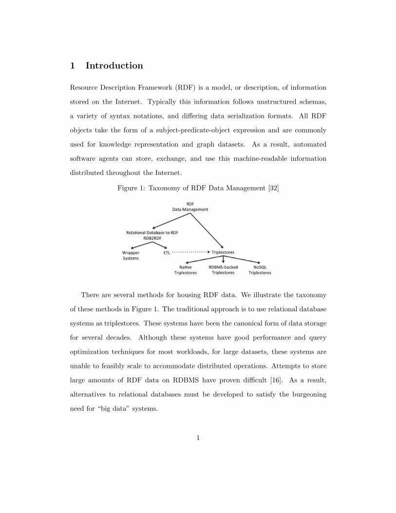
Figure 1: Taxonomy of RDF Data Management [32]

There are several methods for housing RDF data. We illustrate the taxonomy

of these methods in Figure 1. The traditional approach is to use relational database

systems as triplestores. These systems have been the canonical form of data storage

for several decades. Although these systems have good performance and query

optimization techniques for most workloads, for large datasets, these systems are

unable to feasibly scale to accommodate distributed operations. Attempts to store

large amounts of RDF data on RDBMS have proven difficult [16]. As a result,

alternatives to relational databases must be developed to satisfy the burgeoning

need for “big data” systems.

1

In recent years, an alternative class of database systems has emerged. NoSQL

systems, which stand for “not only SQL,” try to solve the scalability limitations

imposed by classical relational systems. Many NoSQL systems attempt to serve

a large number of users simultaneously, efficiently scale to thousands of compute

nodes, and trade full ACID properties for increased performance. Several major

Internet companies such as Google [15], Facebook [35], Microsoft1, and Amazon2

have deployed NoSQL systems in production environments.

In this thesis, we present a NoSQL triplestore used to store and query RDF

data in a distributed fashion. Queries are executed using MapReduce and accept

both SPARQL and SQL languages. This thesis is organized as follows: We begin

with an overview of the technologies used by this system in Section 2. In Section

3, we describe how RDF data is represented and stored in our distributed database

system. Section 4 addresses how we parse and transform SPARQL queries into

MapReduce jobs. Sections 5 and 6 describe our experimental setup, benchmarks,

queries, and query performance followed by a discussion of these results in Section

7. Finally we review related work in Section 8 before concluding in Section 9.

2 Background

2.1 Semantic Web

The Semantic Web was created to enable machines to automatically access and

process a graph of linked data on the World Wide Web. Linked Data refers to

structured data that typically obey following properties [9]: (i) Uniform resource

identifiers, or URIs, uniquely identify things, objects, or concepts. (ii) Each URI

1http://www.windowsazure.com2http://aws.amazon.com

2

points to an HTTP page displaying additional information about the thing or

concept. (iii) Established standards such as RDF and SPARQL are used to structure

information. (iv) Each concept or thing points to another concept or thing using a

URI.

The Resource Description Framework data model structures data into triples

consisting of a subject, predicate, and an object. The subject denotes a thing or

concept, typically a URI. An object can be a literal or a URI, while the predicate

explains the relationship the subject has with the object. Note, that the predicate

need not be reflexive.

RDF data is stored across the Internet as different datasets, each dataset unique

to a specific domain of knowledge. These datasets can be categorized into distributed

datasets or single point-of-access databases [23]. The first of these, distributed

datasets, is often accompanied with a federated query mediator. This mediator is the

entry point for incoming queries. This mediator will then go and fetch the requested

information stored on various websites, databases, and namespaces. Since the data

is stored by the content creators, no additional data infrastructure is required to

store RDF data. However, due to the dependent nature of a distributed dataset, if

a single database (hosted by a third party) is slow or offline, the query execution

time will be negatively affected. An example of a distributed dataset is the FOAF

project [5].

Linked data and the Semantic Web gives both humans and machines additional

search power. By consolidating duplicate information stored in different databases

into a single point-of-access, or centralized cache, we can enable users to perform

faster searches with less external dependencies. Since all information is stored on a

local (single) system, latency can be reduced and queries can execute deterministi-

3

cally. This thesis presents a centralized RDF database system.

2.2 MapReduce

MapReduce [15] is a “programming model and an associated implementation for pro-

cessing and generating large datasets.” It was developed by Jeffrey Dean and Sanjay

Ghemawat at Google as an attempt to streamline large-scale computation processes.

Internet data can be represented in various data formats, both conventional and

unconventional. At Google, this amount of data became so large that processing

this data would require “hundreds or thousands of machines in order to finish in a

reasonable amount of time” [15]. As a result, MapReduce was created to provide

an abstraction of distributed computing and enable programmers to write parallel

programs without worrying about the implementation details such as fault tolerance,

load balancing, and node communication. The most widely used implementation of

the MapReduce framework is Apache Hadoop, described in Section 2.3.

The program being executed is divided into many small tasks which are subse-

quently executed on the various worker nodes. If at any point a sub-task fails, the

task is restarted on the same node or on a different node. In the cluster, a single

master node exists while the remaining nodes are workers. A worker node can be

further classified into mapper nodes and reducer nodes. Mapper nodes perform the

map function while reducer nodes perform the reduce task. We will discuss this

concept in more detail shortly.

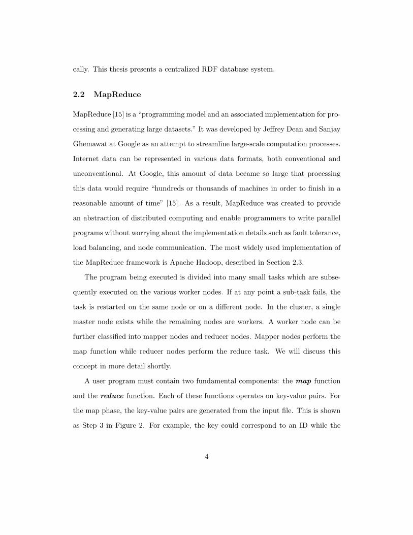
A user program must contain two fundamental components: the map function

and the reduce function. Each of these functions operates on key-value pairs. For

the map phase, the key-value pairs are generated from the input file. This is shown

as Step 3 in Figure 2. For example, the key could correspond to an ID while the

4

Figure 2: Overview of MapReduce Execution [15]

value is a first name. This would give us a key-value pair of 〈ID, First Name〉, e.g.

〈001, John〉, where 〈k,v〉 denotes a key-value pair. The keys nor the values need be

unique. These key-value pairs are then given to the map function which is described

below.

2.2.1 Map Step

In the map step, the master node takes the input key-value pairs, divides it into

smaller sub-problems, and distributes the task to the worker nodes as shown in Step

2 of Figure 2 [1]. Key-value pairs are assigned to worker nodes depending on several

factors such as overall input size, data locality, and the total number of mapper

nodes. In the event where the input file is very large, more specifically, where the

number of input splits is greater than the number of mapper nodes, then the map

jobs will be queued and the mapper nodes will execute the queued jobs sequentially.

5

The worker node then processes the data and emits an intermediate key-value

pair (Steps 3 and 4 of Figure 2). This intermediate key value pair can either be sent

a reducer, if a reduce function is specified, or to the master (and subsequently the

output file), if there is no reduce function.

Algorithm 1 MapReduce Word Count: Map Function

1: function map(String input key, String input value)2: // input key: document/file name3: // input value: document/file contents4: for each word w in input value do5: EmitIntermediate(w,“1”);6: end for7: end function

Algorithm 1 shows an example map function of a MapReduce program. This

particular example counts the number of times each word occurs in a set of files,

documents, or sentences. The input key-value pair is 〈document name, string of

words〉. Each mapper node will parse the list of words and emit a key-value pair for

every word. The key-value pair is 〈word, 1〉. Note that multiple occurrences of the

same word will have the same key-value pair emitted more than once.

2.2.2 Partition and Shuffle Stages

MapReduce guarantees that the input to every reducer is sorted by key [37]. The

process that sorts and transfers the intermediate key-value pairs from mapper to

reducers is called the shuffle stage. The method which selects the appropriate

reducer for each key-value pair is determined by the partition function.

The partition function should give an approximate uniform distribution of data

across the reducer nodes for load-balancing purposes, otherwise the MapReduce

job can wait excessively long for slow reducers. A reducer can be slow due to a

6

disproportionate amount of data sent to it, or simply because of slow hardware.

The default partition function F for both MapReduce and Hadoop is:

F(k, v) : hash(k) mod R

where R is the number of reducers and k is the intermediate key [15, 1]. Once the

reducer has been selected, the intermediate key-value pair will be transmitted over

the network to the target reducer. The user can also specify a custom partition

function. Although not shown in Figure 2, the partition function sorts intermediate

key-value pairs in memory, on each mapper node, before being written to the local

disk. The next step is the shuffle phase.

The shuffle phase consists of each reducer fetching the intermediate key-value

pairs from each of the mappers and locally sorting the intermediate data. Each

reducer asks the master node for the location of the reducer’s corresponding inter-

mediate key-value pairs. Data is then sent across the cluster in a criss-cross fashion,

hence the name shuffle. As the data arrives to the reducer nodes, it is loaded into

memory and/or disk.

Reducers will continue to collect mapper output until the reducers receive a noti-

fication from the JobTracker daemon. The JobTracker process, described in Section

2.3, oversees and maintains between map outputs and their intended reducer. This

process tells the reducer which mapper to ping in order to receive the intermediate

data.

Once all the intermediate key-value pairs have arrived at the reducers, the sort

stage (within the shuffle phase) begins. Note, a more correct term for this phase

would be the merge phase as the intermediate data has already been sorted by

the mappers. After the intermediate data is sorted locally at each reducer, the

reduce step begins. Each reducer can begin this step once it receives its entire task

7

allocation; it need not wait for other reducers.

2.2.3 Reduce Step

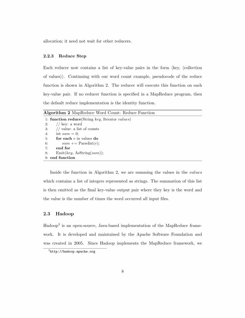
Each reducer now contains a list of key-value pairs in the form 〈key, 〈collection

of values〉〉. Continuing with our word count example, pseudocode of the reduce

function is shown in Algorithm 2. The reducer will execute this function on each

key-value pair. If no reducer function is specified in a MapReduce program, then

the default reduce implementation is the identity function.

Algorithm 2 MapReduce Word Count: Reduce Function

1: function reduce(String key, Iterator values)2: // key: a word3: // value: a list of counts4: int sum = 0;5: for each v in values do6: sum += ParseInt(v);7: end for8: Emit(key, AsString(sum));9: end function

Inside the function in Algorithm 2, we are summing the values in the values

which contains a list of integers represented as strings. The summation of this list

is then emitted as the final key-value output pair where they key is the word and

the value is the number of times the word occurred all input files.

2.3 Hadoop

Hadoop3 is an open-source, Java-based implementation of the MapReduce frame-

work. It is developed and maintained by the Apache Software Foundation and

was created in 2005. Since Hadoop implements the MapReduce framework, we

3http://hadoop.apache.org

8

will describe Hadoop’s two components: the MapReduce engine and the Hadoop

Distribtued File System (HDFS)4.

Before we describe the two components, we will briefly describe the possible roles

a slave node may be assigned:

1. JobTracker - assigns tasks to specific cluster nodes

2. TaskTracker - accepts tasks from JobTracker, manages task progress

3. NameNode - maintains file system, directory tree, and block locations

4. DataNode - stores HDFS data and connects to a NameNode

In small Hadoop clusters, it is common for the master node to perform all

four roles while the slave nodes act as either DataNodes or TaskTrackers. In large

clusters, the DataNode and TaskTracker typically assigned to a dedicated node to

increase cluster throughput.

2.3.1 MapReduce Engine

Hadoop’s MapReduce engine is responsible for executing a user MapReduce pro-

gram. This includes assigning sub-tasks and monitoring their progress. A task is

defined as a map, reduce, or shuffle operation.

The JobTracker is the Hadoop service which assigns specific MapReduce tasks to

specific nodes in the cluster [1]. The JobTracker tries to assign map and reduce tasks

to nodes such that the amount of data transfer is minimized. Various scheduling

algorithms can be used for task assignment. A TaskTracker is a node in the cluster

which accepts tasks from the JobTracker. The TaskTracker will spawn multiple

4The explanation in this section and the remainder of this thesis refers to the Hadoop 1.x release.

9

sub-processes for each task. If any individual task fails, the TaskTracker will restart

the task. Once a task completes, it begins the next task in the queue or will send a

success message to the JobTracker.

2.3.2 Hadoop Distributed File System

The Hadoop Distributed File System (HDFS) is the distributed file system designed

to run on hundreds to thousands of commodity hardware machines [12]. It is highly

fault tolerant and was modeled after the Google File System [21].

HDFS was developed with several goals in mind [4]. Since a Hadoop cluster can

scale to thousands of machines, hardware failures are much more common than in

traditional computing environments. HDFS aims to detect node failures quickly and

automatically recover from any faults or errors. Because of the large cluster size,

HDFS is well-suited for large datasets and can support files with sizes of several

gigabytes to terabytes.

HDFS implements a master/slave architecture. The HDFS layer consists of

a single master, called the NameNode, and many DataNodes, usually one per

machine [4]. Each file is split into blocks, scattered across the cluster, and stored

in DataNodes. DataNodes are responsible for performing the actual read and write

requests as instructed by the NameNode. DataNodes also manage HDFS blocks by

creating, deleting, and replicating blocks.

The NameNode is the head of the HDFS system. The NameNode stores all

HDFS metadata and is responsible for maintaining the file system directory tree

and mapping between a file and its blocks [1]. It also performs global file system

operations such as opening, closing, and renaming files and directories. In the

event the NameNode goes offline, the entire HDFS cluster will fail. It is possible

10

to have a SecondaryNameNode, however this provides intermittent snapshots of the

NameNode. Additionally, automatic failover is not supported and requires manual

intervention in the event of a NamNode failure.

Data replication is an important feature of HDFS. Just as with standard disks,

an HDFS file consists of a sequence of blocks (default size of 64 MB) and are

replicated throughout the cluster. The default replication scheme provides triple

data redundancy but can be modified as needed. The specific placement of these

blocks depends on a multitude of factors but the most significant is a node’s network

rack placement.

2.4 HBase

HBase5 is an open source, non-relational, distributed database modeled after Google

BigTable [13]. It is written in Java and developed by the Apache Software Founda-

tion for use with Hadoop. The goal HBase is to maintain very large tables consisting

of billions of rows and millions of columns [3]. Out of the box, HBase is configured

to integrate with Hadoop and MapReduce.

2.4.1 Data Model

Logically, the fundamental HBase unit is a column [18]. Several columns constitute

a row which is uniquely identified by its row key. We refer to a “cell” as the

intersection of a table row and column. Each cell in the table contains a timestamp

attribute. This provides us with an additional dimension for representing data in

the table.

Columns are grouped into column families which are generally stored together

5http://hbase.apache.org/

11

on disk [3]. The purpose of column families is to group columns with similar access

patterns to reduce network and disk I/O. For example, a person’s demographic

information may be stored in a different column family than their biological and

medical data. When analyzing biological data, demographic information may not

be required. It is important to note that column families are fixed and must be

specified during table creation. To include the column family when identifying table

cells, we use the tuple: value = 〈row key, family : column, timestamp〉.

2.4.2 Architecture

Like Hadoop, HBase implements a master/slave architecture. Tables are partitioned

into regions defined by a starting and ending row key. Each of these regions are

assigned to an HBase RegionServer (slave). The HBase master is responsible for

monitoring all RegionServers and the master is the interface for any metadata

changes [3].

Figure 3: HBase Translation from Logical to Physical Model [20]

In Figure 3, we show the translation from the logical data model to physical

12

representation on disk. In the top left of the figure, an HBase table is shown in its

logical form. Stacked squares coming out of the page represent multiple values with

different timestamps at a cell. Each column family in the table is split into separated

HDFS directories called Stores (top right of Figure 3). Each column family is split

into multiple files on disk called StoreFiles. As shown in the bottom right of the

figure, each row in the file represents a single cell value stored in the HBase logical

model. Each row in the StoreFile contains a key-value pair:

〈key, value〉 = 〈(row key, family : column, timestamp), value〉

Parenthesis have been added for clarity. Depending on the implementation, the

components of the StoreFile key can be swapped without losing information. It is

important to note that swapping the components of the compound key allows for

more complex database implementations without requiring additional disk space.

2.4.3 Selected Features

In this section, we describe some of the advanced features included in HBase, most

of which we use in our system. The features we primarily use are HBase’s bulk

loading tools, bloom filters, and null compression.

Both Hadoop and HBase use the Hadoop Distributed File System. HBase’s

implementation and coordination of internal services is transparent to Hadoop. As

a result, HBase fault tolerance is automatically handled by Hadoop’s data replication

factor while any RegionServer failures are handled by the HBase cluster services.

This simplifies both the setup and management of a Hadoop/HBase cluster.

A very useful feature of HBase is its bulk loading capabilities. As a quick

overview: a MapReduce job transforms some input data into HBase’s internal file

13

format. We take the output file format from this MapReduce job and load it directly

into a live HBase cluster. For specific implementation details and intermediate file

formats, we refer the reader to the HBase bulk loading documentation [2].

Bloom filters allow us to reduce the number of HBase rows read during a table

scan. HBase offers two types of bloom filters: by row and by row+column. When

an HFile is opened, the bloom filter is loaded into memory and used to determine

if a given HBase row key exists in the HFile before scanning the HFile. As a result,

we are able to skip HBase blocks that do not have the requested values.

Depending on the data model used to store RDF, there may be many empty

cells with no values. Because of HBase’s physical model, NULL values use zero disk

space – the key-value for a NULL is simply not written to disk. This differs from

relational databases where NULL values require space for fixed width fields (e.g.

char(10)).

2.5 Hive

Developed by Facebook, Hive6 is a data warehouse and infrastructure built on top

of Hadoop and provides SQL-like declarative language for querying data [35]. It is

now developed by the Apache Software Foundation and supports integration with

HDFS and HBase.

2.5.1 Data Model

Data in Hive is organized into tables, each of which is given a separate directory

on HDFS. However, when used in conjunction with HBase, Hive does not duplicate

the data and instead relies on the data stored on HDFS by HBase. Assuming we

6http://hive.apache.org/

14

have an existing HBase table, a Hive table is created to manage the HBase table.

Creation of a Hive table requires the user to provide a mapping from HBase columns

to Hive columns (line 6 of Codebox 1). This is analogous to creating a SQL view

over a table where the view is stored in Hive while the table is stored in HBase.

Codebox 1: Hive Table Creation with HBase [6]

1 CREATE TABLE

2 hive_table_1(key int , value string)

3 STORED BY

4 ‘org.apache.hadoop.hive.hbase.HBaseStorageHandler ’

5 WITH SERDEPROPERTIES

6 ("hbase.columns.mapping" = ":key ,cf1:val")

7 TBLPROPERTIES

8 ("hbase.table.name" = "xyz");

Since HBase stores sequences of bytes as table values, Hive is unaware of the

data types in the HBase columns. As a consequence, we are required to specify

a primitive type for each Hive column mapping to HBase (line 6 of Codebox 1).

Caution must be taken as it is possible to declare a column of the incorrect type.

Our Hive table being created in Codebox 1 specifies Hive a table referencing two

columns of the HBase table xyz. One column is of type int and points xyz ’s row

keys while the second column points to the column (and column family) cf1:val

represented as strings. Line 3 of Codebox 1 indicates the table we are creating is

stored externally by HBase and will not require storage by Hive. However, Hive

will store metadata such as the Hive-HBase column mapping. The DDL query in

Codebox 1 is executed on Hive to create the table.

15

2.5.2 Query Language and Compilation

Hive provides a SQL-like language called HiveQL as a query language. It is described

as SQL-like because contains some of the features such as equi-joins, but it does not

fully comply with the SQL-92 standard [37].

The concept of a join in a MapReduce environment is the same as the join

operator in a RDBMS. However, the physical plan of a join operator does differ in

a MapReduce environment. There are two broad classes of joins in MapReduce:

(i) map-side join and (ii) reduce-side join. A reduce-side join is a join algorithm in

which the tuples from both relations are compared on their join key and combined

during the reduce phase. A map-side join performs the comparison and combination

during the map phase.

Hive’s default join algorithm is a reduce-side join but it also supports map-side

and symmetric hash joins [39]. Recent releases of Hive have introduced additional

joins such as the Auto MapJoin, Bucket MapJoin, and Skew Join [34]. However,

most of these new algorithms remain map-side joins.

Given an input DDL or DML statement, the Hive compiler converts the string

into a query plan consisting of metadata and/or HBase and HDFS operations. For

insert statements and queries, a tree of logical operators is generated by parsing the

input query. This tree is then passed through the Hive optimizer. The optimized tree

is then converted into a physical plan as a directed acyclic graph of MapReduce jobs

[35]. The MapReduce jobs are then executed in order while pipelining intermediate

data to the next MapReduce job. An example Hive physical plan can be found in

Appendix C.1.

16

3 Data Layer

Before we design the schema, we must first understand the characteristics of RDF

and SPARQL queries so that we know what optimizations are necessary. In Section

3.1, we present a brief analysis of SPARQL queries and characteristics of common

joins. We then describe both our Hive and HBase data model in Section 3.2. In

Section 3.3, we outline how data is manipulated and loaded into the distributed file

system. Finally, we discuss how we employ bloom filters to take advantage of our

schema design in Section 3.4.

3.1 Access Patterns

SPARQL queries access RDF data in many ways. Before we compare and contrast

the different data models, we must first understand the primary use cases of our

database. Listed below are figures from an analysis of 3 million real-world SPARQL

queries on the DBpedia7 and Semantic Web Dog Food8 (SWDF) datasets [19]. We

discuss the results of the study and explain key takeaways which we incorporate

into our schema and data model.

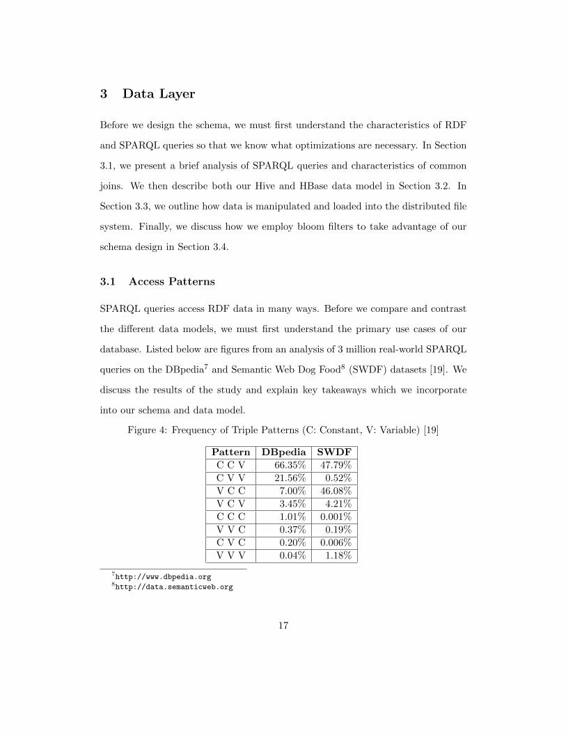
Figure 4: Frequency of Triple Patterns (C: Constant, V: Variable) [19]

Pattern DBpedia SWDF

C C V 66.35% 47.79%

C V V 21.56% 0.52%

V C C 7.00% 46.08%

V C V 3.45% 4.21%

C C C 1.01% 0.001%

V V C 0.37% 0.19%

C V C 0.20% 0.006%

V V V 0.04% 1.18%

7http://www.dbpedia.org8http://data.semanticweb.org

17

Figure 5: Number of Joins and Join Type per Query [19]

We start with the basic analysis of the triple patterns. As shown in Figure 4,

a large percentage of queries have a constant subject in the triple pattern. This

indicates that users are frequently searching for data about a specific subject and

by providing fast access to an HBase row, assuming the row keys are RDF subjects,

we will be able to efficiently serve these queries. Queries with variable predicates

constitute about 22% and 2% of DBpedia and SWDF queries, respectively. This is

more than the percentage of queries with variable subjects. Although variables may

appear in any of the three RDF elements (subject, predicate, object), we must take

care to balance our data model optimizations for each RDF element.

Moving onto an analysis of the queries with joins, in the left graph of Figure

5, we see that 4.25% of queries have at least one join. We define a join as two

triple patterns which share a variable in any of the three RDF positions. Subject-

subject joins constitute more than half of all joins while subject-object constitute

about 35%. Combined with the results from the constant/variable patterns, we

can conclude that subjects are by far the most frequently accessed RDF element.

Therefore, we hypothesize that optimizing the data model for fast access of RDF

18

subjects will allow us to efficiently answer queries requesting subjects and joins

involving subjects.

3.2 Schema Design

There are several data models for representing RDF data which have been studied

and implemented [36, 38, 8]. Taking into account the analysis performed in the

previous section, we employ a property table as our data model. In this section we

will explain our rationale and compare our schema with other models.

A property table derives its name from the logical representation of the table.

Each row contains a key and each column stores some property of that key. Using

HBase as our storage mechanism and Hive as our query engine, we employ a property

table with the following characteristics:

1. Subjects are used as the row key.

2. Predicates are represented as columns.

3. Objects are stored in each cell.

4. Each cell can store multiple values, distinguished by their timestamp.

5. The property table is non-clustered. We use a single property table opposed

to having multiple property tables grouped by similarity.

Our rationale for selecting a property table stems from the shortcomings of tradi-

tional triple-tables. A triple-table is a single table with three columns: a subject

column, predicate column, and object column. Consider the SPARQL query in

Codebox 2. In a triple-table, we must find each subject that satisfied the three graph

patterns specified in the SPARQL query. This requires us to join each subject/row

19

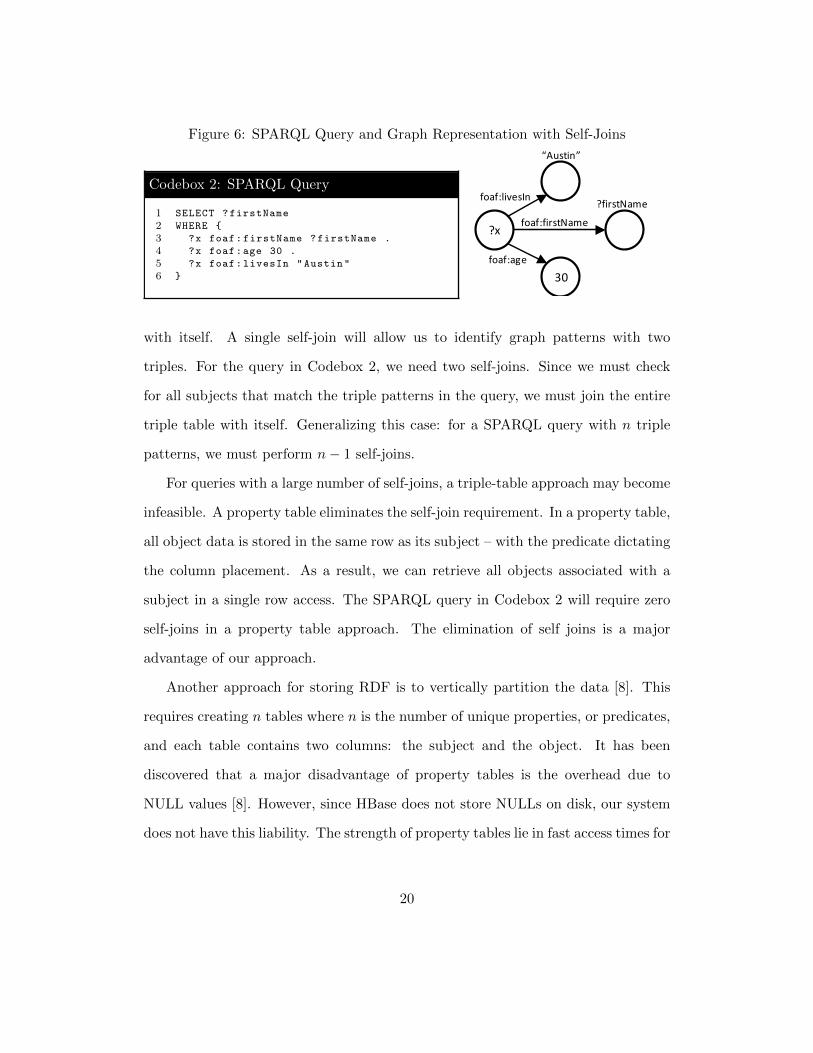
Figure 6: SPARQL Query and Graph Representation with Self-Joins

Codebox 2: SPARQL Query

1 SELECT ?firstName

2 WHERE {

3 ?x foaf:firstName ?firstName .

4 ?x foaf:age 30 .

5 ?x foaf:livesIn "Austin"

6 }

?xfoaf:firstName

30

foaf:age

Austin

foaf:livesIn?firstName

with itself. A single self-join will allow us to identify graph patterns with two

triples. For the query in Codebox 2, we need two self-joins. Since we must check

for all subjects that match the triple patterns in the query, we must join the entire

triple table with itself. Generalizing this case: for a SPARQL query with n triple

patterns, we must perform n− 1 self-joins.

For queries with a large number of self-joins, a triple-table approach may become

infeasible. A property table eliminates the self-join requirement. In a property table,

all object data is stored in the same row as its subject – with the predicate dictating

the column placement. As a result, we can retrieve all objects associated with a

subject in a single row access. The SPARQL query in Codebox 2 will require zero

self-joins in a property table approach. The elimination of self joins is a major

advantage of our approach.

Another approach for storing RDF is to vertically partition the data [8]. This

requires creating n tables where n is the number of unique properties, or predicates,

and each table contains two columns: the subject and the object. It has been

discovered that a major disadvantage of property tables is the overhead due to

NULL values [8]. However, since HBase does not store NULLs on disk, our system

does not have this liability. The strength of property tables lie in fast access times for

20

multiple properties regarding the same subject. In a vertically partitioned datastore,

the SPARQL query in Codebox 2 would require accessing three different tables and

require joins.

The Hexastore approach for storing RDF builds six indices, one for each of

the possible ordering of the three RDF elements [36]. Queries are executed in

the microsecond range and outperform other RDF systems by up to five orders

of magnitude. Although Hexastore has stellar performance, it requires indices

to be constructed and stored in memory. As the dataset size increases, memory

usage increases linearly. As a result, memory usage becomes the limiting factor of

Hexastore’s ability to accommodate large datasets. For this reason, we do not adopt

the Hexastore approach.

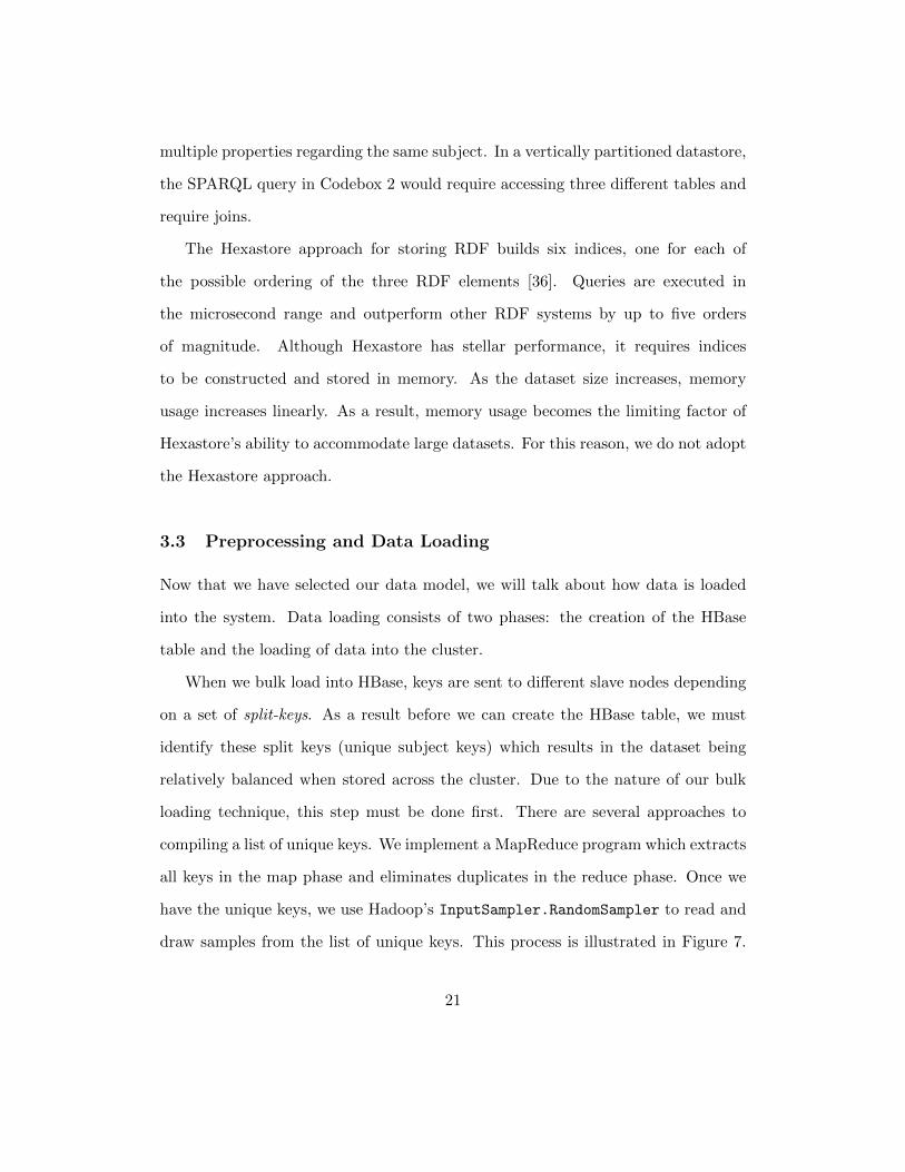
3.3 Preprocessing and Data Loading

Now that we have selected our data model, we will talk about how data is loaded

into the system. Data loading consists of two phases: the creation of the HBase

table and the loading of data into the cluster.

When we bulk load into HBase, keys are sent to different slave nodes depending

on a set of split-keys. As a result before we can create the HBase table, we must

identify these split keys (unique subject keys) which results in the dataset being

relatively balanced when stored across the cluster. Due to the nature of our bulk

loading technique, this step must be done first. There are several approaches to

compiling a list of unique keys. We implement a MapReduce program which extracts

all keys in the map phase and eliminates duplicates in the reduce phase. Once we

have the unique keys, we use Hadoop’s InputSampler.RandomSampler to read and

draw samples from the list of unique keys. This process is illustrated in Figure 7.

21

For small datasets it may be possible to do this sequentially on a single machine,

however, for large datasets, it is recommended to process the input in parallel. We

use the following parameters for the InputSampler.RandomSampler:

1. The probability with which a key will be chosen is 10%.

2. The total number of samples to obtain is 10% of the number of keys.

3. The maximum number of sampled input file-splits is 50%.

We have found that the above parameters balance accuracy and compute time. The

InputSampler.RandomSampler will output a list of sorted keys. We take this list

of keys and select 2, 4, 8, or 16 keys that evenly split the list into partitions. These

become the split-keys. We use powers of two since those are the number of nodes

used in our experiment. When creating the HBase table, we give these split-keys as

additional parameters. The effect of providing these keys to HBase become apparent

during the next phase: loading the data into the table.

Loading data into HBase is a two step process. First, we must create a set

of files which match HBase’s internal storage format. We do this with a custom

MapReduce job. However, other methods are provided by HBase which allow

various input formats [2]. Inside our MapReduce program, we parse the input file

and perform various transformations to the dataset. One of these transformations

includes compressing all URIs using their corresponding namespace prefix.

Another critical transformation is converting special RDF data types to primitive

types. Datasets may include non-primitive types such as longitude, elevation, and

hour. Due to the unstructured representation of RDF data, data type information

is included in the RDF object itself (of type string) as shown below:

"6"^^<http://www.w3.org/2001/XMLSchema#integer>

22

Figure 7: HBase Key Generation

Map Map Map

Raw Dataset on HDFS

Reduce Reduce Reduce

Sorted Unique Keys (Subjects)

Create HBase Table

RandomSampler Split Keys

Figure 8: HFile Creation and Upload

Hbase RegionServers

Map Map Map

Raw Dataset on HDFS

Reduce Reduce Reduce

HFile HFile HFileHFile HFileHFile

a-f g-m n-z A-T U-9

When we convert from the above string to a primitive type, we must remove

the additional information from the string itself and infer its primitive type. It

is important to note we are not losing this information as we are including this

information as the RDF object’s type, which is later used by Hive. The transformed

object becomes 6 of type integer. In the event the Hive or HBase system loses the

type information, a mapping of predicates to predicate types is also maintained and

written to disk.

The above transformations are done in the map phase which outputs an HBase

Put. A Put is HBase’s representation of a pending value insertion. Conveniently by

the inherent nature of MapReduce, all Puts for a single subject are sent to the same

reducer since key-value pairs are sorted on the key (subject). The reduce phase

inserts the Puts into an HFile. An HFile is HBase’s internal data storage format.

The final phase of bulk loading requires moving the HFiles to the appropriate

23

HBase RegionServers, as shown in Figure 8. HBase does this by iterating through the

output HFiles generated by the MapReduce job located on HDFS. HBase compares

the first key in the HFile and determines which RegionServer it belongs to. This

mapping between keys and RegionServers is determined by the split-keys generated

previously and HBase table metadata (Figure 7). The entire bulk loading process

can be performed on a live Hadoop/HBase cluster. Once the above steps are

complete, the data becomes live in HBase and is ready to be accessed.

We have explained the preprocessing required when loading data into HBase.

This included two steps: (i) identifying the set of HBase region split-keys and (ii)

transforming the input data according to a set of rules and moving the data into

the RegionServers.

3.4 Bloom Filters

As mentioned in Section 2.4.3, HBase allows the use of bloom filters. A bloom filter

is a probabilistic data structure used to test if an element is part of a set or not.

Usually represented as a bit vector, it returns “possibly in the set” or “definitely

not in the set” [11]. The bits in the vector are set to 0 or 1 depending on a set of

hash functions applied to the element being added/searched in the bloom filter.

Each HFile (or block), represents a fragment of an HBase table. Each block is

equipped with a bloom filter. As a result, we are able to quickly check whether a

table value exists in block or not. Upon inserting data into HBase, we hash the row

key and column as a compound hash key (in RDF terms, the subject and predicate),

and populate our bloom filter. When searching for RDF triples in the HBase table,

we hash the subject and predicate and check the bloom filter. The bloom filter will

tell us whether an RDF object exists in the block with the (hashed) subject and

24

predicate. If the bloom filter tells us no, then we skip reading the current block.

We can achieve greater gains from the use of bloom filters through our bulk

loading process with MapReduce. If MapReduce was not used for bulk loading

and data was inserted randomly (data is generally sorted randomly in input files),

then all triples for a specific subject “albert” will be scattered throughout many

blocks across the HDFS cluster. We define an “albert” triple an RDF triple with

“albert” as the subject. When scanning the HBase table, we would see many true

results from our bloom filters since the “albert” triples lie in many HDFS blocks.

By using MapReduce, data is sorted before the reduce stage and therefore all triples

with “albert” as the subject will be sent to the same reducer and as a result, be

written to the same HFiles. This allows our bloom filters to return true for these

“albert”-triple concentrated files and return false for the other HDFS blocks.

Additionally, by using a compound hash key consisting of the row key and

column, we can further reduce the number of blocks read. HBase offers two types

of bloom filters with different hash keys: (i) row key only as the hash key and

(ii) row key concatenated with the column. Continuing from our previous example

with “albert” triples, assume all “albert” triples lie in two blocks. Consider the

case where we are looking for the city “albert” lives in (denoted by the predicate

“livesInCity”). Note that there is only one possible value for the object because

a person can only live in one city at a time. If we employ a row-key-only bloom

filter, then the bloom filter will return true for both blocks and we must scan both.

However, if we use a row key and column hash, then the bloom filter will return

false for one block and true for the other – further reducing the number of blocks

read. This feature is especially useful for predicates with unique value as there is

only one triple in the entire database with the value we require. In the ideal case,

25

bloom filters should allow us to read only a single HFile from disk. However, due

to hash collisions and false positives, this may not be achieved.

The above techniques allow us to accelerate table scans and by skipping irrelevant

HDFS blocks. In the next section, we describe how we use Hive to query data stored

in HBase.

4 Query Layer

We use Apache Hive to execute SPARQL queries over RDF data stored in HBase.

Several processes must completed before the query is executed as a MapReduce job.

In Section 4.1, we describe how the query is reformulated to leverage the advantages

created by our property table design. This requires creating intermediate views

described in Section 4.2. From there we build the abstract syntax tree in Section

4.3. The final component of the query layer is the HiveQL generator, which we

discuss in Section 4.4.

4.1 Join Conditions

We define a join as the conjunction of two triple patterns that share a single variable

in different RDF positions – specifically, a variable in the subject position and a

variable in the object position. This is different from the analysis performed in

Section 3.1. Triple patterns that share the same variable subject do not require a

join in our data model due to the nature of property tables. The SPARQL query

defines a set of triple patterns in the WHERE clause for which we are performing a

graph search over our database and identifying matching subgraphs. In order to

utilize the features of the property table, we must first group all triple patterns with

the same subject. Each group will become a single Hive/HBase row access. This

26

is done in three steps. We explain the process of identifying a join query using the

query in Codebox 3, also depicted as a graph in Figure 10.

Codebox 3: Join Query (SPARQL)

1 PREFIX foaf: <http :// xmlns.com/foaf /0.1/ >

2 PREFIX rdf: <http ://www.w3.org /1999/02/22 -rdf -syntax -ns#>

34 SELECT ?firstName , ?age , ?population

5 WHERE {

6 ?x foaf:firstName ?firstName .

7 ?x foaf:age ?age .

8 ?x rdf:type rdf:Person .

9 ?x foaf:livesIn ?country .

10 ?country foaf:population ?population

11 }

First, we must group all triple patterns in the SPARQL WHERE clause by subject.

The query in Codebox 3 conveniently satisfies this property by default. We then

iterate through the triple patterns and create a list of unique subjects that are being

referenced. In Codebox 3, our list of unique subjects, L, contains two elements:

L = {?x, ?country}. In the event we have the same constant subject occurring

in two different positions in two triple patterns, we must perform a join. This is

demonstrated in Codebox 4. Using L, we create a mapping such that each unique

subject S∗ ∈ L maps to a list of triple patterns of the form 〈S∗, P,O〉. The result is

a map M with KeySet(M) = L, shown in Figure 9.

Figure 9: Mapping of Query Subjects to Triple Patterns

?x

?country

?x foaf:firstName ?firstName?x foaf:age ?age?x rdf:type rdf:Person?x foaf:livesIn ?country

?country foaf:population ?population

KeySet Values (Triple Patterns)

27

Figure 10: Join Query (Graph Form)

?xlivesIn

?country

type

age

rdf:Person

?age

?population?firstName

hasPopulation

firstName

Figure 11: Join Query (Join Condition)

?xlivesIn

?country

type

age

rdf:Person

?age

?population?firstName

hasPopulation

firstName

Second, we must check if any two triple patterns in the WHERE clause have the

form 〈S1P1O1〉 and 〈S2P2O2〉 where O1 = S2. This is done by iterating through

all triple patterns in our mapping. For each triple pattern, we check if the object

matches any object in our list of unique subjects, KeySet(M). If a triple pattern,

〈S, P,O〉, contains an O ∈ KeySet(M), then we know that a join must be performed

on S and O. Figure 11 illustrates the mapping in Figure 9 in graph form. The

different node colorings represent the different objects being referenced by a specific

subject. The dashed line represents line 9 of Codebox 3 which is the triple pattern

indicating a join is necessary. In our property table model, this requires a join. In

other data models, a join may not be required and may not be caused by line 9. We

summarize the process for identifying a join condition: Let S be a subject in the

query Q. Let N be the number of triple patterns in the WHERE clause of the query.

Let: M : S → {〈S, P1, O1〉, ..., 〈S, Pn, On〉}, n ≤ N . A SPARQL query will require a

join in our system if the SPARQL WHERE clause satisfies the following properties:

1. |KeySet(M)| ≥ 2

2. ∃〈S1, P1, O1〉, 〈S2, P2, O2〉 ∈ Q such that(O1 = S2

)∧(S1, S2 ∈ KeySet(M)

)

28

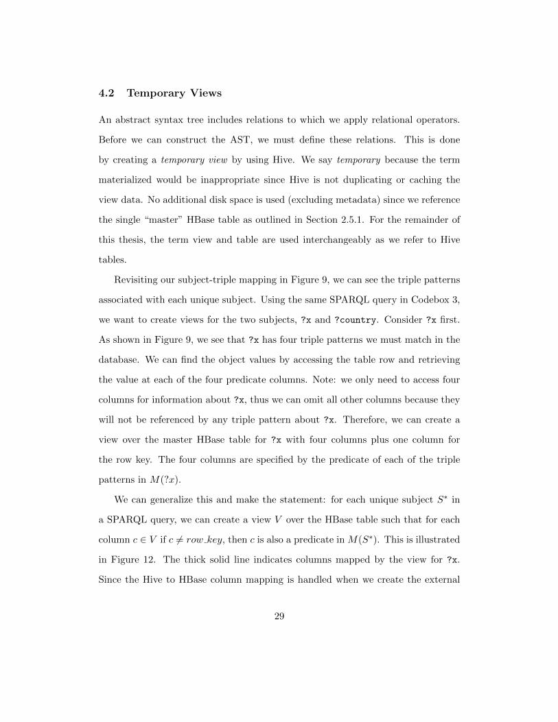
4.2 Temporary Views

An abstract syntax tree includes relations to which we apply relational operators.

Before we can construct the AST, we must define these relations. This is done

by creating a temporary view by using Hive. We say temporary because the term

materialized would be inappropriate since Hive is not duplicating or caching the

view data. No additional disk space is used (excluding metadata) since we reference

the single “master” HBase table as outlined in Section 2.5.1. For the remainder of

this thesis, the term view and table are used interchangeably as we refer to Hive

tables.

Revisiting our subject-triple mapping in Figure 9, we can see the triple patterns

associated with each unique subject. Using the same SPARQL query in Codebox 3,

we want to create views for the two subjects, ?x and ?country. Consider ?x first.

As shown in Figure 9, we see that ?x has four triple patterns we must match in the

database. We can find the object values by accessing the table row and retrieving

the value at each of the four predicate columns. Note: we only need to access four

columns for information about ?x, thus we can omit all other columns because they

will not be referenced by any triple pattern about ?x. Therefore, we can create a

view over the master HBase table for ?x with four columns plus one column for

the row key. The four columns are specified by the predicate of each of the triple

patterns in M(?x).

We can generalize this and make the statement: for each unique subject S∗ in

a SPARQL query, we can create a view V over the HBase table such that for each

column c ∈ V if c 6= row key, then c is also a predicate in M(S∗). This is illustrated

in Figure 12. The thick solid line indicates columns mapped by the view for ?x.

Since the Hive to HBase column mapping is handled when we create the external

29

Figure 12: Hive View Generation

Key (Subject) rdf:type foaf:firstName foaf:age rdfs:description foaf:gender foaf:population foaf:livesIn

…

Person1 rdf:Person Bob 57 Male United States

…

United States 314,000,000

…

Person2 rdf:Person Jane 55 Female United States

China 1,351,000,000

Person3 rdf:Person Angela 21 Female China

…

France 65,700,000

Key (Subject) rdf:type foaf:firstName foaf:age foaf:livesIn Key (Subject) foaf:population

… …

Person1 rdf:Person Bob 57 United States Person1

… …

United States United States 314,000,000

… …

Person2 rdf:Person Jane 55 United States Person2

China China 1,351,000,000

Person3 rdf:Person Angela 21 China Person3

… …

France France 65,700,000

Key foaf:firstName rdf:type foaf:age foaf:livesIn foaf:population

Person1 Bob 57 United States 314,000,000

Person2 Jane 55 United States 314,000,000

Person3 Angela 21 China 1,351,000,000

Hive Table R2: View for ?countryHive Table R1: View for ?x

Master Table on HBase

Resulting Hive Table: R1 JOIN R2 ON (R1.foaf:livesIn = R2.key)

Hive table, these columns need not be adjacent in HBase. In this view, we see the

four predicates in the SPARQL query that have ?x as their subject. Since ?x is a

variable, ?x assumes the value of the row key. We apply this same process to the

view for ?country. We index each subject in KeySet(M) with an integer and create

the corresponding Hive table named after the integer index. For example, R2 refers

to the view for ?country. Hive performs the join and we see the joined relation at

the bottom of the figure. The columns with a double border are projected as the

final query result.

30

While the SPARQL/Hive query is being executed, the views consume disk space

for metadata. Once the query completes, all views are discarded and their metadata

is deleted. It is possible for the views to persist but since each view contains a

mapping to HBase columns for a unique SPARQL query, it is unlikely that future

queries will reference the exact same data.

By nature of SPARQL, given a specific subject and predicate, it is possible

for multiple objects to exist. In HBase, these objects are distinguished by their

timestamp value. Since Hive does not support cell-level timestamps, we store

multivalued attributes in Hive’s array data type. The default data type for Hive

columns are strings. For numeric types, the system checks the predicate-primitive

type mapping (see Section 3.3) before creating the Hive view.

The primary benefit of applying the relational concept of views to Hive is the

reduction of information processed by Hadoop/MapReduce. By using Hive, we are

able to perform a relational project on the underlying HBase table and exclude

irrelevant information to the SPARQL query. Views serve as an optimization by

reducing data processed by mapper nodes and by reducing data shuffled by the

network.

4.3 Abstract Syntax Tree Construction

Given the subject-triple pattern mapping M described in the previous section, we

are almost ready to construct the abstract syntax tree. The remaining step is to

identify the Hive columns associated with the remaining variables. Continuing our

example in Codebox 3, we must assign a Hive column to ?population, ?age, and

?firstName. This is easily done by looking at the predicate for that triple pattern.

?firstName is the data stored in the column foaf:firstName, ?age is the column

31

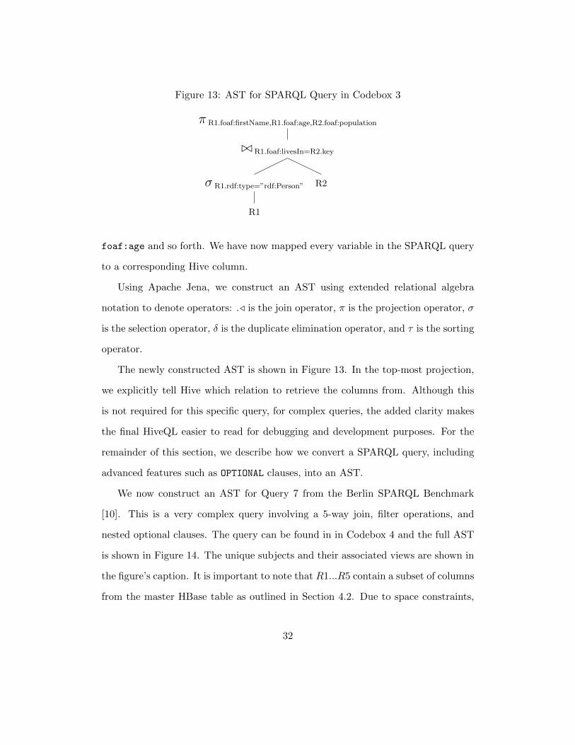
Figure 13: AST for SPARQL Query in Codebox 3

π R1.foaf:firstName,R1.foaf:age,R2.foaf:population

./ R1.foaf:livesIn=R2.key

σ R1.rdf:type=”rdf:Person”

R1

R2

foaf:age and so forth. We have now mapped every variable in the SPARQL query

to a corresponding Hive column.

Using Apache Jena, we construct an AST using extended relational algebra

notation to denote operators: ./ is the join operator, π is the projection operator, σ

is the selection operator, δ is the duplicate elimination operator, and τ is the sorting

operator.

The newly constructed AST is shown in Figure 13. In the top-most projection,

we explicitly tell Hive which relation to retrieve the columns from. Although this

is not required for this specific query, for complex queries, the added clarity makes

the final HiveQL easier to read for debugging and development purposes. For the

remainder of this section, we describe how we convert a SPARQL query, including

advanced features such as OPTIONAL clauses, into an AST.

We now construct an AST for Query 7 from the Berlin SPARQL Benchmark

[10]. This is a very complex query involving a 5-way join, filter operations, and

nested optional clauses. The query can be found in in Codebox 4 and the full AST

is shown in Figure 14. The unique subjects and their associated views are shown in

the figure’s caption. It is important to note that R1...R5 contain a subset of columns

from the master HBase table as outlined in Section 4.2. Due to space constraints,

32

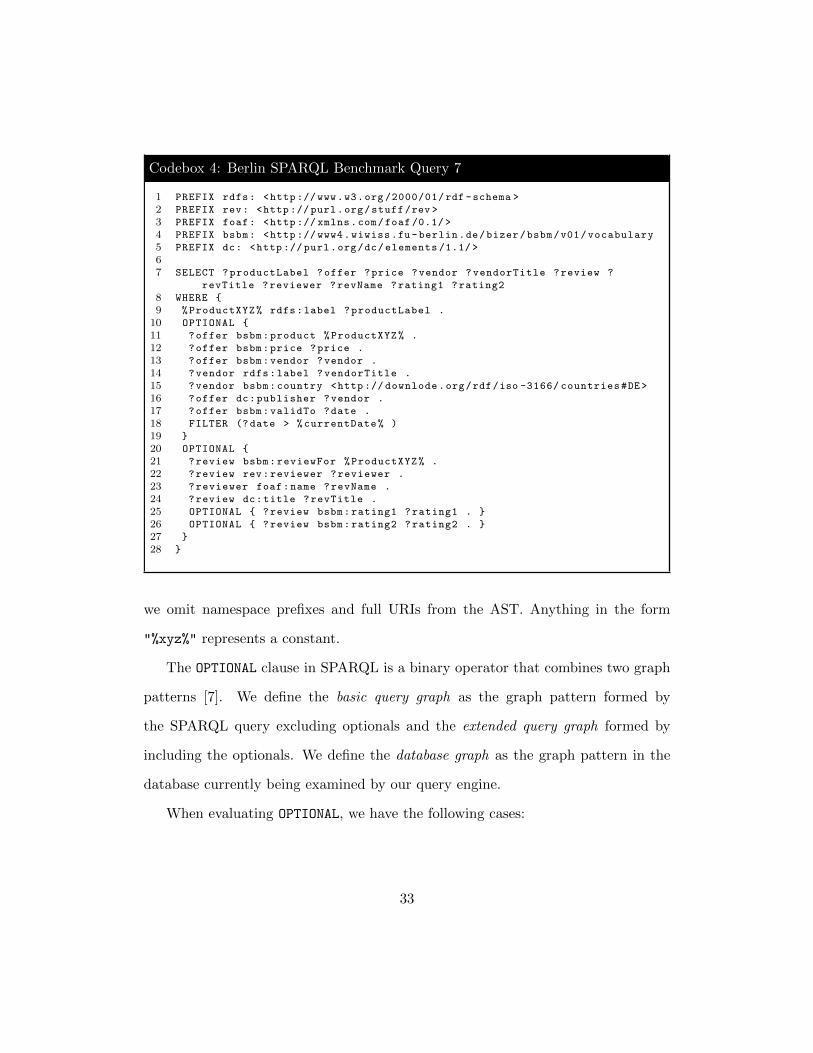
Codebox 4: Berlin SPARQL Benchmark Query 7

1 PREFIX rdfs: <http :// www.w3.org /2000/01/rdf -schema >

2 PREFIX rev: <http :// purl.org/stuff/rev >

3 PREFIX foaf: <http :// xmlns.com/foaf /0.1/ >

4 PREFIX bsbm: <http :// www4.wiwiss.fu-berlin.de/bizer/bsbm/v01/vocabulary

5 PREFIX dc: <http :// purl.org/dc/elements /1.1/ >

67 SELECT ?productLabel ?offer ?price ?vendor ?vendorTitle ?review ?

revTitle ?reviewer ?revName ?rating1 ?rating2

8 WHERE {

9 %ProductXYZ% rdfs:label ?productLabel .

10 OPTIONAL {

11 ?offer bsbm:product %ProductXYZ% .

12 ?offer bsbm:price ?price .

13 ?offer bsbm:vendor ?vendor .

14 ?vendor rdfs:label ?vendorTitle .

15 ?vendor bsbm:country <http :// downlode.org/rdf/iso -3166/ countries#DE>

16 ?offer dc:publisher ?vendor .

17 ?offer bsbm:validTo ?date .

18 FILTER (?date > %currentDate% )

19 }

20 OPTIONAL {

21 ?review bsbm:reviewFor %ProductXYZ% .

22 ?review rev:reviewer ?reviewer .

23 ?reviewer foaf:name ?revName .

24 ?review dc:title ?revTitle .

25 OPTIONAL { ?review bsbm:rating1 ?rating1 . }

26 OPTIONAL { ?review bsbm:rating2 ?rating2 . }

27 }

28 }

we omit namespace prefixes and full URIs from the AST. Anything in the form

"%xyz%" represents a constant.

The OPTIONAL clause in SPARQL is a binary operator that combines two graph

patterns [7]. We define the basic query graph as the graph pattern formed by

the SPARQL query excluding optionals and the extended query graph formed by

including the optionals. We define the database graph as the graph pattern in the

database currently being examined by our query engine.

When evaluating OPTIONAL, we have the following cases:

33

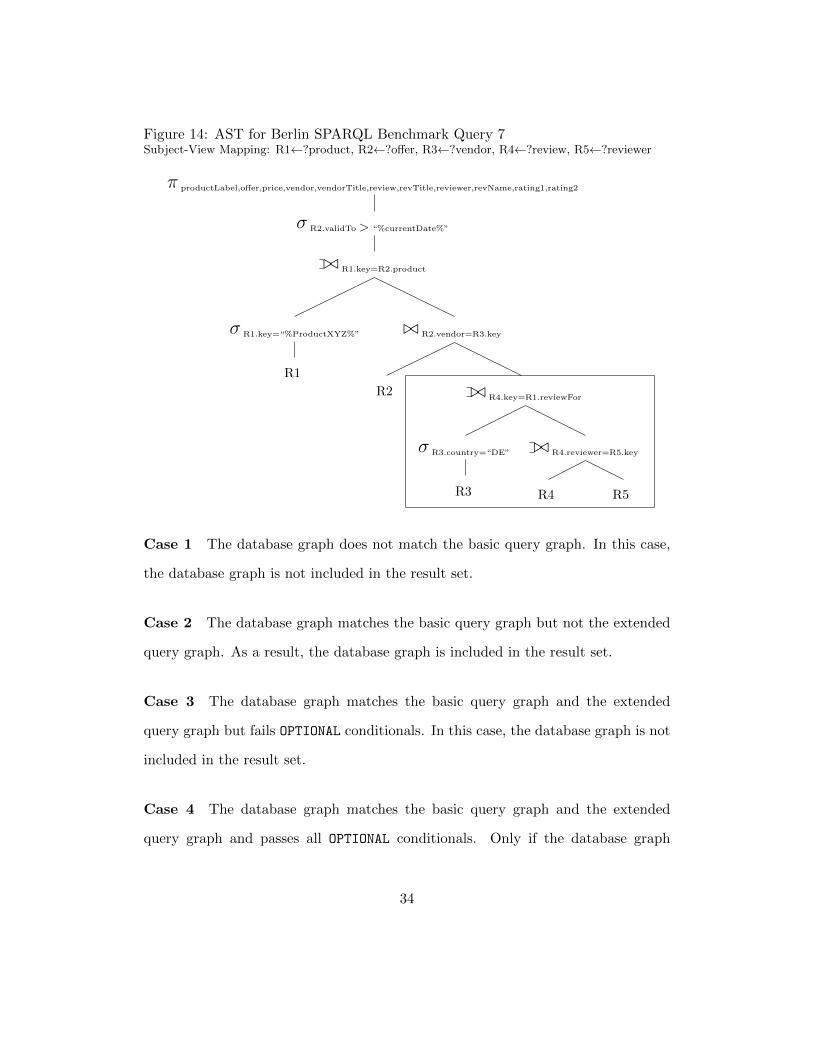
Figure 14: AST for Berlin SPARQL Benchmark Query 7Subject-View Mapping: R1←?product, R2←?offer, R3←?vendor, R4←?review, R5←?reviewer

π productLabel,offer,price,vendor,vendorTitle,review,revTitle,reviewer,revName,rating1,rating2

σ R2.validTo > “%currentDate%”

./ R1.key=R2.product

σ R1.key=“%ProductXYZ%”

R1

./ R2.vendor=R3.key

R2 ./ R4.key=R1.reviewFor

σ R3.country=“DE”

R3

./ R4.reviewer=R5.key

R4 R5

Case 1 The database graph does not match the basic query graph. In this case,

the database graph is not included in the result set.

Case 2 The database graph matches the basic query graph but not the extended

query graph. As a result, the database graph is included in the result set.

Case 3 The database graph matches the basic query graph and the extended

query graph but fails OPTIONAL conditionals. In this case, the database graph is not

included in the result set.

Case 4 The database graph matches the basic query graph and the extended

query graph and passes all OPTIONAL conditionals. Only if the database graph

34

satisfies everything, then we return the database graph in the result set.

In the traditional relational model, Case 4 can be accommodated with an outer

join. Because most SPARQL queries specify the required graph patterns before

the optional patterns, it is common for left outer joins to be used. This is best

illustrated by the boxed subtree in Figure 14. Both R4 and R5 contain information

about reviews and reviewers. Since no filter is applied to R4 or R5, we return all

values. However, when we perform a filter on the R3 (vendors) we must remove non-

German (DE) countries. If a vendor has no country listed, we must not remove them

from the result set. The selection σR2.validTo > “%currentDate%” appears at the top

of the tree because Hive only supports equality conditionals within a join condition.

We traverse the AST and check if any non-equality condition appears below a join

– usually a selection operator. We then move the operator to appear above the

joins in the AST. Logically and syntactically, these selections are performed after

the joins complete.

Given the AST, we can then perform additional transformations or optimizations

such as attribute renaming or selection push-down. Since the AST resembles a

traditional relational AST, we can apply the same set of RDBMS optimization rules

to our translator. Since this system is in its early stages, we do not include a full-

fledged optimizer but instead optimize selection placement in the AST. As shown

in Figure 14, all equality selections occur before any joins are performed.

4.3.1 Additional SPARQL Operators

The Berlin Query 7 demonstrates use of the FILTER and heavy use of the OPTIONAL

keyword. Our parser and AST generator account for other SPARQL operators as

well. For the remainder of this section, we outline the process for identifying each

35

operator and its operands, how we transform it into relational algebra, and emit the

correct HiveQL code. The additional features we support are: ORDER BY, FILTER

(with regular expressions), DESCRIBE, LIMIT, UNION, REDUCED, and BOUND.

ORDER BY. Located near towards the end of each SPARQL query, the ORDER BY

clause appears at the top of the AST, denoted by τ . In Figure 14, if an ORDER BY

was present in the SPARQL, it would be represented as τcolumn and be the parent

of π. In SPARQL, ORDER BY operates on a variable. Using the same process as

for identifying projected columns for the SELECT, we use the subject-triple pattern

mapping to identify which Hive column to sort by.

FILTER. We represent the SPARQL regular expression FILTER as a selection σ

in the AST to conform with standard relational algebra. The regex string is used

as the argument for σ. While in AST form, FILTER by regex is handled the same

as a non-regex FILTER. They remain the same until we differentiate the two during

generation of HiveQL where the regex filter is emitted as a LIKE.

DESCRIBE. This is equivalent to a SELECT ALL in standard SQL. We represent

this in the AST as a projection π where we project all columns in our property

table. This is an expensive operation since we must access all columns in our Hive

table which are scattered throughout HDFS.

LIMIT. This occurs at the end of the SPARQL query. It is not supported by

relational algebra and as a consequence, it is not represented in our AST. When

generating HiveQL, we must manually check the original SPARQL query for the

existence of this operator. This is described in more detail when we generate HiveQL.

UNION. Unions in SPARQL combine two relations or subquery results. Repre-

senting this in our AST requires two subqueries, with identically projected columns

before the union occurs. To do this, we recurse into each of the SPARQL UNION

36

relations and perform the same process as if we started with a brand new SPARQL

query. This will result in two subqueries projecting identical columns. Hive views

will be created as necessary by each of the subqueries. The view generation process

is identical to generating views in the primary (outer) query.

REDUCED. This operator is used as a hint to the query engine. It indicates that

duplicates can be eliminated but it is not required. In our system’s query engine,

we abide by all REDUCED requests and remove duplicates. It is represented in our

AST by a duplicate elimination operator δ. No operands are required.

BOUND. This operator requires a single variable as an operand. As defined in

SPARQL, this operator returns true if the variable is bound (i.e. is not null) and

false otherwise. The BOUND operator translates to a selection σ where the bound

variable is not null. To find the specific column to which the variable is referring to,

we use the subject-triple pattern mapping shown in Figure 9.

The next section outlines how we generate the HiveQL statement using the

original SPARQL query and newly generated AST.

4.4 HiveQL Generation

The final step is to generate the HiveQL query which will be executed on Hive,

HBase, and MapReduce. We have done most of the work and simply need to put

it in HiveQL (SQL) form. The remaining steps require specifying which relation

the projection attributes will be retrieved from. We will continue with both of our

example queries: the simple join query in Codebox 3 and the complex Berlin Query

7 in Codebox 4. We will focus on the join query first.

Using the newly constructed AST in Figure 13, we begin generating HiveQL

from the root node. We see the root node is a projection and thus go to the

37

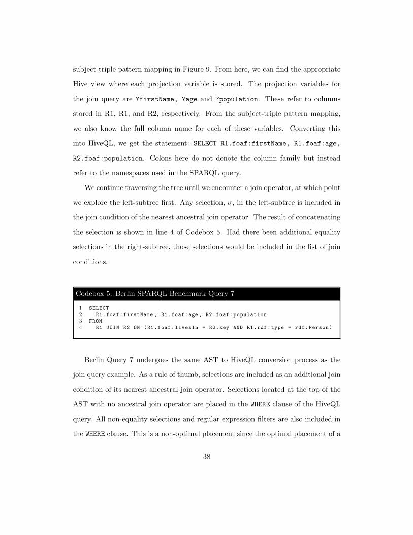
subject-triple pattern mapping in Figure 9. From here, we can find the appropriate

Hive view where each projection variable is stored. The projection variables for

the join query are ?firstName, ?age and ?population. These refer to columns

stored in R1, R1, and R2, respectively. From the subject-triple pattern mapping,

we also know the full column name for each of these variables. Converting this

into HiveQL, we get the statement: SELECT R1.foaf:firstName, R1.foaf:age,

R2.foaf:population. Colons here do not denote the column family but instead

refer to the namespaces used in the SPARQL query.

We continue traversing the tree until we encounter a join operator, at which point

we explore the left-subtree first. Any selection, σ, in the left-subtree is included in

the join condition of the nearest ancestral join operator. The result of concatenating

the selection is shown in line 4 of Codebox 5. Had there been additional equality

selections in the right-subtree, those selections would be included in the list of join

conditions.

Codebox 5: Berlin SPARQL Benchmark Query 7

1 SELECT

2 R1.foaf:firstName , R1.foaf:age , R2.foaf:population

3 FROM

4 R1 JOIN R2 ON (R1.foaf:livesIn = R2.key AND R1.rdf:type = rdf:Person)

Berlin Query 7 undergoes the same AST to HiveQL conversion process as the

join query example. As a rule of thumb, selections are included as an additional join

condition of its nearest ancestral join operator. Selections located at the top of the

AST with no ancestral join operator are placed in the WHERE clause of the HiveQL

query. All non-equality selections and regular expression filters are also included in

the WHERE clause. This is a non-optimal placement since the optimal placement of a

38

selections is before a join operator. However, Hive places this restriction on HiveQL

queries.

Regular expression comparisons are denoted in HiveQL by using the LIKE oper-

ator. During the AST traversal, any selection containing a reserved regex symbol

will be marked as a regex filter. As a result, the HiveQL generator will emit a

HiveQL fragment with LIKE. Both non-equality and regex filters are placed in the

WHERE clause as an additional condition.

Abstract syntax trees with more than one join are denoted as an n-way join.

Joins are appended to the HiveQL query by AST level first, then by left-to-right.

The resulting HiveQL for the Berlin Query 7 is shown in Codebox 6.

Codebox 6: Berlin SPARQL Benchmark Query 7 as HiveQL

1 SELECT

2 R1.label , R2.key , R2.price , R2.vendor , R3.label , R4.key , R4.title ,

3 R4.reviewer , R5.name , R4.rating1 , R4.rating2

4 FROM

5 R1 LEFT OUTER JOIN R2 ON (R1.key="%ProdXYZ%" AND R1.key=R2.product)

6 JOIN R3 ON (R2.vendor = R3.key)

7 LEFT OUTER JOIN R4 ON (R4.key = R1.reviewFor)

8 LEFT OUTER JOIN R5 ON (R4.reviewer = R5.key)

9 WHERE

10 R3.country = "<http :// downlode.org/rdf/iso -3166/ countries#DE >"

11 AND R2.validTo > %currentDate%

Left outer joins are handled the same way as natural joins. Because of our

parsing strategy, full- and right-outer joins do not occur in our AST and will not

appear in the HiveQL query.

Unions are placed in the HiveQL WHERE clause with two subqueries. Each

subquery is given its own set of Hive views from which the subquery is executed

on. The Hive views must remain separate and are assigned different view names

in the HiveQL query. The SPARQL BOUND is placed in the HiveQL WHERE clause

39

as an IS NOT NULL. The DISTINCT and REDUCED keywords are placed immediately

following SELECT but before the list of projected columns. Any limits or ordering

requirements are placed at the end of the HiveQL query.

Once the HiveQL generator has evaluated every node of the AST, the HiveQL

query is then constructed as a single string and executed on Hive. Hive generates

a physical query plan (see Appendix C.1) and begins execution of the MapReduce

jobs. Once all jobs have completed, all materialized views are discarded, the result

is returned as XML, and the query is complete.

5 Experimental Setup

In our NoSQL system, many techniques were borrowed from relational database

management systems. Since the primary aim of this system is to cache the Semantic

Web by storing massive amounts of RDF data, we must analyze the performance in

a cloud setting. To evaluate this system, we perform several benchmark tests in a

distributed environment. The benchmarks used in the evaluation are described in

Section 5.1, the computational environment is outlined in Section 5.2, and system

settings in Section 5.3. Results are presented in Section 6 followed by a discussion

in Section 7.

5.1 Benchmarks

Two benchmarks were used in the evaluation of the system: the Berlin SPARQL

Benchmark (BSBM) and the DBpedia SPARQL Benchmark. Both of these bench-

marks are freely available online for download.

40

5.1.1 Berlin SPARQL Benchmark

The Berlin SPARQL Benchmark (BSBM) is built around an e-commerce use case in

which a set of products is offered by different vendors while consumers post reviews

about the products [10]. The benchmark query mix emulates the search and decision

making patterns of a consumer exploring products to purchase. The BSBM dataset

is synthetic and was generated using three scaling factors:

• Scale Factor: 28,850 resulting in 10,225,034 triples (10 million)

• Scale Factor: 284,826 resulting in 100,000,748 triples (100 million)

• Scale Factor: 2,878,260 resulting in 1,008,396,956 triples (1 billion)

The file sizes for the BSBM 10 million, 100 million, and 1 billion triples datasets

are roughly 2.5 GB, 25 GB, and 250 GB, respectively.

5.1.2 DBPedia SPARQL Benchmark

The DBpedia SPARQL Benchmark is based on real-world queries executed by

humans on DBpedia9 [28]. We use the dataset generated from the original DBpedia

3.5.1 with a scale factor of 100% consisting of 153,737,783 triples. This dataset is

25 GB in size.

5.2 Computational Environment

All experiments were performed on the Amazon Web Services EC2 Elastic Compute

Cloud10 and Elastic MapReduce service. All cluster nodes were m1.large instances

with the following specifications:

• 8 GB (7.5 GiB) main memory

9http://www.dbpedia.org10http://aws.amazon.com

41

• 840 GB (2x420 GB) of local disk storage

• Intel Core 2 Duo T6400 @ 2.00 GHz

• 4 Elastic Compute Units (ECU) comprised of 2 virtual CPUs

• 64 Bit Architecture Intel Processors

A virtual CPU is equivalent to a physical core. Elastic Compute Units (ECU)

measure the speed of each machine. One ECU is the equivalent CPU capacity

of a 1.0-1.2 GHz 2007 Opteron or 2007 Xeon processor or an early-2006 1.7 GHz

Xeon processor. Amazon Elastic MapReduce was used to setup and configure the

Hadoop/HBase cluster. One master node is used in all configurations. The number

of slave nodes range from 1 to 16 in powers of two. Specific instructions on how to

reproduce the evaluation environment are listed in Appendix A.1.

To aid in reproducibility and comparability, we ran Hadoop’s TeraSort [29] on

a cluster consisting of 16 m1.large EC2 nodes (17 including the master). Using

TeraGen, 1 TB of data was generated in 3,933 seconds (1.09 hours). The data

consisted of 10 billion, 100 byte records. The TeraSort benchmark completed in

11,234 seconds (3.12 hours) [14]. Detailed configuration settings for TeraSort can

be found in Appendix B.2.

We evaluated our system on 1, 2, 4, 8, and 16 node clusters. An additional

master node was used for various housekeeping tasks such as Apache Zookeeper11.

Any dataset which took longer than 24 hours to load was not evaluated. For each

benchmark run, we considered two metrics: the arithmetic mean and the geometric

mean. The geometric mean dampens the effect of outliers – which we use for all

plots and discussions.

11http://zookeeper.apache.org

42

Figure 15: Database Loading Times

1

10

100

1,000

10,000

1 2 4 8 16

Lo

adin

g T

ime

(min

ute

s)

Cluster Size (Nodes)

BSBM 10 million

BSBM 100 million

BSBM 1 billion

DBpedia 150 million

5.3 System Settings

Appendix A.2 lists HBase parameters that were changed from their default value.

A single column family was used to store all predicate columns.

The specific software packages used were: Hadoop 1.0.3, HBase 0.92, and Hive

0.8.1. One zookeeper was running on the master for all cluster configurations. Each

HBase RegionServer was given 5 GB of memory while the rest was allocated to

Hadoop. All nodes were located in the North Virginia region. Apache Jena 2.7.4

was used for the query layer.

6 Results

We now describe the results of the evaluation. Section 6.1 describes the loading

times for each cluster and benchmark. Section 6.2 provides query execution times

for the BSBM and DBpedia datasets.

43

6.1 Loading Times

Loading time excludes the time spent moving the file from the local machine into

HDFS. We define loading time as the time spent performing all necessary trans-

formations on the dataset plus time spent inserting into the database (converting

into HBase’s internal format). The loading times for both BSBM and DBpedia are

shown in Figure 15. We implement a single MapReduce program to transform and

populate the database. As a result, as the number of nodes increases, the load time

decreases at a linear rate.

6.2 Query Execution Times

We show the plots for the four different datasets and sizes. The Berlin Benchmark

excludes Query 6 from the official test driver so it is omitted from our plots. Figures

16, 17, and 18 show the results for the Berlin SPARQL Benchmark. Exact evaluation

numbers can be found in Appendix B.1.

Note that in Figure 17, Query 7 requires the most time to complete. This can

be attributed to its 5-way join. When the dataset is increased from 100 million to 1

billion triples, some queries begin to take prohibitively long. As shown in Figure 18,

the Berlin Benchmark consisting of 1 billion triples caused queries to run for several

hours. Figure 19 shows the results for the DBpedia SPARQL Benchmark.

7 Discussion

7.1 Dataset Characteristics

We performed an analysis of the datasets to better understand our systems strengths

and weaknesses as well as possible causes. The first metric we calculate is the

44

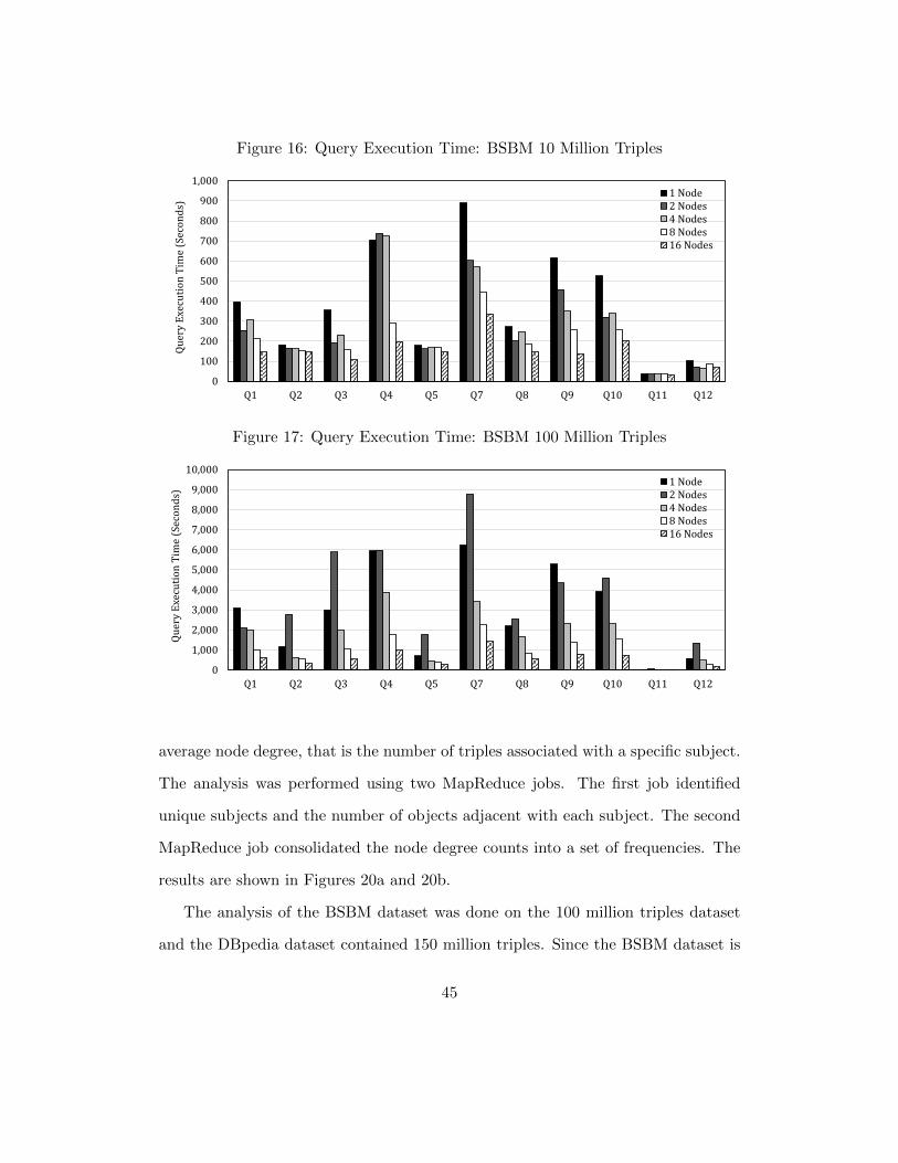
Figure 16: Query Execution Time: BSBM 10 Million Triples

0

100

200

300

400

500

600

700

800

900

1,000

Q1 Q2 Q3 Q4 Q5 Q7 Q8 Q9 Q10 Q11 Q12

Qu

ery

Exe

cuti

on

Tim

e (S

eco

nd

s)

1 Node2 Nodes4 Nodes8 Nodes16 Nodes

Figure 17: Query Execution Time: BSBM 100 Million Triples

0

1,000

2,000

3,000

4,000

5,000

6,000

7,000

8,000

9,000

10,000

Q1 Q2 Q3 Q4 Q5 Q7 Q8 Q9 Q10 Q11 Q12

Qu

ery

Exe

cuti

on

Tim

e (S

eco

nd

s)

1 Node2 Nodes4 Nodes8 Nodes16 Nodes

average node degree, that is the number of triples associated with a specific subject.

The analysis was performed using two MapReduce jobs. The first job identified

unique subjects and the number of objects adjacent with each subject. The second

MapReduce job consolidated the node degree counts into a set of frequencies. The

results are shown in Figures 20a and 20b.

The analysis of the BSBM dataset was done on the 100 million triples dataset

and the DBpedia dataset contained 150 million triples. Since the BSBM dataset is

45

Figure 18: Query Execution Time: BSBM 1 Billion Triples

0

5,000

10,000

15,000

20,000

25,000

30,000

35,000

Q1 Q2 Q3 Q4 Q5 Q7 Q8 Q9 Q10 Q11 Q12

Qu

ery

Exe

cuti

on

Tim

e (S

eco

nd

s)

4 Nodes8 Nodes16 Nodes

Figure 19: Query Execution Time: DBpedia 150 Million Triples

0

100

200

300

400

500

600

700

Q1 Q2 Q3 Q4 Q5 Q6 Q7 Q9 Q10 Q11 Q12 Q13 Q14 Q15 Q16 Q17 Q18 Q19 Q20

Qu

ery

Exe

cuti

on

Tim

e (S

eco

nd

s)

1 Node 2 Nodes 4 Nodes 8 Nodes 16 Nodes

synthetic, both the 10 million and 1 billion triples dataset follow the same frequency

distribution. The number of unique predicates, represented as columns in our table,

is 40 for BSBM and 23,343 for DBpedia. Given these values, we can conclude

that DBpedia contains very sparse data while the BSBM dataset is more densely

populated. Because of this, the DBpedia dataset makes better use of HBase’s null

compression than BSBM.

Given any random subject S∗ from the BSBM dataset, on average, S∗ will

46

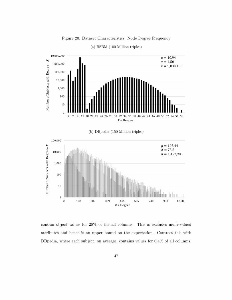
Figure 20: Dataset Characteristics: Node Degree Frequency

(a) BSBM (100 Million triples)

1

10

100

1,000

10,000

100,000

1,000,000

10,000,000

5 7 9 11 18 20 22 24 26 28 30 32 34 36 38 40 42 44 46 48 50 52 54 56 58

Nu

mb

er o

f Su

bje

cts

wit

h D

egre

e =

X

X = Degree

𝜇 = 10.94𝜎 = 4.50𝑛 = 9,034,108

(b) DBpedia (150 Million triples)

1

10

100

1,000

10,000

100,000

2 102 202 309 446 585 740 930 1,468

Nu

mb

er o

f Su

bje

cts

wit

h D

egre

e= X

X = Degree

𝜇 = 105.44𝜎 = 73.8𝑛 = 1,457,983

contain object values for 28% of the all columns. This is excludes multi-valued

attributes and hence is an upper bound on the expectation. Contrast this with

DBpedia, where each subject, on average, contains values for 0.4% of all columns.

47

Table 1: BSBM Query Characteristics [10]

Table 2: Number of Joins Required by BSBM Queries

BSBM Query 1 2 3 4 5 7 8 9 10 11 12

Number of Joins 0 2 0 0 1 4 1 1 1 0 0

We will now examine the query results for each of the datasets.

7.2 Berlin SPARQL Benchmark

As shown in Table 1, the BSBM queries use a diverse set of SPARQL query opera-

tors. These queries generally touch a lot of data with variable subjects. The only

SPARQL and RDF features excluded by this benchmark are named graphs, blank

nodes, collections, REDUCED operator, property hierarchies, and queries in the ASK

form [10].

The slowest BSBM queries are queries 4, 7, and 9. Query 4 uses the UNION

operator. Queries 7 and 9 require 4 and 1 join, respectively. Note that the number

of relations being joined is the number of joins plus one. For the 1 billion triples

dataset, the number of rows with a join key satisfying the join conditions becomes

48

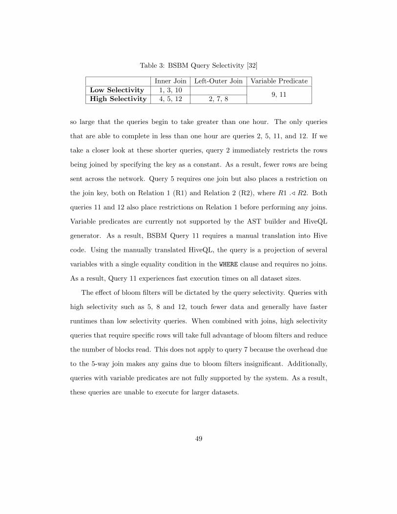
Table 3: BSBM Query Selectivity [32]

Inner Join Left-Outer Join Variable Predicate

Low Selectivity 1, 3, 109, 11

High Selectivity 4, 5, 12 2, 7, 8

so large that the queries begin to take greater than one hour. The only queries

that are able to complete in less than one hour are queries 2, 5, 11, and 12. If we

take a closer look at these shorter queries, query 2 immediately restricts the rows

being joined by specifying the key as a constant. As a result, fewer rows are being

sent across the network. Query 5 requires one join but also places a restriction on

the join key, both on Relation 1 (R1) and Relation 2 (R2), where R1 ./ R2. Both

queries 11 and 12 also place restrictions on Relation 1 before performing any joins.

Variable predicates are currently not supported by the AST builder and HiveQL

generator. As a result, BSBM Query 11 requires a manual translation into Hive

code. Using the manually translated HiveQL, the query is a projection of several

variables with a single equality condition in the WHERE clause and requires no joins.

As a result, Query 11 experiences fast execution times on all dataset sizes.

The effect of bloom filters will be dictated by the query selectivity. Queries with

high selectivity such as 5, 8 and 12, touch fewer data and generally have faster

runtimes than low selectivity queries. When combined with joins, high selectivity

queries that require specific rows will take full advantage of bloom filters and reduce

the number of blocks read. This does not apply to query 7 because the overhead due

to the 5-way join makes any gains due to bloom filters insignificant. Additionally,

queries with variable predicates are not fully supported by the system. As a result,

these queries are unable to execute for larger datasets.

49

7.3 DBpedia SPARQL Benchmark

The DBpedia SPARQL Benchmark introduces simpler queries on a more sparse

dataset. The results presented in Figure 19 indicate faster runtimes for the DBpedia

dataset than the BSBM dataset of similar size (BSBM 100 million in Figure 17).

Looking at Figure 19, we can group queries into two categories: (i) queries that

initially require long runtimes and decrease as the cluster size increases and (ii)

queries that require relatively (fast) constant time for all cluster sizes. The first

group of queries that require long runtimes initially are: 3, 5, 9, 11, 13, 16, 19, and

20. The characteristics of these queries are as follows:

• Queries with string operations on a variable subject or object will require

longer time. This includes language filtering and substring searching.

• Queries with one or more joins require multiple MapReduce jobs and will

require additional time. This includes OPTIONAL clauses which are translated

into left outer joins.

• Queries with variable subjects in the WHERE clause tend to perform more slowly.

Queries that execute in near-constant time for all cluster sizes are reaching a min-

imum query execution time. This can be attributed to the overhead associated

with generating the MapReduce jobs. The variance between runtimes for constant-

time queries can be attributed to various factors including Amazon network usage

spikes or delays due to abnormal behavior of mapper or reducer nodes. Below, we

list characteristics shared by the DBpedia queries that execute between 30 and 60

seconds:

• Subjects are specified and thus we can take full advantage of bloom filters for

fast row access.

50

• Queries generally do not involve variable subjects or objects.

• Unions are not complex (e.g. no joins).

• Queries do not perform string or filter operations. Conditionals such as NOT

NULL execute faster than conditionals involving equalities or inequalities.

Query 17 reports no results since the SPARQL query requires logical operators which

is currently unsupported by our parser.

7.4 Joins

Excluding the size of the dataset, the most important factor in dictating query

execution times is the number of joins. Let |P | denote the number of columns in the

property table, let |S| denote the number of unique subjects and let n denote the

number of joins. In the worst case, an n-way join will require reading (|S||P | ∗ n)

triples from HDFS, sorting these values, and transmitting them across the cluster.

This estimated excludes multivalued attributes. As we can see here, great care must

be taken to eliminate rows that are unlikely to be joined.

7.5 Node Activity

Join selectivity and the number of joins are responsible for the majority of network

traffic in the cluster. In Figure 21, we show data collected during the Berlin SPARQL

Benchmark runs for the master and several slave nodes. All graphs depict metrics

for 1 minute intervals. CPU utilization is averaged over 1 minute and network or

disk is the total bytes moved per minute.

From Figure 21a, we know that all cluster nodes stay beneath 50% CPU uti-

lization. Almost all CPU activity will be for equality comparisons (of joins) or the

51

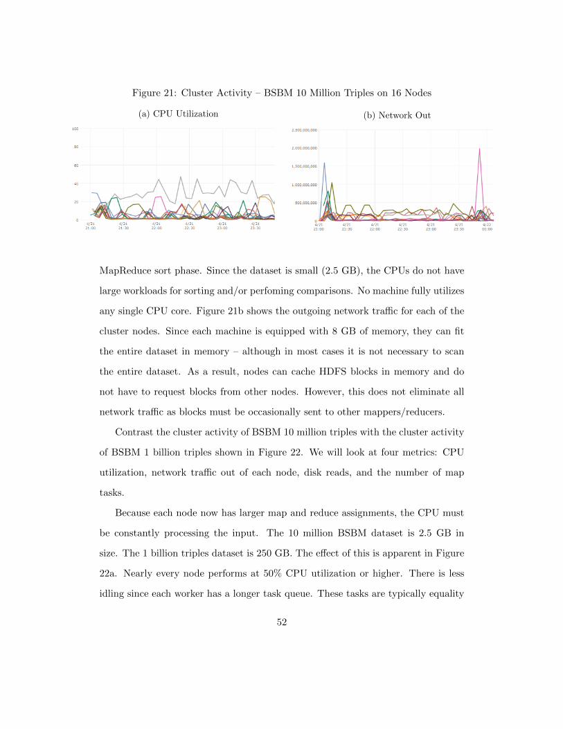
Figure 21: Cluster Activity – BSBM 10 Million Triples on 16 Nodes

(a) CPU Utilization (b) Network Out

MapReduce sort phase. Since the dataset is small (2.5 GB), the CPUs do not have

large workloads for sorting and/or perfoming comparisons. No machine fully utilizes

any single CPU core. Figure 21b shows the outgoing network traffic for each of the

cluster nodes. Since each machine is equipped with 8 GB of memory, they can fit

the entire dataset in memory – although in most cases it is not necessary to scan

the entire dataset. As a result, nodes can cache HDFS blocks in memory and do

not have to request blocks from other nodes. However, this does not eliminate all

network traffic as blocks must be occasionally sent to other mappers/reducers.

Contrast the cluster activity of BSBM 10 million triples with the cluster activity

of BSBM 1 billion triples shown in Figure 22. We will look at four metrics: CPU

utilization, network traffic out of each node, disk reads, and the number of map

tasks.

Because each node now has larger map and reduce assignments, the CPU must

be constantly processing the input. The 10 million BSBM dataset is 2.5 GB in

size. The 1 billion triples dataset is 250 GB. The effect of this is apparent in Figure

22a. Nearly every node performs at 50% CPU utilization or higher. There is less

idling since each worker has a longer task queue. These tasks are typically equality

52

Figure 22: Cluster Activity – BSBM 1 Billion Triples on 16 Nodes

(a) CPU Utilization (b) Network Out

(c) Disk Reads (d) Live Map Tasks

comparisons for the join condition of WHERE clauses or the tasks are sorting the

mapper output.

Moving to Figure 22b, we can see that all cluster nodes move information from

their local disks to other nodes. This is expected due to the nature of HDFS’s

sharding and replication. However, some nodes exhibit network-out rates of 1 GB

or higher for several minutes – sometimes sending data out for over an hour. All data

associated with an RDF subject is typically stored on the same HBase RegionServer.

Depending on the characteristics of the query, if a query references many columns

in a Hive table, the specific RegionServer/slave housing the RDF subject will be

required to send all its data for that subject across network. This results in one

node transmitting more data than other nodes and thus explains the cases of large

53

network out.

The disk reads in Figure 22c are correlated with the network I/O. However,

additional disk reads may be necessary when the relation cannot fit in memory. On

the far right of Figure 22c, most cluster nodes experience 1.5 GB of bytes reads from

disk per minute (about 25 MB/sec). Figure 22d shows us the number of currently

running map tasks. In the left half of the graph, all mappers finished their tasks in

roughly the same time. However, on the right side, most likely attributed to data

skew, some mappers lag behind others.

Summarizing the experiment and analysis – queries with unfiltered joins require

larger amounts of data to be sent across the network resulting in slow query runtimes.

Reducer nodes should be given larger amounts of memory compared to their mapper

counterparts. Mappers must read from disk regardless of the MapReduce step.

However, reducer nodes can place incoming data from the network directly into

memory. Additional memory would be advantageous for reducer nodes. Bloom

filters reduce the number of HDFS blocks read during table scans. As a result,

sparse datasets are able to benefit from this feature and thus enjoy shorter query

runtimes. However, DBpedia also contains simpler benchmark queries.

8 Related Work

Currently a highly debated topic, both classical relational databases and MapReduce

databases both have their advocates and critics. Most enterprises and startups today

are flocking towards distributed database systems due to the era of “big data”.

MapReduce has been proven to scale efficiently, reduce workload execution times,

and enable more powerful analyses.

However, MapReduce is not suitable for all workloads. Several studies have

54

concluded that for datasets less than 1 terabyte (TB), parallel database systems

either perform on par or outperform MapReduce on a cluster of 100 nodes [33, 30].

Several factors affect the performance of MapReduce that do not apply to parallel

databases [25]. Despite these results, several techniques and systems have been

created to solve large-scale data warehousing problems.

Several cloud triple stores exist today and have vast differences among one an-

other. Among these systems are 4store [22], CumulusRDF (Cassandra) [27], HBase

[18], and Couchbase 12. In a comparative study of all of these triple-stores (including

our HBase-Hive implementation), systems using MapReduce introduced significant

query overhead while strictly in-memory stores were unable to accommodate large

datasets [14]. It was discovered that queries involving complex filters generally

performed poorly on NoSQL systems. However, traditional relational database

query optimization techniques work well in NoSQL environments.

It is clear that the increasing amount of data, both structured and unstructured,

will require storage in a distributed manner. Many systems using Google BigTable

variants such as Rya [31], Jena HBase [26], and others [18, 24] are able to efficiently

scale horizontally but often execute queries ranging from seconds to hours. If we are

to migrate future data systems to a distributed environment, several improvements

at the data and query layer are needed.

9 Conclusion

In this thesis, we explored the fundamentals our system’s underlying components

and their intended purpose in our overall database system. We then proceeded to

describe our property table data model and advantages it offers us. The query layer

12http://www.couchbase.com

55

consists of identifying joins given a SPARQL query and generating temporary views

to in an attempt to minimize data transfer during MapReduce.

The results show that sparse datasets make use of many of our property table

design features such as bloom filters and self-join eliminations to improve query

performance. For larger workloads and denser graph datasets, performance becomes

dependent on the join algorithm implementation. SPARQL queries with n-way joins

can take hours to complete.

In the future, we plan to improve upon the naive join algorithms implemented

by our system by investigating alternative parallel join algorithms. We would also

like to provide support for additional SPARQL operators and improve both the AST

and HiveQL optimization. Finally, we would like to explore alternatives to Hadoop

such as distributed shared-memory systems [17].

56

References

[1] Apache hadoop wiki. http://wiki.apache.org/hadoop/.

[2] Apache hbase bulk loading. http://hbase.apache.org/book/arch.bulk.

load.html.

[3] Apache hbase wiki. http://wiki.apache.org/hadoop/Hbase.

[4] Apache hdfs. http://hadoop.apache.org/docs/stable/hdfs_design.html.

[5] The friend of a friend (foaf) project.

[6] Hive hbase integration. https://cwiki.apache.org/confluence/display/

Hive/HBaseIntegration.

[7] Sparql tutorial - optional information. http://jena.apache.org/tutorials/

sparql_optionals.html.

[8] D. J. Abadi, A. Marcus, S. R. Madden, and K. Hollenbach. Scalable semantic

web data management using vertical partitioning. In Proceedings of the

33rd international conference on Very large data bases, pages 411–422. VLDB

Endowment, 2007.

[9] T. Berners-Lee. Linked data design issues. http://www.w3.org/

DesignIssues/LinkedData.html, July 2006.

[10] C. Bizer and A. Schultz. The berlin sparql benchmark. International Journal

on Semantic Web and Information Systems (IJSWIS), 5(2):1–24, 2009.

[11] B. H. Bloom. Space/time trade-offs in hash coding with allowable errors.

Commun. ACM, 13(7):422–426, July 1970.

57

[12] D. Borthakur. The hadoop distributed file system: Architecture and design,

2007.

[13] F. Chang, J. Dean, S. Ghemawat, W. C. Hsieh, D. A. Wallach, M. Burrows,

T. Chandra, A. Fikes, and R. E. Gruber. Bigtable: A distributed storage system

for structured data. ACM Transactions on Computer Systems (TOCS), 26(2):4,

2008.

[14] P. Cudre-Mauroux, I. Enchev, S. Fundatureanu, P. Groth, A. Haque, A. Harth,

F. L. Keppmann, D. Miranker, J. Sequeda, and M. Wylot. Nosql databases

for rdf: An empirical evaluation. In The Semantic Web – ISWC 2013, volume

8219 of Lecture Notes in Computer Science, pages 310–325. Springer Berlin

Heidelberg, 2013.

[15] J. Dean and S. Ghemawat. Mapreduce: simplified data processing on large

clusters. Communications of the ACM, 51(1):107–113, 2008.

[16] L. Ding and T. Finin. Characterizing the semantic web on the web. In The 5th

International Semantic Web Conference, ISWC 2006, pages 242–257. Springer,

2006.

[17] C. Engle, A. Lupher, R. Xin, M. Zaharia, M. J. Franklin, S. Shenker,

and I. Stoica. Shark: fast data analysis using coarse-grained distributed

memory. In Proceedings of the 2012 ACM SIGMOD International Conference

on Management of Data, pages 689–692. ACM, 2012.

[18] S. Fundatureanu. A Scalable RDF Store Based on HBase. Master’s thesis, VU

University Amsterdam, Sept. 2012.

58

[19] M. A. Gallego, J. D. Fernandez, M. A. Martınez-Prieto, and P. de la Fuente. An

empirical study of real-world sparql queries. In 1st International Workshop on

Usage Analysis and the Web of Data (USEWOD2011) at the 20th International

World Wide Web Conference (WWW 2011), Hydebarabad, India, 2011.

[20] L. George. HBase: the definitive guide. O’Reilly, 2011.

[21] S. Ghemawat, H. Gobioff, and S.-T. Leung. The google file system. In

Proceedings of the nineteenth ACM symposium on Operating systems principles,

SOSP ’03, pages 29–43, New York, NY, USA, 2003. ACM.

[22] S. Harris, N. Lamb, and N. Shadbolt. 4store: The design and implementation

of a clustered rdf store. In 5th International Workshop on Scalable Semantic

Web Knowledge Base Systems (SSWS2009), pages 94–109, 2009.

[23] M. Hausenblas, W. Halb, Y. Raimond, and T. Heath. What is the size of the

semantic web. Proceedings of I-Semantics, pages 9–16, 2008.

[24] M. F. Husain, P. Doshi, L. Khan, and B. Thuraisingham. Storage and retrieval

of large rdf graph using hadoop and mapreduce. In Cloud Computing, pages

680–686. Springer, 2009.

[25] D. Jiang, B. C. Ooi, L. Shi, and S. Wu. The performance of mapreduce: an

in-depth study. Proc. VLDB Endow., 3(1-2):472–483, Sept. 2010.

[26] V. Khadilkar, M. Kantarcioglu, B. M. Thuraisingham, and P. Castagna. Jena-

hbase: A distributed, scalable and effcient rdf triple store. In International

Semantic Web Conference (Posters & Demos), 2012.

59

[27] G. Ladwig and A. Harth. Cumulusrdf: Linked data management on nested

key-value stores. In The 7th International Workshop on Scalable Semantic

Web Knowledge Base Systems (SSWS 2011), page 30, 2011.

[28] M. Morsey, J. Lehmann, S. Auer, and A.-C. N. Ngomo. Dbpedia sparql

benchmark–performance assessment with real queries on real data. In The

Semantic Web–ISWC 2011, pages 454–469. Springer, 2011.

[29] O. OMalley. Terabyte sort on apache hadoop. Yahoo, available online at:

http://sortbenchmark. org/Yahoo-Hadoop. pdf,(May), pages 1–3, 2008.

[30] A. Pavlo, E. Paulson, A. Rasin, D. J. Abadi, D. J. DeWitt, S. Madden, and

M. Stonebraker. A comparison of approaches to large-scale data analysis. In

Proceedings of the 2009 ACM SIGMOD International Conference on Manage-

ment of data, SIGMOD ’09, pages 165–178, New York, NY, USA, 2009. ACM.

[31] R. Punnoose, A. Crainiceanu, and D. Rapp. Rya: a scalable rdf triple store

for the clouds. In Proceedings of the 1st International Workshop on Cloud

Intelligence, page 4. ACM, 2012.

[32] J. F. Sequeda and D. P. Miranker. Ultrawrap: Sparql execution on relational

data. Technical report, Technical Report TR-12-10, University of Texas at

Austin, Department of Computer Sciences, 2012.

[33] M. Stonebraker, D. Abadi, D. J. DeWitt, S. Madden, E. Paulson, A. Pavlo, and

A. Rasin. Mapreduce and parallel dbmss: friends or foes? ACM, 53(1):64–71,

Jan. 2010.

[34] L. Tang and N. Jain. Join strategies in hive. Yahoo! Hive Summit, 2011.

60

[35] A. Thusoo, J. S. Sarma, N. Jain, Z. Shao, P. Chakka, S. Anthony, H. Liu,

P. Wyckoff, and R. Murthy. Hive: a warehousing solution over a map-reduce

framework. Proceedings of the VLDB Endowment, 2(2):1626–1629, 2009.

[36] C. Weiss, P. Karras, and A. Bernstein. Hexastore: sextuple indexing for

semantic web data management. Proceedings of the VLDB Endowment,

1(1):1008–1019, 2008.

[37] T. White. Hadoop: the definitive guide. O’Reilly, 2012.

[38] K. Wilkinson and K. Wilkinson. Jena property table implementation, 2006.

[39] S. Wu, F. Li, S. Mehrotra, and B. C. Ooi. Query optimization for massively

parallel data processing. In Proceedings of the 2nd ACM Symposium on Cloud

Computing, SOCC ’11, pages 12:1–12:13, New York, NY, USA, 2011. ACM.

61

A Reproducing the Evaluation Environment

A.1 Amazon Elastic MapReduce

To set up the EC2 cluster with Hadoop, HBase, and Hive, use the instructions below

and on the project’s website13. These instructions were made using the EC2 portal

as of December 2013.

1. Navigate to the AWS Management Console and go to the Elastic MapReduceservice.

2. Click Create Cluster.

3. Under Software Configuration, select the appropriate version of Hadoop.

4. If HBase is not listed under Applications to be installed, add it and ignore thebackup steps.

5. If Hive is not listed under Applications to be installed, add it and select theappropriate Hive version.

6. All instance types should be m1.large by default.

7. Under Hardware Configuration, in the Core instance type, enter the numberof slave nodes for the cluster (1, 2, 4, 8, or 16 used in this experiment).

8. Task Instance Group should be zero.

9. Select your EC2 key pair and leave all other options to default.

10. Under Bootstrap Actions, add a new, Custom action.

11. For the S3 Location enter:s3://us-east-1.elasticmapreduce/bootstrap-actions/configure-hbase.

12. For Optional Arguments enter:-s hbase.hregion.max.filesize=10737418240.

13. Add the bootstrap action.

14. Review your settings and click Create Cluster.

15. The cluster will take 3-5 minutes to fully initialize.

13https://github.com/ahaque/hive-hbase-rdf/

62

A.2 HBase Parameter Settings

Table 4 lists specific parameters and values that were changed in HBase. Many of

these settings can be configured in HBase’s configuration files or by using the Java

API when creating the table.

Table 4: Custom HBase Parameters

Parameter Name Value

HBase Table

hbase.hregion.max.filesize 10737418240hbase.hstore.blockingStoreFiles 25hbase.hregion.memstore.block.multiplier 8hbase.regionserver.handler.count 30hbase.regions.percheckin 30hbase.regionserver.global.memstore.upperLimit 0.3hbase.regionserver.global.memstore.lowerLimit 0.15

Column Family

HColumnDescriptor.BloomFilterType rowcolHColumnDescriptor.Cache Blooms On Write trueHColumnDescriptor.MaxVersions 100

63

B Detailed Evaluation Tables

The value NaN denotes the query encountered an error and was aborted or was

interrupted due to long runtime.

B.1 Query Execution Time

Table 5: BSBM 10 Million Triples (Geometric Average in Seconds)

1 Node 2 Nodes 4 Nodes 8 Nodes 16 Nodes

Q1 395.82 254.49 307.9 215.35 146.35

Q2 181.91 165.32 160.97 150.87 144.49

Q3 354.55 192.83 231.96 156.26 106.05

Q4 705.96 737.82 725.21 292.48 196.56

Q5 178.55 161.36 168.21 167.29 147.78

Q7 889.83 602.84 569.87 446.54 335.63

Q8 271.94 202.84 247.64 184.74 146.29

Q9 615.42 457.34 349.46 259.7 137.27

Q10 526.03 319.47 339.01 258.55 203.17

Q11 36.64 36.3 36.24 36.52 33.58

Q12 102.55 72.25 66.01 85.13 68.13

Table 6: BSBM 100 Million Triples (Geometric Average in Seconds)

1 Node 2 Nodes 4 Nodes 8 Nodes 16 Nodes

Q1 3085.51 2108.00 2015.53 1003.02 615.66

Q2 1161.68 2772.77 626.99 569.72 348.65

Q3 3007.65 5883.78 2014.42 1039.08 544.22

Q4 5954 5985.29 3888.06 1775.04 1005.08

Q5 703.21 1771.99 466.63 402.10 270.69

Q7 6233.79 8774.58 3400.93 2286.69 1417.31

Q8 2195.31 2559.48 1679.84 813.22 569.76

Q9 5278.52 4349.19 2321.37 1403.70 805.56

Q10 3914.52 4603.91 2311.9 1564.91 749.63

Q11 36.30 50.60 35.94 35.11 35.45

Q12 582.66 1352.29 484.57 300.05 174.24

64

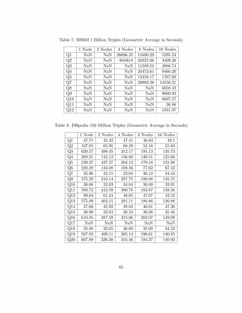
Table 7: BSBM 1 Billion Triples (Geometric Average in Seconds)

1 Node 2 Nodes 4 Nodes 8 Nodes 16 Nodes

Q1 NaN NaN 26696.25 11690.29 5295.24

Q2 NaN NaN 40100.8 20337.06 3409.26

Q3 NaN NaN NaN 11289.52 4986.74

Q4 NaN NaN NaN 20473.61 9460.20

Q5 NaN NaN NaN 12458.17 1767.69

Q7 NaN NaN NaN 29989.26 14556.21

Q8 NaN NaN NaN NaN 6058.42

Q9 NaN NaN NaN NaN 9060.93

Q10 NaN NaN NaN NaN 9007.57

Q11 NaN NaN NaN NaN 36.86

Q12 NaN NaN NaN NaN 1851.97

Table 8: DBpedia 150 Million Triples (Geometric Average in Seconds)

1 Node 2 Nodes 4 Nodes 8 Nodes 16 Nodes

Q1 47.71 45.32 47.41 46.83 49.1

Q2 107.05 65.95 68.29 53.16 55.93

Q3 620.57 498.45 312.17 195.13 135.73

Q4 208.51 142.12 136.69 130.51 125.60

Q5 539.37 437.27 264.13 179.18 131.98

Q6 220.29 133.08 108.56 77.02 67.42

Q7 35.96 33.15 33.64 36.12 34.44

Q9 575.29 310.14 297.75 190.08 145.75

Q10 36.68 32.03 34.04 36.00 33.91

Q11 580.72 412.59 300.78 183.67 138.56

Q12 99.04 61.24 48.05 47.07 42.52

Q13 575.09 402.15 291.11 186.86 120.88

Q14 47.66 45.92 48.03 46.61 47.36

Q15 36.90 32.04 36.53 36.06 35.46

Q16 610.85 387.59 315.06 202.07 149.09

Q17 NaN NaN NaN NaN NaN

Q18 35.88 32.05 36.69 35.00 34.23

Q19 597.83 499.11 305.14 196.61 140.85

Q20 607.89 336.38 316.46 194.37 140.92

65

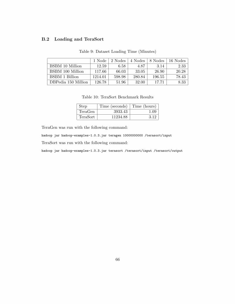
B.2 Loading and TeraSort

Table 9: Dataset Loading Time (Minutes)

1 Node 2 Nodes 4 Nodes 8 Nodes 16 Nodes

BSBM 10 Million 12.59 6.58 4.87 3.14 2.33

BSBM 100 Million 117.66 66.03 33.05 26.90 20.28

BSBM 1 Billion 1214.01 598.98 280.84 196.55 78.43

DBPedia 150 Million 126.78 51.96 32.00 17.71 8.33

Table 10: TeraSort Benchmark Results

Step Time (seconds) Time (hours)

TeraGen 3933.43 1.09

TeraSort 11234.88 3.12

TeraGen was run with the following command:

hadoop jar hadoop-examples-1.0.3.jar teragen 10000000000 /terasort/input

TeraSort was run with the following command:

hadoop jar hadoop-examples-1.0.3.jar terasort /terasort/input /terasort/output

66

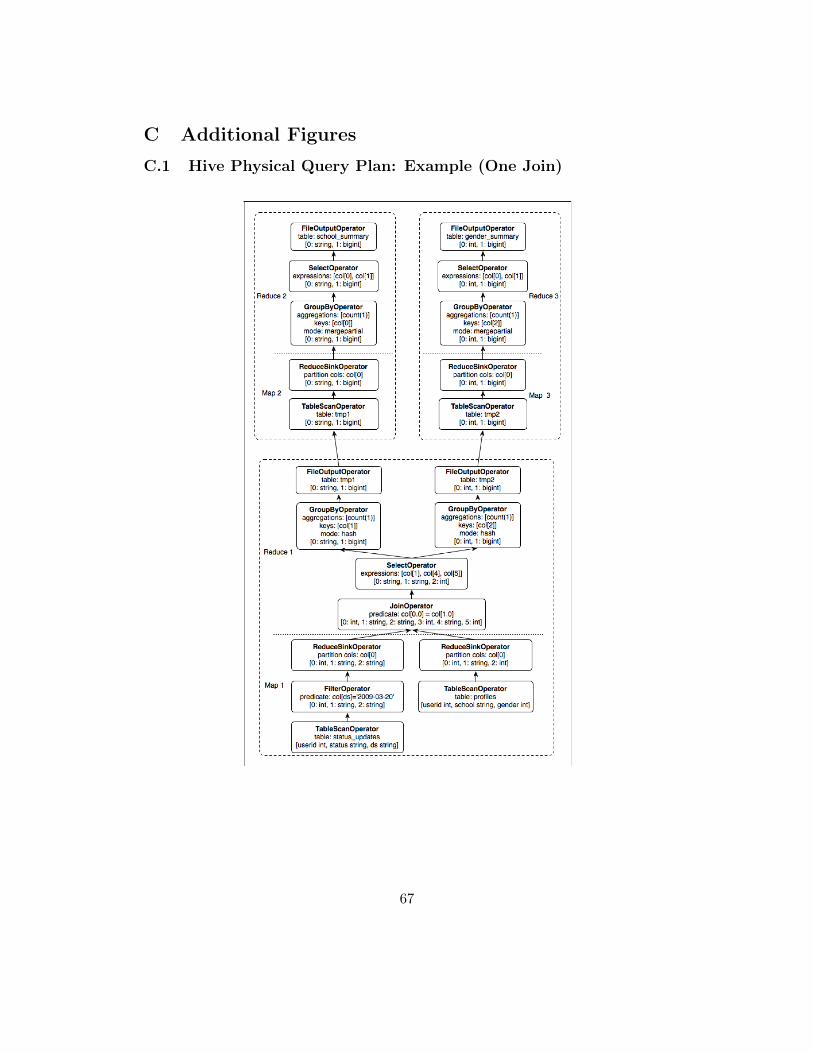
C Additional Figures

C.1 Hive Physical Query Plan: Example (One Join)

67

C.2 Hive Physical Query Plan: BSBM Query 1 (No Joins)

STAGE DEPENDENCIES:

Stage-1 is a root stage

Stage-2 depends on stages: Stage-1

Stage-0 is a root stage

STAGE PLANS:

Stage: Stage-1

Map Reduce

Alias -> Map Operator Tree:

TableScan

alias: rdf1

Filter Operator

Select Operator

expressions:

expr: key

type: string

expr: rdfs_label

type: string

outputColumnNames: key, rdfs_label

Group By Operator

bucketGroup: false

Reduce Output Operator

sort order: ++

Reduce Operator Tree:

Group By Operator

Select Operator

expressions:

expr: _col0

type: string

expr: _col1

type: string

outputColumnNames: _col0, _col1

File Output Operator

Stage: Stage-2

Map Reduce

Alias -> Map Operator Tree:

Reduce Output Operator

key expressions:

expr: _col1

type: string

sort order: +

Reduce Operator Tree:

Extract

Limit

File Output Operator

Stage: Stage-0

Fetch Operator

limit: 10

68

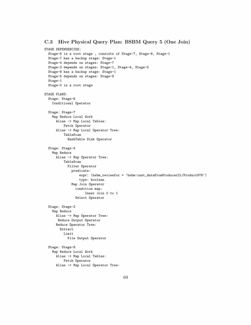
C.3 Hive Physical Query Plan: BSBM Query 5 (One Join)

STAGE DEPENDENCIES:

Stage-6 is a root stage , consists of Stage-7, Stage-8, Stage-1

Stage-7 has a backup stage: Stage-1

Stage-4 depends on stages: Stage-7

Stage-2 depends on stages: Stage-1, Stage-4, Stage-5

Stage-8 has a backup stage: Stage-1

Stage-5 depends on stages: Stage-8

Stage-1

Stage-0 is a root stage

STAGE PLANS:

Stage: Stage-6

Conditional Operator

Stage: Stage-7

Map Reduce Local Work

Alias -> Map Local Tables:

Fetch Operator

Alias -> Map Local Operator Tree:

TableScan

HashTable Sink Operator

Stage: Stage-4

Map Reduce

Alias -> Map Operator Tree:

TableScan

Filter Operator

predicate:

expr: (bsbm_reviewfor = ’bsbm-inst_dataFromProducer21/Product978’)

type: boolean

Map Join Operator

condition map:

Inner Join 0 to 1

Select Operator

Stage: Stage-2

Map Reduce

Alias -> Map Operator Tree:

Reduce Output Operator

Reduce Operator Tree:

Extract

Limit

File Output Operator

Stage: Stage-8

Map Reduce Local Work

Alias -> Map Local Tables:

Fetch Operator

Alias -> Map Local Operator Tree:

69

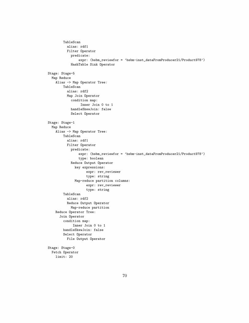
TableScan

alias: rdf1

Filter Operator

predicate:

expr: (bsbm_reviewfor = ’bsbm-inst_dataFromProducer21/Product978’)

HashTable Sink Operator

Stage: Stage-5

Map Reduce

Alias -> Map Operator Tree:

TableScan

alias: rdf2

Map Join Operator

condition map:

Inner Join 0 to 1

handleSkewJoin: false

Select Operator

Stage: Stage-1

Map Reduce

Alias -> Map Operator Tree:

TableScan

alias: rdf1

Filter Operator

predicate:

expr: (bsbm_reviewfor = ’bsbm-inst_dataFromProducer21/Product978’)

type: boolean

Reduce Output Operator

key expressions:

expr: rev_reviewer

type: string

Map-reduce partition columns:

expr: rev_reviewer

type: string

TableScan

alias: rdf2

Reduce Output Operator

Map-reduce partition

Reduce Operator Tree:

Join Operator

condition map:

Inner Join 0 to 1

handleSkewJoin: false

Select Operator

File Output Operator

Stage: Stage-0

Fetch Operator

limit: 20

70