copyright © 2015 by academic publishing house...

Modeling of Artificial Intelligence, 2015, Vol.(6), Is. 2

137

Copyright © 2015 by Academic Publishing House Researcher

Published in the Russian Federation Modeling of Artificial Intelligence Has been issued since 2014. ISSN: 2312-0355

Vol. 6, Is. 2, pp. 137-149, 2015 DOI: 10.13187/mai.2015.6.137 www.ejournal11.com

UDC 004

Effects of Technical Market Indicators

on Stock Market Index Direction Forecasting

1 Günter Şenyurt 2 Abdülhamit Subaşı

1 International Burch University, Bosnia and Herzegovina Francuske revolucije bb, Ilidza 71210 M. Sc. (Information Technologies), Assistant Lecturer E-mail: [email protected] 2 International Burch University, Bosnia and Herzegovina Francuske revolucije bb, Ilidza 71210 Doctor (Electrical Eng.), Professor E-mail: [email protected]

Abstract In this study, we examine and compare the performances of data mining techniques based on

the daily indexes of five different markets, namely DAX, FTSE 100, NASDAQ Composite, NIKKEI 225 and NYSE Composite. The A/D oscillator, chaikin oscillator, moving average convergence/divergence, stochastic oscillator, acceleration, momentum, chaikin volatility, fast stochastics, slow stochastics, williams %R, negative volume index, positive volume index, relative strength index, accumulation/distribution line, bollinger band, highest high, lowest low, median price, on balance volume, price rate of change, price-volume trend, typical price, volume rate of change, weighted close and williams accumulation/distribution make up the 28 technical indicator attributes used in this study. The data mining techniques utilized in this study comprise of random forest model, artificial neural network (ANN) and support vector machine (SVM). Initially, the input features are sorted with WEKA’s Info Ranker which reveals the best attributes based on relative weight. Afterwards, ten attributes having the highest relative weight values are fed into random forest, ANN and SVM. Then different attribute combinations based on their relative weights are tested in turns for more precision.

Keywords: market movement direction, SVM, ANN, RF, forecasting, data mining techniques, technical market indicators.

Introduction and Literature Review The prediction of market index price movement direction is one of the most intriguing

problems in the financial sphere. Even those who professionalize in adding value to invested assets or try minimizing the risks involved could not find a single answer to the market direction question. Will it see a rise tomorrow or will it face a decline? In the last couple of decades, investors and researchers alike are trying to find robust forecasting methods in order to make accurate market decisions. They are on the unending lookout for a trustworthy method to predict stock market trends. It is the nonlinearity or in other words the non-stationary aspect of the markets that

http://www.ejournal11.com/


138

makes life difficult for people who are trying to understand the market behavior on a reliable basis. Habitually the fundamental approach to estimate the outcome of a financial time series is a number of statistical methods such as GARCH, ARMA and ARIMA, which have been used around for some time but inherently suffer from the postulation of linear variability of the stock price indexes during a particular period of time.

Particularly, the statistical method does not produce an automated solution, since at each step it necessitates changes and adaptations in order to meet regularity and stationarity in the target value. Hence, in order to trace the complex and non-stationary character of the markets more powerful methods are required to eliminate the shortcomings of the customary statistical approaches. Thus, professionals of the financial world have come up with several new ways to make sound trading decisions. Some of these astute computational methods include artificial neural networks (ANN), support vector machines (SVM) and fuzzy logic systems [1]. ANNs variants include the radial basis function neural network RBFNN [2], recurrent neural network RNN [3], multilayer perceptron MLP [4], generalized regression neural networks GRNN [5], random vector functional link neural network FLANN [6], local linear wavelet neural network LLWNN [7] and wavelet neural network WNN [8]. These neural network designs, nonetheless, cannot show strong performance owing to the volatile and multidimensional character of the dataset coupled which is coupled with noise, as well. In this sense, computations based on fuzzy logic are preferred by some analysts due to its high handling capacity of data uncertainties. Fusion techniques have been proposed like the consolidation of neural networks with fuzzy systems [1]. Some constructs may well include fuzzy neural networks FNN [9], adaptive network fuzzy information system ANFIS [10] or wavelet fuzzy neural networks WLFNN [11]. Neural networks can be enhanced through certain methods such as the genetic algorithm, particle swarm optimization [12] or bacterial foraging optimization [13] so that in order to boost the accuracy of forecasting the best set of parameters can be gained. A three featured neural network prediction apparatus is the main subject of [14]. Moreover, the associated performance of this model to other settled prediction mechanisms is examined and portrayed by several empirical works. Considering the real Chinese financial market in 2007, the direction of fluctuations and the investment atmosphere at the time may be taken as exemplary to the shift of market behavior. Consequently, a time-variant historical dataset that comes part of a training set is able to mirror the possible market conduct motives. When the whole data is used to train the network in an equal manner, the network composition may not be persistent with the authentic stock market dynamism. Expressly, in the present Chinese stock exchanges, rules of transactions and management structures are promptly transforming, thus it is hard to follow up on the developments in the markets since the historical data cannot live up to the point of representing the current situation. Nevertheless, when the latest data is chosen, lots of precious information gets lost that the antecedent data grips. [15] suggests a propitious solution founded on Legendre neural network where weight sums are fed into the input and the orthogonal function is used as the hidden layer transfer function to overcome this issue. In their study, market indexes like Dow Jones and NASDAQ Composite is tested to see the forecasting strength of their LNNRT mechanism. In financial forecasting, two suppositions come forward when predicting market indexes. One is the Efficient Market Hypothesis assuming that market prices contain all the necessary information already shared by market players about the market price outcome. Since all the information is presumably there to exploit the market, price changes must happen in a random style due to the fact that new information comes in randomly. Thus, the term ―random walk‖ was coined and meant to address the impossibility to predict the market price outcome or in other words there are no trends or patterns to describe the market behavior. Accordingly, price variations happen as a consequence of information delays or data incompleteness. Even though peripheral incidents can impact stock market price levels, precise forecasting never works due to the hardship of modeling such outside factors.

Putting aside the ample debate whether the Efficient Market Hypothesis is true or not, the onset of smart finance has opened way to another hypothesis that is based on the idea of a not always efficient market mechanism which is ridden with incapability. In other words, the market price can actually be predicted in some way owing to certain inefficiencies [16]. That many market players have beaten the market unfailingly, using smart computations, could be a manifestation that the Efficient Market Hypothesis might not be necessarily correct, at least in practice [17]. The market price forecasting profession and the affiliated decision system supporting plays a


139

crucial role in today’s smart finance environment. For a long while, researchers have been conducting extensive studies to understand the underlying mechanism of stock markets and to accurately predict the market price outcome. Since money business is all about garnering high financial gains, every player in the market is after some smart mathematical scheme that would be able to pick winners and write off losers in a consistent manner. Daily market values constitute a string of numbers over time capturing information that needs to be processed by computational models. Classical models such as moving average, ARIMA or exponential smoothing schemes suggest linear relationships between the market attributes in future value forecasting [18-25].

User specified model functions may take a long time to evolve by experimenting with disparate probable relations and algorithms. Though linear models are appreciated and credited to some certain extent, scientific research indicates that stock markets are highly chaotic systems that cannot be deciphered by linear function relationships. Due to irregularities in a chaos system it may look random but in reality relations are nonlinear and deterministic in nature. Accordingly, in finance complex nonlinear time series models are more realistic than linear models, though not inconsistent with linear solutions that can be used by specialists. While linear systems may be seen as rough estimations of nonlinear relations in forecasting, it is not fortuitous that neural networks or genetic algorithms attract a lot of scrutiny among researchers [26-27]. The term ―random walk‖ implies that historical data is already reserved in the current market value, whereas, all increments both negative or positive negate each other over a certain time span resulting in balance of an expected value equal to zero due to the fact that they are not correlated. The seemingly hard to predict random walk model needs a nonlinear model supplement that can efficiently forecast the market addressing the several intrinsic factors that are so far not totally conceived. The difference with smart systems is that they can analyze and test historical data to infer future predictions. The power of intelligent computation schemes is that they do not have many postulations of the hidden functional dependencies and their incipient conditions, since markets may not be truly efficient systems as customary financial theory puts it [17].

While the use of artificial intelligence in finance is not new, the biggest boost ever in AI has been done in problem solving; new ideas and approaches for designing better schemes that concentrate on problems rather than calculations. Several works have collated the efficiency of artificial intelligence techniques over traditional models such as ARMA, ARIMA, linear regression et cetera in forecasting questions that revealed the superior estimation quality of artificial intelligence based schemes, [28-30]. Recently, numerous works have focused either on artificial intelligent systems or their combinations with other models to increase the precision of forecasting [31]. [28-29] suggests an integrated system founded by genetic fuzzy model and artificial neural network as a stock price estimation expert system. To sort out the dominant factors of the stock prices they made use of stepwise regression analysis, then partitioned the unprocessed data into clusters by the use of self-organizing map. In the last step, these clusters are presented to the genetic fuzzy system which can sunder out the rule bases and tune the data base. Their outcomes proved better performance than other approaches. A Takagi-Sugeno-Kang type fuzzy rule based system made use of simulated annealing to train the most impacting parameters. The outcome revealed better performance of this fuzzy model over back propagation network or alike [32]. [33] tested the Tehran Stock Exchange by a neuro-fuzzy inference system where C-mean clustering was applied. The model proved promising over similar solutions. [34] brings out his swarm algorithm that serves the purpose of optimizing a K-means clustering algorithm in the learning course of the radial basis function. They tested their proposed approach against two other optimization methods as well as some well-known forecasting methods only to see its better performance.

[35] have a solution to the problem of non-differentiability of morphological operators in their proposition of dilation-erosion perceptron used with the back propagation algorithm. [36]’s investment apparatus is remarkable as for it is designed to construct forecasting models for investors. [37] wanted to find a way to find buy or sell indications derived from technical indicators fed into a classifier based on a genetic algorithm. The classifier worked well demonstrating powerful forecasting capability. Neural networks are powerful mechanisms that can overcome the complexity of input and output associations. Inspired by the human brain, they are designed to learn from experience; handling data, saving essential attributes of the input and postulating from past experience [38].


140

Most literature on artificial neural networks concentrates on back-propagation that is found to be converging poorly. Derivatives of the back-propagation algorithm puts emphasis on the better training and converging aspect such as the Levenberg-Marquardt back propagation [39]. Nonetheless, two fundamental issues with Levenberg-Marquardt back propagation has led researchers to use evolutionary algorithms in order to obtain more proper network weights [40-41]. Evolutionary models such as genetic algorithms have helped researchers a great deal to make up for the deficiencies in back-propagation networks like finding global minima in intricate spaces or permitting the fitness assessment to consider ancillary factors in the back-propagation algorithm [42]. It is also found that genetic algorithms perform stronger than back-propagation networks [43-45].

A rather different concept called nonlinear filtering has been intensively used in signal processing applications. One noteworthy branch of nonlinear systems is founded on the scheme of mathematical morphology [46]. A decent amount of research has been made on the morphological system architecture [47-49]. The embedding of filters into artificial neural networks using morphological rank linear agents at each processing node is the theme of [50].

Asia, a major player in the global financial circles with its better growth rates, expanding economies backed by a large consumer base strike the interest of many researchers [51-53]. Japan and China are examples of two different stock markets. Japan is a showcase of a mature financial market with lots of research being conducted on [54-58]. On the other hand, China is an archetypical model of a young emerging stock market with fewer studies conducted on [54] and [59]. Quite a bit of efficacious applications has revealed that neural networks are a promising technique to predict stock prices and indexes. The nonlinear mapping function of neural networks does not require a presupposition of the data properties [54, 59-61]. In order to construct a forecasting model with neural networks, the original observed data is used exactly [60-61]. The price levels of stocks are influenced by many intrinsic factors such as economic affairs, seasonality or other factors [62-66]. For instance, the stock market reacts to a couple of factors like news from companies, political problems, government related issues, psychological influences etc. [66]. [62] wielded Independent component analysis for the largest Japanese stocks’ daily return correction. According to the results dominant Independent components disclosed more intrinsic information of the stock price levels than principal component analysis [67].

Independent components are the so-called independent sources (ICs) that represent the concealed information of the clear data. Two types of the independent component analysis models are the linear and the nonlinear independent component analysis models. The linear model assumes the observable data is formed by a linear mixture of independent components, whereas, the nonlinear model hypothesizes that the observations consist of nonlinear blending of independent components [67-70]. [71] put to use LICA as an attribute selection apparatus to establish a support vector machine predictor. The independent components were regarded as attributes of the prediction data and engaged to construct the support vector machine standard. [58] asserted a two-phase prediction apparatus by coalescing LICA and support vector regression in financial time series forecasting. LICA was initially employed to the predicting parameters for the inducing ICs. After pinpointing and clearing away the ICs holding noise, the remaining ICs were then utilized to rebuild the predicting parameters enclosing less noise and held the role as the input parameters of the SVR prediction standard.

[57] used LICA to induce a de-noising design for data of stock prices. The design was then utilized as a pre-mechanism device before constructing a forecasting apparatus for stock prices.

Linear ICA is convenient to use when it makes sense to presume that the mixing instrument is linear or the observed data is a linear mixture. However, in several pragmatic cases or problems, the observations (for instance, stock index data) could be a nonlinear blend of concealed source signals. Stock markets in Asia, for example, are extremely active and able to display broad changes because a lot of global investors are allured towards Asian stock markets. This in fact, may practically cause Asian stock market indexes to become nonlinear sets of data where NLICA has a huge potential as a forecasting apparatus [72-73, 68].


141

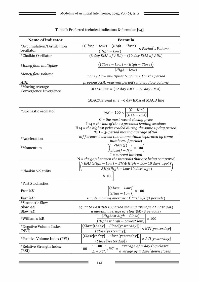
Table I: Preferred technical indicators & formulae [74]

Name of indicator Formula

*Accumulation/Distribution oscillator

𝐶𝑙𝑜𝑠𝑒 − 𝐿𝑜𝑤 − 𝐻𝑖𝑔𝑕 − 𝐶𝑙𝑜𝑠𝑒

𝐻𝑖𝑔𝑕 − 𝐿𝑜𝑤 × 𝑃𝑒𝑟𝑖𝑜𝑑′𝑠 𝑉𝑜𝑙𝑢𝑚𝑒

*Chaikin Oscillator

3 𝑑𝑎𝑦 𝐸𝑀𝐴 𝑜𝑓 𝐴𝐷𝐿 − 10 𝑑𝑎𝑦 𝐸𝑀𝐴 𝑜𝑓 𝐴𝐷𝐿

Money flow multiplier

𝐶𝑙𝑜𝑠𝑒 − 𝐿𝑜𝑤 − 𝐻𝑖𝑔𝑕 − 𝐶𝑙𝑜𝑠𝑒

𝐻𝑖𝑔𝑕 − 𝐿𝑜𝑤

Money flow volume

𝑚𝑜𝑛𝑒𝑦 𝑓𝑙𝑜𝑤 𝑚𝑢𝑙𝑡𝑖𝑝𝑙𝑖𝑒𝑟 × 𝑣𝑜𝑙𝑢𝑚𝑒 𝑓𝑜𝑟 𝑡𝑕𝑒 𝑝𝑒𝑟𝑖𝑜𝑑

ADL previous ADL +current period’s money flow volume *Moving Average Convergence Divergence

𝑀𝐴𝐶𝐷 𝑙𝑖𝑛𝑒 = 12 𝑑𝑎𝑦 𝐸𝑀𝐴 − 26 𝑑𝑎𝑦 𝐸𝑀𝐴

(MACD)𝑆𝑖𝑔𝑛𝑎𝑙 𝑙𝑖𝑛𝑒 =9 day EMA of MACD line

*Stochastic oscillator

%𝐾 = 100 × 𝐶 − 𝐿14

𝐻14 − 𝐿14

C = the most recent closing price L14 = the low of the 14 previous trading sessions

H14 = the highest price traded during the same 14 day period %D = 3- period moving average of %K

*Acceleration 𝑑𝑖𝑓𝑓𝑒𝑟𝑒𝑛𝑐𝑒 𝑏𝑒𝑡𝑤𝑒𝑒𝑛 two momentums separated by some

numbers of periods

*Momentum 𝑐𝑙𝑜𝑠𝑒(𝐽)

𝑐𝑙𝑜𝑠𝑒(𝐽 − 𝑁) × 100

J = current interval

N = the gap between the intervals that are being compared

*Chaikin Volatility

𝐸𝑀𝐴 𝐻𝑖𝑔𝑕 − 𝐿𝑜𝑤 − 𝐸𝑀𝐴(𝐻𝑖𝑔𝑕 − 𝐿𝑜𝑤 10 𝑑𝑎𝑦𝑠 𝑎𝑔𝑜)

𝐸𝑀𝐴(𝐻𝑖𝑔𝑕 − 𝐿𝑜𝑤 10 𝑑𝑎𝑦𝑠 𝑎𝑔𝑜)

× 100

*Fast Stochastics

Fast %K 𝐶𝑙𝑜𝑠𝑒 − 𝐿𝑜𝑤

𝐻𝑖𝑔𝑕 − 𝐿𝑜𝑤 × 100

Fast %D 𝑠𝑖𝑚𝑝𝑙𝑒 𝑚𝑜𝑣𝑖𝑛𝑔 𝑎𝑣𝑒𝑟𝑎𝑔𝑒 𝑜𝑓 𝐹𝑎𝑠𝑡 %𝐾 (3 𝑝𝑒𝑟𝑖𝑜𝑑𝑠)

*Stochastic Slow Slow %K 𝑒𝑞𝑢𝑎𝑙 𝑡𝑜 𝐹𝑎𝑠𝑡 %𝐷 (3 𝑝𝑒𝑟𝑖𝑜𝑑 𝑚𝑜𝑣𝑖𝑛𝑔 𝑎𝑣𝑒𝑟𝑎𝑔𝑒 𝑜𝑓 𝐹𝑎𝑠𝑡 %𝐾) Slow %D 𝑎 𝑚𝑜𝑣𝑖𝑛𝑔 𝑎𝑣𝑒𝑟𝑎𝑔𝑒 𝑜𝑓 𝑠𝑙𝑜𝑤 %𝐾 (3 𝑝𝑒𝑟𝑖𝑜𝑑𝑠)

*William’s %R 𝐻𝑖𝑔𝑕𝑒𝑠𝑡 𝑕𝑖𝑔𝑕 − 𝐶𝑙𝑜𝑠𝑒

𝐻𝑖𝑔𝑕𝑒𝑠𝑡 𝑕𝑖𝑔𝑕 − 𝐿𝑜𝑤𝑒𝑠𝑡 𝑙𝑜𝑤 × 100

*Negative Volume Index (NVI)

𝐶𝑙𝑜𝑠𝑒 𝑡𝑜𝑑𝑎𝑦 − 𝐶𝑙𝑜𝑠𝑒 𝑦𝑒𝑠𝑡𝑒𝑟𝑑𝑎𝑦

𝐶𝑙𝑜𝑠𝑒 𝑦𝑒𝑠𝑡𝑒𝑟𝑑𝑎𝑦 × 𝑁𝑉𝐼 𝑦𝑒𝑠𝑡𝑒𝑟𝑑𝑎𝑦

*Positive Volume Index (PVI) 𝐶𝑙𝑜𝑠𝑒 𝑡𝑜𝑑𝑎𝑦 − 𝐶𝑙𝑜𝑠𝑒 𝑦𝑒𝑠𝑡𝑒𝑟𝑑𝑎𝑦

𝐶𝑙𝑜𝑠𝑒 𝑦𝑒𝑠𝑡𝑒𝑟𝑑𝑎𝑦 × 𝑃𝑉𝐼 𝑦𝑒𝑠𝑡𝑒𝑟𝑑𝑎𝑦

*Relative Strength Index (RSI)

100 − 100

1 + 𝑅𝑆∗ , 𝑅𝑆∗ =𝑎𝑣𝑒𝑟𝑎𝑔𝑒 𝑜𝑓 𝑥 𝑑𝑎𝑦𝑠′𝑢𝑝 𝑐𝑙𝑜𝑠𝑒𝑠

𝑎𝑣𝑒𝑟𝑎𝑔𝑒 𝑜𝑓 𝑥 𝑑𝑎𝑦𝑠′𝑑𝑜𝑤𝑛 𝑐𝑙𝑜𝑠𝑒𝑠


142

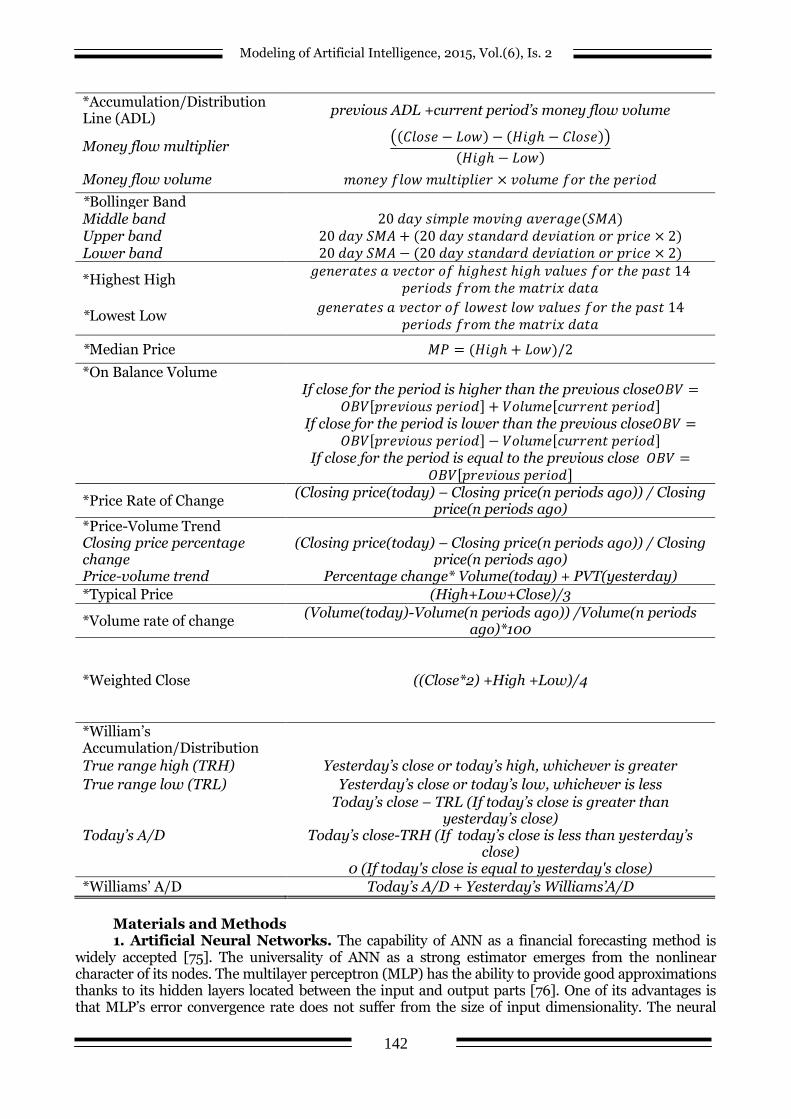
*Accumulation/Distribution Line (ADL)

previous ADL +current period’s money flow volume

Money flow multiplier 𝐶𝑙𝑜𝑠𝑒 − 𝐿𝑜𝑤 − 𝐻𝑖𝑔𝑕 − 𝐶𝑙𝑜𝑠𝑒

𝐻𝑖𝑔𝑕 − 𝐿𝑜𝑤

Money flow volume 𝑚𝑜𝑛𝑒𝑦 𝑓𝑙𝑜𝑤 𝑚𝑢𝑙𝑡𝑖𝑝𝑙𝑖𝑒𝑟 × 𝑣𝑜𝑙𝑢𝑚𝑒 𝑓𝑜𝑟 𝑡𝑕𝑒 𝑝𝑒𝑟𝑖𝑜𝑑

*Bollinger Band Middle band 20 𝑑𝑎𝑦 𝑠𝑖𝑚𝑝𝑙𝑒 𝑚𝑜𝑣𝑖𝑛𝑔 𝑎𝑣𝑒𝑟𝑎𝑔𝑒(𝑆𝑀𝐴) Upper band 20 𝑑𝑎𝑦 𝑆𝑀𝐴 + (20 𝑑𝑎𝑦 𝑠𝑡𝑎𝑛𝑑𝑎𝑟𝑑 𝑑𝑒𝑣𝑖𝑎𝑡𝑖𝑜𝑛 𝑜𝑟 𝑝𝑟𝑖𝑐𝑒 × 2) Lower band 20 𝑑𝑎𝑦 𝑆𝑀𝐴 − (20 𝑑𝑎𝑦 𝑠𝑡𝑎𝑛𝑑𝑎𝑟𝑑 𝑑𝑒𝑣𝑖𝑎𝑡𝑖𝑜𝑛 𝑜𝑟 𝑝𝑟𝑖𝑐𝑒 × 2)

*Highest High 𝑔𝑒𝑛𝑒𝑟𝑎𝑡𝑒𝑠 𝑎 𝑣𝑒𝑐𝑡𝑜𝑟 𝑜𝑓 𝑕𝑖𝑔𝑕𝑒𝑠𝑡 𝑕𝑖𝑔𝑕 𝑣𝑎𝑙𝑢𝑒𝑠 𝑓𝑜𝑟 𝑡𝑕𝑒 𝑝𝑎𝑠𝑡 14

𝑝𝑒𝑟𝑖𝑜𝑑𝑠 𝑓𝑟𝑜𝑚 𝑡𝑕𝑒 𝑚𝑎𝑡𝑟𝑖𝑥 𝑑𝑎𝑡𝑎

*Lowest Low 𝑔𝑒𝑛𝑒𝑟𝑎𝑡𝑒𝑠 𝑎 𝑣𝑒𝑐𝑡𝑜𝑟 𝑜𝑓 𝑙𝑜𝑤𝑒𝑠𝑡 𝑙𝑜𝑤 𝑣𝑎𝑙𝑢𝑒𝑠 𝑓𝑜𝑟 𝑡𝑕𝑒 𝑝𝑎𝑠𝑡 14

𝑝𝑒𝑟𝑖𝑜𝑑𝑠 𝑓𝑟𝑜𝑚 𝑡𝑕𝑒 𝑚𝑎𝑡𝑟𝑖𝑥 𝑑𝑎𝑡𝑎

*Median Price 𝑀𝑃 = (𝐻𝑖𝑔𝑕 + 𝐿𝑜𝑤)/2

*On Balance Volume

If close for the period is higher than the previous close𝑂𝐵𝑉 =

𝑂𝐵𝑉 𝑝𝑟𝑒𝑣𝑖𝑜𝑢𝑠 𝑝𝑒𝑟𝑖𝑜𝑑 + 𝑉𝑜𝑙𝑢𝑚𝑒 𝑐𝑢𝑟𝑟𝑒𝑛𝑡 𝑝𝑒𝑟𝑖𝑜𝑑

If close for the period is lower than the previous close𝑂𝐵𝑉 =

𝑂𝐵𝑉 𝑝𝑟𝑒𝑣𝑖𝑜𝑢𝑠 𝑝𝑒𝑟𝑖𝑜𝑑 − 𝑉𝑜𝑙𝑢𝑚𝑒 𝑐𝑢𝑟𝑟𝑒𝑛𝑡 𝑝𝑒𝑟𝑖𝑜𝑑

If close for the period is equal to the previous close 𝑂𝐵𝑉 =

𝑂𝐵𝑉 𝑝𝑟𝑒𝑣𝑖𝑜𝑢𝑠 𝑝𝑒𝑟𝑖𝑜𝑑

*Price Rate of Change (Closing price(today) – Closing price(n periods ago)) / Closing

price(n periods ago) *Price-Volume Trend Closing price percentage change

(Closing price(today) – Closing price(n periods ago)) / Closing price(n periods ago)

Price-volume trend Percentage change* Volume(today) + PVT(yesterday)

*Typical Price (High+Low+Close)/3

*Volume rate of change (Volume(today)-Volume(n periods ago)) /Volume(n periods

ago)*100

*Weighted Close ((Close*2) +High +Low)/4

*William’s Accumulation/Distribution

True range high (TRH) Yesterday’s close or today’s high, whichever is greater

True range low (TRL) Yesterday’s close or today’s low, whichever is less

Today’s A/D

Today’s close – TRL (If today’s close is greater than yesterday’s close)

Today’s close-TRH (If today’s close is less than yesterday’s close)

0 (If today's close is equal to yesterday's close)

*Williams’ A/D Today’s A/D + Yesterday’s Williams’A/D

Materials and Methods 1. Artificial Neural Networks. The capability of ANN as a financial forecasting method is

widely accepted [75]. The universality of ANN as a strong estimator emerges from the nonlinear character of its nodes. The multilayer perceptron (MLP) has the ability to provide good approximations thanks to its hidden layers located between the input and output parts [76]. One of its advantages is that MLP’s error convergence rate does not suffer from the size of input dimensionality. The neural


143

network can be trained by back propagation and the gradient search scheme is an efficient tool to minimize the mean squared error between the estimated and real output values. A weight adjusting system adapts the weights of the network according to the feedback of the backwards propagated data to reduce the difference between the computed value and the target value [76]. In regression calculations, errors that are squared and added together as the error function form an indicator of fit, while in classification problems the squared error together with deviance can serve as a fit function [77]. Overfitting in neural networks as it is caused by weights has always been a major obstacle in model training. In order not to reach the global minimum or prevent overfitting, early model designers relied on some sort of exit rule. Weights are designed to push the final construct of the model to have a linear solution. Meanwhile, in order to restrict the validation error growth a certain dataset for validation is utilized to decide when to stop.

The eventual result relies on input scaling which also influences the weights in the lowest layer. The number of concealed bands or layers is determined by sheer experimentation and its number usually grows with the number of input attributes. In this sense, a very efficient tool to determine the parameters of standardization or optimal concealed layer numbers is cross validation. The function of these concealed bands is to extract patterns or features in regression or classification problems. The construction of various concealed layers may possibly help to find out features of hierarchy [77].

2. Support Vector Machines. The support vector machine (SVM) method is based on a fundamental concept used in statistics that seeks to minimize the structural risk [76]. Minimizing the training error is not the aim of SVM but it seeks to increase the boundary between the training data and the dividing hyper-plane to the greatest amount or degree. The nonlinearity of kernel functions addresses well the challenge of dimensionality in data spaces. With favorable hyper-planes capable of mapping input space examples to higher dimensional spaces, better generalization is achieved. It is easier to interpret a linear or near linear high-dimensional input space which is a product of suitable mapping. At the end, the machine learning of SVM is turned into a second degree optimization problem where the there is a single global solution with linear constraints. The universality of SVM is unique in approximation for assorted kernels. The most important aspect of SVM is that there is no local minima, while learning data subsets labeled as support vector, characterize SVM. These data subsets or support vectors are compressed from the training dataset that meagerly identifies the SVM model [76]. SVM, which tries to find the suitable hyper-plane identifying the permissible difference between two classes, is a method that was proposed for classification, at the outset. If two classes can be linearly divided the most favorable hyper-plane is able to identify the permissible margin between them. Nonetheless, at some instances overlapping non-divisible classes are made linearly separable at another level or the so-called transformed feature space [77]. For this study, as the means of calculations, WEKA which is an open source machine learning device was used. The SVM-SMO (Sequential Minimal Optimization) method, which is available among WEKA options, is one of the quickest schemes used for sparse sets. SVM is capable of handling large sets while having dominance over the calculating complexity of the SVM-SMO system [76]. ―The sequential minimal optimization technique implements John Platt's algorithm to train a support vector classifier. The global implementation replaces all missing values and nominal attributes are transformed into binary ones. All attributes are normalized by default and the output coefficients are based on the normalized data but not on the original data which is crucial for interpreting the classifier‖ [78].

3. Random Forests. A great deal of work have resulted in better classification precision with bundles of trees that can decide for the prevailing class among others. To flourish those trees, supervising random vectors are usually produced to oversee the tree progression in the bundle. One way to achieve the growth of a tree is by means of bagging or the arbitrary choosing of training group examples [79]. In another scheme, which is called random split selection, an arbitrary splitting process is called in at relevant nodes [80]. It is possible to create new training groups from the primary training group by disarranging the outputs or choosing from a random group of weights in the original training set [81]. Regarding the growth of trees, [82] writes about random subspaces which are arbitrary choices of feature subsets and in another study, [82] use arbitrarily chosen geometric attributes to provide each node with the best division. The parameter in building trees is 𝑘𝑛 that provide minimal number of prediction points having to show on each leaf and 𝑛, the subscript representing the size of the training group, is a measure of the minimum leaf size against the number of training data. Prior to predicting a point of interest 𝑥, the forest needs to be trained before each tree can produce its unique estimation


144

𝑓𝑛𝑗 𝑥 =

1

𝑁𝑒 𝐴𝑛 𝑥 𝑌𝑖

𝑌𝑖𝜖𝐴𝑛 𝑥 , 𝐼𝑖=𝑒

Then the estimations of each tree are averaged by the forest

𝑓𝑛 𝑀

𝑥 =1

𝑀 𝑓𝑛

𝑗

𝑀

𝑗 =1

𝑥

where 𝐴𝑛 𝑥 represents the leaf holding 𝑥 and 𝑁𝑒 𝐴𝑛 𝑥 shows the number of prediction

points that it holds. It should be noted that each tree’s estimation is only bound by the prediction points in that tree. On the other hand, despite the fact that each tree’s points are attached to the estimation structure independently, one tree’s points could be instrumental in the prediction as being estimation points in another tree [84-85].

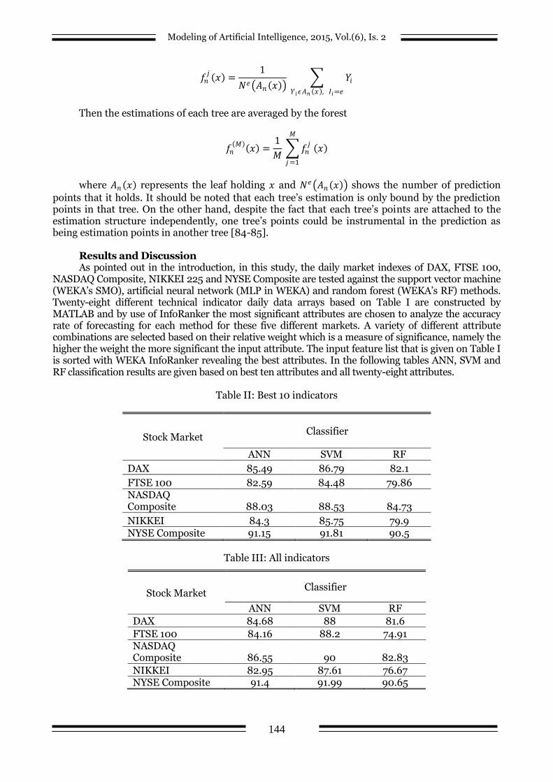
Results and Discussion As pointed out in the introduction, in this study, the daily market indexes of DAX, FTSE 100,

NASDAQ Composite, NIKKEI 225 and NYSE Composite are tested against the support vector machine (WEKA’s SMO), artificial neural network (MLP in WEKA) and random forest (WEKA’s RF) methods. Twenty-eight different technical indicator daily data arrays based on Table I are constructed by MATLAB and by use of InfoRanker the most significant attributes are chosen to analyze the accuracy rate of forecasting for each method for these five different markets. A variety of different attribute combinations are selected based on their relative weight which is a measure of significance, namely the higher the weight the more significant the input attribute. The input feature list that is given on Table I is sorted with WEKA InfoRanker revealing the best attributes. In the following tables ANN, SVM and RF classification results are given based on best ten attributes and all twenty-eight attributes.

Table II: Best 10 indicators

Table III: All indicators

Stock Market Classifier

ANN SVM RF

DAX 85.49 86.79 82.1

FTSE 100 82.59 84.48 79.86 NASDAQ Composite 88.03 88.53 84.73

NIKKEI 84.3 85.75 79.9 NYSE Composite 91.15 91.81 90.5


ANN SVM RF

DAX 84.68 88 81.6

FTSE 100 84.16 88.2 74.91 NASDAQ Composite 86.55 90 82.83

NIKKEI 82.95 87.61 76.67 NYSE Composite 91.4 91.99 90.65


145

Table IV: Difference in % (table II values with respect to table III values)

Table II and Table III show results obtained by WEKA. DAX, FTSE 100, NASDAQ

Composite, Nikkei and NYSE Composite indexes represent five different stock markets worldwide. Table IV displays the % difference of accuracy values using the best ten indicators (Table II) in relation to all indicators (Table III). While the multilayer perceptron (ANN) is producing relatively better outcomes for DAX, NASDAQ and NIKKEI, the results for FTSE 100 and NYSE are less accurate. In the SVM category all results show better predictability of SVM when all indicators are used. Random forest is clearly having better forecasting capability with best ten indicators for FTSE, NASDAQ and NIKKEI indexes. The best ten indicators show a stronger forecasting power with random forest than when all inputs are used. In case of FTSE 100, NIKKEI, NASDAQ Composite and DAX, random forest fed with best ten inputs has a better prediction ability than random forest fed with all inputs given in Table I. On the other hand, it is interesting to see SVM fed with all technical indicators, showing higher accuracy rates than when it is fed by the best ten indicators. From Table II and Table III, it can be drawn that SVM is the better estimator compared to ANN and RF. When Table IV is examined, DAX, NASDAQ Composite and NIKKEI indexes show similar classification result pattern when subjected to either the best ten or all technical indicators given in Table I, i.e. they response in the same way to the three different estimators (ANN, SVM and RF) when the number of attributes are changed.

Conclusion In this article, it is aimed to find out the accuracy estimation responses of five different stock

market indexes, namely DAX, NIKKEI 225, NYSE Composite, NASDAQ composite and FTSE 100, to the SVM, ANN and random forest classifiers. Keeping in mind that no stock market is a perfect financial system whose daily movement direction can be absolutely precisely forecasted, professionals and researchers in finance alike are working on finding efficient ways to make sound and sustainable predictions that will serve as a basis for market decisions. Statistical methods like ARMA, GARCH and ARIMA have been around for a while, though none guarantees sustainability and reliability forever. In finance, it is a fact that there is no single solution to different financial questions, especially for systems as volatile as stock markets. One forecasting method could work better than the other for different time-dependent datasets or market indexes, with different feature sets and different parameters of the same estimation scheme. The forecasting schemes or estimation classifiers used in this article have also been around for a while and there is actually an abundance of literature available regarding support vector machines, artificial neural networks and random forest methods. While this study is testing the prediction power of the methods used for five different market indexes, it is also comparing the classification accuracy results of the best ten most significant attributes versus all technical indicator inputs listed on Table I for each market and each test method. The results obtained in Table II and Table III show that the SVM classifier is more powerful in predicting movement directions based on daily data. As an example, SVM classified the NYSE Composite moving direction with % 91.99 and %91.81 accuracy rate, compared to ANN’s % 91.15 and % 91.4 or random forest’s % 90.5 and % 90.65. It is also interesting to see the pattern of classification results of DAX, NASDAQ Composite and NIKKEI indexes when tested with the best ten or all technical indicators given in Table I. According to this pattern, all three markets showed better classification results when tested with ANN and random forest based on the best ten


ANN SVM RF

DAX +0.96 -1.38 0.61

FTSE 100 -1.86 -4.22 6.61 NASDAQ Composite

+1.71 -1.63 2.29

NIKKEI +1.63 -2.12 4.21 NYSE Composite -0.27 -0.20 -0.16


146

technical indicators. On the other hand when they are tested with SVM based on all technical indicators given on Table I they showed lower accuracy results. This study can be furthered using other stock market indexes with other data mining techniques fed with different technical indicator sets to see if these techniques can achieve better accuracy rates or if some similar classification result pattern of these market indexes can be obtained. Then a more elaborate experimentation on part of the markets with similar pattern may inspire researchers to find which technique and input set would best serve to make sound decisions for a particular bundle of markets.

References: 1. Bisoi R. and Dash P.K. (2014) A hybrid evolutionary dynamic neural network for stock

market trend analysis and prediction using unscented Kalman filter, Applied Soft Computing, 19, 41-56.

2. Sun Y. F., Liang Y. C., Zhang W. L., Lee H. P. and Lin W. Z. (2005) Optimal partition algorithm for the RBF neural network for financial time series forecasting, Neural Computing and Applications 14, 36-44.

3. Yumlu S., Gurgen F. G. and Okay N. (2005) A Comparison of global, recurrent and smoothed-piecewise neural models for Istanbul stock exchange prediction, Pattern Recognition Letters 26, 2093–2103.

4. Qi M. and Zhang G. P. (2003) Trend time series modeling and forecasting with neural networks, IEEE International Conference on Computational Intelligence for Financial Engineering, pp. 331–337.

5. Bildirici M. and Ersin O. (2009) Improving forecasts of GARCH family models with the artificial neural networks: an application to the daily returns in Istanbul stock exchange, Expert System with Applications 36, 7355–7362.

6. Majhi R., Panda G. and Sahoo G. (2009) Development and performance evaluation of FLANN based model for forecasting stock market, Expert systems with Applications 36, 6800-6808.

7. Chen Y., Yang B. and Dong J. (2006) Time series prediction using a local linear wavelet neural network, Neurocomputing 69, 449-465.

8. Zhao Y., Zhang Y. and Qi C. (2008) Prediction model of stock market returns based on wavelet neural network, in Asia Pacific Workshop on Computational Intelligence and Industrial Application, pp. 31-36.

9. Liu C. F., Yeh C. Y. and Lee S. J. (2012) Application of type-2 neuro-fuzzy modeling in stock price prediction, Applied Soft Computing, 1348-1358.

10. Wei L. Y., Chen T. L. and Ho T. H. (2011) A hybrid model based on adaptive-network-based fuzzy inference system to forecast Taiwan stock market, Expert Systems with Applications 38 (1), 13625-21363.

11. Chang P. C. and Fan C. Y. (2008) A hybrid system integrating a wavelet and TSK fuzzy rules for stock price forecasting, IEEE Transactions on Man, Machine, and Cybernetics: Part C 38, 802-815.

12. Wang Y., Cai Z. and Zhang Q. (2011) Differential evolution with composite trial vector generation strategies and control parameters, IEEE Transactions on Evolutionary Computation 15, 55-66.

13. Huang F. Y. (2008) Integration of an improved particle swarm optimization algorithm and fuzzy neural network for Shanghai stock market prediction, in: IEEE Workshop on Power Electronics and Intelligent Transportation System.

14. Menezes M. L. and Nikolaev N. Y. (2006) Forecasting with genetically programmed polynomial networks, Int. J. Forecast., 249-165.

15. Fajiang L. and Jun W. (2012) Fluctuation prediction of stock market index by Legendre neural network, Neurocomputing 83, 12-21.

16. Pan H. (2003) Proc. 2003 Hawaii International Conference on Statistics and Related Fields.

17. Fama E. F. (1970) Efficient capital markets: a review of theory and empirical work, J.Finance 25, 383-417.

18. Granger C. J. (1989) Combining forecasts – twenty years later, J. Forecast. 8, 167-173.


147

19. Ginzburg I. and Horn D. (1994) Combined neural networks for time series analysis, Adv. Neural Inform. Process. Syst. 6, 224-231.

20. Bollerslev T. (1986) Generalized autoregressive conditional heteroscedasticity, J. Econometrics 31, 307-327.

21. Hsieh D. A. (1991) Chaos and nonlinear dynamics: application to financial markets, J. Finance 46, 1839-1877.

22. Box G. E., Jenkins G. M. and Reinsel G. C. (1994) Time Series Analysis: Forecasting and Control, New Jersey: Prentice Hall.

23. Engle R. F. (1982) Autoregressive conditional heteroskedasticity with estimates of the variance of UK inflation, Econometrica 50, 987-1008.

24. Rao T. S. and Gabr M. M. (1984) Introduction to Bispectral Analysis and Bilinear Time Series Models, Lecture Notes in Statistics, Springer vol.24.

25. Ozaki T. (1985) Nonlinear Time Series Models and Dynamical Systems, Amsterdam: Handbook of Statistics, vol. 5, North Holland.

26. Clements M. P., Franses P. H. and Swanson N. R. (2004) Forecasting economic and financial time-series with non-linear models, Int. J. Forecast. 20, 169-183.

27. Priestley M. B. (1988) Non-Linear and Non-Stationary Time Series Analysis, Academic Press.

28. Hadavandi E., Shavandi A. and Ghanbari A. (2010) Integration of genetic fuzzy systems and artificial neural networks for stock price forecasting, Knowl.Based Syst. 23, 800-808.

29. Hadavandi E., Ghanbari A. and Naghneh S. (2010) Developing a time series model based on particle swarm optimization for gold price forecasting, in: Third International Conference on Business Intelligence and Financial Engineering, pp.337-340.

30. Lee Y. and Tong L. (2011) Forecasting time series using a methodology based on autoregressive integrated moving average and genetic programming, Knowl. Based Syst. 24, 66-72.

31. Asadi S., Tavakoli A. and Hejazi S. R. (2012) A new hybrid for improvement of autoregressive integrated moving average models applying particle swarm optimization, Expert Syst. Appl. 39 (5), 5332-5337.

32. Chang P. C. and Liu C. H. (2008) A TSK type fuzzy rule based system for stock price prediction, Expert Syst. Appl. 34, 135-144.

33. Esfahanipour A. and Aghamiri W. (2010) Adapted neuro-fuzzy inference system on indirect approach TSK fuzzy rule base for stock market analysis, Expert Syst. Appl. 37, 4742-4748.

34. Shen W., Guo X., Wu C. and Wu D. (2011) Forecasting stock indices using radial basis function neural networks optimized by artificial fish swarm algorithm, Knowl. Based Syst. 24, 378-385.

35. De A. and Araujo R. (2011) A class of hybrid morphological perceptrons with application in time series, Knowl. Based Syst. 24, 513-529.

36. Cho V. (2010) MISMIS-A comprehensive decision support system for stock market investment, Knowl. Based Syst. 23, 626-633.

37. Chang Chien Y.W. and Chen Y. L. (2010) Mining associative classification rules with stock trading data-A GA-based method, Knowl. Based Syst. 23, 605-614.

38. Asadi S., Hadavandi E. and Mehmanpazir F. (2012) Hybridization of evolutionary Levenberg–Marquardt neural networks and data, Knowledge-Based Systems 35, 245-258.

39. Hagan M. and Menhaj M. (1994) Training feedforward networks with the marquardt algorithm, IEEE TNN. 5 (6), 989-993.

40. Bartlett P. and Downs T. A. (1990) Training a Neural Network with a Genetic Algorithm, Dept. of Electrical Engineering, University of Queensland.

41. Yao X. (1999) Evolving artificial neural networks, in: Proceedings of the IEEE. 42. Knowles J. D. and Corne D. W. (2001) Evolving neural networks for cancer radiotherapy,

in: The Practical Handbook of Genetic Algorithms Applications, Chapman & Hall/CRC. 43. Chang P. C., Wang Y. W. and Tsai C. Y. (2005) Evolving neural network for printed circuit

board sales forecasting, Expert Syst. Appl. 29, 83-92. 44. Kuo R. J. and Chen J. A. (2004) A decision support system for order selection in

electronic commerce based on fuzzy neural network supported by real-coded genetic algorithm, Expert Syst. Appl. 26, 141-154.

45. Sexton R. S. and Gupta J. N. (2000) Comparative evaluation of genetic algorithm and back-propagation for training neural networks, Inform. Sci. 129, 45-59.


148

46. Maragos P. (1989) A representation theory for morphological image and signal processing, IEEE Transactions on Pattern Analysis and Machine Intelligence, 11, 586-599, 1989.

47. Coyle E. J. and Lin J. H. (1988) Stack filters and the mean absolute error criterion, IEEE Transactions on Acoustics, Speech and Signal Processing, 36, 1244-1254.

48. Herwing C. B. and Shalkoff R. J. (1994) Morphological image processing using artificial neural networks, Academic Press, Vol. 67, pp. 319–379.

49. Pessoa L. C. and Maragos P. (1998) MRL-filters: A general class of nonlinear systems and their optimal design for image processing, IEEE Transactions on Image Processing, 7, 966-978.

50. Pessoa L. C. and Maragos P. (2000) Neural networks with hybrid morphological/ rank/linear nodes: A unifying framework with applications to handwritten character recognition, Pattern Recognition, 33, 945-960.

51. Ane T., Ureche-Rangau L., Gambet J.-B. and Bouverot J. (2008) Robust outlier detection for Asia-Pacific stock index returns, Journal of International Financial Markets Institutions and Money, 18(4), 326-343.

52. Kim J. H. and Shamsuddin A. (2008) Are Asian stock markets efficient? Evidence from new multiple variance ratio tests, Journal of Empirical Finance, 15, 518-532.

53. Mazouz K., Joseph N. L. and Palliere C. (2009) Stock index reaction to large price changes: Evidence from major Asian stock indexes, Pacific-Basin Finance Journal, 17(4), 444-459.

54. Atsalakis G. S. and Valavanis K. (2009) Surveying stock market forecasting techniques-Part II: Soft computing methods, Expert systems with Applications, 36(3), 5932-5941.

55. Huang W., Nakamori Y. and Wang S. Y. (2005) Forecasting stock market movement direction with support vector machine, Computers & Operations Research, 32(10), 2513-2522.

56. Lee T. S. and Chen N. J. (2002) Investigating the information content of non-cash trading index futures using neural networks, Expert Systems with Applications, 22(3), 255-234.

57. Lu C. J. (2010) Integrating independent component analysis-based denoising scheme with neural network for stock price prediction, Expert Systems with Applications , 37(10), 7056-7064.

58. Lu C. J., Lee T. S. and Chiu C. C. (2009) Financial time series forecasting using independent component analysis and support vector regression, Decision Support Systems, 47(2), 115-125.

59. Cao Q., Leggio K. B. and Schniederjans M. J. (2005) A comparison between Fama and French's model and artificial neural networks in predicting the Chinese stock market, Computers & Operations Research, 32(10), 2499-2512.

60. Vellido A., Lisboa P. J. and Vaughan J. (1999) Neural networks in business: A survey of applications (1992-1998), Expert Systems with Applications, 17, 51-70.

61. Zhang G., Patuwa B. E. and Hu M. Y. (1998) Forecasting with artificial neural networks: The state of the art, International Journal of Forecasting, 14, 35-62.

62. Back A. and Weigend A. (1997) Discovering structure in finance using independent component analysis, in Proceeding of fifth international conference on neural networks in capital market, pp. 15-17.

63. Gorriz L. M., Puntonet C. G., Salmeron M. and Lang E. (2003) Time series prediction using ICA algorithms, Computing International Scientific Journal, 2(2), 69-75, 2003.

64. Kiviluoto K. and Oja E. (1998) Independent component analysis for parallel financial time series, in Proceedings of the fifth international conference on neural information, pp. 895-898, Tokyo, Japan.

65. Malaroiu S., Kiviluoto K. and Oja E. (2000) Time series prediction with independent component analysis, in Proceedings of international conference on advanced investment technology, pp. 895-898, Gold Coast, Australia.

66. Mok P. Y. , Lam K. P. and Ng H. S. (2004) An ICA design of intraday stock prediction models with automatic variable selection, in Proceedings of 2004 IEEE international joint conference on neural networks, pp. 2135-2140, Budapest, Hungary.

67. Hyvarinen A., Karhunen J. and Oja E. (2001) Independent component analysis, New York: John Wiley & Sons, 2001.

68. Almeida L. B. (2003) MISEP-Linear and nonlinear ICA based on mutual information, Journal of Machine Learning Reaching , 4, 1297-1318.


149

69. Hyvarinen A. and Pajunen P. (1999) Nonlinear independent component analysis: Existence and uniqueness results, Neural Networks, 12(3), 429-439.

70. Valpola H. (2000) Nonlinear independent component analysis using ensemble learning: Theory, in Proceedings of second international workshop on independent component analysis and blind signal seperation, pp. 251-256, Helsinki, Finland.

71. Cao L. J. and Chong W. K. (2002) Feature extraction in support vector machine: a comparison of PCA, XPCA and ICA, in Proceedings of the ninth international conference on neural information, 2, pp. 1001-1005.

72. Haritopoulus M., Yin H. and Allinson N. M. (2002) Image denoising using self-organizing map-based nonlinear independent component analysis, Neural Networks, 15, 1085-1098.

73. Zhang K. and Chan L. (2007) Nonlinear independent component analysis with minimal nonlinear distortion, in Proceedings of the 24th international conference on Machine Learning, pp. 1127-1134, Oregon, USA.

74. Colby R. W. (2003) The Encyclopedia of Technical Market Indicators, McGraw-Hill. 75. Kara Y., Boyacioglu M. A. and Baykan O. K. (2010) Predicting direction of stock price

index movement using artificial neural networks and support vector machines: The sample of the Istanbul Stock Exchange, Expert Systems with Applications 38, 5311–5319.

76. Du K. L. and Swamy M. N. S. (2006 ) Neural Networks in a Softcomputing Framework, Springer-Verlag.

77. Hastie T., Tibshirani R. and Friedman J. (2008) The Elements of Statistical Learning, Springer, 2nd. Edition.

78. Weka (1999-2010) Waikato Environment for Knowledge Analysis, Version 3.7.3, The University of Waikato Hamilton, New Zealand.

79. Breiman L. (1999) Random Forests-Random Features, Statistics Dept. University of California, Berkeley.

80. Dietterich T. G. (2009) Machine Learning in Ecosystem Informatics and Sustainability, Proceedings of the 2009 International Joint Conference on Artificial Intelligence.

81. Ho T. K. (1998) The Random Subspace Method for Constructing Decision Forests, IEEE Transactions on Pattern Analysis and Machine Intelligence, pp. 832-844.

82. Amit Y. and Geman D. (1997) Shape Quantization and Recognition with Randomized Trees, Neural Computation, 9, 1545-1588.

83. Breiman L. (2001) Random Forests, Statistics Dept. University of California, Berkeley. 84. Denil M., Matheson D. and Freitas N. (2014) Narrowing the Gap: Random Forests in

Theory and in Practice, Journal of Machine Learning Research. 85. Denil M, Matheson D. and Freitas N. (2013) Narrowing the Gap: Random Forests in

Theory and in Practice, Journal of Machine Learning Research.

copyright © 2015 by academic publishing house...

Documents