copy of thesis backup7 - texas a&m...
TRANSCRIPT
STATISTICAL ESTIMATION OF WATER DISTRIBUTION SYSTEM PIPE
BREAK RISK
A Thesis
by
SHRIDHAR YAMIJALA
Submitted to the Office of Graduate Studies of Texas A&M University
in partial fulfillment of the requirements for the degree of
MASTER OF SCIENCE
August 2007
Major Subject: Civil Engineering
STATISTICAL ESTIMATION OF WATER DISTRIBUTION SYSTEM PIPE
BREAK RISK
A Thesis
by
SHRIDHAR YAMIJALA
Submitted to the Office of Graduate Studies of Texas A&M University
in partial fulfillment of the requirements for the degree of
MASTER OF SCIENCE
Approved by: Co-Chairs of Committee, Seth Guikema Kelly Brumbelow Committee Member, Ruzong Fan Head of Department, David Rosowsky
August 2007
Major Subject: Civil Engineering

iii
ABSTRACT
Statistical Estimation of Water Distribution System Pipe Break Risk. (August 2007)
Shridhar Yamijala, B.E., Government College of Engineering Pune, India
Co-Chairs of Advisory Committee: Dr. Seth Guikema Dr. Kelly Brumbelow
The deterioration of pipes in urban water distribution systems is of concern to water
utilities throughout the world. This deterioration generally leads to pipe breaks and
leaks, which may result in reduction in the water-carrying capacity of the pipes from
tuberculation of interior walls of the pipe. Deterioration can also lead to contamination
of water in the distribution systems. Water utilities which are already facing tight
funding constraints incur large expenses in replacement and rehabilitation of water
mains, and hence it becomes critical to evaluate the current and future condition of the
system for making maintenance decisions. Quantitative estimates of the likelihood of
pipe breaks on individual pipe segments can facilitate inspection and maintenance
decisions. A number of statistical methods have been proposed for this estimation
problem. This thesis focuses on comparing these statistical models on the basis of short
time histories. The goals of this research are to estimate the likelihood of pipe breaks in
the future and to determine the parameters that most affect the likelihood of pipe breaks.
The various statistical models reviewed in this thesis are time linear and time
exponential ordinary least squares regression models, proportional hazards models
(PHM), and generalized linear models (GLM). The data set used for the analysis comes

iv
from a major U.S. city, and the data includes approximately 85,000 pipe segments with
nearly 2,500 breaks from 2000 through 2005. The covariates used in the analysis are
pipe diameter, length, material, year of installation, operating pressure, rainfall, land use,
soil type, soil corrosivity, soil moisture, and temperature. The Logistic Generalized
Linear Model fits can be used by water utilities to choose inspection regimes based on a
rigorous estimation of pipe breakage risk in their pipe network.

v
ACKNOWLEDGEMENTS
I would like to express my sincere gratitude towards my thesis advisor, Dr. Seth
Guikema, for his valuable guidance throughout my graduate studies and his technical
input during the course of this research effort. I also wish to thank my committee
members Dr. Kelly Brumbelow for providing the data for this research and Dr. Ruzong
Fan for agreeing to serve on my committee and for providing valuable suggestions on
improving this research in various ways.
I am grateful to Dr. Wood from the University of Washington for providing me
with the soil moisture data. I would like to specially thank David Wolter for his ArcGIS
support. I sincerely acknowledge the valuable suggestions of other members of the
“Infrastructure Risk, Reliability, and Sustainability Research Group” that include Jeremy
Coffelt, Seung Ryong Han, Roshan Pawar, William Imbeah, and Neethi Rajagopalan. I
also cannot forget the encouragement offered to me by my roommates and my friends.
Finally, I would like to thank my parents and my brother Gopal for their advice
and support throughout my graduate studies.

vi
TABLE OF CONTENTS
Page
ABSTRACT ..................................................................................................................... iii
ACKNOWLEDGEMENTS............................................................................................... v
TABLE OF CONTENTS ................................................................................................. vi
LIST OF FIGURES ........................................................................................................ viii
LIST OF TABLES............................................................................................................. x
1. INTRODUCTION..................................................................................................... 1
1.1. Causes and effects of pipe failures ............................................................ 3 1.2. Physical modeling of pipe breakages ........................................................ 5 1.3. Difference between pipe breaks and leaks ................................................ 6 1.4. Objectives of research ............................................................................... 8
2. LITERATURE REVIEW........................................................................................ 11
2.1. Introduction ............................................................................................. 11 2.2. Past statistical studies .............................................................................. 11 2.3. Predictive statistical models for pipe break failures ................................ 14 2.3.1. Aggregate type models ............................................................................ 15 2.3.2. Introduction to multiple regression type models ..................................... 16
3. DATA DESCRIPTION ........................................................................................... 32
3.1. Principal components analysis................................................................. 34 3.2. A sample of the dataset............................................................................ 36
4. MODEL DESCRIPTION........................................................................................ 42
4.1. Time linear model.................................................................................... 42 4.2. Time exponential model .......................................................................... 43 4.3. Poisson generalized linear model ............................................................ 43 4.4. Logistic generalized linear model............................................................ 44 4.5. Methodology............................................................................................ 45

vii
Page
5. RESULTS................................................................................................................ 50
5.1. Time linear model.................................................................................... 50 5.1.1. Hypothesis testing using likelihood ratio statistic ................................... 55 5.1.2. Relative effects of variables .................................................................... 56 5.1.3. Holdout sample analysis results .............................................................. 58 5.1.4. Random holdout sample analysis ............................................................ 60
5.2. Time exponential model .......................................................................... 61 5.2.1. Holdout sample analysis results .............................................................. 64 5.2.2. Random holdout sample analysis ............................................................ 65
5.3. Poisson generalized linear model ............................................................ 66 5.3.1. Hypothesis testing.................................................................................... 67 5.3.2. Relative effects of variables .................................................................... 70 5.3.3. Holdout sample analysis .......................................................................... 72 5.3.4. Random holdout sample analysis ............................................................ 73
5.4. Logistic generalized linear model............................................................ 77 5.4.1. Random holdout sample analysis ............................................................ 79
5.5. Comparison of Poisson GLM and Logistic GLM ................................... 81 5.6. Summary.................................................................................................. 83
6. DISCUSSION.......................................................................................................... 85
6.1. Applications of the logistic GLM............................................................ 85 6.2. Applications to other systems.................................................................. 86 6.3. Limitations in analysis............................................................................. 87 6.4. Suggestions for future research ............................................................... 88
7. CONCLUSION ....................................................................................................... 90
REFERENCES……………………………………………………………………… 92 APPENDIX A.................................................................................................................. 98
APPENDIX B................................................................................................................ 100
VITA.............................................................................................................................. 104

viii
LIST OF FIGURES
FIGURE Page
1. Failure modes for buried pipes: direct tension (top left), bending or flexural failure (middle), and hoop stress (bottom) (Taken from Rajani and Kleiner, 2001) .............................................................................................. 7
2. Histograms of some variables........................................................................... 40
3. Scatter plot of number of pipe breaks against diameter of pipes, length of pipes, pressure in pipes, year of installation of pipes, time since last break on the pipes, and rainfall......................................................................... 41
4. Time linear model predictions.......................................................................... 53
5. Q-Q plot for residuals of TLM ......................................................................... 53
6. Cook’s distance for time linear model.............................................................. 54
7. Relative effects of covariates in the time linear model .................................... 58
8. Holdout sample results for time linear model .................................................. 59
9. Random holdout sample analysis of time linear model.................................... 61
10. Time exponential model predictions ................................................................ 63
11. QQ plot for time exponential model................................................................. 63
12. Holdout sample analysis for time exponential model ...................................... 64
13. Random holdout sample analysis for time exponential model......................... 65
14. Poisson generalized linear model predictions .................................................. 70
15. Relative effects of variables for Poisson GLM ................................................ 72
16. Holdout sample analysis plot............................................................................ 73
17. Random holdout sample analysis of Poisson GLM.......................................... 74
18. Probability of having one or more breaks for Poisson GLM ........................... 82
ix
FIGURE Page
19. Probability of having no breaks or more than one break for logistic generalized linear model................................................................................... 82
20. Plot of ranking of pipes against fraction of pipes at or above the rank
that had a break................................................................................................. 86

x
LIST OF TABLES
TABLE Page
1. General characteristics of leaks and breaks (Mays, L., 2000) ............................... 7 2. Number of failures per kilometer per year for various pipe sizes and types
in 4 cities (Kettler and Goulter, 1985) ................................................................. 20 3. A sample of the dataset used in the analysis ....................................................... 37 4. Summary of input data ........................................................................................ 38 5. Parameter significance results for time linear model. ......................................... 52 6. Hypothesis tests for time linear model ................................................................ 56 7. Hypothesis tests for Poisson generalized linear model ....................................... 68 8. Parameter significance results for Poisson generalized linear model.................. 69 9. Goodness of fit statistics for all models............................................................... 75 10. Mean square error for holdout sample analysis of all models ............................. 75 11. Mean square error for random holdout sample analysis of all models................ 76 12. Parameter significance results for logistic generalized linear model .................. 80

1
1. INTRODUCTION
The progressive decay of the nation’s infrastructure systems such as
transportation, water supply, and sewer systems together with the burgeoning public
awareness about this deterioration creates the need for more scientific studies to
understand the failure patterns of infrastructure systems and propose methodologies to
reduce the number of failures. All these systems constitute the infrastructure of urban
centers, and water distribution systems play a critical role in the successful functioning
of a city. Community public health standards and the drive for future growth and
economic development are heavily dependent upon the condition of water mains and the
services they provide.
The deterioration of pipes in urban water distribution systems presents a major
challenge to water utilities throughout the world. Pipe deterioration can lead to pipe
breaks and leaks, which may result in a reduction in the water carrying capacity of pipes
and lead to substantial repair costs. Pipe breaks can also pose potential dangers by
temporarily reducing fire fighting capabilities and contaminating water in distribution
systems. These problems are responsible for increasing future repair and pumping costs,
irregular services, potential for damage caused by breaks, for example flooding, traffic
interruptions and functioning of other utilities, and problems of water quality due to
manifestation of bacteria in the tubercles formed in the interiors of pipe walls1(Andreou,
This thesis follows the style of Risk Analysis.

2
1986). Solutions for the above problems include either replacing or rehabilitating (i.e.
cleaning and lining) affected sections of pipes in the system.
The investment in maintaining and repairing pipes represents a major portion of
the expenditure of water utilities. According to Kleiner and Rajani (2001), distribution
networks often account for up to eighty percent of the total expenditure involved in
water supply systems. Furthermore, Stratus Consulting (1998) indicated that
approximately $325 billion is needed for replacement and rehabilitation of water
distribution systems across the United States.
If abundant resources were available, it would not be a problem to renew and
rehabilitate potable water distribution systems. However, the scarcity of resources
necessitates the search for the most cost effective renewal or rehabilitation strategy.
Before making decisions related to repair and rehabilitation for deteriorating pipelines,
there is a need to develop an understanding about the failure mechanisms and factors
contributing to pipe breaks. Pipe material, the environment in which the pipes are laid
and the operating characteristics of the system combine to influence the likelihood of
pipe breaks. Morris (1967) suggested a few possible causes of water main structural
failures that include soil aggressiveness or corrosivity, soil stability, weather conditions,
bedding conditions, construction quality and land development. Some other factors
responsible for pipe failures include internal corrosion, pressure surges, and faulty
anchorages at branches, bends and dead ends. Shamir and Howard (1979) extended the
list to include manufacturing flaws, traffic loading, pressure and water hammer. Marks et
al. (1987) raised the importance of joints leading to structural failure. The U.S. Army

3
Corps of Engineers (1980) found that prior leakage increased the moisture content of the
surrounding soil and promoted corrosion when they conducted a study of the New York
water supply system. Clark et al. (1988) analyzed break rates due to freezing ground
conditions.
1.1. Causes and Effects of Pipe Failures
Some causes and effects of common pipe failures have been described by Mavin
(1996). These include:
1) Pipe manufacturing defects: Inclusions, discontinuities or sporadic processing
problems. Dimensional irregularities particularly in jointing areas.
2) Storage and handling: Stress deformation due to poor stacking or storage. Cuts
or scratches on pipe walls or coatings. Impact cracks due to dropping or striking.
UV degradation, over-weathering or contamination. Inadvertent mixing of pipe
class or jointing material.
3) During construction: Poor laying, jointing or tapping techniques. Excessive
overburden/soil slips causing distortion. Construction traffic. Groundwater
flooding.
4) Subsequent works: Superimposed loadings, impacts or cover reduction. Side
slips, service pulling or moling. Loss of support or bedding.
5) Soil movement: Subsidence due to mining, filled land etc. Differential
consolidation or geological changes. Changes in water table or soil moisture
content. Extremes of climate such as frost heave or clay shrinkage. Loss of

4
anchorage/support (horizontal or vertical). Shock waves such as seismic, blasting
or vibration.
6) Soil environment: Poor original bedding/backfill. Point loads. Migration of
bedding or sidefill material. External chemical attack from natural soil. Chemical
attack due to spillages. Deterioration of the joint sealing ring(s).
7) Impact damage: Strike with bucket, pick or point (includes pulling). Point
bearing in bedding or surround. Traffic loading causing fatigue or joint
movement.
8) Temperature changes: Excess compression, end crushing. Pull out or separation
of joint. Pipe blockages and splits.
9) Internal pressure: Excess testing pressure. Pressure surge, water separation, and
vacuum collapse. Pipe tapping whilst under bending stress.
10) Others: Aggressive waters causing internal deterioration. Galvanic corrosion due
to dissimilar metals.
Complications arise when one tries to analyze and predict the future behavior of
individual pipes in a system. This is because there exists a high degree of variability in
the failure patterns of different water distribution systems and also among the pipes of a
given system. For making maintenance decisions, analysis at the individual pipe level is
required subject to particular economic and reliability criteria. The information about
structural integrity of water mains could be revealed by observing the physical condition
of water mains onsite. However, such inspection would be beneficial only if there is
presence of severe deterioration. In reality, the inspection of particular points along the

5
pipe length cannot really capture the localized nature of the various factors contributing
to breaks, their interactions and the effects of aging of the system.
Most of the times, water utilities must make inspection and maintenance
decisions about each pipe segment in their network on the basis of incomplete
information about pipe status. Hence arises the need for analyzing historical records of
pipe breaks and make use of the data concerning pipe characteristics and external
environment conditions. The estimation of future break events for each individual pipe
can serve many purposes. Taking into account the various replacement and rehabilitation
strategies, the budgetary needs for future repairs can be determined. An economic
assessment can be performed to determine optimum replacement time for affected
mains. Depending on the position of certain pipes in the network and the potential
damages associated with their failures, the estimates of reliability of individual pipe
segments can be determined.
1.2. Physical Modeling of Pipe Breakages
The physical mechanisms that drive pipe breakage are complex. They are driven
by three principal aspects: a) pipe structural properties, material type, pipe soil
interaction, and quality of installation, b) internal loads due to operational pressure and
external loads due to soil overburden, traffic loads, frost loads and third party
interference, and c) material deterioration due largely to the external and internal
chemical, biochemical and electro-chemical environment (Rajani and Kleiner, 2001).
Figure 1 graphically illustrates the failure modes for buried pipes.

6
Physical modeling of individual pipes can provide strong inferences about pipe
condition if sufficient data about the pipes is available. However, because pipes are
buried, it is prohibitively difficult to gather the information needed for physical models
of every pipe in a given water distribution system. According to Kleiner and Rajani
(2001), physical models cannot be realistically applied to assess the structural resiliency
of each individual pipe in most cases because accurate data are rarely available and are
very costly to obtain. Physical models are most often used only for the largest pipes that
are most critical to system integrity. Examples of these physical models are the frost load
model developed by Rajani and Zhan (1996), pipe-soil interaction analysis (Rajani et al.
1996), residual structural resistance analysis (Kiefner and Vieth, 1989) and the corrosion
status index of Kumar et al. (1984).
1.3. Difference between Pipe Breaks and Leaks
There is a need to distinguish between breaks and leaks when it comes to
modeling water distribution system reliability. The terms ‘leak’ and ‘break’ are used in
different ways by water utility personnel. They do not have standard definitions. In
general, a break in a main requires emergency repair whereas a leak does not. Also,
evidence of a break is obvious unlike detection of a leak which requires special
equipment. Table 1 gives the distinguishing characteristics between leaks and breaks.

7
Figure 1. Failure modes for buried pipes: direct tension (top left), bending or flexural failure
(middle), and hoop stress (bottom) (Taken from Rajani and Kleiner, 2001)
Table 1. General characteristics of leaks and breaks (Mays, L., 2000)
Sr. No. Leak Break
1. Scheduled repairs are possible Requires emergency repair
2. Specific means of detection are necessary
Detection is obvious (e.g. surfacing water, low pressure)
3. Repair does not usually interrupt service
Repair requires service shut down
4. More frequently occurs at pipe joints and service lines
Often occurs along the pipe barrel

8
Breaks result in a clear disruption of service and require some kind of repair
action whereas leaks are associated with the term ‘unaccounted for water’ and represent
a different category of pipe failures, different from breaks. Usually, the largest portion of
unaccounted for water is lost through main leaks. Yet, the popular belief is that leaks are
associated with breaks, because they can weaken the bedding material beneath the pipes
and create localized concentration of stresses. There also exists a difference between
breaks in small (less than or equal to six inches) pipes and larger pipes. The breaks in
smaller pipes are more frequent, mostly circumferential in nature, whereas those in
larger pipes are longitudinal in nature. The breaks in larger pipes are more consequential
when it comes to impacting the quality of service offered by the water utilities to its
customers. They generally result in traffic disruptions, flooding on streets and in
basements, interference with the operations of other utilities such as gas pipelines,
sewers, cable lines, and interruptions in subway operations. It is considered
economically more efficient to rehabilitate larger diameter pipelines than smaller ones.
1.4. Objectives of Research
While physical models are of limited usefulness in modeling entire water
distribution networks, statistical models can be applied to water distribution pipes based
on varying levels of input data. They can provide greater insight about failure patterns
and quantify with more accuracy the existing trends in water main breaks. Many of the
currently used rules of thumb developed for assessing the future performance of
deteriorating pipes and making decisions with respect to replacement and or
rehabilitation are based solely on pipe age and number of previous breaks. Examples of

9
these are the time-linear model (Kettler and Goulter, 1985), and the time-exponential
model (Shamir and Howard, 1979). Hence more scientific study is required in order to
examine whether such measures are justifiable.
The complex nature of pipe breaking mechanism and the highly variable rate of
pipe breaks in existing pipe networks and water systems have led to the failure of many
statistical studies and attempts to obtain predictive models for future breaks. They have
been unsuccessful in capturing the detailed failure trends on individual pipes. They have
also created uncertainty about the effects of pipe aging on the pipe breaks. Statistical
analysis of breaks at the level of individual pipes can be beneficial in making inspection
and maintenance decisions. A variety of statistical models have been proposed by a
number of authors for this purpose, but the accuracy and usefulness of these models have
not been systematically compared. This research aims to fill this gap by (1) comparing
statistical models from the literature that are appropriate for modeling pipe break risk
and (2) extending the methods used for this problem to include logistic generalized
linear models, a flexible class of regression models for binary data. The models
compared in this research are time linear and time exponential ordinary least squares
regression models, generalized linear models (GLM) and logistic regression.
The focus of this research is on comparing the usefulness of different statistical
models for estimating pipe break risk on the basis of break data from relatively short
time periods (e.g., a few years of data). While it would be preferable to have many years
of break data, many water supply utilities do not have systematic, pipe-specific break
records that extend back beyond a 5-10 year time frame. The information about pipes

10
used in this research is pipe diameter, length, material, year of installation, pressure, land
use, rainfall, soil type and temperature. These methods are demonstrated by applying
them to the data provided by the water provider for a large city in Texas.
11
2. LITERATURE REVIEW
2.1. Introduction
Pipe breaks have been analyzed and statistically studied on several occasions.
Such studies have revealed useful pattern in the behavior of deteriorating pipes, but have
failed to answer the complex nature of the failure phenomenon at the individual pipe
level, especially the effects of aging on the break rate, and the ability to provide reliable
quantitative measures for determining the condition of individual water mains given
their past break history and other pipe and environmental characteristics (Andreou,
1986). This tends to hide the high variability in failure patterns that exists among
different pipes of a given system, because these studies try to identify trends in the
overall system and not at the individual pipe level. Some of those past studies that were
carried out have been described below.
2.2. Past Statistical Studies
O’Day et al. (1983) performed a detailed statistical analysis on main beak
failures in the city of Philadelphia. Some of his important findings are as follows:
1) Break rates were increasing 1.8 percent per year since 1930.
2) The break rates in larger diameter mains (>= 16 inches) have remained relatively
constant since 1910.
3) Water main break rates usually increase significantly in the winter months, but
there has also been a sharp increase in breakage rate in non-winter months in the
past 20 years, at an annual rate of 2.5 percent.

12
4) Small diameter mains are more susceptible to breaks than larger diameter mains.
5) As far as break type is concerned, about 71 percent of the breaks in 6 inch
diameter pipes are circumferential in nature, dropping to 34 percent and 31
percent in 12 and 16 inch diameter pipelines, respectively. 18 percent of the
breaks in 6 inch and 47 percent of the breaks in 10 inch pipes were longitudinal
in nature.
6) The pipes installed during the period from 1940-1960 showed an unusually high
breakage rate.
7) He found a strong correlation between break rate and residential development.
8) Internal corrosion of pipes turned out to be a significant contributor to reducing
wall thickness as compared to external corrosion. This proved that internal
corrosion not only forms tubercles inside the pipe that block the flow in the pipe,
but also undermines the structural integrity of the pipe.
O’Day failed to consider important variables that could potentially lead to pipe
breaks. These include pipe materials, operating pressure within the pipes, length of
pipes, and type of soil around the pipes, and rainfall and temperature in the area.
The U.S. Army Corps of Engineers (1981) conducted a statistical analysis on
main break patterns for the city of Buffalo, New York. Their study revealed a seasonal
pattern in main breaks. Most of the breaks again were found in smaller diameter pipes.
When compared with the findings of O’Day, the seasonal pattern in pipe breaks not only
included winter months, but also included summer months of high demand. These
breaks were attributed to the different operating practices in the two water systems. As

13
an example, the increase in the operating pressures in the Buffalo water system to meet
the high demands during the summer period could be related to the increased stresses in
pipes during the summer months. No satisfactory conclusion could be reached when an
attempt was made by the U.S.A.C.E. to relate pipe breakage rate to the high annual
average daily traffic volume.
Another study was performed by K. O’Day et al. (1980) for the New York
district of the Corps of Engineers. The statistical analysis was of the water main breaks
in the City of Manhattan, New York. They created a detailed computer database for the
past 25 years that included the break records and information on pipe location, diameter,
pipe length, date laid and number of hydrants. They applied a discriminant analysis to
identify environmental and pipe characteristics that could contribute to breaks. In this
they classified the pipes into two groups, those that broke and those that did not. They
concluded that there was no consistent break pattern with increasing pipe age. Also, they
could not conclusively prove that pipe material deteriorated as they got older. Like the
findings from previous studies, they too found that smaller diameter pipes (<= 6 inches)
experienced large number of breaks which were predominantly circumferential in nature.
They also concluded that leaks could be the most important factor resulting in main
breaks. This is because, depending on the soil condition, the bedding material could be
washed away when leaks occur. The study teams pointed out that those areas with high
breakage rates were associated with high levels of activities such as heavy traffic, major
reconstruction, subways, and other underground utilities.

14
The general findings from the statistical studies conducted on most of the cities
(New York City, U.S. Army Corps of Engineers (1980); Cincinnati, Ohio, Clark et al.
(1982); Binghamton, NY, Walski et al. (1982); Philadelphia, O’Day (1983); Buffalo,
NY, U.S. Army Corps of Engineers (1981)) concluded that high breakage rates occur in
the winter months. Frost penetration resulting in external forces on pipes and thermal
contraction are considered to be the major causes of this pattern. These forces depend
upon factors such as depth of cover of the pipe, soil type, and joint and pipe material
(Andreou, 1986). As far as pipe age is concerned, the Manhattan study showed that the
mains were not wearing out with age. The study conducted by O’Day showed that there
was a weak correlation between break rate and age of mains when he observed 6 inch
diameter mains. Another of his observations was that on an average there was higher
number of breaks for older mains when he aggregated all the pipe segments together.
The U.S.A.C.E. study does not give any information to relate pipe breakage rate to its
age.
2.3. Predictive Statistical Models for Pipe Break Failures
The need to obtain quantitative estimates of the likelihood of pipe breaks on
individual pipes for making repair versus replacement decisions for deteriorating water
pipes led to the derivation of predictive models for pipe break failures. Three basic
categories of such models are
1) Aggregate type models, where the expected number of breaks is a function of
time t, since a reference time period and a set of constant model parameters.

15
2) Regression type models, where the expected number of breaks, or the expected
time to the next break, are predicted as a function of independent variables
reflecting environmental conditions and pipe characteristics.
3) Probabilistic or choice models, where discriminant analysis is applied on the
data, and failure time models, where a survivor function is estimated for each
individual pipe, which provides the probability that a pipe will survive without
breaks beyond time ‘t’, as a function again of a number of independent covariates
related to environmental conditions and other pipe characteristics (Andreou,
1986).
2.3.1. Aggregate Type Models
Shamir and Howard (1979) developed two equations (one linear and one
exponential) to describe break rate as a function of time:
0( )
0( ) ( ) A t tN t N t e
−= (1)
0 0( ) ( ) ( )N t N t A t t= + − (2)
where N is the expected number of breaks in year t per unit length, 0t is the base year
time, A is the growth rate coefficient. These models are applied to pipes with similar
internal and external characteristics. Shamir and Howard (1979) proposed values for A
in the range of 0.01-0.15. Clark (1982) proposed a value of 0.086 and Walski et al.
(1982) reported values of 0.021 and 0.014 for pit cast iron and sandspun cast iron pipes
respectively, when they employed a similar modeling approach on other datasets.

16
The Shamir and Howard models are one of the first attempts to statistically
analyze break records and use the results for making maintenance decisions. Their
advantage lies in the fact that they are simple to use. However, they have a few
drawbacks which include a) they do not consider other factors such as environmental
characteristics, operating pressures, and previous break history of individual pipe
segments, and b) their studies do not provide any information about the goodness of fit
tests and the statistical significance of the coefficients of their models.
They thus fail to develop insights about the mechanisms causing breaks and the
major factors contributing to pipe breaks. The goodness of fit statistics such as Akaike
Information Criterion (AIC), deviance, and log-likelihood determine how good the
model is. Thus due to the absence of these statistics, it is difficult to say how good their
model is.
Since their focus is not at the individual pipe level, the application of these
models for making repair versus replacement decisions could lead to suboptimal
replacement strategies (Andreou, 1986). However these models do require smaller
amounts of data as compared with other regression models. There is also a likelihood of
these models predicting well at the smaller diameter (<= 6 inches) pipe level, where
breaks are more frequent.
2.3.2. Introduction to multiple regression type models
Clark et al. (1982) developed this type of model. The following two equations
were proposed:

17
First Event Equation:
4.13 0.338 0.022 0.265 0.0983 0.003 13.28NY D P I RES LH T= + − − − − + (3)
where NY = number of years from installation to first repair
D = diameter of pipe in inches
P = absolute pressure within a pipe in pounds per square inch
I = percent of pipe overlain by industrial development in a census tract
RES = percent of pipe overlain by residential development in a census tract
LH = length of pipe in highly corrosive soil
T = pipe type (1 = metallic, 0 = reinforced concrete)
Accumulated Event Equation:
0.7197 0.0044 0.0865 0.0121 0.014 0.069(0.1721)( ) ( ) ( ) ( ) ( ) ( )T PRD A DEVREP e e e e SL SH= (4)
where REP = number of repairs
T = pipe type
PRD = pressure differential, in pounds per square inch
A = age of pipe from first break
DEV = percentage of land under pipe which is developed
SL = surface area of pipe in low corrosive soil
SH = surface area of pipe in highly corrosive soil
The R2 values obtained by Clark et al. for the above two equations were 0.23 and
0.47, respectively. This shows that the models do not fit the data satisfactorily well. Also
it is not known how statistically significant the estimated coefficients are. The original
18
study gave the partial correlations of the independent variables with the response
variable. This gives an idea about which variables have a stronger impact on the
regression equation, but it is very difficult to evaluate the statistical significance of each
variable in the equation. This could make the R2 value artificially high. Thus this type of
model can provide more insights into failure of water mains compared to those proposed
by Shamir and Howard (1979). However, availability of appropriate data could be a
problem.
The models suggested in the literature vary in complexity from simple linear
regression models (e.g., Kettler and Goulter, 1985) to proportional hazards models (e.g.,
Cox, 1972) and generalized linear models (e.g., Andreou, 1986). These models are
separated into four distinct classes of models – time linear regression models, time
exponential regression models, proportional hazards models, and generalized linear
models. Past uses of each of these are reviewed below.
a) Time linear model
Linear regression models assume that the variable of interest, y , is a linear
function of a set of explanatory variables ix as given by equation (5)
(5)
Where 0β and iβ are unknown constants to be estimated and ε is an error term. The
errors are assumed to be normally distributed with a mean of zero and unknown
variance, and they are assumed to be independent (Montgomery and Peck, 1992). Note
that this implies that the errors are homoscedastic; the magnitude of the error does not
0 i i
i
y xβ β ε= + +∑

19
depend on the magnitude of the response variable y. There exists a probability
distribution for y at each possible value for x . The mean of this distribution is
(6)
and the variance is given by equation (7) as
(7)
This shows that the mean of y is a linear function of x , but the variance of y
does not depend on the value of x .
There are several limitations of the linear regression model. The distribution of y
conditional on the observed data x has to be Normal. Due to the integral nature of count
data, this assumption becomes invalid. The magnitude of the errors in the linear
regression model is implicitly assumed to be independent of the magnitude of y, even
though count data typically demonstrate heteroscedasticity. The independent variables
are assumed to be independent of each other and can therefore only result in linear
impacts on the response variable.
The use of a linear relationship between the number of pipe breaks on a segment
of pipe per kilometer per year and the diameter of the pipe was suggested by Kettler and
Goulter (1985). They used pipe breakage data from the cities of Philadelphia and New
York in the United States, and Winnipeg and St. Catharines in Canada. Table 2 gives a
summary of the results obtained by them.
0 1( | )E y x xβ β= +
2
0 1( | ) ( )V y x V xβ β ε σ= + + =

20
Table 2. Number of failures per kilometer per year for various pipe sizes and types in 4 cities
(Kettler and Goulter, 1985)
Failures per kilometer per year for:
City New York (Manhattan)
Philadelphia St. Catharines Winnipeg (District)
Pipe diameter (mm)
Type of pipe
examined Cast iron Cast iron 63% cast iron
Cast iron
100 150 200 250 300 400
- 0.34 - - 0.11 -
0.26 0.32 0.07 0.13 0.05 0.07
0.49 0.30 0.16 - - -
1.05 1.06 0.76 0.39 0.07 -
Time frame
5 years 1959, 1964, 1969, 1974,
1975
17 years 1964-1980
6 years 1977-1982
6 years 1975-1980
For each of the cities it can be seen that there is a decreasing trend in failure rate
with increase in diameter of the pipe. They obtained an ‘r’ value (sample correlation
coefficient) of -0.963 for the 6 year averaged Winnipeg data. Thus the decreasing
tendency is strongly linear (i.e. strong negative correlation). Another observation from
their analysis was that the increase in breakage rate of cast iron pipes with age was
mostly due to circular cracks. In cast iron pipes, the increase in breakage rate was largely
related to corrosion whereas the circular breakage rate decreased with age. This type of
model is simple and straightforward. The authors never reported an attempt to validate
their model by applying it to a holdout sample.
Kettler and Goulter (1985) related pipe breakage linearly to its age. Their model
is of the form as given in equation (8).
0N k A= (8)
21
where N is number of breaks on a given pipe segment per year, 0k is the
unknown regression parameter, and A is the age of the pipe at first break. They obtained
the data based on a relatively constant sample of pipes installed within a 10-year period
in Winnipeg, Manitoba. For asbestos cement and cast iron pipes, they obtained a
moderate correlation of 0.563 and 0.103 respectively between annual breakage rate and
pipe age.
McMullen (1982) applied a linear regression model to the water distribution
system of Des Moines, Iowa. His linear model was of the form shown in equation (9).
(9)
where Age is the age of the pipe at the first break (years), SR is the saturated soil
resistivity (Ω cm), pH is the soil pH, dr is the redox potential in millivolts. He obtained a
moderate coefficient of determination of 0.375. His team concluded that corrosion was a
dominant factor in pipe breakage since they observed that 94 percent of pipe failures
occurred in soils with saturated resistivities of less than 2000 Ω cm. This model predicts
only the time to first break of a pipe and hence cannot be used as a full-fledged pipe
break prediction model (Kleiner and Rajani, 2001).
Jacobs and Karney (1994) applied a linear regression model to 390 km of 6 inch
cast iron water mains with about 3550 breakage events recorded in Winnipeg. The water
mains were divided into three age groups namely 0-18, 19-30, and > 30 years to obtain
relatively homogeneous groups of water mains. They used the equation of the form as
given in equation (10).
(10)
0.028* 6.33* 0.049* dAge SR pH r= − −
0 1 2P a a Length a Age= + +
22
where P is the reciprocal of the probability of a day with no breaks; 0a , 1a , 2a
are the regression coefficients. They first applied this equation to all the recorded breaks
and obtained coefficients of determination ranging from R2 of 0.704 to 0.937 for the
three age groups. This meant that the pipe breaks were uniformly distributed along the
pipe. The predictive power of the regression model slightly improved after introduction
of pipe age for relatively new pipes, and significantly for old pipes.
b) Time exponential model
Non-linear regression extends linear regression to a much larger and more
general class of functions. In its most basic form, a non-linear model is given by
equation (11) as
(11)
where y is the dependent variable, the function ( ; )f x βv uv
is non-linear with respect to the
unknown parameters 0, 1β β,…., andε is the residual error. This type of model is often
transformed to yield a model that is linear in the regression parameters, and then the
transformed model is fit as a linear regression model. The assumptions underlying linear
regression then apply to the transformed model. The biggest advantage with non-linear
models is that it can fit a broad range of functions. For example, the strengthening of
concrete as it cures is a non-linear process. Research has shown that initially the strength
increases quickly and then levels off over time.
Shamir and Howard (1979) used non-linear regression analysis to relate a pipe’s
breakage to the exponent of its age. Their model is given by equation (12) as
( ; )y f x β ε= +v uv

23
(12)
where ( )N t is the number of breaks per unit length per year, 0( )N tis the number of
breaks per unit length at the year of installation of the pipe, t is the time between the
present time and the time of a given break in the past in years, g is the age of the pipe at
time t , and A is a breakage rate coefficient in 1yr− that is fit based on the data.
Shamir and Howard (1979) did not provide any details on the location of the
study, the quality and quantity of available data or the method of analysis. However,
they did recommend that the regression analysis be applied to groups of pipes that were
homogeneous with respect to the parameters influencing their breaks. They subsequently
used this model to analyze the cost of pipe replacement in terms of the present value of
both break repair and capital investment.
Walski and Pellicia (1982) extended the time exponential model of Shamir and
Howard (1979) to incorporate two additional parameters in the analysis based on
observations made by the US Army Corps of Engineers in Binghamton, NY. Their
model was of the form as shown in equation (13).
(13)
where 1C is the ratio between [break frequency for (pit/sandspun) cast iron with (no/one
or more) previous breaks] and [overall break frequency for (pit/sandspun) cast iron]; 2C
is the ratio between [break frequency for pit cast pipes 500 mm diameter] and [overall
break frequency for pit cast pipes]. 1C accounts for known previous breaks in the pipe,
( )
0( ) ( ) A t gN t N t e +=
( )
1 2 0( ) ( ) A t gN t C C N t e +=

24
based on an observation that once a pipe broke, it is more likely to break again. 2C
accounts for observed differences in breakage rates in larger diameter pit cast iron pipes.
Clark et al. (1982) enhanced the Shamir and Howard (1979) model further to
transform into a two-phase model. They used the following equation
1 2 3 4 5 6 7NY x x D x P x I x RES x LH x T= + + + + + + (14)
where NY is the number of years from installation to first repair; ix are the regression
parameters; D is the diameter of pipe; P is the absolute pressure within a pipe; I is the
percentage of pipe underlain by industrial development; RES = percentage of pipe
underlain by residential development; LH is the length of pipe in highly corrosive soil;
T is the pipe type (1 = metallic, 0 = reinforced concrete). They observed a pause
between the year of installation of the pipe and the first break and hence proposed the
above model to predict the time elapsed to first break. They also proposed an
exponential equation of the form shown below to predict the number of subsequent
breaks.
(15)
where REP is the number of repairs; PRD is the pressure differential; t is the age of
pipe from first break; DEV is the percentage of pipe length in moderately corrosive soil;
SL is the surface area of pipe in low corrosivity soil; SH is the surface area of pipe in
highly corrosive soil; iy are the regression parameters.
3 5 6 72 4
1
Ty y DEV y yy t y PRDREP y e e e e SL SH=

25
c) Proportional hazards model
The Cox proportional hazards model was first proposed by Cox (1972) as a
statistical model for how long different events last. It is widely used in a number of
fields such as estimating the effectiveness of cancer treatments (e.g., Schoenfeld, 1982)
and AIDS clinical trials (e.g., Kim and Gruttola, 1999) in the medical field. It is a fairly
general regression model with less restrictive assumptions concerning the nature or
shape of the underlying survival distribution than some other models. This general
failure prediction model takes the form
0( , ) ( ) bZh t Z h t e= (16)
where t is the time of occurrence of the event of interest, ( , )h t Z is the hazard function
(i.e. the probability of the event occurring by time t + ∆ t given that it has not occurred
prior to time t), 0 ( )h t is an arbitrary baseline hazard function, Z is a vector of covariates
acting multiplicatively on the hazard function, and b is the vector of coefficients to be
estimated by regression from available data. In applying this model to pipe break
prediction, the baseline hazard function can be interpreted as a time dependent aging
component, and the covariates can represent environmental and operational stress factors
that act on the pipe to increase or reduce its failure hazard.
Some of the reasons provided by Cox and Oakes (1984) for considering the
hazard function are as follows:
a) It is possible to generate physical insights about the failure mechanism by
considering the immediate risk of an individual known to have survived at age‘t’.

26
b) Once the functional form of the hazard rate is obtained, it is possible to make
comparisons about whether an exponential distribution would adequately
describe the phenomenon.
When modeling pipe breaks, the effect of explanatory variables on the failure
time is of interest. Examples of such explanatory variable are:
a) Previous break and maintenance history.
b) Inherent properties of individual pipes, material, internal pressure, size.
c) External variables describing environmental characteristics like soil properties
and land activities in the neighborhood of the pipes.
A limitation of the Cox proportional hazards model for predicting pipe breakage
risk is that without pipe break data over a long time horizon, it is difficult to get good
breakage risk estimates. If a pipe break data set includes information about breaks only
in the recent past, many intermediate breaks between the time at which the pipe was
installed and the time at which the detailed data becomes available would be missing.
The data would then be heavily “left censored.” This would lead to difficulties in
obtaining strong inferences about pipe breaks with a proportional hazards model because
so much of the early-life information is not included. Because the data set in this
research covers only a 6-year portion of the life of the water system (over 100 years), a
common situation for water utilities, the proportional hazards model was not used in this
analysis.
Andreou (1986) applied the proportional hazards model to the Cincinnati water
distribution system. He mainly concentrated on deriving models that described the time

27
from first break to a later break event, such as the second break, the third break or entry
into a stage in which many breaks occur within a short time window. He also modeled
the time from the second to third break. He obtained different results for the model of
inter-break time period. He concluded that the proportional hazards model can work
successfully in predicting breaks at the slow breaking stage. However, his work focused
on breaks early in the life-cycle of a water distribution system when the data is not
heavily left-censored.
d) Generalized linear models
Generalized linear models (GLMs) generalize linear regression to allow for non-
normal, count data. They link the mean response of a specified condition distribution to
a predictor function. They are based on an assumed probability distribution function
(pdf) for discrete (count) data and a link function that connects the parameters of this pdf
to the available covariates (e.g., Cameron and Trivedi 1998, Agresti 2002).
A Poisson GLM is a model commonly used for regression analysis of count data
such as failures in an infrastructure system. Let [ ]niii xxx ,...,1
' =v
be the vector of n
covariates for system segment i (i = 1,…, m) and the number of failures on segment i be
given by iy . In the case of this research the system is a water distribution system and the
segments are individual pipe segments. A regression model based on the Poisson
distribution for the counts conditional on the observed values of the covariates specifies
that the conditional mean of the counts is given by a continuous function ( )ixrv,βµ of the
28
covariate values as given by equation (17), where βv
is the n x 1 vector of regression
parameters.
(17)
Conditional on'
ixv
, the probability density function assumed for iy in a Poisson
regression model is given, for positive integers iy , by:
(18)
The log link function has been used in this research to specify the conditional
mean, i.e., it is assumed that [ ] ( )βvrv 'exp| iii xxyE = . Guikema and Davidson (2006) and
Guikema et al. (2006) provided examples of using a Poisson GLM to estimate the risk of
failures in an infrastructure network. They developed Poisson GLMs to predict the
numbers of power outages in different segments of an electric power distribution system
on the basis of explanatory variables that included information about the system, local
geography, and hazards (e.g., hurricanes) that impacted the system.
GLMs assume that the explanatory variables are independent, but they do not
assume that the errors are normally distributed or homoscedastic. Rather, they allow for
non-normal errors and heteroscedasticity. However, in a Poisson GLM it is assumed that
the conditional mean and conditional variance, given by iω , of the count data are equal as
given by:
( )βωµvr 'exp iii x== (19)
[ ] ( )| ,i i iE y x xµ β=v rv
( )|!
i iy
ii i
i
ef y x
y
µ µ−
=r

29
This can cause difficulties in some data sets where the variance of the counts exceeds the
mean of the counts (see Cameron and Trivedi 1998 and Guikema et al. 2006).
Andreou et al. (1987b) applied an exponential regression model for estimating
pipe break rate λ, as a function of several covariates (pipe conditions and environmental
characteristics). The third and sixth break stages were considered for estimating break
rates of pipes that had reached those milestones. The probability of having y failures
during a time period t was given by
(20)
where y = 0, 1, 2,….; λ is the yearly break rate and is given by equation (21) as
exp( )bz eλ = + (21)
where z is the vector of independent variables; b is the vector of estimated coefficients; e
is the model error term. The assumptions of the model were: a) constant break rate for
the period under consideration, b) independent break events for each individual pipe, and
c) the covariates have a multiplicative effect on the break rate (Andreou et al, 1987).
After the third break stage, the coefficient of determination R2 was 0.34 and after the
sixth break stage it was 0.46. Thus the model could be considered satisfactory after the
sixth break stage.
e) Logistic generalized linear model
The Logistic Generalized Linear Model or Logistic regression is another type of
GLM. This model predicts the probability of a discrete outcome, such as group
membership, from a set of explanatory variables that may be discrete, continuous, and
dichotomous or a combination of any of these. In general the dependent or response
( )( )
!
tt eP y
y
λλ −
=

30
variable is dichotomous, i.e. either ‘presence or absence’ or ‘success or failure’. The
literature review that has been done so far shows that the Logistic GLM has not been
used to predict water distribution pipe break risk, yet it is an attractive model for this
problem. In many cases a water utility cares more about whether or not there will be at
least one break on a pipe in a given time period rather than on the precise number of
breaks. The presence of one break is often enough to trigger the need for costly repair
measures.
The dependent variable is a 0-1 variable that takes on the value of 1 for a given
pipe segment in a given time period if there is at least one break on that pipe segment
during that period. The independent variables do not have to be normally distributed,
linearly related or of equal variance within each group. The dependent variable can take
the value 1 with a probability of success P or the value 0 with a probability of failure (1-
P). Such a variable is a binary variable and the logistic regression is then called binary
logistic regression. Logistic regression can also be multinomial in cases when the
dependent variable has more than two values and in such cases it is called multinomial
logistic regression. This research deals only with binary logistic regression. In logistic
regression, the relationship between the dependent and independent variable is not
linear. A logistic regression function that is the logit transformation of P is used as in
equation (22).
1 1 2 2
1 1 2 2
( .... )
( .... )1
i i
i i
x x x
x x x
eP
e
α β β β
α β β β
+ + + +
+ + + +=+
(22)

31
where α is the constant regression parameter, iβ are the regression coefficients for the
explanatory variables, and ix are independent variables.
An alternative form of this model called the logit model wherein the link is a
logit link unlike the Poisson GLM where the link is a log link as shown in equation (23).
(23)
1 1 2 2 3 3
P(x)logit[P(x)]=log ( ) ( ) ( ) ....... ( )
1-P(x)n nX X X Xα β β β β
= + + + + +

32
3. DATA DESCRIPTION
The water utility that provided the data used in this thesis is located in Texas and
serves several hundred thousand customers. Almost 400,000 acre feet of water are
conveyed per year through more than 4000 miles of pipes in the utility’s distribution
system. The average age of pipes in the system is approximately 22 years. The pipes are
buried in predominantly expansive clay soils, which shrink and swell due to changes in
soil moisture over the course of a year. The area served by the utility has a pronounced
dry season in summer. Pipes laid in clay soil in such situations develop tensile stresses
when they try to resist deformation imposed by soil shrinkage, as moisture is depleted. If
there is an increase in vertical load or frictional angle, then the frictional resistance
increases.
Frost load or swelling and shrinkage of expansive soils can increase vertical load
(e.g. Kleiner and Rajani, 2000). Clay soils are also corrosive to buried pipes (Rajani and
Zhan, 1996). Baracos et al. (1955) observed that water main breaks in Winnipeg
occurred primarily between September and January and peaked when dry soil conditions
existed after a hot summer or just prior to spring thaw. Morris (1967) and Clark (1971)
found that volumetric swelling and shrinkage of clays contribute to high breakage rates.
According to Hudak et al. (1998), water main breaks in Texas peaked in expansive soils
during extreme dry periods. Based on these previous observations, the data was divided
into two six month periods – November through April and May through October.
The data consisting of number of pipe breaks, the pipe diameter, pipe materials,
length of pipe, the year of installation of each pipe, time since last break on each pipe,

33
and operating pressure within each pipe were available as attributes of the pipe network
in a GIS. Among these variables, pipe materials are recorded as a set of categorical
variables, each with a value of 0 or 1.
USGS data about land use and land cover in the utility’s service area were
obtained from WebGIS (webgis 2006). The land use and land cover data are GIS
shapefiles having attributes explained in the form of codes, each code representing a
particular type of land cover. The percentage length of each pipe falling in each land use
type and soil type were calculated by extracting data from the GIS shapefile and then
analyzing them in Microsoft Excel. These percentages were then used as input
parameters. Appendix B describes the GIS processing in more detail.
The climatic data of temperature and rainfall were obtained from National
Oceanographic and Atmospheric Administration’s National Climatic Data Center
(NCDC 2006). Both temperature and rainfall values were averaged over each six month
periods.
Based on the latitude and longitude of the area in which the distribution system is
located, the soil moisture data were obtained from the Land Surface Hydrology Research
Group of the University of Washington (http://www.hydro.washington.edu). The
website developed by this group presents a near real time daily analysis of hydrologic
conditions throughout the continental United States. Their objective is to monitor the
departures from normal conditions (anomalies) that may help characterize evolving
drought and/or flood risks. The maximum and (maximum – minimum) soil moisture
values were calculated from the available data for two six month periods each year. The
34
(maximum-minimum) soil moisture covariate was included because it accounts for the
variability in soil moisture.
Soil corrosivity data were obtained from the Soil Survey Geographic (SSURGO)
Database. The data depicts soils that are highly corrosive, moderately corrosive or
mildly corrosive to steel and concrete. From this, the percentage length of each pipe
falling in a particular soil corrosivity class was calculated in Microsoft Excel. The soils
were divided into six types on the basis of their respective corrosivities when into
contact with steel and concrete pipes. They were high steel soil, medium steel soil, low
steel soil, high concrete soil, medium concrete soil and low concrete soil. High
correlation was found between the soil corrosivity covariates. Principal components
analysis (PCA) was therefore done to reduce the six soil corrosivity covariates to three
transformed covariates which accounted for nearly hundred percent of the variability
among the soil corrosivity covariate values. The following section explains the concept
of PCA in more detail.
3.1. Principal components analysis
When analyzing data, one often encounters situations where there are large
numbers of variables in the database. In such situations there is often a high degree of
correlation between a subset of these variables. Including such variables in the analysis
may affect the accuracy and reliability of the prediction model being used for analysis. If
two or more covariates are correlated, there may be multiple solutions to the MLE
method, an optimization problem. The estimates will then be unstable. Some of the

35
remedial measures to counter high correlation are to drop one or more variables causing
high correlations or use methods like Principal Components Analysis.
The dimensionality of a model is the number of independent or predictor
variables used by the model. A critical step in data analysis is thus to reduce the
dimensionality without sacrificing the accuracy of the model. The aim of dimensionality
reduction is to make the analysis and interpretation easier and at the same time
preserving most of the information contained in the data. This can be achieved by a
technique called Principal Components Analysis (PCA). The technique originally
devised by Pearson (1901) and later developed by Hotelling (1933) is 100 years old. The
properties of PCA and the interpretation of its components have been investigated
extensively by various researchers. PCA has been applied in many diverse fields such as
ecology, economics, psychology, meteorology, oceanography, and zoology (Cangelosi
and Goriely, 2007).
In statistical terms, PCA is a linear transformation of a set of p correlated
variables into a set of p pair-wise uncorrelated variables called principal components.
The resulting components are arranged in such a way that the first component explains
the largest portion of the total variance in the data and the subsequent components
follow in decreasing order of variance explained.
PCA can also be thought of as a multivariate analysis technique, which produces
a series of axes in the multidimensional data space projecting the existing data points
onto these new axes. The first new axis lies along the direction that explains the largest
amount of variance in the data. The second axis lies along the direction that explains the

36
greatest amount of variance in the remaining data and at the same time is uncorrelated
with (orthogonal to) the first axis and so on (Scott and Clarke, 2000). PCA is eigenvalue
decomposition. Mathematically, PCA can be explained as follows:
2
1 2var( ) var( ) ..... var( )
T T
j j
n
X X VD V
Z XV
Z Z Z
=
=
> > >
(24)
where X is an n m× data matrix with n being the number of observations and m being
the number of covariates or independent variables; V is an eigen vector also called
loadings or rotation; D is the vector of eigen values; jZ is a principal component, j .
3.2. A Sample of the Dataset
In order to give the reader an idea about the dataset, Table 3 shows the first 10
observations with a few covariates as a sample from the original dataset. The complexity
of the dataset can be understood by going through this table.

37
Table 3. A sample of the dataset used in the analysis
PID NBRKS DIA AC CI CSC DI PVC STL L INSTYR TIME PRE LU1 LU2 LU3 LU4 LU5 LU6
46 0 6 1 0 0 0 0 0 548 1979 0 72 90.15 0 0 0 0 0
46 0 6 1 0 0 0 0 0 548 1979 0 72 90.15 0 0 0 0 0
46 0 6 1 0 0 0 0 0 548 1979 0 72 90.15 0 0 0 0 0
46 0 6 1 0 0 0 0 0 548 1979 0 72 90.15 0 0 0 0 0
46 0 6 1 0 0 0 0 0 548 1979 0 72 90.15 0 0 0 0 0
46 0 6 1 0 0 0 0 0 548 1979 0 72 90.15 0 0 0 0 0
46 0 6 1 0 0 0 0 0 548 1979 0 72 90.15 0 0 0 0 0
46 1 6 1 0 0 0 0 0 548 1979 3 72 90.15 0 0 0 0 0
46 1 6 1 0 0 0 0 0 548 1979 2 72 90.15 0 0 0 0 0
46 0 6 1 0 0 0 0 0 548 1979 0 72 90.15 0 0 0 0 0
46 0 6 1 0 0 0 0 0 548 1979 0 72 90.15 0 0 0 0 0
46 0 6 1 0 0 0 0 0 548 1979 0 72 90.15 0 0 0 0 0
51 0 6 1 0 0 0 0 0 537 1984 0 72 84.17 0 0 0 0 15.83
51 0 6 1 0 0 0 0 0 537 1984 0 72 84.17 0 0 0 0 15.83
51 0 6 1 0 0 0 0 0 537 1984 0 72 84.17 0 0 0 0 15.83
51 1 6 1 0 0 0 0 0 537 1984 5 72 84.17 0 0 0 0 15.83
51 0 6 1 0 0 0 0 0 537 1984 0 72 84.17 0 0 0 0 15.83
51 0 6 1 0 0 0 0 0 537 1984 0 72 84.17 0 0 0 0 15.83
51 0 6 1 0 0 0 0 0 537 1984 0 72 84.17 0 0 0 0 15.83
51 0 6 1 0 0 0 0 0 537 1984 0 72 84.17 0 0 0 0 15.83
51 0 6 1 0 0 0 0 0 537 1984 0 72 84.17 0 0 0 0 15.83
51 0 6 1 0 0 0 0 0 537 1984 0 72 84.17 0 0 0 0 15.83
51 0 6 1 0 0 0 0 0 537 1984 0 72 84.17 0 0 0 0 15.83
51 0 6 1 0 0 0 0 0 537 1984 0 72 84.17 0 0 0 0 15.83
60 0 8 1 0 0 0 0 0 1122 1983 0 70 0 0 0 0 0 70.59
60 0 8 1 0 0 0 0 0 1122 1983 0 70 0 0 0 0 0 70.59
60 0 8 1 0 0 0 0 0 1122 1983 0 70 0 0 0 0 0 70.59
60 0 8 1 0 0 0 0 0 1122 1983 0 70 0 0 0 0 0 70.59
60 0 8 1 0 0 0 0 0 1122 1983 0 70 0 0 0 0 0 70.59
60 0 8 1 0 0 0 0 0 1122 1983 0 70 0 0 0 0 0 70.59
Table 4 summarizes each variable used in the analysis in terms of its mean and
standard deviation and the units.

38
Table 4. Summary of input data. NA symbolizes that there are no units
VARIABLE DESCRIPTION UNITS MEAN STANDARD
DEVIATION
NBRKS Number of breaks 0.12 0.34
DIA Diameter inches 7.67 3.48
AC Asbestos cement NA 0.44 0.49
CI Cast iron NA 0.34 0.47
CSC Concrete steel cage NA 0.01 0.10
DI Ductile iron NA 0.19 0.39
PVC Polyvinyl chloride NA 0.02 0.14
STL Steel NA 0.003 0.05
L Length feet 721.37 548.26
INSTYR Year of installation NA 1973.33 18.42
TIME Time since last break Years 0.39 1.22
PRE Pressure Pounds per square inch
72.31 10.77
LU1 Residential land cover percentage 68.41 44.36
LU2 Commercial services land cover
percentage 6.08 21.95
LU3 Industrial land cover percentage 0.28 4.79
LU4 Transportation & communications land cover
percentage 2.50 14.38
LU5 Built up land percentage 4.16 18.33
LU6 Agricultural land percentage 8.35 26.74
LU7 Rangeland percentage 3.25 16.51
LU8 Forest land percentage 4.24 19.62
LU9 Reservoirs percentage 0.04 1.62
LU10 Bare exposed rock percentage 0.22 4.17
LU11 Transitional areas land cover
percentage 2.46 14.70
ST1 0-15 percent clay percentage 2.62 13.96
ST2 15-35 percent clay percentage 1.73 12.04
ST3 35-55 percent clay percentage 30.30 43.47
ST4 55-65 percent clay percentage 65.15 45.51
ST5 65-80 percent clay percentage 0.20 4.05
TEMP Temperature Degrees Fahrenheit
69.47 10.43
RAIN Rainfall Hundredth of inches
1685.33 929.92
SMAX Maximum soil moisture millimeters 246.85 23.01
MX.MN (max-min) soil moisture millimeters 60.82 17.71
PC1 Principal Component 1 NA -0.76 0.63
PC2 Principal Component 2 NA -0.19 4.79
PC3 Principal Component 3 NA 0.01 0.54

39
The table shows that the pipes in this system are predominantly made up of
asbestos cement (44 percent), cast iron (34 percent), and ductile iron (19 percent of the
total number of pipes). Nearly 70 percent of the pipe (by length) is located in residential
areas, and 65 percent of the pipe (by length) is in soil with a clay content of at least 55
percent. Rainfall in the area averaged approximately 17 inches per six month period. The
descriptive statistics suggest that pipe breaks due to differential movement due to
shrinking and swelling of clay soils may be a significant issue in this area.
Figure 2 shows a graphical representation of a few variables in the form of
histograms. These variables were chosen to see how number of breaks is related with the
pipe characteristics of diameter and length, the operating pressure within the pipe and
the time dependent covariates such as time since last break and year of installation.
These histograms suggest that none of these variables have any unusual values that could
skew the results. Figure 3 shows scatter plots of number of pipe breaks against selected
covariates. It can be seen that in general the number of breaks increases with increase in
year of installation of the pipes, and there are more breaks for smaller diameter pipes.

40
Figure 2. Histograms of some variables

41
Figure 3. Scatter plot of number of pipe breaks against diameter of pipes, length of pipes, pressure
in pipes, year of installation of pipes, time since last break on the pipes, and rainfall.

42
4. MODEL DESCRIPTION
4.1. Time linear model
The original time linear model proposed by Kettler and Goulter (1985) has been
modified from its basic form by extending it to include pipe diameter, pipe segment
length, pipe material, the year of installation of the pipe, the operating pressure of the
pipe, the land use above the pipe, the type of soil around the pipe, and the temperature,
rainfall, maximum and (maximum – minimum) soil moisture in the vicinity of the pipe,
soil corrosivity within each six-month period, and three principal components PC1, PC2,
and PC3 with loadings or eigenvalues as shown in Appendix A. The modified model
formulation is given by equation (25)
0 1 2 3 4 5 6
19 24
7 8 25 26
9 20
27 28 29 30 31
( ) ( ) ( ) ( ) ( ) ( ) ( )
( ) ( ) ( ) ( ) ( ) ( )
( ) ( . ) ( 1) ( 2) ( 3)
j k
j k
N D AC CI CSC DI PVC LEN
INSTYR PRE LUj STk TEMP RAIN
SMAX MX MN PC PC PC
β β β β β β β
β β β β β β
β β β β β= =
= + + + + + +
+ + + + + +
+ + + + +
∑ ∑ (25)
where N is the number of breaks per pipe in each six month period, D is the diameter of
the pipe segment in inches, AC is asbestos cement, CI is cast iron, CSC is concrete steel
cage, DI is ductile iron, PVC is polyvinyl chloride, L is the length of pipe in feet, Y is
the year of installation of the pipe, P is the operating pressure of the pipe in pounds per
square inch, LU is the land use above the pipe, ST is the type of soil around the pipe,
TEMP is the average monthly temperature over each six month period, and RAIN is the
total rainfall measured in hundredths of an inch at the local airport in each six month
period. The pipe type, land use, soil type, and soil moisture variables were discussed in

43
Section 3. PC1, PC2, and PC3 are the three principal components obtained after doing a
Principal Components Analysis (PCA) on the six soil corrosivity covariates.
4.2. Time exponential model
The time exponential model was first proposed by Shamir and Howard (1979).
Their model was of the form as shown in equation (12). They related pipe breakage only
to pipe age. The model proposed in this research has been modified to include time since
last break on the pipe and year of installation of the pipe. Thus, in a way it not only
includes pipe age, but also considers the number of years since last break. In general, it
is observed that immediately after a pipe breaks, the breakage rate increases and then
goes on decreasing as the time since last break increases. But once it has reached old age
the breakage rate increases again. In other words, the pipe breakage rate follows a ‘bath
tub’ curve. The covariates considered in the model in this research are more likely to
model pipe breaks. The model is of the form as shown in equation (26).
0 1 2*exp( ( ) ( ))y TIME INSTYRβ β β= + (26)
where 0β is the coefficient of regression, 1β is the coefficient of time since last break,
2β is the coefficient of year of installation.
4.3. Poisson generalized linear model
The Poisson GLM used in this analysis is of the form shown in equations (27),
(28) and (29) as
!
)|(y
exyYPyµµ−==
r (27)
44
where
)|( xYEr
=µ (28)
and
0 1 2 3 4 5 6
19 24
7 8 25 26
9 20
27 28 29 30 31
log( ) ( ) ( ) ( ) ( ) ( ) ( ) ( )
( ) ( ) ( ) ( ) ( ) ( )
( ) ( . ) ( 1) ( 2) ( 3)
j k
j k
D AC CI CSC DI PVC LEN
INSTYR PRE LUj STk TEMP RAIN
SMAX MX MN PC PC PC
µ β β β β β β β
β β β β β β
β β β β β= =
= + + + + + +
+ + + + + +
+ + + + +
∑ ∑ (29)
where Y is the number of breaks to be predicted given the explanatory variables as
explained before and iβ are the regression parameters to be estimated.
4.4. Logistic generalized linear model
The Logistic Generalized Linear Model has not been used before in modeling
water distribution system reliability. And hence its usage to determine if a break will
occur on a particular pipe or not becomes important. The Logistic GLM proposed in this
research is of the form shown in equation (30).
0 1 2 3 4 5 6
19 24
7 8 25 26 27
9 20
P(x)logit[P(x)]=log ( ) ( ) ( ) ( ) ( ) ( ) ( )
1-P(x)
( ) ( ) ( ) ( ) ( 1) ( 2) ( 3)j k
j k
D AC CI CSC DI PVC LEN
INSTYR PRE LUj STk PC PC PC
α β β β β β β β
β β β β β β β= =
= + + + + + + +
+ + + + + + +∑ ∑ (30)
where P(x) is the probability of having a break, 1-P(x) is the probability of not having a
break, α is the intercept, iβ are the regression parameters to be estimated, and the
corresponding explanatory variables are the same as explained in Section 3.

45
4.5. Methodology
The models used to fit the data in this research were all regression type models.
Hence there is a need to outline a general process of fitting regression type models.
However, it should be noted that all the steps outlined below were not carried out. The
steps that were not carried out have been mentioned at the respective step level. The
following steps are commonly implemented in the regression process:
1) The data is first obtained as required. This sometimes takes longer than the actual
model fitting process. The preprocessing for most of the data for this research
was done in ArcGIS. This is explained in detail in Appendix B.
2) Then begins the process of checking for obvious data errors. Some means of
doing this are using histograms and two dimensional plots of variables in the data
against the dependent variable. An important part of data analysis is to check for
outliers or influential points which tend to skew the fit results. For example, one
method for checking for outliers is to use Cook’s distance, D. This measures the
influence of the ith data point on all the other data points. The formula for
calculating Cook’s distance (Belsley et al. 1980) is
22 '1
( ) ( ) / ( ) 1
T T ii i i i
i
hD X X ps r
p hβ β β βΛ Λ Λ Λ
= − − =−
(31)
where iβΛ
is the least squares estimate of the ith value of any parameter estimate
β ; TX is the transpose of an n p× matrix of explanatory variables X ; p is the
number of parameters in the model; 2s is the residual mean square estimate of the

46
population variance 2σ ;
'
ir is the vector of standardized residuals, and ih is a
measure of leverage.
3) A preliminary exploration is then carried out using scatter plots or data mining.
4) A correlation test is run to determine the correlation between the inputs in order
to satisfy the assumption of regression models that the independent variables are
uncorrelated. This can be done in R using the command cor(data).
5) Then the data is standardized using the formula:
2
i
i
x µσ−
(32)
Standardization of a particular covariate changes the variability in that covariate
and makes its mean 0 and variance 1. The data for this research were not
standardized. However, the range of values for all the covariates was checked
and none of them had any unusual values that could affect the model. Hence,
using non-standardized variables in the models did not turn out to be a problem
in this research. For future research however, it would be beneficial to use
standardized variables for modeling due to the reason mentioned above.
6) High correlations between any of the variables are taken care of using Principal
Components Analysis (PCA).
7) If Bayesian approach is being employed, then priors have to be developed. Since
this research was done using the Frequentist approach, there was no need to
develop priors.
8) Models are then fit to the data in an iterative process.

47
9) The goodness of fit of the different models is checked. Some goodness of fit
statistics that can be used includes:
a) Log- Likelihood (LL):
1
ln[ ( | , )]m
i i
i
LL f Y Xβ=
=∑ (33)
where iY is the actual value of the dependent variable, iX is the independent
variable, and β is the coefficient of the independent variable. Higher likelihood
represents a better match between the actual value iY and the predicted value iYΛ
of the dependent variable. Thus a high log-likelihood means that the model
matches the data well.
b) Akaike Information Criterion (AIC) (Akaike, 1974):
2 2AIC k LL= − (34)
where k is the number of parameters in the model. AIC takes into account the
number of parameters. A lower AIC represents a model that matches the data
well.
c) Deviance (D):
*2( )D LL LL= − − (35)
where *LL is the LL for a model with one parameter per observation. Deviance
measures how close to a “perfect” model (i.e. a model for which the predicted
value is equal to the observed value) a particular model is. A model with lower
deviance matches the data well.

48
d) Generalized Cross Validation (GCV):
2
2 1
1 1( )
(1 )
m
i i
i
GCV Y YK m
m
Λ
=
= −−
∑ (36)
where K is the number of parameters, and m is the number of observations in
the data. GCV is a measure of the match between iY and iYΛ
without using
likelihood. A good model is one which has a lower GCV.
10) If the above process results in poor fits, then it makes sense to gather more or
better or different data.
11) To check the predictive accuracy of the models, hold out samples can be used. If
the accuracy is still poor, then it is advisable to gather better data or try using
different models.
12) The final step in the regression process is to use the model for
a) Prediction – The final model can be used for estimating future events of
concern.
b) Inference – From the prediction results, conclusions can be drawn regarding
how good the model is in predicting new observations and whether it could be
used for modeling other systems. MSE or GCV could be used for this purpose.
The analysis in this research was carried out in three stages.
The time linear, time exponential, and the Poisson GLM models were applied to
the entire dataset.
A holdout sample analysis was carried out. This was done for the Time Linear,
Time Exponential, and Poisson GLM models.

49
A random holdout sample analysis was carried out. This was performed on all
the models. To check the predictive accuracy of the time linear, time exponential,
Poisson GLM, and the Logistic GLM models, Mean Square Error (MSE) was
used as the measure.
50
5. RESULTS
In this research three different methods were employed to fit the models to the
data. In the first method, the models were fit to the entire dataset. In the second method,
a holdout sample analysis was done, and in the third method a random holdout sample
analysis was done as mentioned in Section 4.5. A detailed explanation is provided in the
results of each model. The results of all the model fits are as follows.
5.1. Time linear model
The time linear model was fit in R using the command “lm”. It was applied to the
reduced dataset consisting of those pipes that had experienced a break during the data
recording period, and the goal then was to estimate the number of breaks on each pipe
segment in each six month period. This was done to avoid a zero-inflation problem (e.g.,
an excess of zeros above what the models could reasonably predict) that would have
resulted if all pipes were included in the analysis. A step-wise regression process was
employed based on p-values.
Table 5 below summarizes the parameter fit results for ten different time linear
models together with the overall model fit results. The time linear model used in this
research did not have an intercept term. Because past researchers who have used the time
linear model chose not to include the intercept term, the intercept term was excluded
from the model. However, in the future it would be a good thing to examine how the
model fits the data by including the intercept term. Of the 10 models shown in Table 5,
model 10 is an attractive model because (1) it contains only variables that are

51
statistically significant and (2) it has the highest F value (195.4) while simultaneously
having the lowest number of parameters. However, its R-squared value is 0.117. This is
too low to call the model a good model.
The best fit regression equation (model 10) is given by equation (37) below
where the parameter definitions are the same as in the description of the data above.
5
5
(0.0027)*( ) (0.44)*( ) (0.45)*( ) (0.43)*( ) (0.46)*( )
(0.45)*( ) (2.6 10 )*( ) (0.00027)*( 6) (0.00032)*( 8)
(0.00035)*( 11) (0.0018)*( ) (3.7*10 )*( ) (0.0015)*( )
y DIA AC CI CSC DI
PVC L LU LU
LU TEMP RAIN SMAX
−
−
=− − − − −
− + × − −
− + + +
(37)
The highest p-values for the parameters included in equation (37) were 0.03 for
transitional areas land cover (the LU11 variable), and 0.01 for agricultural land (the
variable LU6). All other parameters were significant at levels below 0.01.
The results in Table 5 suggest that the time linear model can account for some of the
uncertainty in the data. However, the accuracy of the predictions must also be examined.
As discussed above, a linear regression model would not be expected to fit the data
particularly well given that the data consists of counts of events for which the
assumptions of linear regression do not hold. Figure 4 gives a plot of the predicted values
versus the actual counts for the time linear model. It can be seen that there is no specific
trend in the plot. In general, the time linear model predicts zero counts better than the non
zero counts of breaks. However, it does predict a negative value for a few breaks.

52
Table 5. Parameter significance results for time linear model
‘***’ signifies that the parameter is significant at p-values between 0 and 0.001, ‘**’ signifies that the parameter is significant at p-values between 0.001 and 0.01, ‘*’ signifies that the parameter is significant at p-values between 0.01 and 0.05, ‘.’ Signifies that the parameter is significant at p-values between 0.05 and 0.1, ‘N’ signifies that the variable was included in the model but was not significant, and a blank cell signifies that the parameter was not used in the model.
Model 1 2 3 4 5 6 7 8 9 10
Diameter ** ** ** ** *** *** ** *** *** ***
Asbestos cement N N N N *** *** *** *** *** ***
Cast iron N N N N *** *** *** *** *** ***
Concrete steel cage N N N N *** *** *** *** *** ***
Ductile iron N N N N *** *** *** *** *** ***
Polyvinyl chloride N N N N *** *** *** *** *** ***
Length *** *** *** *** *** *** *** *** *** ***
Year of installation N
Pressure N N N N N N
Land use1 N N N N N N
Land use2 N N N N
Land use3 N
Land use4 N N N * . . N N
Land use5 N N N
Land use6 N N N *** ** ** ** ** ** **
Land use7 N N N * . N N
Land use8 N N N ** ** ** ** ** ** **
Land use9 N N N
Land use10 N N N N
Land use11 N N N ** ** * * * * *
Soil type1 N N N N
Soil type2 N N N N N
Soil type3 N N N N N
Soil type4 N N N N N N
Soil type5 N N N N N
Temperature * * * * * * * *** *** ***
Rainfall *** *** *** *** *** *** *** *** *** ***
Maximum soil moisture
*** *** *** *** *** *** *** *** *** ***
(max-min) soil moisture
N N N N N N N
Principal component 1
N N
Principal component 2
N N * * * * * * *
Principal component 3
N N
Multiple R-Squared 0.118 0.118 0.118 0.118 0.118 0.118 0.118 0.118 0.117 0.117
F-statistic 83.36 88.74 94.86 101.9 114.5 130.9 152.5 171.4 182.7 195.4
DF 20511 20513 20515 20517 20520 20523 20526 20528 20529 20530

53
Figure 4. Time linear model predictions
Figure 5. Q-Q plot for residuals of TLM

54
Figure 5 is the Q-Q plot of the residuals for the final time linear model. It can be
seen that the residuals are clearly not normally distributed. Thus the assumption of linear
regression models that the residuals are normally distributed is violated.
Figure 6 shows a plot of the Cook’s distance for each observation in the data
against the respective pipe segment. In general an observation is considered an outlier if
the value of Cook’s distance is greater than 1. Since there were no observations with D >
1, Figure 6 suggests that there are no outlier problems.
Figure 6. Cook’s distance for time linear model

55
5.1.1. Hypothesis testing using likelihood ratio statistic
When considering the choice of a model for some data, the range of possibilities
has to be defined. Hypothesis testing was performed on all the regression step models
given the condition that all these models were nested models. The null hypothesis was
that the deviance of each successive model was equivalent to that of the previous model.
The command in R for doing this goodness of fit test by examining the size of the
residual deviance compared to its degrees of freedom is
1–pchisq((dev(model2)–dev(model1)),(df.residual(model2)–df.residual(model1)))
where dev represents the residual deviance and df.residual represents the degrees of
freedom for the residual deviance. The significance level for these tests was set to 0.05.
Thus if the hypothesis test gives a p-value greater than 0.05, it means that the null
hypothesis cannot be rejected. The results of these hypothesis tests are summarized in
Table 6. This table shows that each successive model is equivalent to the previous model
in terms of its deviance.

56
Table 6. Hypothesis tests for time linear model
MODEL NULL HYPOTHESIS p-value
1
H0: deviance(2) equivalent to deviance(1) 0.964
2
H0: deviance(3) equivalent to deviance(2) 0.924
3
H0: deviance(4) equivalent to deviance(3) 0.890
4
H0: deviance(5) equivalent to deviance(4) 0.896
5
H0: deviance(6) equivalent to deviance(5) 0.872
6
H0: deviance(7) equivalent to deviance(6) 0.885
7
H0: deviance(8) equivalent to deviance(7) 0.811
8
H0: deviance(9) equivalent to deviance(8) 0.759
9
H0: deviance(10) equivalent to deviance(9) 0.763
10
5.1.2. Relative effects of variables
The covariates in the final time linear model have been listed in equation (37).
When the covariates are uncorrelated as is the case in equation (37), then the iβ ’s could
be used as indicators of contribution to the prediction of y (Bring, 1996). For a variable
such as diameter, the marginal rate of change in y with respect to a change in jx can be
written as

57
( )[ ] j j
j j
j j
XE Y
X X
βγ β
∂∂= = =
∂ ∂∑
(38)
The units and variability of each covariate jX are different. Hence the meaning of a unit
change is different. To take into account this variability, the product of jβ and jσ is
considered.
j j jσγ β σ= (39)
The parameters jγ and jσγ give an indication of the impacts of each covariate on the
expected number of breaks and their relative importance (Cameron and Trivedi, 1998).
Figure 7 displays a bar chart indicating the magnitude of the estimates of each covariate
and the magnitude of the product of the estimate and the standard deviation for each
covariate. Steel was chosen as the base material and then the fitting was done. It can be
seen that the pipe materials have similar negative effects on the expected number of
breaks, whereas the rest of the covariates despite being statistically significant have very
little impact on the expected number of breaks.
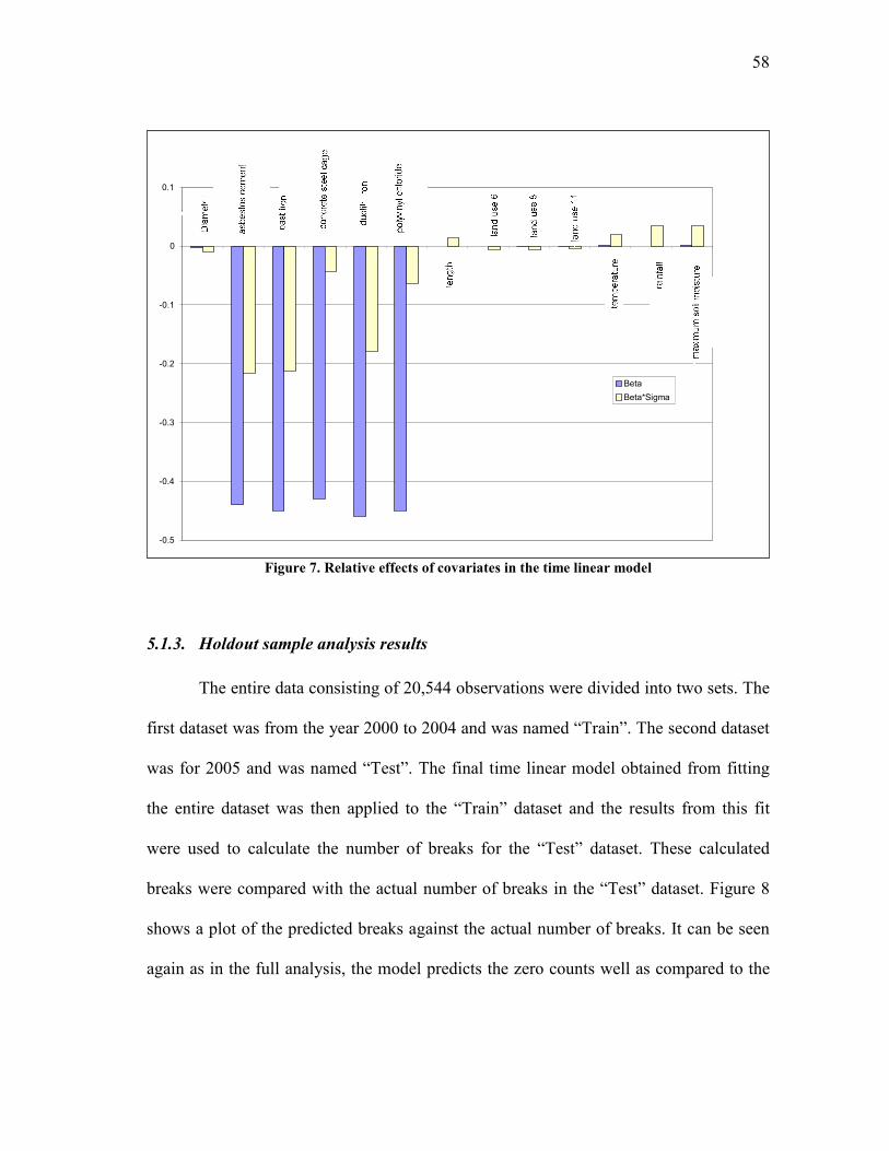
58
Figure 7. Relative effects of covariates in the time linear model
5.1.3. Holdout sample analysis results
The entire data consisting of 20,544 observations were divided into two sets. The
first dataset was from the year 2000 to 2004 and was named “Train”. The second dataset
was for 2005 and was named “Test”. The final time linear model obtained from fitting
the entire dataset was then applied to the “Train” dataset and the results from this fit
were used to calculate the number of breaks for the “Test” dataset. These calculated
breaks were compared with the actual number of breaks in the “Test” dataset. Figure 8
shows a plot of the predicted breaks against the actual number of breaks. It can be seen
again as in the full analysis, the model predicts the zero counts well as compared to the
-0.5
-0.4
-0.3
-0.2
-0.1
0
0.1
Beta Beta*Sigma

59
non zero counts. The MSE for the zero counts is 0.014 and for non-zero counts it is 1.12.
This is summarized in the table on page 74.
Figure 8. Holdout sample results for time linear model

60
5.1.4. Random holdout sample analysis
In this procedure, the complete data consisting of 20,544 observations was
divided randomly into five pairs, each pair consisting of a “Fit” dataset and a “Validate”
dataset. This was done by executing a MATLAB script. The script dropped 10% from
the full dataset randomly to give five different holdout samples. “Fit” was fit with the
statistical models described above and the results obtained were then used to calculate
the number of breaks in “Validate”. These calculated breaks were then compared with
the actual number of breaks in “Validate”. Figure 9 shows a plot of actual versus
predicted number of breaks for all the random holdout samples. The plots show that the
model behaves well when predicting zero breaks as compared to non-zero breaks. This
also reflects in the MSE values for random holdout sample analysis. They were 0.015,
0.014, 0.015, 0.015, and 0.015 for the zero counts for the five random holdouts.
Whereas, for the non-zero counts they were 0.96, 0.93, 0.85, 0.87, and 1. These are
summarized in the table on page 75.
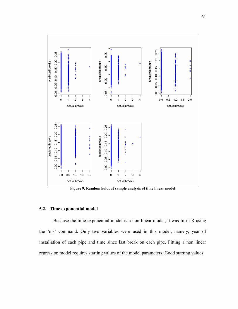
61
Figure 9. Random holdout sample analysis of time linear model
5.2. Time exponential model
Because the time exponential model is a non-linear model, it was fit in R using
the ‘nls’ command. Only two variables were used in this model, namely, year of
installation of each pipe and time since last break on each pipe. Fitting a non linear
regression model requires starting values of the model parameters. Good starting values

62
are those that are close to the true parameter values that minimize convergence
difficulties (Montgomery and Peck, 1992). A poor choice could result in convergence to
a local minimum of the function, and a suboptimal solution may be obtained. To obtain
good starting values for the model parameters, the solver add-in in Excel was first used
to find the set of parameter values that minimized the Sum of Squared Error (SSE).
These were then used as the starting values for the fitting done in R.
The fit results show that the number of breaks per time period for each pipe
increases with an increase in the time since the last break on the respective pipe. Time
since last break is statistically significant at a lower p-value than year of installation. An
examination of the predictive accuracy of the model through Figure 10 shows that the
model does better than the time linear model.
Figure 11 shows a QQ pot for the time exponential model. It is evident that the
residuals are not distributed normally.
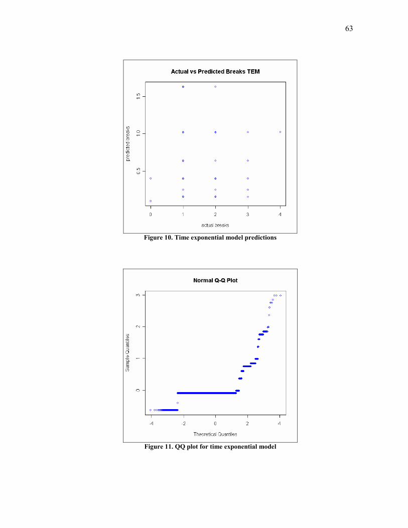
63
Figure 10. Time exponential model predictions
Figure 11. QQ plot for time exponential model

64
5.2.1. Holdout sample analysis results
Holdout sample analysis was performed in a similar fashion as in the time linear
model. Figure 12 shows a plot of the predicted breaks for the holdout sample. It can be
seen that the model predicts zero counts of breaks very well compared to the non-zero
counts. The Mean Square Error values computed for the zero counts and for the non-zero
counts of breaks for this model are 0.03 and 0.78 respectively. These are summarized in
the table on page 74.
Figure 12. Holdout sample analysis for time exponential model

65
5.2.2. Random holdout sample analysis
This analysis was performed exactly as done in the random holdout sample
analysis of time linear model. The same random holdouts were used. Figure 13 exhibits
predicted versus actual number of breaks for each pipe of the five “validate” samples.
Figure 13. Random holdout sample analysis for time exponential model

66
It can be seen that the model predicts zero counts of breaks better than the non-zero
counts. The MSE values for the five random holdouts were 0.003, 0, 0.0009, 0.003,
0.002 for zero counts of breaks and 1.146, 1.195, 0.664, 0.625, and 0.763 for non-zero
counts respectively. These Mean Square Error values are summarized in the table on
page 75.
5.3. Poisson generalized linear model
The table on page 68 gives the parameter significance results for ten different
Poisson GLMs together with the overall model fit results. One measure of the amount of
overdispersion in a data set is the deviance divided by the degrees of freedom, a quantity
known as the Pearson statistic. If this quantity is greater than 1, the data is overdispersed
relative to the Poisson model (Cameron and Trivedi 1998). For all of the models given in
Table 8, the Pearson statistic is less than 1, suggesting that overdispersion is not a
significant problem in this data set. The Poisson GLM is an appropriate model for this
data set.
There are a number of ways to assess the relative goodness of fit of different
Poisson GLMs. One of these is by comparing models based on the Akaike Information
Criterion (AIC) score of each model as explained in Section 4.5. Minimizing the AIC
yields a model that maximizes the log-likelihood with the minimum number of
parameters. Model 10 has all significant variables, and its AIC is reasonably close to that
of model 9 (model with the least AIC score). Model 10 is thus the preferred model.

67
5.3.1. Hypothesis Testing
A second approach for comparing Poisson GLMs is based on a likelihood ratio
test. The difference in deviance between two nested models (i.e., two models for which
the explanatory variables in one are a subset of the variables in the other) has
approximately a Chi-squared distribution with degrees of freedom equal to the difference
in degrees of freedom between the two models (see Cameron and Trivedi 1998).
Hypothesis tests were carried out to compare each successive model with the previous
model. The null hypothesis was that the new model and the previous old model have
deviances that are equivalent. With this criterion, it can be concluded that model 10 in
Table 8 provides a better fit than models 1-9 in Table 8 at a level of at least 0.05. This is
summarized in Table 7.
Among the models presented in Table 8, model 10 is thus the preferred model. It
cannot be shown to be inferior to the other models on the basis of a likelihood ratio test,
and it is the only model that includes all statistically significant variables. For Poisson
GLM model 10, the Transitional Areas land cover (Landuse 11) variable has the highest
p-value (0.036) followed by the Forest land cover (Landuse 8) variable (a p-value of
0.008) and Agricultural land cover (Landuse 6) variable (a p-value of 0.002). The other
covariates are significant at the 0.001 significance level.
The best fit regression equation for model 10 is given by equation (40) below where the
parameter definitions are the same as in the description of the data above.
4 3
3 3 4
log 6.84 (0.023)*( ) (0.12)*( ) (2.2 10 )*( ) (2.6 10 )( 6)
(3.2 10 )*( 8) (3.3 10 )*( 11) (0.0166)*( ) (2.65 10 )*( )
(0.012)*( )
DIA AC L LU
LU LU TEMP RAIN
SMAX
µ − −
− − −
=− − + + × − ×
− × − × + + ×
+
(40)

68
Table 7. Hypothesis tests for Poisson generalized linear model
MODEL NULL HYPOTHESIS p-value
1
H0: deviance(2) equivalent to deviance(1) 0.92
2
H0: deviance(3) equivalent to deviance(2) 0.841
3
H0: deviance(4) equivalent to deviance(3) 0.764
4
H0: deviance(5) equivalent to deviance(4) 0.708
5
H0: deviance(6) equivalent to deviance(5) 0.689
6
H0: deviance(7) equivalent to deviance(6) 0.603
7
H0: deviance(8) equivalent to deviance(7) 0.258
8
H0: deviance(9) equivalent to deviance(8) 0.186
9
H0: deviance(10) equivalent to deviance(9) 0.093
10

69
Table 8. Parameter significance results for Poisson generalized linear model
‘***’ signifies that the parameter is significant at p-values between 0 and 0.001, ‘**’ signifies that the parameter is significant at p-values between 0.001 and 0.01, ‘*’ signifies that the parameter is significant at p-values between 0.01 and 0.05, ‘.’ Signifies that the parameter is significant at p-values between 0.05 and 0.1, ‘N’ signifies that the variable was included in the model but was not significant, and a blank cell signifies that the parameter was not used in the model.
Model 1 2 3 4 5 6 7 8 9 10
Intercept N N N N N N N *** *** *** Diameter ** ** ** ** ** ** ** ** ** *** Asbestos cement
N ** ** ** ** ** ** ** ** **
Cast iron N N . . . N N N N Concrete steel cage
N N N N N
Ductile iron N Polyvinyl chloride
N
Length *** *** *** *** *** *** *** *** *** *** Year of installation
N N
Pressure N N N N N N N N Land use1 N N N N N N N Land use2 N N N N N N Land use3 N Land use4 N N N N . . N N N Land use5 N N N N Land use6 N N N N ** ** ** ** ** ** Land use7 N N N N . . N N Land use8 N . . . ** ** ** ** * ** Land use9 N N N N Land use10 N N N N N Land use11 N . . . ** ** * * * * Soil type1 N N N N N N N N Soil type2 N N N N N N N N
Soil type3 N N N N N N N N Soil type4 N N N N N N N N Soil type5 N N N N N N N Temperature ** ** ** ** ** ** *** *** *** *** Rainfall *** *** *** *** *** *** *** *** *** *** Maximum soil
moisture
*** *** *** *** *** *** *** *** *** ***
(max-min) soil
moisture
N N N N N N
Principal component
1
N N N
Principal component
2
N N N . . . . . .
Principal component
3
N N N
Residual Deviance
10343 10343 10344 10344 10344 10345 10347 10348 10353 10360
AIC 14961 14958 14954 14950 14946 14943 14941 14938 14931 14932 DF 20511 20513 20515 20517 20519 20521 20523 20525 20531 20534

70
Figure 14 shows a plot between actual breaks and predicted breaks for the
Poisson GLM. It is visually evident from Figure 10 and Figure 14 that the model does
not predict the zero and non-zero breaks as well as the time exponential model. Also
looking at Figure 4 and Figure 14, the Poisson GLM and the time linear model predict
the non-zero breaks in a similar fashion, but the time linear model predicts negative
values of the zero counts of breaks as opposed to the Poisson GLM.
Figure 14. Poisson generalized linear model predictions
5.3.2. Relative Effects of Variables
For any variable such as diameter for example, the relative rate of change in y
with respect to a change in jx can be written as
1 ( )
( )( )
j j
j
y
y x
µδ β
µ∂
= =∂
(41)

71
For categorical variables such as AC, CI, CSC, DI, and PVC that takes on values of 0
and 1, the interpretation of the derivative may be different, but the same formula is used
(Cameron and Trivedi, 1998). The units and variability of each covariate jx are different.
Hence the meaning of a unit change is different (Liu et al., 2005). To take into account
this variability, the product of jβ and jσ is considered.
j j jσδ β σ= (42)
The parameters jδ and jσ
δ give an indication of the impacts of each covariate on the
expected number of breaks and their relative importance (Cameron and Trivedi, 1998).
Figure 15 displays a bar chart indicating the magnitude of the estimates of each
covariate and the magnitude of the product of the estimate and the standard deviation for
each covariate. It can be seen that the pipe material Asbestos Cement has the largest
positive impact followed by temperature and maximum soil moisture on the predicted
number of breaks, whereas diameter has the most negative impact on the predicted
number of breaks. Based on these observations, it can be said that Asbestos Cement is
not a good material for manufacturing pipes for water distribution systems, as it has a
high incidence of breakage rate. Temperature, rainfall and soil moisture have high
variability. Thus their values can vary from one extreme to the other. This is likely to
affect pipe breaks due to the fact that the area where this water utility is located has
predominantly clay soils which shrink and swell. On the other hand, with decrease in
diameter of pipes, the breakage rate increases.
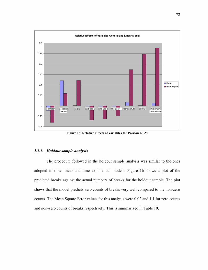
72
Relative Effects of Variables Generalized Linear Model
-0.1
-0.05
0
0.05
0.1
0.15
0.2
0.25
0.3
diameter asbestos
cement
length land use 6 land use 8 land use 11 temperature rainfall maximum
soil moisture
Beta
Beta*Sigma
Figure 15. Relative effects of variables for Poisson GLM
5.3.3. Holdout sample analysis
The procedure followed in the holdout sample analysis was similar to the ones
adopted in time linear and time exponential models. Figure 16 shows a plot of the
predicted breaks against the actual numbers of breaks for the holdout sample. The plot
shows that the model predicts zero counts of breaks very well compared to the non-zero
counts. The Mean Square Error values for this analysis were 0.02 and 1.1 for zero counts
and non-zero counts of breaks respectively. This is summarized in Table 10.
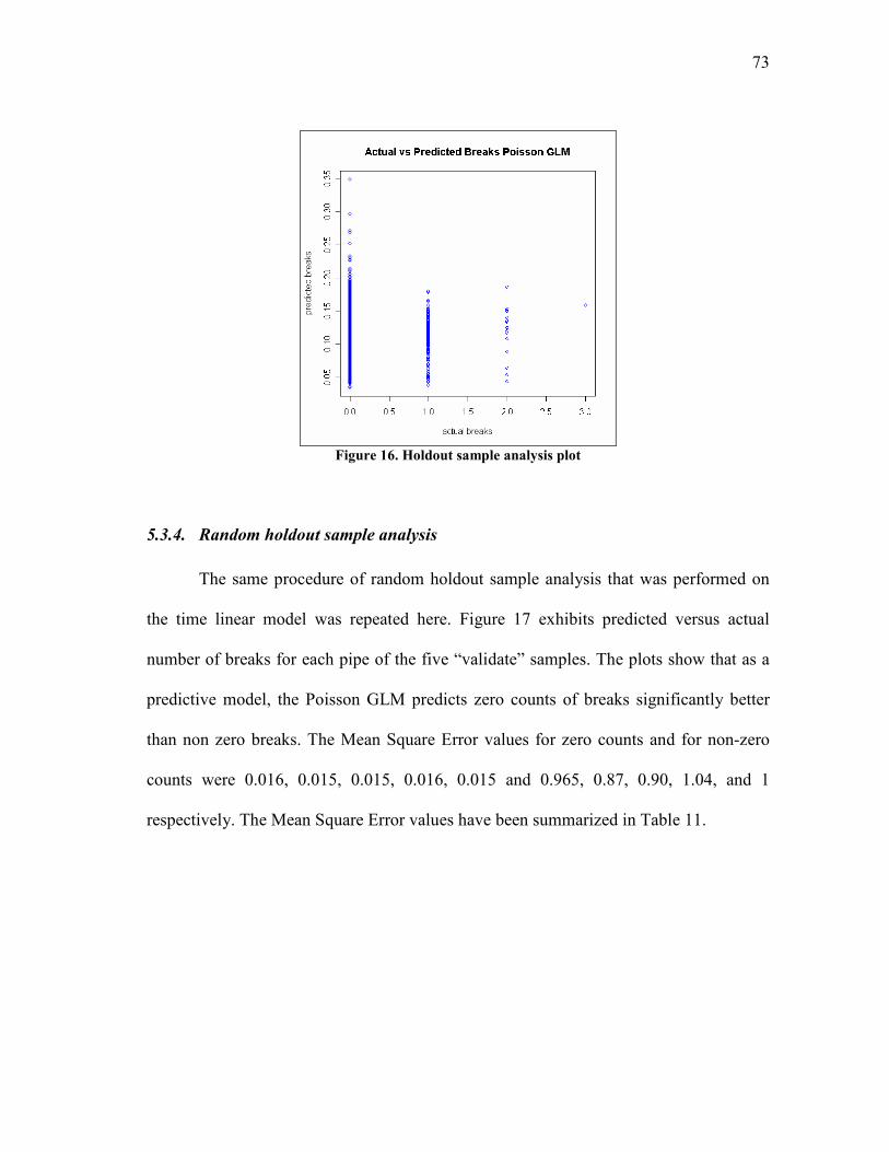
73
Figure 16. Holdout sample analysis plot
5.3.4. Random holdout sample analysis
The same procedure of random holdout sample analysis that was performed on
the time linear model was repeated here. Figure 17 exhibits predicted versus actual
number of breaks for each pipe of the five “validate” samples. The plots show that as a
predictive model, the Poisson GLM predicts zero counts of breaks significantly better
than non zero breaks. The Mean Square Error values for zero counts and for non-zero
counts were 0.016, 0.015, 0.015, 0.016, 0.015 and 0.965, 0.87, 0.90, 1.04, and 1
respectively. The Mean Square Error values have been summarized in Table 11.

74
Figure 17. Random holdout sample analysis of Poisson GLM
Table 9 summarizes the goodness of fit statistics for the time linear, time
exponential, and Poisson GLM models. Table 10 and 11 summarize the Mean Square
Errors (MSE) and the ratio of Root Mean Square Error (RMSE) to the average number
of breaks in the system for the TLM, TEM, and Poisson GLM models respectively for
holdout sample analysis and random holdout sample analysis. As far as Deviance and
AIC are concerned, the model with the least values of these statistics is considered a

75
good model. On the other hand, the model with the highest log-likelihood is considered a
good model. Table 9 suggests that the time exponential model is the best among the
three models.
Table 9. Goodness of fit statistics for all models
Model Deviance Log-Likelihood Degrees of Freedom
AIC
TLM 2405.45 -7118.96 20530 14267.91 TEM 1141.57 -537.09 20541 1066.18
Poisson GLM 10360 -7456.03 20534 14932
The Mean Square Errors for all three models were computed separately for zero
count and non zero count breaks. This was done because the data consists of nearly 90
percent pipe segments with zero breaks. Table 10 shows that all three models predict
zero counts reasonably well and are nearly equivalent. With respect to non-zero counts,
the TEM does the best.
Table 10. Mean square error for holdout sample analysis of all models
Table 11 displays the minimum, mean and maximum of Mean Square Errors as
well as the ratio of Root Mean Square Error to the average number of breaks for all the
three models. This ratio explains the relation between the root mean square error and the
Mean Square Error RMSE/Average no. of
breaks Model
For Zeros For Non-zeros For Zeros For Non-zeros
TLM 0.014 1.12 0.986 8.82 TEM 0.03 0.78 1.443 7.36
Poisson GLM 0.02 1.1 1.178 8.74

76
average number of breaks. Ideally this ratio should be close to zero. For example, in case
of the time exponential model, the root mean square error is 1.44 times the average
number of breaks for zeros and 7.36 times the average number of breaks for non-zeros.
Unlike the holdout sample analysis, the TEM is the best model for predicting zero counts
as well as non-zero counts of breaks.
In general, all the models that were applied in this research are not good
predictors of non-zero counts of breaks. A possible reason for this could be due to the
fact that the data is heavily zero inflated. Usually, when there a lot of zeros in the
response variable, it is advisable to try zero inflated models. The most common zero
inflated models are the Zero Inflated Poisson (ZIP) and the Zero Inflated Negative
Binomial (ZINB) models. To deal with the inability of the three models to predict non-
zeros well, it was decided to try the Logistic GLM. Instead of predicting actual counts of
breaks, this model predicts the probability of having breaks on any particular pipe.
Table 11. Mean square error for random holdout sample analysis of all models
Model
Mean Square Error TLM TEM Poisson GLM
Min 0.0148 1.67x10⁻⁷ 0.015
Mean 0.0152 0.0017 0.0155 For Zeros
Max 0.0154 0.003 0.016 Min 0.847 0.625 0.87 Mean 0.924 0.878 0.955 For Non Zeros
max 1 1.195 1.04
Root Mean Square
Error/Average number
of breaks
For Zeros 1.02 0.34 1.02 For Non-zeros 8.01 7.8 8.14
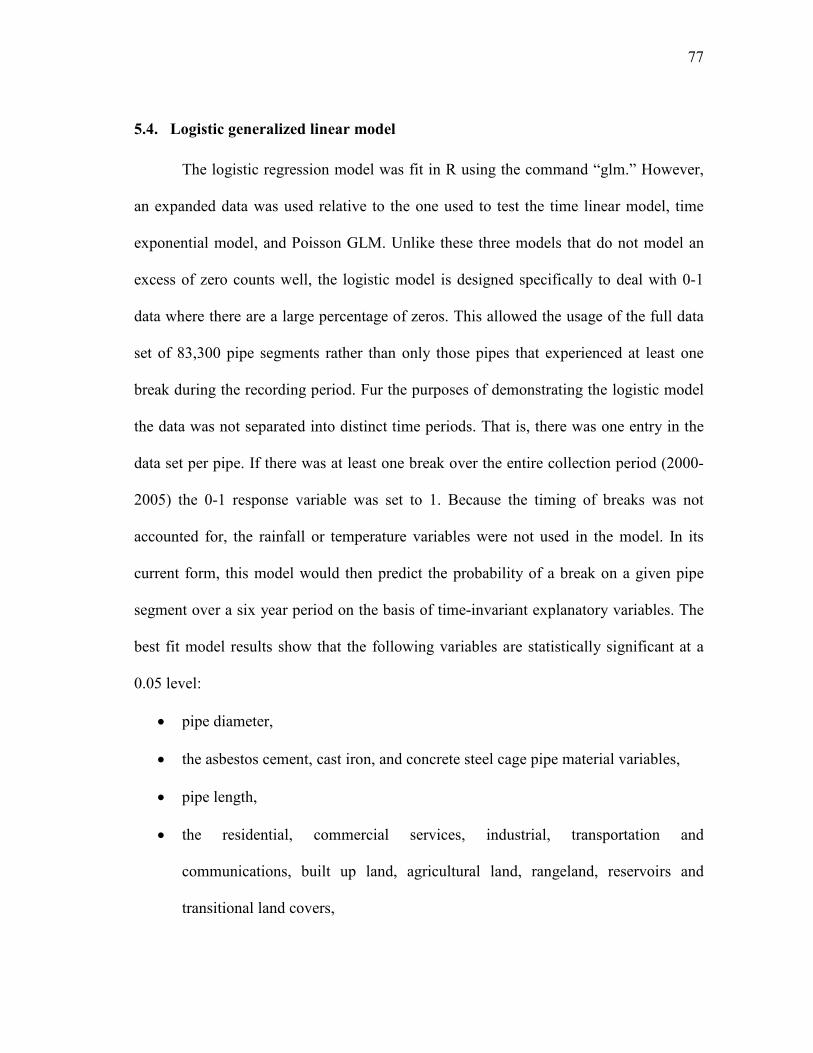
77
5.4. Logistic generalized linear model
The logistic regression model was fit in R using the command “glm.” However,
an expanded data was used relative to the one used to test the time linear model, time
exponential model, and Poisson GLM. Unlike these three models that do not model an
excess of zero counts well, the logistic model is designed specifically to deal with 0-1
data where there are a large percentage of zeros. This allowed the usage of the full data
set of 83,300 pipe segments rather than only those pipes that experienced at least one
break during the recording period. Fur the purposes of demonstrating the logistic model
the data was not separated into distinct time periods. That is, there was one entry in the
data set per pipe. If there was at least one break over the entire collection period (2000-
2005) the 0-1 response variable was set to 1. Because the timing of breaks was not
accounted for, the rainfall or temperature variables were not used in the model. In its
current form, this model would then predict the probability of a break on a given pipe
segment over a six year period on the basis of time-invariant explanatory variables. The
best fit model results show that the following variables are statistically significant at a
0.05 level:
• pipe diameter,
• the asbestos cement, cast iron, and concrete steel cage pipe material variables,
• pipe length,
• the residential, commercial services, industrial, transportation and
communications, built up land, agricultural land, rangeland, reservoirs and
transitional land covers,

78
• soil types variables for the 0-15 percent clay, 35-55 percent clay categories, and
principal component 1.
The ductile iron variable, the year of installation, pressure, the forest land cover
(LU8), the land cover of bare exposed rock (land use 10), soils with clay percentages
between 15-35, 55-65, and 65-80 were removed from the model since they did not turn
out to be significant in the models tried before obtaining the final model. The parameter
significance results along with the overall model fit results are listed in Table 12.
Equation (43) shows the final model with the parameter estimates.
3
( )logit[ ( )] log 5.82 (0.12)*( ) (1.21)*( ) (1.48)*( ) (1.84)*( )
1- ( )
(1.6 10 )*( ) (0.02)*( 1) (0.02)*( 2) (0.02)*( 3) (0.02)*( 4) 0.02*( 5)
(0.01)*( 6) (0.02)*( 7) (0.02)*(
P xP x DIA AC CI CSC
P x
L LU LU LU LU LU
LU LU
−
= = − − + + +
+ × + + + + +
+ + + 9) (0.02)*( 11) (0.01)*( 1) 0.005*( 3)
(0.02)*( 1)
LU LU ST ST
PC
+ − −
−
(43)
The deviance for this model was 20,559 for 83,282 degrees of freedom and the AIC was
20,595 for the same number of degrees of freedom. The low deviance/degrees of
freedom ratio combined with the AIC value substantially below the degrees of freedom
suggest that this model fits the data reasonably well. Also, a hypothesis test done to
compare the deviances of the final model to that of the null model gives a p-value of 1.
The high p-value shows that the final model is a good model for this dataset.
The parameter values suggest that larger pipes are less likely to experience
breaks. The fact that all of the regression parameters for the included pipe materials are
positive, suggests that these material types are more likely to experience breaks than
PVC pipe, the omitted material type. Furthermore, concrete steel cage (CSC) and cast
iron (CI) pipes are likely to have the highest breakage risk from among all pipe types, all

79
other variables being equal. Conclusions such as this can help guide pipe inspection
decisions. More specific guidance can come from examining the predicted probabilities
of breaks for each pipe and coupling this with an estimate of the severity of not catching
a break on a given pipe.
5.4.1. Random holdout sample analysis
The large dataset consisting of 83,300 pipe segments was divided into five
different pairs, each pair consisting of a “fit” dataset that was fit with the Logistic GLM
and a “validate” dataset which was used to validate the model i.e. the dataset for which
predictions were done using the model. The Mean Square Errors for all five samples
were calculated separately for zeros and ones, and the mean of all these MSEs turned out
to be 0.25. The ratio of Root Mean Square Error to the average number of breaks was
found to be 4.17.

80
Table 12. Parameter significance results for logistic generalized linear model
Model 1 2 3 4 5 6 7 8 9 10
Intercept N N N . . . . *** *** ***
Diameter *** *** *** *** *** *** *** *** *** ***
Asbestos cement
N *** *** *** *** *** *** *** *** ***
Cast iron N *** *** *** *** *** *** *** *** ***
Concrete steel cage
N *** *** *** *** *** *** *** *** ***
Ductile iron N . . . . .
Steel N * * * * * N N N
Length *** *** *** *** *** *** *** *** *** ***
Year of installation
N N
Pressure N N
Land use1 . . . . . . . *** *** ***
Land use2 . . . . . . . *** *** ***
Land use3 . . . . . . . *** ***
Land use4 . . . . . . . *** *** ***
Land use5 . . . . . . . *** *** ***
Land use6 . . . . . . . *** *** ***
Land use7 . . . . . . . *** *** ***
Land use8 . . . . . . .
Land use9 . . . . . . . * *** *
Land use10 . . . . . . . N
Land use11 . . . . . . . *** *** ***
Soil type1 N N N *** *** *** *** *** *** ***
Soil type2 N N N
Soil type3 N N N *** *** *** *** *** *** ***
Soil type4 N N N
Soil type5 N N N N
Principal component 1
N ** ** ** ** ** ** ** ** **
Principal component 2
N N N N N
Principal component 3
N
Residual Deviance
20541 20544 20544 20545 20546 20549 20552 20555 20557 20559
AIC 20601 20600 20596 20593 20592 20593 20594 20595 20595 20595
DF 83270 83272 83274 83276 83277 83278 83279 83280 83281 83282
‘***’ signifies that the parameter is significant at p-values between 0 and 0.001, ‘**’ signifies that the parameter is significant at p-values between 0.001 and 0.01, ‘*’ signifies that the parameter is significant at p-values between 0.01 and 0.05, ‘.’ Signifies that the parameter is significant at p-values between 0.05 and 0.1, ‘N’ signifies that the variable was included in the model but was not significant, and a blank cell signifies that the parameter was not used in the model.

81
5.5. Comparison of Poisson GLM and Logistic GLM
From the predicted breaks obtained by applying the Poisson GLM to the smaller
dataset of 20,796 observations, the probability of having one or more breaks for the zero
counts of breaks and the non-zero counts of breaks were obtained using equation (20).
Histograms of these predicted probabilities are shown in Figure 18. To compare the
Poisson GLM and the Logistic GLM, the Logistic GLM was applied to the smaller
dataset. From the predicted probabilities that were calculated, histograms were plotted
separately for the 0 variable and the 1 variable for probability of having one or more
than one break. These are shown in Figure 19. In each of these figures, the histogram on
the left of the figure is for the zero counts and the one on the right is for the non-zero
counts. It can be clearly seen from the two figures that the Poisson GLM and Logistic
GLM are equivalent in predicting the zero counts and the non-zero counts for the same
set of pipes.

82
0 0.1 0.2 0.3 0.40
1000
2000
3000
4000
5000
6000
7000
8000
9000
Probability of having one or more breaks
For zeros
0 0.2 0.4 0.6 0.80
100
200
300
400
500
600
700
800
Probability of having one or more breaks
For non-zeros
Figure 18. Probability of having one or more breaks for Poisson generalized linear model
Figure 19. Probability of having no breaks or more than one break for logistic generalized linear
model
0.05 0.1 0.15 0.2 0.250
2000
4000
6000
8000
10000
12000
Probability of having one or more breaks 0.05 0.1 0.15 0.2 0.250
200
400
600
800
1000
1200
1400
Probability of having one or more breaks
For zeros For ones

83
5.6. Summary
In this research, four different models namely, the time linear model, the time
exponential model, the Poisson Generalized Linear Model, and the Logistic Generalized
Linear Model were used. The smaller dataset consisting of 20,796 observations were fit
with the time linear, time exponential, and the Poisson GLM, whereas the larger dataset
consisting of 83,300 observations were fit with the Logistic GLM.
The results from fitting the time linear model to the data show that the model is
not a good model for modeling water distribution system reliability. The R-squared
value for this model is very low i.e. 0.117. This clearly shows that the relationship
between the predicted breaks and the actual breaks is not linear. The time exponential
model behaves better than the time linear model in fitting this data. The fit results
indicate that the number of breaks per time period for each pipe increases with an
increase in the time since the last break on the respective pipe. For the Poisson GLM the
Pearson statistic is less than 1 indicating that there is no overdispersion in the data. The
model appears to be modeling the number of breaks pretty similar to the time linear
model.
A comparison of the goodness of fit between the time linear, time exponential
and Poisson GLM models shows that the AIC, deviance and the log-likelihood for the
time exponential model are the best according to the criteria mentioned in Section 4.5.
As far as predictive ability is concerned, again the time exponential model does well in
modeling the zero counts as well as the non-zero counts of breaks.

84
For the logistic GLM, the low deviance/degrees of freedom ratio combined with
the AIC value substantially below the degrees of freedom suggest that this model fits the
data reasonably well. Also, a hypothesis testing done to compare the deviances of the
final model to that of the null model gives a p-value of 1. The high p-value shows that
the final model obtained after going through the stepwise regression procedure is a good
model for this dataset. A random holdout sample analysis carried out to check the
predictive accuracy of the model in estimating the probability of future breaks gives an
MSE of 0.25. The logistic GLM is a regression model that has been specifically
designed to handle excess amount of zeros in the data and it does this job successfully in
this research by giving a low MSE value for no break pipes.
A Logistic GLM was also fit to the smaller dataset. The overall fit results give an
AIC value of 14,097 and a deviance of 14,061. The log-likelihood for this model is -
7,030.34. Comparing these values to those of the time linear, time exponential and the
Poisson GLM (Table 9), it can be observed that the Logistic GLM has lower AIC and
higher log-likelihood than the time linear and the Poisson GLM, but it has higher AIC,
deviance and lower log-likelihood than the time exponential model. The logistic GLM
and the Poisson GLM predict the zero counts of breaks equivalently but the logistic
GLM does well in predicting the non-zero counts of breaks.

85
6. DISCUSSION
The present state of deterioration in water distribution systems gives rise to
questions regarding optimal repair, replacement and rehabilitation strategies that need to
be implemented. The heavy presence of zero counts of breaks in the water distribution
system data used in this research indicates that the system has been well maintained and
is pretty robust. However, the results from this research show that the water utility
cannot relax on this issue. The water utility managers still have to be on their toes to
ensure that in the future their distribution system remains robust.
6.1. Applications of the logistic GLM
One could envision water utilities assigning ranks to all the pipes in their
distribution systems based on probabilities predicted by using models like the Logistic
GLM. Then a plot such as the one shown in Figure 20 could be made. In this plot, the X-
axis represents the ranking of pipes based on predicted probabilities obtained by
applying the above model and the Y-axis represents the fraction of pipes at or above the
rank that had a break. Since zeros and ones were being predicted, there were bound to be
a lot of pipes with the same predicted probabilities. Thus these pipes were assigned the
same ranks. After manually counting the number of pipes it can be deduced that if the
first 30 ranked pipes are observed, only about 100 pipes need to be inspected. The
probability of finding a break per pipe would be nearly 35%. However, if the utility
decides to inspect 100 pipes at random from the 83,300 pipes, then the probability of
finding a break per pipe would be about 5%. By conducting this random inspection, the

86
utilities would be wasting their precious time, manpower and monetary resources. A
water utility would thus concentrate their resources on inspecting those first 30 ranked
pipes. Thus a plot such as Figure 20 could be really beneficial to water utilities trying to
conserve their precious time and monetary resources.
0 10 20 30 40 50 60 70 80 90 1000
0.1
0.2
0.3
0.4
0.5
0.6
0.7
0.8
0.9
1
Ranks based on predicted probability of breaks
Fraction of pipes at or above the rank that had a break
Figure 20. Plot of ranking of pipes against fraction of pipes at or above the rank that had a break
6.2. Applications to other systems
The results from these models could be used for modeling reliability of other
water distribution systems too. However, care will have to be taken in applying these
models to other water distribution systems, especially those in other regions where the
local ground conditions and meteorological conditions could differ substantially from

87
that in the area where this water utility is located. Similar models could be fit using data
from a different region if such data becomes available. Extension of the proposed
models to analyze failure records on sewers, oil and gas pipelines, depending on the
availability of data, could generate useful insights about the behavior of such systems.
6.3. Limitations in analysis
This research has been successful in modeling water distribution system
reliability. However, there are a few limitations that need to be addressed to make the
modeling more robust.
The biggest limitation is the size of the data. The data used is heavily left
censored. This limits the use of models such as Proportional Hazards model and
Accelerated Lifetime model which are particularly designed for modeling failure of
individual or group elements in a system. Even for the models used in this research data
worth 10 to 15 years at least would have comparatively provided a lot of insight into the
system.
Additional covariates could have made the models more accurate. In the models,
external corrosion was considered. Internal corrosion due to presence of different
compounds in water also plays a significant role in deteriorating pipelines in water
distribution systems. However, the difficulty of obtaining this data and lack of time
forced the use of external corrosion only. The pH of soil in which the pipes are buried,
the redox potential and saturated soil resistivity are important parameters that could give
an idea about the chemical properties of soil. Traffic loading, data on construction

88
activities in the area and number of repairs carried out up to the time under consideration
are other factors that could have provided more insight into the system.
Finally, the use of other models such as negative binomial GLM, negative
binomial GAM and Multivariate Additive Regression Splines (MARS) probably could
have more accurately modeled the system. However, lack of time prevented the
application of these models.
6.4. Suggestions for future research
It is evident from the dataset there are about 90% zero counts of breaks. As
mentioned in Section 5, zero inflated models are specifically designed to model zero
values in the dependent variable. A future endeavor in this research could be to try
applying the Zero inflated Poisson (ZIP) model to the dataset of 20,796 observations.
The results from this research could be further used in calculating maintenance
costs (including repair and replacement costs). From these parameters optimal
replacement time of pipes could be calculated. Also decisions on whether to repair or
replace an affected pipeline can be taken by using the results obtained. For example,
Hong et al. (2006) developed and demonstrated an approach for the prioritization of
replacement or rehabilitation activities associated with buried pipe networks. Their
approach was based on the minimization of the expected annual average cost associated
with the planning period of pipelines. Kleiner et al. (1998) used the time exponential
model of Shamir and Howard (1979) to develop a cost model to calculate the present
value of breakage repairs for the years elapsed from the present to the year of
89
rehabilitation using the cost of single breakage repair. The models used in this research
could be used to develop such cost models.
Kleiner et al. (1998) used the equation developed by Sharp and Walski (1988) to
model the effect that aging has on the carrying capacity of pipes in the distribution
network. They determined this capacity separately for pipelines before rehabilitation and
after rehabilitation. Thus the predicted probabilities of failure could be combined with a
numerical hydraulic model of the water distribution system to examine the consequences
of a break in terms of flow and pressure reductions in areas at various distances from the
break. Sometimes water utilities have to make decisions on whether to repair or replace
an affected pipeline. The results from statistical models such as those used in this
research could be extremely useful in developing models to facilitate such decisions.
90
7. CONCLUSION
In this research, the time linear, time exponential and Poisson GLM models were
reviewed based on pipe break data from 2000-2005 from a water utility company serving
a large city in Texas. The tests of these models suggest that the time exponential model
and the Poisson GLM are reasonably accurate predictive models for pipe breakage risk,
especially zero counts of breaks. The time linear model gives a very low R-squared
value and it predicts negative values for the zero counts of breaks. Hence it is not a good
model for this dataset. A comparison of the three models based on AIC, deviance and
log-likelihood shows that the time exponential model turns out to be the best model.
A model may be very good statistically, but applying it for predicting future
events is important from public safety and policy making point of view. The holdout
sample analysis and the random holdout sample analysis were used to test the predictive
accuracy of these models. The parameter of MSE was used to compare the predictive
ability of these models. Based on this, the time exponential model behaves better than
the time linear model and the Poisson GLM. Based on the results obtained from the time
linear model and the Poisson generalized linear model, the diameter of pipes, the
material asbestos cement, land cover variables of forest landuse, agricultural landuse and
transitional land use, and meteorological variables like temperature, rainfall and soil
moisture appear to be contributing the most to causing the breaks in the system. From
the results obtained after fitting the time exponential model to the data, the number of
breaks appears to be increasing with increase in time since last break.

91
The logistic GLM was applied to the larger dataset consisting of 83,300
observations. The ratio of deviance to degrees of freedom was small and the AIC value
was also considerably small. This shows that the model fit the data reasonably well. The
logistic GLM was also applied to the smaller dataset of 20,796 observations and
compared with the other three models. The results show that the AIC, deviance and log-
likelihood of this model were better compared to the time linear model and the Poisson
GLM. However, they were not so good compared to those of the time exponential
model. A comparison between the Poisson GLM and the logistic GLM based on MSE
shows that the two models are equivalent in predicting the zero counts of breaks but the
logistic GLM does well in predicting the non-zero counts of breaks.
92
REFERENCES
Agresti, A. (2002). Categorical Data Analysis, 2nd Ed. Hoboken, NJ: Wiley-
Interscience.
Akaike, H. (1974). “A New Look at the Statistical Model Identification,” IEEE
Transactions on Automatic Control, AC-19 (6) 716-723.
Andreou, S.A., (1986). “Predictive models for pipe break failures and their implications
on maintenance planning strategies for water distribution systems,” unpublished PhD
Thesis, Department of Civil Engineering, Massachusetts Institute of Technology,
Cambridge, MA, 1985.
Andreou, S. A., Marks, D.H., and Clark, R. M. (1987). “A new methodology for
modeling break failure patterns in deteriorating water distribution systems:
Applications.” Advance in Water Resources, 10, 11-20.
Baracos, A., Hurst, W.D., and Legget, R.F. (1955). “Effects of physical environment on
cast iron pipe,” Journal of American Water Works Association, 47(12), 1195-1206.
Belsley, D. A., Kuh, E. and Welsch, R. E. (1980) Regression Diagnostics. New York:
Wiley.
Cameron, A.C., and Trivedi, P.K. (1998). Regression Analysis of Count Data,
Econometric Society Monographs No. 30, Cambridge, UK: Cambridge University Press.
Cangelosi, R. and Goriely, A. (2007). “Component retention in principal component
analysis with application to cDNA microarray data,” Biology Direct, 2(2), 1-18.

93
Clark, C. M., (1971). “Expansive-soil effect on buried pipe.” Journal of American Water
Works Association, 63, 424-427.
Clark, R. M., Stafford, C. L., and Goodrich, J. A. (1982). “Water distribution systems: A
spatial and cost evaluation.” Journal of Water Resources Planning and Management,
108(3), 243-256.
Clark, R. M., Grayman, W. M., and Males, R.M. (1988). “Contaminant propagation in
distribution systems.” Journal of Environmental Engineering, 114(2), 929-943.
Cox, D. R. (1972). “Regression models and life tables,” Journal of Royal Statistical
Society, 34(B), 187-220.
Cox, D. R., and Oakes, D., (1984). Analysis of Survival Data. Chapman and Hall,
London, England.
Guikema, S.D., Davidson, R.A. and Liu, H. (2006). “Statistical Models of the Effects of
Tree Trimming on Power System Outages,” IEEE Transactions on Power Delivery, 21
(3), 1549-1557.
Guikema, S.D. and Davidson, R.A. (2006). “Modeling Critical Infrastructure Reliability
with Generalized Linear Mixed Models,” Probabilistic Safety Assessment and
Management (PSAM) 8, New Orleans, May 2006.
Hong, H., Allouche, E., and Trivedi, M. (2006).”Optimal Scheduling of Replacement
and Rehabilitation of Water Distribution Systems,” Journal of Infrastructure Systems,
12(3), 184-191.
94
Hotelling, H. (1933). “Analysis of a complex of statistical variables into principal
components.” Journal of Educational Psychology, 24:417-441, 498-520.
Hudak, P., Sadler, B., and Hunter, B. (1998). “Analyzing underground water-pipe breaks
in residual soils,” Water Engineering Management, 145(12), 15-20.
Jacobs, P., and Karney, B. “GIS development with application to cast iron water main
breakage rate.” 2nd Int. Conf. on Water Pipeline Systems, BHR Group Ltd., Edinburgh,
Scotland.
Kettler, A.J., Goulter, I.C. (1985). “An analysis of pipe breakage in urban water
distribution networks,” Canadian Journal of Civil Engineering, 12, 286-293.
Kiefner, J.F., and Vieth, P.H. (1989). “Project PR-3-805: A modified criterion for
evaluating the remaining strength of corroded pipe,” Pipeline Corrosion Supervisory
Committee of the Pipeline Research Committee of the American Gas Association.
Kim, S., Gruttola, V.D. (1999). “Strategies for Cohort Sampling under the Cox
Proportional Hazards Model, Application to an AIDS Clinical Trial,” Lifetime Data
Analysis, 5(2), 149-172.
Kleiner, Y., Adams, B. J., and Rogers, J. S., (1998). “Long-term planning methodology
for water distribution system rehabilitation.” Water Resources Research, 34(8), 2039-
2051.
Kleiner, Y., and Rajani, B. B. (2000). “Considering Time-dependent Factors in the
Statistical Prediction of Water Main Breaks,” American Water Works Association
Infrastructure Conference Proceedings, Baltimore, MD.

95
Kleiner, Y., and Rajani, B. B. (2001). “Comprehensive review of structural deterioration
of water mains: Physical models,” Urban Water, 3(3), 177-190.
Kleiner, Y., and Rajani, B. B. (2001). “Comprehensive review of structural deterioration
of water mains: statistical models,” Urban Water, 3(3), 131-150.
Kumar, A., Meronyk, E., and Segan, E. (1984). “Development of concepts for corrosion
assessment and evaluation of underground pipelines,” U.S. Army Corps of Engineers,
Construction Engineering Research Laboratory, Technical Report CERL-TR-M-337, I1.
Marks, H. D., Andreou, S., Jeffrey L., Park, C., and Zaslavski, A. (1987). “Statistical
models for water main failures.” US Environmental Protection Agency (Co-operative
Agreement CR810558) M.I.T. Office of Sponsored Projects No. 94211, Boston,
Massachusetts.
Mavin, K., (1996). “Predicting the Failure Performance of Individual Water Mains,”
Research Report No. 114, Urban Water Research Association of Australia, ISBN
1876088176.
Mays, L. W., ed. (2000). Water distribution systems handbook. McGraw-Hill, New
York.
McMullen, L.D. (1982). “Advanced concepts in soil evaluation for exterior pipeline
corrosion,” In proceedings of the American Water Works Associationi Annual
Conference, Miami, FL.
Montgomery, D.C., Peck, E.A. (1992), Introduction to Linear Regression Analysis.
(Probability and Statistics Ser. No. 1346), 2nd Ed. Hoboken, John Wiley & Sons.

96
Morris, R (Jr.), (1967) “Principal causes and remedies of water main Breaks.” Journal of
American Water Works Association, 54 (7), 782-798.
National Oceanic & Atmospheric Administration. (2006). NOAA Satellite and
Information Service, National Climatic Data Center, Last accessed August 1, 2006
http://cdo.ncdc.noaa.gov/CDO/cdo.
O'Day, D. K., Fox, C. M., and Huguet, G. M. (1980). "Aging urban water systems: A
computerized case study." Public Works, 111(8), 61–64.
O’Day, D. K., and Staeheli, L. A. (1983). “Information Systems for Facility
Maintenance Decisions.” Report No. 2, Study conducted for the Urban Infrastructure
Network, The Urban Institute, contract No. 3264.
Rajani, B., Zhan, C., (1996). “On the Estimation of Frost Load,” Canadian Geotechnical
Journal, 33(4), 629-641.
Rajani, B., Zhan, C. and Kuraoka, S., (1996). “Pipe soil Interaction Analysis for Jointed
Water Mains,” Canadian Geotechnical Journal, 33(3), 393-404.
Schoenfeld, D. (1982). “Partial residuals for the proportional hazards regression model,”
Biometrika, 69(1), 239-241.
Scott, A. and Clarke, R. (2000). “Multivariate techniques,” Statistics in Ecotoxicology,
148-178, Wiley.
Shamir, U. and Howard, C.D.D., (1979). “An analytic approach to scheduling pipe
replacement.” Journal of American Water Works Association, 71(5), 248-258.
97
Sharp, W. W., and Walski, T. M. (1988). “Predicting Internal Roughness in Water
Mains.” Journal of American Water Works Association, 80(11), 34.
Stratus Consulting. (1998). “Infrastructure Needs for the Public Water Supply Sector.”
Report for American Water Works Association, Boulder, Colorado.
U.S. Army Corps of Engineers, New York District. (1980). “New York City Water
Supply Infrastructure Study.” Volume 1, Manhattan, NY.
U.S. Army Corps of Engineers. (1981). “Urban Water Study – Buffalo, New York,
“Volume 1, Final Report.
Walski, T. M., and Pellicia, A., (1982). “Economic Analysis of Water Main Breaks.”
Journal of American Water Works Association, 74(3), 140-147.
WebGIS. (2006). Geographic Information Systems Resource, Last accessed August 1,
2006. http://www.webgis.com/index.html.

98
APPENDIX A

99
LOADINGS FOR PRINCIPALCOMPONENTS
PC1 PC2 PC3 PC4 PC5 PC6
0.0079 0.9999 0.0078 0.0008 0 0
0.0005 0.0078 -0.9999 0.0108 0 0
0 0.0008 -0.0108 -0.9999 0 0
0 0 0 0 0 1
0 0 0 0 1 0
-1 0.0079 -0.0004 0 0 0

100
APPENDIX B
101
WORK DONE IN ArcGIS
The data for many of the covariates was provided in the form of layers. These
layers were part of shape files which spatially describe features such as points, lines and
polygons. Each of these features has attributes associated with them. A shape file can
have one or more layers forming a Geographic Information System (GIS). A GIS is a
system for capturing, storing, analyzing and managing data and related attributes that are
spatially referenced to the geographic location under consideration.
Using ArcMap (a part of ArcGIS), a platform for visualizing spatial data and
performing spatial analysis, the pipe network for this water utility was related to each
and every covariate used in the statistical analysis. The number of breaks on each pipe
segment being the dependent variable in this analysis, the first step was to relate the
break data to each pipe segment. A major hurdle in this process was the fact that some of
the breaks were slightly skewed from the pipes i.e. not lying exactly on the pipes,
probably because of measurement errors. This was taken care of by making buffers, 160
feet wide, around each pipe while spatially joining the breaks to the pipes using the
spatial join command in ArcMap. The covariates of pipe diameter, pipe length, pipe
materials, the year of installation of each pipe, and the time since last break on each pipe
were then extracted from the attributes of the pipe network layer.
The covariates of pressure, land use, soil type, and soil corrosivity were obtained
by doing GIS analysis as given below.

102
Pressure
The water distribution system under study is divided into 12 pressure zones and the data
was in the form of layers for each of these pressure zones. The pipes intersected by each
pressure zone were selected using the “Select by Location” tab in ArcMap and new
layers were made out of them. These new layers were then related spatially to the
pressure zones using the “Joins and Relates” tab and this way the pressure in each pipe
was obtained.
Land use
New layers were made using ArcMap in each of the eleven land covers obtained from
WebGIS. The pipe network was then clipped based on the above layers using the “Clip”
tool from the ArcToolbox. Then by using XtoolsPro (an extension for ArcGIS), the
lengths of each of the pipes in these clips were recalculated using the “Calculate Area,
Perimeter, Length, Area and Hectares” tab in “table Operations”. These lengths were
then converted to percentages of the overall pipe segment length.
Soil type
The soils were first grouped into five categories based on their clay content: 0-15 percent
clay, 15-35 percent clay, 35-55 percent clay, 55-65 percent clay and 65-80 percent clay.
Using ArcMap, layers were created for each category. Clips of the pipe network were
made using each of the category layers. The GIS toolbox XtoolsPro was used to
recalculate the length of each pipe within each soil group after clipping. These lengths
were then converted to percentages of the overall pipe segment length.
103
Soil Corrosivity
The soil corrosivity data obtained from SSURGO was overlaid on the pipe network and
clipping was done similarly to the one done in extracting soil type data. The length of
each pipe in each of the six soil corrosivities were then recalculated using XtoolsPro.
From this the percentage length of each pipe in each of the soil corrosivities were
calculated and these were then used in the statistical analysis.

104
VITA
Shridhar Yamijala received his Bachelor of Engineering degree in Civil
Engineering from Government College of Engineering, Pune in India in 2004. He started
his Master’s program at Texas A&M University, College Station in August 2005. His
research interests encompass risk and reliability analysis applied to infrastructure
systems. He worked as a Graduate Research Assistant for four semesters and graduated
with a Master of Science degree in Civil Engineering in August 2007.
Mr. Yamijala’s permanent address is B-1, 204, Hari Ganga, Opposite Phule
Nagar, Near Yerawada, Pune-411006, Maharashtra, India. His email address is