CoPS STYLE CGE MODELLING AND ANALYSIS

CoPS Working Paper No. G-264, November 2016

The Centre of Policy Studies (CoPS), incorporating the IMPACT project, is a research centre at Victoria University devoted to quantitative analysis of issues relevant to economic policy. Address: Centre of Policy Studies, Victoria University, PO Box 14428, Melbourne, Victoria, 8001 home page: www.vu.edu.au/CoPS/ email: copsinfo@vu.edu.au Telephone +61 3 9919 1877

Esmedekh Lkhanaajav

Centre of Policy Studies, Victoria University

ISSN 1 031 9034 ISBN 978-1-921654-72-5

Page | 1

CoPS style CGE Modelling and Analysis By

Esmedekh Lkhanaajav

Centre of Policy Studies,

Victoria University

Abstract

CoPS is a world leader in CGE modelling. This paper describes a brief history of CoPS style

of CGE modelling; from ORANI to new generation CoPS models, and discusses the

distinctive features of CoPS style models. In addition, it introduces solution methods,

notations, and tools that are used in CoPS style of CGE modelling and analysis.

Keywords: CGE modelling; CoPS style CGE modelling

JEL: C68, D58, B23

Page | 2

Contents 1. Introduction ........................................................................................................................ 3

2. A Brief History: From ORANI to new generation CoPS models ...................................... 7

2.1. ORANI ........................................................................................................................ 7

2.2. CoPS style dynamic models ...................................................................................... 11

2.3. CoPS style regional models....................................................................................... 12

2.4. Global Trade Analysis Project (GTAP) .................................................................... 13

2.5. New generation CoPS models ................................................................................... 14

3. A General form of CoPS style CGE model ...................................................................... 16

4. Solution methods .............................................................................................................. 17

4.1. Johansen solution procedure ..................................................................................... 18

4.2. Johansen/Euler solution procedure............................................................................ 19

4.3. Gragg’s method ......................................................................................................... 19

4.4. Richardson’s extrapolation ........................................................................................ 20

5. Standard notations and conventions ................................................................................. 20

6. Data requirement .............................................................................................................. 23

7. GEMPACK ....................................................................................................................... 23

8. Back-of-The-Envelope (BOTE) Analysis ........................................................................ 24

Page | 3

1. Introduction

Economics is the study of how economic agents – producers, investors, households,

foreigners and governments – make choices under conditions of scarcity, and of the results

and efficiency of those choices. In any economic system, scarce resources have to be

allocated among competing uses. These resources are allocated by the combined choices and

interactions of economic agents in an economy. Inevitably, the choices of economic agents

come down to the relative importance of competing uses, thereby creating trade-offs.

Economic theories postulate the optimising behaviour of economic agents under given

resource and technology constraints, with signalling from market prices. Households

maximise their utility subject to their budget constraints, and producers maximise their profits

subject to their production technology constraints. Prices, determined by market equilibria,

play a crucial role in resource allocation. Hence, the optimising behaviours of economic

agents are the means of introducing market or price mechanisms to the model (Dixon &

Rimmer 2002).

Interactions of agents and repercussions of episodes in an economy are capable of being

captured in an economy-wide general equilibrium framework. The theory of general

equilibrium analysis was pioneered by Walras (1877) and Edgeworth (1881). Leon Walras

provided the first general equilibrium description of a complex economic system with the

interactions of independent economic agents. Francis Edgeworth introduced the well-known

tool of general equilibrium analysis of exchange that is named after him – the Edgeworth

box. Major theoretical contributions related to the existence, uniqueness, stability and

optimality of general equilibria were made also by Kenneth Arrow, Gerard Debreu, Hiroshi

Atsumi, Hirofumi Uzawa and Michio Morishima from 1950 to the 1970s.

CGE modelling is an empirical approach of general equilibrium analysis. Since 1960, CGE

modelling has gradually replaced other economy-wide approaches such as input-output

modelling and economy-wide econometric modelling. It also became a dominant economy-

wide framework for policy analysis in 1990s, with a vast amount of literature concerning

various aspects and applications of CGE modelling (Dixon 2006; Dixon & Jorgenson 2013).

Dixon et al. (1992) described CGE modelling as an integration of a general equilibrium

theoretical structure, data about the economy of interest, and solution methods to solve the

models numerically. Dervis and Robinson (1982) identified CGE models as those that

‘postulate neo-classical production functions and price-responsive demand functions, linked

around an input-output matrix in a Walrasian general equilibrium model that endogenously

Page | 4

determines quantities and prices’. Shoven and Whalley (1992) defined CGE modelling as a

conversion of the Walrasian general equilibrium structure into realistic models of actual

economies by specifying production and demand parameters, and incorporating data

reflective of real economies. Dixon and Parmenter (1996) described the distinguishing

characteristics of CGE models as follows:

(i) CGE models are general since they include explicit specifications of the behaviour

of several economic agents/actors;

(ii) CGE models employ market equilibrium assumptions as they describe how

demand and supply decisions made by different economic agents determine the

prices of at least some commodities and factors that in turn ensure market

equilibria; and

(iii) CGE models are computable and produce numerical results.

CGE modelling can therefore be characterised by its applied nature and quantitative approach

in general equilibrium analysis. Applied general equilibrium (AGE) modelling is an

alternative term used to describe CGE modelling.

CGE models belong to the economy-wide class of models. Hence, they provide industry

disaggregation and the behaviours of economic agents in a quantitative description of the

whole economy. According to Dixon and Rimmer (2010), the original empirical economy-

wide model was Leontief’s input-output system (Leontief 1936). Leontief’s input-output

system portrays ‘both an entire economy and its fine structure by plotting the production of

each industry against its consumption from every other’ (Leontief 1951, p. 15). He provided a

tabular representation of the economy – the input-output tables. These tables show a detailed

disaggregation of the supply and use of inputs and outputs in the economy.

Leontief’s input-output system in matrix form can be shown as:

𝑋𝑋 = 𝐴𝐴𝑋𝑋 + 𝑌𝑌 (1)

where X is a vector of outputs; Y is a vector of final demands; and A is the input-output

coefficient matrix. In input-output modelling, the production of each commodity (the vector

X) satisfies the intermediate (the matrix AX) and final (the vector Y) demands with given

technology specified by the input-output coefficient matrix (A). Each input-output or

technical coefficient (𝑎𝑎𝑗𝑗𝑗𝑗) in matrix A defines the value of intermediate inputs that are

required by industry i from industry j to produce a unit of output in industry i (𝑎𝑎𝑗𝑗𝑗𝑗 = 𝑍𝑍𝑗𝑗𝑗𝑗/𝑋𝑋𝑗𝑗

Page | 5

where 𝑍𝑍𝑗𝑗𝑗𝑗 is the intermediate input sales from industry j to industry i). Input-output analysis,

as Leontief described (1951, p. 21), is ‘a method of analysis that takes advantage of the flow

of goods and services among the elements of the economy to bring a much detailed statistical

picture of the system into the range of manipulation by economic theory’. Input-output

modelling is still popular in applied economic research.

The next stage of economy-wide modelling was the programming model pioneered by

Sandee (1960). In his demonstration of the planning model for India, Sandee used a linear

programming method to maximise a welfare (material consumption) function, subject to

Leontief’s technology specification. Notable contributions to the programming models were

made by Manne (1963) and Evans (1972). H. D. Evans’ internationally acclaimed study of

protection in Australia was an important methodological contribution to the analysis of

protection and to the applied general equilibrium framework (Dixon & Butlin 1977).

Input-output and programming models could not provide underlying market mechanism of

interactions in the economy and lacked clear descriptions of the behaviour of individual

agents (Dixon & Rimmer 2010a). In these models, the economy is visualised as a single

agent (Dixon & Jorgenson 2013).

Lief Johansen (1960) advanced economy-wide modelling through the explicit identification

of behaviour by economic agents in his model of Norway’s economy. The publication of

Johansen’s book, ‘A Multi-sectoral Study of Economic Growth’, marked the birth of CGE

modelling (Dixon & Jorgenson 2013). In Johansen’s 22-sector model, households maximise

utility subject to their income constraints; industries choose primary and intermediate inputs

to minimise their costs of producing any given level of output, subject to their production

frontiers and the need to satisfy demands for their outputs; and investors allocate the

economy’s capital stock between industries to maximise their returns. The overall outcome

for the economy is determined by the actions of individual agents driven by the price

adjustment mechanism (invisible hand) that equalises demand and supply in various markets.

Dixon (2010a) reminds us that there was no single starting point for CGE modelling even

though Johansen was ‘the first one to plant a seed in what has now become the CGE forest’

(p. 5).

Herbert Scarf’s work (1967; Scarf & Hansen 1973) brought greater attention and enthusiasm

to CGE modelling. His students, John Whalley and John Shoven, further contributed to the

development of Scarf’s approach, which is also known as a combinatorial approach. Scarf’s

Page | 6

method, however, has been largely abandoned in favour of much simpler methods used by

other approaches (Dixon 2006).

Dale Jorgenson and his associates solved their CGE model by iterative methods

independently. They continue to make path-breaking contribution to CGE modelling through

theoretical and econometric innovations (Dixon & Jorgenson 2013; Dixon & Rimmer 2010a).

Irma Adelman, Sherman Robinson and their associates at the World Bank developed another

widely used CGE approach. The models developed using their framework belong to the

tradition of World Bank CGE modelling (Bandara 1991a). The Generalized Algebraic

Modelling System (GAMS) software (Brooke, Kendrick & Meeraus 1996) is used in their

Social Accounting Matrix based models.

Peter Dixon and his associates developed the Centre of Policy Studies (CoPS) approach,

adopting and extending Johansen strategies for computing, and for organising and

understanding results. In this sense, CoPS style modelling is directly descended from

Johansen. The influence of Johansen, combined with the institutional arrangements under

which CoPS style models have been developed, has given this form of modelling some

distinctive technical characteristics (Dixon, Koopman & Rimmer 2013). CoPS style models

are solved with the General Equilibrium Modelling Package (GEMPACK) software

(Harrison & Pearson 1996). The progress of CGE modelling software and the differences

among the main systems such as GEMPACK and the GAMS are detailed in Horridge et al.

(2012). CoPS style modelling is also known as ‘Australian style’ CGE modelling (Hertel,

2013).

Finally, Global Trade Analysis Project (GTAP), an exceptional venture and a collaborative

network of organisations and individuals, has emerged as a united force in CGE modelling,

bringing an explosion of interests in global environmental, trade, energy, land-use and many

other economic issues. Thomas Hertel and associates of the GTAP network have shaped the

development of CGE modelling into a new era since its inception in 1991. GTAP is now

recognised as a global brand of CGE modelling. Alan Powell, one of the founders of CoPS

style modelling, concludes ‘in the discipline of economics there has never been a research

oriented community as large or as enthusiastic as the associates of GTAP (Powell 2007).

GTAP modellers employ both GEMPACK and the GAMS.

Page | 7

2. A Brief History: From ORANI to new generation CoPS models

This section briefly describes the history of CoPS style of CGE modelling; from ORANI to

new generation CoPS models. ORANI and other CoPS style models can be readily identified

as belonging to the Johansen class of multi-sectoral models (Dixon, Koopman & Rimmer

2013; Dixon et al. 1982). Retaining the advantages of Johansen’s approach and combining

them with the institutional arrangements under which CoPS style models have been

developed, CoPS style modelling has become a well-recognised school of economic

modelling, thought and analysis with distinctive technical characteristics and a transferable

know-how.

2.1. ORANI

CoPS style models evolved from ORANI (Dixon et al. 1982). ORANI is a comparative static

model of the Australian economy. It was developed in the late 1970s in the framework of the

IMPACT project and has served as a foundation for CGE models of many countries. Its first

applications (Dixon et al. 1977; Dixon, Powell & Harrower 1977) brought a wide exposure in

the Australian economic policy debate (Powell & Snape 1992).

When summarising the most important developments in economic policy during 1967-1975,

Corden (1995) highlighted a long-run perspective of economic policy analysis. He wrote:

Thanks to Mr. Whitlam and the initiative of Mr. Rattigan, the Tariff Board was replaced by the Industries Assistance Commission (IAC), with Mr. Rattigan the chairman of the new IAC. Its mandate was much wider than that of the Tariff Board, and it was conceived on a much more ambitious scale. This was the beginning of an important and remarkable organisation, one which acquired a world reputation and which, through its careful empirical work and strong and consistent “economic rationalist” analysis, undoubtedly influenced informed thinking and policy-making in the broad area of industry assistance subsequently. There is really a remarkable contrast between the Tariff Board reports of the early sixties (and some of the reports reviewed in my 1967 lecture) which were empty of serious economic analysis, and the highly professional reports of the IAC, backed up with effective rate and subsidy equivalent measures and the use of general equilibrium modelling resulting from the IMPACT project (Anderson 2014, pp. 370-2).

In his most celebrated paper, ‘Gregory thesis’, Gregory (1976) foresaw the importance of the

IMPACT project and its models, and wrote:

Page | 8

To fully account for general equilibrium effects [of the rapid growth of mineral exports] would require a much more complex and computerised model such as the IMPACT model being developed by a number of Australian government departments (p. 75).

The abovementioned institutional arrangements have played an essential role for the

development of CoPS school of modelling. The Australian government-initiated IAC had set

up the IMPACT project under the direction of Powell, aimed at improving available policy

information systems for governments as well as for private and academic analysts. More

specifically, the IMPACT project was to build policy-oriented economy-wide models and to

organise training associated with these models (Dee 1994; Powell & Snape 1992).

The Productivity Commission (PC) acknowledged the origin of the IMPACT project as a

source of its strong analytical tradition in its 30th anniversary book titled ‘From industry

assistance to productivity: 30 years of the Commission’ as:

While the number of detailed tariff inquiries fell, their breadth and complexity increased, as did the depth of the analytical approaches employed. GA (Marshall) Rattigan, the first Chairman of the IAC, together with one of his senior advisors at the Commission, Bill Carmichael (later to become Chairman himself), realised the importance of developing quantitative models capable of analysing the economy-wide consequences of policy and policy changes for economic activity and employment, as well as for regions, sectors and individual industries. Effective rate calculations, although revealing, were not enough. Consequently, the IAC helped construct increasingly sophisticated quantitative economic models of the Australian economy (PC 2003a, pp. 4-5).

The integrity and vison of outstanding public servants (notably, A. Rattigan, W. Carmicheal

and B. Kelly), the insights and influences of Australian leading economists (notably, M.

Corden, B. Gregory and R. Snape) and the policy problem of much debated tariff were the

preconditions of the IMPACT project and its brainchild ORANI becoming influential in

Australian policy analysis immediately.

CGE modelling became influential, as Powell and Snape (1992) expressed, not just because

the tool had caught the imagination of some of Australia’s best economists (Dixon and

colleagues) but because it was the right tool for the policy problem at hand. They highlighted

the following conditions under which ORANI was developed; independence, full

documentation, and involvement of the policy clientele. Powell, in his foreword to ‘Global

Trade Analysis: Modelling and Applications’ (Hertel, 1997) , pointed out that the

Page | 9

replicability of an experiment is necessary for economics to earn its status as a science and

emphasised that ‘this can amount to a tall order’ in the case of CGE work (p. xiii). In fact,

ORANI showcases this ‘tall order’.

Dixon is the founder and leader of CoPS style modelling. After graduating with Honours in

Economics from Monash in 1967, he pursued his PhD at Harvard under Leontief’s

supervision. His PhD was awarded in 1972 by Harvard (Parmenter 2004). Titled ‘The Theory

of Joint Maximisation’, this thesis was subsequently published in the North Holland

Contributions to Economic Analysis series (Dixon 1975). His thesis made a number of

contributions to economic analysis, particularly to the literature on the computations of

numerical solution to general equilibrium models (Mackinnon 1976). Dixon introduced the

joint maximisation approach for the computation of equilibria and developed effective

algorithms, providing an alternative to Scarf’s combinatorial approach. The essence of the

theory of joint maximisation is ‘the notion that general equilibrium solutions may be found

by solving suitably chosen programming problems’ (Dixon 1975). Dixon acknowledged that

Evans’ 1968 PhD thesis inspired him to study for his PhD and named Evans as one of three

people who influenced him greatly. He was brought to the IMPACT project by Powell, one

of the founders for this school of modelling and also one of three people who influenced

Dixon greatly, to build an economy-wide model. Dixon integrated Armington’s imperfect

substitution specification (Armington 1969) with Leontief’s input-output model to build

ORANI. Originally, ORANI introduced a number of innovations such as: flexible closures;

multi-product industries and multi-industry products; the CRESH and CRETH substitution

possibilities; specifications of technical change and indirect taxes associated with every

input-output flow; explicit modelling of transport, wholesale and retail margins; and a

regional dimension (Dixon & Rimmer 2010a).

ORANI was initially built to analyse the impacts of high tariff, identifying the losers from

protection and quantifying their losses. ORANI showed how high tariffs caused high costs in

Australia and confirmed that cutting tariffs from the high levels in the 1970s would produce

overall benefits for Australia. ORANI simulations showed that cutting tariffs would increase

average wage rates – and hence, living standard – while not harming aggregate employment.

It would also stimulate export activity that would bring prosperity to regions like Western

Australia and Queensland (Dixon et al. 1977). Dixon (1978) reiterated his theory and

described how the theory of joint maximisation forms a basis for ORANI’s computational

technique by comparing his approach with that of Scarf.

Page | 10

ORANI was designed to provide results that would be persuasive to practical policy makers

rather than to academics, hence it encompassed considerable detail. The first version of

ORANI had 113 industries and a facility for generating results for Australia’s eight states and

territories. In addition to its industry and regional details, ORANI was equipped with detail in

other areas such as detailed specifications of margins that were normally ignored in academic

research (Dixon 2006).

Since 1977, ORANI has been used in numerous analyses and simulations on the effects of

mineral discoveries, major infrastructure projects, new technologies, mining booms and

busts, and the impacts of various government policies changes in policy instruments such as

import tariffs, other tax rates, public spending, interest rates, microeconomic and labour

market reform, as well as other environmental and legal regulations on the Australian

economy.

Reviews of several hundred published ORANI applications of early years in Australian

context can be found in Powell and Snape (1992) and Dee (1994).

ORANI, furthermore, has become the most diversely exported know-how or technology of

Australia, and has served as the foundation and starting template of models for many other

countries, including South Korea (Vincent 1982), New Zealand (Nana & Philpott 1983),

Papua New Guinea (Vincent 1991), the Philippines (Coxhead & Warr 1995; Coxhead, Warr

& Crawford 1991), South Africa (Horridge et al. 1995), Indonesia (Wittwer 1999), China

(Adams et al. 2000b) and many others. ORANI-Generic (Horridge 2000, 2014; Horridge,

Parmenter & Pearson 1998) is a modern version of ORANI designed for teaching purposes as

well as to serve as a foundation from which to construct new models.

Adaptations of ORANI-G have been created for many countries, including Brazil, Denmark,

Japan, Ireland, Italy, Malaysia, Mongolia, Pakistan, Qatar, Saudi Arabia, Sri Lanka, Taiwan,

Thailand, Venezuela and Vietnam. ORANI has still been used extensively for applied

research in Australia and worldwide. As of today, there are well over fifteen hundred

published ORANI applications and ORANI based analyses1.

Dixon and Rimmer (2002) summarised and attributed the success of ORANI to five factors.

The first factor is a full documentation of methods, data and results (Dixon et al. 1982;

Horridge 2000, 2014; Horridge, Parmenter & Pearson 1993). The second factor is the

1 Author’ estimation

Page | 11

dissemination and transfer of know-how through training courses and active connection with

stakeholders such as clients, academics, other users and potential users. The third one is the

availability of the GEMPACK package which allows modellers and other users to deal with

very large systems with relative ease and control. The fourth factor is the versatility of

ORANI associated with the flexible closure that enables it to analyse a wide variety of issues.

The last factor is the usage of back-of-the-envelope (BOTE) calculations to identify principal

mechanisms and data and check the plausibility of the results as well as help others to digest

and understand the results from a particular application.

2.2. CoPS style dynamic models

The evolution of ORANI brought about the CoPS style dynamic model of the Australian

economy, MONASH, in early 1990s. MONASH is fully documented by Dixon and Rimmer

(2002). It has served as a platform for dynamic models of other countries, including the

USAGE model of the U.S. and the CHINAGEM model of China (Mai, Dixon & Rimmer

2010). CoPS style dynamic models advanced ORANI with regard to dynamics and closures

in addition to the further technical development. Equipped with dynamic features, CoPS style

CGE models are used to generate forecasts of the prospects of overall economies, different

industries, labour occupations and regions on the top of ‘what if’ policy analysis.

In dynamic CGE analysis, base-case (reference-case) forecasts are important, which is not the

case for comparative static CGE analysis. MONASH incorporates four types of inter-

temporal linkages: physical capital accumulation and rate-of-return-sensitive investment;

foreign debt accumulation and the balance of payments; public debt accumulation and the

public sector deficit; and dynamic adjustment of wage rates in response to gaps between the

demand for and supply of labour.

Further, it allowed both static and forward-looking (rational) expectations in the mechanism

for determining investment. CoPS style models are capable of producing estimates of

changes in technologies and consumer tastes, decomposing the impacts of those structural

changes, forecasting for industries, commodities/trade, regions, occupations and households,

and the impacts of proposed policy change and other shocks to the economic environment

(Dixon & Rimmer 2002).

Perhaps the world’s most detailed CGE model in the sectoral and commodity dimension is

the CoPS style model, USAGE. It has 500 industries and commodities, 51 top-down regions

and 700 employment categories. USAGE has been used extensively in numerous studies

Page | 12

analysing the effects of trade barriers and their removal, assessing free trade agreements

(FTAs), quantifying the impact of immigration and border control, evaluating the impacts of

terrorism, catastrophic events and flu epidemics, and estimating the effects of environmental

policy changes in the North American context. Mini-USAGE (Dixon & Rimmer 2005), a

smaller version of USAGE designed for teaching, has made a significant difference to novice

modellers.

2.3. CoPS style regional models

There are three types of CoPS style regional models: ‘top-down’, ‘bottom-up’ and ‘stand-

alone’ models. ‘Top-down’ models have regional disaggregation attachment that is used to

decompose the results of national models. Originally, ORANI had a regional ‘top down’

extension called ORANI Equation Systems (ORES). ORES was based on the LMPST

method (Leontief et al. 1965) for disaggregating results from a national input-output model

named after initials of its authors. The main idea of the method was to divide industries into

national and local groups. ORES is widely acknowledged as the first regional CGE model in

the world (Madden 1990). Original ORANI analyses identified those regions that were

winners and those regions that were losers from a policy change, and estimated the relative

sizes of wins or losses in terms of the percentage of gross output (Dixon et al. 1982).

‘Bottom-up’ models involve the explicit modelling of economic activities which are

determined by the interactions of economic agents in regions. The theory of ‘bottom-up’

models at the regional level is the same as that at the national level (Wittwer & Horridge

2010). National level results are obtained through the aggregation of regional results.

FEDERAL, a CoPS style regional model developed by Madden (1990), is an example of

early CoPS style ‘bottom-up’ model. Further contributions to FEDERAL were made by

Giesecke (2000), and Wittwer and Anderson (1999). FEDERAL and its variants were,

however, restricted to two regions: Tasmania and the rest of Australia or South Australia and

the rest of Australia, due to their ‘residual’ input output table (Elliott & Woodward 2007)

generation method. An eight-region in-house regional CoPS style model, MMRF (Naqvi &

Peter 1996; Peter et al. 1996), was developed in the early 1990s. Adams et al. (2000a)

converted MMRF to a recursive dynamic model. This extended version MMRF-Green

incorporated extensive greenhouse gas (GHG) accounting and climate change policy features.

Since the 1990s, CoPS style regional models have played a leading role in CGE analysis in

Australia. Giesecke and Madden (2013) emphasised that ‘MMRF has become the workhorse

model of Australian CGE modelling with hundreds of applications’ (p. 400). Furthermore,

Page | 13

MMRF has been used extensively as a chief policy analysis model in important organisations

like the PC. In a tradition of ORANI, MMRF serves as a platform for multiregional CGE

model of other countries. Notable drawbacks for ‘bottom-up’ models like MMRF are the data

requirement and dimensionality problems as these become larger and larger.

‘Stand-alone’ models are those developed for a single region analysis. Giesecke (2011)

constructed CoPS style ‘stand-alone’ CGE model for a single U.S. region. Using regional

IOTs and ORANI-G as a platform, he devised a method for building a single region model

and then applied it to the construction of Los Angeles County’s CGE model.

2.4. Global Trade Analysis Project (GTAP)

The GTAP model (Hertel, Thomas 1997) is the most significant application and extension of

ORANI technology in an international arena (Dixon & Rimmer 2002). GTAP aspires to

support a standardised database and CGE modelling platform for international economic

analysis (Hertel, Thomas 2013).

GTAP was innovated with a multifaceted approach so that it can be characterised by four

different dimensions. Firstly, GTAP is an institutional innovation. The GTAP consortium was

established in 1993, bringing crucial players such as World Bank together in its early stages.

Secondly, it is a network. Since its inception in 1991, GTAP has become the largest

cooperative network of organisations and researchers in Economics (Dixon & Jorgenson

2013). Thirdly, it is a database. GTAP provides a fully documented, publicly available global

database which contains complete bilateral trade information, transport and protection

linkages. GTAP 9 Data Base, the latest release, features 147 countries/regions and 57

sectors/commodities. As of today, the GTAP database is ‘by far the most widely used trade

and protection database in the world’ (Anderson, Martin & Van der Mensbrugghe 2012, p.

879). The GTAP database is also used in the applications of different multi-country/global

models such as World Bank’s LINKAGE global economic model (Anderson, Giesecke &

Valenzuela 2010; Anderson, Martin & Van der Mensbrugghe 2012). Fourthly, GTAP is a

global economic model. The standard GTAP model is a comparative, static, and global CGE

model based on ORANI (Dixon et al. 1982) and SALTER2 (Jomini et al. 1994). It is based on

2 The acronym SALTER stands for Sectoral Analysis of Liberalising Trade in the East Asian Region. SALTER, named in

honour of W. Salter, was itself ORANI style world trade model developed in IAC (current PC) for conducting an analysis of

the economic effects of alternative trade liberalisation scenarios. GTAP founders T. Hertel and M. Tsigas contributed to the

development of SALTER.

Page | 14

microeconomic foundations with a symmetric specification of economic agents (producers

and households) in individual economies and of their trade linkages. The global

transportation and international mobility of savings are also recognised in the model.

GTAP aims to facilitate multi-country economy-wide analyses on trade, climate change,

economic growth and a wide range of other issues affecting the world as a whole. However,

its vision is not to build a definitive model, as not only do most of its 27 consortium members

have their own in-house models (i.e., the World Bank’s LINKAGE, ENVISAGE and

MAMS, OECD’s METRO and GREEN, and ABARE’s GTEM and its predecessor

MEGABARE etc.), but its member organisations and individuals continue develop and use

various customised models. Hence the standard modelling framework has been developed

and designed to run with no additional data or parameters beyond those provided in the

GTAP database (Hertel, 2013). Since the standard GTAP model is a platform for

development, there have been a number of extensions and variations. For instance, the

GTAP-E (Burniaux & Truong 2002), one of the extended versions of the standard GTAP

model, incorporates GHG emissions and provides for a mechanism to trade these emissions

globally.

2.5. New generation CoPS models

VU-National, where VU denotes Victoria University (Dixon, Giesecke & Rimmer 2015), is a

new generation CoPS style CGE model. It is a dynamic multi-sectoral CGE model with a

financial sector extension that can capture elements of financial repercussions. One of

criticisms of CGE models is the absence of the role of money (Bandara 1991b). VU-National

addresses this issue and has explicit treatments of financial intermediaries and their

interactions/transactions with economic agents, financial instruments describing assets and

liabilities, financial flows related to these instruments, rates of return on individual assets and

liabilities, and links between the real and monetary sides of the economy. One of the earliest

CoPS style models of financial markets was created by Adams (1989). It is expected that

financial CGE components will become a standard feature of CoPS style models in near

future.

The Enormous Regional Model (TERM) is another new generation CoPS style ‘detailed’

regional CGE model with ‘bottom-up’ specification treating each region as a separate

economy (Horridge, Madden & Wittwer 2005). In order to overcome the drawbacks faced by

‘bottom –up’ regional models, Horridge et al. (2005) adopted an approach first used in GTAP

Page | 15

modelling to create TERM. TERM approach assumes identical technology in each region and

splits national when this is not the case. TERM uses highly disaggregated regional IOT data

obtained through the ‘Horridge method’, which generates sourcing shares. The key

achievement of TERM is its ability to handle a greater number of regions or sectors. The

latest version of TERM identifies 182 sectors in 205 statistical sub-divisions of Australia. In

addition, it is solved relatively quickly due to its innovative approach enabled by identical

proportions or common sourcing assumptions in inter-regional imports. With this assumption,

inter-regional sourcing and associated margins data can be stored separately in two smaller

satellite matrices in TERM. Its predecessors such as MMRF have a single huge matrix which

restricts computational speed (Wittwer & Horridge 2010).

Let us have a look at following simplified example. If we consider USE and TRADE

matrices in TERM, the USE matrix shows each commodity, user (intermediate and four

final), source (domestic and imported) and regional origin but not the regional destination

while the TRADE matrix shows each commodity, source (domestic and imported), regional

origin and regional destination, but not the user. Let us consider the example of 40

commodities/industries and 20 regional origins/destinations. In this case, the dimensions of

USE and TRADE matrices in TERM are 40 x 2 x (40 + 4) x 20 = 70,400 and 40 x 2 x 20 x 20

= 32,000 respectively. In a single matrix case (as in MMRF), the dimension for each matrix

is 40 x (20+1) x (40+4) x 20 = 739,200. This is more than seven times as large as the

summed dimensions of the USE and TRADE matrices in TERM. The sizable reduction of

dimensions of matrices in TERM is due to a common sourcing assumption and dimensional

restrictions of prices adopted from the GTAP model.

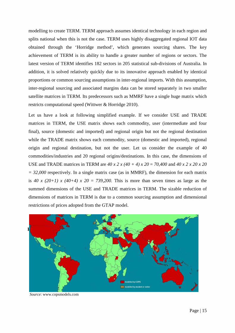
Source: www.copsmodels.com

Figure 2.1 CoPS style models in the world (not including GTAP)

Page | 16

TERM has been used in various analyses, including natural disasters (Horridge, Madden &

Wittwer 2005), agricultural management (Wittwer 2012), mining booms (Horridge &

Wittwer 2006) and infrastructure development (Horridge & Wittwer 2008). The model

provides opportunities to analyse the effects of small-region specific policy changes such as

tourism impacts. TERM has also been served as a platform for the development of multi-

regional models for several countries including China (Horridge & Wittwer 2008) and

Indonesia (Horridge & Wittwer 2006). Figure 2.1 shows the countries for which CoPS style

models (not including GTAP) have been developed and used in policy analysis.

3. A General form of CoPS style CGE model

Let us define a general CoPS style model by:

𝐹𝐹(𝑋𝑋) = 0 (3)

where F is an m-vector of differentiable functions of n variables X.

For CGE models, n>m is generally the case. Each equation explains a variable but since

n>m, values for some variables must be set by the modeller (or model user). The variables

determined by the equations of the model are called endogenous variables and the variables

determined by the model user are called exogenous variables. The ‘closure’ of a model is a

selection of variables into endogenous and exogenous categories. One of the advantages of

CoPS style modelling is the freedom to employ a variety of different closures. Dixon (2006)

highlighted the importance of flexible closure and wrote that ‘an early insight at the IMPACT

project was that the division of variables into the endogenous and exogenous categories

should be flexible so that it can be varied from application to application’ in retrospect (p. 9).

Simple closure changes enable a CGE model to run with different underlying theories.

Hence, we can imply that the closures reflect the economic theories under consideration.

Closures allow us to do simulations in different environments: in the short or long run; with

flexible or sticky wages; with neoclassical or new Keynesian pricing; with fixed or variable

tax rates; and with a balanced or cyclical budget (Dixon & Rimmer 2002). Thus the closures

must reflect the details of the economic question under investigation. In dynamic successors

of ORANI, there are four basic closures: the historical closure, the decomposition closure, the

forecast closure and the policy closure.

Page | 17

In addition to the closure, another important tool to solve a CGE model is a numeraire.

Broadly speaking, a numaraire is the essential standard of measurement that enables the

comparison of values relative to a common unit or denominator. Traditional CoPS style CGE

models follow a neoclassical property in which economic agents respond to changes in

relative prices. There should be at least one exogenous variable measured in domestic

currency. The relative prices of all commodities and inputs are specified and measured by a

numeraire. Hence, all prices change relative to the numeraire. The choice of a numeraire is

up to modellers and model users depending on the economic environment. During the years

of fixed exchange regime, a nominal exchange rate was commonly used as a numeraire. With

new and neo Keynesian wage rigidity, a nominal wage has often been used as a numeraire.

4. Solution methods

Many of the equations in CoPS style models are essentially non-linear. Following Johansen,

the models are solved by representing them as a series of linear equations relating percentage

changes in model variables. There are two main approaches for solving CGE models: non-

linear programming and derivative methods. Today, almost all CGE models are solved by the

derivative method (Adams et al. 1994). The main advantage of the derivative method is that it

provides the matrix of an initial solution and generates deviations in endogenous variables

from their initial values created by deviations in exogenous variables from their initial values.

The derivative method works by replacing the non-linear levels representation of the model

with a linear first-order differential representation. The replacement can be either explicit or

implicit. The explicit approach involves equations presented to the computer in linear first

order differential form and the implicit approach involves equations presented in nonlinear

form and converted to differential form in the computer via numerical means.

The derivative method used in CoPS style models is the Johansen/Euler method developed by

Dixon et al. (1982) and implemented through GEMPACK with explicit representation of the

linear first-order differential form named in recognition of the Johansen and Euler. By

contrast, the World Bank tradition models are solved in implicit representation implemented

through the GAMS. As emphasised in Dixon and Rimmer (2002), there are two advantages

of explicit representation over the implicit representation: transparency of underlying

economics of a model and the detectability of computational problems. In addition, the

percentage change of a variable is a relative change whereas a change in the variable itself

represents an absolute change. Thus, the percentage change is generally more interesting and

more useful for comparative purposes.

Page | 18

This section explains solution methods and their applications to CoPS style models.

4.1. Johansen solution procedure

As in equation (3), a CoPS style model can be defined as an equilibrium vector, X, of length n

variables satisfying a system of equations. F is a vector of functions of length m, where n >

m. The Johansen approach is to derive from (3) a system of linear equations in which the

variables are changes, percentage changes or changes in the logarithms of the components of

X. Since the system (3) contains more variables than equations, we need to assign

exogenously given values to n-m variables and solve for the remaining m endogenous

variables.

The Johansen solution procedure can be defined using the following steps.

First, the system of equations for the model is represented in its original levels form as

𝐹𝐹(𝑋𝑋) = 0;

where F is an m-vector of differentiable functions of n level variables X.

Second, the total differential is taken of each equation in the model;

Third, the expressions for the total differential of each equation are expressed in

percentage change form.

In our case, we obtain:

𝐴𝐴(𝑋𝑋)𝑥𝑥 = 0

where 𝐴𝐴(𝑋𝑋) is and 𝑛𝑛 × 𝑚𝑚 matrix whose components are functions of X. 𝑥𝑥 is the

vector of percentage changes in X.

Fourth, the percentage change equations are evaluated at an initial solution to the

levels form.

𝐴𝐴(𝑋𝑋) is evaluated at 𝑋𝑋 = 𝑋𝑋𝐼𝐼.

Fifth, a closure of the model is defined. Then, the model is solved for the percentage

change movements in the endogenous variables away from their initial values given

changes in the exogenous variables.

𝐴𝐴𝛼𝛼(𝑋𝑋𝐼𝐼)𝑥𝑥𝛼𝛼 + 𝐴𝐴𝛽𝛽(𝑋𝑋𝐼𝐼)𝑥𝑥𝛽𝛽 = 0;

where 𝑥𝑥𝛼𝛼 is the 𝑚𝑚×1 sub-vector of endogenous components of 𝑥𝑥;

Then the model is solved, assuming that the relevant inverse matrix exists:

𝑥𝑥𝛼𝛼 = −𝐴𝐴𝛼𝛼−1(𝑋𝑋𝐼𝐼)𝐴𝐴𝛽𝛽(𝑋𝑋𝐼𝐼)𝑥𝑥𝛽𝛽

More compactly we can write it as:

Page | 19

𝑥𝑥𝛼𝛼 = 𝐵𝐵(𝑋𝑋𝐼𝐼)𝑥𝑥𝛽𝛽;

where 𝐵𝐵(𝑋𝑋𝐼𝐼) = −𝐴𝐴𝛼𝛼−1(𝑋𝑋𝐼𝐼)𝐴𝐴𝛽𝛽(𝑋𝑋𝐼𝐼).

𝐴𝐴(𝑋𝑋𝐼𝐼) matrix defined in Johansen solution procedure is called the Tableau matrix. The

Tableau matrix shows the sensitivity (elasticity in our example since we defined 𝑥𝑥 as a

percentage change) of every endogenous variable with respect to every exogenous variable.

In his seminal work, Johansen used the Tableau matrix to decompose movements in industry

outputs, prices and primary factor inputs into parts attributable to observed changes in six sets

of exogenous variables: aggregate employment; aggregate capital; population; Hicks-neutral

primary factor technical change in each industry; exogenous demand for each commodity;

and the price of non-competing imports. Hence, the Tableau matrix enables us to understand

the CGE model and its results, to assess it against reality or to do the checking of computed

results (Dixon & Rimmer 2010a).

Due to linearization, the deviation from true value or linearization error may occur. The

larger the shock, the greater the proportional linearization error is in general. Johansen

recognized the linearization error in his computations and acknowledged that the solutions

from his model were approximate.

4.2. Johansen/Euler solution procedure

Dixon et al. (1982) set out an extension to the Johansen method which eliminates

linearization errors while retaining the simplifying advantages of linearized algebra. They

employed Euler’s method and added multiple steps. The Johansen method described above

can be interpreted as a one-step Euler solution.

Johansen/Euler solution procedure breaks up the shock into a number of equal parts or steps.

The linearized model is solved in each step for smaller shocks. After each step, the value of

every endogenous variable affected by the shock is updated. In general, the more steps the

shock is broken into, the more accurate the results are. However, for the level of convergence

toward the true solution that the Euler method provides, it is computationally expensive.

4.3. Gragg’s method

Gragg’s method is very similar to Johansen/Euler method with some slight difference. When

the shocks are broken into N parts, Euler's method does N separate calculations while Gragg's

method does N + 1. It is more accurate than Euler's method for calculating the direction in

which to move at each step. The default method in GEMPACK used for solving the GTAP

model, for instance, is Gragg’s method with Richardson’s extrapolation.

Page | 20

4.4. Richardson’s extrapolation

Richardson’s extrapolation infers the results for an Euler or Gragg simulation of an infinite

number of steps by using information on the rate at which the gap between simulations of

different step sizes changes as the number of steps increases.

If we denote the results for endogenous variables from Euler/Gragg simulation of N steps as

R(N), the following approximation often holds for CoPS style model simulations:

(1) 𝑅𝑅(2) − 𝑅𝑅(1) ≈ 2(𝑅𝑅(4) − 𝑅𝑅(2))

……………………………

(∞) 𝑅𝑅(∞) ≈ 2.𝑅𝑅(2) − 𝑅𝑅(1))

When Euler method is supplemented with Richardson’s extrapolation, the number of steps

(N) can be very small. As we can see from (∞), the number of steps can be 2 in normal

applications of the model. Pearson (1991) showed multi-step Euler method complemented

with Richardson’s extrapolation can solve CoPS style CGE models with any desired degree

of precision.

5. Standard notations and conventions

This section introduces the notations and conventions used in CoPS style modelling. One of

the distinctive technical characteristics of CoPS style models is the naming system invented

with ORANI for ease of reference. There are four types of notations in CoPS style models.

The first type is a ‘letter’ notation. Lowercase symbols are used to represent percentage

changes in the variables denoted by the corresponding uppercase symbols. For instance, a, p,

w and x represent the percentage changes in A, P, V and X where they are technology

parameter, price, value, and quantity respectively. The second one is a ‘number’ notation.

One of the digits 0 to 6 indicates and identifies the user. The third type is ‘a combination of

letters’ for further information. For example, TOT denotes total over all inputs for some user,

MAR represents margins and LAB indicates labour.

To illustrate the second and third types of standard notation, let us have a look at the identity

below where total supply of output in an economy is equal to the total use:

Page | 21

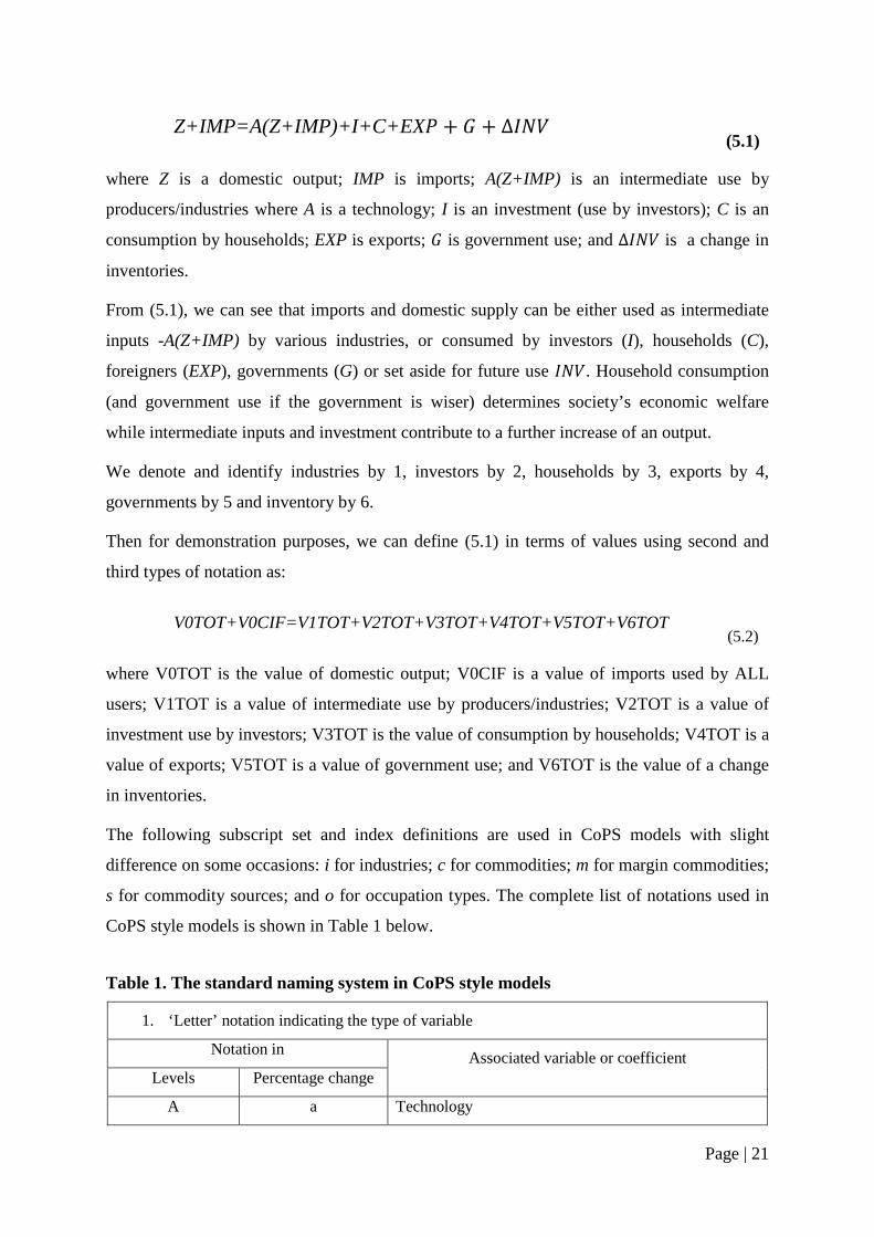
Z+IMP=A(Z+IMP)+I+C+EX𝑃𝑃 + 𝐺𝐺 + ∆𝐼𝐼𝐼𝐼𝐼𝐼 (5.1)

where Z is a domestic output; IMP is imports; A(Z+IMP) is an intermediate use by

producers/industries where A is a technology; I is an investment (use by investors); C is an

consumption by households; EXP is exports; 𝐺𝐺 is government use; and ∆𝐼𝐼𝐼𝐼𝐼𝐼 is a change in

inventories.

From (5.1), we can see that imports and domestic supply can be either used as intermediate

inputs -A(Z+IMP) by various industries, or consumed by investors (I), households (C),

foreigners (EXP), governments (G) or set aside for future use 𝐼𝐼𝐼𝐼𝐼𝐼. Household consumption

(and government use if the government is wiser) determines society’s economic welfare

while intermediate inputs and investment contribute to a further increase of an output.

We denote and identify industries by 1, investors by 2, households by 3, exports by 4,

governments by 5 and inventory by 6.

Then for demonstration purposes, we can define (5.1) in terms of values using second and

third types of notation as:

V0TOT+V0CIF=V1TOT+V2TOT+V3TOT+V4TOT+V5TOT+V6TOT (5.2)

where V0TOT is the value of domestic output; V0CIF is a value of imports used by ALL

users; V1TOT is a value of intermediate use by producers/industries; V2TOT is a value of

investment use by investors; V3TOT is the value of consumption by households; V4TOT is a

value of exports; V5TOT is a value of government use; and V6TOT is the value of a change

in inventories.

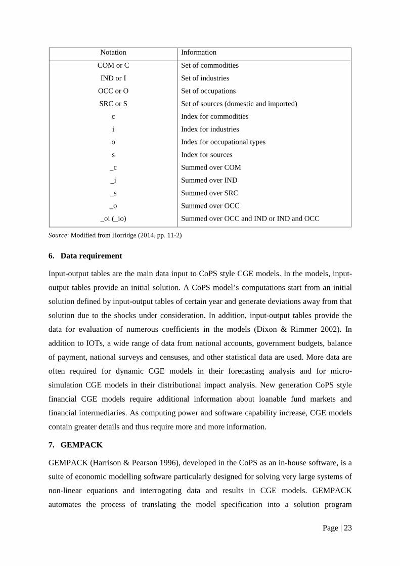
The following subscript set and index definitions are used in CoPS models with slight

difference on some occasions: i for industries; c for commodities; m for margin commodities;

s for commodity sources; and o for occupation types. The complete list of notations used in

CoPS style models is shown in Table 1 below.

Table 1. The standard naming system in CoPS style models

1. ‘Letter’ notation indicating the type of variable

Notation in Associated variable or coefficient Levels Percentage change

A a Technology

Page | 22

P

PF

X

V

T

F

p

pf

x

w

t

f

Price, local currency

Price, foreign currency

Input quantity

Value, local currency

Tax

Shifter

2. ‘Number’ notation indicating user

Notation User

1

2

3

4

5

6

0

Current production (industries)

Investment (investors)

Consumption (households)

Export (foreigners)

Government(s)

Inventories

All users, or user distinction irrelevant

3. ‘Combination of letters’ notation for further information

Notation Information

BAS or bas

CAP or cap

CIF or cif

DOM or dom

FAC or fac

IMP or imp

LAB or lab

LND or lnd

LUX or lux

MAR or mar

OCT or oct

PRIM or prim

PUR or pur

SUB or sub

TAR or tar

TAX or taxes

TOT or tot

Basic

Capital

Imports at border prices

Domestic

All factors

Imports (duty paid) or imported

Labour

Land

Linear expenditure system (supernumerary part)

Margin

Other cost tickets

All primary factors

At purchaser’s prices

Linear expenditure system (subsistence part)

Tariffs

Taxes

Total or average over all inputs for some user

4. Sets, indices and other notations

Page | 23

Notation Information

COM or C

IND or I

OCC or O

SRC or S

c

i

o

s

_c

_i

_s

_o

_oi (_io)

Set of commodities

Set of industries

Set of occupations

Set of sources (domestic and imported)

Index for commodities

Index for industries

Index for occupational types

Index for sources

Summed over COM

Summed over IND

Summed over SRC

Summed over OCC

Summed over OCC and IND or IND and OCC

Source: Modified from Horridge (2014, pp. 11-2)

6. Data requirement

Input-output tables are the main data input to CoPS style CGE models. In the models, input-

output tables provide an initial solution. A CoPS model’s computations start from an initial

solution defined by input-output tables of certain year and generate deviations away from that

solution due to the shocks under consideration. In addition, input-output tables provide the

data for evaluation of numerous coefficients in the models (Dixon & Rimmer 2002). In

addition to IOTs, a wide range of data from national accounts, government budgets, balance

of payment, national surveys and censuses, and other statistical data are used. More data are

often required for dynamic CGE models in their forecasting analysis and for micro-

simulation CGE models in their distributional impact analysis. New generation CoPS style

financial CGE models require additional information about loanable fund markets and

financial intermediaries. As computing power and software capability increase, CGE models

contain greater details and thus require more and more information.

7. GEMPACK

GEMPACK (Harrison & Pearson 1996), developed in the CoPS as an in-house software, is a

suite of economic modelling software particularly designed for solving very large systems of

non-linear equations and interrogating data and results in CGE models. GEMPACK

automates the process of translating the model specification into a solution program

Page | 24

(Horridge 2014). The implementation of CGE models can be written in levels and equations,

percentage change equations or a mixture of them via algebra-like language used to describe

and document the implementation. Then the GEMPACK program TABLO translates these

texts into model-specific programs which solve the models. GEMPACK is equipped to

handle a wide range of economic behaviour and contains an advanced method solving inter-

temporal models with adaptive and rational expectations. It is used in over 500 organisations

in 100 countries.

A key motivation in designing and adopting GEMPACK was to allow economists to

construct and run models without the hassle of complicated algorithms. The advances in

GEMPACK, including user friendly Windows programs, have substantially increased

modellers’ and users’ productivity. Some of GEMPACK’s integrated development

environments can identify and zip up all the original or source files needed to produce a

simulation (Horridge et al. 2012). These developments have facilitated and expedited the

transfer of CGE technology across the world. GEMPACK’s speed to solve large CGE models

is substantially faster than its counterparts. GEMPACK can solve the equations using one of

four related solution methods: Johansen, Euler, Gragg’s or the midpoint methods discussed in

section 4. .

8. Back-of-The-Envelope (BOTE) Analysis

A back-of-the-envelope (BOTE) model is a small model which can be managed with pencil

and paper, designed to explain a particular application of a full-scale model. BOTE modelling

is as old as CGE modelling. In his seminal work, Johansen (1960) used a one-sector BOTE

model to guide his discussion of the huge number of results generated by his CGE model of

Norway’s economy. There has been a robust, well-established tradition among CoPS style

CGE modellers to use BOTE models and calculations for assessing model results. The usage

of BOTE models and calculations is one of the distinctive characteristics of CoPS style

modelling.

In the original ORANI publication (Dixon et al. 1977, pp. 194-9), BOTE models were

described as having the following roles:

First, there is a purely practical point. With a model as large as ORANI, the onus is on the model builders to provide convincing evidence that the computations have been performed correctly, i.e., that the results do in fact follow from the theoretical structure and database. Second [BOTE calculations are] the only way: to “understand” the model; to isolate those assumptions which ‘cause’

Page | 25

particular results; and to access the plausibility of particular results by seeing which real-world phenomena have been considered and which have been ignored. Third, … by modifying and extending [BOTE] calculations … the reader will be able to obtain reasonably accurate idea of how some of the projections would respond to various changes in the underlying assumptions and data.

Via well-designed BOTE calculations, the model builder can isolate the economic

mechanisms and data items that are important for a given set of results (Dixon & Rimmer

2002). In general, BOTE models and BOTE calculations are for explaining particular results

from the full scale model and validating the plausibility of model results. Dixon and Rimmer

(2002, pp. 108-9) identify the following five reasons for their emphasis on BOTE models and

calculations. First, BOTE models and calculations serve as a necessary check for data

handling and other coding errors. Second, they are capable of revealing result-affecting

theoretical limitations. Third, BOTE models and calculations allow modellers and users to

identify the principal mechanism and data items underlying particular results. Fourth, they are

an effective form of sensitivity analysis. Fifth, BOTE models and calculations generate new

theoretical insights and propositions. The nature of the BOTE models can be varied from

application to application. For an ORANI simulation of an increase in oil prices, the

corresponding BOTE model included the price of oil and the share of oil in the economy’s

production costs (Dixon et al., 1984). For an ORANI simulation of the effects of a tariff

increase, the corresponding BOTE model included a tariff rate (Dixon et al., 1977, pp. 214-

222). A large number of different types of BOTE equations and equation systems in levels

and percentage change have been developed and used in CoPS style models.

Page | 26

References

Adams, PD 1989, 'Incorporating financial assets into ORANI: the extended Walrasian paradigm', University of Melbourne.

Adams, PD, Dixon, PB, McDonald, D, Meagher, GA & Parmenter, BR 1994, 'Forecasts for

the Australian economy using the MONASH model', International Journal of Forecasting, vol. 10, no. 4, pp. 557-71.

Adams, PD, Horridge, M & Parmenter, BR 2000a, MMRF-GREEN: A Dynamic, Multi-

Sectoral, Multi-Regional Model of Australia, Victoria University, Centre of Policy Studies/IMPACT Centre.

Adams, PD, Horridge, M, Parmenter, BR & Zhang, XG 2000b, 'Long‐run Effects on China of

APEC Trade Liberalization', Pacific Economic Review, vol. 5, no. 1, pp. 15-47. Anderson, K 2014, Australia's Economy in its International Context, vol. II, 2 vols.,

University of Adelaide Press, Adelaide, SA. Anderson, K, Giesecke, J & Valenzuela, E 2010, 'How would global trade liberalization

affect rural and regional incomes in Australia?', Australian Journal of Agricultural and Resource Economics, vol. 54, no. 4, pp. 389-406.

Anderson, K, Martin, W & Van der Mensbrugghe, D 2012, 'Estimating effects of price-

distorting policies using alternative distortions databases', in Handbook of Computable General Equilibrium Modeling, Oxford, pp. 877-932.

Armington, PS 1969, 'The Geographic Pattern of Trade and the Effects of Price Changes

(Structure géographique des échanges et incidences des variations de prix) (Estructura geográfica del comercio y efectos de la variación de los precios)', Staff Papers (International Monetary Fund), vol. 16, no. 2, pp. 179-201.

Bandara, J 1991a, 'An investigation of “Dutch disease” economics with a miniature CGE

model', Journal of Policy Modeling, vol. 13, no. 1, pp. 67-92. Bandara, J 1991b, 'Computable general equilibrium models for development policy analysis

in LDCs', Journal of economic surveys, vol. 5, no. 1, pp. 3-69. Brooke, A, Kendrick, D & Meeraus, A 1996, GAMS Release 2.25: A user's guide, GAMS

Development Corporation Washington, DC. Burniaux, J-M & Truong, TP 2002, 'GTAP-E: an energy-environmental version of the GTAP

model', GTAP Technical Papers, p. 18. Corden, WM 1995, Protection and liberalization in Australia and abroad, University of

Adelaide. Coxhead, IA & Warr, PG 1995, 'DOES TECHNICAL PROGRESS IN AGRICULTURE

ALLEVIATE POVERTY? A PHILIPPINE CASE STUDY*', Australian Journal of Agricultural Economics, vol. 39, no. 1, pp. 25-54.

Page | 27

Coxhead, IA, Warr, PG & Crawford, J 1991, 'Technical change, land quality, and income

distribution: a general equilibrium analysis', American Journal of Agricultural Economics, vol. 73, no. 2, pp. 345-60.

Dee, PS 1994, General equilibrium models and policy advice in Australia, Australian

Government Pub. Service. Dervis, K & Robinson, S 1982, General equilibrium models for development policy,

Cambridge university press. Dixon, PB 1975, The theory of joint maximization, vol. 91, North-Holland Publishing

Company. Dixon, PB 1978, 'The computation of economic equilibria: A joint maximization approach',

Metroeconomica, vol. 30, no. 1‐2‐3, pp. 173-85. Dixon, PB 2006, 'Evidence-based Trade Policy Decision Making in Australia and the

Development of Computable General Equilibrium Modelling'. Dixon, PB & Butlin, MW 1977, 'Notes on the Evans Model of Protection*', Economic

Record, vol. 53, no. 3, pp. 337-49. Dixon, PB, Giesecke, JA & Rimmer, MT 2015, 'Superannuation within a financial CGE

model of the Australian economy ', paper presented to GTAP 18th Annual Conference on Global Economic Analysis, Melbourne.

Dixon, PB & Jorgenson, D 2013, Handbook of Computable General Equilibrium Modeling

SET, Vols. 1A and 1B, Newnes. Dixon, PB, Koopman, R & Rimmer, MT 2013, 'The MONASH style of CGE modeling: a

framework for practical policy analysis', Chapter, vol. 2, pp. 23-102. Dixon, PB & Parmenter, BR 1996, 'Computable general equilibrium modelling for policy

analysis and forecasting', Handbook of computational economics, vol. 1, pp. 3-85. Dixon, PB, Parmenter, BR, Powell, AA & Wilcoxen, PJ 1992, 'Notes and problems in

applied general equilibrium analysis', Advanced Textbooks in Economics, no. 32. Dixon, PB, Parmenter, BR, Ryland, GJ & Sutton, JP 1977, ORANI, a general equilibrium

model of the Australian economy: Current specification and illustrations of use for policy analysis.

Dixon, PB, Parmenter, BR, Sutton, J & Vincent, DP 1982, ORANI: A Multisectoral Model of

the Australian Economy, North-Holland Publishing Company, Amsterdam. Dixon, PB, Powell, AA & Harrower, JD 1977, Long Term Structural Pressures on Industries

and the Labour Market, IMPACT Project.

Page | 28

Dixon, PB & Rimmer, MT 2002, Dynamic General Equilibrium Modelling for Forecasting and Policy: A Practical Guide and Documentation of MONASH, Contribution to Economic Analysis, North Holland, Amsterdam.

Dixon, PB & Rimmer, MT 2005, 'Mini-USAGE: Reducing Barriers to Entry in Dynamic

CGE Modelling.”', in 8th Annual Conference on Global Economic Analysis, Lübeck, Germany, and June.

Dixon, PB & Rimmer, MT 2010, Johansen’s Contribution to CGE Modelling: Originator

and Guiding Light for 50 Years, G-203, Centre of Policy Studies, Monash University, Melbourne.

Dixon, PB & Rimmer, MT 2010a, Johansen's contribution to CGE modelling: originator and

guiding light for 50 years, Monash University, Centre of Policy Studies and the Impact Project.

Edgeworth, FY 1881, Mathematical psychics: An essay on the application of mathematics to

the moral sciences, CK Paul. Elliott, AC & Woodward, WA 2007, Statistical analysis quick reference guidebook: With

SPSS examples, Sage. Evans, HD 1972, A General Equilibrium Analysis of Protection: the Effects of Protection in

Australia, North-Hollan Publishing Company, Amsterdam. Giesecke, JA 2000, 'FEDERAL-F: A multi-regional multi-sectoral dynamic model of the

Australian economy'. Giesecke, JA 2011, 'Development of a large-scale single US region CGE model using

IMPLAN data: A Los Angeles County example with a productivity shock application', Spatial Economic Analysis, vol. 6, no. 3, pp. 331-50.

Giesecke, JA & Madden, JR 2013, 'Regional computable general equilibrium modeling',

Handbook of Computable General Equilibrium Modeling, vol. 1, pp. 379-475. Gregory, RG 1976, 'SOME IMPLICATIONS OF THE GROWTH OF THE MINERAL

SECTOR*', Australian Journal of Agricultural Economics, vol. 20, no. 2, pp. 71-91. Harrison, WJ & Pearson, KR 1996, 'Computing solutions for large general equilibrium

models using GEMPACK', Computational Economics, vol. 9, no. 2, pp. 83-127. Hertel, T 1997, Global trade analysis: modeling and applications, Cambridge university

press, USA. Hertel, T 2013, 'Global applied general equilibrium analysis using the global trade analysis

project framework', in Handbook of Computable General Equilibrium Modeling, Oxford, UK, vol. 1B, pp. 815-76.

Page | 29

Horridge, M 2000, ORANI-G: A General Equilibrium Model of the Australian Economy, OP-93, Centre of Policy Studies, Victoria University, <http://www.copsmodels.com/elecpapr/op-93.htm>.

Horridge, M 2014, 'ORANI-G: A generic single-country computable general equilibrium

model', Centre of Policy Studies—CoPS. Monash University. Austrália. Horridge, M, Madden, J & Wittwer, G 2005, 'The impact of the 2002–2003 drought on

Australia', Journal of Policy Modeling, vol. 27, no. 3, pp. 285-308. Horridge, M, Parmenter, BR, Cameron, M, Joubert, R, Suleman, A & de Jongh, D 1995, The

macroeconomic, industrial, distributional and regional effects of government spending programs in South Africa, Victoria University, Centre of Policy Studies/IMPACT Centre.

Horridge, M, Parmenter, BR & Pearson, KR 1993, 'ORANI-F: A General Equilibrium

Model', Economic and Financial Computing, vol. 3, no. 2, pp. 71-140. 1998, ORANI-G: A General Equilibrium Model of the Australian Economy, by Horridge, M,

Parmenter, BR & Pearson, KR, Monash University, Centre of Policy Studies and the Impact Project.

Horridge, M, Pearson, K, Meeraus, A & Rutherford, T 2012, Solution Software for CGE

Modeling. chapter 20 in: Dixon PB, Jorgensen D.(eds), Handbook of CGE modeling, Elsevier. ISBN.

Horridge, M & Wittwer, G 2006, The Impacts of Higher Energy Prices on Indonesia’s and

West Java’s Economies using INDOTERM, a Multiregional Model of Indonesia, Department of Economics, Padjadjaran University.

Horridge, M & Wittwer, G 2008, 'SinoTERM, a multi-regional CGE model of China', China

Economic Review, vol. 19, no. 4, pp. 628-34. Johansen, L 1960, A multi-sector study of economic growth, vol. 21, North-Holland Pub. Co. Jomini, P, McDougall, R, Watts, G & Dee, PS 1994, The SALTER Model of the World

Economy: Model, Structure, Database and Parameters, Industry Commission, Melbourne.

Leontief, WW 1936, 'Quantitative input and output relations in the economic systems of the

United States', The review of economic statistics, pp. 105-25. Leontief, WW 1951, 'Input-output economics', Sci Am, vol. 185, no. 4, pp. 15-21. Leontief, WW, Morgan, A, Polenske, K, Simpson, D & Tower, E 1965, 'The economic

impact--industrial and regional--of an arms cut', The Review of Economics and Statistics, pp. 217-41.

Mackinnon, JG 1976, 'The Theory of Joint Maximization (Book)', Canadian Journal of

Economics, vol. 9, no. 4, p. 733.

Page | 30

Madden, JR 1990, 'FEDERAL: A two-region multisectoral fiscal model of the Australian

economy', University of Tasmania. Mai, Y, Dixon, PB & Rimmer, MT 2010, CHINAGEM: A Monash-styled dynamic CGE

model of China, Centre of Policy Studies and the Impact Project. Manne, AS 1963, 'Key Sectors of the Mexican Economy, 1960-1970', Studies in Process

Analysis Cowles Foundation Monograph, vol. 18. Marshall, A 1890, 'Principles of political economy', Maxmillan, New York. Nana, G & Philpott, B 1983, The 38 Sector Joanna Model, Victoria University of Wellington,

Research Project on Economic Planning. Naqvi, F & Peter, MW 1996, 'A MULTIREGIONAL, MULTISECTORAL MODEL OF

THE AUSTRALIAN ECONOMY WITH AN ILLUSTRATIVE APPLICATION*', Australian Economic Papers, vol. 35, no. 66, pp. 94-113.

Parmenter, B 2004, Distinguished Fellow of the Economic Society of Australia, 2003: Peter

Dixon, Wiley-Blackwell, 00130249, Other. PC 2003a, 'From industry assistance to productivity: 30 years of ‘the Commission’',

Melbourne: Productivity Commission. Pearson, KR 1991, Solving nonlinear economic models accurately via a linear

representation, Victoria University, Centre of Policy Studies/IMPACT Centre. Peter, MW, Horridge, M, Meagher, GA, Naqvi, F & Parmenter, BR 1996, The theoretical

structure of MONASH-MRF, Victoria University, Centre of Policy Studies/IMPACT Centre.

Powell, AA 2007, '“Why, How and When did GTAP Happen? What has it Achieved? Where

is ti Heading?”', GTAP Working Paper, vol. 38. Powell, AA & Snape, R 1992, 'The Contribution of Applied General Equlibrium Analysis to

Policy Reform in Australia', CoPS/Impact Project Paper series, vol. General paper, no. No G-98.

Sandee, J 1960, A Demonstration Planning Model for India, Asia Publishin House, Calcutta. Scarf, H 1967, 'The Approximation of Fixed Points of a Continuous Mapping', SIAM Journal

on Applied Mathematics, vol. 15, no. 5, pp. 1328-43. Scarf, H & Hansen, T 1973, 'The computation of economic equilibria', New Haven. Shoven, JB & Whalley, J 1992, Applying general equilibrium, Cambridge university press. Vincent, DP 1982, 'Effects of Higher Oil Prices on Resource Allocation and Living

Standards: The Case of Korea', The Developing Economies, vol. 20, no. 3, pp. 279-300.

Page | 31

Vincent, DP 1991, An Economy-wide model of Papua New Guinea: theory, data and

implementation, National Centre for Development Studies. Walras, L 1877, Elements of pure economics, Routledge. Wittwer, G 1999, WAYANG: a general equilibrium model adapted for the Indonesian

economy, Centre for International Economic Studies. Wittwer, G 2012, Economic Modeling of Water: The Australian CGE Experience, vol. 3,

Springer Science & Business Media. Wittwer, G & Anderson, K 1999, 'Accounting for Growth in Australia's Grape and Wine

Industries 1986 to 2003', vol. 99, no. 2. Wittwer, G & Horridge, M 2010, 'Bringing regional detail to a CGE model using census

data', Spatial Economic Analysis, vol. 5, no. 2, pp. 229-55.