coordinating tax reforms in the poorest...

Policy Research Working Paper 5919

Coordinating Tax Reforms in the Poorest Countries

Can Lost Tariffs be Recouped?

Swarnim Waglé

The World BankPoverty Reduction and Economic Management NetworkInternational Trade DepartmentDecember 2011

WPS5919P

ublic

Dis

clos

ure

Aut

horiz

edP

ublic

Dis

clos

ure

Aut

horiz

edP

ublic

Dis

clos

ure

Aut

horiz

edP

ublic

Dis

clos

ure

Aut

horiz

edP

ublic

Dis

clos

ure

Aut

horiz

edP

ublic

Dis

clos

ure

Aut

horiz

edP

ublic

Dis

clos

ure

Aut

horiz

edP

ublic

Dis

clos

ure

Aut

horiz

ed

Produced by the Research Support Team

Abstract

The Policy Research Working Paper Series disseminates the findings of work in progress to encourage the exchange of ideas about development issues. An objective of the series is to get the findings out quickly, even if the presentations are less than fully polished. The papers carry the names of the authors and should be cited accordingly. The findings, interpretations, and conclusions expressed in this paper are entirely those of the authors. They do not necessarily represent the views of the International Bank for Reconstruction and Development/World Bank and its affiliated organizations, or those of the Executive Directors of the World Bank or the governments they represent.

Policy Research Working Paper 5919

A revenue-neutral switch from trade taxes to domestic consumption taxes is fraught with implementation challenges in countries with a large informal sector. It is shown for a sample of low-income countries over 25 years that they have had a mixed record of offsetting reductions in trade tax revenue. The paper then analyzes the specific case of Nepal, using a unique data set compiled from unpublished customs records of imports, tariffs and all other taxes levied at the border. It estimates changes to revenue and domestic production associated with two sets

This paper is a product of the International Trade Department, Poverty Reduction and Economic Management Network. It is part of a larger effort by the World Bank to provide open access to its research and make a contribution to development policy discussions around the world. Policy Research Working Papers are also posted on the Web at http://econ.worldbank.org. The author may be contacted at [email protected].

of reforms: i) proportional tariff cuts coordinated with a strictly enforced value-added tax; and ii) proposed tariff cuts under a regional free trade agreement. It is shown that a revenue-neutral tax reform is conditional on the effectiveness with which domestic taxes are enforced. Furthermore, loss of revenue as a result of intra-regional free trade can be minimized through judicious use of Sensitive Lists that still cover substantially all the trade as required by Article XXIV of the GATT.

C O O R D I N AT I N G TA X R E F O R M S I N T H E P O O R E S T C O U N T R I E S :C A N L O S T TA R I F F S B E R E C O U P E D ?

swarnim waglé1

Abstract

A revenue-neutral switch from trade taxes to domestic consumption taxes is fraught with im-plementation challenges in countries with a large informal sector. It is shown for a sample oflow-income countries over 25 years that they have had a mixed record of offsetting reductionsin trade tax revenue. The paper then analyzes the specific case of Nepal, using a unique dataset compiled from unpublished customs records of imports, tariffs and all other taxes levied atthe border. It estimates changes to revenue and domestic production associated with two sets ofreforms: i) proportional tariff cuts coordinated with a strictly enforced value-added tax; and ii)proposed tariff cuts under a regional free trade agreement. It is shown that a revenue-neutral taxreform is conditional on the effectiveness with which domestic taxes are enforced. Furthermore,loss of revenue as a result of intra-regional free trade can be minimized through judicious use ofSensitive Lists that still cover substantially all the trade as required by Article XXIV of the GATT.

Keywords: tariff, tax revenue, trade adjustment, NepalJEL Classification: F13, F21, H20, O17

Sector Board: EPOL

1 Consultant, The World Bank. I am grateful to Prema-chandra Athukorala for helpful commentsand guidance. I thank Paul Brenton, Mombert Hoppe and Olivier Jammes for facilitating the useof the Tariff Reform Impact Simulation Tool (TRIST) developed by the World Bank. I also thankNepali officials in the Ministry of Finance and the Department of Customs for granting me accessto the Automated System for Customs Data (ASYCUDA). And I acknowledge with gratitude ThomasBaunsgaard and Michael Keen of the International Monetary Fund (IMF) for sharing their data seton taxes. All errors are mine.

C O N T E N T S

Table of Contents iiList of Figures ivList of Tables ivAcronyms v1 coordinating tax reforms : can lost tariffs be recouped? 1

1.1 Introduction . . . . . . . . . . . . . . . . . . . . . . . . . . . . . . . . . 1

1.2 Cross-Country Evidence on Revenue Recovery . . . . . . . . . . . . . 5

1.2.1 Econometric Model . . . . . . . . . . . . . . . . . . . . . . . . 5

1.2.2 Data . . . . . . . . . . . . . . . . . . . . . . . . . . . . . . . . . 7

1.2.3 Estimation Method . . . . . . . . . . . . . . . . . . . . . . . . . 8

1.2.4 Results . . . . . . . . . . . . . . . . . . . . . . . . . . . . . . . . 9

1.3 Joint Trade-Fiscal Reform: A Case Study . . . . . . . . . . . . . . . . 13

1.3.1 Theoretical Motivation . . . . . . . . . . . . . . . . . . . . . . . 14

1.3.2 Simulation Model . . . . . . . . . . . . . . . . . . . . . . . . . . 19

1.3.3 Data . . . . . . . . . . . . . . . . . . . . . . . . . . . . . . . . . 21

1.3.4 Results . . . . . . . . . . . . . . . . . . . . . . . . . . . . . . . . 25

1.3.5 Robustness . . . . . . . . . . . . . . . . . . . . . . . . . . . . . . 34

1.4 Related Issues in Tariff Reform . . . . . . . . . . . . . . . . . . . . . . 36

1.4.1 Change in Domestic Prices and Production . . . . . . . . . . . 36

1.4.2 Collected and Statutory Rates . . . . . . . . . . . . . . . . . . . 37

1.5 Conclusion . . . . . . . . . . . . . . . . . . . . . . . . . . . . . . . . . . 39

Appendix . . . . . . . . . . . . . . . . . . . . . . . . . . . . . . . . . . . . . . 47

1.A How the Model in TRIST Works . . . . . . . . . . . . . . . . . . . . . 47

1.B Additional Tables . . . . . . . . . . . . . . . . . . . . . . . . . . . . . . 51

iii

L I S T O F F I G U R E S

Figure 1 Contribution of Trade Taxes to Total Tax Revenue . . . . . . . 3

Figure 2 Share of Tax Revenue by Source . . . . . . . . . . . . . . . . . 24

Figure 3 Dispersion of Tariff Rates . . . . . . . . . . . . . . . . . . . . . 29

Figure 4 Statutory and Collected Tariff Rates . . . . . . . . . . . . . . . 38

L I S T O F TA B L E S

Table 1 Recovery of Taxes in Low-Income Countries, 1982-2006 . . . 11

Table 2 Illustration of Price and Demand Response in TRIST . . . . . 50

Table 3 Tariff Rates and Import-based Revenue in Nepal, 2008 . . . . 51

Table 4 VAT Collected on Imports, 2005-2010 . . . . . . . . . . . . . . 51

Table 5 Tariff Revenue by Band, 2008 . . . . . . . . . . . . . . . . . . . 51

Table 6 Impact on Revenue of Tariff and Tax Reforms . . . . . . . . . 52

Table 7 Impact on Revenue of Tariff and Tax Reforms with an Infor-mal Sector . . . . . . . . . . . . . . . . . . . . . . . . . . . . . . 53

Table 8 Impact on Revenue of Regional Free Trade . . . . . . . . . . . 54

Table 9 Impact on Revenue of Regional Free Trade with SensitiveLists . . . . . . . . . . . . . . . . . . . . . . . . . . . . . . . . . 55

Table 10 Robustness Tests with Higher Elasticities . . . . . . . . . . . . 56

Table 11 Change in Price, Production, Revenue, and Protection . . . . 57

Table 14 Statutory and Applied Tariff Rates . . . . . . . . . . . . . . . 58

Table 12 Major Exporters to Nepal, 2008 & 2010 . . . . . . . . . . . . . 58

Table 13 Number of Products in the Sensitive Lists . . . . . . . . . . . 58

Table 15 Summary of Data used in Table 1 Regressions . . . . . . . . . 59

Table 16 List of Countries and Related Tax Data, 2002-2006 . . . . . . 60

iv

A C R O N Y M S

ARF Agricultural Reform Fee

ASYCUDA Automated System for Customs Data

AVE Ad Valorem Equivalent

CGE Computable General Equilibrium

GATT General Agreement on Tariffs and Trade

GDP Gross Domestic Product

GMM Generalized Method of Moments

HS Harmonized Commodity Description and Coding System

IMF International Monetary Fund

ISIC International Standard Industrial Classification

IV Instrumental Variables

MFN Most Favored Nation

LDC Least Developed Countries

ROW Rest of the World

SAFTA South Asian Free Trade Area

SL Sensitive List

TRIST Tariff Reform Impact Simulation Tool

2SLS Two-Stage Least Squares

VAT Value-Added Tax

WGI World Governance Indicators

WTO World Trade Organization

v

1C O O R D I N AT I N G TA X R E F O R M S : C A N L O S T TA R I F F S B ER E C O U P E D ?

“Import tariffs should generally be ranked between four and twenty

percent ad valorem intended for [the monarch’s] revenue rather than

for trade limitation.”

– Kautilya, Arthashastra, circa 300 BC1

“Little else is requisite to carry a state to the highest degree of opulence

from the lowest barbarism, but peace, easy taxes, and a tolerable admin-

istration of justice.”

– Adam Smith, quoted in the Collected Works of Dugald Stewart, 17552

1.1 introduction

This paper analyzes the immediate revenue implications of trade and fiscal policy

reforms. The emphasis on “immediate” is important because over the long run, a

less distorted economy allocates resources better and is likely to contribute to eco-

nomic growth that widens the tax base. Liberalization thereby pays for itself over

time. Even in the short run it is not always the case that tariff cuts automatically

lead to revenue losses (Greenaway & Milner 1991).3 However, if the immediate

cost of potential revenue loss is not addressed, trade reforms are not only unlikely

to be undertaken, but they can be promptly reversed: Buffie (2001) cites at least

1 See Waldauer et al. (1996)

2 See section IV of Stewart (1755), emphasis added.3 This depends on the price elasticity of imports and exports, as well as the ability of the economy and

tax administrations to respond to altered incentives. Lowered tariffs reduce the incentive to smuggleand bring goods through the informal channels. Lower tariffs also stimulate increased imports. Thenature of trade liberalization also matters: while a gradually reforming country with a moderaterange of tariffs may lose revenue when it cuts them below a certain threshold, others that are still inthe process of converting quotas into tariffs could have a revenue windfall.

1

2 coordinating tax reforms : can lost tariffs be recouped?

12 episodes where revenue shortfalls triggered partial or full policy reversals in

recent decades.4

The conventional wisdom imparted in tax policy advice to developing coun-

tries over the past 30 years has been that domestic consumption or income taxes

are superior to trade taxes because the former can meet the government’s revenue

target with lower rates, a wider base, and without a protectionist bias. This is un-

derpinned by economic theory. Trade taxes introduce a wedge between foreign and

national prices which distort the allocation of resources by encouraging activities

in sectors that are viable only at prices above the world average. Dixit (1985) shows

that small, open economies are better off reducing tariffs to zero and depending

instead on destination-based consumption taxes.

As countries build capacities to extract tax revenue from income and domes-

tic consumption, the importance of trade taxes as a source of government finance

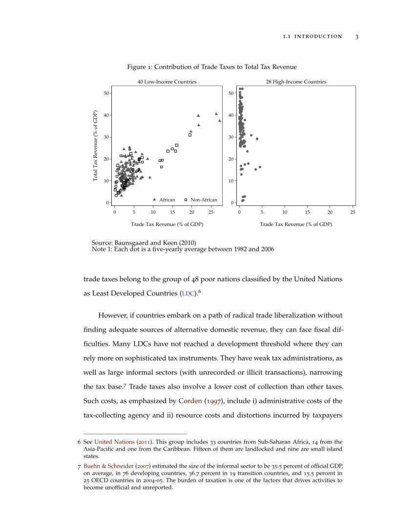
tends to decline.5 Figure 1 depicts this starkly with trade taxes being a substan-

tial portion of total tax revenues relative to Gross Domestic Product (GDP) in low-

income countries, but negligible in high-income countries. In the 1950s, developing

countries that are today classified as middle-income such as Colombia, Indonesia,

Malaysia, Nigeria, Sri Lanka and Thailand derived more than 40 percent of govern-

ment revenue from trade taxes (Lewis 1963; Corden 1997). By 1989, import duties

as a share of total tax revenue in developing countries were nearly 25 percent, on

average, but in developed countries only 2.7 percent (Burgess & Stern 1993). In

2009, customs and other import duties still accounted for more than 10 percent of

tax revenue in at least 24 countries. A majority of countries that rely excessively on

4 Philippines (1991), Kenya (1983), Morocco (1987), Guinea (1990, 1992), Bangladesh (late 1980s),Malawi (1980s), Senegal (after 1989), Costa Rica (1995), Mexico (1995), Brazil (1995), Colombia (1996).

5 Corden (1997) offers reasons why trade taxes become a less important source of government revenueas countries become rich: i) collection costs of non-trade tax like income fall; ii) the capacity of man-ufactured import-competing industries improve reducing the need for tariffs for either protection orrevenue; iii) as imports evolve from being associated with luxury to becoming part of the generalpopulation’s consumption basket, the progressive tax function played by tariffs diminishes; and iv)the pattern of imports shifts away from final consumer goods to intermediate and capital goods,because tariffs on intermediate goods lower effective protection for final goods, and are thereforelikely to be reduced.

1.1 introduction 3

Figure 1: Contribution of Trade Taxes to Total Tax Revenue

�

��

��

��

��

��

��

��

� � ��

��

��

��

�

��

��

��

��

��

� � ��

��

!�"�#$��

�� !"��#

trade taxes belong to the group of 48 poor nations classified by the United Nations

as Least Developed Countries (LDC).6

However, if countries embark on a path of radical trade liberalization without

finding adequate sources of alternative domestic revenue, they can face fiscal dif-

ficulties. Many LDCs have not reached a development threshold where they can

rely more on sophisticated tax instruments. They have weak tax administrations, as

well as large informal sectors (with unrecorded or illicit transactions), narrowing

the tax base.7 Trade taxes also involve a lower cost of collection than other taxes.

Such costs, as emphasized by Corden (1997), include i) administrative costs of the

tax-collecting agency and ii) resource costs and distortions incurred by taxpayers

6 See United Nations (2011). This group includes 33 countries from Sub-Saharan Africa, 14 from theAsia-Pacific and one from the Caribbean. Fifteen of them are landlocked and nine are small islandstates.

7 Buehn & Schneider (2007) estimated the size of the informal sector to be 35.5 percent of official GDP,on average, in 76 developing countries, 36.7 percent in 19 transition countries, and 15.5 percent in25 OECD countries in 2004-05. The burden of taxation is one of the factors that drives activities tobecome unofficial and unreported.


to minimize or evade payments, which if substantial could render trade taxes part

of a first-best tax package.

In this paper, I combine trade theory, cross-national evidence, and an in-depth

case study of a low-income country using a unique data set on all import transac-

tions at the border in Nepal.8 I find that low-income countries have had a mixed

record of achievement in offsetting reductions in trade tax revenue. This is partly

because of their weak enforcement of domestic taxes like Value-Added Tax (VAT).

In principle, a strict enforcement of a positive, single-rated VAT with no exemp-

tions is a highly effective form of modern taxation, and can negate substantial

losses in tariff revenue. I confirm this by using a partial equilibrium model to sim-

ulate reforms using data from Nepal on tariffs and up to ten additional domestic

taxes imposed on more than 400,000 import transactions between January 1 and

December 31, 2008.9

The paper proceeds as follows. Section 2 uses panel data from selected low-

income countries to assess whether they have succeeded in replacing trade taxes

with domestic sources over a period of 25 years. Given the limitations for country-

specific policy inference from cross-country regressions, sections 3 and 4 cover a

country case study. Section 3 begins by adapting conditions for welfare-enhancing

tariff cuts to a revenue-enhancing result from a coordinated tariff and tax reform in

the presence of an informal sector. Two sets of plausible policy reforms are then

simulated: i) different tariff cutting approaches are matched by domestic tax re-

forms with and without the assumption of a large informal sector; and ii) tariffs

and other discriminatory charges on imports from members party to the Agree-

ment on the South Asian Free Trade Area (SAFTA) are eliminated with and with-

out Sensitive Lists that exempt a subset of products from tariff cuts.10 I check for

8 “Border” in this paper refers to a generic port of entry. In many countries, a substantial share ofimports arrives by air into cities that may not technically be on the border.

9 In 2009-10, 22.5 percent of the government’s tax revenue was generated from tariffs on imports(Government of Nepal 2011).

10 Note that tariff cuts often take place as part of a broader package of trade policy reforms. Liber-alization of trade policy implies more than tariff cuts, for example, the conversion of quotas intotariffs, elimination of tariff exemptions and trade-related subsidies, reform of state-trading monop-

1.2 cross-country evidence on revenue recovery 5

robustness of results with different parameter assumptions of elasticities for prod-

uct substitution among exporters, between exporters and domestic producers, and

overall demand. Section 6 highlights two additional aspects of tariff reform. Sec-

tion 6 concludes.

1.2 cross-country evidence on revenue recovery

To set the stage for a detailed country case study subsequently, I examine in this

section the cross-national evidence from a sample of 40 low-income countries on

their record of replacing trade taxes with domestic sources over time. As trade

taxes as a share of GDP have altered, how have poor countries fared in terms

of domestic tax collection? In other words, for every dollar “lost” in trade taxes,

how many cents have they recouped through domestic sources? A cross-national

estimation of this nature requires a dynamic panel regression involving detailed

tax data that are not always publicly available. I, therefore, use internally compiled

IMF data and the estimation strategy of Baunsgaard & Keen (2010). I make three

major changes to their data and specification (explained later) to derive results for

revenue recovery by low-income countries that are comparable to, if not stronger

than the estimations in Baunsgaard and Keen (2005, 2010).

1.2.1 Econometric Model

The basic econometric specification is as in equation (1.1) where the dependent

variable is total domestic tax revenue (net of trade taxes) as a share of GDP (DTit).

Subscripts i and t indicate country and time, respectively.

DTit = αi +βoDTit−1 +β1TTit +β′2Xit + µt + εit (1.1)

olies, raising of low tariffs, elimination of export taxes, removal of foreign exchange rationing andimport licensing regimes, among others. Often these are coupled with macro-economic reforms toinfluence exchange rates, inflation, and incentives for investment.


The main explanatory variable of interest is trade tax revenue relative to GDP

(TTit). If its coefficient β1 is significantly negative, it can be concluded that a fall

in trade taxes has been associated with a rise in non-trade tax revenue. In the long

term, the relevant coefficient is −β1(1−βo)

. Time and country-fixed effects are captured

by µt and αi. The control variables (Xit) are those that affect either the costliness

of raising revenue from non-trade sources or the valuation of public expenditure.

If the marginal value of public expenditures foregone with lost trade taxes is high,

the urgency to seek alternative sources is greater. The control variabes are:

• GDP per capita: demand for government expenditures increases as average

incomes of citizens grow (Wagner’s Law). GDP per capita also proxies for

administrative and institutional capacity in the country to collect and man-

age taxes. (Institutional capacity is proxied better by measures of the quality

of governance like the World Governance Indicators (WGI), but their cross-

national time-series does not go as far back as the 1980s.)

• Imports: it is the share of total imports relative to GDP. It captures “openness”

of the economy as well as the fact that imports are a substantial part of

the domestic tax base in poor countries. Baunsgaard & Keen (2010) use for

openness a slightly broader measure: the share of exports and imports in

GDP, citing Rodrik (1998) who finds this measure of openness to be closely

associated with the size of government.

• Natural resources per capita: two measures are introduced as important con-

trols to capture the fact that states that derive a large share of revenues from

natural resources do not need to tax their citizens highly (Ross 2001).

• Foreign aid as a share of national income: this could have a perverse effect

on the urgency of finding an alternative source of domestic revenue.

• Share of agriculture in GDP: this measures the size of the economy that is

hard to tax, as well as the degree of informality prevailing in the economy.


• Inflation: reflects the extent to which revenue is generated from seigniorage,

which needs to be controlled for.

• VAT: a modern VAT regime that is strictly enforced is associated with in-

creased domestic revenue collection; however, a weakly enforced VAT system

with widespread exemptions could be revenue-reducing compared to taxes

collected at fixed border points.

1.2.2 Data

The IMF’s Government Finance Statistics is the best publicly accessible source

for cross-country data on tax revenue, but it is incomplete and suffers from mis-

measurement. I therefore use the same panel data as that used by Baunsgaard

& Keen (2010) who adjust the GFS data by cross-checking numbers with internal

IMF figures obtained through (“Article IV”) consultations with individual coun-

tries. They try to correct a common flaw in many countries where tariff and VAT

revenues are conflated if they are both collected at the border. This would be prob-

lematic for the exercise in this paper because the aim is to find out whether decline

in tariff revenues are made up for by domestic sources like VAT and excise.

I make three modifications to Baunsgaard and Keen’s data set. First, their data

on VAT is only a binary variable of whether the country had VAT in place in the

year concerned. I use in its place actual ad valorem rates, compiled from three

different sources as follows: Krever (2008), Ernst & Young (2008) and World Bank

2011a. Second, I confine my analysis to 40 low-income countries over a shorter

time period of 25 years, from 1982 to 2006.11 Third, I use two new measures for

a country’s abundance in natural resources as an additional explanatory variable.

The first measure is the per capita natural resource-based exports (belonging to

11 Five countries drop out of the regression because of incomplete data on inflation and per capitaincome, as follows: Comoros, Guinea, Myanmar, Sao Tome and Principe, and the Solomon Islands.


SITC Section 3 and Division 27, 28 and 68).12 Exports, however, could be mislead-

ing as a measure of natural resource abundance because a country that is too poor

to consume its own natural resources exports much of its output, compared with

a richer country which exports less but produces just as much. Therefore, I also

use a second measure – oil and gas rents per capita – taken from the World Bank’s

Adjusted Net Savings data center.13

1.2.3 Estimation Method

I use four different estimation methods. The first method uses the fixed effects

“within” estimator in equation 1.1 where the dependent variable – domestic taxes

(net of trade taxes) – is regressed on a set of explanatory variables explained ear-

lier. The fixed effects model removes the correlation between time-invariant unob-

served effects and the explanatory variables. The main explanatory variable – tax

revenue as a share of GDP – is, however, possibly endogenous. Both the collec-

tion of non-trade tax and trade tax revenues could, for example, be driven by a

reformed customs administration.

The second method, therefore, addresses the potential endogeneity of trade

tax by using instrumental variables which are its own first and second lags. De-

spite these corrections, a bigger problem in the first two models as specified in

equation 1.1 is that the presence of the lagged dependent variable as one of the ex-

planatory variables regressor (DTit−1) renders the estimates inconsistent because

of its correlation with the fixed effect, causing a dynamic panel bias (Nickell 1981).

There could also be serial correlation in the error term. Roodman (2009) offers a

useful guide on the use of dynamic panel estimators in these situations.14

12 These are primarily fuel, metals, and ores, whose total export values for the years 1982-2006 I ob-tained from partner country records in COMTRADE. Because the values are inclusive of cost, insur-ance, and freight (c.i.f.), I use an ad hoc coversion factor of 1.1 to bring them closer to their f.o.b.values.

13 See Bolt et al. (2002).

14 Roodman (2009) states that dynamic panel estimators are suitable in the following situations: (i)panels that have a relatively small number of years but large number of countries; (ii) the depen-


In the third method, I use the Generalized Method of Moments (GMM) estima-

tion method of Arellano & Bond (1991). Equation 1.1 is transformed into its first-

differenced self as in equation 1.2 to control for unobserved effects with lagged

dependent and explanatory variables used as instruments.

4DTit = βo4DTit−1 +β14TTit +β ′24Xit +4µt +4εit (1.2)

The regression equation in differences (equation 1.2), however, is not satisfactory

when the explanatory variables are persistent over time. In such situations, lagged

levels of these variables are poor instruments, leading to biased coefficients (finite

sample bias). An improved option is to use the linear GMM estimator of Arel-

lano & Bover (1995) which combines the regression equation in differences and

the regression equation in levels into one system (System GMM). In this method,

bias is reduced by including more informative moment conditions. As explained

by Blundell & Bond (2000), the equation in levels uses lagged first differences as

instruments and the equation in first differences uses lagged levels as instruments.

Next, I report results obtained from all four estimation methods.

1.2.4 Results

Column 1 of Table 1 reports the fixed effects estimates of the model.15 The coeffi-

cient of trade taxes is not statistically significant, suggesting that the sample of 35

low-income countries included in the regression was not able to recoup lost trade

tariffs with increase in domestic taxes. The coefficient on long term replacement

(ω) is also not significant.16

dent variable is affected by its own past realization; (iii) some explanatory variables are not strictlyexogenous; (iv) there are fixed (country) effects; and (v) there is heteroskedasticity and autocorrela-tion within countries. My data and model satisfy all these criteria, thus justifying the use of GMMestimators. This approach is also taken by Baunsgaard & Keen (2010).

15 Hausman specification test rejects the assumption of random effects.

16 This is −β1

1−βo. The statistical significance of such a combination of coefficients is calculated by the

“delta method” in Stata.


Column 2 reports Instrumental Variables (IV) estimates from the Two-Stage

Least Squares (2SLS) model on equation 1.1. The coefficient on trade tax is negative

and statistically significant at the 5 percent level. Although both trade tax and

domestic tax variables are expressed relative to GDP, for a clearer insight into the

magnitude of this coefficient, it could be said that for every dollar lost on trade

taxes, low-income countries have recouped nearly 25 cents in the short run. In the

long run, as indicated by ω, the recovery rate per dollar is nearly 74 cents.

The estimates in column 3 (Difference GMM) show that there a large recovery

of trade tax in the short run (nearly 79 cents for each dollar lost) but not in the

long term. This coefficient is significant at the 10 percent level, but it is likely to

be biased. This is generally detected if the size of the coefficient of the lagged de-

pendent variable obtained under a first-differenced GMM is smaller that obtained

under the fixed effects model.

In Column 4 (System GMM), the coefficient on short-term recovery is statis-

tically significant at the 1 percent level, suggesting that low-income countries re-

couped nearly 46 cents in the dollar.17 Furthermore, the coefficient on the lagged

dependent variable in System GMM lies between those obtained under fixed effects

(0.69) and OLS estimations (not reported, but the coefficient is 0.89).18 The tests

of autocorrelation show that first order serial correlation is present but the second

order serial correlation is not, as expected. These checks for the appropriateness of

the model specification are in line with what Baunsgaard & Keen (2010) show.

Finally, column 5 reports System GMM estimates with oil and gas rent per

capita as a control for natural resource wealth instead of the export per capita of

oil, gas, ores, and metals that was used in column 4. The coefficient of short-term

recovery of 32 cents to the dollar is statistically significant at the 5 percent level. In

17 The coefficient for long-term replacement is very high, at 2.18, but it is only significant at the 25

percent level.

18 This is reassuring because the OLS estimates are biased upwards and the fixed effects estimates arebiased downwards.


Table 1: Recovery of Taxes in Low-Income Countries, 1982-2006

(1) (2) (3) (4) (5)

FE IV Diff. GMM System GMM

Lagged Total Tax Revenue .694*** .665*** .658*** .830*** .758***

(.034) (.041) (.115) (.128) (.082)

Trade Tax Revenue -.045 -.249** -.789* -.457*** -.320**

(.069) (.103) (.442) (.155) (.126)

Share of Imports in GDP .036** .044*** .078*** .066* .066***

(.014) (.016) (.030) (.037) (.019)

Natural Resources Exports Per Capita -.070 -.067 -.061 .023

(.080) (.073) (.108) (.504)

Oil and Gas Rent Per Capita .010

(.083)

Share of Agriculture in GDP -.041* -.046** -.120*** -.044 -.049*

(.023) (.020) (.040) (.511) (.026)

Share of Aid in GDP -.010 -.003 -.001 -.027 -.020

(.009) (.010) (.022) (.132) (.014)

Log of Inflation .017 .046 -.165 .035 .080

(.125) (.114) (.160) (.733) (.117)

Log of Per Capita GDP -.371 -.071 1.705 -.822 -.545

(.630) (.609) (2.699) (15.637) (.771)

VAT .026* .027** .051*** .027 .006

(.013) (.013) (.019) (.135) (.019)

Long term replacement (ω) 0.148 0.74*** 2.31 2.69 1.32***

(0.225) (0.241) (1.43) (2.62) (0.638)

Serial correlation (1st order) -3.24*** -3.05*** -3.22***

Serial correlation (2nd order) 0.44 0.77 0.61

No. of observations 645 643 567 645 672

Adj. R-sq. .87 .86

Time dummies Yes Yes Yes Yes Yes

No. of countries 35 35 35 35 35

No. of instruments 35 35 35 38 38

Note 1: robust standard errors in parenthesis

Note 2: statistical significance indicated as * for p<0.1, ** for p<0.05, and *** for p<0.01

Note 3: coefficient of the lagged dependent variable in an OLS model (not shown) is 0.89


this regression, the coefficient of the long-term recovery (US$1.32 for every dollar)

is also highly significant.

In sum, the estimates from the System GMM models of tax recovery in low-

income countries – between 32 and 46 cents to the dollar – in the short run and

132 cents to the dollar in the long run are higher than those found in two previous

studies with different specifications and years under consideration. Baunsgaard

& Keen (2010) found a recovery rate of between 20 and 25 cents for low-income

countries, and Baunsgaard & Keen (2005) found for only one of the models a

recovery estimate of about 30 cents for each dollar lost.

The IV and the Difference GMM models also find the VAT coefficient to be

statistically significant, that is, it was associated with fast positive tax recovery. The

VAT coefficient, however, is not significant in the System GMM regressions. That

the significance of coefficients of all VAT dummies is not consistently stronger

leads to the inference that not all VAT regimes are alike. An attempt to assess the

role of VAT regimes in revenue recovery by just looking at the applied ad valorem

rate is perhaps incomplete. Their efficacy depends crucially on how they have been

introduced along the following dimensions: i) the number and level of the rates;

ii) share of products that are exempted; iii) income threshold above which the tax

applies; iv) coverage of the retail sector and services; and v) effectiveness of the

refund system (Keen & Lockwood 2010).19

Among other variables, total imports relative to GDP (a proxy for openness)

are consistently associated with high rates of domestic tax collection. This is not

surprising because imports are a significant part of the VAT base in low-income

economies. Contrary to expectations, coefficients of variables measuring natural

resource abundance are not significant in any of the estimations. Coefficients of

inflation and overseas aid are not statistically significant, whereas those on per

19 As confirmed by policy simulations in subsequent sections of this paper, however, a basic rule ofthumb is that a broad-based VAT that has a uniform rate and little or no exemptions raise morerevenue. Exemptions generally have no investment-promotion effect, and merely offer conducivefiscal loopholes for tax evasion and avoidance (Tanzi et al. 2008).

1.3 joint trade-fiscal reform : a case study 13

capita income and the share of agriculture have the expected signs in selected

regressions.

There are caveats to this analysis. In addition to the methodological complex-

ity in asserting a precise relationship between lost trade taxes and domestic taxes,

all indirect effects through which control variables like GDP or openness may gen-

erate tax revenue over the long run are not analyzed. Indeed, this section of the

paper should not be seen as a definitive analysis of the impact of trade liberaliza-

tion on revenue, but rather as shedding light on what has happened to the share

of domestic taxes in GDP across an imperfect sample of poor countries when – for

whatever reason – import duties change relative to GDP.

Furthermore, to accurately assess and forecast the likely impact of reforms,

there is greater need for nuanced country-specific case studies. The case for the

use of in-depth country-specific case studies to understand policy regimes is best

articulated by Bhagwati & Srinivasan (1999). They find several problems with cross-

country regressions as a method of policy evaluation. Even if the theoretical, data

and methodological weaknesses inherent in most cross-country regressions were

ignored, the cross-country results, after all, only indicate average effects. In view of

these shortcomings, I focus next on a detailed country case, of Nepal, where tariffs

still constitute more than one-fifth of total tax revenue, and the vast majority of its

30 million people are employed in the largely untaxed agricultural and informal

sectors.

1.3 joint trade-fiscal reform : a case study

My contribution in this section is to simulate the revenue consequences of joint

trade-fiscal reforms with actual data on import, tariffs, excise duty, value-added

tax and para-tariffs from Nepal. I also assess how these reforms change the price

and production of domestic manufactures. Because it is often the perceived loss of


immediate revenue that leads stakeholders to resist trade reforms in poor countries,

the focus is on short-term impacts.

The academic literature on coordinated trade and fiscal reforms in Nepal

is scant. Khanal (2006) finds econometrically that trade reform in Nepal over

the period 1990-2005 did not lower trade tax revenue. Cockburn (2006) uses a

Computable General Equilibrium (CGE) model to study the poverty impact of tar-

iff elimination. His innovation is to incorporate household data in the model to

capture complex income and consumption effects. When tariffs are eliminated but

compensated by a uniform 1.1 percent increase in consumption tax, he shows that

urban poverty falls and rural poverty increases because initial tariffs protected

agriculture.

1.3.1 Theoretical Motivation

In an economy with multiple distortions, reduction of one or a subset of distor-

tions (such as tariffs) may not lead to Pareto welfare gains. This is the essence

of the theory of second-best launched by Meade (1955) and Lipsey & Lancaster

(1956). Welfare may also not be increasing in the number of reforms that are un-

dertaken because of second-best interactions, except when all distortions are si-

multaneously reduced. However, it is impossible to know all distortions and their

cross-effects. The challenge in trade policy reform, therefore, is to “design small,

feasible changes in the existing tariff structure that will result in a welfare im-

provement when the first-best policy of free trade is not feasible” (Turunen-Red

and Woodland 1993, p. 145).20

A more realistic objective of governments is to maximize revenue which can

be used in ways to improve national welfare. When the condition that revenue

20 An example of such a feasible change is to remove the biggest distortions first (“Concertina” tariffreform rule). As shown by Bertrand & Vanek (1971), Hatta (1977) and Lloyd (1974), if the highesttariff is reduced to the next highest level, welfare can improve if the good whose tariff is being cut isa gross substitute of all other goods. The other well-known rule is the “proportionality rule” whichshows that if all tariffs are reduced proportionally, welfare can be increased.


should not fall when undertaking tariff reform is imposed, the welfare-enhancing

result of a simple tariff cut is weakened (Falvey 1994). The policy challenge, then, is

to undertake tariff reforms in ways that do not reduce welfare and revenue. Keen &

Ligthart (1999) suggest that any trade tax (tariff) cut that is offset point-for-point by

an increase in consumption (domestic) tax that leaves consumer prices unchanged

can achieve this goal to some extent.

This evolving consensus on the desirability of revenue-neutral reforms that

involve replacing tariffs with value-added tax in developing countries is contested

by Emran & Stiglitz (2005). They show that in the presence of an informal sec-

tor where economic activities normally go untaxed, such coordinated reforms can

prove to be welfare reducing. They find that the threshold of the VAT base of a

commodity below which welfare falls is low if the good whose tariff has been cut

belongs to the informal sector. In other words, a reduction in tariff of good k re-

duces its consumer price and leads to expanded demand for good k. However, if

the good is not produced in the formal sector, the government does not receive

increased VAT receipts from the sale of good k.21

The foucs of Emran & Stiglitz (2005) is on the conditions required for welfare to

increase in the presence of an informal sector. In what follows, I adapt their frame-

work to identify conditions for revenue to increase in the presence of an informal

sector, following a coordinated tax and tariff reform that keeps welfare intact.

Assume a small open economy with a representative consumer that imports

products at world price (pw) before imposing tariffs. There are no externalities. All

(n+ 1) goods are produced using a convex, constant-returns-to-scale technology.

There is an informal sector (s) which does not pay consumption tax (v), so price

in this sector is qs. In the formal sector, domestic price (qf) is inclusive of both

the tariff (t) and the consumption tax (v). There are four subsets of commodities,

21 The Diamond-Mirrlees theorem states that from the point of view of production efficiency, a smallcountry should not discriminate between domestic and international supply of identical goods.Munk 2008 argues that when tax collection is administratively costly, this theorem fails to hold.


importables and exportables, produced in the formal (f) and informal sectors as

follows. Informal exportables that face no tariff or tax are the numeraire.

qf = pw + tf + v : consumerprice in the formal sector

qs = pw + ts : consumerprice in the informal sector

pf = pw + tf : producer price in the formal sector

p0 = qo = 1 :numeraire

The representative consumer is unsatiated, owns all the factors, and maxi-

mizes a quasi-concave utility function. The expenditure function minimizes her

consumption expense to attain a given utility (u) facing a price vector (qo, q).

The function is twice differentiable, non-decreasing and concave in q, and homo-

geneous of degree one.

E(q0, q, u) = min{c}

{p.c such that u(c) > u0} (1.3)

Production is represented by a GNP function, G(po, p, y), which maximizes

the value of output facing a price vector (p0, p). The function is twice differentiable,

non-decreasing and convex in p, and homogeneous of degree one in p. It is non-

decreasing and concave in y.

G(p0, p, y) = max{x}

{p.x such that x(y) is feasible} (1.4)

By Shephard’s Lemma, Eq is the consumption vector.

By Hotelling’s Lemma, Gp is the net output vector.

The net import vector,m, is Eq(q, u) −Gp(p, y).

The government’s revenue, R, is raised from tariffs (t ′m) and VAT (v ′Eqf):

R(t, v) = t ′(Eq −Gp) + v′Eqf (1.5)


Private budget constraint is:

E(qo, q, u) = G(po, p, v) + R(t, v) (1.6)

From equation 1.6, when tariff on good k is reduced and VAT on good i is

increased, we get:

dR = Eqkdqk + Eudu+ Eqfidvi −Gpkdpk

Eudu = dR− (Eqk −Gpk)dtk − Eqfidvi

Eudu

dtk=

dR

dtk− (Eqk −Gpk) − Eqfi

dvidtk

(1.7)

Differentiating equation 1.5, we get:

(Eqk −Gpk)dtk + t′[Eqqkdqk + Equdu+ Eqqfi

dvi −Gppkdpk] +

Eqfdvi + v′[Eqfqfi

dvi + Eqfudu+ Eqfqkdtk] =

dR (1.8)[(Eqk −Gpk) + v

′Eqfqk + t′(Eqqk −Gppk)

]dtk

+[t ′Eqqfi

+ v ′Eqfqfi+ Eqf

]dvi +

[t ′Equ + v ′Eqfu

]du =

dR (1.9)

Definition 1. Let ψi, be the marginal effect of a change in vi on total indirect

taxation; and let ψk be the marginal revenue effect of a change in tk. Then ψi =

t ′Eqqfi+ v ′Eqfqfi

+ Eqfiandψk =(Eqk −Gpk) + v

′Eqfqk + t′(Eqqk −Gppk).

Both ψi and ψk are assumed to be greater than zero.

From equation 1.9 and Definition 1:

dvidtk

= −ψ−1i

{ψk + [t ′Equ + v ′Eqfu]

du

dtk−dR

dtk

}(1.10)

Substituting equation 1.10 in equation 1.7:


− (Eqk −Gpk) − Eqfi

[−ψ−1

i

{ψk + [t ′Equ + v ′Eqfu]

du

dtk−dR

dtk

}]=

Eudu

dtk(1.11){

Eu − Eqfiψ−1i


]} dudtk

+ (Eqk −Gpk) =

Eqfiψ−1i

[ψk −

dR

dtk

]−Eqfi

ψ−1i

dR

dtk+ Eqfi

ψ−1i ψk − (Eqk −Gpk) =

Qdu

dtk(1.12)

In equation 1.12, Q={Eu − Eqfi

ψ−1i


]}, and is assumed to be

greater than zero for uniqueness and stability (Hatta Normality Condition). As-

sume further that the tax-tariff reform is welfare neutral (that is, dudtk = 0). For

revenue increase dRdtk

< 0, and Eqfiψ−1i > 0. So, from equation 1.12, the condition

for welfare-neutral revenue increase is:

(Eqk −Gpk) < Eqfiψ−1i ψk

(Eqk −Gpk)ψiψk

< Eqfi

(Eqk −Gpk)t ′Eqqfi

+ v ′Eqfqfi+ Eqfi{

(Eqk −Gpk) + v′Eqfqk + t

′(Eqqk −Gppk)} < Eqfi

(1.13)

Assume that the cross-price effects are zero, that is, Eqiqj = 0. And let δk =

(Eqk −Gpk) > 0 as k is an importable. Then equation 1.13 simplifies to:

δk

{(vi + t

fi)Eqfiqfi

vkEqkqk + tk(Eqkqk −Gpkpk)

}< Eqfi

(1.14)

For revenue to increase in response to a welfare-neutral fall in tariff of good

k and an increase in VAT of good i, equation (1.14) requires the latter’s VAT base

to exceed a certain threshold. The threshold is higher if good k is in the infor-

mal sector because when vk = 0 the denominator becomes smaller. Note that the

reduction in tk decreases the consumption price qk and increases the domestic


consumption of good k, raising revenue through the VAT, vk. However, when the

good is in the informal sector, there is no increase in revenue from increased con-

sumption. If the VAT base of formal goods is small (that is, the informal sector is

large), revenue following a coordinated tariff and tax reform could decrease. This

theoretical postulate guides the analysis of the revenue implications of tax policy

reform in Nepal, a country with a large informal sector that is hard-to-tax.22

1.3.2 Simulation Model

The empirical analysis in this section draws on simulations conducted using the

TRIST developed by the World Bank (Brenton et al. 2011). It uses a partial equilib-

rium model that quantifies the effect of trade reform scenarios on imports, revenue

and production (please refer to the appendix) for the simulation model and an il-

lustration). The model makes the following key assumptions: (1) it is derived from

standard consumer theory and elasticities play a central role in determining the

magnitude of demand response to price change; (2) there is imperfect substitution

between imports from different countries, following Armington (1969), and each

product is modeled as a separate market; (3) the economy is small and open such

that all changes in tariffs are passed on, but change in demand by consumers in

the small country does not affect world prices.

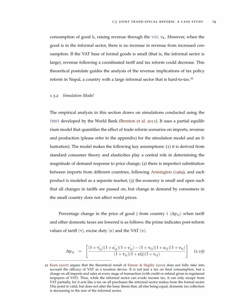
Percentage change in the price of good j from country i (∆pij) when tariff

and other domestic taxes are lowered is as follows: the prime indicates post-reform

values of tariff (τ), excise duty (e) and the VAT (v).

∆pij =

[(1+ τ

′ij)(1+ e

′ij)(1+ v

′ij) − (1+ τij)(1+ eij)(1+ vij)

(1+ τij)(1+ eij)(1+ vij)

](1.15)

22 Keen (2007) argues that the theoretical result of Emran & Stiglitz (2005) does not fully take intoaccount the efficacy of VAT as a taxation device. It is not just a tax on final consumption, but acharge on all imports and sales at every stage of transaction (with credit or refund given to registeredtaxpayers of VAT). Thus, while the informal sector can evade income tax, it can only escape fromVAT partially, for it acts like a tax on all purchases the informal sector makes from the formal sector.This point is valid, but does not alter the basic thesis that, all else being equal, domestic tax collectionis decreasing in the size of the informal sector.


Demand responds to the relative price change in three steps, as explained by

Lim & Saborowski (2010) and Brenton et al. (2011). First, shares of expenditure on

imports of a product across different exporting countries change when a particular

tariff is altered. Total imports remain the same, but if imports of Country A become

cheaper, there will be substitution away from imports from other countries. The

elasticity of substitution is calculated as follows:

[4(MA/MB)

(MA/MB)

]/

[4(PA/PB)

(PA/PB)

](1.16)

where MA, MB are the same imports from Countries A and B with prices PA, PB,

respectively.

Second, the allocation of expenditure between imports and domestically pro-

duced goods is calculated. Relative demand changes are derived from changes in

the weighted average of the price of imports, adjusted by the elasticity of substitu-

tion between domestic and foreign products. If the average price of imports falls,

there will be substitution away from domestically produced goods, but total con-

sumption stays the same. Third, when average domestic price changes, there will

be an overall demand response. Consumers demand more of the good whose price

has fallen irrespective of whether it is imported or procured locally.

By definition, the partial equilibrium model has no economy-wide, intra- or

inter-sectoral linkages. This does not pose a problem here because the purpose is

to analyze the impact of tariff and tax changes on revenue in the short-term. It is not

to judge whether policy changes are beneficial from an economy-wide perspec-

tive over the long run for which a CGE model would probably be more suitable.

However, in contrast to the tractability of partial equilibrium models, CGE models

require a complex data set, a large number of exogenously imposed parameters,

and restrictive assumptions rendering the replicability and falsifiability of results

difficult.23

23 See Taylor & Von Arnim (2007) for a critique of the CGE methodology.


1.3.3 Data

The empirical analysis uses a new data set extracted from unpublished customs

records from Nepal for the calendar year 2008. It contains 417,715 import transac-

tions. In addition to the date when the import shipment was processed, the data

set lists the value of each import in Nepali Rupees inclusive of cost, insurance and

freight (c.i.f.) and tariffs levied on that import. Customs also raise a substantial

share of additional revenue at ports of entry by levying a range of domestic taxes.

The main ones in Nepal are the excise duty and VAT, as well as the Agricultural

Reform Fee (ARF) imposed on agricultural imports from India only. A range of

other charges and taxes (para tariffs) are levied as follows: demurrage, customs

service fee, fine, special fee, Road Construction Fee, and the Local Development

Tax.24 The data set lists applied Most Favored Nation (MFN) and preferential tariff

rates set for each import at the Harmonized Commodity Description and Coding

System (HS) 8-digit level.

I check for the consistency of entries and adjust the data set as follows. All im-

port transactions worth Rs. 10,000 (approx. US$140) or less are dropped.25 Goods

entering the country under customs procedure codes which do not compete in the

local market are dropped. These are mainly diplomatic and governmental imports

that are tax-exempt. Next, I compute the applied tariff rate, applied excise duty,

and applied VAT by dividing the actual amount of such taxes collected by their re-

spective base.26 Those “applied” values that abnormally deviate from the statutory

24 As of 2011, the local development tax, road construction fee, and special fee have been phased out.

25 This excludes nearly 30 percent of the observations, which accounts for 3.2 percent of total importvalue.

26 In Nepal, excise duty is levied as a percentage of import value. VAT is paid as a percentage of thebase comprising of import value plus excise and other taxes. The Agricultural Reform Fee (ARF) islevied (in lieu of tariff) on the value of agricultural imports from India. If VAT is additionally leviedon such agricultural goods from India, it is a fixed percentage of the import value, not import valueplus the ARF.


tax rates are dropped. The cleaned data set that is ready for simulation consists of

265,194 import records spanning 4032 tariff lines from 133 economies.27

The paper also incorporates domestic production data extracted from the lat-

est quinquennial Census of Manufacturing Establishments that reports the domes-

tic sale of manufactured goods (Government of Nepal 2008). For 3,079 of the 4032

import codes, there exists matching data for domestically sold products. This al-

lows for substitution of imports by domestically produced goods when the price

of imports rises, adding to the richness of simulation results. There are, however,

two limitations. First, the latest production data are available only up to the fiscal

year 2006-07, whereas the import data straddles the fiscal years of 2007-08 and

2008-09 (that is, calendar year 2008). Second, production data covers only manu-

facturing industries. For a little less than 25 percent of the tariff lines that belong

to non-manufacturing industries, there are no data on domestic production. In the

language of the model, for a subset of imports, the substitution between imports

and domestically produced goods is perfectly inelastic.

The 133 import trading partners of Nepal in 2008 are organized in eight

groups: (1) India; (2) China, including the Tibet Autonomous Region; (3) Rest of

South Asia (Afghanistan, Bangladesh, Bhutan, Maldives, Pakistan, Sri Lanka); (4)

Northeast Asia (Japan, Republic of Korea, Hong Kong Special Administrative Re-

gion, and Taiwan); (5) Southeast Asia (Indonesia, Malaysia, Philippines, Singapore,

Thailand, Vietnam); (6) North America (Canada, Mexico, United States); (7) the Eu-

ropean Union; and (8) the Rest of the World (ROW). The baseline scenarios assume

an export substitution elasticity of 1.5, domestic substitution elasticity of 1, and

import demand elasticity of 0.5.

27 The term “economies” is used in lieu of “countries” because Nepal’s customs data treat Tibet, HongKong, and Taiwan as sources of imports that are distinct from the People’s Republic of China eventhough the three economies are (politically) part of China.


1.3.3.1 Import-based Revenue in Nepal

The structure of tariffs and tariff-based revenue in Nepal is described in this section.

Columns 3 to 6 in Table 3 show that the collected tariff and VAT rates across all

imports are just over 10.5 percent and 11 percent, respectively. When imports are

weighted by value, those rates drop to 7 and 9.9 percent, respectively. That the

applied VAT rate of above 11 percent is nearly two percentage points below the

statutory rate of 13 percent indicates the scale of average exemptions, a proxy for

discretion that the authorities exercise. For tariffs, the scale of average exemptions

is the difference between the weighted statutory tariff rate of 8.33 percent and the

applied tariff rate of 7 percent.28 Compared to just 20 years ago, the height of trade

protection has fallen considerably, although revenue generated by taxing imports

through tariffs, VAT and excise continues to be the dominant source of tax revenue

in Nepal.

After the adjustments described in the preceding section are made, the total

value of imports in 2008 is Rs. 222.19 billion.29 Table 3 shows that in 2008, Nepal

received Rs. 15.6 billion in tariff revenue, amounting to 34.3 percent of total rev-

enue derived from imports. VAT on these imports (Rs. 23.9 billion) accounted for

52.7 percent of the total import-based revenue, and the remaining 13 percent was

accounted for by excise and other taxes amounting to nearly Rs. 6 billion.

Figure 2 shows that VAT (on both imports and domestic consumption) sur-

passed customs-based revenue as the main source of tax revenue after 2004. How-

28 The extent of exemptions granted can only be assessed for products subject to ad valorem duties.Because the AVE for specific tariffs have been computed by the so-called income method of takingthe (median) applied tariff rate, there is no difference between the statutory and collected tariff ratesfor the category of imports that face specific tariffs.

29 This figure is for the calendar year 2008. Its comparison with total import figures for the fiscal year2008 deserves care. The reported total import by Nepal in the fiscal year (from July 2008 to July 2009)was Rs. 284.5 billion. In the fiscal year 2007-08 (from July 2007 to July 2008), total import was Rs.221.9 billion. The raw customs total for the calendar year 2008 is in between the figures for the twofiscal years, at Rs. 236.6 billion. After adjustment, this drops to Rs. 222.2 billion.


Figure 2: Share of Tax Revenue by Source

�

��

��

��

��

��

��

��

� ��!�"�#��$�%�&�'�(��)%��!�� '�*� ��&��$$ +��&��*�� +��*�� ,�$��*

ever, as shown in Table 4, at least 62 percent of total VAT revenue is derived from

imports.30

Table 5 shows the distribution of observations by tariff bands ranging from

zero to 80 percent for SAFTA and non-SAFTA trading partners. There is an ad-

ditional row for products (such as fuel, tobacco, alcohol and cement) that face

specific tariffs (that is, per quantity, not percentage of value). The first group com-

prises countries that generally pay a higher rate of applied MFN tariff. The second

group of countries pays preferential tariff rate under SAFTA. This group accounts

for nearly 64 percent of imports into Nepal, and is almost exclusively dominated

by India.

Several features stand out in Table 5. First, less than 15 percent of imports (by

value) are free of statutory duty. Second, nearly 36 percent of imports are subject

to “nuisance” tariffs between zero and five percent; the term indicates that at such

30 Data from the Internal Revenue Department of the Ministry of Finance of the Government of Nepalas published in Government of Nepal (2004), Government of Nepal (2009) and Government of Nepal(2010) show that VAT revenue from imports has exceeded 60 percent over the past 10 years.


low rates the cost of monitoring and collecting tariffs could outweigh the revenue

collected. Third, there are 421 observations that are subject to specific tariffs, whose

Ad Valorem Equivalent (AVE) is 26 percent. The AVE of specific tariffs is calculated

as the median applied tariff rate of all applicable imports at the HS 8-digit level

(that is, customs tariff divided by import value). Almost all the goods on which

specific tariffs are levied originate in India. These goods account for 19.2 percent

of total import value and 22.6 percent of collected tariffs.

1.3.4 Results

1.3.4.1 Coordinated Tariff and Tax Reform with Small Informal Sector

This section reports results of the impact of five reform scenarios of coordinated tar-

iff cuts and VAT consolidation. In the first scenario, statutory tariffs on all imports

are cut by 50 percent, together with a full enforcement of the VAT at the existing 13

percent.31 Full implementation means that all imports and domestically produced

goods are charged a non-discriminatory VAT rate of 13 percent with no exception.

All “other” taxes and charges including the Agricultural Reform Fee, fines and

demurrage are eliminated.32

The essence of this reform is to reduce significantly the distortionary trade tax

and recoup potential tariff losses by plugging exemptions on a much wider VAT

base. In scenario 1 of Table 6, total imports increase by 0.3 percent in value. Note

that this appears to be a small response to such a drastic cut in tariffs. However,

cuts in tariff have been accompanied by an indiscriminate application of the VAT.

This could, in some cases, raise the domestic price of the good even though the

31 Note that the statutory tariff rates are applied MFN or preferential rates. They are not bound MFNrates.

32 Nepal has already announced that it would phase out the ARF.


trade-weighted applied tariff rate drops from 7 to 4.3 percent. This suggests that

there is substitution away from domestic production.

The 50 percent cut would not “bite” if some imports were currently being

charged less than the statutory tariff rate because of discretion exercised by cus-

toms authorities, corruption, or temporary government exemptions. In scenario 1,

tariff revenues drop by 38.3 percent, as expected, from Rs. 15.6 billion to Rs. 9.6

billion. The VAT compensates for the tariff loss even when other domestic tax-

es/charges are eliminated. VAT revenue on imports increases from Rs. 23.9 billion

to Rs. 30.6 billion, and VAT revenue on domestically produced goods increases

from Rs. 10.7 billion to Rs. 13.6 billion (not shown in a disaggregated manner in

the table). Overall, this reform that cuts tariffs by half and enforces the existing

VAT ends up being more than revenue-neutral: total revenue goes up by 1 percent,

while domestic production suffers a modest loss of 0.14 percent.

In scenario 2, I apply a uniform tariff rate of five percent on all imports from

all countries and match that, again, with full implementation of the existing VAT

rate of 13 percent and elimination of all other taxes/charges. The tariff cuts are less

biting than in scenario 1, because existing tariffs that are already less than 5 percent

are increased to five percent. This affects nearly 17 percent of tariff lines, and

tariff revenue from this subset increases. However, tariff revenue from products on

which the existing tariff rate exceeds five percent is likely to decline. The net effect

of this reform on tariff revenue is a loss of 28.9 percent. When the VAT is levied

on all imports, the final decline of total tax revenue from imports is from Rs. 45.4

billion to Rs. 44.1 billion. This modest loss is more than made up for by the VAT

imposed on domestic products. Overall tax revenue from imports and domestic

sales under the second scenario increases by 2.7 percent.

In scenarios 3 and 4, the VAT rate is increased to 15 and 17 percent, respec-

tively. As expected, total revenues increase by 13.3 and 23.7 percent. In scenario 5,

I simulate another radical combination of complete full trade with no tariff on any

import, matched by a flat VAT of 17 percent on all goods. This leads to a drop in


tariff revenue from Rs. 15.6 billion to zero; however, total effect on revenue is a net

increase of 4 percent.

The message from the simulation results reported in Table 6 is that trade

taxes can be reduced without adversely affecting total government revenues by

implementing domestic taxes like VAT and excise duties effectively. In fact, if tariffs

are used mainly for revenue-raising purposes (that is, not used to protect domestic

industries) they could simply be replaced by excise taxes. Like VAT, excise taxes do

not discriminate between domestic and international sources. They also do not fall

under the purview of trade agreements, so countries under pressure to cut tariffs

can simply switch to excise. This would just be a semantic change in nomenclature.

There is, however, a powerful assumption behind the advocacy of a switch in

tax regime from tariffs to a broad-based consumption tax, namely, that countries

have the capacity to enforce a complicated system like the VAT. One of the main

arguments for reliance by poor countries on tariffs has always been that they are

easier and less costly to collect at fixed border points.

As postulated in section 2, we need a larger VAT base to raise the same level of

revenue in the presence of an informal sector. Piggott & Whalley (2001) show that

VAT expansion can reduce welfare if it encourages suppliers to go underground

to evade new taxes. The presence of the informal sector, however, may not dent

revenue collection to the extent that the theory suggests. This is because a substan-

tial share of revenue in poor countries is generated from VAT on imports which is

usually collected at the border together with tariffs. In the Nepali data for 2008, for

every rupee collected in tariff revenue, Rs. 1.7 was collected additionally in VAT

and excise duty. This point is also made by Keen (2008) that the VAT (and withhold-

ing taxes) on imports actually acts as a tax on the informal sector. While the formal

sector may claim tax credit on payments made at the border when they eventually

pay income and other taxes, the informal sector does not, thereby minimizing loss

to the exchequer.


1.3.4.2 Coordinated Tariff and Tax Reform with Large Informal Sector

In this subsection, I allow for an exogenous shrinking of the taxable production

base (Table 7), which is equivalent to the enlargement of the informal sector. In

section 2 of this paper, it was shown that the presence of a large informal sector

makes it difficult to raise revenue from domestic sources. To proxy for the informal

sector, I run the same simulations as in Table 6, but with the assumption that the

taxable domestic base has shrunk by 30 percent.

In scenario 1 presented in Table 7, the same policy simulation as in scenario

1 in Table 6 leads to a drop in overall revenue by 0.6 percent. This is because the

VAT is levied on a smaller production base (with activities going underground in

response to the commodity tax hike). In scenarios 2, 3 and 4 with a uniform tariff

of 5 percent matched by increasing rates of VAT, the net increase in total revenue

is less than in Table 6 for identical simulations. While scenario 5 raised total tax

revenue by 4 percent, as in Table 6, the increase in revenue is only 0.5 percent in

the presence of an enlarged informal sector.

Ideally, the size of the informal sector ought to respond endogenously to the

tax system. However, discussion of this is beyond the scope of this section whose

the goal is to illustrate that i) it is costly to raise taxes on a narrow base and ii)

revenue loss from a switch in trade to domestic commodity taxes is minimized

when imports form an important part of the domestic tax base. In extreme cases,

such a coordinated tariff and tax reform could merely lead to a replacement of tariff

by VAT and excise at the border. There will, however, be a substantial difference

made to production efficiency in the formal sector by switching to VAT and excise.

Furthermore, while the VAT generally only taxes the informal sector if it consumes

inputs from the taxed formal sector, this is not the case when imports are a large

part of the VAT base when it can tax informal sector sales, as well as profits of

formal sector firms (Boadway & Sato 2009).


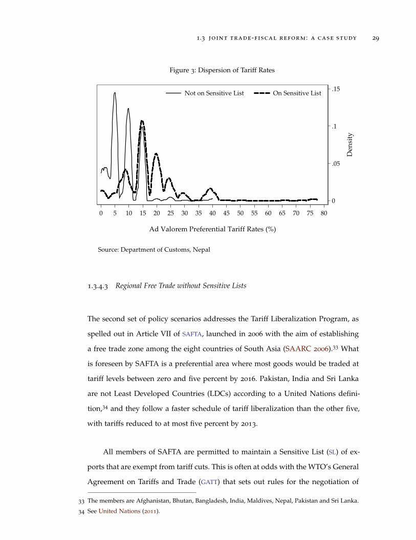
Figure 3: Dispersion of Tariff Rates

�

��

��

��

��

��

� � ��

��

��

�

�� !��"

1.3.4.3 Regional Free Trade without Sensitive Lists

The second set of policy scenarios addresses the Tariff Liberalization Program, as

spelled out in Article VII of SAFTA, launched in 2006 with the aim of establishing

a free trade zone among the eight countries of South Asia (SAARC 2006).33 What

is foreseen by SAFTA is a preferential area where most goods would be traded at

tariff levels between zero and five percent by 2016. Pakistan, India and Sri Lanka

are not Least Developed Countries (LDCs) according to a United Nations defini-

tion,34 and they follow a faster schedule of tariff liberalization than the other five,

with tariffs reduced to at most five percent by 2013.

All members of SAFTA are permitted to maintain a Sensitive List (SL) of ex-

ports that are exempt from tariff cuts. This is often at odds with the WTO’s General

Agreement on Tariffs and Trade (GATT) that sets out rules for the negotiation of

33 The members are Afghanistan, Bhutan, Bangladesh, India, Maldives, Nepal, Pakistan and Sri Lanka.

34 See United Nations (2011).


customs unions and free trade areas. Article XXIV of GATT allows regional trad-

ing arrangements to be set up as a special exception to the MFN rule if tariffs and

other barriers are eliminated for substantially all the trade. There is, however, no

agreement on what numerical share of trade constitutes “substantially all.”

Table 8 shows impacts on Nepali imports, tariff revenue, and total tax revenue

from implementing various tariff and VAT changes in relation to trade in the South

Asia region. India accounts for over 63 percent of imports and the six other South

Asian countries collectively account for less than 0.5 percent (Table 12). Thus, from

the perspective of Nepali imports, free trade in South Asia is equivalent to free

trade with India.

Scenario 1 in Table 8 applies tariffs at the agreed preferential rates with no

exemption while eliminating the Agricultural Reform Fee, and other charges like

fines and demurrage. VAT and excise are not adjusted, and tariffs on countries

outside South Asia are not changed. This modest incremental reform appears to be

roughly revenue-neutral. In other words, simply applying agreed statutory rates

on imports and eliminating tariff exemptions on imports from South Asia can

pay for the elimination of the Agricultural Reform Fee currently levied on Indian

agricultural imports. This would require no further change to the domestic tax

regime.

Scenario 2 simulates complete free trade with South Asia, but tariffs on im-

ports from the rest of the world are unchanged. Further, the existing VAT rate of

13 percent is enforced strongly on all imports and domestically produced goods.

This scenario is unfavorable to Nepal as total tax revenue drops from Rs. 60 billion

to Rs. 56.4 billion (by more than six percent). This indicates that even the full force

of a perfectly implemented VAT at the existing rate is not sufficient to recoup tariff

revenue loss of more than 62 percent (from Rs. 15.6 billion to Rs. 5.9 billion) as a

consequence of free trade with the rest of South Asia. Scenario 3 shows, however,

that a VAT of 15 percent is adequate to make up for the revenue cost of free trade

with South Asia. Net tax revenues increase by 4.5 percent.


In scenario 4, I foresee complete free trade within South Asia, enforcement

of the VAT at 15 percent, elimination of ARF and other charges, and application

of a uniform tariff of eight percent on imports from the rest of the world. This is

almost equivalent to scenario 3, except that under this scenario, applied weighted

tariff increases from 2.6 percent to 2.8 percent. In other words, scenario 3 is slightly

more protectionist, but administratively simpler because there are only two tariff

rates to enforce: zero percent for South Asian imports and eight percent for the

rest.

Scenario 5 extends SAFTA to include China, envisioning a free trade area

around Nepal that is peopled by 2.5 billion consumers. Interestingly, zero tariffs on

all Indian and Chinese imports can be compensated by the full application of the

VAT at 15 percent. Because China and India accounted for three-quarters of Nepali

imports in 2008, reducing all tariffs on them to zero reduces the trade-weighted

collected tariff (rate of protection) from seven to under two percent.

1.3.4.4 Regional Free Trade with Sensitive Lists

The Sensitive List shields products from tariff cut commitments on the basis of

self-defined national interest. Among the members of SAFTA, Nepal maintains

the longest list of sensitive products that are exempt from progressive tariff cuts

(Table 13). By 2016, only products that are not on the Sensitive List whose tariffs

will be confined to between zero and five percent.35 Of the 1295 products (at the

HS 6-digit level) on Nepal’s Sensitive List of imports from the larger South Asian

economies (India, Pakistan, Sri Lanka), more than 250 were not even imported

into the country in 2008. The average tariff level of products on the Sensitive List

is higher than those not on the list, as shown in Figure 3. For products on the

list, there is a noticeable “bunching” around the rates of 15, 20, 25 and 40 percent,

35 In South Asia, Bhutan has the shortest list, followed by India’s list for LDCs. India’s list for Pakistanand Sri Lanka is much longer.


whereas for products not on the list, the densities are higher at lower tariff rates of

five and 10 percent.

Scenario 1 in Table 9 presents the revenue baseline when there is free trade

with South Asia (with tariffs and other taxes, but not excise, eliminated). The exist-

ing pattern of VAT is unchanged, as are tariffs on the rest of the world. Predictably,

with 63 percent of total imports rendered duty-free, tariff revenues collapse by

nearly 62 percent, and overall government revenues are reduced by 22.4 percent.

Trade-weighted average applied tariff rate also drops from seven to 2.6 percent.

The difference with scenario 2 in Table 6 is that in the latter, tariff cuts are accom-

panied by full enforcement of the existing VAT rate, leading to an overall revenue

decline of only 6.1 percent.

Scenario 2 repeats the previous simulation, but allows no tariff cuts on prod-

ucts on the government’s existing Sensitive List. Tariff is not reduced to zero on

1092 products (but other taxes including the ARF are eliminated). This limits rev-

enue loss from imports to only about 10 percent, and when revenue from domestic

production is allowed for, the government revenue drops by only 7.9 percent. The

existing Sensitive List, therefore, protects revenue by nearly 15 percentage points.

The down-side of this is that the trade-weighted average applied tariff rate has

only dropped by 0.9 percentage points, from the pre-reform seven percent to the

post-reform 6.1 percent. This suggests that while Nepal has signed up for freer

trade, it is exhibiting anxiety about the consequences by using a lengthy Sensitive

List that is legally sanctioned but operationally detrimental to the ethos of freer

trade.

In scenario 3, I devise an alternative Sensitive List with 1096 products at the

HS 8-digit level (same number as the government’s existing list) with the sole ob-

jective of minimizing revenue loss from intra-regional free trade. The alternative

Sensitive List is prepared by simulating unconditional free trade, and looking at

final revenue changes at the product level subsequent to the three channels of


adjustment described in Section 3. Products that recorded the highest losses are

sorted and 1096 of them put on the Sensitive List. This preserves revenues by an

additional 3.4 percentage points over and above the government’s list. Indeed, tar-

iff revenues increase under this scenario; it is only after accounting for the loss of

other taxes that total revenue falls from Rs. 60 billion to Rs. 57.3 billion. The conse-

quence of applying such a conservative Sensitive List is that there is no meaningful

reduction in distortion from trade taxes as a result of intra-regional free trade. The

trade-weighted average applied tariff rate stays unchanged at seven percent.

Scenarios 2 and 3 do not lead to as big a revenue loss as under complete

intra-regional free trade because the Sensitive Lists are devised by counting the

number of tariff lines. This approach is irrespective of the magnitude of the share

of individual imports, and all high value tariff lines can be shielded from cuts.

Indeed, the government’s Sensitive List covers 50 percent of all imports, and my

alternative list covers 84 percent of imports. This suggests that if the purpose of a

regional free trade agreement is to foster regional trade, either the Sensitive Lists

ought to be scrapped, or capped by value, in line with Article XXIV of GATT that

permits an exception to the WTO’s sacrosanct MFN principle (GATT Article I) only

if regional trade blocs cover substantially all the trade among members.

Next, I examine the revenue consequences of free trade with South Asia when

Nepal is permitted to design a Sensitive List that cumulatively accounts for 5,

10, and 20 percent of trade value. In other words, “substantially all the trade” is

interpreted as 95, 90, and 80 percent of total imports, respectively.

Scenario 4 caps the cumulative import value of products in the Sensitive List

at 20 percent. This list was created by adding the share of revenue changes normal-

ized by the import value of each product from the South Asia region. Although this

list is longer, in terms of the number of tariff lines shielded, than in the preceding

two scenarios, capping the value at 20 percent frees up many high-value import

categories that are now subject to tariff cuts. Overall revenue in this case decreases

by 10.4 percent. Scenario 5 caps import value at 10 percent, leading to overall rev-


enue loss of 13.8 percent. Scenario 6 caps the Sensitive List at five percent of import

value, leading to a loss in revenue of 18.1 percent (Rs. 11 billion), which is more

than under complete intra-regional free trade (scenario 1). In these simulations, the

weighted average rate of collected tariffs halve, from 7 to 3.5 percent.

The simulation results reported in Table 9 illustrate that the design of Sensi-

tive Lists is crucial, with potential for either fostering or frustrating the objective

of regional free trade. Sensitive Lists that are carved out by counting tariff lines ap-

pear to undermine the objective of intra-regional free trade more than when such

lists shield products by value. In all cases, revenue losses are big, but as shown in

Table 8, these can be recouped through reforms to the domestic tax regime, espe-

cially a full and effective implementation of the VAT at existing or slightly higher

rates.

1.3.5 Robustness

In this section, two major simulations from Tables 6 and 8 are re-run allowing for

higher elasticities. Scenario 1 of Table 10 uses default elasticities and is identical to

scenario 1 of Table 6 where the reform consists of a 50 percent cut in statutory tar-

iffs on all imports from all countries matched by an effective 13 percent VAT on all

goods. Scenario 2 repeats this simulation with higher elasticities: three for export

substitution and two for domestic substitution, with demand elasticity applied at

the disaggregated product level using the estimates of Kee et al. (2008). Scenario 3

repeats scenario 2, with an additional increase in only the exporter substitutability

parameter from three to six.

The results in scenarios 2 and 3, compared to scenario 1, confirm that the

responsiveness of imports to relative price changes is increasing in substitutability.

Compared to the default case, imports increase by two percentage points, which

reduces the loss in tariff revenue by 5.8 percentage points. Overall tax revenue

increases by 3.3 percentage points when elasticities increase.


Scenarios 4 to 6 simulate the revenue consequences – under varying sets of

elasticities – for free trade under SAFTA with a Sensitive List that I create to cap

imports under exemption to not exceed 10 percent of total import value from South

Asia. This reform is closer to the spirit of freer regional trade, but it leads to greater

revenue losses. Consistent with the previous set of simulations, revenue losses are

decreasing in elasticity: the higher the degree of substitution allowed in response

to import and domestic prices, the smaller the decline in revenue.

Note a nuanced change between scenarios 2 and 3 versus scenarios 5 and 6

in Table 10. The difference between scenarios 2 and 3 and between 5 and 6 lies

only in the exporter substitution elasticity. In the case of coordinated tax and tariff

reform, all tariffs are cut and domestic tax is enforced on all goods. If there was

no exemption on any good, this reform would not have triggered any substitu-

tion among exporters. Any increase in imports would be a result of final domestic

price changes leading to increased demand for all products irrespective of origin.

Because the existing VAT is not applied uniformly, the reform does lead to rela-

tive price changes, permitting some substitutability in imports by destination. The

overall effect is that higher exporter substitutability (everything else being equal)

leads to greater import response, tariff revenue, and total tax collection.

In scenarios 4, 5, and 6, however, the reform entails a radical cut in tariffs on

South Asian imports only. When all elasticities increase in tandem, the net loss of

revenue is less than under the default case. This is consistent with previous simu-

lations where higher elasticities led to greater substitutability and import demand

in response to overall price fall. However, when I increase only the exporter substi-

tutability elasticity in scenario 6, overall tariff and tax revenues decrease by more

than in scenario 5. The reason for this is that as a result of tariff elimination within

South Asia, there is substitution of imports away from the rest of the world. But

there is no tariff earned on South Asian imports under free trade. Because tariffs

are part of the VAT base, elimination of tariffs leads to a further fall in revenue

from VAT.


1.4 related issues in tariff reform

1.4.1 Change in Domestic Prices and Production

Together with the revenue consequences, TRIST simulations indicate the extent

to which domestic production is substituted for by imports when the latter be-

come cheaper as a result of tariff cuts. Products are clustered by sector at the

International Standard Industrial Classification (ISIC) 3-digit level. In my data set,

domestic production figures are only available for broadly-defined manufacturing

industries. Because inter-sectoral cross-linkages are not incorporated in this model,

the projected change in average prices and production apply to each sector only.

Table 11 shows the value of domestic sales before and after Nepal applies zero

tariff on all imports from South Asia without and with exemptions (as in scenarios

1 and 2 of Table 9). Predictably, the transport and motor vehicle sectors undergo

the biggest change as a result of reforms because these products attract some of

the highest rates of tariff at present. Note that because high rates of excise duty

and VAT are still applied on some of these products, average prices do not fall

dramatically. For example, the rate of protection of the motor vehicle sector falls

by 16 percentage points, but still remains at over 12 percent, unlike several other

sectors where the rate of protection falls below three percent.

Table 11 disaggregates tariff revenue at the sectoral level. Among the top 10

sectors listed, the loss of tariff revenue is least pronounced in apparel and animal

rearing sectors (ISIC 12 and 181). In the remaining sectors, tariff revenues fall by

between 46 and 99 percent. If the government’s highly liberal Sensitive List shields

some of the products which are anticipated to experience big revenue changes (for

example, motor vehicles), the picture of domestic price and production change

would alter. This is shown in the bottom half of the same table. Transport equip-

ment and motor vehicles are protected from tariff cuts in the government’s existing

Sensitive List, so modest changes in domestic sales occur in primary sectors (ani-

1.4 related issues in tariff reform 37

mal rearing, mining, forestry) and basic manufacturing industries. Change in the

level of protection as well as tariff revenues is also less severe than in the case when

no product is shielded from tariff cuts.

1.4.2 Collected and Statutory Rates

Pritchett & Sethi (1994) found for some developing countries36 that collected (ap-

plied) tariff rates are only weakly correlated with statutory rates and that the for-

mer decrease non-linearly as the latter rise. This reflects the problem of granting

tariff exemptions discretionarily, and opening up opportunities for graft. Revisit-

ing Nepal’s import data for 2008, I find that the issue of a discrepancy between

statutory and collected tariff rates is less important for Nepal. This is perhaps the

effect of the sustained tariff reforms over the past 20 years that have focused on

lowering the average rates as well as reducing the number of tariff bands through

policy reforms supported by international organizations like the World Bank, IMF,

and the World Trade Organization (WTO).

Table 14 lists the mean rate of collected tariff and its dispersion at selected

statutory rates. However, except at the highest rate of 80 percent, applied tariff

rates are only marginally less than statutory rates, indicating a high degree of

compliance on average. When individual import transactions are parsed, however,

the degree of discrepancy appears wider. Figure 4 depicts this graphically where

23 percent of import transactions (out of 256,971) paid tariffs that did not match the

statutory tariff rate. If the collected tariff rate is less than the statutory rate, it could

mean either of the following: i) tariffs were legally sacrificed as part of a conscious

government decision, such as import duty rebates as part of an export promotion

strategy, ii) other para-tariffs have been introduced in lieu of, or on top of, tariffs,

such as the Agricultural Reform Fee, or iii) there is malpractice in the customs

administration where authorities exercise improper discretion and exempt certain

36 Their data are for Jamaica (1991), Kenya (1987) and Pakistan (1991).


Figure 4: Statutory and Collected Tariff Rates

�

��

��

��

��

��

�

� ��

��

�

�� !�� "#� �� $� ��%��&� �� "#� �� $� ��'��&� ��

imports from tariffs and taxes. In a negligible number of cases, collected tariff rates

are actually higher than the ad valorem statutory rates.37

If all importers paid the statutory rate, it would be a perfect predictor of the

collected tariff rate in a simple regression of applied tariff on statutory tariff. In

Nepal, the explanatory power (R2) of the latter on the former is higher (0.82) than

that found by Pritchett & Sethi (1994). Further, a spline regression that allows

for different slopes for two subsets of tariff rates (below and above 25 percent),

and a quadratic regression of applied rate on statutory rate and its squared value

demonstrate a high explanatory power, confirming that the correlation between

statutory and collected tariff rates for Nepal is strong, but collected tariff rates do

decline as statutory rates rise.

37 This could be a result of specific decrees, or that these imports could be akin to personal effectsthat are generally charged a high tariff but no VAT. In 2008, there were 36 such items, 30 of whichbelonged to HS 3706 (Cinematography film). Note also that records corresponding to the high statu-tory rate of 80 percent applying largely to motor vehicles show that a number of exemptions weregranted to parties that were neither government nor diplomatic establishments.

1.5 conclusion 39

Related to this is the issue of smuggling and under-invoicing. If statutory tariff

rates and other border taxes are higher than the cost of smuggling, they provide

incentives for smugglers to evade high tariffs. Since smuggling is not costless (it

takes resources to arrange for successful smuggling, and face the law if caught),

lowering of ad valorem tariffs decreases the incentives for smuggling.

Importers also have an incentive to collude with exporters to under-invoice

their import value in order to pay less tariffs when duties are ad valorem. An

intuitive solution for this is to levy specific tariffs, and not ad valorem, but specific

tariffs have their own complications. The more important point is that both the

problem of under-invoicing and smuggling are partly triggered by a cascading

tariff structure where final goods attract high tariffs and intermediate goods attract

low tariffs. Lowering of all tariffs could therefore encourage more goods to flow

through formal channels, increasing tariff revenue.

1.5 conclusion

Tariffs have historically served the dual purpose of raising government revenue

and protecting domestic producers. This was clearly seen in many developing

countries when they experimented with import substitution policies behind high

tariff walls in the post-war period.38 In recent decades, the economic paradigm

has shifted decisively towards greater liberalization, diminishing the protective

function of tariffs. In the poorest countries, however, the revenue-raising role of

tariffs remains important. The short-term concern over loss of revenue, therefore,

has often stymied necessary trade and fiscal reforms.

38 In the 19th century, tariffs were a major issue in the rich countries of the day as well. With no incometaxes, and the popularly known Export Clause of the Constitution banning the levying of exportduty, the United States relied heavily on tariffs. From South Carolina’s Ordinance of Nullification(of tariffs) in 1832 that triggered a crisis over federal authority under President Jackson to the GreatTariff Debate of 1888, tariffs were a divisive political issue (Irwin 1997). In Britain, the repealing oftariffs on imported grain (Corn Laws) in 1846 by Prime Minister Robert Peel split the Tory Party andbegan a brief era of freer trade.


An ideal tax system raises revenue to fund socially sanctioned government

expenditures in ways that are administratively and politically feasible while pro-

moting equity and efficiency (Burgess & Stern 1993). As countries become richer,

they move towards this ideal by relying more on direct sources of taxation on per-

sonal income. Because of capacity constraints and high enforcement costs, however,

developing countries focus on narrow tax bases that not only distort incentives and

resource allocation, but also raise revenue that is inadequate to fund development

needs.39

This paper contributes to the debate on ways to reform trade practices without

adversely affecting the fiscal base of poor countries. Cross-country evidence from

35 low-income countries also shows that as countries move away from trade-based

taxes, they manage to partially offset trade-based revenue losses with domestic

sources of taxes. That the presence of VAT is not more strongly associated with rev-

enue recovery is a surprise because this is not what the simulations suggest. This

can only be resolved if we acknowledge the great heterogeneity in VAT regimes

across countries, with efficacy dependent on factors beyond the ad valorem rate,

such as the size of the informal sector, product coverage of the value-added tax,

systems of tax refund, and the capacity of tax administrations.

Using actual data on import value, tariffs, and up to ten domestic taxes on

more than 400,000 import transactions from Nepal, I develop scenarios in which

tariffs can be cut with the least impact on total revenue. This requires eliminating

widespread exemptions and an effective implementation of domestic taxes such as

VAT and excise spanning a widened base. The degree of informality and the hard-

to-tax sectors complicate tax replacement, but a measured approach to reducing

tariffs and expanding consumption taxes could minimize adjustment costs. In the

39 Consider a hypothetical scenario where a typical poor country raises taxes of around 12 percent ofGDP. It raises another 3 percent of GDP in non-tax revenue. Add to it a fiscal deficit of 5 percent ofGDP. It then has to meet its immense development challenges like poverty alleviation with a resourceenvelope of around 20 percent of GDP. (Note that the interest burden on annual borrowing alone, at8 percent, would add 0.4 percent of GDP in subsequent years.)

1.5 conclusion 41

case of regional free trade, Sensitive Lists can be crafted judiciously to minimize

the strain on revenue.

The overarching policy lesson is that in countries undertaking trade reform,

it is necessary to identify alternative sources of revenue ex ante. This steers de-

veloping countries towards strengthening their domestic tax system rather than

resisting reforms. The use of partial (or general) equilibrium models, under sensi-

ble assumptions, produces estimates that assuage fears about the scale of loss of

revenue and production. The models contribute to evidence-based policy making

on the parameters of reform such as tariff-cutting formulae, schedules of prod-

ucts to exempt, and sectors to help temporarily. This is a period unprecedented in

world history when countries at all income levels are engaged in simultaneous trade

negotiations at the multilateral, regional, and bilateral levels. The utility of swift,

time-sensitive analyses of trade adjustment costs, as attempted in this paper, could

therefore be high.

references

Arellano, M. & Bond, S. (1991), ‘Some tests of specification for panel data: MonteCarlo evidence and an application to employment equations’, The Review of Eco-nomic Studies 58(2), 277.

Arellano, M. & Bover, O. (1995), ‘Another look at the instrumental variable estima-tion of error-components models’, Journal of Econometrics 68(1), 29–51.

Armington, P. (1969), ‘A theory of demand for products differentiated by place ofproduction’, IMF Staff Papers 16, 159–76.

Baunsgaard, T. & Keen, M. (2005), ‘Tax revenue and (or?) trade liberalization’, IMFStaff Papers No. 112 (WP/05).

Baunsgaard, T. & Keen, M. (2010), ‘Tax revenue and (or?) trade liberalization’,Journal of Public Economics 94(9-10), 563 – 577.

Bertrand, T. & Vanek, J. (1971), ‘The theory of tariffs, taxes, and subsidies: someaspects of the second best’, The American Economic Review 61(5), 925–931.

Bhagwati, J. & Srinivasan, T. (1999), ‘Outward-orientation and development: arerevisionists right?’, Yale University Economic Growth Center Discussion Paper No.806.

Blundell, R. & Bond, S. (2000), ‘GMM estimation with persistent panel data: anapplication to production functions’, Econometric Reviews 19(3), 321–340.

Boadway, R. & Sato, M. (2009), ‘Optimal tax design and enforcement with an infor-mal sector’, American Economic Journal: Economic Policy 1(1), 1–27.

Bolt, K., Matete, M. & Clemens, M. (2002), ‘Manual for Calculating Ad-justed Net Savings’. World Bank Draft. Accessed October 21, 2011

<http://go.worldbank.org/VLJHBLZP71>.

Brenton, P., Saborowski, C., Staritz, C. & Von Uexkull, E. (2011), ‘Assessing theadjustment implications of trade policy changes using the Tariff Reform ImpactSimulation Tool (TRIST)’, World Trade Review 10(02), 249–276.

Buehn, A. & Schneider, F. (2007), ‘Shadow economies and corruption all over theworld: revised estimates for 120 countries’, Economics: The Open-Access, Open-Assessment E-Journal 1(2007-9).

Buffie, E. (2001), Trade Policy in Developing Countries, Cambridge University Press:Cambridge.

Burgess, R. & Stern, N. (1993), ‘Taxation and development’, Journal of EconomicLiterature 31(2), 762–830.

Cockburn, J. (2006), ‘Trade liberalisation and poverty in Nepal: a computable gen-eral equilibrium analysis’, Globalisation and Poverty: Channels and Policy Responses,Routledge, New York pp. 171–94.

42

Corden, W. (1997), Trade Policy and Economic Welfare, Clarendon Press: Oxford.

Dixit, A. (1985), ‘Tax policy in open economies’, Handbook of Public Economics 1, 313–374.

Emran, M. & Stiglitz, J. (2005), ‘On selective indirect tax reform in developingcountries’, Journal of Public Economics 89(4), 599–623.

Ernst & Young (2008), The 2008 Worldwide VAT and GST Guide, EYGM Limited.

Falvey, R. (1994), ‘Revenue enhancing tariff reform’, Review of World Economics130(1), 175–190.

Government of Nepal (2004), Annual Report of the Internal Revenue Repartment 2003-04, Vol. 1, Ministry of Finance: Kathmandu.

Government of Nepal (2008), Census of Manufacturing Establishments 2006-07, Cen-tral Bureau of Statistics, National Planning Commission Secretariat: Kathmandu.



Government of Nepal (2011), Economic Survey of Fiscal Year 2010-11, Vol. 1, Ministryof Finance: Kathmandu.

Greenaway, D. & Milner, C. (1991), ‘Fiscal dependence on trade taxes and tradepolicy reform’, The Journal of Development Studies 27(3), 95–132.

Hatta, T. (1977), ‘A theory of piecemeal policy recommendations’, The Review ofEconomic Studies 44(1), 1–21.

Irwin, D. (1997), ‘Higher tariffs, lower revenues? Analyzing the fiscal aspects of the"Great Tariff Debate of 1888"’, NBER Working Papers No. 6239.

Kee, H., Nicita, A. & Olarreaga, M. (2008), ‘Import demand elasticities and tradedistortions’, The Review of Economics and Statistics 90(4), 666–682.

Keen, M. (2007), ‘VAT attacks!’, International Tax and Public Finance 14(4), 365–381.

Keen, M. (2008), ‘VAT, tariffs, and withholding: Border taxes and informality indeveloping countries’, Journal of Public Economics 92(10-11), 1892 – 1906.

Keen, M. & Ligthart, J. (1999), ‘Coordinating tariff reduction and domestic taxreform’, IMF Working Paper No. 93.

Keen, M. & Lockwood, B. (2010), ‘The value added tax: Its causes and conse-quences’, Journal of Development Economics 92(2), 138–151.

Khanal, D. R. (2006), ‘Public finance implications of trade reforms: Nepal casestudy’. UNDP Regional Center (Colombo) Draft.

43

Krever, R., ed. (2008), VAT in Africa, Pretoria University Law Press: Pretoria.

Lewis, S. R. (1963), ‘Government revenue from foreign trade: an international com-parison’, The Manchester School 31(1), 39–46.

Lim, J. & Saborowski, C. (2010), ‘Estimates of trade-related adjustment costs inSyria’, Journal of Policy Modeling 32(6), 843–864.

Lipsey, R. & Lancaster, K. (1956), ‘The general theory of second best’, The Review ofEconomic Studies 24(1), 11–32.

Lloyd, P. (1974), ‘A more general theory of price distortions in open economies’,Journal of International Economics 4(4), 365–386.

Meade, J. (1955), Trade and Welfare, Vol. 2, Oxford University Press: Oxford.

Munk, K. (2008), ‘Tax-tariff reform with costs of tax administration’, InternationalTax and Public Finance 15(6), 647–667.

Nickell, S. (1981), ‘Biases in dynamic models with fixed effects’, Econometrica: Jour-nal of the Econometric Society pp. 1417–1426.

Piggott, J. & Whalley, J. (2001), ‘VAT base broadening, self supply, and the InformalSector’, The American Economic Review 91(4), pp. 1084–1094.

Pritchett, L. & Sethi, G. (1994), ‘Tariff rates, tariff revenue, and tariff reform: somenew facts’, The World Bank Economic Review 8(1), 1.

Rodrik, D. (1998), ‘Why do more open economies have bigger governments?’, Jour-nal of Political Economy 106(5), 997–1032.

Roodman, D. (2009), ‘How to do xtabond2: an introduction to difference and sys-tem GMM in Stata’, Stata Journal 9(1), 86–136.

Ross, M. (2001), ‘Does oil hinder democracy?’, World Politics 53(3), 325–361.

SAARC (2006), Agreement on South Asian Free Trade Area (SAFTA), SAARCSecretariat: Kathmandu. Accessed December 2, 2011 <http://www.saarc-sec.org/userfiles/saftaagreement.pdf>.

Stewart, D. (1755), ‘The Collected Works of Dugald Stewart’, Electronic TextCenter of the University of Virginia Library . Accessed October 26, 2011

<http://etext.virginia.edu/toc/modeng/public/stesmit.html>.

Tanzi, V., Barreix, A. & Villela, L., eds (2008), Taxation and Latin American Integration,David Rockefeller Center for Latin American Studies and the Inter-AmericanDevelopment Bank.

Taylor, L. & Von Arnim, R. (2007), Modelling the impact of trade liberalisation: A cri-tique of computable general equilibrium models, Oxfam International.

44

Turunen-Red, A. & Woodland, A. (1993), Multilateral reforms of tariffs withouttransfer compensation, in H. Herberg & V. L. Ngo, eds, ‘Trade, Welfare, andEconomic Policies: Essays in Honor of Murray C. Kemp.’, Vol. 145, University ofMichigan Press: Ann Arbor, p. 166.

United Nations (2011), ‘List of Least Developed Countries’. Accessed September12, 2011 <http://www.unohrlls.org/en/ldc/25>.

Waldauer, C., Zahka, W. & Pal, S. (1996), ‘Kautilya’s Arthashastra: a neglectedprecursor to classical economics’, Indian Economic Review XXXI(1), 101–108.

World Bank (2011a), Doing Business, World Bank: Washington, D.C. Accessed Oc-tober 21, 2011 <http://www.doingbusiness.org>.

45

A P P E N D I X

1.a how the model in trist works

This illustration simplifies Brenton et al. (2011) to a case where there are only

three exporting countries (a, b, c), one exportable product (j), and an importing

home country (h). (The real world simulations in this paper involved 133 exporting

economies and 4032 products.) Existing imports from each country are multiplied

by the price change (∆pij) from equation 1.15, and adjusted by the elasticity of

substitution (σES) between imports. Total imports∑n qij = (qaj + qbj + qcj) are

held constant to isolate the substitution effect. Total import from each country after

price change and substitution is:

qESij = (1+ σES∆pij) ∗ qij.∑n qij∑

n(1+ σES∆pij) ∗ qij

(1.17)

Second, price change in imports relative to domestic price affects the allo-

cation of expenditure between imports and domestically produced goods. As a

result of the reform, the change in the weighted average price of imports (4Pj) is

the change in each price multiplied by that import’s share of total imports:

4Pj =∑n

[qij∑n qij

∗∆pij]

(1.18)

Total consumption (QD) at home consists of imports from the three countries

and domestic production. So, QD = qhj +∑n qij. Given that the elasticity of

substitution between imports and domestic good is σDS, the import of each good

after domestic substitution is:

qDSij = (1+ σDS4Pj) ∗ qESij .QD∑

n(1+ σDS4Pj) ∗ qESij

(1.19)

47


Third, the weighted average price of imports is adjusted by the share of im-

ports in total consumption. Because the price of domestically produced import-

competing product has not altered, the average change in the domestic price of

good j is deflated by the share of imports in total domestic consumption. If there is

no domestic production, the whole change in price as a result of tariff cut is passed

on to domestic consumers.

4P̃j =∑n

[∑n qij

QD4Pj

](1.20)

In response to domestic price change (4P̃j), consumers now allocate their

budget to imports and home products. Given the price elasticity of demand (σP),

total demand (QD′) for good j supplied by each of the three exporting nations and

domestic producers is:

QD′

= (1+ σP4P̃j) ∗ qDSij (1.21)

These steps are shown numerically in Table 2 with a hypothetical example, as

follows.

A product is imported from Countries A and B valued at 100 and 200 units,

respectively. The importing country levies a tariff of 30 percent, VAT of 10 percent,

and an excise duty of 5 percent (not shown). Suppose, as a result of a free trade

agreement with Country B, the tariff on imports from that country is dropped to

zero percent. The ratio of old domestic to world price for the same product from

Country B drops from 1.50 to 1.16. The import from Country A sees no change

in price because neither its tariff nor domestic taxes have altered. Because the

price of the good from Country B has dropped by 23.1 percent, imports from that

country rise. By how much depends on the exporter substitutability elasticity. At

the default value of 1.5, imports from Country B rise from 200 to 218.8, and those

from Country A fall from 100 to 81.3, keeping the pre-reform import volume intact.

1.A how the model in trist works 49

Because Country B’s share in the home country’s import of the product is

two-thirds, the weighted drop in the import price is 15.4 percent. Now, there is

substitution away from domestically produced goods towards imports from Coun-

try B as well as Country A. The exact magnitude of this shift depends, again, on

the elasticity of domestic substitution. At the default value of 1, the value of im-

ports from Country B rises to 228.9 and from Country A rises to 85 whereas home

production falls from 150 to 136.

Finally, because domestically produced goods meet only one-third of total

consumption needs at home, the weighted average domestic price of the good

falls by 10.3 percent as a result of the 23.1 percent drop in the price of the import

from a country that contributes to 45 percent of demand at home. In response, at

the assumed price elasticity of 0.5, demand for imports from all three suppliers

increases, from 228.9 to 240.7 in Country B, from 85 to 89.4 in Country A, and

from 136 to 143 at home. After the reform, total consumption increases from 450 to

473.1. Among the suppliers, Country B (on whose product tariff was cut) benefits

the most.

50

co

or

din

at

in

gt

ax

re

fo

rm

s:c

an

lo

st

ta

rif

fs

be

re

co

up

ed

?

Table 2: Illustration of Price and Demand Response in TRISTImport from Country A Import from Country B Domestic Production

Price changeInitial tariff (%) 30 30New tariff (%) 30 0VAT (%) 10 10Initial domestic to world price ratio 1.50 1.50

New domestic to world price ratio 1.50 1.16

Change in import price (%) 0.0 -23.1

Import response in three steps1. Exporter substitutionInitial product value 100 200Price change (%) 0.0 -23.1Intermediate step 100.0 269.2Value after exporter substitution 81.3 218.82. Domestic substitutionNew product value 81.3 218.8 150Price change (%) 0.0 -23.1 .Average domestic price change of imports -15.4 -15.4 0Intermediate step 93.8 252.4 150.0Value after domestic substitution 85.0 228.9 136.03. DemandLatest product value 85.0 228.9 136.0Average domestic price change of imports (%) -15.4 -15.4 .Average domestic price change (%) -10.3 -10.3 -10.3Final demand at home 89.4 240.7 143.0

1.B additional tables 51

1.b additional tables

Table 3: Tariff Rates and Import-based Revenue in Nepal, 2008

Statutory Collected Excise Value-added Othertariff tariff duty tax taxes

Revenue (billions of Rupees) 18.5 15.6 3.0 23.9 2.9Share of total tax revenue (%) 34.28 6.58 52.73 6.41

Simple average of tariff/tax rates (%) 11.42 10.54 0.58 11.03 1.89

Weighted average of tariff/tax rates (%) 8.33 7.00 1.26 9.94 1.31

Source: Unpublished data from the Department of Customs, Nepal

Table 4: VAT Collected on Imports, 2005-2010

2005-06 2006-07 2007-08 2008-09 2009-10

Revenue from VAT (billions of Rupees) 21.61 26.10 29.82 39.70 54.92Collected on imports 13.46 16.46 19.01 25.78 34.54Collected on domestic consumption 8.15 9.63 10.81 13.92 20.38VAT Revenue from imports (%) 62.29 63.09 63.75 64.94 62.89

Source: Government of Nepal (2010)

Table 5: Tariff Revenue by Band, 2008

Non-SAFTABand Observations Import Value Share Collected Tariff Statutory Tariff(%) (%) (%) (%)

a. Zero 1397 16.2 7.3 0.1 0.1b. 0 to 5 3795 34.0 15.3 6.5 5.6c. 5 to 15 4990 21.2 9.5 15.7 13.8d. 15 to 30 1689 5.8 2.6 8.2 7.1e. 30 to 80 447 1.9 0.9 7.2 6.5f. Specific (AVE) 162 1.2 0.6 0.9 1.3

SAFTAa. Zero 609 15.8 7.1 0.0 0.0b. 0 to 5 3491 45.9 20.7 10.9 9.5c. 5 to 15 5690 25.2 11.3 9.7 14.1d. 15 to 30 1424 7.5 3.4 6.1 9.5e. 30 to 80 376 6.2 2.8 13.0 15.1f. Specific (AVE) 259 41.3 18.6 21.7 17.5Total 24329 222.1 100.0 100.0 100.0

Note: Import (in billions of Rupees) from 133 partners across 4032 tariff lines.

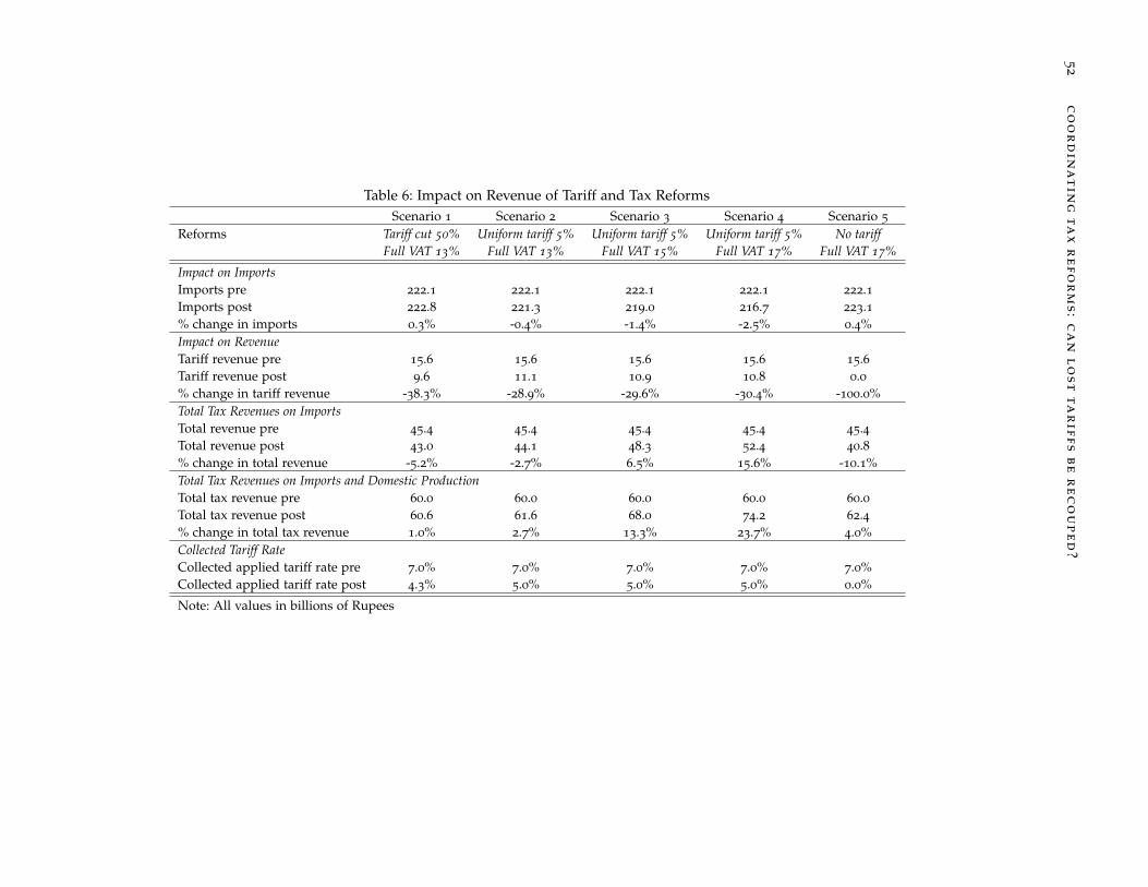
52

co

or

din

at

in

gt

ax

re

fo

rm

s:c

an

lo

st

ta

rif

fs

be

re

co

up

ed

?

Table 6: Impact on Revenue of Tariff and Tax ReformsScenario 1 Scenario 2 Scenario 3 Scenario 4 Scenario 5

Reforms Tariff cut 50% Uniform tariff 5% Uniform tariff 5% Uniform tariff 5% No tariffFull VAT 13% Full VAT 13% Full VAT 15% Full VAT 17% Full VAT 17%

Impact on ImportsImports pre 222.1 222.1 222.1 222.1 222.1Imports post 222.8 221.3 219.0 216.7 223.1% change in imports 0.3% -0.4% -1.4% -2.5% 0.4%Impact on RevenueTariff revenue pre 15.6 15.6 15.6 15.6 15.6Tariff revenue post 9.6 11.1 10.9 10.8 0.0% change in tariff revenue -38.3% -28.9% -29.6% -30.4% -100.0%Total Tax Revenues on ImportsTotal revenue pre 45.4 45.4 45.4 45.4 45.4Total revenue post 43.0 44.1 48.3 52.4 40.8% change in total revenue -5.2% -2.7% 6.5% 15.6% -10.1%Total Tax Revenues on Imports and Domestic ProductionTotal tax revenue pre 60.0 60.0 60.0 60.0 60.0Total tax revenue post 60.6 61.6 68.0 74.2 62.4% change in total tax revenue 1.0% 2.7% 13.3% 23.7% 4.0%Collected Tariff RateCollected applied tariff rate pre 7.0% 7.0% 7.0% 7.0% 7.0%Collected applied tariff rate post 4.3% 5.0% 5.0% 5.0% 0.0%

Note: All values in billions of Rupees

1.Ba

dd

it

io

na

lt

ab

le

s5

3

Table 7: Impact on Revenue of Tariff and Tax Reforms with an Informal SectorScenario 6 Scenario 7 Scenario 8 Scenario 9 Scenario 10

Reforms Tariff cut 50% Uniform tariff 5% Uniform tariff 5% Uniform tariff 5% No tariffFull VAT 13% Full VAT 13% Full VAT 15% Full VAT 17% Full VAT 17%

Impact on ImportsImports pre 222.1 222.1 222.1 222.1 222.1Imports post 222.8 221.3 219.1 216.8 223.1% change in imports 0.3% -0.4% -1.4% -2.4% 0.4%Impact on RevenueTariff revenue pre 15.6 15.6 15.6 15.6 15.6Tariff revenue post 9.6 11.1 11.0 10.8 0.0% change in tariff revenue -38.3% -28.9% -29.6% -30.3% -100.0%Total Tax Revenues on ImportsTotal revenue pre 45.4 45.4 45.4 45.4 45.4Total revenue post 43.0 44.1 48.4 52.5 40.8% change in total revenue -5.2% -2.7% 6.6% 15.6% -10.2%Total Tax Revenues on Imports and Domestic ProductionTotal tax revenue pre 55.6 55.6 55.6 55.6 55.6Total tax revenue post 55.3 56.4 62.1 67.7 55.9% change in total tax revenue -0.6% 1.4% 11.7% 21.8% 0.5%Collected Tariff RateCollected applied tariff rate pre 7.0% 7.0% 7.0% 7.0% 7.0%Collected applied tariff rate post 4.3% 5.0% 5.0% 5.0% 0.0%


54

co

or

din

at

in

gt

ax

re

fo

rm

s:c

an

lo

st

ta

rif

fs

be

re

co

up

ed

?

Table 8: Impact on Revenue of Regional Free TradeScenario 1 Scenario 2 Scenario 3 Scenario 4 Scenario 5

Reforms Stat. tariff Zero tariff Zero tariff Zero tariff SAFTA and China zero tariffNo ARF No ARF No ARF Uniform 8% on ROW Uniform 8% on ROW

Existing VAT Full VAT 13% Full VAT 15% Full VAT 15% Full VAT 15%

Impact on ImportsImports pre 222.1 222.1 222.1 222.1 222.1Imports post 222.4 224.5 222.3 221.6 222.7% change in imports 0.1% 1.1% 0.1% -0.2% 0.2%Impact on RevenueTariff revenue pre 15.6 15.6 15.6 15.6 15.6Tariff revenue post 18.0 5.9 5.8 6.1 4.3% change in tariff revenue 15.7% -62.1% -62.5% -60.5% -72.3%Total Tax Revenues on ImportsTotal revenue pre 45.4 45.4 45.4 45.4 45.4Total revenue post 45.3 38.9 43.1 43.2 41.2% change in total revenue -0.1% -14.3% -5.0% -4.8% -9.2%Total Tax Revenues on Imports and Domestic ProductionTotal tax revenue pre 60.0 60.0 60.0 60.0 60.0Total tax revenue post 60.1 56.4 62.7 62.8 60.8% change in total tax revenue 0.2% -6.1% 4.5% 4.6% 1.3%Collected Tariff RateCollected applied tariff rate pre 7.0% 7.0% 7.0% 7.0% 7.0%Collected applied tariff rate post 8.1% 2.6% 2.6% 2.8% 1.9%


1.Ba

dd

it

io

na

lt

ab

le

s5

5

Table 9: Impact on Revenue of Regional Free Trade with Sensitive ListsScenario 1 Scenario 2 Scenario 3 Scenario 4 Scenario 5 Scenario 6

Reforms No SL Existing Govt. SL Alternative SL 20% shielded in SL 10% shielded in SL 5% shielded in SLExisting VAT Existing VAT Existing VAT Existing VAT Existing VAT Existing VAT

No ARF No ARF No ARF No ARF No ARF No ARF

Impact on ImportsImports pre 222.1 222.1 222.1 222.1 222.1 222.1Imports post 228.5 224.9 223.9 225.7 226.7 227.8% change in imports 2.9% 1.2% 0.8% 1.6% 2.1% 2.5%Impact on RevenueTariff revenue pre 15.6 15.6 15.6 15.6 15.6 15.6Tariff revenue post 5.9 13.6 15.6 12.2 10.4 8.0% change in tariff revenue -61.9% -12.4% 0.2% -21.6% -33.4% -48.8%Total Tax Revenues on ImportsTotal revenue pre 45.4 45.4 45.4 45.4 45.4 45.4Total revenue post 32.1 40.6 42.7 39.2 37.2 34.6% change in total revenue -29.4% -10.4% -5.9% -13.7% -18.0% -23.7%Total Tax Revenues on Imports and Domestic ProductionTotal tax revenue pre 60.0 60.0 60.0 60.0 60.0 60.0Total tax revenue post 46.6 55.2 57.3 53.7 51.7 49.1% change in total tax revenue -22.4% -7.9% -4.5% -10.4% -13.8% -18.1%Collected Tariff RateCollected applied tariff rate pre 7.0% 7.0% 7.0% 7.0% 7.0% 7.0%Collected applied tariff rate post 2.6% 6.1% 7.0% 5.4% 4.6% 3.5%


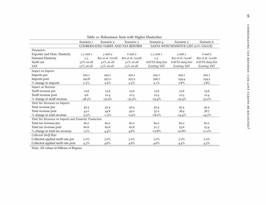
56

co

or

din

at

in

gt

ax

re

fo

rm

s:c

an

lo

st

ta

rif

fs

be

re

co

up

ed

?

Table 10: Robustness Tests with Higher ElasticitiesScenario 1 Scenario 2 Scenario 3 Scenario 4 Scenario 5 Scenario 6

COORDINATED TARIFF AND TAX REFORM SAFTA WITH SENSITIVE LIST (10% VALUE)ParametersExporter and Dom. Elasticity 1.5 and 1 3 and 2 6 and 2 1.5 and 1 3 and 2 6 and 2Demand Elasticity 0.5 Kee et al. (2008) Kee et al. (2008) 0.5 Kee et al. (2008) Kee et al. (2008)Tariff cut 50% on all 50% on all 50% on all SAFTA duty-free SAFTA duty-free SAFTA duty-freeVAT 13% on all 13% on all 13% on all Existing VAT Existing VAT Existing VAT

Impact on ImportsImports pre 222.1 222.1 222.1 222.1 222.1 222.1Imports post 222.8 227.0 227.2 226.7 239.4 239.5% change in imports 0.3% 2.2% 2.3% 2.1% 7.8% 7.8%Impact on RevenueTariff revenue pre 15.6 15.6 15.6 15.6 15.6 15.6Tariff revenue post 9.6 10.4 10.5 10.4 10.5 10.4% change in tariff revenue -38.3% -32.9% -32.5% -33.4% -32.4% -33.2%Total Tax Revenues on ImportsTotal revenue pre 45.4 45.4 45.4 45.4 45.4 45.4Total revenue post 43.0 44.8 45.0 37.2 38.9 38.7% change in total revenue -5.2% -1.2% -0.9% -18.0% -14.4% -14.7%Total Tax Revenues on Imports and Domestic ProductionTotal tax revenue pre 60.0 60.0 60.0 60.0 60.0 60.0Total tax revenue post 60.6 62.6 62.8 51.7 53.6 53.4% change in total tax revenue 1.0% 4.4% 4.6% -13.8% -10.8% -11.0%Collected Tariff RateCollected applied tariff rate pre 7.0% 7.0% 7.0% 7.0% 7.0% 7.0%Collected applied tariff rate post 4.3% 4.6% 4.6% 4.6% 4.4% 4.3%


1.Ba

dd

it

io

na

lt

ab

le

s5

7

Table 11: Change in Price, Production, Revenue, and ProtectionPRICE DOMESTIC PRODUCTION TARIFF REVENUE PROTECTION

ISIC Description Change Pre Post Pre Post Pre Post

With No Sensitive List359 Transport equipment n.e.c. -19.73% 34,153,000 31,399,433 994,567,806 38,676,005 24.20% 0.90%341 Motor vehicles -12.99% 41,464,000 39,204,213 2,138,244,335 918,667,069 28.30% 12.20%141 Quarrying of stone, sand and clay -12.43% 47,421,000 45,091,897 82,464,005 2,583,235 13.90% 0.40%142 Mining and quarrying n.e.c. -17.51% 339,020,000 323,626,886 184,379,204 113,653 28.00% 0.00%261 Glass and glass products -8.99% 20,586,000 19,774,849 124,328,389 30,655,939 11.50% 2.80%12 Farming of animals -7.53% 18,700,000 18,093,203 397,635 328,896 0.20% 0.10%20 Forestry, logging -6.61% 140,000 135,715 4,321,501 1,612,831 7.30% 2.70%269 Non-metallic mineral products -14.66% 10,995,294,000 10,704,445,219 1,144,878,146 59,877,975 17.90% 0.90%343 Parts and accessories for vehicles -5.52% 30,000,000 29,246,069 53,985,555 24,714,072 7.50% 3.40%222 Printing -5.91% 18,826,000 18,394,321 12,190,961 6,569,016 11.00% 5.90%With Sensitive List142 Mining and quarrying n.e.c. -17.51% 339020000 323626886 184379204 113653 28.00% 0.00%261 Glass and glass products -8.26% 20586000 19841379 124328389 40587944 11.50% 3.80%12 Farming of animals -7.53% 18700000 18093203 397635 328896 0.20% 0.10%20 Forestry -6.61% 140000 135715 4321501 1612831 7.30% 2.70%291 General purpose machinery -3.80% 176639000 173603095 191972406 116474391 6.20% 3.70%342 Vehicle bodies, trailers -5.91% 13745000 13516473 2320123 1380290 12.00% 7.20%315 Electric lamps and lighting equipment -3.17% 41907000 41314225 51980453 43377661 9.80% 8.20%271 Basic iron and steel -3.63% 6414842000 6325053323 957951571 287136311 3.80% 1.10%312 Electricity distribution apparatus -2.92% 11228000 11072071 29201055 12864631 3.50% 1.60%289 Fabricated metal products -5.21% 1496438000 1475960021 154013435 79458131 8.60% 4.40%

Note: Top 10 sectors sorted by change in domestic production; values in Rupees


Table 14: Statutory and Applied Tariff RatesStatutory Rate (%) Mean Tariff (%) St. Dev. 25th pct 75th pct Total Obs.

5 4.92 1.37 5 5 53285

10 9.92 0.97 10 10 28254

15 14.88 1.31 15 15 49208

20 19.98 0.56 20 20 26221

30 29.47 3.68 30 30 3320

40 39.68 3.56 40 40 948

80 77.72 13.33 80 80 771

Source: Unpublished data from the Department of Customs, Nepal

Table 12: Major Exporters to Nepal, 2008 & 2010

Partners 2010 (UN COMTRADE) Partners 2008 (Nepal Customs)Economy Value (US$m) Economy Value (US$m)

India 2900.0 India 2064.2China 536.4 China 365.9United Arab Emirates 456.8 Indonesia 104.8Indonesia 110.7 Japan 76.6Thailand 102.6 Singapore 76.5United Kingdom 99.8 Thailand 64.7Japan 85.7 Malaysia 56.7Korea, Rep. 80.5 Argentina 51.0United States 73.7 United States 46.4Argentina 68.9 Germany 34.9Singapore 68.5 Saudi Arabia 32.0Australia 67.7 Korea, Rep. 30.7Hong Kong, China 57.8 Taiwan, China 22.3Malaysia 57.5 United Arab Emirates 21.5Switzerland 37.5 United Kingdom 21.5

Note: Different sources and years used for check of consistency

Table 13: Number of Products in the Sensitive ListsIn use as of 2010 Agreed reduction In effect from November 2011

Afghanistan 1072 214 858

Bangladesh 1233* 246* 987*1241** 248** 993**

Bhutan 150 0 150

India 480* 96* 384*868** 173** 695**

Maldives 681 136 545

Nepal 1257* 251* 1006*1295** 259** 1036**

Pakistan 1169 233 936

Sri Lanka 1042 208 834

Source: SAARC Secretariat; *For LDCs, ** For Non-LDCs

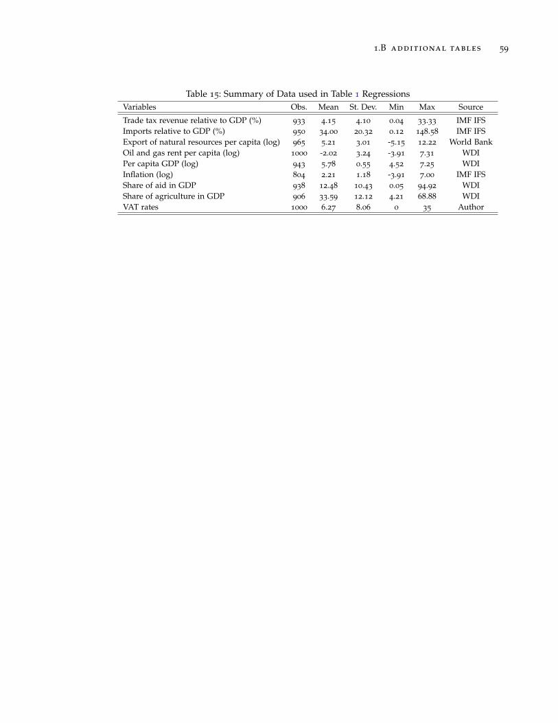
1.B additional tables 59

Table 15: Summary of Data used in Table 1 RegressionsVariables Obs. Mean St. Dev. Min Max Source

Trade tax revenue relative to GDP (%) 933 4.15 4.10 0.04 33.33 IMF IFSImports relative to GDP (%) 950 34.00 20.32 0.12 148.58 IMF IFSExport of natural resources per capita (log) 965 5.21 3.01 -5.15 12.22 World BankOil and gas rent per capita (log) 1000 -2.02 3.24 -3.91 7.31 WDIPer capita GDP (log) 943 5.78 0.55 4.52 7.25 WDIInflation (log) 804 2.21 1.18 -3.91 7.00 IMF IFSShare of aid in GDP 938 12.48 10.43 0.05 94.92 WDIShare of agriculture in GDP 906 33.59 12.12 4.21 68.88 WDIVAT rates 1000 6.27 8.06 0 35 Author


Table 16: List of Countries and Related Tax Data, 2002-2006

Country Total Tax Rev. Domestic Tax Rev. Trade Tax Rev. VAT rate

Bangladesh 9.1 6.6 2.5 15

Benin 14.1 11.9 2.1 18

Bhutan 10.4 10.0 0.4 .Burkina Faso 10.5 9.0 1.5 18

Burundi 17.9 15.0 3.0 .Cameroon 21.1 19.0 2.2 19.3Central African Republic 8.9 7.3 1.6 18

Chad 7.3 5.2 2.1 18

Comoros 10.3 . . .Congo, Rep. 11.5 9.8 1.7 18.9Cote d’Ivoire 15.2 10.2 5.0 18

Ethiopia 13.0 10.5 2.5 .Gambia, The 22.0 . . .Ghana 17.5 13.4 4.1 12.5Guinea 10.9 9.1 1.8 18

Haiti 8.3 6.1 2.2 10

India 8.8 7.0 1.8 .Indonesia 11.6 11.0 0.6 10

Kenya 17.9 16.1 1.8 16

Lesotho 35.6 15.3 20.3 .Madagascar* 9.4 6.2 3.1 18

Malawi 18.4 16.3 2.1 17.5Mali 14.1 . . 15

Mozambique 10.7 8.8 1.9 17

Myanmar* 4.4 3.7 0.8 .Nepal 8.9 6.0 2.9 13

Niger 10.1 5.4 4.7 19

Nigeria 13.1 9.5 3.6 5

Pakistan 11.8 10.3 1.6 15

Papua New Guinea 20.3 18.7 1.6 10

Rwanda 12.1 10.5 1.7 18

Sao Tome and Principe 19.5 14.6 4.9 .Senegal 16.9 13.8 3.1 18

Sierra Leone 12.0 5.8 6.1 .Solomon Islands 15.4 9.3 6.1 .Tanzania 11.7 10.6 1.1 20

Togo 11.5 5.6 5.9 18

Uganda 12.3 11.1 1.2 18

Zambia 17.5 15.3 2.3 17.5Zimbabwe 16.8 15.2 1.6 .

Source: Tax data from Baunsgaard and Keen (2010);VAT rates from Krever (2008), Ernst and Young (2008), and Doing Business indicatorsNote 1: Revenue figures are relative to GDP (in percent)Note 2: Average years for starred countries (*) is 1997-2001

coordinating tax reforms in the poorest...

Documents