cooperative predictive control to enhance power system
TRANSCRIPT

Cooperative Predictive Control
to enhance Power System Security
Zur Erlangung des akademischen Grades eines
Doktor-Ingenieurs
von der Fakultat furElektrotechnik und Informationstechnik
des Karlsruher Institut fur Technologie (KIT)genehmigte
Dissertationvon
Dipl. Ing. Matthias Kahl
aus Recklinghausen
Tag der mundlichen Prufung: 08. Dezember 2014
Hauptreferent: Prof. Dr.-Ing. Thomas Leibfried
Korreferent: Prof. Dr.-Ing. Christian Rehtanz
IEH


Acknowledgements
This thesis has been written during my time at the Institute of Electric Energy Sys-
tems and High-Voltage Technology (IEH) of the Karlsruhe Institute of Technology.
Foremost, I would like to thank my doctoral supervisor Prof. Dr.-Ing. Thomas
Leibfried for the opportunity to write this thesis. Prof. Dr-Ing. Thomas Leibfried
gave me the freedom to explore possible means to enhance Power System Security
and helped me with his insight to keep on track. I am in his debt, since he provided
the needed stability, the trusting relationship and guidance to make this thesis
possible.
My gratitude goes towards my second supervisor Prof. Dr.-Ing. Christian Rehtanz,
who mustered the time to welcome me warmly at his institute, and evaluated the
presented thesis critically.
I would like to thank my colleges of the Institute of Electric Energy Systems and
High-Voltage Technology (IEH) for the great team spirit, the fun we had and for
the creative environment.
My deepest gratitude goes towards my supervised students, without their help and
countless hours they invested this thesis would not have been possible. Especially,
I would like to thank Claudius Freye, Lennart Merkert and Simon Wenig for their
excessive commitment.
Last but not least, I would like to thank Dr. Kym Watson for prove reading the
entire thesis and for supporting me.
V

VI

Contents
1 Introduction . . . . . . . . . . . . . . . . . . . . . 3
1.1 Motivation . . . . . . . . . . . . . . . . . . . . 3
1.1.1 Stationary operation . . . . . . . . . . . . . . 4
1.1.2 Transient operation . . . . . . . . . . . . . . 5
1.2 Contributions . . . . . . . . . . . . . . . . . . . 5
1.3 Thesis Outline . . . . . . . . . . . . . . . . . . 6
1.4 List of Publications . . . . . . . . . . . . . . . . . 7
2 Model predictive control . . . . . . . . . . . . . . . . . 9
2.1 Receding horizon control . . . . . . . . . . . . . . . 10
2.2 Model predictive control without constraints . . . . . . . . 10
2.3 Model predictive control with constraints . . . . . . . . . 12
3 Cooperative Multi-area Optimization . . . . . . . . . . . . 15
3.1 Introduction . . . . . . . . . . . . . . . . . . . 15
3.1.1 Coordination of control areas to ensure operational security . 16
3.1.2 Multi-area optimization . . . . . . . . . . . . . 17
3.2 Power Node Framework . . . . . . . . . . . . . . . 19
3.2.1 Dispatch Formulation . . . . . . . . . . . . . . 19
3.2.2 Redispatch Formulation . . . . . . . . . . . . . 21
3.2.3 Network mapping . . . . . . . . . . . . . . . 22
3.2.4 Modeling example - Dispatch Problem . . . . . . . . 23
3.3 Feasible Cooperation MPC . . . . . . . . . . . . . . 28
3.3.1 Cooperation of control areas . . . . . . . . . . . 28
3.3.2 Cooperative Dispatch . . . . . . . . . . . . . . 30
3.3.3 Cooperative Redispatch . . . . . . . . . . . . . 32
3.3.4 Initial Values. . . . . . . . . . . . . . . . . 34
3.3.5 Complexity . . . . . . . . . . . . . . . . . 34
3.4 Case Study. . . . . . . . . . . . . . . . . . . . 35
3.4.1 General setup . . . . . . . . . . . . . . . . 35
3.4.2 IEEE 14 network . . . . . . . . . . . . . . . 36
3.4.3 IEEE 118 network . . . . . . . . . . . . . . . 40
VII

Contents
3.5 Conclusion . . . . . . . . . . . . . . . . . . . . 41
3.5.1 Outlook . . . . . . . . . . . . . . . . . . 42
4 Dynamic Security . . . . . . . . . . . . . . . . . . . 43
4.1 Motivation . . . . . . . . . . . . . . . . . . . . 43
4.1.1 Network Model Overview and Applications . . . . . . 45
4.2 Dynamic network model . . . . . . . . . . . . . . . 46
4.2.1 State Space Formulation . . . . . . . . . . . . . 48
4.2.2 dq-Transformation of the model . . . . . . . . . . 49
4.3 Model of the Synchronous Generator . . . . . . . . . . . 51
4.3.1 Nonlinear Model . . . . . . . . . . . . . . . 51
4.3.2 Torque equations . . . . . . . . . . . . . . . 54
4.3.3 Reference Frame Theory . . . . . . . . . . . . . 54
4.3.4 Linearized Model . . . . . . . . . . . . . . . 55
4.4 External Loads and Static Var Compensator . . . . . . . . 58
4.4.1 External Loads . . . . . . . . . . . . . . . . 58
4.4.2 Static Var Compensator . . . . . . . . . . . . . 58
4.5 Overall model including dynamic network and generators . . . . 61
4.6 Interaction of Grid, Generators and SVCs . . . . . . . . . 62
4.6.1 Applications small signal stability . . . . . . . . . . 63
4.7 Eigenvalue comparison . . . . . . . . . . . . . . . . 64
4.7.1 Evaluation of the dynamic network model . . . . . . . 65
5 State Estimation . . . . . . . . . . . . . . . . . . . 73
5.1 Observer . . . . . . . . . . . . . . . . . . . . 73
5.2 Results . . . . . . . . . . . . . . . . . . . . . 75
6 FC-MPC to improve dynamic stability . . . . . . . . . . . . 77
6.1 Motivation . . . . . . . . . . . . . . . . . . . . 77
6.1.1 Literature Review . . . . . . . . . . . . . . . 78
6.1.2 Controller Structure . . . . . . . . . . . . . . 79
6.2 Modeling Framework . . . . . . . . . . . . . . . . 81
6.3 Feasible Cooperation MPC . . . . . . . . . . . . . . 82
6.3.1 Model manipulation . . . . . . . . . . . . . . 82
6.3.2 Objective Function . . . . . . . . . . . . . . . 85
6.3.3 Implementation . . . . . . . . . . . . . . . . 86
6.3.4 Simulation Results - 2 Area Network . . . . . . . . . 87
6.3.5 Simulation Results - 5 Area Network . . . . . . . . . 89
6.3.6 Discussion. . . . . . . . . . . . . . . . . . 94
6.3.7 Conclusion . . . . . . . . . . . . . . . . . 95
VIII

Contents
7 Conclusion and Outlook . . . . . . . . . . . . . . . . . 97
7.1 Outlook . . . . . . . . . . . . . . . . . . . . . 98
A Control Theory . . . . . . . . . . . . . . . . . . . . 101
A.1 Linearization of a nonlinear system around an operating point . . 101
A.2 Discretization of linear state space models . . . . . . . . . 102
B Multiband PSS . . . . . . . . . . . . . . . . . . . . 103
C Network Data . . . . . . . . . . . . . . . . . . . . 105
C.1 SVC Example . . . . . . . . . . . . . . . . . . . 105
C.2 IEEE 14 Network . . . . . . . . . . . . . . . . . 106
C.3 IEEE 118 Network . . . . . . . . . . . . . . . . . 108
C.4 2 Area Network . . . . . . . . . . . . . . . . . . 122
C.5 5 Area Network . . . . . . . . . . . . . . . . . . 123
IX

Contents
X

Kurzfassung
Durch den starken Ausbau erneuerbarer Energiequellen erhoht sich der Anteil von
volatiler Einspeisung immer weiter. Folglich sind zu Zeiten von einem hohem Wind
bzw. Solarenergie aufkommen auch weniger konventionelle Kraftwerke am Netz.
Durch den steigenden Bedarf an Energieubertragung ist die Leitungskapazitat hau-
figer ausgeschopft, sodass eingreifende Maßnahmen notwendig sind. Ziel der Ar-
beit ist es die Versorgungssicherheit bei auch bei stark ausgelasteten Netzen zu
gewahrleisten.
Die Versorgungssicherheit muss zunachst fur den stationaren Betrieb sichergestellt
werden. Hierfur wird uberpruft, ob fur einen geplanten Kraftwerksfahrplan keine
Betriebsmittel uberlastet werden. Dieses Problem wird in der Arbeit als Opti-
mierungsproblem aufgefasst, wobei mehrere Regelzonen unter Berucksichtigung von
Speichern und regenerativer Energieerzeuger optimiert werden sollen.
Der zweite Teil der Arbeit optimiert das Verhalten nach einem Storfall, hierzu
zahlen Kurzschluss, Kraftwerksblockausfall und Leitungsausfall. Um das transiente
Verhalten des Energieubertragungssystems zu verbessern, wird ein Systemmodell
verwendet, welches explizit Regler-Interaktionen berucksichtigt und eine Vielzahl
von Dampfungssystemen koordiniert. Fur die Koordination kommt ein Weitbere-
ichsuberwachungssystem zum Einsatz.
In der Dissertation kommen verteilte kooperative Regelstrukturen zum Einsatz um
der Komplexitat und Große des Energieubertragungssystems Rechnung zu tragen.
Die Arbeit beschaftigt sich mit der Formulierung von kooperativen Gutekriterien,
die eine bessere Performance zu ermoglichen als bei der Verwendung von dezentrale
Verfahren.
1

2

Chapter 1
Introduction
1.1 Motivation
Power systems are under an elementary stress to change. With the rising number
of renewable energy sources (RES) the fundamental methods for power system
planning, operation and security of supply have to be validated and updated as
needed. RES are volatile, leading to several problems. Conventional generation or
storage devices need to close the gap between demand and supply. The network
needs to support high RES feed-in. If that happens rarely, the produced energy does
not justify the costs for network reinforcements. Hence, an economically planned
network does include curtailment of RES. On the other hand, optimal operation is
attained by using curtailment of RES as little as possible. While conventional power
generation was concentrated at well planned connection points, RES are built in
areas where environmental conditions (i.e. high wind potential) are most suitable.
Not only the expansion of RES has increased the strain on the grid significantly,
but also the growing demand for electrical power and the hesitant expansion of the
power grid. Consequently, transfer capacities can reach their limits and corrective
actions are needed more frequently. An optimal operation of a stressed network with
a high share of volatile RES leads to a high number of redispatch events. Further-
more, the transient performance of a stressed network is in particular challenging.
The high number of RES makes the overall behavior difficult to control.
With the unbundling of energy generation, transmission and sales, the transmission
system operator (TSO) has the obligation to guarantee safe operation and should
exploit all possibilities to comply with physical and normative constraints at mini-
mum costs. Safe operation can be divided into safe stationary operation and safe
transient operation.
This thesis presents novel procedures to implement and guarantee safe operation in
both stationary and dynamic situations.
3

1 Introduction
1.1.1 Stationary operation
Stationary operation includes the balance of supply and demand, the compliance
with thermal lines rating, voltage constraints and maximum power output of power
plants. Safe dynamic operation includes the dynamically stable system behavior
influenced by the generators in operation and the operation condition of the network.
As depicted in Fig. 1.1 fulfilled stationary constraints and dynamic stability need
to be guaranteed for a planned schedule. The transmission dispatch system checks
if a planned schedule is within operating constraints and guarantees safe operation.
Based on [68] a high level functional representation of a transmission dispatch sys-
tem is shown in Fig. 1.1. This thesis treats the dispatch and the dynamic opera-
tional security modules. The transmission dispatch system is based on the network
Model Predictive Dispatch
Voltage Security
Assessment
Dynamic Security
Assessment
Updated Operating Constraints
Network DataSupply and demand
forecastDispatch Prices
Transmission Dispatch System
Secure & Efficient Dispatch
Secure Secure Secure
Insecure Insecure
Figure 1.1: Block diagram of transmission dispatch system
data, supply/load predictions and dispatch costs. The model predictive dispatch
calculates an optimal trajectory dispatching all available units with minimum costs.
The method as presented in Chapter 3 also includes storage devices and RES feed-
in predictions. The calculated schedule is evaluated with a security constrained
optimal power flow (SC-OPF) ensuring voltage security. If no secure power flow
ensuring voltage constraints exists for the planned schedule, the constraints of the
dispatch function are updated. In case the planned schedule is within the defined
constraints, the schedule is further validated by the dynamic security assessment.
A dynamic model of the system as presented in Chapter 4 is used for the dynamic
security assessment. Analogously to the voltage security assessment, constraints
are adapted, if the proposed operating schedule is dynamically unstable and the
model predictive dispatch will be executed again. In case the operating schedule is
dynamically secure, appropriate set points are communicated to generation opera-
tors.
4

1.2 Contributions
1.1.2 Transient operation
Although dynamic security is verified during stationary operation, methods to ex-
tend the dynamic operating range of power systems are of great importance. They
improve operational flexibility and the security of supply. Modes with poor or even
negative damping, which limit the operating range, are created by weak intercon-
nections. The performance after line outages, short circuits and generator unit
losses is of paramount importance. Outages of long duration cause enormous eco-
nomic losses. The most economic solutions to damp low frequency oscillations are
PSS and dampening strategies for FACTS & HVDC. Alternatives like operating
restrictions or transmission extensions, are very costly compared to active damping
approaches.
Power systems with several generator units, FACTS, HVDC and transformers with
on-load-tap-changer operate with a multitude of control loops which may interact.
Multiple-input and multiple-output (MiMo) system description explicitly accounts
for the interactions mentioned above. Control methods relying on MiMo models
can coordinate all controllable devices effectively and therefore provide dynamic
stability and good transient behavior. Coordination of a large number of devices
requires a systematic control design approach.
1.2 Contributions
• A distributed problem formulation is introduced to integrate RES and storage
devices optimally during stationary operation.
• An advanced model predictive dispatch system is developed within the pre-
sented transmission dispatch system of Fig. 1.1. The algorithm dispatches
conventional generation, RES and storage devices. Load and generation pre-
dictions are considered. Optimal schedules are attained for several control
areas through a cooperative approach.
• A system model is presented that describes control interactions and includes
network dynamics. The advanced model can be used in the transmission
dispatch system to guarantee dynamic security and for controller synthesis
explicitly considering control interaction.
• An eigenvalue comparison is carried out, comparing models relying on static
network equations and models relying on dynamic network equations.
• A dynamic state estimator is developed, using dynamic network equations.
The estimator is able to calculate voltage absolute value and angle of tran-
sients with sparse measurements.
5
1 Introduction
• An integral control strategy is presented which applies data from phase mea-
surement units to damp inter-area oscillations. The proposed distributed
model predictive control method realizes one control unit for each control-
lable device (Generators, FACTS, HVDC), and coordinates their behavior
after a fault. Each unit is designed by applying a systematic controller syn-
thesis.
1.3 Thesis Outline
Chapter 2 gives an overview of model predictive control, which was applied
throughout this thesis as a control and optimization method. This method will
be introduced and explained.
Chapter 3 adapts model predictive control to power systems in stationary oper-
ation. Both dispatch and redispatch formulations are developed. The approach
is further extended to cooperative dispatch and redispatch methods, which can be
applied to an interconnected network, optimizing several control areas. Simulation
results are presented using benchmark networks with 14 and 118 nodes respectively.
Chapter 4 provides a model formulation valid for dynamical processes in power
systems. Models for synchronous generators, Static Var Compensators and the
network are introduced. An eigenvalue comparison of models relying on static
network equations and models relying on dynamic network equations is conducted.
Chapter 5 develops a state estimator, which is able to track absolute value and
angle of voltages during transient events.
Chapter 6 presents a cooperative MPC strategy, which enhances the performance
of PSS using the network state as a global signal. Simulation results are obtained
using 11 and 59 node benchmark networks respectively.
Chapter 7 concludes with a summary of the presented work and an outlook.
6

1.4 List of Publications
1.4 List of Publications
M. Kahl, C. Freye, T. Leibfried: ”A Cooperative Multi-area Optimization with
Renewable Generation and Storage Devices”, IEEE Transactions on Power Systems
2014
M. Kahl, D. Uber, T. Leibfried: ”Dynamic State Estimator for voltage stability
and low frequency oscillation detection”, IEEE Innovative Smart Grid Technologies
Conference- Asia, Malaysia 2014
M. Kahl, S. Wenig, T. Leibfried: ”Dezentrale modellpradiktive Optimierungsstrate-
gien zur Einbindung erneuerbarer Erzeugungskapazitat und Speichersysteme”, Kon-
ferenz fur Nachhaltige Energieversorgung und Integration von Speichern-NEIS, Ham-
burg 2013
M. Kahl, T. Leibfried: ”Decentralized Model Predictive Control of Electrical Power
Systems”, International Conference on Power Systems Transients (IPST2013) in
Vancouver, Canada 2013
M. Kahl, T. Leibfried: ”Stabilitatsanalyse von stromrichterbetriebenen Anlagen zur
Blindleistungskompensation und deren Auslegung”, VDE Kongress, Stuttgart 2012
M. Kahl, T. Leibfried: ”Modellbasierte Regelungsalgorithmen fur das Energienetz
der Zukunft”, IT fur die Energiesysteme der Zukunft, Lecture Notes in Informatics
(LNI), Berlin 2011
U. Reiner, M. Kahl, T. Leibfried, F. Allerding, H. Schmeck: ”MeRegioMobil-Labor -
Entwicklungsumgebung fur zukunftige Smart-homes”, ETG Kongress, Leipzig 2010
7

8

Chapter 2
Model predictive control
The used methodology for all security enhancing measures presented in this thesis
originates from model predictive control. Model predictive control (MPC) is a
control method, which relies on a dynamic model [57]. With the developed model
the predicted behavior of the plant is optimized applying an objective function. As
depicted in Fig. 2.1 the controller considers predicted plant behavior. The optimal
trajectories for all control variables are calculated over a horizon. Furthermore,
MPC can explicitly account for constraints like a maximal rate of change or a
control variable limit. Hence, an operation close to the operational limits is possible,
which increases overall productivity.
MPC is a multiple input multiple output (MiMo) control method, which is able
to implement a controller for several control variables and can incorporate several
measurement systems, while explicitly account for system coupling.
The number of control variables and measurement variables can be adapted on-
line without the necessity of controller reconfiguration. Each power plant can be
integrated, seamlessly if it joins or drops out of interconnected operation.
Prediction
Control var.
Optimization horizon N
t
Figure 2.1: Observer structure
9

2 Model predictive control
2.1 Receding horizon control
Receding horizon control describes the working principle of MPC. MPC is based
on a process model, which is used to predict the behavior of the plant. The opti-
mization horizon is the time interval for which the prediction is executed and the
influence of the control variables are considered. The optimization horizon has the
length N . The optimization takes place over the entire optimization horizon; how-
ever only the first steps of the calculated control sequence is applied. The length of
the applied control sequence is called optimization frequency. The control method
looks continually ahead to optimize current and future decisions, to achieve better
performance compared to one step methods without prediction. Depending on the
agility of the underling process the length of the optimization horizon needs to be
adapted. Slow evolving chemical systems or quasi-static power systems as in Chap-
ter 3 have for example long prediction horizons, whereas fast evolving transients as
discussed in Chapter 6 may only have an optimization horizon of a few steps.
One way to ease the computable burden is to increase the length of the applied
control sequence (i.e. optimization frequency). However, due to model and mea-
surement errors the performance of the controller may suffer significantly. In this
thesis MPC is used as a superordinate system and will only calculate new set points
for fast acting PI-controllers. This fact decreases the vulnerability to communica-
tion delays.
2.2 Model predictive control without constraints
In order to compute a model predictive controller, a forecast for the state variable
x(1) ... x(N) is needed. The variable is calculated with the help of the current state
variable x(0) and a potential input sequence u(0) ... u(N).
Power systems can be described with a discrete state space system of the form
x(k + 1) = Ax(k) +Bu(k), (2.1)
where x is the state vector, u is the vector of control variables, A is the time discrete
system matrix and B is the time discrete input matrix. With the help of (2.1) the
prediction is realized. Moreover, (2.1) is equal to the first prediction step.
The second step with k ⇒ k + 1 is
x(k + 2) = Ax(k + 1) + Bu(k + 1)
= A2x(k) + ABu(k) + Bu(k + 1).(2.2)
10

2.2 Model predictive control without constraints
Consequently, the equation for the N -th prediction step is
x(k +N) = ANx(k) + A(N−1)Bu(k) + . . . + Bu(k +N − 1). (2.3)
The optimal trajectory u∗ = [u(0), u(1), . . . , u(N − 1)]∗ is calculated with the help
of a positive definite objective function φ over the optimization horizon N . A
quadratic cost function, which optimizes both control and state variables is defined
with
minu
φ(u, x(0)) =
N∑k=1
uT (k − 1)Ru(k − 1) + x(k)TQx(k), (2.4)
where R and Q are positive definite weighing matrices. With (2.1 - 2.3) and k = 0, a
prediction of state variables in dependence of the current and future control variable
inputs as well as the initial values x(0) is given through
x(1)
...
...
x(N)
︸ ︷︷ ︸
x
=
A......
AN
︸ ︷︷ ︸
Sx
x(0) +
B 0 . . . 0
AB. . .
. . ....
.... . .
. . ....
AN−1B . . . . . . B
︸ ︷︷ ︸
Su
u(0)
u(1)...
u(N − 1)
︸ ︷︷ ︸
u
.
(2.5)
The weighing matrices may change over the course of the optimization horizon and
can also be expressed in block diagonal matrix form
Q =
Q(1) 0
. . .
0 Q(N)
, R =
R(0) 0
. . .
0 R(N − 1)
. (2.6)
The objective function (2.4) formulated in matrix form is
φ(u, x(0)) = xT Qx+ uT Ru. (2.7)
The state vector x is replaced in (2.7) with (2.5). Hence the objective function is
given through
φ(u;x(0)) = uT (STu QSu + R)︸ ︷︷ ︸H
u+ 2xT (0) (STx QSu)︸ ︷︷ ︸F
u+ xT (0) (STx QSx)︸ ︷︷ ︸Y
x(0)
= uTHu+ 2x(0)TFu+ xT (0)Y x(0).
(2.8)
11
2 Model predictive control
Since the positive definiteness of R is transferable to H (2.8) is a positive definite
QP-problem. Hence, the minimum of (2.8) is calculated with
∂φ(u;x(0))
∂u= 0 (2.9)
and the optimal trajectory is given through
u∗(x(0)) = −H−1FTx(0). (2.10)
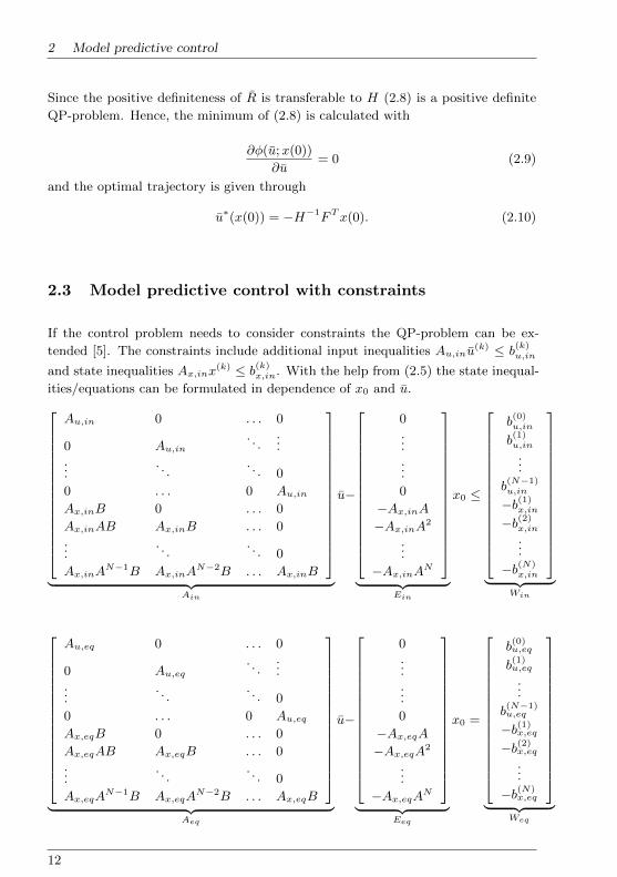
2.3 Model predictive control with constraints
If the control problem needs to consider constraints the QP-problem can be ex-
tended [5]. The constraints include additional input inequalities Au,inu(k) ≤ b
(k)u,in
and state inequalities Ax,inx(k) ≤ b(k)
x,in. With the help from (2.5) the state inequal-
ities/equations can be formulated in dependence of x0 and u.
Au,in 0 . . . 0
0 Au,in. . .
......
. . .. . . 0
0 . . . 0 Au,inAx,inB 0 . . . 0
Ax,inAB Ax,inB . . . 0...
. . .. . . 0
Ax,inAN−1B Ax,inA
N−2B . . . Ax,inB
︸ ︷︷ ︸
Ain
u−
0......
0
−Ax,inA−Ax,inA2
...
−Ax,inAN
︸ ︷︷ ︸
Ein
x0 ≤
b(0)u,in
b(1)u,in
...
b(N−1)u,in
−b(1)x,in
−b(2)x,in
...
−b(N)x,in
︸ ︷︷ ︸
Win
Au,eq 0 . . . 0
0 Au,eq. . .
......
. . .. . . 0
0 . . . 0 Au,eqAx,eqB 0 . . . 0
Ax,eqAB Ax,eqB . . . 0...
. . .. . . 0
Ax,eqAN−1B Ax,eqA
N−2B . . . Ax,eqB
︸ ︷︷ ︸
Aeq
u−
0......
0
−Ax,eqA−Ax,eqA2
...
−Ax,eqAN
︸ ︷︷ ︸
Eeq
x0 =
b(0)u,eq
b(1)u,eq
...
b(N−1)u,eq
−b(1)x,eq
−b(2)x,eq
...
−b(N)x,eq
︸ ︷︷ ︸
Weq
12

2.3 Model predictive control with constraints
minu
φ(u, x0) = uTHu+ 2xT0 Fu+ x0TY x0 (2.11)
The objective function (2.4) in the general form is extended with equalities and
inequalities constraints
Ainu ≤Win + Einx0︸ ︷︷ ︸bin
(2.12)
Aequ = Weq + Eeqx0︸ ︷︷ ︸beq
. (2.13)
As promising and potent as MPC might be, power systems pose a very complex
system and therefore optimization problem. MPC in large scale applications is
under research, but practical implementations in the industry are limited.
Partitioning a large scale problem into sub-systems, can effectively reduce the com-
putational complexity. In Chapter 3 and Chapter 6 cooperative measures are intro-
duced, which will compute a solution close to the global optimum and reduce the
computational complexity.
13

14

Chapter 3
Cooperative Multi-area Optimization
3.1 Introduction
In Chapter 1.1.1 an overview is given on how secure stationary operation is guar-
anteed. This approach increases flexible grid operation and allows TSOs to reduce
redispatch costs caused by intermittent renewable energy sources (RES). The coop-
erative multi-area optimization strategy presented here enables transmission system
operators (TSOs) to dispatch/redispatch interconnected networks securely, while re-
ducing dispatch/redispatch costs. Schedules for storage devices, conventional- and
renewable generation are obtained considering network constraints and ramping
rates [80]. An optimal schedule for several control areas is attained, including
storage operation to achieve congestion relief. The distributed approach preserves
control area responsibilities. All participating control areas attain a schedule close
to the global optimum. TSOs implement agreements to share resulting profits.
Problem decomposition reduces the complexity compared to a global optimization
and makes it suitable for large scale optimization. The multi-step optimization
considers RES and load forecast over an optimization horizon. The functionality
was shown successfully using stressed 14 and 118 node systems. A cross border
dispatch with use of storage devices is realized to maintain a high share of RES
feed-in, while reducing overall dispatch costs.
In an unbundled market environment each market player receives unrestricted ac-
cess to the market and therefore to the network. The TSO validates the day-ahead
schedule for adherence to standards for a secure operation of the transmission sys-
tem. Several arrangements are in place to avoid day-ahead congestion and make
efficient operation possible. However, in case temporary or unexpected congestion
arises, the TSO is obliged to alter the power flow with all necessary means. Possible
means are topology changes, the use of FACTS elements, redispatch of generation
and RES curtailment. This chapter focuses on the efficient short term dispatch and
redispatch of generation, RES curtailment and storage operation.
15

3 Cooperative Multi-area Optimization
Redispatch volume and costs are becoming increasingly significant factors in grid
operation. The main drivers of this trend are: the hesitant extensions of the power
grid, the expansion of RES and the growing demand for electrical power. Further-
more, the introduction of energy trading through a common market has led to
an additional aggravation of the problem. In Europe generator unit locations are
selected solely by economical considerations, whereas costs of transmission grid rein-
forcements are not considered. The increasing redispatch and control power costs in
Europe can be avoided partially by using a shorter dispatch interval. With the ap-
plied dispatch interval of up to 1 hour, TSOs need to operate the power system well
within its physical limits [19]; for comparison Australia is using a 5 minute dispatch
interval. As a second measure to reduce redispatch cost and volume, cooperative
redispatch strategies involving several control areas are promising.
Network operational flexibility is essential to accommodate a high share of RES.
Means to enable more flexibility are storage devices, demand side management,
energy balancing from RES and combined heat power plants (CHP), improved
demand and RES feed-in predictions [70]. Furthermore, the ramping capability of
generators has to be taken into account. A lack of coordination between control
areas during dispatch or redispatch may result in non-optimal use of generation or
balancing power [2]. Due to the high costs for storage and hot standby operation
of conventional power plants, grid operation needs to be as close as possible to the
global optimum.
The following chapter presents an advanced dispatch/redispatch algorithm, which
coordinates several control areas optimally including the existing storage devices
and avoids unwanted interaction. Each control area executes a local optimization
with simplified external generation costs. Through iterative calculation of the local
optimization problems, the algorithm converges close to the global optimum.
3.1.1 Coordination of control areas to ensure operational security
In order to guarantee operational security between control areas, the European Net-
work of Transmission System Operators for Electricity (Entso-E) published guide-
lines in the operation handbook [14].
3.1.1.1 N-1 operation
The TSOs are obliged to guarantee operational security within their control zone,
and have the means to redispatch the available generation. The operational security
limits need to hold before and after a contingency took place. Contingencies are
for example line, generator, power station or transformer outages. Operational
security subsumes the N-1 principle, line constraints and generation constraints.
16

3.1 Introduction
The TSO creates a list of possible faults, according to a risk assessment analysis.
External contingencies are possible faults from neighboring control areas. Each
element in the contingency list needs to be considered in the N-1 simulation. An
external contingency is considered in the N-1 simulation, and added to the list, if
there is a considerable influence on its own area. An optimal redispatch restores
the system from a state with possible constraint violations to a system without
constraint violations at minimum redispatch costs.
3.1.1.2 Observability
An online model is implemented to evaluate the network condition and assess the
security situation. The scope of the online model is the observability area including
the own and parts of the neighboring network. The observability area includes all
external contingencies. Each TSO needs to be able to perform N-1 calculations for
any external contingency.
3.1.1.3 Coordination
The Entso-E operation handbook [14] defines the following procedures regarding
TSO interaction:
Collaboration of TSOs is essential and includes the exchange of relevant information
on risks and the preparation of coordinated remedial actions one day in advance as
necessary. Control areas cannot act independently and redispatch strategies often
influence neighboring TSOs. Consequently, a globally optimal redispatch involves
cooperation of TSOs. Desired effects are inter-TSO assistance in the event of fail-
ures and the prevention of disturbances. Communication between neighbors to
change the generation pattern abroad and defined mechanisms to launch cross bor-
der redispatching need to be implemented. The TSOs are able to share information
on redispatching costs with each other.
The above statements, especially those on the cooperation of TSOs, concern redis-
patch and are applicable to short term dispatch as well.
3.1.2 Multi-area optimization
Within the environment defined by the Entso-E a distributed cooperative multi-area
optimization is introduced, with the goal of a cost optimal (re-)dispatch involving
several areas with compliance of constraints.
The advantages are
• defined and controlled way of cross border (re-)dispatching
17

3 Cooperative Multi-area Optimization
• consideration of control area interaction
• more flexible and efficient grid operation
• reduction of (re-)dispatch cost in comparison to a decentralized approach
• consideration of a continuously updated wind forecast
• optimal storage operation to achieve congestion relief
Each TSO conducts its own optimization with inclusion of approximated neighbor-
ing generation costs. The generation pattern, load and RES feed-in forecasts are
exchanged. Through an iterative approach, a solution close to the global optimum
is reached.
As described above and in compliance with [14], the following features are used. The
TSOs exchange the (re-)dispatch costs and prepare a comprehensive network model,
including all participating control areas. Furthermore, TSOs exchange load and
RES feed-in forecasts, current network states and generation patterns. Each TSO
keeps its field of responsibility and independence. Thus, the TSO (re-)dispatches
the generation in its area of responsibility and is able to define individual cost
functions and constraints.
3.1.2.1 Literature Overview
Efficient network operation can be interpreted as an optimization problem under
consideration of constraints. The solution of the optimal power flow (OPF) leads
to an optimized grid operation. Several solution strategies have recently made it
possible to cope with these economic challenges in optimal grid operation. In order
to include storage devices, [13] presented a sequential OPF. The sequential OPF
only considers storage operation over a limited time interval, to ease computational
complexity. In case the full optimization horizon is considered, MPC and sequential
OPF pose the same problem formulation. Several distributed OPF formulations
are available [4], [43]. [39] presented a multi-step optimization and extended the
formulation to a distributed approach with a Lagrangian decomposition [2]. An
extensive review of congestion management is given in [48]. Redispatch strategies
are the focus of [58] and [78]. For example [58] proposes an approach to improve
cross border redispatch. [60] and [51] deploy a generalized Nash equilibrium to
achieve joint cross border redispatch. [6] compares national and joint cross border
redispatch. [78] adapts an OPF formulation to redispatch generation and operate
FACTS devices.
18

3.2 Power Node Framework
3.2 Power Node Framework
This unified modeling framework is able to represent complex structures within
a model environment introduced by [30], [71] and [16]. It can be used to explic-
itly consider renewable energy sources and storage devices. Also energy efficiency,
environmental impact and cost of a technologically diverse unit portfolio can be
evaluated. A model of a power system with consideration of grid and generation
constraints allows optimal operation with the use of a system model. The power
node domain is linked with the grid side under the use of power generation ug and
power demand ul. A power node is described by the following variables. The de-
manded power is denoted by ξ < 0 and the provided power is denoted by ξ > 0.
In case of RES curtailment or unserved load process variables w > 0 or w < 0 are
introduced. A power node is defined in the most general case with
x(k + 1) = Ax(k) + TC−1(ηlul − η−1g ug + ξ − w), (3.1)
where x represents the state of the storage, A is the system matrix and C denotes
the capacity of the storage device. Equation (3.1) is a discrete state space system,
where k is the time variable and T the sample rate. The following model descriptions
were used for the problem formulation.
3.2.1 Dispatch Formulation
3.2.1.1 Generation
The power output of conventional generation such as thermal power plants and
CHP can be chosen arbitrarily. Thus, ug is an optimization variable. ξ represents
the fuel consumption of the plant.
0 = −η−1g (ug) + ξ (3.2)
Constraints include min/max power output and ramping rates.
uming ≤ ug ≤ umaxg
rming ≤ ug(k)− ug(k − 1) ≤ rmaxg
(3.3)
Renewable Energy Sources are curtailable, hence w is an optimization variable. The
process variable ξ is in this case the estimated solar radiation or wind powering the
generator, based on weather forecasts.
0 = −η−1g ug − w + ξ (3.4)
19

3 Cooperative Multi-area Optimization
Since curtailment can never be greater than the estimation of the supply,
0 ≤ w ≤ |ξ|. (3.5)
3.2.1.2 Storage Devices
For each storage device a dynamic equation is introduced
x(k + 1) = x(k) + TC−1(ηlus − η−1g ug), (3.6)
where us denotes storage charging and C denotes the capacity of the storage device.
A state variable change will occur if an imbalance between supply and demand
arises at the power node. Optimization variables are ug and us. The normalized
state variable is limited to a minimum and maximum of stored energy. Constraints
also include min/max power output and ramping rates.
0 ≤ x ≤ 1
uming ≤ ug ≤ umaxg
umins ≤ us ≤ umaxs
(3.7)
rming ≤ ug(k)− ug(k − 1) ≤ rmaxg (3.8)
In order to distinguish between controllable and uncontrollable loads us is intro-
duced as a controllable variable in addition to ul, which is an uncontrollable vari-
able.
3.2.1.3 System formulation
For each power node a corresponding equation of the type (3.1) is deployed. Nodes
with storage can be formulated with
x(k + 1) = Ax(k) + B
(u
z
)(3.9)
and nodes without storage with
0 = B
(u
z
), (3.10)
20

3.2 Power Node Framework
where u is the set of all optimization variables, z is the set of all uncontrollable
variables and A is an identity matrix. (3.9) and (3.10) are time discrete state space
equations, with
B =TC−1(Bg Bs Bw Bξ Bl
)z =
(ξ ul
)Tu =
(ug us w
)T.
(3.11)
3.2.2 Redispatch Formulation
In order to formulate an optimization problem regarding redispatch costs, the dis-
patch formulation of [30] stated in Section 3.2.1 is extended:
ug = ∆ug+ + ∆ug− + ug0 (3.12)
us = ∆us+ + ∆us− + us0 (3.13)
is introduced where ug0/us0 is power generation/demand of the day-ahead schedule.
∆ug+ is the increment of generation and ∆ug− is the decrement of generation.
Furthermore, ∆us+ denotes the increment of charging power, whereas ∆us− denotes
the decrement of charging power. Distinguishing increment and decrement enables
the differentiation of increment and decrement generation costs and avoids nonlinear
equation sets [6].
3.2.2.1 Generation
As a consequence ug is replaced by (3.12) to deduce a redispatch formulation. Hence,
0 = −η−1g (∆ug+ + ∆ug− + ug0) + ξ. (3.14)
Constraints include min/max power output and ramping rates.
0 ≤ ∆ug+ ≤ umaxg − ug0uming − ug0 ≤ ∆ug− ≤ 0
rming ≤ ug(k)− ug(k − 1) ≤ rmaxg
(3.15)
Note for algebraic sign handling, the constraint on ∆ug− ensures ∆ug− ≤ 0.
21

3 Cooperative Multi-area Optimization
3.2.2.2 Storage Devices
Furthermore, ug and us is replaced by (3.12) and (3.13) for storage devices.
x(k + 1) = x(k) + TC−1(ηl(∆us+ + ∆us− + us0)−η−1g (∆ug+ + ∆ug− + ug0))
(3.16)
Analogous to (3.15) the constraints for storage devices are
0 ≤ x ≤ 1
0 ≤ ∆ug+ ≤ umaxg − ug0uming − ug0 ≤ ∆ug− ≤ 0
(3.17)
0 ≤ ∆us+ ≤ umaxs − us0umins − us0 ≤ ∆us− ≤ 0
(3.18)
rming ≤ ug(k)− ug(k − 1) ≤ rmaxg (3.19)
3.2.3 Network mapping
A problem formulation in accordance with the power node framework can be used
with any kind of network model. Possible candidates are DC power model, AC
power model and successive linearization of the AC power model [17], [77], [1].
The power flow model for the case study is a DC power flow. The power flow is
calculated with the admittance matrix BDC .
Pbus = BDC θ (3.20)
The network model can be mapped to the system (3.9), (3.10) with
Pbus =
cT1 bT1cT2 bT2...
...
cTn bTn
︸ ︷︷ ︸
Gmap
(ugul
)(3.21)
where Gmap is a bus mapping matrix and cik and bik are defined with
cik =
0 : no grid injection
1 : generator injectionbik =
0 : no grid injection
−1 : load injection.
22

3.2 Power Node Framework
The bus mapping matrix and admittance matrix are integrated into one equation
set
Gmap
(ugul
)−BDC θ = 0. (3.22)
The transferred power over a line is calculated with
pline −Bfθ = 0 (3.23)
where Bf is the admittance of the corresponding line. (3.22) and (3.23) can also be
replaced by the power transfer distribution factor. pline is limited to the maximum
transfer capacity pmaxline , hence
|pline| − pmaxline ≤ 0. (3.24)
3.2.4 Modeling example - Dispatch Problem
~
Storage
Generator
Load
1 3
2
Figure 3.1: Three node modeling example
The example describes a three node network with one storage device. A combined
heat power plant (CHP) is connected at node 1 and a load is positioned at node 2.
CHP and storage have the following data.
Table 3.1: Generation parameter of a three node example
Pmax in MW Cap. in MW/h ηg ηl Costs in e
CHP 100 0 0.42 / 145Storage 40 5000 0.9 0.85 5
Two lines, with parameters as in Table 3.2, link the corresponding nodes. Opti-
mization variables are ug1, ug2 and us. For the sake of simplicity ramping and line
constraints are neglected. Furthermore, the optimization horizon is N = 1.
23

3 Cooperative Multi-area Optimization
Table 3.2: Line parameter of a three node example
XL in Ω
line 1-2 8line 2-3 2
3.2.4.1 Combined Heat and Power Plant
The power of the CHP is described with (3.25) based on the energy conservation
law. The fuel consumption ξ is the product of efficiency η and the power feed-in.
ξ = η−1g ug1
= 0.42−1ug1(3.25)
Additional constraints for the CHP are
0 ≤ ug1 ≤ 100. (3.26)
3.2.4.2 Storage
The system equation of the storage device can be formulated according to (3.6)
with sample rate T = 15 min = 0.25 h.
x(k + 1) = x(k) + TC−1(−η−1
g ηs)( ug
ul
)
= x(k) +0.25
5000
(−0.9−1 0.85
)( ug2us
) (3.27)
Maximum and minimum constraints are considered with
0 ≤ x ≤ 1
0 ≤ ug2 ≤ 40
0 ≤ us ≤ 40.
(3.28)
The optimization starts with an initial charge of for example 0% (i.e. x(0) = 0).
24
3.2 Power Node Framework
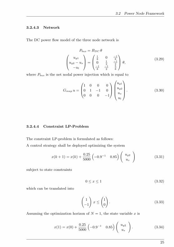
3.2.4.3 Network
The DC power flow model of the three node network is
Pbus = BDC θ ug1ug2 − us−ul
=
18
0 −18
0 12
−12
−18
−12
58
θ,(3.29)
where Pbus is the net nodal power injection which is equal to
Gmap u =
1 0 0 0
0 1 −1 0
0 0 0 −1
ug1ug2usul
. (3.30)
3.2.4.4 Constraint LP-Problem
The constraint LP-problem is formulated as follows:
A control strategy shall be deployed optimizing the system
x(k + 1) = x(k) +0.25
5000
(−0.9−1 0.85
)( ug2us
)(3.31)
subject to state constraints
0 ≤ x ≤ 1 (3.32)
which can be translated into
(1
−1
)x ≤
(1
0
). (3.33)
Assuming the optimization horizon of N = 1, the state variable x is
x(1) = x(0) +0.25
5000
(−0.9−1 0.85
)( ug2us
). (3.34)
25

3 Cooperative Multi-area Optimization
x is replaced in (3.33) with (3.34), which leads to
0.25
5000
(−0.9−1 0.85
0.9−1 −0.85
)(ug2us
)+
(1
−1
)x0 ≤
(1
0
). (3.35)
Let uel =(ug1 ug2 us
)T. In accordance with Chapter 2.3 are the inequalities
formulated with
0.25
5000
(0 −0.9−1 0.85
0 0.9−1 −0.85
) ug1ug2us
≤ (−1
1
)x0 +
(1
0
)
Ain1 uel ≤ bin1.
(3.36)
The input constraints are
0 ≤ug1 ≤ 100
0 ≤ug2 ≤ 40
0 ≤us ≤ 40,
(3.37)
analogous to (3.33) the input constraints are equal to
1 0 0
0 1 0
0 0 1
−1 0 0
0 −1 0
0 0 −1
ug1ug2us
≤
40
100
40
0
0
0
Ain2 uel ≤ bin2.
(3.38)
Additional equations are DC power flow equations (3.29) with
(−Gmap BDC
)︸ ︷︷ ︸
Aeq
uelulθ
= 0. (3.39)
In order to calculate the optimization variables over the course of the optimization
horizon, the demand of the ul is defined by a H0 profile. An equation set for each
time step is defined by the length of the optimization horizon N . The optimization
26

3.2 Power Node Framework
variables ug1 , ug2, us are calculated minimizing the objective function over the
optimization horizon. Consideration of generation costs leads to
φ =
N∑k=1
Lu(k)
=
N∑k=1
145 0 0
0 5 0
0 0 0
ug1(k)
ug2(k)
us(k)
︸ ︷︷ ︸
uel
N=1= Luel
(3.40)
3.2.4.5 Linear Programming
The optimization problem as stated in Section 3.2.4.4 can be solved using the sim-
plex algorithm, which is using an augmented matrix form. The matrix form will
be derived in the following. The inequality constraints are converted into equality
constraints with the introduction of slack variables z. The equation set with slack
variables isφ − Luel = 0
Ainuel + z = bin
Aeq1uel +Aeq2
(ulθ
)︸ ︷︷ ︸uad
= beq,(3.41)
and the corresponding augmented matrix form with the objective to minimize φ is
E −L 0 0
0 Ain 0 E
0 Aeq1 Aeq2 0
φ
ueluadz
=
0
binbeq
with z > 0, (3.42)
where E is an identity matrix. The optimum can be attained by using the simplex
algorithm.
The example has only one dynamic equation, but has 8 inequality constraints and
4 equality constraints. In general, the number of dynamic equations is equal to
the number of storage devices, which is very low compared to the number of con-
straints. Hence, the optimization is primarily static in nature. Cooperation as
introduced by [73], which relies on a coupled system matrix (coupling the state
variables x) will fail, since the matrix is only sparsely populated. In the following
27

3 Cooperative Multi-area Optimization
section novel cooperative optimization strategies have been developed to overcome
these limitations.
3.3 Feasible Cooperation MPC
Goal of the multi-step optimization is to attain the optimal control sequence u∗
over an optimization horizon N , complying with the constraints (3.3), (3.5), (3.7),
(3.8) and (3.24). Predicted RES feed-in and load forecast over the optimization
horizon are considered. Optimization variables are electrical power ug of conven-
tional generation, curtailment w of RES and demand and supply ug, us of storage
devices.
Based on a process model and past control variable inputs u(k − 1), the controller
calculates how changes of the control variables effect the process. The best control
sequence is selected using an objective function. Only the first step of the calculated
control sequence is applied. Subsequently, based on the principle of the receding
horizon, the next step of the optimal control sequence is calculated to account for
prediction and model errors.
3.3.1 Cooperation of control areas
Ensuring a feasible cooperation of control areas, the following requirements have to
be met:
• Through iterative calculation of the local optimization problems, the algo-
rithm shall converge close to the global optimum.
• Communication of the current state and input variables to all subsystems is
mandatory.
• A cooperation is only possible, if a subsystem adapts its state away from its
local optimum towards the global optimum, while demand and supply are
balanced.
• The objective function of each subsystem needs to make a cooperation possi-
ble [73], therefore simplified external generation costs are included.
• Calculated state and input trajectories must satisfy the model and input
constraints of the global system to ensure feasibility.
• The local optimization needs to have a significantly lower complexity in com-
parison to the global problem in order to achieve calculation time benefits.
28

3.3 Feasible Cooperation MPC
x0
Area A Area B
Opt. Area B
x0
comparecosts
eval(costs)eval(costs)
local Opt.+
ext. Gen
Opt. Area A
local Opt.+
ext. Gen
Figure 3.2: Cooperative optimization
A cooperative MPC algorithm is now presented, which complies with the require-
ments stated above.
The procedure is implemented for each subsystem. For the sake of simplicity Fig.
3.2 depicts only two areas. The algorithm starts with an initial condition calculated
with the approach presented in Section 3.3.4. The initial condition includes values
for all subsystems. At the optimization stage the local optimization considers the
sum of external generation and its costs additionally. The costs of the produced
results are evaluated. Results of all control areas are compared and the cheapest
solution is distributed to all areas. Each area uses the favored solution for the next
iteration.
3.3.1.1 Subsystem building
Each subsystem is defined as an area, where the corresponding operator has the
responsibility of a secure network operation and the means to redispatch the gener-
ation units and storage devices. Subsystem m at iterate p is defined through
xpm(k + 1) = Am xpm(k) + Bm
(upmzm
). (3.43)
29

3 Cooperative Multi-area Optimization
Nodes without storage lead to
0 = Bm
(upmzm
). (3.44)
The vector zm is not an optimization variable and is therefore constant during the
iterative process.
Each subsystem defined through (3.43) and (3.44) has no direct coupling to third
party subsystems, the only exchange takes place through the network equations
(3.22). The solution of external subsystems up−1j with ∀j 6= m is made available
for the p-th iteration to subsystem m.
3.3.2 Cooperative Dispatch
The optimization variables are dispatched electrical power ug of conventional gen-
eration, curtailment w of RES and dispatched demand and supply ug, us of storage
devices.
3.3.2.1 Cooperative optimization of generation
At any time throughout the iterative process, the supply is required to be equal
to the demand to fulfill the power flow equations. One control area needs to be
able to influence the power generation in external control areas to achieve power
exchange from one area to another. In order to establish this, one control area has
the ability to reduce the sum of the overall generation of each external control area.
As generation can only be reduced, line limits and generation constraints will always
hold and do not have to be evaluated explicitly. Reduction of generation is also
coherent with the load flow calculation. The described procedure is implemented
for ∀j 6= m with
upg,j = cjup−1g,j (3.45)
where cj is an optimization variable of the dimension (1× 1). External generation
can be reduced from 100% to 0%, which leads to
0 ≤ cj ≤ 1. (3.46)
30

3.3 Feasible Cooperation MPC
3.3.2.2 Cooperative optimization of storage
Storage management is adapted analogously to the cooperative behavior of gen-
eration. The residual charging power available in the storage can be calculated
with
usR = umaxs − us. (3.47)
The remaining storage load of external systems can be accessed with kj and varied
from 0% to 100%. The adapted storage load for ∀j 6= m is
ups,j = up−1s,j + kju
p−1sR,j , (3.48)
where kj is an optimization variable of dimension (1× 1):
0 ≤ kj ≤ 1 (3.49)
Due to the introduction of kj all storage devices of one area can be equally weighted
and thus activated from an external subsystem. In order to prohibit a charging if
the storage device has reached 100% state of charge (SOC) capacity, us is not
allocatable for this time step. Since power generation from storage devices is in the
set of ug, an allocation is implemented analogously to Section 3.3.2.1.
The complexity is reduced significantly since only two additional optimization vari-
ables are needed per external subsystem.
3.3.2.3 Network equation
The exchange of iteration results takes place through (3.20). The vector ug and ulis assembled from all participating TSOs.
ug =(upg,1 upg,2 . . . upg,m
)Tul =
(ul,1 ul,2 . . . ul,m
)T.
(3.50)
The complete equation set (3.20) is kept intact to maintain the coupling of the
optimization problem.
31

3 Cooperative Multi-area Optimization
3.3.2.4 Cost function
The cost function of the m-th subsystem is defined as
φm(um) =
N∑k=1
[Lmum(k − 1) + rm(k)TQmrm(k)
+
M∑j 6=m
Lgen,j(cjup−1g,j )
],
(3.51)
where N is the optimization horizon. Cost matrix of the m-th system Lm includes
generation and curtailment costs, whereas Qm includes ramping costs. Further-
more, costs from external subsystems are also considered, where Lgen,j are the full
dispatch costs. Note that the power of external subsystems up−1gen,j is constant for
each time step.
3.3.3 Cooperative Redispatch
This section describes the realization of cooperative redispatch. The optimization
variables are redispatched electrical power ∆ug of conventional generation, curtail-
ment w of RES and redispatched demand and supply ∆ug,∆us of storages devices.
3.3.3.1 Cooperative optimization of generation
In order to compute a cooperative redispatch strategy of multiple control areas two
optimization variables cj , vj with the dimensions (1 × 1) are introduced. Both
variables are defined within the range
0 ≤ cj ≤ 1
0 ≤ vj ≤ 1(3.52)
and lead as in Section 3.3.2.1 to a reduction of all conventional generation and
storage devices of neighboring subsystems.
∆upg+,j = cj∆up−1g+,j
∆upg−,j = −ug0 + uming + vj(ug0 + ∆up−1g−,j − uming )
(3.53)
cj is capable of reducing any positive deviation of ug0 originated from previous
iterations. Furthermore, vj reduces all conventional generation and storage devices
in neighboring subsystems within the range 0 ≤ ∆ug− ≤ ug0.
The implementation of cooperative optimization of storage devices is described in
Section 3.3.2.2. Equations (3.47), (3.48) and (3.49) are applied.
32
3.3 Feasible Cooperation MPC
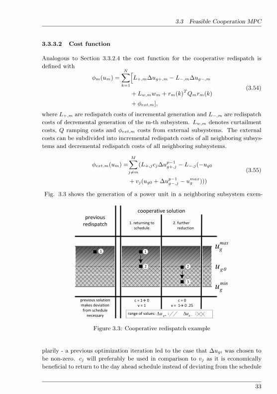
3.3.3.2 Cost function
Analogous to Section 3.3.2.4 the cost function for the cooperative redispatch is
defined with
φm(um) =
N∑k=1
[L+,m∆ug+,m − L−,m∆ug−,m
+ Lw,mwm + rm(k)TQmrm(k)
+ φext,m],
(3.54)
where L+,m are redispatch costs of incremental generation and L−,m are redispatch
costs of decremental generation of the m-th subsystem. Lw,m denotes curtailment
costs, Q ramping costs and φext,m costs from external subsystems. The external
costs can be subdivided into incremental redispatch costs of all neighboring subsys-
tems and decremental redispatch costs of all neighboring subsystems.
φext,m(um) =
M∑j 6=m
(L+,jcj∆up−1g+,j − L−,j(−ug0
+ vj(ug0 + ∆up−1g−,j − umaxg )))
(3.55)
Fig. 3.3 shows the generation of a power unit in a neighboring subsystem exem-
max
gu
min
gu
0gu
g+u gu
Figure 3.3: Cooperative redispatch example
plarily - a previous optimization iteration led to the case that ∆ugi was chosen to
be non-zero. cj will preferably be used in comparison to vj as it is economically
beneficial to return to the day ahead schedule instead of deviating from the schedule
33

3 Cooperative Multi-area Optimization
with vj . Consequently, cj can reduce this neighboring area to ug0 marked in Fig.
3.3 as point 2. If a further power decrease of this unit is profitable, vj is applied
reducing the generated power in this control area within the range ug0 to uming .
This is shown exemplarily in Fig. 3.3 with point 3.
3.3.4 Initial Values
The following algorithm is designed to attain initial values for the cooperative multi-
step optimization.
In phase one a purely decentralized optimization of subsystem m is executed, i.e.
the load and generation of external subsystems are set to zero. System (3.43), (3.44)
is optimized considering the network equations (3.20) with upg,j = 0 and ul,j = 0
∀ j 6= m. A decentralized solution of subsystem m with network constraints is
calculated and communicated to all subsystems. In the second phase a decentral-
ized optimization considering the prior attained solution is executed to produce a
consistent load flow. System (3.43), (3.44) is optimized considering the network
equations (3.20) with up−1g,j and up−1
l,j ∀ j 6= m from the decentralized solution. The
local optimum may not be achieved.x0
Area A Area B
Opt. Area B
x0
comparecosts
eval(costs)eval(costs)
local Opt.+
ext. Gen
Opt. Area A
local Opt.+
ext. Gen
Area A Area B
comparecosts
Decentral Opt.
Opt. Area A
local Opt.
Opt. Area B
local Opt.
Decentral Opt.
Figure 3.4: Flow chart initial values
3.3.5 Complexity
The central dispatch problem formulation has one optimization variable per genera-
tor g including RES and two optimization variables per storage s. Furthermore, two
constraints per generator, four constraints per storage and one constraint per line
34

3.4 Case Study
l are used. Consequently, the number of optimization variables n and the number
of constraints m isn = g + 2s
m = 2g + 4s+ l,(3.56)
Let W = m + n. The complexity can be estimated according to [40] with the big
O notation
O(
(WN)kp). (3.57)
where N is the optimization horizon and kp depends on the solver algorithm used.
The complexity of one subsystem from a total of M subsystems can be estimated
withni = gi + 2si
mi = 2gi + 4si + l,(3.58)
where si and gi denote the number of storage devices and generators in subsystem
i. Let Wi = mi + ni. The complexity per iterate of a subsystem can be estimated
with
O(
((2(M − 1) +Wi)N)kp). (3.59)
Since (2(M − 1) + Wi) W , a significant reduction of complexity is achieved.
Each subsystem can be solved independently using parallel computing methods.
3.4 Case Study
In this section the results of the developed cooperative optimization are presented.
As the central optimization of the considered networks is still solvable, it is possible
to compare the quality of the calculated cooperative optimization. The IEEE 14
and IEEE 118 networks are equipped with additional RES and storage devices.
Simulations are done using Yalmip [55].
3.4.1 General setup
The simulations are conducted with the following assumptions. The process model
has accurate prediction for load and RES feed-in, therefore it possesses perfect
foresight. The N-1 principle is accomplished, if the used line capacity is < 80% of
the rated line capacity. External subsystems cannot dispatch renewable generation
of neighboring systems. Line constraints are defined according to [34]. The scenarios
are defined with a load profile for each load for a period of 72 h. Further, wind
speed and solar radiation are defined for the same time interval.
35

3 Cooperative Multi-area Optimization
3.4.2 IEEE 14 network
The IEEE 14 benchmark network is used to illustrate the capabilities of the devel-
oped algorithm. The case study especially focuses on generation and storage cross
border dispatch. The costs, efficiency η and maximum power output are defined in
Appendix C.2. The generation consists of four biomass power plants, two pumped-
hydro plants, a wind park, a PV and a feeder. The pumped storage plants have a
capacity of 5000 MWh each.
The IEEE 14 network is divided into 4 subsystems as depicted in Fig. 3.5. Both
pumped storage plants are in separate areas. Hence, the subsystems need to coor-
dinate the storage devices and biomass power plants in order to attain an optimal
schedule.
1
42
3
FeederBiomass2
PumpedHydro
Wind1PumpedHydro
Biomass1
Biomass3
Biomass4 Photovoltaics1
LDBUS2
LDBUS3LDBUS4
LDBUS7LDBUS1LDBUS10
LDBUS11
LDBUS12
LDBUS14
LDBUS6
LDBUS13
LDBUS5
Storage2
Storage1
Figure 3.5: Extended IEEE 14 network with RES and storage devices divided intofour areas
3.4.2.1 Cooperative solution
At the beginning of the simulation very high wind feed-in in area 4 endangers grid
security. Area 4 could curtail wind feed-in significantly and solve the incident by
itself. However, from a global perspective it is preferable to use the storage capacity
of area 1. Consequently, both storage devices are charged. Storage 1 is located at
the same busbar as the wind farm and is able to charge with full load (40 MW)
as depicted in Fig. 3.6a. Due to the line restrictions not all wind energy can be
transferred to storage 2. Storage device 2 is able to buffer with a peak load of
36

3.4 Case Study
0 20 40 60
−50
0
50
Time in hours
Pow
erin
MW
Generation Storage 1
Generation Storage 2
Load Storage 1
Load Storage 2
(a) Storage operation
0 20 40 600
50
100
150
200
Time in hours
Pow
erin
MW
Biomass 1
Biomass 2
Biomass 3
Biomass 4
(b) Biomass 1 to 4 operation
0 20 40 600
50
100
150
200
Time in hours
Pow
erin
MW
Curtail.
Wind
Solar
Feeder
(c) Wind power, solar power and feeder operation
Figure 3.6: Cooperative operation of the IEEE 14 network
37
3 Cooperative Multi-area Optimization
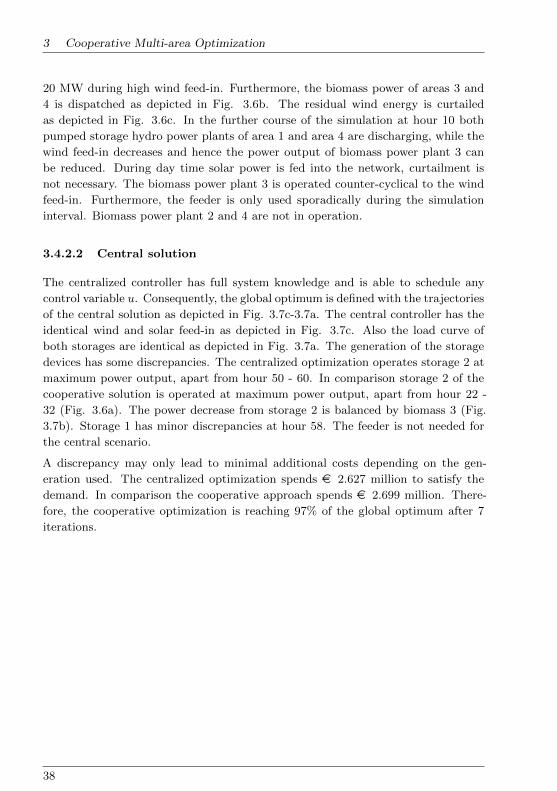
20 MW during high wind feed-in. Furthermore, the biomass power of areas 3 and
4 is dispatched as depicted in Fig. 3.6b. The residual wind energy is curtailed
as depicted in Fig. 3.6c. In the further course of the simulation at hour 10 both
pumped storage hydro power plants of area 1 and area 4 are discharging, while the
wind feed-in decreases and hence the power output of biomass power plant 3 can
be reduced. During day time solar power is fed into the network, curtailment is
not necessary. The biomass power plant 3 is operated counter-cyclical to the wind
feed-in. Furthermore, the feeder is only used sporadically during the simulation
interval. Biomass power plant 2 and 4 are not in operation.
3.4.2.2 Central solution
The centralized controller has full system knowledge and is able to schedule any
control variable u. Consequently, the global optimum is defined with the trajectories
of the central solution as depicted in Fig. 3.7c-3.7a. The central controller has the
identical wind and solar feed-in as depicted in Fig. 3.7c. Also the load curve of
both storages are identical as depicted in Fig. 3.7a. The generation of the storage
devices has some discrepancies. The centralized optimization operates storage 2 at
maximum power output, apart from hour 50 - 60. In comparison storage 2 of the
cooperative solution is operated at maximum power output, apart from hour 22 -
32 (Fig. 3.6a). The power decrease from storage 2 is balanced by biomass 3 (Fig.
3.7b). Storage 1 has minor discrepancies at hour 58. The feeder is not needed for
the central scenario.
A discrepancy may only lead to minimal additional costs depending on the gen-
eration used. The centralized optimization spends e 2.627 million to satisfy the
demand. In comparison the cooperative approach spends e 2.699 million. There-
fore, the cooperative optimization is reaching 97% of the global optimum after 7
iterations.
38

3.4 Case Study
0 20 40 60
−50
0
50
Time in hours
Pow
erin
MW
Generation Storage 1
Generation Storage 2
Load Storage 1
Load Storage 2
(a) Storage operation
0 20 40 600
50
100
150
200
Time in hours
Pow
erin
MW
Biomass 1
Biomass 2
Biomass 3
Biomass 4
(b) Biomass 1 to 4 operation
0 20 40 600
50
100
150
200
Time in hours
Pow
erin
MW
Curtail.
Wind
Solar
Feeder
(c) Wind power, solar power and feeder operation
Figure 3.7: Central operation of the IEEE 14 network
39

3 Cooperative Multi-area Optimization
PV 2
PV 3
21
3
4
5
6
Wind 6
Wind 5
Wind 7
Wind 2Wind 3
Wind 1
Wind 8
Storage 6
Storage 5
Storage 4
Storage 3
Wind 4
Storage 2Storage 1
PV 1
PV 4
PV 7
PV 5
PV 6
1 2
4
5
6 7
8
9
10
11
12
13
14
117
15
16
17
18
19
20
21
22
23
25
26
27
28
29
113 30
31
32
114115
33
34
35
36
37
38
39
40 41 42
43
44
45
4746
48
49
50
51
52
53 54 5556
5758
59
60
61
62
63
64
65
66
67
68
116
69
70
71
72
73
24
74
75
118 76
77
78
79
80
81
82
8384
85
86
87
88 89
9091
92
93
9495
96
97
98
99
100
101102
103
104 105
106
107
108
109
110
111
112
G
G
G
G
G G
G
G
GG
G
G
G
G
G
G
G G
G
G
G
G
G G
G G
G
G G
G
G
G
G
G G G G G
G
G
3
G
G
G
G
G
G
G
G
G
G
G
G
G
G
W
W
W
W
W
W
W
W
P
P
P
P
P
PP S
S
S
SS
S
W
P
S
Wind farm
Photovoltaic
Storage
Figure 3.8: Extended IEEE 118 network with RES and storage devices divided intosix areas
3.4.3 IEEE 118 network
It is possible to compare the time line of the IEEE 14 network. However, this is
not the case for the IEEE 118 network. Due to the high degree of freedom caused
by receding horizon optimization a simple visual comparison of the schedules does
not necessary reveal, if two solutions are close. Different operating strategies may
lead to an economic solution very close to the global optimum. Therefore, the
monetary comparison as introduced in Section 3.4.2.2 is chosen. The network has
a total installed generation of 9.7 GW satisfying a total demand of 4.2 GW. The
costs, efficiency and maximum power output are defined in Appendix C.3. The
total generation is produced from 52 generators, 8 wind farms, 7 solar power plants
and 6 pumped-storage hydro power plants. The network is divided into 6 control
areas as depicted in Fig. 3.8.
40

3.5 Conclusion
0 20 40 600
50
100
150
200
250
300
Time in hours
Pow
erin
MW
Wind 5
Wind 6
Wind 7
(a) Wind power operation of area 4
0 20 40 60
−50
0
50
Time in hours
Pow
erin
MW
Generation Storage 4
Load Storage 4
Generation Storage 5
Load Storage 5
(b) Storage operation of area 5
Figure 3.9: Cooperative operation of the IEEE 118 network
Three wind farms are located in area 4 with a maximum power output of 300 MW
each. As depicted in Fig. 3.9a storage device 5 located in area 5 buffers the wind
energy. In order to comply with line constraints, curtailment of wind farms 5 and
6 is needed as illustrated in Fig. 3.9a. The centralized optimization spends e 29.7
million to satisfy the demand. In comparison the cooperative approach spends after
7 iterations e 33.5 million. Therefore, the cooperative optimization is reaching 89%
of the global optimum.
3.5 Conclusion
Decentralized optimization faces the challenge, that each local optimum may differ
significantly from the global optimum. The method presented in this work ensures
41

3 Cooperative Multi-area Optimization
secure operation of several control areas with high RES feed-in, while reducing
overall costs. A safe and efficient way of cross border dispatching can be deployed.
Wind forecast and optimal storage operation are explicitly considered. Control area
responsibilities are maintained. Through cooperation rather than competition the
solution gets closer to the global solution per iteration. The cooperative strategy
will reduce redispatch costs and ensure flexible grid operation. The overall com-
plexity is reduced by dividing the optimization into subproblems. Furthermore, the
method is scalable and makes parallel computing possible. Functionality of the algo-
rithm was successfully shown using an extension of the IEEE 14 and an extension of
the IEEE 118 grid. Both scenarios represent stressed systems with very high RES
feed-in. A secure cross border redispatch with use of storage devices is realized to
maintain a high share of RES feed-in. All line constraints are met with the help of
the new schedule.
3.5.1 Outlook
Explicit N-1 calculation can be added to the presented method with the approach
of [33]. A full Newton-Raphson AC power flow would further support the model
quality. Also the influence of prediction errors needs to be evaluated. Future
versions can also be applied in grid planning tasks.
42

Chapter 4
Dynamic Security
4.1 Motivation
Dynamic security also known as dynamic stability of the power system is one of
the key requirements of a secure operation. Programs which assess the dynamic
stability are heavily used in the industry, however most of the developed programs
for instance [75], [50] neglect the influence of network dynamics. The programs
work with algebraic network equations assuming all frequencies very are close to
fN = 50Hz/60Hz. Furthermore, the system models including algebraic network
equations not only describe frequencies very close to fN , but also superimposed
frequencies from 0.01−5Hz. The system modes are preserved also for low frequency
oscillations, since the sinusoidal waveform of the 50Hz/60Hz signal is altered very
little. However, the following phenomena are not described with a static network
model [35]: Torsional oscillations, controller interactions, harmonic interactions and
resonance, ferroresonance.
This thesis focuses on the avoidance of controller interactions, while the methodol-
ogy used is also applicable to the phenomena mentioned above. Control interactions
are crucial for controller synthesis, which implies a successful coordinated control
strategy. With the increasing number of power system devices with closed loop
controls, the number of control modes also increases. In general modern power
system devices like FACTs, HVDC, but also AVR and PSS have natural oscillation
modes at 1 − 35Hz. Furthermore, RES with closed-loop controls for the reactive
power supply create additional control modes. Depending on the electrical distance
between devices and control parameters, control interactions may result in small-
signal instability. Additionally, closed-loop control systems and natural oscillatory
modes can interact. This leads to the situation that advantages associated with
smart grid applications, i.e. the increasing number of power system devices able to
influence the power flow including RES [54] [44] [7], also significantly increases the
number of control modes. Hence, the traditionally used models relying on static
network equations may lead to false conclusions. Furthermore, the coordination of
43

4 Dynamic Security
−60 −40 −20 0 20
−150
−100
−50
0
50
100
150
12
34
5
6
7
1
3
4
5
67
real, 1/s
imag,1/s
dynamic network
static network
Figure 4.1: Root loci of radial network with three SVCs developed by [63]
Point 1: kp = 0 Point 5: kp = 2.1Point 2: kp = 0.2 Point 6: kp = 4.2Point 3: kp = 0.4 Point 7: kp = 6.3Point 4: kp = 0.8
multiple controllers, as proposed in Chapter 6, needs to explicitly consider control
modes. [41] shows that the interaction of multiple HVDC feed-ins are described
unsatisfactorily by static network equations and suggests dynamic network models
as a remedy.
Moreover, [63] presented an illustrative example for control interactions and com-
pares the stability assessments from static and dynamic network models. A radial
network is used with a total of 650 km and three SVCs in operation. The block
diagram and the system data can be found in Appendix C.1.
All SVCs are operated in closed-loop control. The root loci of the dominant mode
of SVC 3 is depicted in Figure 4.1. A root loci plot calculates the eigenvalues of
the overall system in dependence of the SVC controller gain kp. The dominant
eigenvalues calculated with static network equations are compared to the dominant
eigenvalues of the system calculated with a dynamic network model. Both models
show the same results for small gains (kp ≤ 0.2). For gains kp > 0.2 the static net-
44

4.1 Motivation
work predicts good overall dampening of the system, whereas the dynamic network
shows a significant deteriorating dampening behavior. The root loci plot created
with the dynamic network indicates an unstable overall system with gains higher
than kp = 4.2, while the model with static network equations indicates high damp-
ening of the mode with a gain of that value. Hence, the modes calculated with
static network equations provide unsatisfactory results.
Engineers working with the widespread software packages relying on static network
equations make fundamental errors when assessing the dynamic behavior of the
overall model. The insight attained by a comprehensive small signal analysis is
essential, especially for complex systems.
In this chapter a model is developed suitable for small signal analysis. The network
model presented, based on [31], explicitly considers network dynamics and hence
is suitable for the prevention of resonant control modes or harmonic interactions.
Moreover, models for synchronous generators and static var compensators are devel-
oped. The small signal model is used for an eigenvalue comparison, where models
relying on static network equations and the model relying on dynamic network
equations are compared.
4.1.1 Network Model Overview and Applications
This section first gives a short overview of existing network models including dy-
namics. The second subsection contains examples of applications using dynamic
network equations, sometimes also called dynamic phasors.
E.S. Kuh [47] demonstrated as one of the first in 1965 the state-variable approach
to network analysis. He developed a state description for linear, passive networks.
[27] developed the first commercial software package including network dynamics
and demonstrated its effectiveness using the New England test system. Variations
of the two model representations are used by [53]. [24] extends the approach also to
distributed parameter line models. Furthermore, [42] developed a hybrid network
model, mixing dynamic and static network equations in order to reduce the number
of state variables. [56] developed a model for the unsymmetrical operation.
Applications
The work of [32] and [8] uses dynamic network models for simulation purposes.
Dynamic network representation is able to improve simulation performance, while
achieving a higher accuracy, compared to available commercial software. [28] and
[11] apply dynamic networks to damp torsional oscillations. Furthermore, [29] in-
vestigates interactions of turbo-generator sets and power electronics.
45

4 Dynamic Security
[10] and [79] developed controllers for HVDC applying network dynamics. [72] used
dynamic networks to create reduced order equivalents, whereas [25] developed a tool
for harmonic analysis.
4.2 Dynamic network model
The network model proposed by [32], [56] and [31] describes the dynamic in/- output
behavior of a network. This thesis presents an extension which is able to calculate
all feed-in and node voltages and hence can be used in further applications. The
method is able to represent transformers, transmission lines and loads using a resis-
tance network. Within the network two nodes can only be connected by one series
RL-branch in addition to a parallel capacitance.
The dynamic model is based on the admittance matrix I = YmU . Where Ym is the
modified node-point admittance matrix of Y with the last column and row omitted.
Ym has the dimensions (n× n). To develop a dynamic model, each element of the
admittance matrix is interpreted in Laplace space, which leads to the substitution
jω = s. In general this is only true if the initial condition is equal to zero, which
can be assumed here. Hence the modified admittance matrix Ym is a function of s
(iFiN
)= Ym(s)
(uFuN
)︸ ︷︷ ︸
u
,(4.1)
where uF and uN denote the feeder and node voltages, respectively. The admittance
matrix is based on Kirchhoff’s current law as iN = 0. Therefore, with a given
impedance matrix with loads included, the voltage for every node can be calculated
with the knowledge of iF . The inverse of Ym can be calculated when det(Ym) 6= 0
as the adjugate divided by the determinant of Ym.
u = Y −1m (s) iF = Zm(s) iF
=adj(Ym)
det(Ym)iF
(4.2)
In order to obtain a polynomial denominator and numerator of minimal order Zm(s)
needs to be extended by N∆. N∆ is the product of the denominators of the upper
triangular matrix, i.e. the denominator of Yij , (j > i).
u =adj(Ym)
det(Ym)
N∆
N∆iF
(4.3)
46

4.2 Dynamic network model
The poles of Zm(s) can be calculated with the determinant of Ym.
u =adj(Ym)N∆
V (s− σ1)..(s− σn0)iF (4.4)
For every row of Ym which consists only of terms of the form Y = 1R+sL
and zeros,
the order of the numerator is greater then the order of the denominator. Hence a
partial fraction decomposition is needed and gives
u =
(R+ sL+
n0∑l=1
1
s− σlZl
)iF . (4.5)
Where n0 is the number of poles. Zl is calculated with the residue theorem
Zl =adj(Ym)N∆
V∏
(s− σ)
∣∣∣∣s=σl
. (4.6)
Moreover, Zl can be decomposed into
Zl = VlΛlWl, (4.7)
where Λl are the eigenvalues of Zl, and Vl and Wl are left- and right-hand eigenvec-
tors. The matrices Zl have several properties as described by [31],[56]. Since Ym is
symmetric and the properties of the adjugate are transferable to Zl, the following
properties can be formulated for Zl.
Properties of Zlif rank(Ym(σl)) = n− 1
⇒ rank(adj(Ym(σl))) = 1
if rank(Ym(σl)) < n− 1
⇒ rank(adj(Ym(σl))) = 0
Ym is symmetric
⇒ adj(Ym) is symmetric
(4.8)
If Zl is of rank 0 the decomposition is not unique and Λl may be set to 0. Further-
more, if Zl is of rank 1, the eigenvalue Λl has only one non-zero element. Thus, Λlcan be reduced to one element µl with the corresponding eigenvectors vl, wl with
the dimensions (n × 1) and (1 × n).
Zl = µlvlwl (4.9)
47

4 Dynamic Security
With (4.9) it is possible to formulate a state space model of minimal order, i.e.
for every independent L-, C- element of the network only one state variable is
introduced.
4.2.1 State Space Formulation
In order to guarantee that the feed-in currents iF will be state variables, it is
necessary to feed the system using a series RL- impedance. This is always the case,
when the feed-in is realized using a transformer.
The state variables are defined as
ζl =vTl iFs− σl
(4.10)
and for complex eigenvalues as
ζl =vTl iFs− σl
+v∗Tl iFs− σ∗l
ζl+1 = jvTl iFs− σl
− j v∗Tl iFs− σ∗l
.
(4.11)
The state space equations in this case are
ζ•
= Aζ +BiF
u = Cζ +RiF + Li•F ,
(4.12)
where u indicates the node voltages. With the matrices
A =
σ1 0
. . .
Reσl+1 Imσl+1−Imσl+1 Reσl+1
0. . . σn0
(4.13)
B =
vT1...
2RevTl+1−2ImvTl+1
...
(4.14)
48

4.2 Dynamic network model
C =(µ1v1 . . . Reµl+1vl+1 Imµl+1vl+1 ..
)(4.15)
and the dimensions, where F is the number of feeds. As iN = 0, the matrices
A,B,C,R,L have the dimension
dim(A) = (n0 × n0) dim(R) = (n× F )
dim(B) = (n0 × F ) dim(L) = (n× F )
dim(C) = (n× n0)
(4.16)
4.2.2 dq-Transformation of the model
The model described is only valid for the symmetrical three phase current case, but
can be extended to the asymmetrical case [31] as well.
The state space matrices for a three-phase system are equal to those of a single-
phase system since all phases are structurally the same. E is the identity matrix
with the dimension (3 × 3). aij is element ij of (4.13).
Aabc =
a11E · · · a1n0E
.... . .
...
an01E · · · an0n0E
(4.17)
The transformation from 3-phase to αβ 0 does not alter the system matrices (Aαβ0 =
Aabc), but only the state variables. The 0-component can be omitted for the sym-
metrical case.
Since the dq-Transformation is a time-variant transformation the system matrices
and the state variables change due to the transformation. With
T =
(cos Θ sin Θ
− sin Θ cos Θ
)(4.18)
and Θ = 2πft the state space equation is
d
dt(Tζdq) = AαβTζdq +BαβT idq
ωDTζdq + Tζdq•
= AαβTζdq +BαβT idq
ζdq•
= (−ωD +Aαβ)ζdq +Bαβidq
ζdq•
= ANζdq +BN idq
(4.19)
49

4 Dynamic Security
Analogous to (4.2.2) the state equation is
udq = Cαβζdq + (Rαβ + Lαβ ωD)idq + Lαβi•dq
udq = CNζdq +RN idq + LN i•dq
(4.20)
since
d
dt(T ) = ωD(T ) (4.21)
withω = 2πf
D =
(0 −1
1 0
).
(4.22)
The system from d-phase and q-phase are the structurally the same
T
(c 0
0 c
)T−1 =
(c 0
0 c
)(4.23)
and
T−1
(c 0
0 c
)DT =
(c 0
0 c
)D. (4.24)
The state space model for the grid used in the following is
ζ•
dq = ANζdq +BN idq (4.25)
udq = CNζdq +RN idq + LN i•dq. (4.26)
In case only the in-/output behavior is of interest (4.1) can be partitioned into
(iF0
)=
(YFF YNFYFN YNN
)(uFuN
). (4.27)
The method described in (4.3) - (4.15) with consideration of YFF instead of Ym can
be applied.
50

4.3 Model of the Synchronous Generator
(4.26) can be reformulated into
uF = CF ζdq +RF iF + LF i•F . (4.28)
The matrices of (4.28) are the same as (4.26), but with the row dimension F .
[uF0
]=
[LF 0
0 −E
][iFζ
]•+
[RF CFBF AN
][iFζ
](4.29)
In order to deploy (4.29) the same matrix definitions as (4.13) - (4.15) apply. The
eigenvectors of (4.9) vl, wl have only the dimensions (F × 1) and (1× F ).
In the following chapter an overall model of the network model given in (4.29),
the dynamic model of synchronous machine and static var compensator (SVC) is
developed. In order to distinguish the feed-in currents and voltages of synchronous
machines and SVCs (4.29) is partitioned into
uFguFs
0
=
LFg 0 0
0 LFs 0
0 0 −E
iFgiFsζ
•
+
RFg 0 CFg0 RFs CFs
BFg BFs AN
iFgiFsζ
.(4.30)
Where the index g indicates generator feed-in and s SVC feed-in, respectively.
(4.30) assumes RF and LF in diagonal form with is in general the case.
4.3 Model of the Synchronous Generator
The plurality of electrical power is generated by synchronous machines. The dy-
namic and transient behavior of power systems is strongly influenced by synchronous
generators. Hence, the correct dynamic description of synchronous generators is es-
sential for the assessment of small signal stability. A nonlinear model of a 3-phase
salient-pole synchronous generators is presented, which represent hydro, steam gen-
erators and synchronous motors.
4.3.1 Nonlinear Model
The generator model (4.31) - (4.36) derived from [46] is used for the small signal
stability analysis. The rotor is equipped with one field winding and in total three
damper windings. One damper winding (kd) is in-line with the field winding (kf),
whereas the remaining two damper windings (kq1) and (kq2) are orthogonal to
51

4 Dynamic Security
the field winding. As depicted in Fig. 4.2 both damper windings (kq1), (kq2) are
orthogonal to the d-axis and the field winding (kf) is orthogonal to the q-axis. The
stator of the 3 phase system has three windings displaced by 120. As shown in
Fig. 4.2 each stator winding has the resistance rs and the reactance Xs, creating
three terminals. With the aid of park’s transformation the stator variables can be
transformed to dq-components. For simplicity the 0-component has been omitted
and hence the model assumes symmetric operation. The model neglects the mutual
inductance between field winding and d-axis damper winding, sometimes referred
to as canay reactance. Furthermore, all saturation effects have been neglected. kq1,
kq2 have the resistance rkq1, rkq2 and the reactance Xkq1, Xkq2. Furthermore, fd,
kd have the resistance rkfd, rkd and the reactance Xkfd, Xkd. The excitation of
the synchronous generator is controlled via ufd, whereas all damper windings are
short-circuited windings. The q- and d-axis are rotating with the electrical angular
velocity ωr. The angle difference between the a-axis and q-axis is the rotor angle θ.
ψrqs = ωb
(urqs −
ωrωbψrds +
rsXls
(ψrmq − ψrqs))
(4.31)
ψrds = ωb
(urds +
ωrωbψrqs +
rsXls
(ψrmd − ψrds))
(4.32)
ψ′rkq1 = ωb
(u′rkq1 +
r′kq1X ′lkq1
(ψrmq − ψ′rkq1)
)(4.33)
ψ′rkq2 = ωb
(u′rkq2 +
r′kq2X ′lkq2
(ψrmq − ψ′rkq2)
)(4.34)
ψ′rfd = ωb
(r′fdXmd
ufd +r′fdX ′lfd
(ψrmd − ψ′rfd))
(4.35)
ψ′rkd = ωb
(u′rkd +
r′kdX ′lkd
(ψrmd − ψ′rkd))
(4.36)
The state variables of the nonlinear model are the magnetic flux per second of the
stator windings ψrd, ψrq as well as the magnetic flux per second of the rotor windings
ψkq1, ψkq2, ψfd, ψkd. The input variables are urd, urq (terminal voltage), and ufd
excitation voltage. ωb = 2πfN is the angular grid frequency.
The differential equation set (4.31 - 4.32) of the stator and (4.33 - 4.36) of the rotor
are coupled over the main flux
ψrmq = Xaq
(ψrqsXls
+ψ′rkq1X ′lkq1
+ψ′rkq2X ′lkq2
)(4.37)
ψrmd = Xad
(ψrdsXls
+ψ′rfdX ′lfd
+ψ′rkdX ′lkd
). (4.38)
52

4.3 Model of the Synchronous Generator
r
rkq2
Xkq2
rkq1
Xkq1rkd
Xkd
rfd
Xfd
ufd
Xs
Xs
ukd
ukq1
ukq2
Xs rs
rs
rs
ua
ub
uc
Figure 4.2: Salient-pole synchronous generators [46]
Additionally, let
Xaq =
(1
Xmq+
1
Xls+
1
X ′lkq1+
1
X ′lkq2
)−1
(4.39)
Xad =
(1
Xmd+
1
Xls+
1
X ′lfd+
1
X ′lkd
).−1 (4.40)
The terminal currents can be expressed in dependence of the state variables with
53

4 Dynamic Security
irqs = − 1
Xls(ψrqs − ψrmq) (4.41)
irds = − 1
Xls(ψrds − ψrmd). (4.42)
All introduced states denoted with superscript r are dq-transformed variables refer-
ring to rotor frequency ωr.
4.3.2 Torque equations
Changes of the rotor frequency are caused by an unbalance of electrical and me-
chanical torque. The electrical torque is
Me =(irqs ψ
rds − irds ψrqs
)(4.43)
and the mechanical torque Mm is generated by the turbine. Let
ωr = − ωb2 H
((irqs ψ
rds − irds ψrqs
)−Mm
), (4.44)
where H is the inertia constant created by the mass of the powering turbine and the
generator. The turbine torque Mm is assumed to be constant during the analysis.
4.3.3 Reference Frame Theory
Regarding a multi-generator network, multiple reference frames applying the park-
transformation are introduced. Each generator is transformed with wr, the rotor
frequency of the corresponding generator. Hence, each generator has terminal cur-
rents irdq and voltages urdq only valid in the corresponding reference frame. However,
the variables rotating with ωr can be transformed to the stationary reference frame
rotating with angular grid frequency wb. Consequently, the stationary reference
frame is transformed with Θ = ωbt and a generator reference frame is transformed
with Θr = ωrt, where θ = ωbt−ωrt is the rotor angle of a corresponding synchronous
generator. States in the stationary reference frame are denote with superscript n.
The angular position of the stationary reference frame is defined with θb = 0.
(indinq
)= K−1
(irdirq
)=
(cos θ − sin θ
sin θ cos θ
)(irdirq
)(4.45)
(urdurq
)= K
(undunq
)=
(cos θ sin θ
− sin θ cos θ
)(undunq
)(4.46)
54

4.3 Model of the Synchronous Generator
G1 G2 Gn
Network
K-1
K K-1
K K-1
K
irdq
in
dq un
dq
urdq i
rdq
indq
irdq
indqu
ndq
urdq
undq
urdq
...
...
Figure 4.3: dq reference frames for a multi generator network
In order to create a consistent equation set, the generator inputs urdq are replaced
with (4.46) and the output equation (4.41 - 4.42) is transformed with (4.45). Con-
sequently, the nonlinear generator model is dependent on θ.
4.3.4 Linearized Model
In order to apply the derived nonlinear model to small signal analysis, (4.31 - 4.36),
(4.44), (4.45) needs to be linearized. Regarding the linearization of a state space
model refer to Appendix A.1. The nonlinear state space model depends on ωr, θ
and the flux per seconds. The state variables are
xGen =(ψrq ψrd ψkq1 ψkq2 ψfd ψkd ωr θ
)T. (4.47)
Initial values for ψdq and θ are attained with load flow calculation. Moreover,
ψkq1 = 0, ψkq2 = 0, ψkd = 0, ωr = ωb leads to a linearized model around the
operating point xG0. Applying (4.45) and (4.46), the stator current indq and voltage
urdq become
∆indq =
cos θ∆ird − sin θ∆irq − (sin θ ird + cos θ irq)︸ ︷︷ ︸
inq
θ
sin θ∆ird + cos θ∆ irq + (cos θ ird + sin θ irq)︸ ︷︷ ︸ind
θ
(4.48)
55

4 Dynamic Security
∆urdq =
cos θ∆und − sin θ∆unq + (− sin θ und + cos θ unq )︸ ︷︷ ︸
urq
θ
− sin θ∆und + cos θ∆unq − (cos θ und + sin θ unq )︸ ︷︷ ︸urd
θ
. (4.49)
The linear generator model is defined with the state equation
∆xGen = AGen ∆xGen + BGen1 ∆undq + BGen2 ∆ufd
∆xGen =(AGen1 AGen2
)∆xGen + BGen1 ∆undq + BGen2 ∆ufd
(4.50)
and the output equation
∆indq = CGen ∆xGen
∆indq =(CGen1 CGen2
)∆xGen,
(4.51)
with the matrices
BGen1 =
−ωb sin θ ωb cos θ
ωb cos θ ωb sin θ
0 0
0 0
0 0
0 0
0 0
(4.52)
BGen2 =(
0 0 0r′fd
Xmdωb 0 0 0
)T(4.53)
CGen1 =
[
sin θXls
(1− Xaq
Xls
)] [− cos θXls
(1− Xad
Xls
)] − sin θXaq
XlsX′lkq1[− cos θ
Xls
(1− Xaq
Xls
)] [− sin θXls
(1− Xad
Xls
)] cos θXaq
XlsX′lkq1
(4.54)
CGen2 =
− sin θXaq
XlsX′lkq2
cos θXadXlsX
′lfd
cos θXadXlsX
′lkd
0 −inq0cos θXaq
XlsX′lkq2
sin θXadXlsX
′lfd
sin θXadXlsX
′lkd
0 ind0
(4.55)
56

4.3 Model of the Synchronous Generator
AGen
1=
ωbrs
Xls
( X aq Xls−
1)
−ωr0
ωbrsX
aq
XlsX′ lk
q1
ωbrsX
aq
XlsX′ lk
q2
ωr0
ωbrs
Xls
( X ad X ls−
1)
00
ωbr′ kq1X
aq
X′ lk
q1X
ls0
ωbr′ kq1
X′ lk
q1
( X aq
X′ lk
q1−
1)
ωbrkq1X
kq1
XaqX′ lk
q2
ωbr′ kq2X
aq
X′ lk
q2X
ls0
ωbrkq2X
kq2
XlsX′ lk
q1
ωbr′ kq2
X′ lk
q2
( X aq
X′ lk
q2−
1)
0ωbr′ fdX
ad
X′ lf
dX
ls0
0
0ωbr′ kdX
ad
X′ lk
dX
ls0
0
ωb
2H
[ ψr d0
Xls
( 1−
Xaq
Xls
) +ir d
0
] −ωb
2H
[ ir q0+
ψr q0
Xls
( 1−
Xad
Xls
)]−ωb
2H
ψr d0X
aq
XlsX′ lk
q1
−ωb
2H
ψr d0X
aq
XlsX′ lk
q2
00
00
(4.5
6)
AGen
2=
00
−ψr d0
−ωb·u
r d0
ωbrsX
ad
XlsX′ lf
d
ωbrsX
ad
XlsX′ lk
dψr q0
ωb·u
r q0
00
00
00
00
ωbr′ fd
X′ lf
d
( X ad X′ lfd−
1)
ωbr′ fdX
ad
X′ lf
dX′ lk
d0
0
ωbr′ kdX
ad
X′ lk
dX′ lf
d
ωbr′ kd
X′ lk
d
( X ad X′ lkd−
1)
00
ωb
2H
ψr q0X
ad
XlsX′ lf
d
ωb
2H
ψr q0X
ad
XlsX′ lk
d0
−ωb
2H
( ψr d0in d
0+ψr q0in q
0
)0
01
0
(4.5
7)
57

4 Dynamic Security
4.4 External Loads and Static Var Compensator
4.4.1 External Loads
The simplest case of a load model is a series RL-impedance, where R and L are
calculated with
RL =(|UL| cosϕs)
2
PL
LL =(|UL| sinϕs)2
ωQL
where ϕs = tan−1(QLPL
)and |UL| = (u2
d + u2q)
12 .
After dq-transformation the load model has the structure
udq = −[LL 0
0 LL
]i•dq −
[RL −ωLLωLL RL
]idq. (4.58)
The load model neglects frequency dependencies, but is voltage dependent. For
non-static load behavior more complex load models need to be considered.
4.4.2 Static Var Compensator
Based upon the load model the equations for a static var compensator (SVC) can
be formulated. Dynamic models of a static var compensator (SVC) have been de-
veloped from [26], [37]. Based on [26] a TCR-type SVC can be formulated and
integrated into an overall model including network dynamics. The dynamic equa-
tions in dq-components of a TCR-type SVC are deployed with the aid of branches
shown in Fig. 4.4.
2
r
1
T s sb
refu
dqu
Lc
C
Idq-tcr
Idq
Figure 4.4: Dynamic model of a TCR-type static var compensator
58

4.4 External Loads and Static Var Compensator
Branch of inductance
With b = 1Lc
budq = i•dq−tcr + ωDidq−tcr (4.59)
udq and b are dependent upon the firing angle, where D is defined according to
(4.22). Assuming small changes of the firing angle (4.59) can be linearized for
stability analysis to
b0∆udq + udq0∆b = ∆i•dq−tcr + ωD∆idq−tcr. (4.60)
udq is substituted with (4.28)
b0(RFs∆idq + LFs∆i•dq + CFs∆ζdq) + udq0∆b = ∆i
•dq−tcr + ωD∆idq−tcr, (4.61)
where the subscribed Fs denotes SVC feed-in nodes.
Branch of capacitor
Let
∆idq −∆idq−tcr = C(∆u•dq + ωD∆udq). (4.62)
∆udq is substituted with the network model (4.28) which leads to
∆idq −∆idq−tcr = C((RFs∆idq + LFs∆i•dq + CFs∆ζdq)
•
+ ωD(RFs∆idq + LFs∆i•dq + CFs∆ζdq)).
(4.63)
As additional virtual state variable
∆i•dq = ∆xvi (4.64)
is introduced. This leads to the final equation of the capacitor branch
∆idq −∆idq−tcr = C((RFs∆i•dq + LFs∆x
•vi + CFs∆ζ
•dq)
+ ωD(RFs∆idq + LFs∆i•dq + CFs∆ζdq)).
(4.65)
59

4 Dynamic Security
Control system
The control system adapts the firing angle according to the voltage deviation |udq|.Considering an integral behavior of the controller and a PT1 behavior with the
time constant Tr of the TCR, the control system and TCR can be approximated
with
b =1
Trs2 + s(uref − |udq|)
= GT (s) (uref − |udq|).(4.66)
GT (s) is transformed into the time domain with the state variables[b xc
]T.
Linearizing |udq| leads to
Krms∆udq =[
∂|udq|)∂ud
∂|udq|)∂uq
]∆udq
=[
ud0√u2d0
+u2q0
uq0√u2d0
+u2q0
]∆udq
(4.67)
∆udq is substituted with (4.28) in Laplace space.
∆b = GT (s) (∆uref −Krms(RFs∆idq + sLFs∆idq + CFs∆ζdq)) (4.68)
Transforming (4.68) into the time domain leads to
KrmsLFs∆i•dq + Tr∆x
•c +KrmsRFs∆idq + E∆xc +KrmsCFs∆ζdq = ∆uref
(4.69)
∆b•
= ∆xc. (4.70)
(4.61), (4.64), (4.65) and (4.68) can be compiled into
Msvc
[∆xsvc∆ζdq
]•+Asvc
[∆xsvc∆ζdq
]= ∆usvc (4.71)
with
∆xsvc =[
∆idq ∆idq−tcr ∆xvi ∆b ∆xc]T, (4.72)
∆usvc =[
0 0 0 ∆uref 0]T, (4.73)
60

4.5 Overall model including dynamic network and generators
and
Msvc =[Ms1 Ms2
], Asvc =
[As1 As2
], (4.74)
where Ms1 denotes the influence from xsvc and Ms2 denotes the influence from ζdq.
The model neglects any control dynamics resulting from the phase locked loop.
Ms1 =
CRFs + CwDLFs 0 CLFs 0 0
−b0LFs E 0 0 0
−E 0 0 0 0
KrmsLFs 0 0 0 Tr0 0 0 E 0
(4.75)
Ms2 =[CCFs 0 0 0 0
]T(4.76)
As1 =
CwDRFs − E E 0 0 0
−b0RFs wD 0 udq0 0
0 0 E 0 0
KrmsRFs 0 0 0 E
0 0 0 0 −E
(4.77)
As2 =[CwDCFs −b0CFs 0 KrmsCFs 0
]T(4.78)
4.5 Overall model including dynamic network and genera-
tors
An overall model consisting of dynamic network and generators can be formulated
with the deployed network model (4.30), where uFg are generator feed-in voltages,
iFg generator feed-in currents and ζdq virtual state variables.
∆uFg = LFg∆i•Fg +RFg∆iFg + CFg∆ζdq (4.79)
0 = −E∆ζ•dq +BFg∆iFg +AN∆ζdq (4.80)
and generator model
∆x•Gen = AGen ∆xGen + BGen1 ∆undq + BGen2 ∆ufd (4.81)
61

4 Dynamic Security
with the output equation
∆indq = CGen ∆xGen. (4.82)
A multi-generator model is hence
∆x•G = AG ∆xG + BG1 ∆undq + BG2 ∆ufd
∆indq = CG ∆xG(4.83)
with
AG =
AGen 1 0
. . .
0 AGenn
BG1 =
BGen1 1 0
. . .
0 BGen1n
BG2 =
BGen2 1 0
. . .
0 BGen2n
CG =
CGen 1 0
. . .
0 CGenn
∆xG =
[∆xGen 1 . . . ∆xGenn
]T.
(4.84)
∆undq is replaced with (4.79) in (4.83) since generator feed-in voltages are equal to
the terminal voltages ∆undq = ∆uFg.
∆x•G −AG∆xG −BG1(LFgCG∆x
•G +RFgCG∆xG + CFg∆ζdq) = BG2 ∆ufd
(E −BG1LFgCG)︸ ︷︷ ︸M11
∆x•G − (AG +BG1RFgCG)︸ ︷︷ ︸
A11
∆xG −BG1CFg∆ζdq = BG2 ∆ufd
(4.85)
Leading to the overall model[BG2
0
]∆ufd =
[M11 0
0 −E
][∆xG∆ζdq
]•+
[A11 −BG1CFg
BFgCG AN
][∆xG∆ζdq
].
(4.86)
4.6 Interaction of Grid, Generators and SVCs
To describe the overall system behavior the systems of network (4.28), (4.25), gen-
erator (4.50) and SVC (4.71) can be formulated into an overall system (4.87).
62

4.6 Interaction of Grid, Generators and SVCs
Analogous to (4.86) the overall system including dynamic network, generators and
SVCs is formulated as
∆usys = Msys ∆x•sys + Asys ∆xsys (4.87)
Msys =
M11 0 0
0 Ms1 Ms2
0 0 −E
Asys =
−A11 0 −BG1CFg0 As1 As2
BFgCG BFs AN
(4.88)
∆usys =
0
BG2 ∆ufd0
∆usvc0
∆xsys =
∆xG∆xsvc∆ζdq
(4.89)
4.6.1 Applications small signal stability
Small signal stability analysis is an effective way to evaluate the influence of regu-
lators and electric equipment. Consequently, commissioning regulators as deployed
generator controllers, control systems for HVDC and FACTS will in general be done
using small signal stability analysis. Transient simulations use detailed models of
all involved network components. Simulation results give information on the time
evolution of the nonlinear dynamic system. If the influence from several parameter
sets is from interest, simulation time can get excessive. Small signal stability gives
information about the dynamic behavior and is only valid around an operation
point. The dynamic influence of parameter sets is analyzed effectively with small
signal stability. Moreover, the behavior of several power system devices and coun-
termeasures against phenomena like torsional oscillations, controller interactions,
harmonic interactions are formulated applying a small signal model. This leads to
the design of the presented controllers in Chapter 6 and estimators in Chapter 5.
Moreover, the developed model is used for the validation of a planned generator
schedule as introduced in Chapter 1.
63

4 Dynamic Security
4.7 Eigenvalue comparison
To evaluate the deployed models, eigenvalues found in literature are compared to
the eigenvalues presented in this thesis. Since the error created by linearization
and a possible error of the deployed model is difficult to distinguish time-domain
comparisons are be inconclusive if nonlinear simulation results are compared against
time-domain simulations of the linearized model.
The generator model (4.50) is compared to the eigenvalues presented in [46] for the
machine with the parameters as shown in Table 4.1.
Table 4.1: Steam Turbine Generator
Rating: 835 MVALine-to-line voltage: 26 kV
Power factor: 0.85Poles: 2
Speed: 3600 r/minCombined inertia of generator and turbine:
j= 0.0658 106 J s2
rs=0.003 puXls = 0.19 pu
Xq = 1.8 pu Xd = 1.8 purkq1 = 0.00178 pu rfd = 0.000929 puXkq1 = 0.8125 pu Xlfd = 0.1414 purkq2 = 0.00841 pu rkd = 0.01334 puXkq2 = 0.939 pu Xlkd = 0.08125 pu
Table 4.2: Eigenvalues of Steam Turbine Generator
Ref. [46] Eigenvalues of (4.50)
-4.45± j377 -4.45± j376.89-1.70± j10.5 -1.588 ± j10.64
-32.2 -32.04-11.1 -11.42-0.349 -0.351-0.855 -0.83
As shown in Table 4.2 the eigenvalues of [46] are very close to the eigenvalues
presented of (4.50). This confirms the correctness of the generator model used for
the dynamic security assessment.
64
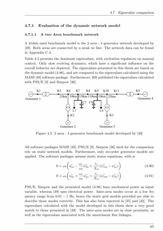
4.7 Eigenvalue comparison
4.7.1 Evaluation of the dynamic network model
4.7.1.1 A two Area benchmark network
A widely-used benchmark model is the 2 area - 4 generator network developed by
[49]. Both areas are connected by a weak tie line. The network data can be found
in Appendix C.4.
Table 4.3 presents the dominant eigenvalues, with excitation regulators on manual
control. Only slow evolving dynamics, which have a significant influence on the
overall behavior are depicted. The eigenvalues presented in this thesis are based on
the dynamic model (4.86), and are compared to the eigenvalues calculated using the
MASS [49] software package. Furthermore, [69] published the eigenvalues calculated
with PSS/E [9] and Simpow [36].
Figure 4.5: 2 area - 4 generator benchmark model developed by [49]
All software packages MASS [49], PSS/E [9], Simpow [36] used for the comparison
rely on static network models. Furthermore, only six-order generator models are
applied. The software packages assume static stator equations, with is
0 = ωb
(urqs −
ωrωbψrds +
rsXls
(ψrmq − ψrqs))
(4.90)
0 = ωb
(urds +
ωrωbψrqs +
rsXls
(ψrmd − ψrds)). (4.91)
PSS/E, Simpow and the presented model (4.86) have mechanical power as input
variable, whereas [49] uses electrical power. Inter-area modes occur at a low fre-
quency range from 0.01 − 1 Hz, hence the static grid models provided are able to
describe those modes correctly. This has also been reported in [35] and [42]. The
eigenvalues calculated with the model developed in this thesis show a very good
match to those presented in [49]. The inter-area modes are in close proximity, as
well as the eigenvalues associated with the amortisseur flux linkages.
65

4 Dynamic Security
Table 4.3: Eigenvalue comparison of a 2 area network
PSS/E Simpow MASS EVs of (4.86) Dominant[49] p. 815 States
0.32 0 -0.001 ± j0.002 -0.025 ± j5.79-0.106 0 -0.096 -0.136
-0.151 ± j3.41 -0.152 ± j3.42 -0.111 ± j3.43 -0.122 ± j4.09-0.606 ± j6.74 -0.661 ± j6.64 -0.492 ± j6.82 -0.458 ± j8.62-0.619 ± j6.94 -0.678 ± j6.84 -0.506 ± j7.02 -0.472 ± j8.08
-0.217 -0.1 ± j0.069 -0.117 -0.235-0.225 -0.191 -0.265 -0.265
-0.25 ± j0.21 -0.210 -0.276 -0.291-2.93 -3.6 -3.428 -2.299-3.85 -5.1 -4.139 -3.202-5.19 -8.04 -5.287 -4.788-5.21 -8.11 -5.303 -4.856-28.43 -34.12 -31.03 -10.24 ± 376.79
ψdq-29.92 -35.01 -32.45 -10.81 ± j376.79
-33.32 -36.02 -34.07 -13.55 ± j16974ζ
-34.71 -37.48 -35.01 -13.47 ± j17728-35.67 -37.48 -36.02 -13.25 ± j17753
-17.29 ± j28984-17.25 ± j29006-17.28 ± j29738-17.23 ± j29760
-21.33ψkd
-21.47-22.54-22.56
-25.04 ± j7781ζ
-25.04 ± j7027-28.50
-29.50 ± j376.82ψdq
-30.10-35.94-36.09
66

4.7 Eigenvalue comparison
As deduced in [49] the formulation used by MASS [49] and Simpow [36] use absolute
changes in machine rotor speed and angle as state variables, which create two zero
eigenvalues. One of the zero eigenvalues is caused by the lack of uniqueness of
the absolute rotor angle used. The rotor angle is described only in dependence
of internal generator variables, assuming a constant network frequency. However,
since the network is not connected to an infinite bus, the correct rotor angle is
calculated with
∆θi = ωi − ω (4.92)
= ωi − 1
Hsum
n∑j=1
Hjωj , (4.93)
where ω is the average system frequency, Hj is the inertia constant of generator j
and Hsum =∑Hj .
The second zero eigenvalue can be eliminated, if a speed governor is included or the
speed deviations are measured with respect to a reference machine. [69] suggests
that also the first and second entry of the eigenvalues calculated by PSS/E are
caused by the phenomena mentioned above. This is also validated by time-domain
simulations. Both cases are addressed in the presented model (4.86). Consequently,
the results of the reviewed commercial programs need to be interpreted with care,
if no excitation regulator or speed governor is included.
The additional eigenvalues (indicated in red), which do not occur in MASS [49],
Simpow [36] or PSS/E [9] can be traced back to the additional states used in
(4.86).
The relative participation of state variables and eigenvalues can be deduced with
the help of sensitivity analysis.
sen(i, j) = Vsys(i, j) ·Wsys(j, i) (4.94)
where Vsys,Wsys are the left- and righthand eigenvectors of the overall system (4.86).
(4.94) gives the sensitivity of eigenvalue λi. sen is a n× n matrix, where columns
are associated with eigenvalues and rows are associated with state variables. Large
values of (4.94) indicate a strong coupling, whereas small values indicate a weak
coupling of state variables with the corresponding eigenvalues. Eigenvalues with
frequencies of j376 are associated with ψdq, whereas frequencies higher than j5000
are associated with network dynamics.
67

4 Dynamic Security
4.7.1.2 5 Area benchmark network
The second assessed benchmark network has 14 generator groups, 59 busbars and
5 SVCs. The benchmark network is a contribution to the IEEE Benchmark Sys-
tems for Stability Controls Task Force [76]. The network data can be found in
Appendix C.5.
It was developed to demonstrate the ability of small-signal analysis and the design
of multi-machine controllers. The network has low frequency inter-area modes as
well as high frequency local modes. The test-bed includes 6 load cases, in order
to evaluate the proposed control method for several load scenarios. Each genera-
tor group is a generation equivalent representing a power station of 2 to 12 units.
Furthermore, high order excitation models are included.
The assessed benchmark grid has long lines and also includes shunt capacitors
and reactor banks. Hence, the eigenvalues from (4.25) and (4.26) are close to the
imaginary axis.
The quoted load cases 1 and 6, represent a high load and a moderate load scenario.
The eigenvalues and transient behavior are compared and discussed. As depicted
in Table 4.4 load case 6 has only 65 % of the energy demand compared to load case
1. Consequently, the number of generator units online, is significantly lower, which
also affects the total inertia of the network.
Table 4.5 shows the eigenvalues of both load cases including the dominant state
participation. Load case 1 and load case 6 represent unstable systems, without
dampening controllers. Furthermore, load case 6 has greater negative dampening.
Similar, to the 2 area network presented in Chapter 4.7.1.1, low frequency oscil-
lations are influenced by the states ω and the flux per second ψ in the majority
of modes. However, since the 5 area benchmark network is equipped with reactor
banks, which create additional modes very close to the imaginary axis. Those modes
have dominant state participation from network states ζ and no significant partic-
ipation from generators. The modes are significant for the system behavior and
do not occur with static grid models. Apart from modes created by reactor banks,
dominant state participation of network states occur from eigenvalues smaller than
−3.3.
Table 4.4: Overview of two load cases provided by [20]
Load Case 1 Load Case 6
22.3 GW 14.63 GW Total demand P5.5 GVar 0.4 GVar Total demand Q
62 40 Generator units932 MWs 589 MWs Hsum
68

4.7 Eigenvalue comparison
REF: D:\SAS_Rev3\IEEE_SAS_Report_Rev3\Simplified_14-Gen_System_Rev3.fm 6 of 4519 July 2010 9:32 am © The University of Adelaide
Figure 1 Simplified 14-generator, 50 Hz system.
BPS_2
ASVC_2
SVC
SVC
SVC
NPS_5
MPS_2
EPS_2
VPS_2
HPS_1
RSVC_3
LPS_3
SSVC_5
PSVC_5
PPS_5
T PS_5
TPS_4
CPS_4
SPS_4N_SVC
GPS_4
BSVC_4
YPS_3
SVC
SVC
SVC
309
102
311
305
314 313 312 302
301306
303
304307308
315101
217
216
214
215
213
204
210
212
209
202208
211
203
207201
206
205
416
415
414
413
410
411
412
409
408
405
407 404
406
403
402
401
310
509
503506
508
507
505502
504
501
AREA 4
AREA 2
AREA 3
AREA 5
AREA 1
Figure 4.6: Topology of the 5 area benchmark network developed by [20]
69

4 Dynamic Security
Table 4.5: Eigenvalue comparison of a 5 area network calculated with (4.87)
Case 1 Dominant Case 6 DominantStates States
0.183 ± j8.41ω
0.455 ± j10.41ω0.04 ± j5.69 0.156 ± j7.13
-0.134 ± j6.22 -0.0005 ± j8.05-0.143 ± j314.16 ζ -0.13 ± j314.16 ζ-0.161 ± j7.13 ω -0.143 ± j7.83 ω
-0.236 ψ -0.218 ψ-0.234 ± j314.16 ζ -0.221 ± j314.16 ζ
-0.247ψ
-0.233
ψ
-0.262 -0.246-0.282 -0.279-0.321 -0.28-0.323 -0.304
-0.338 ± j0.01 -0.316-0.349 ± j0.03 -0.318
-0.388 -0.332-0.407 -0.338
-0.435 ± j12.59 ω -0.351-0.46
ψ-0.364
-0.486 -0.382-0.549 -0.493± j13.51 ω-0.681 -0.504
ψ-0.772 -0.504-0.802 ± j15.15 ω -0.586
-0.831ψ
-0.88 ± j314.16 ζ-0.83 -0.895 ψ-0.913 -0.914 ± j15.71 ω
-0.951 ± j314.56ζ
-0.96 ψ-3.316 ± j14569 -3.316 ± j14569 ζ
70

4.7 Eigenvalue comparison
Dampening controllers need to show good performance for several operating condi-
tions. The eigenvalues of load case 1 and 6 can be used to specify the robustness
requirements of a control system. Fig. 4.7 shows the singular values of both load
cases. Computed are the input of generator BPS 2 located in area 2 versus all model
outputs. The resonant frequency changed considerable comparing case 1 and case
6 especially in the frequency range of 5 - 10 rad per second.
100 101 102
−50
0
50
Frequency in rad/s
SingularValues
indB Case 1
Case 6
Figure 4.7: Singular values of case 1 and case 6 calculated with (4.87)
71

72

Chapter 5
State Estimation
For monitoring purposes state estimators have become an invaluable asset. Phase
measurement units (PMUs) have the ability to improve the quality of estimators,
since the transfer rate is higher than in traditional measurement systems. Moreover,
the estimation problem becomes a linear problem as voltage magnitude and angle
are measured. With the exact knowledge of the grid state, voltage stability and
low frequency oscillations can be detected and appropriate countermeasures may
be initiated. Most of the advanced control schemes assume the knowledge of the
state variable x, in case the state variable is not measured it is estimated using an
observer structure as proposed in the following section.
5.1 Observer
With the introduction of PMUs it is possible to track dynamic incidents of power
systems. PMUs measure voltage and current phasors. Depending on the proposed
model structure the measurements are interpreted as inputs or outputs of the model.
The observer is able to estimate all states x of the process model developed in
Section 4.2, if the observability criterion is fulfilled. The state equations are
x = A x+B u (5.1)
y = C x (5.2)
with the given measurements y and input variables u. The observer includes a model
of the process which makes it possible to predict the estimated state variables x with
the given input variables. y = C x allows the estimation of the output variables.
y is then compared to the process measurements y. The observer gain L will
compensate the error y − y and x will converge to x . One method for an observer
synthesis is to solve the Riccati equation
AX + X AT − XT CT S−1 C X + Q = 0, (5.3)
73

5 State Estimation
C
L
ru ΒxΑ x x
yy
Nonlinear System
y
r
u
Observer
yu)f(x,x u)g(x,y
Figure 5.1: Observer structure
for X. X needs to be positive definite, which in this context is defined as X > 0.
Where Q and S are positive definite weighting matrices minimizing the objective
function
J =
∫ ∞−∞
u(t)TS u(t) + x(t)TQx(t) dt . (5.4)
Solving the Riccati equation after X leads to the observer gain
L = (S−1 C XT )T . (5.5)
The deployed network model as derived in equation (4.29) is
[uF0
]=
[LF 0
0 −E
]︸ ︷︷ ︸
MF
[iFζ
]•+
[RF CFBF AN
]︸ ︷︷ ︸
AF
[iFζ
](5.6)
The network model is rearranged into state space form[iFζ
]•= −M−1
F AF
[iFζ
]+M−1
F
[uF0
]. (5.7)
In the following uF is defined as input and iF as measured output, which makes
iF =[E 0
] [ iFζ
]. (5.8)
74

5.2 Results
Estimated are the state variables[iF ζ
]T. The nodal voltages udq are calcu-
lated with the help from (4.25).
5.2 Results
To prove the capabilities of the observer for monitoring purposes, the two area
benchmark network according to Section 4.7.1.1 was chosen. The specific network
data can be found in the Appendix. Every feeding node, i.e. nodes 1 to 4, has
a phasor measuring unit. In practice the data would be transmitted to a data
concentrator, whose data would be available to the observer. Simulation results
for the given network and a 3-phase short circuit with a duration of 150 ms at
node 8 are depicted in Fig. 5.2. The estimates of the observer are compared with
the simulation results created with a commercial power system software package.
Fig. 5.2 depicts the magnitude and phase voltage of the estimated nodal voltages.
During the short circuit the simulation and the estimates have a discrepancy. This
is due to the fact that the estimator has no knowledge about the short circuit. It
only has sensory input from PMUs located at great distance to the node where the
short circuit occurs. Immediately after the fault is resolved, angle and magnitude of
the simulated and estimated voltages are almost identical. Although the ability to
estimate the voltage evolution after a fault is imperative to assess voltage stability
and inter-area oscillations, the presented results of the estimated voltage magnitude
during transient events have not been accomplished before. A procedure to estimate
the state variables of synchronous generators has been presented in [83].
75

5 State Estimation
0 1 2 3
1
1.2
|UK
5|
Absolute Value
0 1 2 3
0.91
1.1
|UK
6|
0 1 2 30.8
1
|UK
7|
0 1 2 30.2
1
|UK
8|
0 1 2 30.8
1
|UK
9|
0 1 2 30.8
1
|UK
10|
0 1 2 3
1
1.2
Time in sec.
|UK
11|
0 1 2 3-1.1
-1-0.9
U
K5
Phase
0 1 2 3
-1.2-1.1
-1
U
K6
0 1 2 3
-1.2
-1
UK
7
0 1 2 3-2.2
-1.2
U
K8
0 1 2 3
-1.5-1.4-1.3
U
K9
0 1 2 3
-1.4-1.3-1.2
U
K10
0 1 2 3-1.3-1.2-1.1
Time in sec.
U
K11
Estimation
Orignial
Figure 5.2: Absolute value and phase of nodal voltages of a 2 area network, after 1sec. a short circuit occurs at node 8
76

Chapter 6
FC-MPC to improve dynamic stability
6.1 Motivation
This chapter presents an integral control strategy that integrates data from phase
measurement units to damp inter-area oscillations. The proposed distributed model
predictive control (dMPC) method has one control unit for each controllable device
(Generators, FACTS, HVDC) and coordinates their behavior after a fault. Each
unit is designed by applying a systematic controller synthesis. The distributed MPC
has a significantly improved performance compared to a standard power system
stabilizer.
Power system stabilizer (PSS) methods can be divided into damping torque, fre-
quency response and eigenvalue techniques. In [22] the damping torque concept
has been developed, whereby the proportionality between electrical damping torque
and speed perturbations is applied to damp the system. PSSs based on the damp-
ing torque concept tend to perform worse in field tests as compared to results
attained by analysis. This can be traced back to the interaction of PSSs and has
been observed for local and inter-area modes [21]. Multiple-input and multiple-
output (MiMo) models describe interaction system coupling. The resulting MiMo
controllers account explicitly for couplings of the system and achieve an optimal
control, considering all generators and power converters. Especially complex, cou-
pled systems with several in- and outputs perform significantly better with MiMo
control. Model predictive control is an advanced control method and in its classical
form is a central MiMo controller. Central controllers are not applicable due to the
spatially distributed nature of power systems. However, [65] developed distributed
MPC variants, which can be applied in a power system setting [74].
In 2000 Bonneville Power Administration was the first TSO to put a wide area
measurement system (WAMS) into service, consisting of phase measurement units
(PMUs) and a data concentrator. PMUs measure the absolute value and angle of
voltage and currents with very high accuracy and sample time. The measured data
is transmitted to the data concentrator, where data packages are synchronized and
77

6 FC-MPC to improve dynamic stability
made available. WAMS are in application in many states of the USA and Canada.
Furthermore, Europe, China and India have WAMS in operation.
The existing electrical power systems in Europe and North America have multiple
monitoring systems at transmission level. However, the control systems of power
plants rely only on local measurements. The control law is therefore not based on
the overall grid state, but only on the measured terminal voltages and frequency
deviations. Assuming a wide area measurement system, a controller which relies
not only on local measurements, but also on several PMU measurements, becomes
feasible.
Control design methods for fast acting controllable devices (Exciters, HVDC, FACTS)
need dynamic network equations to describe the behavior satisfactorily if these
devices are electrically close to each other. A model including dynamic network
equations is developed in Chapter 4.
The distributed MPC presented here is based on this model and inherently considers
the interaction between generators, power converters and grid dynamics correctly.
Furthermore, dMPC control is based on MPC control, which is a MIMO controller
with the described advantages.
Dynamic stability is especially critical in low inertia systems. Examples are island
systems and wind farms where the generation is supplied from power converters [79].
Scenarios where only low inertia is available are for instance the island operation
of large AC networks after tripping of a crucial component and the black start of
a power network. Consequently, advanced control schemes were applied first in
island systems. For instance ABB [67] and Hitachi [45] are working on advanced
protection and control schemes, that integrate remote signals from WAMS.
The dMPC control strategy described here achieves results very close to the global
optimum for the following reasons. Each distributed control unit considers all
state variables for the optimization. Every controller has a global objective and
considers the couplings of the overall system. The controller relies primarily on
local measurements and uses global measurements when available.
6.1.1 Literature Review
[64] and [62] propose a robust approach using linear matrix inequalities based on
pole placement and H∞, respectively. The controllers are robust against influence
from neighboring plants resulting in a decentralized controller. [52] is using mixed
H2/H∞ synthesis controlling HVDC and FACTS devices. [38] integrates wide area
dynamical information into the control system based on a selective modal perfor-
mance index, damping inter-area modes. [59] develops a PSS based on fuzzy control
using remote signals. [61] as well as [12] develop a central control scheme improving
78

6.1 Motivation
the PSS performance considering signal transmission delays. [18] presents a central
MPC coordinating several HVDC devices. [3] gives an overview on published su-
pervisory PSS. [73] formulates dMPC strategies and applies control methods to the
automatic generation control problem. [73] shows that the performance benefits
obtained from MPC can be realized through dMPC for large scale systems.
This chapter is organized as follows: The implemented control scheme with dis-
tributed control units and one data concentrator state estimator is explained. First
followed by a description of the MPC strategy developed. The potential of the
dMPC controller in comparison to pure PSS dampening is demonstrated with sim-
ulation results for 2 and 5 area networks.
6.1.2 Controller Structure
A distributed control method for the nonlinear process of generation units and SVC
connected over a network, is introduced as shown in Fig. 6.1. The control method
relies primarily on local measurements. This thesis uses standard PSS as presented
in [49], [20] as local control method, any decentralized method is applicable.
Network
Generators
udq
us2
Data Concentrator
State Estimator
xest
xestus1
dMPC 2
PSS 2
dMPC 1
PSS 1
Figure 6.1: Block diagram of a power system represented by 2 generators andnetwork controlled by a multi-machine controller structure
79

6 FC-MPC to improve dynamic stability
The applied PSS methods use the rotor speed deviation as input and provide a
stabilizing signal as output. An implementation without PSS is presented in [82].
The corresponding network has a WAMS available, which measures U , I, ω at
several locations throughout the grid. As indicated in [23], it is advantageous to
position the PMUs at the feed-in nodes involved in frequency and/or voltage control.
Consequently, every major feed-in node has one PMU available.
The measurements are transferred to the data concentrator, where data synchro-
nization is established. The measurements are used to estimate the network state
variables ζ, as introduced in Chapter 5. The state variables of all controllable
devices (generators, SVC) can be calculated/estimated directly at the device and
need to be transferred to the data concentrator. The number of state variables can
be reduced further by using model reduction methods [66]. The synchronized and
assembled state variables are transferred to all participating controllable devices as
a global signal. The distributed MPC developed provides an additional stabilizing
signal, which corrects the PSS output with the help of the global signal. One dMPC
controller is implemented for each controllable device and is located, as for the PSS,
directly at the device. The dMPC works with sample times up to 1 second.
The control loops of a conventional power plant are depicted in Fig. 6.2 in more
detail. The plower plant control consists of two main loops, one for the excitation
and one for the torque control. Both control loops remain intact in comparison to
the conventional implementation. The resulting stabilizing signal us attained from
PSS and dMPC output is used as a set point update of the excitation control. The
absolute value of the voltage and the rotor speed of the generator are measured.
The excitation voltage ufd and the torque Mm are inputs to the generator.
Turbine & Regulators
Excitation dMPC 2
PSS|u|
w
uxf
Mm
xest
Figure 6.2: Block diagram of a conventional control system including PSS anddMPC
80
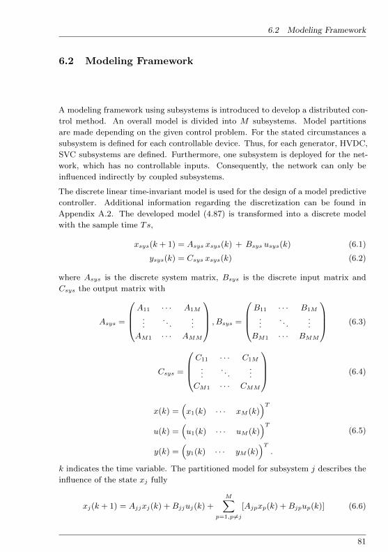
6.2 Modeling Framework
6.2 Modeling Framework
A modeling framework using subsystems is introduced to develop a distributed con-
trol method. An overall model is divided into M subsystems. Model partitions
are made depending on the given control problem. For the stated circumstances a
subsystem is defined for each controllable device. Thus, for each generator, HVDC,
SVC subsystems are defined. Furthermore, one subsystem is deployed for the net-
work, which has no controllable inputs. Consequently, the network can only be
influenced indirectly by coupled subsystems.
The discrete linear time-invariant model is used for the design of a model predictive
controller. Additional information regarding the discretization can be found in
Appendix A.2. The developed model (4.87) is transformed into a discrete model
with the sample time Ts,
xsys(k + 1) = Asys xsys(k) + Bsys usys(k) (6.1)
ysys(k) = Csys xsys(k) (6.2)
where Asys is the discrete system matrix, Bsys is the discrete input matrix and
Csys the output matrix with
Asys =
A11 · · · A1M
.... . .
...
AM1 · · · AMM
, Bsys =
B11 · · · B1M
.... . .
...
BM1 · · · BMM
(6.3)
Csys =
C11 · · · C1M
.... . .
...
CM1 · · · CMM
(6.4)
x(k) =(x1(k) · · · xM (k)
)Tu(k) =
(u1(k) · · · uM (k)
)Ty(k) =
(y1(k) · · · yM (k)
)T.
(6.5)
k indicates the time variable. The partitioned model for subsystem j describes the
influence of the state xj fully
xj(k + 1) = Ajjxj(k) +Bjjuj(k) +
M∑p=1,p 6=j
[Ajpxp(k) +Bjpup(k)] (6.6)
81

6 FC-MPC to improve dynamic stability
where Ajj , Bjj is the effect of local subsystem variables and Ajp, Bjp the effect of
interconnected subsystems.
The output equation is defined with
yj(k) =
M∑p=1
Cjpxp(k). (6.7)
In comparison traditional PSS are decentralized control methods, relying only on
local subsystem variables. Any influence of interconnected subsystems is not con-
sidered in the design process. A decentralized model is defined with
xj(k + 1) = Ajjxj(k) +Bjjuj(k). (6.8)
6.3 Feasible Cooperation MPC
[73] developed a feasible cooperative model predictive controller. The controllers
are distributed and can be located close to the actuators. In order to apply a
distributed, predictive control approach the central MPC as described in Chapter
2 needs to be adapted.
6.3.1 Model manipulation
Analogously to the central MPC introduced in Chapter 2, the distributed MPC is
derived from (6.8), which is equal to the first prediction time step
xj(k + 1) = Ajjxj(k) +Bjjuj(k) +M∑p6=j
[Ajpxp(k) +Bjpup(k)]. (6.9)
The second time step with k ⇒ k + 1 is
xj(k+2) = Ajjxj(k+1)+Bjjuj(k+1)+
M∑p 6=j
[Ajpxp(k+1)+Bjpup(k+1)]. (6.10)
82

6.3 Feasible Cooperation MPC
Substituting xj(k + 1) with (6.9) leads to
xj(k + 2) = A2jjxj(k) +
(AjjBjj Bjj
)( uj(k)
uj(k + 1)
)
+
M∑p 6=j
[AjjAjpxp(k) +Ajpxp(k) +
(AjjBjp Bjp
)( up(k)
up(k + 1)
)],
(6.11)
where (6.9) defines the first time step for sub-model j and (6.11) the second time
step for sub-model j. The formulation for N time steps and one subsystem is given
with
xj = Ejj uj + fjjxj(k) +
M∑p 6=j
Ejpup + fjpxj(k) + gjpxp, (6.12)
where
Ejp =
Bjp 0 · · · · · · 0
AjjBjp Bjp 0 · · · 0...
. . .. . .
. . ....
AN−1jj Bjp · · · · · · · · · Bjp
,
fjp =(Ajp AjjAjj · · · AN−1
jj Ajp)T,
gjp =
0 0 · · · · · · 0
Ajp 0 0 · · · 0...
. . .. . .
. . ....
AN−2jj Ajp AN−3
jj Ajp · · · · · · 0
.
xj and u are defined with
xj =(xj(1) . . . xj(N)
)T, (6.13)
uj =(uj(1) . . . uj(N)
)T. (6.14)
83

6 FC-MPC to improve dynamic stability
E and f have the same structure as Su, Sx of the central formulation. However,
the presented distributed formulation is consistent with the subsystems defined in
Section 6.2. Converting (6.12) leads to
xj −M∑p6=j
gjpxp = Ejj uj + fjjxj(k) +
M∑p 6=j
Ejpup + fjpxj(k). (6.15)
The model for N time steps and the overall model is
A
x1
...
xM
= E
u1
...
uM
+ Gx(k) (6.16)
x1
...
xM
= A−1E︸ ︷︷ ︸E
u1
...
uM
+A−1G︸ ︷︷ ︸f
x(k) (6.17)
where
A =
I −g12 · · · −g1M
−g21 I −g2M
.... . .
. . .. . .
−gM1 −gM2 · · · I
,
E =
E11 · · · E1M
.... . .
...
EM1 · · · EMM
,
G =
f11 · · · f1M
.... . .
...
fM1 · · · fMM
.
The central formulation (2.5) represents a model with prediction horizon and x =
f(x(k), u). (6.17) assembles the same model including prediction horizon, but also
preserves subsystem boundaries.
Hence:
xj = fjjxj(k) + Ejj uj +
M∑p6=j
fjpxp(k) + Ejpup (6.18)
84

6.3 Feasible Cooperation MPC
where xj gives the model predictive equation set for subsystem j and N time steps
only in dependence of x(k) and u, which shall be used for the optimization. The
matrices E and f are defined by (6.17).
Since the existing problem is an output regulator problem with the control variable
ω, the output equation over the prediction horizon is needed. The output yj is
coupled with all subsystems, but is independent of the prediction step.
yj =
M∑j=1
Cjixi (6.19)
with
Cji =
Cji · · · 0
.... . .
...
0 · · · Cji
. (6.20)
6.3.2 Objective Function
For each subsystem j and iterate it the control variable is defined with uitj . Each
MPC controller calculates the optimal actuating variable considering the objective
function
Vj(k) =
M∑s=1
ωjs[[ys(k)− τs(k)]T Qs(k) [ys(k)− τs(k)] + us(k)TRs(k)us(k)
](6.21)
τs is the set point for each subsystem and Q, R are positive-definite weighting
matrices. Cooperation of the dMPC controllers is needed to achieve system wide
objectives. Therefore, the overall system influence and the objectives of all subsys-
tems are incorporated into the cost function Vj of subsystem j. wjs is a weighting
term for each subsystem with∑s wjs = 1 and wjs > 0. wjs defines the considera-
tion of neighboring subsystems in the controller design. wjj = 1 only optimizes the
controller with respect to the own subsystem, whereas wjs = 1M, ∀ s optimizes the
controller with respect to all subsystems in equal weight.
A quadratic cost function was taken for this example. The matrix Cji is defined
with (6.20). Substituting (6.18) into (6.19) and the resulting equation into (6.21)
formulates a PQ-problem. In the following the time variable (k) is dropped for
simplicity.
Vj = minuj
1
2uTj Φj uj +
KMPC,jx+∑p 6=j
WMPC,jpuit−1p
T
uj + const (6.22)
85

6 FC-MPC to improve dynamic stability
The PQ-problem of controller j is given in (6.22). (6.22) has a quadratic term
penalizing local control variables uj , additionally the product of x · uj and uit−1p · uj
is penalized. Here x is the overall state vector and uit−1p are control variables of
neighboring subsystems which are not optimization variables. Vj is only optimized
for uj .
To calculate the optimal solution for a trajectory uopt,j , equation (6.22) is differen-
tiated with respect to uj and set to zero.
dVjduj
=
KMPC,jx+∑p6=j
WMPC,jpuit−1p
T
+ Φj uj = 0
which leads to the optimal control law:
uopt,j = −Φ−1j
KMPC,jx+∑p6=j
WMPC,jpuit−1p
T
(6.23)
After considerable work Φj , KMPC,j and WMPC,jp are obtained
Φj =
[ωjjRj +
M∑s=1
[M∑i=1
(CsiEij)TωjsQs
M∑i=1
(CsiEij)
]]
KMPC,jx =M∑s=1
M∑i=1
(CsiEij)TωjsQs
(M∑i=1
Csi
M∑p=1
[fipxp
]− τs
)
∑p6=j
WMPC,jpup =
M∑s=1
M∑i=1
(CsiEij)TωjsQs
M∑i=1
Csi
M∑p6=j
[Eipu
it−1p
]− τs
6.3.3 Implementation
The implemented dMPC procedure does not explicitly account for constraints such
as the rate of change or saturation effects. Therefore, the dMPC controller is
deducible with an analytical solution as shown in (6.23). Hence, a static control
matrix can be calculated, which has several inherent advantages.
• The optimization can be calculated offline
• Stability and robustness analysis is possible
86

6.3 Feasible Cooperation MPC
In order to penalize input and state changes it is useful to transform the system with
∆u = u−u0 and ∆y = y−y0. Thus, ∆u are the new optimization variables and ∆x
the newly obtained state variables after the transition to ∆-values. The set point
of the operation point can be reached with ∆τ = 0. The presented dMPC method
is an iterative approach and assumes communication of dMPC controllers. The
control law (6.23) is dependent on the input variables of neighboring subsystems.
The distributed controller is applying values from the previous iteration ∆uit−1p ,
consequently assumptions are necessary regarding their initial value ∆u0p at iterate
it = 1. The initial value ∆uit−1p is assumed to be zero. Simulation results show
that the same controller performance is attained if ∆uit−1p (k) = ∆uit−1
p (k − 1). In
order to allow several iterations, the data transfer between controllers needs to be
considerably faster than the sample time Ts. With a high number of controllers
the requirements to transfer rate and data volume would be significant. The imple-
mentation presented stops after the first iteration to avoid these obstacles.
6.3.4 Simulation Results - 2 Area Network
A 4 generator benchmark model according to [49] is chosen to demonstrate the
performance of the developed dMPC approach. Fig. 6.3 depicts a detailed example
of the control structure and data transmissions for the benchmark model. Each
feed-in node is equipped with a PMU. The PMU data is transmitted through a
data concentrator to the state estimator.
2 4
87 9
G2 G4
T2 T4
L7 L9G3
T3
1
G1
T1
3
dMPC1
dMPC2 dMPC4
dMPC3
Data
State
Concentrator
EstimatorPMUustabCommunication Ts (1s)
5 6 10 11
Figure 6.3: Two area network with dMPC control, communication, data concentra-tor and state estimator
87

6 FC-MPC to improve dynamic stability
A Kalman-Bucy Filter is used for the estimation as introduced in Chapter 5. By
applying (4.29), the filter estimates all network state variables ζ. As indicated in
Fig. 6.6b all state variables, except for those xj available locally, are transferred to
the corresponding dMPC controller. The procedure of data transmission and state
estimation is time consuming. Thus, the sample time is Ts = 1s. Each generator is
equipped additionally with a MB-PSS IEEE type PSS4B, as defined in Appendix
B. The PSS is not depicted in Fig. 6.3 for simplicity. The stabilizing signal ustabfrom each dMPC unit is added to the PSS output. The PSSs compensate for the
slow transfer rate of the WAMS.
0 1 2 3 4 5 6 7 80.98
0.99
1
1.01
T ime in s
ωinp.u
dMPC+PSSPSS
Figure 6.4: ω of dMPC controlled system in comparison to PSS after a 500 msshort circuit
0 1 2 3 4 5 6 7 8
0.9
1
1.1
1.2
T ime in s
|U|inp.u.
dMPC+PSSPSS
Figure 6.5: |U| of dMPC controlled system in comparison to PSS after a 500 msshort circuit
Fig. 6.4 shows the rotor speed and Fig. 6.5 shows the magnitude of the terminal
voltages of all generators. The simulation results created with the dMPC procedure
(continuous line) are compared to a MB-PSS IEEE type PSS4B according to IEEE
Std 421.5 (dotted line). After one second of simulation time a 3-phase short circuit
occurs at node 8 for 500 ms. dMPC and PSS are able to stabilize the system.
88

6.3 Feasible Cooperation MPC
However, as depicted in Fig. 6.4 and 6.5, the time evolution of the rotor speed
and voltage magnitude of the dMPC controlled system are significantly better than
the PSS controlled system. The maximum rotor speed deviation of the dMPC
controlled system is 0.01 p.u. compared to 0.02 p.u. for the PSS controlled system.
After just 5 s the terminal voltage of the dMPC controlled system is close to the
set point. The PSS needs 5.5 s to damp the oscillation, and needs 28.5 s to return
the terminal voltage back to its set point.
6.3.5 Simulation Results - 5 Area Network
After successful evaluation of the control method in a 2 area network setting, the
control method is evaluated and discussed in a larger network. The system becomes
more complex with the rising number of generators and nodes. This effectively
entails a rising number of modes and a rising number of control variables. The 5
area network, already shown in Fig. 4.6, includes generators and SVCs as actuators,
which are able to control the power flow.
SVC
SVC
SVC
SVC
SVC
SVC(a) Topology of the 5 area benchmark net-work. The simulated scenarios are short cir-cuit of 150 ms (rectangle), loss of generationunit (triangle) and loss of a load (circle)
gg + s-g
s-s
est
est
g
s
(b) Control scheme with distributed controlunits, one data concentrator, state estimator∀ g = 1 .. G and ∀ s = 1 .. S, where G is thetotal number of generators and S is the totalnumber of SVCs
Figure 6.6: Overview of the 5 area network and the implemented control approach
89

6 FC-MPC to improve dynamic stability
Three contingencies are considered in the 5 area network. As illustrated in Fig. 6.6a
considered are: a short circuit at bus 206 (area 2) of 150 ms, the loss of a generation
unit at bus 501 (area 5) and the loss of a load at bus 409 (area 4). The control
structure of the dMPC for the 5 area network is shown in Fig. 6.6b, which is a
simplified scheme of Fig. 6.3. A PMU is located at each generator and SVC feed-in.
The data is transferred to the data concentrator and state estimator. The sample
time of each dMPC is Ts = 1s; i.e. each controller receives a refreshed estimation
of the state variables xest. The optimization horizon is N = 5. All generators have
a PSS. The distributed MPC developed provides an additional stabilizing signal,
which corrects the PSS output with the help of the global signal. In addition the
set points of the 5 SVCs deployed at the network are updated with the dMPC
controller output. Consequently, 14 dMPC controllers are located at power plants
and 5 dMPC controllers are responsible for SVCs.
6.3.5.1 Dynamic stability versus rotor angle stability
Eigenvalues describe the dampening behavior after a contingency and give infor-
mation on the oscillatory response. Small signal analysis is only valid around an
operation point. Rotor angle stability is not considered in small signal analysis. In
order to maintain rotor angle stability, θ of all generators needs to be smaller than
90 during stationary operation. Moreover, a rotor angle of all generators < 180
has to be preserved during transients in order to maintain synchronism. The low fre-
quency oscillations also excite rotor angle oscillations during transient operation. A
fast deactivation of the excited frequencies is in itself not of paramount importance
in power systems [62]. However with the thereby excited rotor angle oscillations and
a potential generator failure, a fast dampening with small rotor angle deviations
becomes very relevant.
In Chapter 4 load cases 1 and 6 are introduced and an eigenvalue comparison is
presented, leading to the following conclusion: The modes of case 6 are more weakly
damped and have a strong resonant frequency around 9 rad per second. On the
other hand, load case 1 represents a peak load condition, whereas load case 6 is a
moderate load condition. Therefore, the rotor angle reserve at case 1 is smaller than
in case 6. Load case 1 has a maximum rotor angle of θmax = 70 and a mean rotor
angle of θavg = 48, whereas load case 6 has a maximum rotor angle of θmax = 59
and a mean rotor angle of θavg = 45. Even though, load case 6 is dynamically less
stable, load case 1 is the more critical case, due to the small rotor angle reserve. For
load case 6 the PSS controlled network, has a similar performance as the dMPC
controlled network for all contingencies. In the following simulation results are
presented discussing load case 1.
90

6.3 Feasible Cooperation MPC
6.3.5.2 Short Circuit
The simulation results compare the developed dMPC scheme to PSS developed by
[20]. Fig. 6.7a and Fig. 6.7b depict the rotor angle of all generators in reference
to generator LPS3. Fig. 6.7c and Fig. 6.7d show the rotor speed of all connected
generators. The considered contingency first is a 3-phase short circuit at bus 206
of 150 ms. Due to the short circuit all areas lose steady state and the system
performs a transient response. The dMPC controlled system is stable, whereas
the PSS controlled system loses rotor angle stability after 5 seconds. The rotor
angle reserve for case 1 in area 5 is only 20. Even though the short circuit occurs
far away from area 5 the rotor angle oscillations of generators NFS5, TPS5 and
PPS5 lose synchronism. Hence, all generators located in area 5 are disconnected
from interconnected operation. The maximum frequency deviation of the dMPC
controller system is ∆ω = 0.023 p.u.
0 2 4 6 8 10-200
-100
0
100
Time in sec.
∆θ
(a) Rotor angle of dMPC controlled sys-tem after short circuit
0 2 4 6 8 10-200
-100
0
100
Time in sec.
∆θ
(b) Rotor angle of PSS controlled systemafter short circuit
0 2 4 6 8 10
0.97
1
1.02
Time in sec.
ωin
p.u.
(c) Rotor speed of dMPC controlled sys-tem after short circuit
0 2 4 6 8 10
0.97
1
1.02
Time in sec.
ωin
p.u.
(d) Rotor speed of PSS controlled systemafter short circuit
Figure 6.7: Simulation results of the 5 area network
91

6 FC-MPC to improve dynamic stability
The dMPC controlled system is able to preserve stability and after 7 seconds the
frequency of the system is equal to fN . The rotor angle oscillations of the dMPC
controlled system are significantly better damped.
6.3.5.3 Generator unit failure
A power plant in area 5 (NFS5) loses a generation unit, causing a power deficit
of 266 MW. Fig. 6.8a and Fig. 6.8b depict the rotor angle of all generators in
reference to generator LPS3. Fig. 6.8c and Fig. 6.8d show the rotor speed of all
connected generators. The contingency has a small impact on the system and only
a minor influence on neighboring areas. However, the PSS controlled system is not
able to stabilize the remaining generators and after 5 seconds the generators located
in area 5 lose synchronism.
0 2 4 6 8 10
-100
0
100
Time in sec.
∆θ
(a) Rotor angle of dMPC controlled sys-tem after generator unit failure
0 2 4 6 8 10
-100
0
100
Time in sec.
∆θ
(b) Rotor angle of PSS controlled systemafter generator unit failure
0 2 4 6 8 10
0.998
1
1.002
Time in sec.
ωin
p.u.
(c) Rotor speed of dMPC controlled sys-tem after generator unit failure
0 2 4 6 8 10
0.97
1
1.02
Time in sec.
ωin
p.u.
(d) Rotor speed of PSS controlled systemafter generator unit failure
Figure 6.8: Simulation results of the 5 area network
92
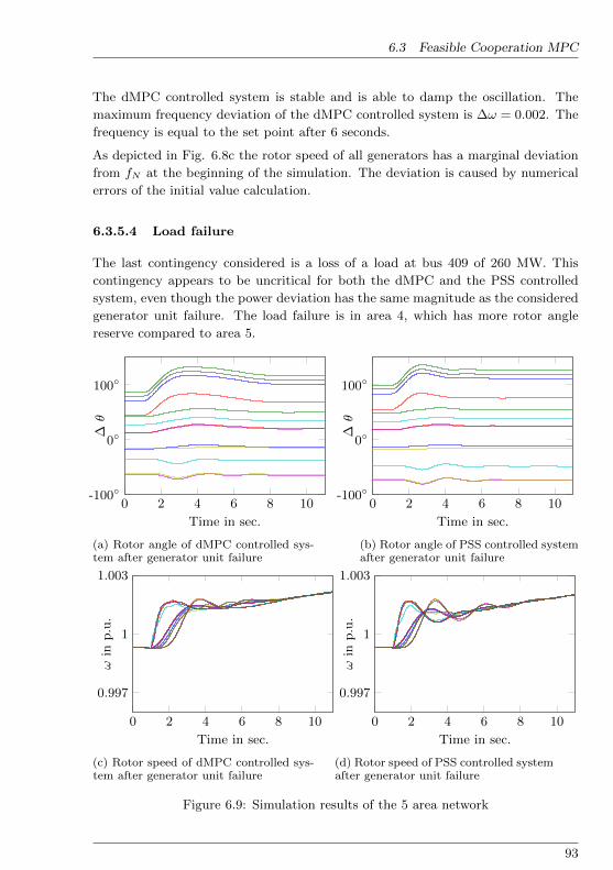
6.3 Feasible Cooperation MPC
The dMPC controlled system is stable and is able to damp the oscillation. The
maximum frequency deviation of the dMPC controlled system is ∆ω = 0.002. The
frequency is equal to the set point after 6 seconds.
As depicted in Fig. 6.8c the rotor speed of all generators has a marginal deviation
from fN at the beginning of the simulation. The deviation is caused by numerical
errors of the initial value calculation.
6.3.5.4 Load failure
The last contingency considered is a loss of a load at bus 409 of 260 MW. This
contingency appears to be uncritical for both the dMPC and the PSS controlled
system, even though the power deviation has the same magnitude as the considered
generator unit failure. The load failure is in area 4, which has more rotor angle
reserve compared to area 5.
0 2 4 6 8 10-100
0
100
Time in sec.
∆θ
(a) Rotor angle of dMPC controlled sys-tem after generator unit failure
0 2 4 6 8 10-100
0
100
Time in sec.
∆θ
(b) Rotor angle of PSS controlled systemafter generator unit failure
0 2 4 6 8 10
0.997
1
1.003
Time in sec.
ωin
p.u.
(c) Rotor speed of dMPC controlled sys-tem after generator unit failure
0 2 4 6 8 10
0.997
1
1.003
Time in sec.
ωin
p.u.
(d) Rotor speed of PSS controlled systemafter generator unit failure
Figure 6.9: Simulation results of the 5 area network
93

6 FC-MPC to improve dynamic stability
Additionally, area 4 is distant to area 5, hence the power unbalance has very little
influence on area 5. The frequency deviation is in both cases ∆ω = 0.0017. The
decay of the oscillation takes 7 seconds.
6.3.6 Discussion
Controller relying on remote signals have superior performance as compared to
decentralized PSS; the reviewed publications include many examples showing this.
The presented distributed controller significantly improves transient stability, in-
cluding angle stability. The controller explicitly considers control interaction through
the underlying process model which includes network dynamics and through the im-
plementation of a MiMo controller.
All reviewed approaches, except for [18], assume a time-continuous controller and
examine the robustness of the controller against communication delays up to 400ms.
The presented approach implements a time-discrete controller, explicitly considering
transfer/sample rates. The dMPC controller shows good performance for a sample
time of 1s for the 2 area network and the 5 area network, respectively. The assumed
sample rates are less demanding, i.e. more realistic, compared to the reviewed
approaches. Furthermore, central controller schemes such as [18] are vulnerable to
communication disturbances or SCADA failures. [81] has presented a central MPC
control scheme.
The approach presented here assumes a real-time communication interface, which
is able to provide the state variable xest every 1s. This chapter solves the control
problem through a distributed approach, but does not address the communication
problem. In general, control schemes are preferable which need as few measured
variables as possible. Several methods to reduce the estimation and communication
effort are available.
• Model reduction methods reduce the number of state variables and therefore
the communication needed. Since only a very limited range of the spectrum
is of interest, the number of state variables can be significantly reduced [62].
• A hybrid network model reduces the number of state variables and still con-
siders control interaction [42].
• The controllability analysis gives information on which controllers can damp
which modes most effectively. Furthermore, the observability analysis gives
information on which feedback signals are most conclusive [38]. Hence, not
all controllers need a global signal and the cooperating controllers need mea-
surements from only a few locations.
94

6.3 Feasible Cooperation MPC
• State estimators which rely on predictor-corrector methods are able to com-
pensate for sporadic communication delays. In case no up-to-date estimation
is available due to measurement failure, the predicted variables can be used.
• Robust dMPC implementations will improve control performance against
model errors and unmeasured subsystem influence
Note that a reduced system model may result in deteriorating control performance.
6.3.7 Conclusion
The chapter presents a novel approach to systematically integrate PMU-data and
coordinate a large number of hardware actuators (Generators, FACTS, HVDC).
The optimal trajectories for each control variable are calculated in order to damp
inter-area oscillations. Each controller complies with the global objective. Hence,
the dMPC approach has a dynamic performance close to a central MPC [74]. The
performance is significantly better compared to a PSS, and thus the dMPC approach
improves reliability and operational flexibility.
95

96

Chapter 7
Conclusion and Outlook
The focus of this thesis lies in the improvement of power system security with high
renewable energy sources (RES) in-feed. The first section within this thesis regards
the optimal operation of a diverse generation unit portfolio considering operating
ranges like transmission line and generation constraints during stationary operation.
Generation dispatch and redispatch strategies are developed. In order to integrate a
high share of RES, operational flexibility is imperative. Volatile RES challenge one
of the fundamental requirements of power system operation, namely the balance of
demand and supply.
In order to formulate an optimization problem, a modeling framework is introduced,
describing the diverse generation units and the power flow. This thesis presents for-
mulations for normal operation and operation after a contingency took place. The
optimization takes place over a prediction horizon, hence inter-temporal dependen-
cies like storage devices and generation ramping constraints are considered. In
addition, the optimization accounts for load and RES forecasts.
Since power systems are divided into several control areas with corresponding as-
signment of responsibilities, it is crucial to consider zoning within the problem
formulation. A cooperative optimization is presented in which several control ar-
eas attain a verified schedule. For each control area a player is introduced, with
the goal to create an iterative procedure which makes cooperation of control areas
possible. Each zone conducts its own optimization with inclusion of approximated
neighboring generation costs. The generation pattern load and RES feed-in fore-
casts are exchanged. Through an iterative approach, a solution close to the global
optimum is reached. Due to the high costs for storage and hot standby operation
of conventional power plants, grid operation needs to be as close as possible to the
global optimum.
The functionality is shown successfully using stressed 14 and 118 node systems. A
cross border dispatch with use of storage devices is realized to maintain a high share
of RES feed-in, while reducing overall dispatch costs.
97

7 Conclusion and Outlook
The second area addressed in this thesis is the transient operation of power systems.
Due to the rising numbers of RES and hesitant network reenforcement, transfer ca-
pacity reserves as well as total inertia decrease. Thus, the affected power systems
have poor transient behavior.
On the other hand controllable devices like generators, FACTS and HVDC located
through out the network are able to control the power flow and can improve the
transient behavior. In order to avoid cascading blackouts, dampening controllers
are implemented which are a significant part of this thesis. This thesis develops
dampening controllers improving the performance of local power system stabilizers.
In order to coordinate the behavior of the controllable devices a cooperative objec-
tive function is used, which optimizes each distributed controller towards a system
wide objective.
Furthermore, the distributed controllers are based on an overall network state pro-
vided by a dynamic state estimator. This development is also within the scope
of the presented thesis. The state estimator is also capable of estimating voltage
phase and absolute value of a network assuming a wide area monitoring system.
Control design methods for fast acting controllable devices (Exciters, HVDC, FACTS)
need dynamic network equations to describe the behavior satisfactorily if these de-
vices are electrically close to each other. This thesis implements a dynamic network
model from minimal order, which explicitly considers the control interaction phe-
nomenon. The developed small signal model is applied to control synthesis. Con-
sequently, the deployed dampening controllers avoid interaction. A high number
of controllable devices with dampening controllers is difficult to design, therefore a
systematic design approach is implemented.
The control scheme is successfully implemented for 11 and 59 node benchmark
networks. Contingencies like short circuit, generator unit failure and load tripping
are considered. The performance of the control scheme is evaluated against state of
the art power system stabilizers. The controller is used as a superordinate control
system and only calculates new set points for the local controllers. Consequently,
the approach works with a sample time of 1s.
7.1 Outlook
A real world implementation of the presented methods can be disassembled into
several steps. The software needs to be implemented on fast and secure running em-
bedded systems. The software implementation can be evaluated using a hardware-
in-the-loop test bed, where the in/outputs of the hardware device are used and the
real-time capability can be demonstrated. The second step is the evaluation of an
experimental plant. For example, a small island network with several generation
98

7.1 Outlook
units would prove the benefits of the resulting system. Further, resulting cost could
be estimated effectively.
There are several possible improvements for both developed methods addressing
stationary and transient operation.
In the current implementation the static optimization is using a DC power flow
model, whereas a possible AC power flow model will improve modeling quality.
An AC model formulation could also consider voltage constraints directly in the
optimization without relying on additional iterative procedures. In order to guar-
antee secure operation, the N − 1 principal needs to hold. Therefore, an explicit
optimization towards N − 1 security will result in maximal economic welfare. The
stochastic behavior of renewable generation has not been addressed in this thesis.
Future versions may include stochastic effects with the help of Stochastic MPC.
Further, the influence of prediction errors has not been considered. The modeling
framework is able to represent multi-carrier systems. Consequently, in addition to
electric power systems, natural gas systems and head systems could be intergraded
in the optimization.
Possible extensions in the field of transient operation are the following: The imple-
mented controller requires full state feedback and therefore requires the maximum
of estimation and communication effort. Thus, future research could address model
reduction and carefully selected state variables which are effectively needed for the
approach. Further, the number of controllers with communication capability can
also be reduced. The most efficient control schemes will only implement controllers
at locations with strong influence. Robust MPC implementations are able to pro-
duce good performance despite model errors.
99

100

Appendix A
Control Theory
A.1 Linearization of a nonlinear system around an operating
point
In order to apply control design or analysis methods to nonlinear systems, a lin-
earization around an operating point is carried out [15].
x = f(x, u)
y = g(x, u)(A.1)
In order to attain a linear model, a Taylor series of the nonlinear function f(x, u)
is computed
∆x = f(x0, u0) +∂f
∂x
∣∣∣∣x0,u0
∆x +∂f
∂u
∣∣∣∣x0,u0
∆u+ r(x, u). (A.2)
The Taylor series is discontinued after the first order and since f(x0, u0) = 0
∆x =∂f
∂x
∣∣∣∣x0,u0
∆x +∂f
∂u
∣∣∣∣x0,u0
∆u
∆x = A∆x+B∆u.
(A.3)
Where
∂f
∂x
∣∣∣∣x0,u0
=
∂f1∂x1
. . . ∂f1∂xn
......
∂fn∂x1
. . . ∂fn∂xn
x0,u0
∂f
∂u
∣∣∣∣x0,u0
=
∂f1∂u1
. . . ∂f1∂un
......
∂fn∂u1
. . . ∂fn∂un
x0,u0
(A.4)
Analogously, the output equation is linearized attaining
y = C∆x+D∆u (A.5)
101

A Control Theory
where
C =∂g
∂x
∣∣∣∣x0,u0
D =∂g
∂u
∣∣∣∣x0,u0
. (A.6)
A.2 Discretization of linear state space models
A control system is normally implemented on digital computers, which process input
values in discrete time intervals.
A time discrete state space model
x(k + 1) = Adx(k) +Bdu(k)
y(k) = Cdx(k) +Ddu(k)(A.7)
is defined with application of the continues state space model and the sample time
T
Ad = eAT
Bd =
∫ T
τ=0
eAτdτB
Cd = C
Dd = D.
(A.8)
102

Appendix B
Multiband PSS
b2
b1
l2
l1
h2
h1
2
1
4
3
6
5
b
l
h
LF
bmax
bmin
lmax
lmin
hmax
hmin
2
HF
Figure B.1: Simplified representation of PSS4B according to IEEE 421.5
The MB PSS as depicted in Fig. B.1 is a multi-bandpass filter. The PSS as two
input variables where ∆ωLF is the low frequency speed sensor input and ∆ωHFis the high frequency speed sensor input. The bandpass filter can be divided into
three frequency ranges: low frequency range for very slow oscillations (< 0.2Hz),
intermediate frequency range for inter-area oscillations (0.2Hz - 0.8Hz) and high
frequency range regarding intermachine/local modes. Each set of bandpass filter is
based on a gain k and three lead-lad filters, which can be parameterized to adjust
for local conditions. The MB PSS has an additional gain and saturation for each
frequency range.
103

104

Appendix C
Network Data
C.1 SVC Example
SVC1
48 5 6 7
SVC2 SVC3
314 MW
40 MVar
40 MVar
200MVar
0-340MVar
400 MVA180 km220 km250 km
100 MVA
50 MW8 MVar
100 MVA 100 MVA
100MVar
100MVar
0-170MVar
0-170MVar
230 kV
69 kV
Figure C.1: Radial network from [63] with a total of 650 km and three SVCs inoperation
105

C Network Data
C.2 IEEE 14 Network
Name η PmaxMW
Curtail.
costs
/eMWh
Disp.
costs
/eMWh
Wind 1 1 200 200 3.6
Photovoltaics 1 20 200 7
Biomass 1 0.42 100 - 125.6
Biomass 2 0.42 100 - 145.6
Biomass 3 0.42 100 - 55.6
Biomass 4 0.42 100 - 175.6
Feeder 1 1000 - 400
PumpedHy. 1 0.9/0.85 40 - 10
PumpedHy. 2 0.9/0.85 40 - 15
Table C.1: IEEE-14 scenario data
Table C.2: Line IEEE 14 network
ID node 1 node 2 R′ [Ω/km] X ′L [Ω/km] l [km] X ′C [Ω/km]
421 407 408 2.24 9.43 1 2.93
424 409 410 2.57 10.62 1 3.29
427 409 407 0.92 2.82 1 3.53
430 411 410 0.64 2 1 0.86
433 408 411 3.19 8.14 1 2.31
436 407 410 2.71 8.28 1 2.27
439 407 411 2.77 8.39 1 2.50
442 412 413 0.13 0.25 1 0
445 412 414 0.23 0.49 1 0
448 412 415 0.18 0.38 1 0
451 414 413 0.42 0.38 1 0
454 416 415 0.16 0.37 1 0
457 417 418 0.24 0.51 1 0
460 417 416 0.06 0.16 1 0
463 419 417 0 0.21 1 0
466 413 418 0.33 0.66 1 0
106

C.2 IEEE 14 Network
Table C.3: Transformer IEEE 14 network
ID node 1 node 2 U1 [kV ] U2 [kV ] S [MVA] ux [%]
557 411 419 67.48 13.8 100 20.912
558 410 412 64.30 13.8 100 25.202
559 411 417 66.86 13.8 100 55.618
560 419 420 13.8 18 100 17.615
Table C.4: Load IEEE 14 network
Name ID Bus No. Pmax [MW ]
LDBUS2 686 407 21.7
LDBUS6 687 412 11.2
LDBUS5 688 410 7.6
LDBUS4 689 411 47.8
LDBUS3 690 408 94.2
LDBUS11 691 415 3.5
LDBUS10 692 416 9
LDBUS1 693 417 29.5
LDBUS7 694 419 0
LDBUS14 695 418 14.9
LDBUS13 696 413 13.5
LDBUS12 697 414 6.1
Table C.5: IEEE 14 generation data
Load-ID Node1 Pgen Qgen Pmax Qmax Pmin Qmin Uset Name
601 2 40 42.40 100 50 0 -40 104.50 CHP2
602 3 0 23.40 100 40 0 0 101 CHP1
603 6 0 12.20 100 24 0 -6 107 CHP4
604 8 0 17.40 100 24 0 -6 109 CHP3
605 2 14 0 200 60 0 0 104.50 Wind1
606 6 14 0 20 1 0 0 107 PV1
107

C Network Data
Table C.6: IEEE 14 Definition Node ID
Node ID Voltage-Level BUS-ID
1 69 409
2 69 407
3 69 408
4 69 411
5 69 410
6 13.80 412
7 13.80 419
8 18 420
9 13.80 417
10 13.80 416
11 13.80 415
12 13.80 414
13 13.80 413
14 13.80 418
C.3 IEEE 118 Network
Name η PmaxMW
Curtail.
costs
/eMWh
Disp.
costs
/eMWh
Wind 1 -
4 & 8
1 50 800 2.5 - 3.5
Wind 5 - 7 1 300 800 2.5 - 3.5
PV 1 - 7 1 20 200 1.3 - 3
Conv. 1 - 52 0.42 100 - 700 - 15 - 100
Feeder 1 1000 - 600
Storage 1 - 6 0.9/0.85 50 - 25
Table C.7: IEEE-118 scenario data
108

C.3 IEEE 118 Network
Table C.8: IEEE 118: bus data
Node ID VLevel Node ID VLevel Node ID VLevel Node ID VLevel
1 138 31 138 61 138 91 138
2 138 32 138 62 138 92 138
3 138 33 138 63 345 93 138
4 138 34 138 64 345 94 138
5 138 35 138 65 345 95 138
6 138 36 138 66 138 96 138
7 138 37 138 67 138 97 138
8 345 38 345 68 345 98 138
9 345 39 138 69 138 99 138
10 345 40 138 70 138 100 138
11 138 41 138 71 138 101 138
12 138 42 138 72 138 102 138
13 138 43 138 73 138 103 138
14 138 44 138 74 138 104 138
15 138 45 138 75 138 105 138
16 138 46 138 76 138 106 138
17 138 47 138 77 138 107 138
18 138 48 138 78 138 108 138
19 138 49 138 79 138 109 138
20 138 50 138 80 138 110 138
21 138 51 138 81 345 111 138
22 138 52 138 82 138 112 138
23 138 53 138 83 138 113 138
24 138 54 138 84 138 114 138
25 138 55 138 85 138 115 138
26 345 56 138 86 138 116 345
27 138 57 138 87 138 117 138
28 138 58 138 88 138 118 138
29 138 59 138 89 138
30 345 60 138 90 138
109

C Network Data
Table C.9: IEEE 118: Line data (1)
Line ID Node1 Node2 Resistance Reactance Length B
201 1 2 0.074698 0.246282 77.248512 0.005496
202 1 3 0.074829 0.245949 32.830618 0.005509
203 3 5 0.065260 0.292450 70.328333 0.006750
204 4 5 0.065084 0.295095 5.149901 0.006816
205 5 6 0.064893 0.294472 34.922765 0.006825
206 6 7 0.064661 0.293017 13.518490 0.006800
207 8 9 0.019940 0.249253 145.645632 0.021336
208 9 10 0.019960 0.249108 153.853286 0.021380
209 4 11 0.074718 0.245963 53.269286 0.005485
210 5 11 0.074141 0.249086 52.142746 0.005571
211 2 12 0.074758 0.246263 47.636582 0.005516
212 3 12 0.074575 0.246529 123.597619 0.005490
213 7 12 0.069390 0.273698 23.657357 0.006175
214 11 12 0.074903 0.246739 15.127834 0.005546
215 11 13 0.074799 0.245745 56.648909 0.005535
216 12 14 0.074829 0.246065 54.717696 0.005547
217 13 15 0.074737 0.245508 189.580723 0.005526
218 14 15 0.074823 0.245219 151.439270 0.005541
219 12 16 0.069301 0.272626 58.258253 0.006140
220 15 17 0.074381 0.246247 33.796224 0.021959
221 16 17 0.068965 0.273581 125.367898 0.006213
222 17 18 0.068014 0.279246 34.439962 0.006299
223 15 19 0.074737 0.245387 30.577536 0.005521
224 18 19 0.067701 0.280474 33.474355 0.005702
225 19 20 0.064129 0.297743 74.834496 0.006656
226 20 21 0.064068 0.297235 54.395827 0.006637
227 21 22 0.064072 0.297368 62.120678 0.006619
228 22 23 0.064035 0.297707 101.710541 0.006639
229 23 24 0.071637 0.261078 35.888371 0.023194
230 23 25 0.060924 0.312433 48.763123 0.029615
231 25 27 0.060989 0.312616 99.296525 0.029693
232 27 28 0.065237 0.291572 55.844237 0.006465
233 28 29 0.068907 0.274174 65.500301 0.006073
234 8 30 0.020659 0.241576 248.321779 0.005536
235 26 30 0.021551 0.231964 441.282125 0.005503
236 17 31 0.074588 0.245952 121.022669 0.005511
237 29 31 0.076988 0.235955 26.715110 0.005193
238 23 32 0.071724 0.260878 84.168691 0.023294
110

C.3 IEEE 118 Network
Table C.10: IEEE 118: Line data (2)
Line ID Node1 Node2 Resistance Reactance Length B
239 27 32 0.074651 0.246122 58.419187 0.005511
240 31 32 0.074553 0.246425 76.121971 0.005511
241 15 33 0.074820 0.244937 96.721574 0.005520
242 19 34 0.074779 0.245617 191.511936 0.005516
243 34 36 0.076917 0.236668 21.565210 0.004402
244 35 36 0.064651 0.294392 6.598310 0.006789
245 33 37 0.073516 0.251548 107.504179 0.005690
246 34 37 0.072127 0.264843 6.759245 0.024333
247 35 37 0.065084 0.294060 32.186880 0.006844
248 30 38 0.020710 0.241024 266.668301 0.004232
249 37 39 0.074627 0.246432 81.915610 0.005509
250 37 40 0.079112 0.224127 142.748813 0.004918
251 39 40 0.074823 0.246021 46.831910 0.005539
252 40 41 0.074602 0.245929 37.014912 0.005518
253 40 42 0.074631 0.246081 141.622272 0.005500
254 41 42 0.074641 0.245770 104.607360 0.005497
255 34 43 0.068162 0.277433 115.389965 0.006121
256 43 44 0.068456 0.276300 169.142054 0.005996
257 44 45 0.068493 0.275501 62.281613 0.006011
258 45 46 0.073843 0.250329 103.158950 0.005379
259 46 47 0.074203 0.247994 97.526246 0.005416
260 46 48 0.076063 0.239199 150.473664 0.005243
261 42 49 0.064934 0.293337 209.697523 0.006855
262 42 49 0.064934 0.293337 209.697523 0.006855
263 45 49 0.080298 0.218354 162.221875 0.004575
264 47 49 0.074840 0.244896 48.602189 0.005516
265 48 49 0.079332 0.223815 42.969485 0.004893
266 49 50 0.079385 0.223586 64.051891 0.004890
267 49 51 0.079325 0.223610 116.677440 0.004899
268 51 52 0.078503 0.227387 49.245926 0.004738
269 52 53 0.068465 0.276394 112.654080 0.006024
270 49 54 0.069052 0.273369 201.328934 0.006127
271 49 54 0.074193 0.248450 223.055078 0.005470
272 53 54 0.064169 0.297665 78.053184 0.004497
273 54 55 0.067335 0.281691 47.797517 0.007064
274 54 56 0.072315 0.251131 7.242048 0.016894
275 55 56 0.076996 0.238246 12.070080 0.005179
276 50 57 0.079224 0.223965 113.941555 0.004870
111

C Network Data
Table C.11: IEEE 118: Line data (3)
Line ID Node1 Node2 Resistance Reactance Length B
277 56 57 0.079274 0.223263 82.398413 0.004909
278 51 58 0.079200 0.223313 61.316006 0.004874
279 56 58 0.079274 0.223263 82.398413 0.004909
280 54 59 0.064698 0.294934 148.059648 0.006751
281 55 59 0.064681 0.294538 139.530125 0.006763
282 56 59 0.077052 0.234426 203.903885 0.004664
283 56 59 0.077696 0.231249 196.822771 0.004552
284 59 60 0.064564 0.295326 93.502886 0.006721
285 59 61 0.064582 0.295343 96.721574 0.006705
286 60 61 0.061255 0.313237 8.207654 0.029651
287 60 62 0.064689 0.295046 36.210240 0.006776
288 61 62 0.064574 0.294659 24.301094 0.006741
289 63 64 0.020718 0.240908 98.813722 0.005846
290 38 65 0.021372 0.233878 501.793459 0.005575
291 64 65 0.021097 0.236856 151.761139 0.006696
292 49 66 0.061207 0.312497 56.005171 0.007401
293 49 66 0.061207 0.312497 56.005171 0.007401
294 62 66 0.064888 0.293479 141.461338 0.007066
295 62 67 0.064820 0.293951 75.800102 0.006836
296 66 67 0.064809 0.293665 65.822170 0.006810
297 65 68 0.020745 0.240516 79.179725 0.021549
298 47 69 0.074700 0.245873 215.169293 0.005509
299 49 69 0.074717 0.245770 251.057664 0.005513
300 24 70 0.068526 0.275889 284.049216 0.006002
301 69 70 0.066981 0.283555 85.295232 0.023907
302 70 71 0.068665 0.276372 24.462029 0.006013
303 24 72 0.068583 0.275457 135.506765 0.006019
304 71 72 0.068453 0.276266 124.080422 0.005986
305 71 73 0.060281 0.316021 27.358848 0.007209
306 70 74 0.074610 0.246157 102.354278 0.005500
307 69 75 0.077299 0.232851 99.779328 0.020772
308 70 75 0.074700 0.246093 109.113523 0.005515
309 74 75 0.074641 0.246377 31.382208 0.005507
310 69 77 0.074929 0.244912 78.535987 0.022134
311 75 77 0.074392 0.247437 153.853286 0.005432
312 76 77 0.074314 0.247715 113.780621 0.005406
313 77 78 0.074156 0.244557 9.656064 0.021880
314 78 79 0.065263 0.291651 15.932506 0.006798
112

C.3 IEEE 118 Network
Table C.12: IEEE 118: Line data (4)
Line ID Node1 Node2 Resistance Reactance Length B
315 77 80 0.078889 0.225066 41.038272 0.019224
316 77 80 0.072179 0.257781 77.570381 0.004913
317 79 80 0.065000 0.293335 45.705370 0.006839
318 68 81 0.020808 0.240187 100.101197 0.021587
319 77 82 0.078889 0.225814 71.937677 0.019006
320 82 83 0.074878 0.245025 28.485389 0.022297
321 83 84 0.901935 1.904888 13.196621 0.032931
322 83 85 0.073319 0.252355 111.688474 0.005208
323 84 85 0.893421 1.896301 6.437376 0.032040
324 85 86 0.072661 0.255352 91.732608 0.005029
325 85 88 0.061154 0.311888 62.281613 0.007407
326 85 89 0.016725 0.121063 272.140070 0.002887
327 88 89 0.060920 0.312051 43.452288 0.007439
328 89 90 0.071692 0.260196 137.598912 0.006414
329 89 90 0.067377 0.282246 67.270579 0.026337
330 90 91 0.074768 0.246087 64.695629 0.005529
331 89 92 0.061016 0.311243 30.899405 0.029643
332 89 92 0.068592 0.275938 109.113523 0.006342
333 91 92 0.074707 0.245548 98.652787 0.005537
334 92 93 0.074646 0.245348 65.822170 0.005536
335 92 94 0.074795 0.245687 122.471078 0.005541
336 93 94 0.074755 0.245384 56.809843 0.005520
337 94 95 0.074737 0.245727 33.635290 0.005516
338 80 96 0.061053 0.312127 111.044736 0.007436
339 82 96 0.074883 0.244988 41.199206 0.022070
340 94 96 0.075253 0.243102 68.075251 0.005647
341 95 96 0.075504 0.241525 43.130419 0.005712
342 80 97 0.061173 0.312214 56.970778 0.007452
343 96 97 0.061110 0.312614 53.913024 0.007441
344 80 98 0.064744 0.293795 70.006464 0.006828
345 80 99 0.064805 0.294051 133.414618 0.006840
346 92 100 0.064709 0.294587 190.707264 0.006766
347 94 100 0.074959 0.244248 45.222566 0.022324
348 98 100 0.064977 0.292971 116.355571 0.006838
349 99 100 0.064939 0.293309 52.786483 0.006839
350 100 101 0.064652 0.294551 81.593741 0.006719
351 92 102 0.064689 0.293994 36.210240 0.006758
352 101 102 0.064689 0.294520 72.420480 0.006785
113

C Network Data
Table C.13: IEEE 118: Line data (5)
Line ID Node1 Node2 Resistance Reactance Length B
353 100 103 0.074836 0.245555 40.716403 0.022003
354 100 104 0.064925 0.293675 132.288077 0.006962
355 103 104 0.073721 0.250589 120.378931 0.005651
356 103 105 0.077112 0.234218 132.127142 0.005161
357 104 105 0.070433 0.267846 26.876045 0.006132
358 100 106 0.070465 0.266717 163.509350 0.006338
359 105 106 0.069317 0.270831 38.463322 0.006232
360 105 107 0.073268 0.252980 137.759846 0.005727
361 106 107 0.073268 0.252980 137.759846 0.005727
362 105 108 0.080640 0.217203 61.637875 0.005000
363 108 109 0.080162 0.219872 24.944832 0.005092
364 103 110 0.064107 0.297558 116.033702 0.006785
365 109 110 0.080041 0.219393 66.144038 0.005104
366 110 111 0.073334 0.251668 57.131712 0.005851
367 110 112 0.081644 0.211547 57.614515 0.017987
368 17 113 0.074510 0.245645 23.335488 0.005501
369 32 113 0.074641 0.246377 156.911040 0.005518
370 32 114 0.064939 0.294392 39.589862 0.006865
371 27 115 0.064906 0.293262 48.119386 0.006850
372 114 115 0.064802 0.293017 6.759245 0.006825
373 12 117 0.066778 0.284164 93.824755 0.006378
374 75 118 0.074602 0.247472 37.014912 0.005419
375 76 118 0.074355 0.246642 42.003878 0.005396
376 68 116 0.020444 0.243523 19.794931 0.022157
378 86 87 0.016608 0.121799 324.282816 0.002294
Table C.14: IEEE 118: Load data (4)
Load ID Node1 Pload Qload Name
511 112 68 13 DanvilleV2
512 113 6 0 DeerCrkV2
513 114 8 3 WMedfordV2
514 115 22 7 MedfordV2
515 116 184 0 KygerCrkV2
516 117 20 8 CoreyV2
517 118 33 15 WHuntngdV2
114

C.3 IEEE 118 Network
Table C.15: IEEE 118: Load data (1)
Load ID Node1 Pload Qload Name
401 1 51.00 27.00 RiversdeV2
402 2 20.00 9.00 PokagonV2
403 3 39.00 10.00 HickryCkV2
404 4 39.00 12.00 NwCarlslV2
405 5 0.00 0 OliveV2
406 6 52.00 22.00 KankakeeV2
407 7 19.00 2.00 JacksnRdV2
408 8 28.00 0 OliveV1
409 9 0 0 BequineV1
410 10 0 0 BreedV1
411 11 70 23.00 SouthBndV2
412 12 47.00 10 TwinBrchV2
413 13 34.00 16.00 ConcordV2
414 14 14.00 1.00 GoshenJtV2
415 15 90 30 FtWayneV2
416 16 25.00 10 NEV2
417 17 11.00 3.00 SorensonV2
418 18 60 34.00 McKinleyV2
419 19 45.00 25.00 LincolnV2
420 20 18.00 3.00 AdamsV2
421 21 14.00 8.00 JayV2
422 22 10 5.00 RandolphV2
423 23 7.00 3.00 CollCrnrV2
424 24 13.00 0 TrentonV2
425 25 0 0 TannrsCkV2
426 26 0 0 TannrsCkV1
427 27 71.00 13.00 MadisonV2
428 28 17.00 7.00 MullinV2
429 29 24.00 4.00 GrantV2
430 30 0 0 SorensonV1
431 31 43.00 27.00 DeerCrkV2
432 32 59.00 23.00 DelawareV2
433 33 23.00 9.00 HavilandV2
434 34 59.00 26.00 RockhillV2
435 35 33.00 9.00 WestLimaV2
436 36 31.00 17.00 SterlingV2
437 37 0 0 EastLimaV2
438 38 0 0 EastLimaV1
115

C Network Data
Table C.16: IEEE 118: Load data (2)
Load ID Node1 Pload Qload Name
439 39 27.00 11.00 NwLibrtyV2
440 40 66.00 23.00 WestEndV2
441 41 37 10 STiffinV2
442 42 96 23 HowardV2
443 43 18 7 SKentonV2
444 44 16 8 WMVernonV2
445 45 53 22 NNewarkV2
446 46 28 10 WLancstV2
447 47 34 0 CrooksvlV2
448 48 20 11 ZanesvllV2
449 49 87 30 PhiloV2
450 50 17 4 WCambrdgV2
451 51 17 8 NewcmrstV2
452 52 18 5 SCoshoctV2
453 53 23 11 WoosterV2
454 54 113 32 TorreyV2
455 55 63 22 WagenhlsV2
456 56 84 18 SunnysdeV2
457 57 12 3 WNwPhil1V2
458 58 12 3 WNwPhil2V2
459 59 277 113 TiddV2
460 60 78 3 SWKammerV2
461 61 0 0 WKammerV2
462 62 77 14 NatriumV2
463 63 0 0 TiddV1
464 64 0 0 KammerV1
465 65 0 0 MuskngumV1
466 66 39 18 MuskngumV2
467 67 28 7 SummerflV2
468 68 0 0 SpornV1
469 70 66 20 PortsmthV2
470 71 0 0 NPortsmtV2
471 72 12 0 HillsbroV2
472 73 6 0 SargentsV2
473 74 68 27 BellefntV2
474 75 47 11 SthPointV2
475 76 68 36 DarrahV2
476 77 61 28 TurnerV2
116
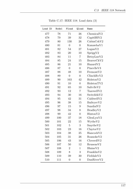
C.3 IEEE 118 Network
Table C.17: IEEE 118: Load data (3)
Load ID Node1 Pload Qload Name
477 78 71 26 ChemicalV2
478 79 39 32 CapitlHlV2
479 80 130 26 CabinCrkV2
480 81 0 0 KanawhaV1
481 82 54 27 LoganV2
482 83 20 10 SpriggV2
483 84 11 7 BetsyLneV2
484 85 24 15 BeaverCkV2
485 86 21 10 HazardV2
486 87 0 0 PinevlleV3
487 88 48 10 FremontV2
488 89 0 0 ClinchRvV2
489 90 163 42 HolstonV2
490 91 10 0 HolstonTV2
491 92 65 10 SaltvlleV2
492 93 12 7 TazewellV2
493 94 30 16 SwitchbkV2
494 95 42 31 CaldwellV2
495 96 38 15 BaileysvV2
496 97 15 9 SundialV2
497 98 34 8 BradleyV2
498 99 42 0 HintonV2
499 100 37 18 GlenLynV2
500 101 22 15 WytheV2
501 102 5 3 SmytheV2
502 103 23 16 ClaytorV2
503 104 38 25 HancockV2
504 105 31 26 RoanokeV2
505 106 43 16 CloverdlV2
506 107 50 12 ReusensV2
507 108 2 1 BlaineV2
508 109 8 3 FranklinV2
509 110 39 30 FieldaleV2
510 111 0 0 DanRiverV2
117

C Network Data
Table C.18: IEEE 118: Generation data (1)
Gen-ID Node1 Pgen Pmax Qmax Pmin Qmin Uset Name
601 1 0 100 15 0 -5 95.50 RiversdeV2
602 4 0 100 300 0 -300 99.80 NwCarlslV2
603 6 0 100 50 0 -13 99 KankakeeV2
604 8 0 100 300 0 -300 101.50 OliveV1
605 10 450 550 200 0 -147 105 BreedV1
606 12 85 185 120 0 -35 99 TwinBrchV2
607 15 0 100 30 0 -10 97 FtWayneV2
608 18 0 100 50 0 -16 97.30 McKinleyV2
609 19 0 100 24 0 -8 96.20 LincolnV2
610 24 0 100 300 0 -300 99.20 TrentonV2
611 25 220 320 140 0 -47 105 TannrsCkV2
612 26 314 414 1000 0 -1000 101.50 TannrsCkV1
613 27 0 100 300 0 -300 96.80 MadisonV2
614 31 7 107 300 0 -300 96.70 DeerCrkV2
615 32 0 100 42 0 -14 96.30 DelawareV2
616 34 0 100 24 0 -8 98.40 RockhillV2
617 36 0 100 24 0 -8 98 SterlingV2
618 40 0 100 300 0 -300 97 WestEndV2
619 42 0 100 300 0 -300 98.50 HowardV2
620 46 19 119 100 0 -100 100.50 WLancstV2
621 49 204 304 210 0 -85 102.50 PhiloV2
622 54 48 148 300 0 -300 95.50 TorreyV2
623 55 0 100 23 0 -8 95.20 WagenhlsV2
624 56 0 100 15 0 -8 95.40 SunnysdeV2
625 59 155 255 180 0 -60 98.50 TiddV2
626 61 160 260 300 0 -100 99.50 WKammerV2
627 62 0 100 20 0 -20 99.80 NatriumV2
628 65 391 491 200 0 -67 100.50 MuskngumV1
629 66 392 492 200 0 -67 105 MuskngumV2
630 70 0 100 32 0 -10 98.40 PortsmthV2
631 72 0 100 100 0 -100 98 HillsbroV2
632 73 0 100 100 0 -100 99.10 SargentsV2
633 74 0 100 9 0 -6 95.80 BellefntV2
634 76 0 100 23 0 -8 94.30 DarrahV2
635 77 0 100 70 0 -20 100.60 TurnerV2
636 80 477 577 280 0 -165 104 CabinCrkV2
637 85 0 100 23 0 -8 98.50 BeaverCkV2
638 87 4 104 1000 0 -100 101.50 PinevlleV3
118

C.3 IEEE 118 Network
Table C.19: IEEE 118: Generation data (2)
Gen-ID Node1 Pgen Pmax Qmax Pmin Qmin Uset Name
639 89 607 707 300 0 -210 100.50 ClinchRvV2
640 90 0 100 300 0 -300 98.50 HolstonV2
641 91 0 100 100 0 -100 98 HolstonTV2
642 92 0 100 9 0 -3 99 SaltvlleV2
643 99 0 100 100 0 -100 101 HintonV2
644 100 252 352 155 0 -50 101.70 GlenLynV2
645 103 40 140 40 0 -15 100.10 ClaytorV2
646 104 0 100 23 0 -8 97.10 HancockV2
647 105 0 100 23 0 -8 96.50 RoanokeV2
648 107 0 100 200 0 -200 95.20 ReusensV2
649 110 0 100 23 0 -8 97.30 FieldaleV2
650 111 36 136 1000 0 -100 98 DanRiverV2
651 112 0 100 1000 0 -100 97.50 DanvilleV2
652 113 0 100 200 0 -100 99.30 DeerCrkV2
653 116 0 100 1000 0 -1000 100.50 KygerCrkV2
999001 10 0 50 15 0 -15 105 Wind1
999002 40 0 50 15 0 -15 97 Wind2
999003 42 0 50 15 0 -15 98.50 Wind3
999004 34 0 50 15 0 -15 98.40 Wind4
999005 55 0 50 15 0 -15 95.20 Wind5
999006 59 0 50 15 0 -15 98.50 Wind6
999007 61 0 50 15 0 -15 99.50 Wind7
999008 112 0 50 15 0 -15 97.50 Wind8
999011 12 0 20 1 0 -1 99 PV1
999012 32 0 20 1 0 -1 96.30 PV2
999013 25 0 20 1 0 -1 105 PV3
999014 70 0 20 1 0 -1 98.40 PV4
999015 62 0 20 1 0 -1 99.80 PV5
999016 65 0 20 1 0 -1 100.50 PV6
999017 90 0 20 1 0 -1 98.50 PV7
119

C Network Data
Table C.20: IEEE 118: Pumped Hydro
ID Sammelschiene Info Name
999021 113 PSK1 PumpedHydro1
999022 19 PSK2 PumpedHydro2
999023 36 PSK3 PumpedHydro3
999024 24 PSK4 PumpedHydro4
999025 62 PSK5 PumpedHydro5
999026 89 PSK6 PumpedHydro6
Table C.21: IEEE 118: Transformer data
Trafo ID Node1 Node2 VLevel1 VLevel2 Sr Sr_max U_k
701 8 5 339.83 138 100 0 2.67
702 26 25 331.20 138 100 0 3.82
703 30 17 331.20 138 100 0 3.88
704 38 37 322.58 138 100 0 3.75
705 63 59 331.20 138 100 0 3.86
706 64 61 339.83 138 100 0 2.68
707 65 66 322.58 138 100 0 3.70
708 68 69 322.58 138 100 0 3.70
709 81 80 322.58 138 100 0 3.70
Table C.22: IEEE 118: Feeder
Feeder ID Node1 Uabs Uphase Name Info
901 69 103.50 30 SpornV2 Feeder
120

C.3 IEEE 118 Network
Table C.23: IEEE 118: Shunt compensation
Shunt ID Node1 Q
801 5 -40
802 17 0
803 34 14
804 37 -25
805 44 10
806 45 10
807 46 10
808 48 15
809 74 12
810 79 20
811 82 20
812 83 10
813 105 20
814 107 6
815 110 6
121

C Network Data
C.4 2 Area Network
Per unit generator data rated on 900 MVA and 20 kV
Xd = 1.8 Xq = 1.7 Xl = 0.2 X′d = 0.3
X′q = 0.55 X
′′d = 0.25 X
′′q = 0.25 Ra = 0.0025
T′d0 = 8s T
′q0 = 0.4s T
′′d0 = 0.03s T
′′q0 = 0.05s
Per unit line parameters rated on 100 MVA and 230 kV
r = 0.0001 pu/km xL = 0.001 pu/km
bC = 0.00175 pu/km
Transformer
Impedance j 0.15 per unit on 900 MVA
Load
Bus7 :
PL = 967 MW QL = 100 MVAr QC = 200 MVAr
Bus9 :
PL = 1767 MW QL = 100 MVAr QC = 350 MVAr
122

C.5 5 Area Network
C.5 5 Area Network
Table C.24: Generation conditions for two loadflow cases
Case 1 Case 6
P Q No. Units P Q No. Units
MW Mvar MW Mvar
HPS1 75.2 77.9 4 0 -102 2
BPS2 600 95.6 6 560 -53 3
EPS2 500 132.7 5 490 -7 3
MPS2 491.7 122.4 6 488 -61 3
VPS2 375 132.8 4 490 3.7 3
LPS3 600 132.8 7 550 9.4 6
YPS3 313.3 51.5 3 393 -6.9 2
CPS4 279 59.3 3 270 4.7 3
GPS4 258.3 54.5 6 245 3.9 3
SPS4 350 52.3 4 380 25.2 2
TPS4 350 128.7 4 350 -32.6 3
NPS5 300 27.3 2 270 -42.2 1
PPS5 109 27.2 4 120 -11.2 2
TPS5 200 40.1 4 200 -9.7 4
Table C.25: Shunt Capacitor and Reactor Banks
Case 1 Case 6
Mvar Mvar
Capacitor
212 400 400
216 300 300
409 60 60
411 30 30
Reactor
414 30 30
415 60 60
416 60 90
123

C Network Data
Table
C.2
6:
Gen
erato
rP
ara
meters
Nam
eN
ode
Ratin
gH
Xa
Xd
Xq
Xd’
Tdo’
Xd”
Tdo”
Xq’
Tqo’
Xq”
Tqo”
MV
AM
Ws/
MV
Apu
pu
pu
pu
spu
spu
spu
sH
PS1
101
333.3
2.9
0.1
41.1
0.6
50.2
58.5
0.2
40.0
50.6
0.4
0.2
50.2
BP
S2
201
666.7
2.6
0.2
1.8
1.7
50.3
8.5
0.2
10.0
40.7
0.3
0.2
10.0
8E
PS2
202
555.6
2.2
0.1
72.2
2.1
0.3
4.5
0.2
0.0
40.5
1.5
0.2
10.0
6M
PS2
204
666.7
2.6
0.2
1.8
1.7
50.3
8.5
0.2
10.0
40.7
0.3
0.2
10.0
8V
PS2
203
555.6
2.1
0.2
2.3
1.7
0.3
50.2
50.0
30.4
20.2
50.2
5L
PS3
301
666.7
2.2
0.2
2.7
1.5
0.3
7.5
0.2
50.0
40.8
50.8
50.2
50.1
2Y
PS3
302
444.4
2.8
0.1
52
1.8
0.2
57.5
0.2
0.0
40.8
50.8
50.2
0.2
5C
PS4
402
333.3
2.4
0.2
1.9
1.8
0.3
6.5
0.2
60.0
35
0.5
51.4
0.2
60.0
4G
PS4
404
333.3
3.2
0.1
82.2
1.4
0.3
29
0.2
40.0
40.7
51.4
0.2
40.1
3SP
S4
403
444.4
2.1
0.2
2.3
1.7
0.3
50.2
50.0
30.4
20.2
50.2
5T
PS4
401
444.4
2.1
0.2
2.3
1.7
0.3
50.2
50.0
30.4
20.2
50.2
5N
PS5
501
333.3
2.8
0.1
52.2
1.7
0.3
7.5
0.2
40.0
25
0.8
1.5
0.2
40.1
TP
S5
502
250
3.2
0.2
21.5
0.3
7.5
0.2
20.0
40.8
30.2
20.2
PP
S5
503
166.7
60.1
52.3
20.2
55
0.1
70.0
22
0.3
51
0.1
70.0
35
124

C.5 5 Area Network
Table C.27: Transformers: R and X in p.u. on 100MVA
Node i Node j Rating Uk in % X R
HPS1 101 102 333.3 12 0.036 0.00018BPS2 201 206 666.7 16 0.024 0.00012EPS2 202 209 555.6 16 0.0288 0.000144VPS2 203 208 555.6 17 0.0306 0.000153MPS2 204 215 666.7 16 0.024 0.00012LPS3 301 303 666.7 16 0.024 0.00012YPS3 302 312 444.4 15 0.0338 0.000169TPS4 401 410 444.4 15 0.0338 0.000169CPS4 402 408 333.3 17 0.051 0.000255SPS4 403 407 444.4 15 0.0338 0.000169GPS4 404 405 333.3 17 0.051 0.000255NPS5 501 504 333.3 17 0.051 0.000255TPS5 502 505 250 16 0.064 0.00032PPS5 503 506 166.7 16 0.1 0.0005
209 210 625 17 0.0272 0.000136213 214 625 17 0.0272 0.000136304 313 500 16 0.032 0.00016305 311 500 12 0.024 0.00012305 314 700 17 0.0243 0.0001215308 315 370 10 0.027 0.000135413 414 750 6 0.008 0.00004
Table C.28: SVC Data
Node Case 1 Case 6
Mvar Mvar205 -68.3 -29.4313 71.4 54.2412 58.2 0507 22.6 -3.7509 10.6 -109.3
125

C Network Data
Table C.29: Line data in p.u. on 100MVA
Node i Node j R X b
102 217 0.0042 0.0334 1.634102 217 0.0039 0.031 1.52102 309 0.0023 0.0178 0.874102 309 0.0109 0.0868 0.76205 206 0.0048 0.038 1.862205 416 0.0019 0.023 1.46206 207 0.0023 0.0178 0.874206 212 0.0033 0.0264 1.292206 215 0.0033 0.0264 1.292207 208 0.0009 0.007 0.342207 209 0.0008 0.0062 0.076208 211 0.001 0.0083 0.912209 212 0.0045 0.0356 0.437210 213 0.0005 0.0073 3.08211 212 0.0007 0.0054 0.266211 214 0.0019 0.0155 0.19212 217 0.007 0.0558 0.684214 216 0.001 0.0077 0.095214 217 0.0049 0.0388 0.475215 216 0.0026 0.0202 0.988215 217 0.0036 0.0287 1.406216 217 0.0051 0.0403 0.494303 304 0.001 0.014 1.48303 305 0.0006 0.008 3.4304 305 0.0003 0.004 0.424305 306 0.0002 0.003 0.32305 307 0.0002 0.0023 0.894306 307 0.0001 0.0012 0.127307 308 0.0012 0.0163 6.89309 310 0.0045 0.0357 1.748310 311 0 -0.0169 0312 313 0.002 0.015 0.9313 314 0.0005 0.005 0.52315 509 0.0035 0.025 0.38405 406 0.002 0.0238 0.762405 408 0.0054 0.05 0.189405 409 0.006 0.0407 2.37406 407 0.0003 0.0038 0.124407 408 0.0042 0.0513 0.412
126

C.5 5 Area Network
Table C.30: Line data in p.u. on 100MVA
Node i Node j R X b
408 410 0.0055 0.064 2.02409 411 0.0052 0.0355 0.92410 411 0.0043 0.0532 0.427410 412 0.0011 0.0133 1.708410 413 0.002 0.0247 0.8411 412 0.0006 0.0076 0.244414 415 0.001 0.0125 0.78415 416 0.0019 0.023 1.46504 507 0.0115 0.075 1.12504 508 0.013 0.0095 1.74505 507 0.0008 0.0085 0.06505 508 0.0025 0.028 0.17506 507 0.0008 0.0085 0.06506 508 0.003 0.028 0.14507 508 0.002 0.019 0.09507 509 0.015 0.11 1.8
127
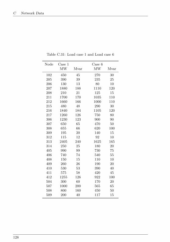
C Network Data
Table C.31: Load case 1 and Load case 6
Node Case 1 Case 6MW Mvar MW Mvar
102 450 45 270 30205 390 39 235 25206 130 13 80 10207 1880 188 1110 120208 210 21 125 15211 1700 170 1035 110212 1660 166 1000 110215 480 48 290 30216 1840 184 1105 120217 1260 126 750 80306 1230 123 900 90307 650 65 470 50308 655 66 620 100309 195 20 140 15312 115 12 92 10313 2405 240 1625 165314 250 25 180 20405 990 99 730 75406 740 74 540 55408 150 15 110 10409 260 26 190 20410 530 53 390 40411 575 58 420 45412 1255 126 922 100504 300 60 170 20507 1000 200 565 65508 800 160 450 50509 200 40 117 15
128

Bibliography
[1] K. Baker, G. Hug, and Xin Li. Inclusion of inter-temporal constraints into a
distributed newton-raphson method. In North American Power Symposium
(NAPS), 2012, pages 1–6. IEEE, 2012.
[2] K. Baker, G. Hug, and Xin Li. Optimal integration of intermittent energy
sources using distributed multi-step optimization. In Power and Energy Society
General Meeting, 2012 IEEE, pages 1–8, 2012.
[3] H. Behbehani, Z. Lubosny, and J.W. Bialek. Survey of supervisory power
system stabilizers for enhancement of power system stability. In Universities
Power Engineering Conference, 2007. UPEC 2007. 42nd International, pages
426–437, 2007.
[4] P.N. Biskas and A.G. Bakirtzis. Decentralised opf of large multiarea power
systems. Generation, Transmission and Distribution, IEE Proceedings-,
153(1):99–105, Jan 2006.
[5] F. Borelli, A. Bemporad, and M. Morari. Predictive Control for linear and
hybrid systems. ETH, 2011.
[6] C. Breuer, D. Echternacht, C. Linnemann, and A. Moser. Technical and
economic comparison of national and joint cross-border curative congestion
management application. In Energy Market (EEM), 2011 8th International
Conference on the European, pages 33–38, May 2011.
[7] P. Brogan. The stability of multiple, high power, active front end voltage
sourced converters when connected to wind farm collector systems. In EPE
Wind 2010, 2010.
[8] T. Demiray. Simulation of Power System Dynamics using Dynamic Phasor
Models. PhD thesis, ETH Zurich, 2008.
[9] Online Documentation. PSS/E 25. Siemens, December 1997.
[10] K. Dong-Joon, M. Young-Hwan, and N. Hae-Kon. A practical approach to hvdc
system control for damping subsynchronous oscillation using the novel eigen-
value analysis program. Power Systems, IEEE Transactions on, 22(4):1926–
1934, Nov 2007.
129
C BIBLIOGRAPHY
[11] K. Dong-Joon, M. Young-Hwan, and N. Hae-Kon. Ssr small-signal stability
analysis program of power systems and its application to ieee benchmark sys-
tems. In Power Tech, 2007 IEEE Lausanne, pages 161–166, July 2007.
[12] D. Dotta, A.S. Silva, and I.C. Decker. Wide-area measurements-based two-
level control design considering signal transmission delay. IEEE Transactions
on Power Systems, 24(1):208–216, 2009.
[13] Haesen E. Multi-Objective Optimization of the Integration of Stochastic Dis-
tributed Energy Resources in Electricity Grids. PhD thesis, Univerity Leuven,
2009.
[14] Entso-E. Operation handbook. Technical report, Entso-E, 2004.
[15] O. Follinger. Regelungstechnik. huthig. Technical report, ISBN 3–7785–2336–
8, 1994.
[16] P. Fortenbacher. Power flow modeling and grid constraint handling in power
grids with high res in-feed, controllable loads, and storage devices. Master’s
thesis, KIT and ETH, 2011.
[17] Yong Fu, M. Shahidehpour, and Zuyi Li. Security-constrained unit commit-
ment with ac constraints*. Power Systems, IEEE Transactions on, 20(3):1538–
1550, 2005.
[18] A. Fuchs, M. Imhof, T. Demiray, and M. Morari. Stabilization of large power
systems using vsc–HVDC and model predictive control. IEEE Transactions
on Power Delivery, 29(1):480–488, 2014.
[19] O. Galland. The short-run security-contrained economic dispatch. Master’s
thesis, KTH Stockholm, 2012.
[20] M. Gibbard and D. Vowles. Simplified 14-
Generator Model of the SE Australian Power System.
http://www.eleceng.adelaide.edu.au/groups/PCON/PowerSystems, 2007.
[21] M. Gibbard, D. Vowles, and P. Pourbeik. Interactions between, and effective-
ness of, power system stabilizers and facts device stabilizers in multimachine
systems. Power Systems, IEEE Transactions on, 15(2):748–755, 2000.
[22] M.J. Gibbard. Co-ordinated design of multimachine power system stabilisers
based on damping torque concepts. Generation, Transmission and Distribution,
IEE Proceedings C, 135(4):276–284, Jul 1988.
[23] M. Glavic and T. Van Cutsem. Investigating state reconstruction from scarce
synchronized phasor measurements. In IEEE PowerTech, Trondheim, 2005.
130

BIBLIOGRAPHY
[24] S. Gomes, N. Martins, and C. Portela. Modal analysis applied to s-domain
models of ac networks. In Power Engineering Society Winter Meeting, 2001.
IEEE, volume 3, pages 1305 –1310 vol.3, 2001.
[25] S. Gomes, N. Martins, and C. Portela. Sequential computation of transfer
function dominant poles of s-domain system models. Power Systems, IEEE
Transactions on, 24(2):776–784, May 2009.
[26] S. Gomes, N. Martins, and A. Stankovic. Improved controller design using
new dynamic phasor models of svc’s suitable for high frequency analysis. In
Transmission and Distribution Conference and Exhibition, 2005/2006 IEEE
PES, pages 1436–1444, 2006.
[27] G. Gross, C.F. Imparato, and P.M. Look. A tool for the comprehensive anal-
ysis of power system dynamic stability. Power Apparatus and Systems, IEEE
Transactions on, PAS-101(1):226–234, Jan 1982.
[28] R. M. Hamouda, M.R. Iravani, and R. Hackam. Torsional oscillations of series
capacitor compensated ac/dc systems. Power Systems, IEEE Transactions on,
4(3):889–896, Aug 1989.
[29] L. Harnefors. Analysis of subsynchronous torsional interaction with power
electronic converters. Power Systems, IEEE Transactions on, 22(1):305–313,
Feb 2007.
[30] K. Heussen, S. Koch, A. Ulbig, and G. Andersson. Unified system-level mod-
eling of intermittent renewable energy sources and energy storage for power
system operation. Systems Journal, IEEE, 6(1):140–151, 2012.
[31] G. Hirsch. Semianalytische Simulation von systemimmanenten elektro-
mechanischen Pendelschwingungen in Verbundnetzen. PhD thesis, Universitat
der Bundeswehr Hamburg, 2003.
[32] G. Hirsch. Undamped inherent inter-area oscillations in power grids. Electrical
Engineering, 88(4):259–273, 2006.
[33] G. Hug-Glanzmann and G. Andersson. N-1 security in optimal power flow
control applied to limited areas. Generation, Transmission Distribution, IET,
3(2):206–215, 2009.
[34] IEEE. Standard for Calculating the Current-Temperature of Bare Overhead
Conductors. IEEE Std 738-2006 (Revision of IEEE Std 738-1993), 1:c1–59,
2007.
131
C BIBLIOGRAPHY
[35] M.R. Iravani, A.K.S. Chandhary, W.J. Giesbrecht, I.E. Hassan, A.J.F. Keri,
K.C. Lee, J.A. Martinez, A.S. Morched, B.A. Mork, M. Parniani, A. Sarshar,
D. Shirmohammadi, R.A. Walling, and D.A. Woodford. Modelling and analysis
guidelines for slow transients. ii. controller interactions; harmonic interactions.
Power Delivery, IEEE Transactions on, 11(3):1672–1677, Jul 1996.
[36] E. Johansson. Detailed description of Synchronous Machine Models used in
Simpow. ABB, December 2001.
[37] D. Jovcic, N. Pahalawaththa, M. Zavahir, and H.A. Hassan. Svc dynamic
analytical model. Power Delivery, IEEE Transactions on, 18(4):1455–1461,
2003.
[38] I. Kamwa, R. Grondin, and Y. Hebert. Wide-area measurement based sta-
bilizing control of large power systems-a decentralized/hierarchical approach.
IEEE Transactions on Power Systems, 16(1):136–153, 2001.
[39] R. Kankanamalage and G. Hug-Glanzmann. Usage of storage for optimal
exploitation of transfer capacity: A predictive control approach. In Power and
Energy Society General Meeting, 2011 IEEE, pages 1–8, 2011.
[40] S. Kapoor and PM. Vaidya. Fast algorithms for convex quadratic programming
and multicommodity flows. Proceedings 18th Annual ACM Symposium on
Tjheroy of Computing, 1:147 – 159, 1986.
[41] C. Karawita and U.D. Annakkage. Multi-infeed hvdc interaction studies us-
ing small-signal stability assessment. Power Delivery, IEEE Transactions on,
24(2):910–918, April 2009.
[42] C. Karawita and U.D. Annakkage. A hybrid network model for small signal
stability analysis of power systems. Power Systems, IEEE Transactions on,
25(1):443–451, Feb 2010.
[43] B.H. Kim and R. Baldick. A comparison of distributed optimal power flow
algorithms. Power Systems, IEEE Transactions on, 15(2):599–604, May 2000.
[44] H. Kocewiak, J. Hjerrild, and C.L. Bak. Wind turbine converter control inter-
action with complex wind farm systems. Renewable Power Generation, IET,
7(4):380–389, July 2013.
[45] Y. Kokai, C. Fukui, and T. Kawahara. Power systems stability solutions for a
low-carbon society. In Hitachi Review Vol. 60, No. 3, 2011.
[46] P. Krause. Analysis of electric machinery and drive systems. IEEE Press,
2002.
132

BIBLIOGRAPHY
[47] E.S. Kuh and R.A. Rohrer. The state-variable approach to network analysis.
Proceedings of the IEEE, 53(7):672–686, July 1965.
[48] A. Kumar, S.C. Srivastava, and S.N. Singh. Congestion management in compet-
itive power market: A bibliographical survey. Electric Power Systems Research,
76(13):153 – 164, 2005.
[49] P. Kundur. Power system stability and control. McGraw, 1994.
[50] P. Kundur, G.J. Rogers, D.Y. Wong, L. Wang, and M.G. Lauby. A compre-
hensive computer program package for small signal stability analysis of power
systems. Power Systems, IEEE Transactions on, 5(4):1076 –1083, nov 1990.
[51] F. Kunz and A. Zerrahn. The benefit of coordinating congestion management
in germany. In DIW Berlin - German Institute for Economic Research, 2013.
[52] Yong Li, C. Rehtanz, S. Ruberg, Longfu Luo, and Yijia Cao. Wide-area robust
coordination approach of HVDC and facts controllers for damping multiple
interarea oscillations. IEEE Transactions on Power Delivery, 27(3):1096–1105,
2012.
[53] L. Lima, N. Martins, and S. Carneiro Jr. Augmented state-space formulations
for the study of electric network including distributed-parameter transmission
line models. In International Conference on Power Systems Transients, 1999.
[54] M. Liserre, R. Teodorescu, and F. Blaabjerg. Stability of photovoltaic and
wind turbine grid-connected inverters for a large set of grid impedance values.
Power Electronics, IEEE Transactions on, 21(1):263–272, Jan 2006.
[55] J. Lofberg. Yalmip : a toolbox for modeling and optimization in matlab. In
Computer Aided Control Systems Design, 2004 IEEE International Symposium
on, pages 284–289, 2004.
[56] O. Lotter. Natural minimal set of state equations of linear power grid. Electrical
Engineering, Springer, 5:405–409, 2007.
[57] J. Maciejowski. Predictive control: with constraints. Pearson education, 2002.
[58] B. Marinescu, J-M Coulondre, P. Tsamasphyrou, and J.-Y. Bourmaud. Im-
proving tso’s coordination for cross-border redispatch: a discussion of possible
approaches in the european context. In CIGRE/IEEE PES, 2005. Interna-
tional Symposium, pages 378–385, Oct 2005.
[59] Hui Ni, G.T. Heydt, and L. Mili. Power system stability agents using robust
wide area control. IEEE Transactions on Power Systems, 17(4):1123–1131,
2002.
133

C BIBLIOGRAPHY
[60] G. Oggioni, Y. Smeers, E. Allevi, and S. Schaible. A generalized nash equilib-
rium model of market coupling in the european power system. Networks and
Spatial Economics, 12(4):503–560, 2012.
[61] F. Okou, L.-A. Dessaint, and O. Akhrif. Power systems stability enhancement
using a wide-area signals based hierarchical controller. IEEE Transactions on
Power Systems, 20(3):1465–1477, 2005.
[62] B. Pal and B. Chaudhuri. Robust Control in Power Systems. Springer, 2005.
[63] M. Parniani and M.R. Iravani. Computer analysis of small-signal stability of
power systems including network dynamics. Generation, Transmission and
Distribution, IEE Proceedings-, 142(6):613–617, Nov 1995.
[64] R.A. Ramos, L.F.C. Alberto, and N.G. Bretas. A new methodology for the
coordinated design of robust decentralized power system damping controllers.
IEEE Transactions on Power Systems, 19(1):444–454, 2004.
[65] J. Rawlings and D. Mayne. Model predictive Control: Theory and design. Nob
Hill Publishing, 2009.
[66] M.G. Safonov and R.Y. Chiang. A schur method for balanced-truncation model
reduction. IEEE Transactions on Automatic Control, 34(7):729–733, 1989.
[67] O. Samuelsson, H. Johannsdottir, N. Gustavsson, T. Hrafnsson, D. Karlsson,
D. Novosel, J. Salj, and A. Sollie. Power system damping in iceland based
on phasor measurements. In Power Systems and Communication Systems
Infrastructures for the Future, Beijing, China, 2002.
[68] D. Shirmohammadi, B. Wollenberg, A. Vojdani, P. Sandrin, M. Pereira,
F. Rahimi, T. Schneider, and B. Stott. Transmission dispatch and conges-
tion management in the emerging energy market structures. Power Systems,
IEEE Transactions on, 13(4):1466–1474, Nov 1998.
[69] J.G. Slootweg, J. Perssonand, A.M. van Voordenand, G.C. Paapand, and W.L.
Kling. A study of the eigenvalue analysis capabilities of power system dynamics
simulation software. In 14th Power Systems Computation Conference Sevilla
Spain, 2002.
[70] A. Ulbig and G. Andersson. On operational flexibility in power systems. In
Power and Energy Society General Meeting, 2012 IEEE, pages 1–8, 2012.
[71] A. Ulbig, S. Koch, and G. Andersson. The power nodes modeling framework
modeling and assessing the operational flexibility of hydro power units. In XII
SEPOPE,Rio de Janeiro, Brazil, 2012.
134

BIBLIOGRAPHY
[72] S.L. Varricchio, S. Gomes, and N. Martins. s-domain approach to reduce
harmonic voltage distortions using sensitivity analysis. In Power Engineering
Society Winter Meeting, 2001. IEEE, volume 2, pages 809–814 vol.2, 2001.
[73] A. Venkat. Distributed Model Predictive Control: Theory and Application. PhD
thesis, University of Wisconsin-Madison, 2006.
[74] A.N. Venkat, I.A. Hiskens, J.B. Rawlings, and S.J. Wright. Distributed MPC
strategies with application to power system automatic generation control.
IEEE Transactions on Control Systems Technology, 16(6):1192–1206, 2008.
[75] D.J. Vowles and M.J. Gibbard. Mudpack - a software package for the analysis
of the small-signal dynamic performance and control of large electric power
systems. School of Electrical & Electronic Engineering, The University of
Adelaide, South Australia, 12 2007.
[76] D.J. Vowles and M.J. Gibbard. Power systems dynamics group contribution
to the ieee benchmark systems for stability controls task force, 2014.
[77] LZ Yao, G Strbac, XP Zhang, R Allan, M Bradley, HB Wan, and P Turner.
A concurrent optimal power flow for enforcement of system solvability, voltage
and thermal constraints. 13th PSCC, Trondheim, Norway, 1:351–357, 1999.
[78] R. Zarate-Mihano, A.J. Conejo, and F. Milano. Opf-based security redis-
patching including facts devices. Generation, Transmission Distribution, IET,
2(6):821–833, November 2008.
[79] Lidong Zhang, L. Harnefors, and H-P. Nee. Modeling and control of vsc-hvdc
links connected to island systems. Power Systems, IEEE Transactions on,
26(2):783–793, May 2011.
135

136

Author’s Publications
[80] M. Kahl, C. Freye, and T. Leibfried. A cooperative multi-area optimization
with renewable generation and storage devices. Power Systems, IEEE Trans-
actions on, 2014. (Accepted for future publication).
[81] M. Kahl and T. Leibfried. Modellbasierte Regelungsalgorithmen fur das En-
ergienetz der Zukunft. In Lecture Notes in Informatics (LNI) Berlin, 2011.
[82] M. Kahl and T. Leibfried. Decentralized model predictive control of electrical
power systems. In International Conference on Power Systems Transients
(IPST2013) Vancouver, 2013.
[83] M. Kahl, D. Uber, and T. Leibfried. Dynamic state estimator for voltage
stability and low frequency oscillation detection. In IEEE Innovative Smart
Grid Technologies Conference- Asia, 2014.
[84] M. Kahl, S. Wenig, and T. Leibfried. Dezentrale modellpradiktive Opti-
mierungsstrategien zur Einbindung erneuerbarer Erzeugungskapazitat und Spe-
ichersysteme. In Konferenz fur Nachhaltige Energieversorgung und Integration
von Speichern-NEIS Hamburg, 2013.
[85] U. Reiner, M. Kahl, T. Leibfried, F. Allerding, and H. Schmeck. Meregiomobil-
labor - entwicklungsumgebung fur zukunftige smart-homes. In ETG Kongress
Leipzig, 2010.
137

138
Supervised Theses
[86] A. Benazza. Verfahren zur Modellierung von Energieubertragungsnetzen. Stu-
dienarbeit, KIT, 2010.
[87] M. Bergner. Modellierung einer Synchronmaschine und deren Interaktion mit
einem dynamischen Netzmodell. Studienarbeit, KIT, 2012.
[88] W. Biener. Synthese von dezentralen Zustandsreglern mittels linearer Matrix-
gleichungen fur Elektroenergiesysteme. Studienarbeit, KIT, 2012.
[89] J. Chang. Dezentrale Regelung eines Netzverbundes. Masterarbeit, KIT, 2014.
[90] A. Engelmann. Zustandsschatzung fur transiente Betriebsfalle in einem En-
ergieubertragungsnetz. Bachelorarbeit, KIT, 2013.
[91] E. Fastanz. Simulation von Pendelschwingungen im Verbundnetz. Studienar-
beit, KIT, 2014.
[92] C. Freye. Verfahren zur Modellbasierte Betriebsfuhrung eines BHKWs. Bach-
elorarbeit, KIT, 2010.
[93] C. Freye. Kooperationsbasierte modellpradiktive Optimierung von Elektroen-
ergiesystemen unter Berucksichtigung von Netzrestriktionen. Masterarbeit,
KIT, 2013.
[94] F. Gotz. Auslegung von Power Systems Stabilisern mittels Modal-Analyse von
Energieubertragungsnetzen. Bachelorarbeit, KIT, 2010.
[95] S. Knauff. Implementierung einer Modellpradiktiven Regelung in DigSilent
PowerFactory. Bachelorarbeit, KIT, 2013.
[96] M. Lang. Modellierung von Selbstgefuhrten Stromrichtern. Bachelorarbeit,
KIT, 2011.
[97] S. Loffler. Automatisierte Leistungsdatenerfassung in einem Smart-home.
Bachelorarbeit, KIT, 2011.
[98] M. Ling. Entwicklung eines generischen Modells fur netzgefuhrte Stromrichter.
Technical report, KIT, 2010.
139

C SUPERVISED THESES
[99] T. Lommel. Erweiterte optimale Einbindung von konventionellen und dezen-
tralen Kraftwerken unter Berucksichtigung von Netzrestriktionen. Diplomar-
beit, KIT, 2012.
[100] L. Merkert. Modellpradiktive Regelung eines Energieubertragungsnetzes.
Diplomarbeit, KIT, 2011.
[101] N. Meyer-Hubner. Modellierung von stromrichterbetriebenen Anlagen und
deren Regelung in einem realen Verteilnetz. Studienarbeit, KIT, 2012.
[102] P. Muller. Beschreibung von unsymmetrischen Netzzustanden mittels eines
dynamischen Modells. Studienarbeit, KIT, 2012.
[103] J. Noteisen. Modellierung und Regelung eines TCSC im Verbundnetz. Bach-
elorarbeit, KIT, 2012.
[104] S. Schneider. Optimale Einbindung von konventionellen und dezentralen
Kraftwerken unter Berucksichtigung von Netzrestriktionen. Bachelorarbeit,
KIT, 2011.
[105] T. Strobel. Entwicklung eines generischen Windkraftanlagen Modells. Bach-
elorarbeit, KIT, 2011.
[106] A. Trumpf. Auslegung von Power System Stabilisern mittels Eigenwertanal-
yse. Bachelorarbeit, KIT, 2013.
[107] D. Uber. Entwicklung eines Zustandschatzers fur dynamische Betrieb-
szustande von Elektroenergiesystemen. Diplomarbeit, KIT, 2012.
[108] A. Wober. Stabilitatsuntersuchungen von stromrichtergespeisten Anlagen im
Verteilnetz. Bachelorarbeit, KIT, 2012.
[109] C. Wegner. Hierarchische Regelung von Energieubertragungsnetzen im Zus-
tandsraum. Diplomarbeit, KIT, 2011.
[110] S. Wenig. Dezentrale modellpradiktive Optimierungsstrategien zur Ein-
bindung erneuerbarer Erzeugungskapazitaten und Speichersysteme. Diplomar-
beit, KIT, 2013.
140