Cooks River Survey

September 2005

Prepared for the Environmental Services of the Marrickville Council by A/Prof. A.D.Albani – School of Biological, Earth and Environmental Sciences, University of NewSouth Wales. Additional research material by G. Kollias.

2

Content

Introduction…………………………………………. 3

Methodology………………………………….…….. 4

Sampling……………………………………..……… 5

Laboratory procedures……………………………….. 7

Results…………………………………….………… 8

Sediment………………………………… 8

Sediment Geochemistry…………………14

Benthic ecology……..…………………. 29

Conclusions………………….……….……..……… 34

References………………………….……..…..……. 35

Appendix 1…………………………….…….…..… 39

Appendix 2……………………………..…………. 41

Appendix 3…………………………………..……. 42

Appendix 4……………………………………..…. 44

Appendix 5………………………………….……. 45

3

Introduction

In October 2002 a survey of Cooks River was conducted by A.D. Albani and members of

the Environmental Services of the Marrickville Council. The samples were analysed for

sediment characteristics, sediment geochemistry and distribution of benthic fauna

(foraminifera, protozoa).

In 2004 additional sampling and further analitycal work (sediment distribution and

geochemistry) was carried out by George Kollias (2004) for his Honours project. This

report is a combination of both studies

The purposes was to determine the nature of the river sediments, their geochemical

characters and the distribution of benthic fauna if present.

Along the Australian coast the environmental pressures due to increased urbanisation and

industrialisation have been addressed by developing a number of Plan of Managements.

One of the difficulties is to establish the level of environmental stress in inlets and

estuaries because of the lack of reference base levels and suitable methodology for the

treatment of long term data. Any attempt to evaluate physio-chemical parameters of the

water masses is, by the very nature of the measurement methodology, time related; it

gives only a snapshot of the environment.

A permanent record of these events is, however, available in the seabed; the distributions

of benthic organisms and sediment characteristics, as well as their geochemistry, reflect

very closely the behaviour and quality of the water masses. The effects of quality

changes, even slight but persistent in time, have a cumulative effects on the seabed.

Cooks River is located 20 km southwest of Sydney CBD, 151°09'E 33°58'S and flows for

23 km from its source in Bankstown to Botany Bay at its northwest shore close to

Sydney’s Kingsford-Smith Airport. The catchment, 98 km2, is extensively developed and

it is home to over 400 000 people, 130 000 dwellings and 100 000 commercial and

industrial premises. Anthropogenic impacts are evident at many locations along the

River, which suffers from relatively poor water quality. The impacts are mainly due to

urban runoff, some dumping of household and trade waste, sewage overflows, industrial

discharges, and littering.

4

Methodology

An integrated methodology has been developed and it has been applied with success in

numerous locations both in Australia and overseas. Such methodology considers three

main variables: sediments characteristics, sediment geochemistry and benthic ecology

based on the disribution of foraminifera (protozoans).

a - Sediments.

Detailed sedimentological investigations have been used to recognise sedimentary

provinces; in addition, sediment data can also be used to estimate the rate of siltation and

provenance of the sediment, and to give an indication of the energy levels affecting the

seabed. Traditionally the approach has been to evaluate the sediment characteristics based

on summarising the size distributions using statistical parameters only; the methodology

here adopted in evaluating the laboratory data is based on a complex statistical analysis

using the totality of the data. This has been found to reveal a number of details much

greater than by the traditional method and to obtain a more comprehensive understanding

of the sedimentary environment (Albani, 1974; Albani et al., 1976, 1991a, 1998).

b – Sediment geochemistry

The sediment geochemistry was based on a standard set of 33 elements. Many of these

are suspected to be toxic to life forms and are likely to be introduced into the area by

human activities. Using these data, geochemical provinces are delineated and an

assessment of potential source of specific elements obtained.

While most of the determinations are carried out on a selected portion of the sediment,

mainly the fine fraction, the technique here adopted examines the totality of the sample

including the interstitial water present in the sediment at the time of the collection. This

approach allows for an underdstanding of the amounts of the heavy metals, which may be

affecting the benthic fauna (Rickwood, 1983; Rickwood et al., 1983, 1992; Albani et al.,

1989b;. 1995).

c- Benthic foraminifera.

Foraminifera are marine unicellular protozoa, which secrete a shell (test) of calcium

carbonate; their size generally ranges from 0.1 to 2 mm. They are very sensitive to

variations in the physico-chemical characteristics of their environment such as salinity,

5

temperature, food availability and water depth. The high abundance of individuals

(population) and the considerable variety of species (assemblage) present in a small

sample of the bottom sediment, even in a restricted environment, make it possible to

recognise any slight changes in the total assemblage, as well as in the various populations.

Often the differences are not in the presence or absence of various species, ie. at the

assemblage level, but in the relative abundance of the various species.

Because of their short life span and the fact that they secrete a shell, the occurrence of

foraminifera is not restricted to the time of the sampling and it offers a time-integrated

view of the water qualities (Albani, 1968, 1978, 1979, 1993; Albani, et al., 1984, 1991b,

1998, 2001; Johnson and Albani, 1973; Serandrei Barbero et al., 1989). All the

individuals are identified through microscopic examination, their number recorded and,

finally, expressed as percentage species population of the total assemblage present in the

sample and these values form the numerical basis for the statistical analysis.

Sampling

Figure 1 – Locality map and sampling sites

6

In the 2002 sampling program 14 stations (CR1-CR14) (Fig. 1; Table 1) were

selected from the centre of the river at relatively even interval from Sutton Park (Old

Sugar Mill) (sample CR1) to off the Kogarah Golf Club (sample CR12) with additional

samples from Muddy Creek (sample CR13) and close to the river mouth.

The 2004 sampling (samples CR04A-CR15A) were focused towards stormwater inputs

along the river. Note the identifiers of the various stations in maps and diagrams may not

contain the prefix CR for semplicity of representation.

Table 1 – Sediment sample site notes (2002)Sample Site Depth (m)

CR1 Opposite harbour entrance near old sugar mill, Canterbury 1.3?

CR2 Bend in river just DS from end of Younger Av 1.8?

CR3 50m upstream from Wardell Rd bridge 2.8

CR4 50m upstream from footbridge opposite Marrickville Golf Club building 2.6

CR5 50m downstream from Illawarra Rd bridge - downstream from SW drain net withboom net

1.8

CR6 Opposite beach at Warren Park, downstream from Malakoff Tunnel outlet 2.2

CR7 50m downstream from Western Channel trash rack at Mackey Park 2.3

CR8 Half way between Eastern Channel and railway bridge at Tempe 2.2

CR9 100m downstream of Tempe Railway bridge 3.5

CR10 Middle of boat harbour at Tempe 1.9

CR11 Opposite Clubhouse opposite Tempe Reserve 0.7?

CR12 downstream from bridge opposite Kogarah Golf Clubhouse 1.7

CR13 Inside boat harbour inlet just upstream from Mutch Av boat ramp 2.2

CR14 Boat anchorage 200m upstream from last road bridge before mouth 4

Collected 24/10/02 - Note taker - John Lavarack, Marrickville Council

CR15A Stormwater outlet 300m from flour mill 1.3CR14A Opposite McInnes Reserve - Drain between falling banks 2.22CR13A Ecosol unit - 4m from drain 1.8CR12A Steel Park SWO - 4.5m from outlet 1.4CR11A Mackey Park GPT - 3.0m from GPT 0.95CR10A Tempe station - 6.0m from drain 2.3CR09A Wolli Creek - 10m downstream from bridge 3.5CR08A Tempe boat club - 25m from Princess Hwy 1.5CR07A Nth Arncliffe drain - 20m from drain 1.9CR06A Alexandra Canal - 10 m downstream of bridge 2CR05A Muddy Creek - 20m from bridge 1.1CR04A River Mouth - 10m off southern rock wall >5.00

Collected 17/05/04

Sediment from the seabed was obtained using a small dredge (grab) operated from a small

boat and the sample was normally taken from the top 10 cm of surface material; two

bottom samples from the same station locality were obtained: one for the geochemical

study and the other for the sedimentological and ecological study.

7

Laboratory procedures

a- Sedimentology

A 500 gr aliquot is homogenised and a subportion of 50 - 60 gr is wet sieved through a

150µm nylon mesh to separate sand from silt and clay. The sand fraction is then

processed using sieves at 1/4 Φ (phi) (Φ = -log mm/log 2), and the silt/clay fraction

analysed using a Malvern Mastersizer. The percentage values of each fraction is

calculated and these data form the basis for the various numerical correlations.

b- Geochemistry

About 1 kg of sample is dried at 105˚C prior to thorough mixing and subdividing. An

aliquot of about 500 gr is grounded in a tungsten carbide ring mill to ensure particles are

<50 µ in diameter and the resultant powder is remixed and analysed by X-ray

fluorescence spectrometry. In case of trace elements, 4-5 gr aliquots are taken from the

dried, crushed sample and are pressed in a hydraulic ram to produce firm pellets suitable

for XRF analyses. For major elements further aliquots of dried, crushed powder are

ignited in a furnace at 900˚C, pre- and post-weighing enabling determination of 'Loss on

ignition'. Subsequent fusion of the ignited powder with lithium tetraborate is undertaken

according to well established procedures and the resultant melts are cast as glass discs

used for the analyses.

c- Benthic Foraminifera

About 60 cm3 of sample is taken from the original sample and wet sieved through a 63µm

nylon mesh to eliminate silt and clay. The residue is dried and the foraminifera

concentrated using a floatation method (CCl4). All the individuals are identified through

microscopic examination, their number recorded and, finally, expressed as percentage

species population of the total assemblage present in the sample. The percentage

population of each species, with respect to the total assemblage, is calculated and these

values form the numerical basis for the statistical analysis.

d- Numerical treatment of the data

The three data sets are processed using a number of statistical approaches, among which

factor and cluster analyses. The results are plotted on thematic maps to indicate the

8

distributions of the sedimentary and the geochemical provinces and the foraminiferal

biotopes.

These maps reflect the conditions of the sea-bed at the time of sampling and when

compared with the results from similar future studies will reveal time-related changes

(environmental improvements or/and deteriorations) which form the basis for long term

monitoring programs.

Results

Sediment.

Water flow and its energy are the major determinants of sediment erosion, transport, and

deposition in a fluvial/estuarine system such as the Cooks River. The unconsolidated

substrate reflects therefore the relative strength of the energy present; thus grain size is a

function of energy regimes of the water masses and its degree of sorting describes the

persistence of this energy condition. Coarser materials are found in high-energy

environments and finer materials in low-energy environments, with a mixture of both in

areas of fluctuating flow conditions.

The size of the most common occurring particle (mode) represents the particle-sizes that

are best transported and deposited hence it characterize the predominant transport energy.

The unconsolidated sediments present on the seabed of the Cooks River consists primarily

of fine silt with some clay and it represents the product of natural surface run-off from the

catchments. Towards Botany Bay, however, well sorted sand predominates reflecting the

higher energy conditions of the bay environment.

However, superimposed to the fine fraction, a number of medium to coarse sand sediment

populations are noted in many samples. These represent coarse sediments that can be

considered as the product of increased surface run-off possibly due to localised human-

induced processes.

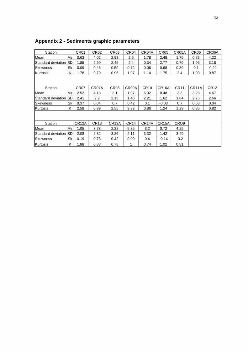
In Appendix 1 the total sediment data set is presented with the grainsize shown as

millimetres as well as phi values. In Appendix 2 the grain size parameters are presented.

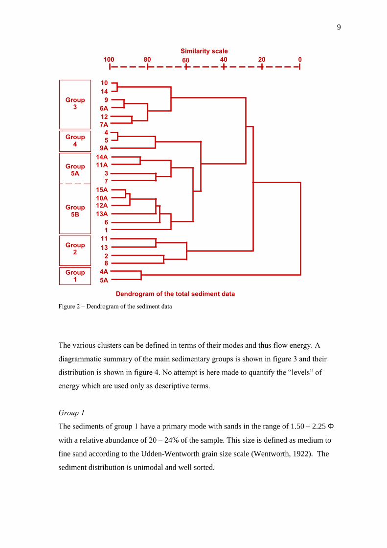
To determine the level of similarity between samples cluster analysis has been applied to

the total data set using the Euclidean distance coefficient to generate the similarity matrix

graphically shown as a dendrogram (Fig. 2).

9

1014

96A127A

45

9A14A11A

37

15A10A12A13A

61

1113

28

4A5A

100 80 60 40 20 0Similarity scale

Group3

Group4

Group5A

Group2

Group1

Group5B

Dendrogram of the total sediment data

Figure 2 – Dendrogram of the sediment data

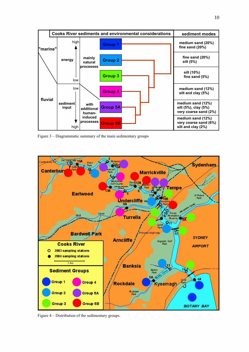
The various clusters can be defined in terms of their modes and thus flow energy. A

diagrammatic summary of the main sedimentary groups is shown in figure 3 and their

distribution is shown in figure 4. No attempt is here made to quantify the “levels” of

energy which are used only as descriptive terms.

Group 1

The sediments of group 1 have a primary mode with sands in the range of 1.50 – 2.25 Φ

with a relative abundance of 20 – 24% of the sample. This size is defined as medium to

fine sand according to the Udden-Wentworth grain size scale (Wentworth, 1922). The

sediment distribution is unimodal and well sorted.

10

Group 1

Group 2

Group 3

Group 4

Group 5A

Group 5B

mainlynatural

processes

withadditional

human-induced

processes

"marine"

fluvial

energy

sedimentinput

high

low

low

high

Cooks River sediments and environmental considerations sediment modes

medium sand (20%)fine sand (20%)

fine sand (20%)silt (5%)

silt (10%)fine sand (5%)

medium sand (12%)silt and clay (5%)

medium sand (12%)silt (5%), clay (5%)very coarse sand (2%)

medium sand (12%)very coarse sand (6%)silt and clay (2%)

Figure 3 – Diagrammatic summary of the main sedimentary groups

Figure 4 – Distribution of the sedimentary groups.

11

Their composition is very similar to the sediments predominating in Botany Bay and they

reflect their origin as beach sands and wind blown sands of the natural coastal

environment prior urbanisation.

Group 2

Group 2 has a primary mode of 2 – 2.5 Φ (15 – 23%), and a secondary mode with grain-

sizes between 5.5 – 6.6 Φ (3 – 5%) representing additional fine sediments of fluvial

origin. The patchy occurrence of this group suggests that the sand mode is a function of

occasional and localized high-energy flow of water during flooding events, while the

secondary mode in this and the following groups of stations, in the range of medium to

fine silt, is the result of the reduced energy in the flow of the river during normal flow

conditions.

Group 3

Group 3, with a primary mode between 6 – 9 Φ (7 – 11%), appears to be the most

“natural” sediment group with a smaller input of anthropogenic-origin coarse sediment

from high-energy flooding events, and a dominance of smaller sized particles, the

products of natural erosion from the catchments and transported by normal flow

conditions. The anthropogenic component consists of 5-8% of fine sand (1.75-2.25 Φ).

Group 4

This group, as the groups 5A and 5B, shows the presence of anthropogenic inputs of

medium to coarse sand in variable amounts. Its primary mode ranges between 0.75-1 Φ,

with up to 20% relative abundance; a secondary mode (6-6.5 Φ) represents the average

fluvial transport. The presence in group 4 stations of sand in the borderline from medium

to coarse sand is the first major anthropogenic inputs.

Groups 5A and 5B

All stations in Group 5 show the typical fluvial sediment seen in previous groups (5.5 – 8

Φ). In addition a primary mode is recorded in the medium to coarse sands; these large

grain-size sediments are the product of higher energy run-off events within the associated

catchments. Group 5B, in particular, shows a secondary sand mode of –1.25 to 0.5 Φ,

12

which may be defined as sediments ranging from gravel (-2 to -1 Φ), through very coarse

sand (-1 to 0 Φ), to coarse sand (0 to 1 Φ). Stations in Group 5A have a smaller input of

coarse sediments than Group 5B stations. It is this Group 5 that represents the section of

the river most affected by anthropogenic activities.

Discussion

The relatively large proportion of coarse sediments in the river immediately downstream

of the cemented, channelised section is representative of the high-energy transport. An

increase in flow and additional inputs occur where other drains enter the main channel,

Figure 5 – Sediment compositions along Cooks River

13

contributing water and sediments. For example Cup and Saucer Creek has a visible input

of sediments across the grain size range, from fines to coarse, contributing to the sand

bank where it meets the river proper.

Figure 5 illustrates the different distributions of the unconsolidated sediments along the

river course.

The fact that the next station downstream (CR02) is made predominantly of fine sands,

suggests that the anthropogenic sediment input into the system has been deposited locally.

The lack of coarse sediments at this location further suggests that any coarse sediment

observed in stations downstream is a product each sub-catchment.

An indication of the different inputs from different catchments and of the limited

sediment transport is illustrated by the closely spaced stations CR11A (group 5A),

CR10A (group 5B) and CR8 (group 2) (Fig. 5).

The smaller input of coarse sediment at CR11A reflects the relatively smaller catchment

serviced by the drain entering at Mackey Park as compared to that entering at Tempe

Station (CR10A). The Mackey Park drain collects water from residential, commercial

and industrial areas as well as some areas associated with the railway system. Similar

land use predominates in the catchment of the drain entering at Tempe Station, perhaps

with a greater proportion being industrial and railway system related, however the surface

area is greater and thus the resultant flow is higher. The relatively smaller proportion of

coarse sediment from the Mackey Park drain could also be attributed to the presence of a

gross pollutant device where it enters the river.

The transport of the coarse to very coarse sand entering the river at the Tempe Station

drain is limited to its immediate vicinity as CR8 has a primary mode in fine sand and silt

(Appendix 1).

The identification of the anthropogenic inputs supports the need for an assessment of the

local sub-catchment and for the remedial and preventive work necessary to restore Cooks

River.

Furthermore the present data form a base-line database for monitoring purposes.

14

Sediment Geochemistry

Sediments of the Cooks River were found to be highly enriched with trace metals with

concentrations of Pb, Zn, Cu, As, Cr and Sb exceeding ANZECC sediment quality

guidelines in several samples.

Sediment quality guidelines have been established for Australia (ANZECC 2001), based

on the values used by the U.S National Oceanic and Atmospheric Administration

(NOAA) and developed by Long et.al. (1995). The values proposed regard the ranges of

chemical concentrations associated with adverse biological effects and set limits

determining if further investigation is required.

The Cooks River has a history of industrial waste and sewage discharge, which has since

been restricted by legislation (Birch et al., 1996). Industrial discharge could still have an

impact on the Cooks River via sewage overflow. Irvine (1980) suggests metal

contributions from the sewage system are significant.

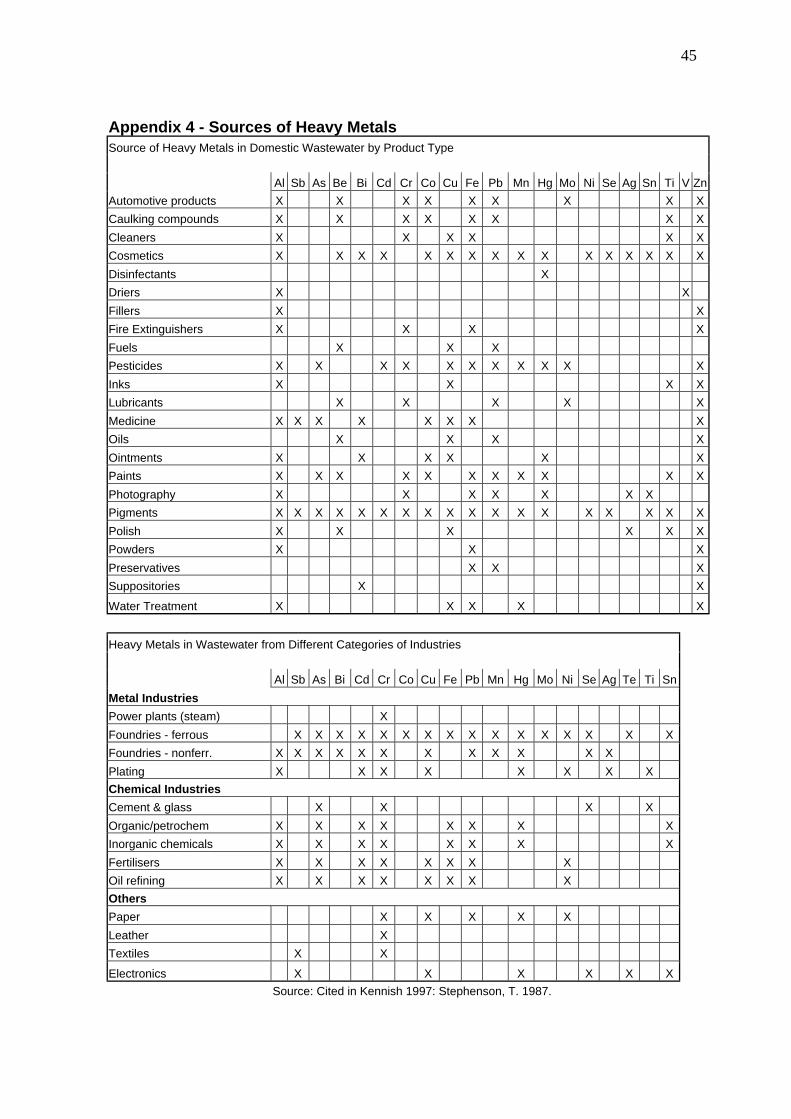
In Appendix 3 the concentrations of the 32 elements considered are given and their use in

domestic or industrial activities is diagrammatically listed in Appendix 4.

The distributions of some of the elements are illustrated in figures 6-17. The ANZECC

guideline values are also present for a visual assessment together with the median value of

each element. Some general comments are also included although these are not exhaustive

and they simply indicate the need for a more detailed analysis of land use and activities in

each sub-catchment where anomalous concentrations are recorded.

In general station CR4A, at the entrance of Cooks River, shows the lowest concentrations.

Major elements

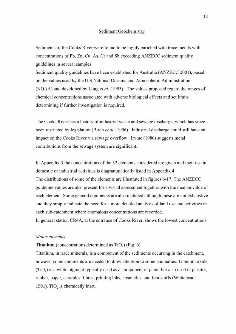
Titanium (concentrations determined as TiO2) (Fig. 6).

Titanium, in trace minerals, is a component of the sediments occurring in the catchment,

however some comments are needed to draw attention to some anomalies. Titanium oxide

(TiO2) is a white pigment typically used as a component of paint, but also used in plastics,

rubber, paper, ceramics, fibres, printing inks, cosmetics, and foodstuffs (Whitehead

1991). TiO2 is chemically inert.

15

Figure 6 – Distribution of titanium concentrations

There are several elevated values of TiO2:

- in the uppermost reaches of the study area, which could be due to the proximity to

local input of industrial runoff contributed by Cup and Saucer Creek;

- at the Tempe boat harbor that may be related to boat cleaning and repair, or waste

from a number of other activities;

- from Alexandra Canal

16

- at station 14 and possibly related to the concentration of vessels at this locality.

Calcium and Magnesium (concentrations determined as MgO and CaO) (Fig. 7)

Whereas magnesium shows comparable concentrations in all stations, calcium shows

three

Figure 7 – Distribution of calcium and magnesiun concentrations

17

main peaks at station CR1, CR7 and CR6A.

Both oxides are connected to the construction industry as CaO, for example, is the main

component of cements and gyprock. Elevated CaO concentrations in Alexandra Canal

could be attributed to cement works near its northern bank.

Phosphate (P2O5) (Fig. 8).

Figure 8 – Distribution of phosphate concentrations

18

Phosphate present in the river sediments is related to excess fertilisers used on parks and

gardens that are washed from soils and into the stormwater system. Values of phosphate

correlate quite well with the land uses surrounding of the river. The relatively high values

correlate well with the surrounding parks and golf course, while lower values are seen

where catchment inputs come from largely developed areas.

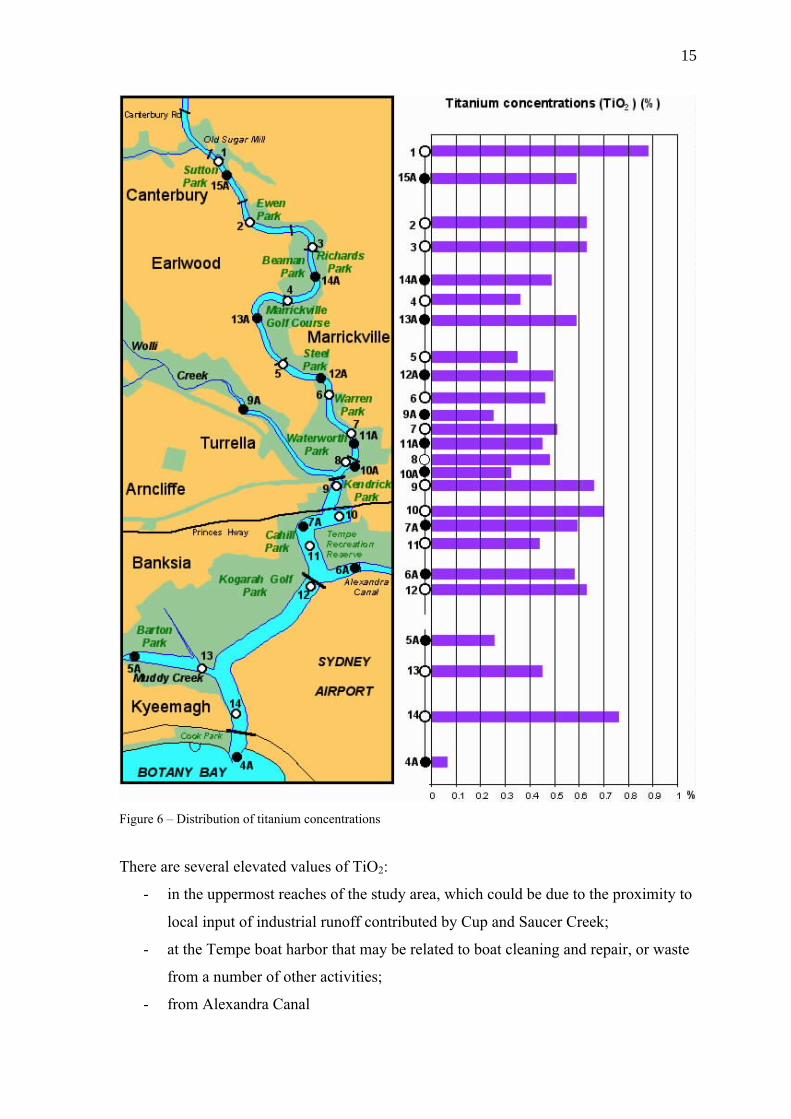
Figure 9 – Distribution of lead concentrations

19

Trace Elements

Lead (Pb) (Fig. 9)

Lead is found in excess of the ANZECC guideline high values in 64% of the samples,

with the highest values at Tempe boat harbour, Alexandra Canal and at station CR14.

This diffuse source of lead is derived from many sources among which Pb-based paints

and vehicular exhaust emissions predominate together with lead-acid batteries and as

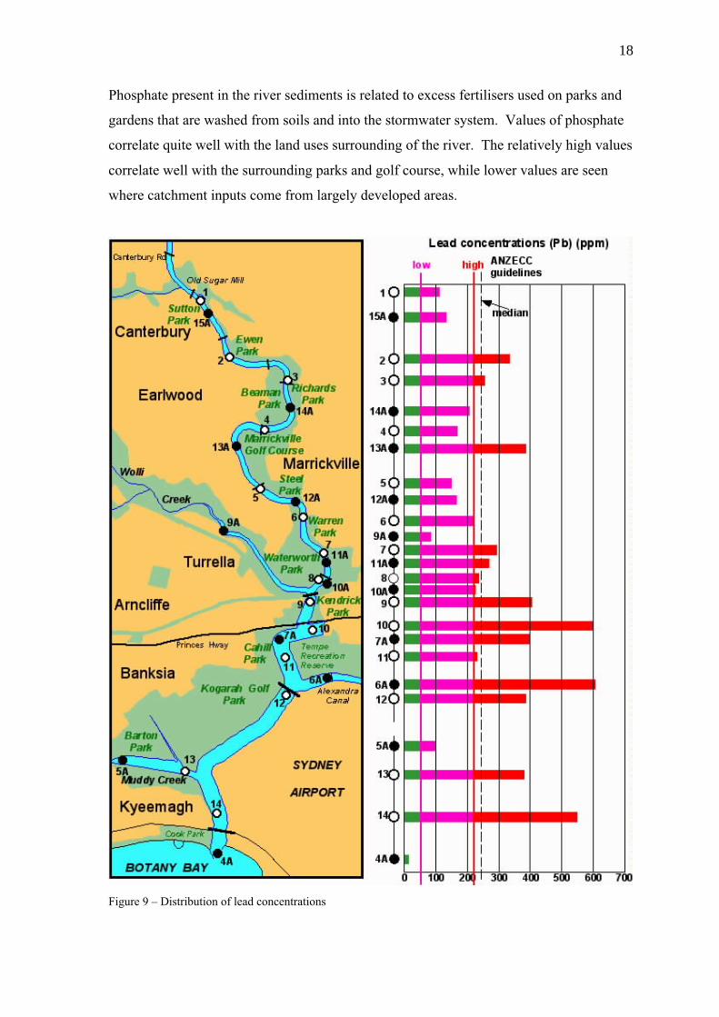
Figure 10 – Distribution of copper concentrations

20

ballast. Additional potential point sources of Pb to Cooks River includes waste dumps,

major sewage overflows and past industrial discharge.

A more detailed analysis of the local activities is required to identify the sources.

Copper (Cu) (Fig. 10)

Both copper and zinc are associated with boating activities, as well as general building

construction and vehicles. Eighteen stations (72%) have a concentration higher than the

“low” ANZECC guideline value. The banning of tributyltin-based antifouling paints may

have lead to increased Cu input into estuarine systems as antifouling paints with higher

Cu content are now used.

While the increased levels of copper in the upper river could be attributed to diffuse

sources, it is likely that the moored boats at Tempe boat harbour, the proximity to some

major road ways including the Princess Highway, and historical discharge of industrial

wastes may be the major impacts elevating copper concentrations

Zinc (Zn) (Fig.11)

Zinc concentrations show a correlation with the inputs suggested for copper but also show

additional input from the river above the study site, and from a number of sub-catchments

within the area. More than half the samples (52%) have a concentration higher that the

“high” value of the ANZECC guidelines. The highest values are at the Tempe boat harbor

and at station CR14; this correlates with the lead distribution. Birch et al. (1996) suggests

that a large group of boats could have a greater input of zinc than stormwater discharge;

high concentrations are associated with slipways, moored boats and sacrificial anodes.

Arsenic (As) (Fig. 12)

Arsenic in its inorganic forms poses a significant toxicity hazard to biota. Assessment of

arsenic in sediments of particular interest as it is believed bottom sediments are the major

source of the metal for benthic communities (Kennish 1997). Arsenic compounds have

been uses in insecticides, herbicides (for railway and power poles), fungicides, algaecides

21

Figure 11 – Distribution of zinc concentrations

and wood preservatives, but such uses are decreasing because of the occupational and

environmental risks (Leonard 1991). Elevated levels of As have been found in some

samples of “green” domestic waste in Australia. Other uses include manufacture of

pigments and antifouling paint, in cosmetics, in the ceramics industry, in fireworks, and in

22

alloys and solders (Leonard 1991). Arsenic impacts can therefore be attributed to

industrial waste discharges.

In Cooks River high values are present at 7 stations (28%) and in particular at the

Alexandra Canal station (stn. CR6A), off the Marrickville Golf Course (stn. CR13A) and

off the drain at Mackey Park (stn. CR11A).

Figure 12 – Distribution of arsenic concentrations

23

Cadmium (Cd) (Fig. 13)

The use of cadmium has greatly increased its input to the environment since the start of

industrialisation, in the form of dust and aerosols into the atmosphere, as effluent into

rivers, and as solids from point sources (wastes, slag, incineration, coal combustion,

phosphate fertilizers, sewage sludge) (Stoeppler 1991). Uses of cadmium include

corrosion protection, Ni-Cd batteries, pigments, soaps, solar cells and various alloys

(Stoeppler 1991).

Figure 13 – Distribution of cadmium concentrations

24

Whereas values observed in the Cooks River are elevated (maximum of approx. 9 ppm at

stn. CR14), its impact of cadmium may not be significant. However 19 stations (76%) are

above the “low” ANZECC value. Note of consideration is the presence of the highest

values (8-9 ppm) at stations CR6 (Alexandra Canal) and CR3; additional locations (CR10

and CR14) appears to be related to the presence of boating activity.

Figure 14 – Distribution of chromium concentrations

25

Chromium (Cr) (Fig. 14)

Most of the chromium produced is used in the metal industry, in alloys and steels

(stainless steel), and in the galvanizing industry for chrome plating (Gauglhofer and

Bianchi 1991). Loss to the environment during production is possible as dust, liquid or

aerosol. Other uses include as pigments, as a catalyst and in the tanning industry

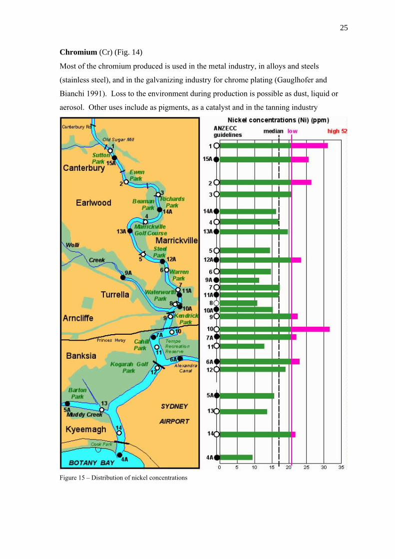
Figure 15 – Distribution of nickel concentrations

26

(Gauglhofer and Bianchi 1991), from which chromium can escape into the environment

via effluent. The values seen in the river are significant due to their order of magnitude; 9

samples (36%) have a value higher that the “low” ANZECC value but only one (CR5A)

exceeds the “high” value.

Nickel (Ni) (Fig. 15)

Nickel enters the estuarine environment from a variety of natural and industrial sources

including waste disposal (Sunderman and Oskaarsson 1991). In Cooks River 9 stations

(36%) show a concentration higher than the “low” ANZECC value; stations CR10

(Tempe boat harbour) and CR1 have the highest values, but still well below the “high”

ANZECC value.

Tin (Sn) (Fig. 16)

Tin is used to coat other metals to prevent corrosion and some components are biocides.

The concentrations of tin in Cooks River show 3 main peaks (CR15A, CR4 and CR9) that

appear to be related to some anthropogenic activity not clearly identified.

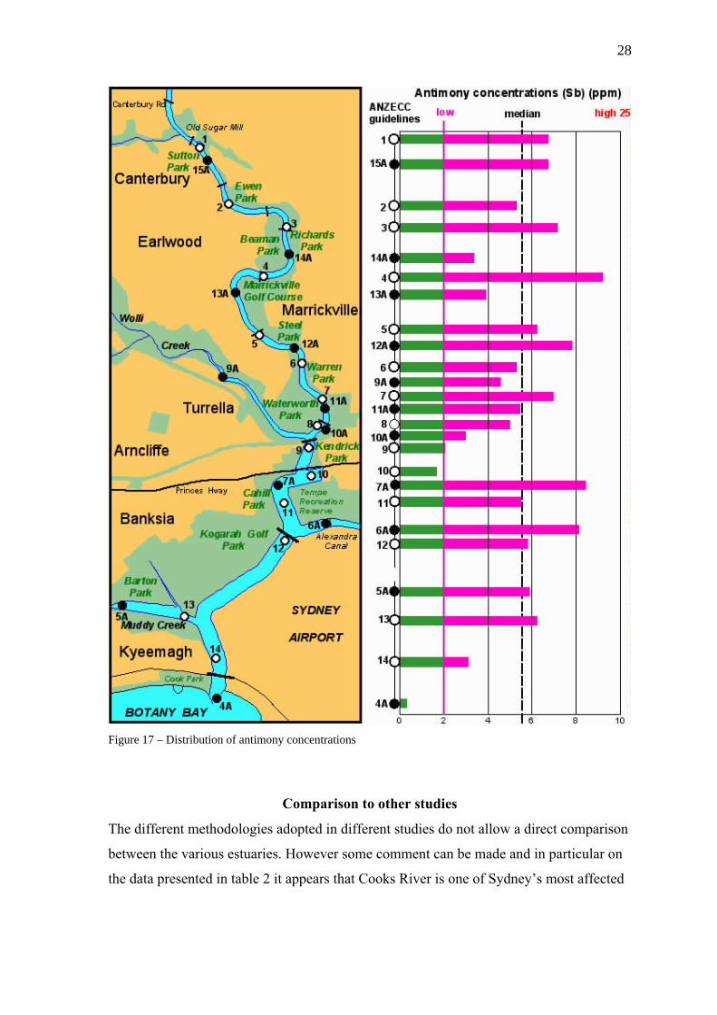
Antimony (Sb) (Fig. 17)

Antimony and many of its components are toxic. It is used in a great variety of industries

from semiconductors to flame-retardant formulations. As an alloy it increases the

hardness of lead and, as such, is used for storage batteries. Other uses include ceramic

enamels, paints and pottery.

Many of the trace elements display strong correlations in their concentrations. This may

be related to either common pollution source or variations in the distribution of minerals

capable of trapping these trace metals in sediment along the river.

The specific uses of the trace metals not described above can be found in Appendix 4.

Industrial uses such as in alloy/steel manufacture, in plating industries, in fertilisers, as

pigments and colourings, as wood preservatives, as catalysts, in production of ceramics

and glass, for electronics and in medical applications. A detailed analysis of current and

past industrial activities in the catchment would allow a better determination of the source

of these trace metals.

27

The data here presented form a base-line reference for more detailed analysis of the land

use, past and present, in order to assess the level of anthropogenic impact on Cooks River.

Figure 16 – Distribution of tin concentrations

28

Figure 17 – Distribution of antimony concentrations

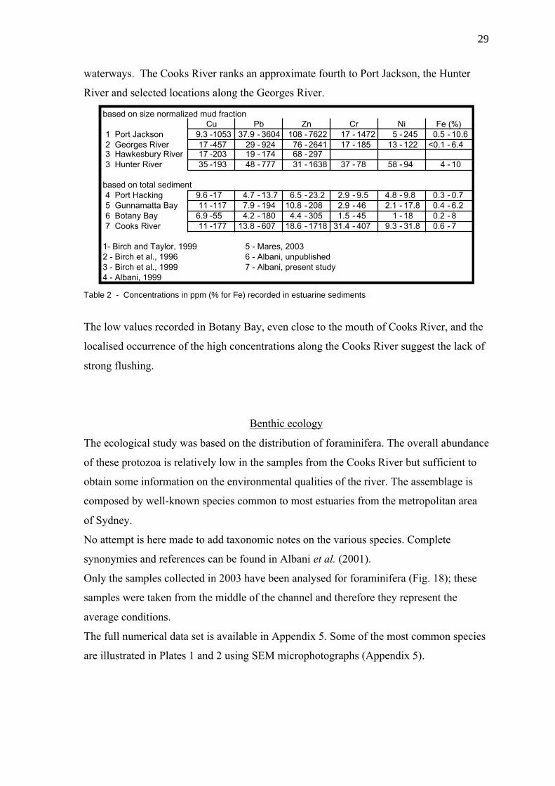
Comparison to other studies

The different methodologies adopted in different studies do not allow a direct comparison

between the various estuaries. However some comment can be made and in particular on

the data presented in table 2 it appears that Cooks River is one of Sydney’s most affected

29

waterways. The Cooks River ranks an approximate fourth to Port Jackson, the Hunter

River and selected locations along the Georges River.

based on size normalized mud fractionCu Pb

----

----

Zn----

----

Cr--

-

----

Ni--

-

----

Fe (%)--

-

----

1 Port Jackson 9.3171735

9.611

6.911

----

----

1053457203193

1711755177

37.9291948

4.77.94.2

13.8

3604924174777

13.7194180607

108766831

6.510.8

4.418.6

762226412971638

23.22083051718

1717

37

2.92.91.5

31.4

1472185

78

9.54645407

513

58

4.82.1

19.3

245122

94

9.817.81831.8

0.5<0.1

4

0.30.40.20.6

10.66.4

10

0.76.287

2 Georges River3 Hawkesbury River3 Hunter River

based on total sediment4 Port Hacking5 Gunnamatta Bay6 Botany Bay7 Cooks River

1- Birch and Taylor, 1999 5 - Mares, 20032 - Birch et al., 1996 6 - Albani, unpublished3 - Birch et al., 1999 7 - Albani, present study4 - Albani, 1999

Table 2 - Concentrations in ppm (% for Fe) recorded in estuarine sediments

The low values recorded in Botany Bay, even close to the mouth of Cooks River, and the

localised occurrence of the high concentrations along the Cooks River suggest the lack of

strong flushing.

Benthic ecology

The ecological study was based on the distribution of foraminifera. The overall abundance

of these protozoa is relatively low in the samples from the Cooks River but sufficient to

obtain some information on the environmental qualities of the river. The assemblage is

composed by well-known species common to most estuaries from the metropolitan area

of Sydney.

No attempt is here made to add taxonomic notes on the various species. Complete

synonymies and references can be found in Albani et al. (2001).

Only the samples collected in 2003 have been analysed for foraminifera (Fig. 18); these

samples were taken from the middle of the channel and therefore they represent the

average conditions.

The full numerical data set is available in Appendix 5. Some of the most common species

are illustrated in Plates 1 and 2 using SEM microphotographs (Appendix 5).

30

Figure 18 – Sample location for foraminiferal study

While the sediment study offers an understanding of the clastic inputs of the various sub

catchments, there is no indication of the age of such occurrences. The foraminiferal study,

however, has the capacity to add a partial time factor as the technique adopted limits the

age of the samples to the last 3-5 years. The correlation between sediment and

foraminiferal abundance allows, therefore, distinguishing the events of the last 3-5 years

from previous events.

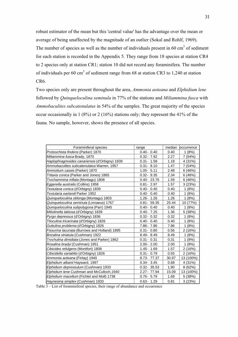
All foraminifera present in the samples were identified and counted; the total assemblage,

composed by 29 benthic foraminiferal species, is listed in table 3. Each species is

recorded with their range of abundance, the median value and occurrence, expressed as

the number of stations where they occur as well as percentage area. The median is a

31

robust estimator of the mean but this 'central value' has the advantage over the mean or

average of being unaffected by the magnitude of an outlier (Sokal and Rohlf, 1969).

The number of species as well as the number of individuals present in 60 cm3 of sediment

for each station is recorded in the Appendix 5. They range from 18 species at station CR4

to 2 species only at station CR1; station 10 did not record any foraminifera. The number

of individuals per 60 cm3 of sediment range from 68 at station CR3 to 1,240 at station

CR6.

Two species only are present throughout the area, Ammonia aoteana and Elphidium lene

followed by Quinqueloculina seminula in 77% of the stations and Miliammina fusca with

Ammobaculites subcatenulatus in 54% of the samples. The great majority of the species

occur occasionally in 1 (8%) or 2 (16%) stations only; they represent the 41% of the

fauna. No sample, however, shows the presence of all species.

Foraminiferal species range median occurrenceProtoschista findens (Parker) 1870 0.40- 0.40 0.40 1 (8%)Miliammina fusca Brady, 1870 0.32- 7.92 2.27 7 (54%)Haplophragmoides canariensis (d'Orbigny) 1839 0.31- 1.58 1.18 4 (31%)Ammobaculites subcatenulatus Warren, 1957 0.31- 8.10 1.47 7 (54%)Ammotium cassis (Parker) 1870 1.05- 5.11 2.48 6 (46%)Tritaxis conica (Parker and Jones) 1865 0.32- 9.35 2.34 6 (46%)Trochammina inflata (Montagu) 1808 0.40- 23.76 1.59 6 (46%)Eggerella australis (Collins) 1958 0.81- 2.97 1.57 3 (23%)Textularia conica (d'Orbigny) 1839 0.40- 0.40 0.40 1 (8%)Textularia earlandi Parker 1952 0.40- 0.40 0.40 1 (8%)Quinqueloculina oblonga (Montagu) 1803 1.26- 1.26 1.26 1 (8%)Quinqueloculina seminula (Linnaeus) 1767 0.81- 59.35 25.44 10 (77%)Quinqueloculina subpolygona (Parr) 1945 0.40- 0.40 0.40 1 (8%)Miliolinella labiosa (d'Orbigny) 1839 0.40- 7.25 1.36 5 (38%)Pyrgo depressus (d'Orbigny) 1836 0.32- 0.32 0.32 1 (8%)Tiloculina tricarinata (d'Orbigny) 1826 0.40- 0.40 0.40 1 (8%)Guttulina problema (d'Orbigny) 1826 7.86- 7.86 7.86 1 (8%)Fissurina lacunata (Burrows and Holland) 1895 0.31- 0.80 0.56 2 (16%)Brizalina striatula (Cushman) 1922 8.49- 8.49 8.49 1 (8%)Trochulina dimidiata (Jones and Parker) 1862 0.31- 0.31 0.31 1 (8%)Rosalina bradyi (Cushman) 1951 2.00- 2.00 2.00 1 (8%)Cibicides refulgens (Montfort) 1808 1.45- 1.69 1.57 2 (16%)Cibicidella variabilis (d'Orbigny) 1826 0.31- 0.79 0.55 2 (16%)Ammonia aoteana (Finlay) 1940 8.73- 77.37 30.97 13 (100%)Elphidium albanii Hayward, 1997 0.34- 3.45 0.68 4 (31%)Elphidium depressulum (Cushman) 1933 0.32- 35.53 1.90 8 (62%)Elphidium lene Cushman and McCulloch,1940 2.27- 77.94 15.09 13 (100%)Elphidium macellum (Fichtel and Moll) 1738 0.76- 5.79 1.69 5 (38%)Haynesina simplex (Cushman) 1933 0.63- 1.29 0.81 3 (23%)

Table 3 – List of foraminiferal species, their range of abundance and occurrence

32

Species diversity increases downstream from station 1 to station 4A suggesting an

improvement of nutrients availability. The high diversity value of 16 species was

recorded at station 4 indicating the presence of the highest nutrients load. The density of

population, however, correlates well with recent sediment inputs; for example, stations 2

and 3 appear to show similar water qualities but the low abundance of individuals at

station 3 strongly indicates the presence of sediment input higher that that at station 2.

In figure 19 the number of species and the numbers of individuals are plotted against the

station locations

Figure 19 – Distribution of number of species and number of individuals

Note that the density of population at station 4 is relatively low suggesting some sediment

input, comparable with that of stations 8, 12 and 4A. Stations 5, 6 and 11, on the contrary,

indicate the presence of limited sediment input.

33

The species abundance expressed as percentage of the assemblage of each station

(Appendix 5) form the numeric data set has been used to determine the level of similarity

between samples. Cluster analysis has been applied to the total data set using the Pearson

correlation coefficient to generate the similarity matrix, graphically shown as a

dendrogram (fig. 20).

The geographic distribution of the various clusters (Fig. 21), defined as biotopes, can be

identified in terms of their faunal composition and they tend to describe the predominant

water qualities and characteristics; the main processes are the tidal flows and the extent of

inputs from the various sub catchments.

Figure 20 – Dendrogram of the cluster analysis (Pearson coefficient)

Inner Estuarine Biotope – This Biotope occupies the most inner portion of the River. It is

primarily affected by the surface runoff of the main catchment. Note the presence of this

biotope at station 13 suggesting a similar input from Muddy Creek and its catchment.

It is composed predominantly by Ammonia aoteana and Elphidium lene with occasional

presence of Trochammina inflata, which is a typical species found mainly in brackish

environments.

Outer Estuarine Biotope – Quinqueloculina seminula and Ammonia aoteana with minor

presence of Elphidium lene form the main assemblage of this Biotope that reflects the

marginal influence of the tidal flow. It shows a greater species diversity as well as a

greater number of individuals that the previous biotope. Station 4, with its maximum

number of species, belongs to this biotope.

34

Figure 21 – Geographic distribution of the foraminiferal Biotopes

Inner Tidal Biotope – This Biotope may reflect the most upstream reach of the tidal

influence from Botany Bay. Ammonia aoteana is the most abundant followed by

Elphidium lene and a number of species generally found in estuarine-marine conditions

such as Elphidium depressulum, Elphidium macellum and Quinqueloculina seminula.

Station 12 shows the presence of Tritaxis conica and Trochammina inflata, these two

species are generally typical of brackish environment suggesting perhaps some input from

the Alexandra Canal.

Outer Tidal Biotope – It is composed by only one station with a distinct assemblage.

Elphidium depressulum, Ammonia aoteana and Elphidium lene together with a number of

species typical of the marine conditions such as Guttulina problema, Quinqueloculina

seminula, Quinqueloculina oblonga, Brizalina striatula and others.

Its location at the mouth of the River justifies the more marine nature of the assemblage.

35

Conclusions

The present study offers an overall assessment of the present status of Cooks River, thus

the data here presented can be used as base line for further monitoring.

Several of the anomalous occurrences of sediment types and heavy metals require further

investigation to establish their source, to eliminate or minimise any further inputs and to

establish the remedial work necessary to restore the optimal natural conditions.

In addition, understandings of the changes that have occurred since the urbanisation of the

area would be elucidate some of the anomalies. Such chronologically oriented study can

be conducted by using a number of cores, instead of surface samples. The presence of

benthic foraminifera would allow some absolute age determinations and therefore it

would reconstruct the history of Cooks River.

36

References

Albani, A.D., 1968. Recent Foraminiferida from Port Hacking, New South Wales.Contribution of the Cushman Foundation for Foraminiferal Research, 19: 85-119.

Albani, A.D., 1974. Sedimentary environments in Broken Bay, N.S.W., Australia.Journal of the Geological Society of Australia, 21: 277-288

Albani, A.D., 1978. Recent foraminifera of an estuarine environment in Broken Bay, NewSouth Wales. Australian Journal of Marine and Freshwater Research, 29: 355-398.

Albani, A.D., 1979. Recent Shallow Water Foraminiferida from New South Wales.AMSA Handbook no.3, Australian Marine Sciences Association., Sydney, 57 pp.

Albani, A.D. 1993. Use of benthonic foraminifera to evaluate the environmentalcharacteristics of Port Hacking; significance for coastal engineering works andpollution. In G. McNally, M. Knight, & R. Smith (Eds.), Collected Case Studies inEngineering Geology, Hydrogeology and Environmental Geology (pp. 134).Geological Society of Australia: Sydney.

Albani, A.D. 1999. Port Hacking: tidal delta sediment study. The Hacking RiverCatchment Committee.

Albani, A.D., and Brown, G.A., 1976. Geological Contribution to EnvironmentalManagement of Coastal Lagoons at Gosford, N.S.W. (Australia). Bulletin of theInternational Association of Engineering Geology, 14: 84-104.

Albani, A.D., Favero, V. and Serandrei Barbero, R. 1984. Benthonic foraminifera asindicators of intertidal environments. Geo-marine Letters, 4 : 43-47.

Albani, A.D., Favero, V. and Serandrei Barbero, R. 1991b. The distribution andecological significance of Recent Foraminifera in the Lagoon south of Venice.Revista Espanola de Micropaleontologia, 23 (2): 129-143.

Albani, A.D., Favero, V. and Serandrei Barbero, R., 1998 - Distribution of Sediment andBenthic Foraminifera in the Gulf of Venice, Italy. Estuarine, Coastal and ShelfScience, 46 (2): 252-265

Albani, A.D., Rickwood, P.C., Favero, V. and Serandrei Barbero, R., 1989 - Thegeochemistry of marine sediments off the Lagoon of Venice. Bulletin of MarinePollution, 20 (9): 438-442

Albani, A.D., Rickwood, P.C., Favero, V.M. and Serandrei Barbero, R. 1989b. Thegeochemical anomalies in sediments on the shelf near the Lagoon of Venice, Italy.Marine Pollution Bulletin, 20 (9): 438-442.

Albani, A.D., Rickwood, P.C., Favero, V.M. and Serandrei Barbero, R. 1995. Thegeochemistry of recent sediments in the Lagoon of Venice: environmentalimplications. Istituto Veneto di Scienze, Lettere ed Arti, Atti, 153 pp.

Albani, A. D., Rickwood, P.C., Nielsen, L. and Lord, D. 1991a. Geological andHydrodynamic Conditions in Broken Bay, New South Wales. TechnicalContribution Series. 1. Centre for Marine Science, University N.S.W.: Sydney.

Albani, A.D., Hayward, B.W., Grenfell, H.R. and Lombardo, R. 2001. Foraminifera fromthe South West Pacific. Australian Biological Resources Study.Interactive CD-ROM.

Alve, E. 1995. Benthic foraminiferal responses to estuarine pollution: a review. Journalof Foraminiferal Research 25:190-203.

ANZECC. Australian & New Zealand Environment and Conservation Council andAgricultural & Resource Council of Australia New Zealand. 2001. National Water

37

Quality Management Strategy – Draft Guidelines for Urban StormwaterManagement, Paper 4, Volume 1.

Armynot du Chatelet, E., Debenay, J.P. and Soulard, R., 2004. Foraminiferal proxies forpollution monitoring in moderately polluted harbors. Environmental Pollution 127:27-40.

Birch, G.F., Evenden, D., and Teutsch, M.E., 1996. Dominance of point source in heavymetal distributions in sediments of a major Sydney Estuary (Australia).Environmental Geology 28: 69-174.

Birch, G.F., Eyre, B.D. and Taylor, S.E., 1999. The use of sediments to assessenvironmental impact on large coastal catchment – the Hawkesbury River system.AGSO Journal of Australian Geology & Geophysics 17 (5/6):175-191.

Birch, G.F. and Taylor, S.E., 1999. Source of heavy metals in sediments of the PortJackson estuary, Australia. Science of the Total Environment 277 pp123-138.

Irvine, I. 1980. Sydney Harbour: sediments and heavy metal pollution. PhD thesis,University of Sydney. Unpublished

Johnson, K.R. and Albani, A.D. 1973. Biotopes of Recent benthonic foraminifera in PittWater, Broken Bay, N.S.W. Palaeogeography, Palaeoclimatology, Palaeoecology,14 : 265-276.

Keenish, M. J., 1997. Heavy metals. In: Practical Handbook of Estuarine and MarinePollution. CRC Press, Boca Raton.

Kollias, G., 2004. A catchment-based environmental impact assessment of the CooksRiver, Sydney: sediment and trace metal impacts. Honours Thesis, University ofNew South Wales. Unpublished.

Leonard, A. 1991. Arsenic. In: Metals and Their Compounds in the Environment.Merian, E., Ed. VCH Publishers, New York. pp751-774.

Long E.R., MacDonald D.D., Smith S.L. and Calder E.D. 1995. Incidence of adversebiological effects within ranges of chemical concentrations in marine and estuarinesediments. Environment Management 19: 81–97.

Mares, T. 2003. Gunnamatta Bay. Honours Thesis, University of New South Wales.Unpublished.

Rickwood, P.C. 1983. Cluster analysis of geochemical data. In S.S. Augustithis (Eds.),The Significance of Trace Elements in Solving Petrogenetic Problems andControversies (pp. 116-124). Theophrastus Publications S.A.: Athens.

Rickwood, P.C., Albani, A.D. and Chorley, G.I. 1983. The relationship between sedimentcomposition and the distribution of benthic foraminifera in Broken Bay, New SouthWales, Australia. In S.S. Augustithis (Eds.), The Significance of Trace Elements inSolving Petrogenetic Problems and Controversies (pp. 135-147). TheophrastusPublications S.A.: Athens.

Rickwood, P.C., Albani, A.D., Favero, V.M. and Serandrei Barbero, R. 1992. Thegeochemistry of unconsolidated sediments from the Gulf of Venice, Italy. TechnicalContribution Series. 3. Centre for Marine Science, University N.S.W.: Sydney.

Serandrei Barbero, R., Albani, A.D. and Favero, V.M. 1989. Distribuzione deiforaminiferi recenti nella Laguna di Venezia. Bollettino della Società GeologicaItaliana, 108 : 279-288.

Sokal, R.R., Rohlf, F.J., 1969. Biometry. W.H. Freeman and Company, San Francisco,776 pp.

Stephenson, T. 1987. Sources, analysis, and legislation. In: Heavy Metals in Wastewaterand Sludge Treatment Processes, Vol. 1. Lester, J.N (Ed.), CRC Press, Boca Raton.pp46.

Stoeppler, M. 1991. Cadmium. In: Metals and Their Compounds in the Environment.Merian, E., Ed. VCH Publishers, New York. pp 803-851. Gauglhofer, J. and

38

Bianchi, V. Chromium. In: Metals and Their Compounds in the Environment.Merian, E., Ed. VCH Publishers, New York. pp853-878.

Sunderman, F.W. and Oskaarsson, A. 1991. In: Metals and Their Compounds in theEnvironment. Merian, E., Ed. VCH Publishers, New York. pp 1101-1126.

39

Appendix 1 – Sediments grain size data

Appendix 2 – Sediments grain size graphic parameters

Appendix 3 – Geochemical data

Appendix 4 – Most common sources of heavy metals

Appendix 5 – Benthic foraminifera

40

Appendix 1 - Sediment grain size (in phi and mm values)phi mm CR01 CR02 CR03 CR04 CR04A CR05 CR05A CR06 CR06A CR07 CR07A-2.00 4.00 0.00 0.00 0.00 1.03 0.00 2.94 0.00 4.26 0.00 2.71 0.00-1.75 3.36 2.67 0.00 0.00 0.23 0.00 0.53 0.00 1.40 0.00 0.75 0.00-1.50 2.83 2.79 0.04 0.34 0.83 0.00 0.21 0.16 2.64 1.17 1.31 0.69-1.25 2.38 3.15 0.22 0.51 0.33 0.00 0.51 0.16 2.19 3.27 0.45 1.61-1.00 2.00 5.16 0.04 0.34 0.01 0.00 0.71 0.15 1.37 1.65 0.69 1.00-0.75 1.68 3.70 0.09 0.83 0.14 0.06 0.45 0.35 3.36 2.12 0.76 1.76-0.50 1.41 3.05 0.29 1.29 0.15 0.03 0.88 0.19 3.29 1.72 1.18 1.78-0.25 1.19 3.18 0.21 1.26 1.25 0.02 0.99 0.18 2.82 1.40 1.06 1.230.00 1.00 3.75 0.27 1.39 1.05 0.07 1.70 0.18 3.33 1.21 1.04 1.070.25 0.84 4.89 0.41 1.41 2.20 0.13 2.63 0.28 4.18 1.70 1.33 1.490.50 0.71 5.43 0.53 1.84 4.55 0.16 6.29 0.49 5.81 1.02 2.27 0.750.75 0.59 9.92 1.04 2.45 10.09 0.32 12.04 0.58 7.65 1.27 3.37 0.791.00 0.50 7.96 2.52 3.99 16.56 2.57 17.23 3.02 11.05 2.31 6.97 1.971.25 0.42 11.02 3.11 10.11 11.09 6.24 9.20 6.06 7.62 1.56 6.95 1.791.50 0.35 3.42 5.61 12.87 10.74 17.74 8.70 21.57 10.57 2.19 11.69 3.331.75 0.30 11.64 2.75 9.18 3.13 21.68 2.69 18.22 3.57 2.38 5.69 3.902.00 0.25 2.59 16.51 9.73 6.34 19.96 4.57 12.63 7.52 1.50 17.09 3.132.25 0.21 1.24 9.13 3.21 1.68 21.89 1.16 22.15 1.48 2.53 5.89 8.252.50 0.18 0.35 5.27 2.57 1.19 5.66 0.86 6.59 1.04 1.28 4.66 5.322.75 0.15 0.34 0.96 1.42 0.64 0.01 0.56 0.05 0.85 0.38 2.25 0.633.00 0.12 0.38 0.71 0.74 0.44 0.03 0.30 0.13 0.46 1.15 0.55 1.233.25 0.11 0.47 0.91 0.79 0.35 0.04 0.28 0.20 0.54 1.87 0.38 1.843.58 0.08 0.56 1.19 1.09 0.52 0.06 0.38 0.26 0.67 2.49 0.52 2.193.85 0.07 0.61 1.50 1.37 0.70 0.07 0.48 0.30 0.78 2.93 0.68 2.644.13 0.06 0.68 1.80 1.75 0.94 0.09 0.63 0.33 0.88 3.23 0.83 2.744.40 0.05 0.74 2.12 1.90 1.11 0.10 0.72 0.35 0.85 3.37 1.04 2.724.68 0.04 0.80 2.41 2.09 1.28 0.10 0.85 0.36 0.85 3.48 1.10 2.774.95 0.03 0.86 2.66 2.17 1.42 0.11 0.98 0.37 0.82 3.56 1.20 2.815.50 0.02 1.88 5.63 4.38 3.19 0.25 2.36 0.74 1.55 7.52 2.65 5.866.05 0.02 1.97 5.82 4.20 3.40 0.29 2.80 0.76 1.44 8.17 2.61 6.436.61 0.01 1.69 5.36 3.64 3.23 0.34 2.93 0.74 1.24 8.08 2.34 6.557.16 0.01 1.19 4.85 2.91 2.78 0.37 2.80 0.67 1.00 6.93 1.98 5.817.98 0.004 1.00 5.95 3.16 3.09 0.54 3.73 0.76 1.12 7.18 2.41 6.439.09 0.002 0.57 5.56 2.70 2.47 0.56 3.51 0.59 0.96 5.24 2.04 5.22

10.18 0.001 0.27 3.49 1.72 1.35 0.37 1.82 0.33 0.59 3.13 1.14 3.3111.02 0.0005 0.10 1.03 0.65 0.47 0.13 0.59 0.09 0.23 1.00 0.41 0.95

12.29 0.0002 0.00 0.00 0.01 0.01 0.00 0.01 0.00 0.01 0.00 0.01 0.00

41

Appendix 1 (cont.) - Sediment grain size (in phi and mm values)phi mm CR09 CR10 CR10A CR11 CR11A CR12 CR13 CR13A CR14 CR14A CR15A-2.00 4.00 3.23 0.00 0.00 0.09 0.00 0.46 0.86 0.00 0.07 0.00 0.00-1.75 3.36 1.90 0.00 0.00 0.00 0.00 0.00 0.00 0.00 0.00 0.00 0.00-1.50 2.83 1.07 0.46 2.88 0.00 0.78 0.16 0.00 3.38 0.00 0.24 2.41-1.25 2.38 0.96 0.20 7.41 0.00 0.68 0.27 0.24 5.80 0.00 0.61 5.41-1.00 2.00 0.54 0.00 5.29 0.02 1.36 0.10 0.04 4.39 0.00 1.41 3.90-0.75 1.68 1.21 0.03 8.12 0.00 1.29 0.09 0.06 4.29 0.03 1.47 6.54-0.50 1.41 1.84 0.00 5.30 0.03 1.19 0.12 0.09 3.86 0.07 0.99 4.33-0.25 1.19 2.08 0.00 4.16 0.03 1.48 0.10 0.05 2.40 0.04 1.18 3.220.00 1.00 1.37 0.00 4.27 0.02 1.00 0.12 0.09 3.07 0.02 1.22 3.840.25 0.84 1.44 0.03 4.63 0.06 1.67 0.11 0.07 3.87 0.03 2.51 4.610.50 0.71 1.81 0.00 3.39 0.10 2.55 0.13 0.14 2.19 0.03 1.72 3.850.75 0.59 2.63 0.04 3.44 0.11 1.77 0.25 0.24 2.69 0.06 1.85 3.431.00 0.50 3.70 0.06 9.23 0.67 5.16 0.47 0.49 6.50 0.16 6.80 9.351.25 0.42 2.59 0.09 8.55 0.79 5.38 1.21 0.89 5.55 0.08 6.24 8.621.50 0.35 3.30 0.19 11.82 2.70 9.14 0.60 2.41 7.17 0.22 8.51 11.051.75 0.30 1.05 0.09 7.57 2.76 6.81 8.25 1.47 3.82 0.10 4.86 7.482.00 0.25 3.66 0.37 3.41 15.29 4.67 4.77 16.21 2.95 0.68 4.28 7.052.25 0.21 1.31 0.30 3.23 13.23 11.02 6.60 18.24 4.06 1.42 5.62 6.762.50 0.18 1.17 0.29 0.87 18.21 7.37 3.91 11.19 2.30 0.62 2.71 2.862.75 0.15 1.14 1.87 0.01 12.50 0.02 3.20 6.08 0.00 1.86 0.00 0.023.00 0.12 0.74 2.50 0.07 3.76 0.45 1.78 2.13 0.18 2.14 0.22 0.073.25 0.11 1.05 3.01 0.11 1.08 0.87 2.32 1.07 0.41 2.49 0.58 0.123.58 0.08 1.37 3.66 0.16 1.27 1.13 2.87 1.23 0.61 2.99 0.90 0.153.85 0.07 1.68 4.14 0.18 1.41 1.33 3.18 1.39 0.78 3.48 1.16 0.184.13 0.06 2.06 4.46 0.21 1.73 1.45 3.48 1.51 1.01 4.06 1.40 0.194.40 0.05 2.29 4.49 0.24 1.60 1.47 3.49 1.48 1.09 4.17 1.59 0.204.68 0.04 2.56 4.60 0.27 1.65 1.47 3.50 1.56 1.24 4.44 1.77 0.214.95 0.03 2.81 4.47 0.29 1.67 1.45 3.43 1.61 1.36 4.69 2.04 0.215.50 0.02 6.27 8.37 0.67 3.36 2.93 6.80 3.48 3.09 10.03 4.20 0.466.05 0.02 7.05 8.32 0.73 3.32 3.34 7.02 3.99 3.65 11.04 4.82 0.516.61 0.01 7.09 8.29 0.70 2.94 3.74 6.74 4.22 3.85 10.23 5.25 0.557.16 0.01 6.70 8.31 0.62 2.43 3.62 6.08 4.05 3.57 8.60 5.29 0.537.98 0.004 7.89 10.90 0.75 2.76 4.76 7.25 5.14 4.15 9.84 6.92 0.679.09 0.002 6.94 11.07 0.74 2.40 4.58 6.17 4.65 3.59 8.97 6.37 0.65

10.18 0.001 4.06 6.90 0.50 1.47 3.06 3.61 2.70 2.35 5.45 3.94 0.4411.02 0.0005 1.42 2.42 0.17 0.55 1.00 1.31 0.92 0.79 1.89 1.34 0.14

12.29 0.0002 0.03 0.04 0.00 0.01 0.00 0.03 0.02 0.00 0.03 0.01 0.00

42

Appendix 2 - Sediments graphic parameters

Station CR01 CR02 CR03 CR04 CR04A CR05 CR05A CR06 CR06AMean Mz 0.63 4.02 2.93 2.5 1.78 2.48 1.75 0.83 4.22Standard deviation SD 1.85 2.59 2.45 2.4 0.34 2.77 0.79 1.95 3.18Skewness Sk 0.09 0.46 0.59 0.72 0.06 0.68 0.39 0.1 -0.22Kurtosis K 1.78 0.79 0.95 1.07 1.14 1.75 2.4 1.93 0.87

Station CR07 CR07A CR08 CR09A CR10 CR10A CR11 CR11A CR12Mean Mz 2.52 4.13 3.1 1.07 6.02 0.48 3.3 3.23 4.67Standard deviation SD 2.41 2.9 2.13 1.46 2.21 1.62 1.84 2.75 2.66Skewness Sk 0.37 0.04 0.7 0.42 0.1 -0.03 0.7 0.63 0.04Kurtosis K 2.58 0.89 2.55 3.33 0.86 1.24 1.29 0.85 0.82

Station CR12A CR13 CR13A CR14 CR14A CR15A CRO9 Mean Mz 1.05 3.73 2.22 5.85 3.2 0.72 4.25 Standard deviation SD 2.08 2.32 3.26 2.11 3.32 1.42 3.49 Skewness Sk 0.19 0.78 0.42 0.09 0.4 -0.14 -0.2

Kurtosis K 1.88 0.83 0.78 1 0.74 1.02 0.81

43

Appendix 3 - Geochemical data, major elements (%)station SiO2 TiO2 Al2O3 Fe2O3 MnO MgO CaO Na2O K2O P2O5 SO3

CR01 69.74 0.94 10.57 6.73 0.06 2.75 4.09 2.54 1.42 0.31 0.85CR02 75.95 0.70 9.91 4.36 0.26 1.59 1.45 2.08 1.07 0.19 2.45CR03 77.57 0.68 9.74 4.03 0.03 1.44 1.67 2.10 1.09 0.23 1.42CR04 85.11 0.39 5.91 2.57 0.01 0.86 1.22 1.50 0.61 0.12 1.70CR04A 96.61 0.06 0.73 0.99 0.01 0.15 0.36 0.69 0.25 0.03 0.11CR05 85.43 0.37 5.17 2.47 0.01 0.70 2.46 1.32 0.49 0.13 1.44CR05A 90.66 0.28 2.93 2.01 0.03 0.62 0.88 1.22 0.51 0.12 0.75CR06 77.56 0.50 8.51 4.43 0.03 1.28 2.44 2.30 1.12 0.23 1.59CR06A 59.34 0.76 12.99 6.00 0.04 2.03 10.03 3.40 1.25 0.28 3.89CR07 76.69 0.57 7.30 3.68 0.03 1.42 5.70 2.09 0.88 0.22 1.42CR07A 70.58 0.76 11.27 4.77 0.04 1.65 3.17 3.64 1.04 0.31 2.78CR08 86.17 0.51 5.14 2.55 0.02 0.89 1.34 1.57 0.63 0.14 1.03CR09 64.44 0.81 14.17 6.41 0.04 2.01 3.34 3.41 1.47 0.27 3.61CR09A 88.60 0.27 3.00 2.01 0.02 0.48 2.22 1.41 0.30 0.15 1.54CR10 63.66 0.85 15.53 6.88 0.04 2.02 1.91 3.28 1.52 0.30 4.01CR10A 88.79 0.33 3.95 2.35 0.02 0.70 1.18 1.20 0.64 0.11 0.72CR11 84.76 0.47 5.82 2.89 0.02 1.06 1.21 1.82 0.76 0.18 1.00CR11A 82.70 0.49 6.23 3.47 0.04 1.05 2.19 1.73 0.92 0.17 1.02CR12 72.05 0.76 10.81 5.21 0.04 1.81 2.18 3.24 1.17 0.28 2.44CR12A 81.99 0.53 6.26 3.86 0.04 1.31 2.64 1.68 0.99 0.23 0.48CR13 81.65 0.51 7.06 3.02 0.02 1.29 1.34 2.34 0.92 0.18 1.66CR13A 73.43 0.68 11.26 4.89 0.04 1.51 1.57 2.68 1.27 0.23 2.45CR14 62.96 0.94 16.46 6.65 0.04 2.18 1.58 3.89 1.59 0.31 3.39CR14A 79.98 0.55 7.47 3.86 0.03 1.25 1.93 2.21 0.80 0.16 1.77CR15A 80.94 0.64 6.63 4.24 0.04 1.41 2.27 1.73 0.88 0.17 1.05

44

Appendix 3 - Geochemical data, trace elements (ppm)station As Ba Cd Ce Co Cr Cu Ga Mo Nb NiCR01 8.1 160.7 3.7 51.8 16.4 70.9 69.9 10.7 3.2 11.4 31.1CR02 19.3 44.7 4.6 80.3 6.6 53.5 94.5 9.2 6.0 8.7 26.3CR03 17.5 75.2 6.9 65.3 6.5 44.1 95.1 8.8 2.4 8.4 20.8CR04 11.1 35.7 4.4 58.0 1.5 73.0 67.8 5.8 3.4 4.8 16.8CR04A 4.8 4.0 1.5 15.7 1.5 246.6 11.0 2.3 3.8 2.5 9.3CR05 15.7 33.5 3.8 59.5 3.6 45.9 65.9 6.1 1.4 5.4 14.4CR05A 9.4 76.6 1.5 33.0 1.5 407.7 40.5 3.8 5.8 5.0 15.8CR06 11.8 59.2 4.2 59.8 5.3 31.4 88.7 7.4 0.5 5.7 14.7CR06A 49.4 4.0 8.0 55.7 3.8 35.4 176.8 8.9 9.1 9.9 22.9CR07 15.3 37.0 3.4 66.6 3.8 39.3 87.5 6.6 2.2 6.2 17.2CR07A 32.3 34.7 5.7 44.7 4.3 71.3 122.4 8.0 12.8 9.0 22.0CR08 12.6 38.5 4.2 60.2 1.5 43.7 81.5 5.8 2.2 6.3 10.9CR09 16.1 43.0 6.1 88.9 8.1 58.3 129.2 11.5 8.3 10.4 22.5CR09A 12.7 4.0 1.5 28.1 1.5 117.6 36.6 3.8 6.7 3.9 11.3CR10 27.1 70.9 8.1 93.1 10.3 84.8 145.3 13.7 7.7 10.7 31.8CR10A 20.8 70.6 3.0 28.7 3.8 180.1 60.8 4.8 3.8 5.0 15.3CR11 8.8 64.5 4.6 64.7 1.5 42.9 78.6 5.9 2.1 5.4 12.7CR11A 30.8 47.3 1.5 38.7 1.5 130.5 82.9 6.7 4.1 6.2 16.9CR12 16.0 30.1 6.0 85.2 4.0 48.0 107.6 9.4 5.5 9.0 18.9CR12A 18.9 129.4 1.5 34.1 10.0 220.3 72.2 6.8 3.1 6.2 23.3CR13 16.7 64.2 5.6 77.9 1.5 69.7 83.2 7.9 5.9 6.4 13.7CR13A 42.6 11.2 5.1 50.8 5.4 71.3 83.9 9.2 6.4 9.0 19.7CR14 25.7 4.0 9.0 92.6 6.7 48.3 138.3 13.2 6.1 11.4 21.7CR14A 19.9 4.0 3.4 45.2 3.0 109.7 57.6 6.0 5.5 6.8 16.3CR15A 14.5 97.3 1.5 40.5 8.4 233.8 57.2 7.5 5.2 8.5 25.7

station Pb Rb Sb Sn Sr Th U V Y Zn ZrCR01 111.7 32.3 0.3 2.0 260.5 4.3 1.5 81.1 18.3 370.6 143.2CR02 335.9 15.3 6.2 16.7 116.0 8.3 3.4 51.9 21.9 882.1 177.8CR03 255.7 18.5 5.9 5.8 141.6 6.8 1.5 52.7 20.2 674.9 155.3CR04 167.9 13.3 8.1 7.6 85.7 3.2 3.2 46.3 13.3 593.9 116.4CR04A 13.8 5.9 6.7 2.0 29.8 2.6 1.5 13.1 4.0 18.6 44.0CR05 151.0 11.1 8.4 5.8 127.3 4.1 1.5 49.6 12.1 622.9 158.9CR05A 101.0 11.7 7.2 2.0 76.9 2.5 1.5 36.8 6.8 244.8 129.0CR06 221.1 17.4 2.1 53.0 155.0 4.7 1.5 48.7 16.3 373.7 119.3CR06A 607.3 31.0 9.2 93.4 364.4 0.1 1.5 28.1 12.4 992.8 158.6CR07 293.0 5.1 5.0 22.6 248.1 6.0 1.5 40.5 15.5 405.7 163.9CR07A 395.9 24.9 6.2 39.5 176.5 2.6 5.2 38.2 14.2 746.6 166.3CR08 236.1 4.7 7.0 13.4 88.8 4.8 1.5 44.1 15.0 394.0 178.3CR09 404.8 13.1 5.3 38.9 197.5 9.7 1.5 52.2 27.2 1051.8 195.1CR09A 86.1 8.0 3.0 2.0 95.5 2.9 1.5 16.5 8.0 179.8 114.5CR10 600.4 7.4 7.8 51.5 157.5 14.8 3.9 65.1 34.6 1718.4 218.8CR10A 226.4 15.5 4.6 9.9 99.2 1.6 1.5 29.7 7.1 369.5 103.3CR11 233.3 6.4 3.9 19.8 106.9 4.6 3.1 47.0 14.8 451.5 138.6CR11A 271.5 22.3 5.5 21.4 143.9 2.2 1.5 34.1 9.5 280.1 190.2CR12 384.3 6.2 3.4 44.7 152.0 11.0 1.5 44.4 26.0 916.8 211.8CR12A 165.9 21.5 1.7 8.6 175.8 2.8 1.5 56.7 10.7 205.4 142.9CR13 380.4 0.8 5.3 14.4 112.5 8.2 3.3 52.2 18.7 687.1 142.0CR13A 387.8 34.2 5.5 22.3 129.6 2.7 4.5 30.9 16.6 609.5 160.3CR14 547.3 8.9 6.7 61.2 139.5 12.0 1.5 44.0 33.1 1202.7 199.3CR14A 206.5 20.4 5.8 12.6 123.0 1.2 1.5 29.8 12.0 375.8 153.6CR15A 134.5 19.8 3.1 7.8 153.1 3.1 1.5 56.1 12.5 356.5 132.9

45

Appendix 4 - Sources of Heavy MetalsSource of Heavy Metals in Domestic Wastewater by Product Type

Al Sb As Be Bi Cd Cr Co Cu Fe Pb Mn Hg Mo Ni Se Ag Sn Ti V Zn

Automotive products X X X X X X X X X

Caulking compounds X X X X X X X X

Cleaners X X X X X X

Cosmetics X X X X X X X X X X X X X X X X

Disinfectants X

Driers X X

Fillers X X

Fire Extinguishers X X X X

Fuels X X X

Pesticides X X X X X X X X X X X

Inks X X X X

Lubricants X X X X X

Medicine X X X X X X X X

Oils X X X X

Ointments X X X X X X

Paints X X X X X X X X X X X

Photography X X X X X X X

Pigments X X X X X X X X X X X X X X X X X X

Polish X X X X X X

Powders X X X

Preservatives X X X

Suppositories X X

Water Treatment X X X X X

Heavy Metals in Wastewater from Different Categories of Industries

Al Sb As Bi Cd Cr Co Cu Fe Pb Mn Hg Mo Ni Se Ag Te Ti Sn

Metal Industries

Power plants (steam) X

Foundries - ferrous X X X X X X X X X X X X X X X X

Foundries - nonferr. X X X X X X X X X X X X

Plating X X X X X X X X

Chemical Industries

Cement & glass X X X X

Organic/petrochem X X X X X X X X

Inorganic chemicals X X X X X X X X

Fertilisers X X X X X X X X

Oil refining X X X X X X X X

Others

Paper X X X X X

Leather X

Textiles X X

Electronics X X X X X X

Source: Cited in Kennish 1997: Stephenson, T. 1987.

46

Appendix 5Benthic foraminifera as percentage of the total assemblage in each station.

Foraminiferal species sample CR01 CR02 CR03 CR04 CR05 CR06 CR07Protoschista findens (Parker) 1870 Miliammina fusca Brady, 1870 2.59 2.94 1.19 1.02 0.32 Haplophragmoides canariensis (d'Orbigny) 1839 Ammobaculites subcatenulatus Warren, 1957 1.47 0.79 Ammotium cassis (Parker) 1870 2.59 2.94 2.38 2.04 Tritaxis conica (Parker and Jones) 1865 0.79 0.32 Trochammina inflata (Montagu) 1808 1.47 0.40 Eggerella australis (Collins) 1958 Textularia conica (d'Orbigny) 1839 Textularia earlandi Parker 1952 Quinqueloculina oblonga (Montagu) 1803 Quinqueloculina seminula (Linnaeus) 1767 53.57 55.44 59.35 41.22Quinqueloculina subpolygona (Parr) 1945 0.40 Miliolinella labiosa (d'Orbigny) 1839 0.40 1.36 3.87 0.68Pyrgo depressus (d'Orbigny) 1836 0.32 Tiloculina tricarinata (d'Orbigny) 1826 0.40 Guttulina problema (d'Orbigny) 1826 Fissurina lacunata (Burrows and Holland) 1895 0.80 Brizalina striatula (Cushman) 1922 Trochulina dimidiata (Jones and Parker) 1862 Rosalina bradyi (Cushman) 1951 2.00 Cibicides refulgens (Montfort) 1808 1.69Cibicidella variabilis (d'Orbigny) 1826 0.79 Ammonia aoteana (Finlay) 1940 50.63 31.47 13.24 8.73 27.55 30.97 41.89Elphidium albanii Hayward, 1997 3.45 0.40 0.34 Elphidium depressulum (Cushman) 1933 0.40 0.32 1.35Elphidium lene Cushman and McCulloch,1940 49.37 58.62 77.94 26.59 12.24 3.23 11.49Elphidium macellum (Fichtel and Moll) 1738 1.29 1.69Haynesina simplex (Cushman) 1933 1.29 number of species 2 6 6 16 7 9 7total number of individuals per 60 cc of sediment 79 464 68 252 1176 1240 592

47

Appendix 5 (cont.)Benthic foraminifera as percentage of the total assemblage in each station.

Foraminiferal species sample CR08 CR09 CR11 CR12 CR13CR4AProtoschista findens (Parker) 1870 0.40 Miliammina fusca Brady, 1870 2.27 7.92 Haplophragmoides canariensis (d'Orbigny) 1839 1.14 1.58 1.22 0.31Ammobaculites subcatenulatus Warren, 1957 1.30 1.58 8.10 5.94 0.31Ammotium cassis (Parker) 1870 5.11 1.05 Tritaxis conica (Parker and Jones) 1865 1.52 3.16 9.35 4.95 Trochammina inflata (Montagu) 1808 1.70 1.05 14.63 23.76 Eggerella australis (Collins) 1958 0.81 2.97 1.57Textularia conica (d'Orbigny) 1839 0.40 Textularia earlandi Parker 1952 0.40 Quinqueloculina oblonga (Montagu) 1803 1.26Quinqueloculina seminula (Linnaeus) 1767 9.66 56.82 1.05 0.81 1.98 1.26Quinqueloculina subpolygona (Parr) 1945 Miliolinella labiosa (d'Orbigny) 1839 7.25 Pyrgo depressus (d'Orbigny) 1836 Tiloculina tricarinata (d'Orbigny) 1826 Guttulina problema (d'Orbigny) 1826 7.86Fissurina lacunata (Burrows and Holland) 1895 0.31Brizalina striatula (Cushman) 1922 8.49Trochulina dimidiata (Jones and Parker) 1862 0.31Rosalina bradyi (Cushman) 1951 Cibicides refulgens (Montfort) 1808 1.45 Cibicidella variabilis (d'Orbigny) 1826 0.31Ammonia aoteana (Finlay) 1940 63.29 28.41 77.37 43.50 17.82 26.73Elphidium albanii Hayward, 1997 0.97 Elphidium depressulum (Cushman) 1933 0.48 4.74 2.44 5.94 35.53Elphidium lene Cushman and McCulloch,1940 14.98 2.27 2.63 15.45 28.71 15.09Elphidium macellum (Fichtel and Moll) 1738 0.76 5.79 2.44 Haynesina simplex (Cushman) 1933 0.81 0.63 number of species 10 9 10 12 9 14total number of individuals per 60 cc of sediment 207 528 1140 246 101 318

48

1 23

7

98

5 6

10PLATE 1

4

49

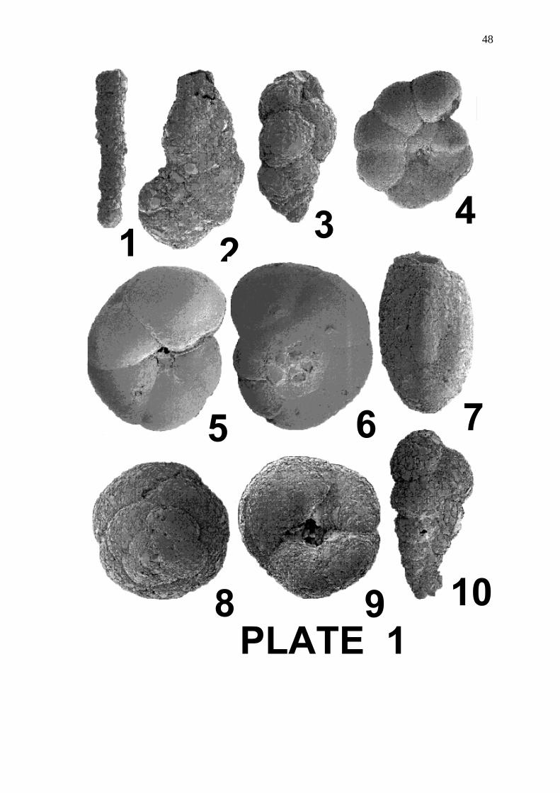
Plate 1

Figure 1: Protoschista findens (Parker) 1870; side view (x130)

Figure 2: Ammotium cassis (Parker) 1870; side view (x 205)

Figure 3: Eggerella australis (Collins) 1958; side view (x 160)

Figure 4: Haplophragmoides canariensis (d'Orbigny) 1839; side view (x 130)

Figures 5, 6: Trochammina inflata (Montagu) 1808, ventral (x 160) and dorsal (x 190)

views of different individuals

Figure 7: Miliammina fusca Brady, 1870; side view (x 200)

Figures 8, 9: Tritaxis conica (Parker and Jones) 1865; dorsal (x 225) and ventral (x 270)

views of different individuals

Figure 10: Textularia earlandi Parker 1952; side view (x 300)

50

21 3

5

7

6

PLATE 28

4

9

51

Plate 2

Figures 1, 2: Quinqueloculina seminula (Linnaeus) 1767; opposite views (x 150) of

different individuals

Figure 3: Brizalina striatula (Cushman) 1922; side view (x 195)

Figures 4, 7: Ammonia aoteana (Finlay) 1940: dorsal (x 170) and ventral (x 150) views of

different individuals

Figures 5, 8: Guttulina problema (d'Orbigny) 1826; side views (x 115, x 110) of different

individuals

Figure 6: Elphidium depressulum (Cushman) 1933; side view (x 140)

Figure 9: Elphidium lene Cushman and McCulloch,1940; side view (x 135) (after Albani

et al., 2001)