controltheory,tsrt09, tsrt06 … · • starred (∗) exercises deals with discrete-time systems...
TRANSCRIPT

CONTROL THEORY, TSRT09,
TSRT06
Exercises & solutions
16 november 2016


Reading instructions
• The names and numbers of the chapters in this exercise collection areconsistent with the names and numbers of the chapters in the textbook.
• Starred (∗) exercises deals with discrete-time systems and are optional.


1 Introduction
1.1
Consider the linear feedback control system given by the figure below.
Σ G(s)
−F (s)
Show that if the small gain theorem (Swe: lagforstarkningssatsen) is fulfilledthe Nyquist criterion is also fulfilled.
1.2
Consider a static nonlinear system described by an ideal relay given by thefunction
y(t) = f(u(t)) =
1, u > 00, u = 0−1, u < 0
.
What is the gain of the relay?
1

1.3
Consider the system
Y (s) = G(s)U(s) G(s) =2
s2 + 2s+ 2
The control signal goes through a valve with saturation
u(t) =
1, if u(t) > 212u(t), if |u(t)| ≤ 2
−1, if u(t) < −2
The output is thus
y(t) = G(p)u(t).
The system is controlled using proportional feedback, i.e. u(t) = −Ky(t). Forwhat values of K is the closed-loop system guaranteed to be stable accordingto the small gain theorem?
1.4
Compute the norms ‖ · ‖∞ and ‖ · ‖2 of the continuous-time signals
(a)
y(t) =
a sin(t), t > 00, t ≤ 0
(b)
y(t) =
1t, t > 1
0, t ≤ 1
(c)
y(t) =
e−t(1− e−t), t > 00, t ≤ 0
.
2

1.5
Consider the linear system
G(s) =ω20
s2 + 2ζω0s+ ω20
.
Compute the system gain ‖G‖ for all values of ω0 > 0 and ζ > 0.
1.6
Analyze the stability of the following system, first by using the small gaintheorem and then by computing the poles of the closed-loop system. Explainpossible differences.
K
a
s+ aΣ
1.7
Consider the feedback control system
−f(·)
G(s)Σ
where G(s) is a linear system with the magnitude plot
3

|G(iω)|
ω [rad/s]10
11.5
and f(·) s an amplifier with the following input-output relationship
f(x)
0.5
1 x
Is the closed-loop system stable?
1.8
Consider a DC motor given on state-space form
x1 = x2
x2 = −ax2 + au
y = x1
The inverse time constant a can vary as
a = 1 + ρ, |ρ| < δ.
The system is controlled using a proportional controller u(t) = −Ky(t).Suppose that a is constant. Give a sufficient condition on K such that theclosed-loop system is stable for all a.
4

1.9
Once again consider the DC motor in exercise 1.8, but now assume that theparameter a can vary arbitrarily fast with time
a = a(t) = 1 + ρ(t), |ρ(t)| < δ, ∀t
(a) Introduce a new, artificial input signal w and a new artificial output sig-nal z such that the system can be described by the feedback connectionbelow
G
u
w
y
z
−K
ρ(t)
(b) Consider the time-varying, static system from z(t) to w(t):
w(t) = ρ(t) · z(t), |ρ(t)| < δ, ∀t.
Show that the gain of this system (according to Definition 1.1 in thetextbook) is at most δ.
(c) Give a sufficient condition on K, for instance an inequality that impli-citly characterizes K, for the closed-loop system to be stable no matterhow a(t) varies with time.
5

6

2 Representation of Linear Systems
2.1
A simplified model of an alternating-current generator can be described asfollows. The input signals to the system are the magnetizing current Im,which is fed into the armature winding, and the driving torque M which isapplied to the rotor axis. The rotation speed of the generator is ω, and thechange in rotation speed is given by
Jω = M −Me
whereMe = Ke · ω · If
is the electrical torque due to the emf. If is the current in the stator winding,given by the relationship
e = R · Ifwhere the voltage e is generated in the stator winding according to
e = Ce · Im · ω
and R is the load resistance applied to the stator winding. Consider e and ωas output signals, M, Im and R as input signals. Set Ke = Ce = J = 1 andfind a state-space representation for this sytem.
Linearize around the stationary point
ω0 = R0 = Im0 = M0 = 1
and derive the transfer function matrix from
u =
∆M∆Im∆R
to y =
[∆ω∆e
]
7

2.2
Consider the system consisting of two coupled tanks described in the figurebelow.
h1h2
u1 u2
y
The flow of water into the left and right halves of the tank are denoted u1
and u2 respectively. These flows are the input signals. The water levels in thetwo halves are denoted h1 and h2 respectively. The flow y out from the tankis assumed to be proportional to the water level in the right half of the tank
y(t) = αh2(t)
The flow between the two halves is proportional to the difference betweenthe levels
f(t) = β(h1(t)− h2(t))
where a flow from left to right is considered positive. Let hi, ui and y bedeviations from nominal values. Thus, they can have negative values. Assumethat the area of the halves are A1 = A2 = 1.
(a) Derive the transfer function from u1, u2 to y.
(b) Compute the maximum and minimum singular values of G(0) and givean intuitive explanation to the corresponding input signals.
8

2.3
Find a state-space realization of the system
G(s) =[
1(s+1)(s+2)
s+3(s+1)(s2+s+1)
]
2.4
Find a state-space realization of the system
y(t) =p
p2 + 4p+ 4u1(t) +
p− 1
p2 + 5p+ 6u2(t)
2.5
A system is described by the differential equation
y + a1y + a2y = b11u1 + b12u1 + b21u2 + b22u2.
Find a state-space realization.
2.6
Consider the system
y1 + y2 = u+ 2u
y2 + y2 + y1 = u
Find a state-space realization.
9

10

3 Properties of Linear Systems
3.1
Consider the transfer function matrix
G(s) =
( 1s+2
− 1s+2
1s+2
1s+2
s+1s+2
1s+2
)
Derive the pole and the zero polynomials of the system? What is the dimen-sion of a minimal state-space realization?
3.2
Find the poles and zeros of
G(s) =1
(s+ 1)(s+ 3)
(1 0−1 2(s+ 1)2
)
3.3
Find the poles of
G(s) =1
(s+ 1)2
(1− s 1
3− s
2− s 1− s
)
.
What is the dimension of a minimal realization?
3.4
(a) Consider the system
G(s) =
(s+5
s2+3s+21
s+2
1s+4
1s+2
)
What is the dimension of a minimal state-space realization?
11

(b) Consider the system
G(s) =
(s+5
s2+3s+21
s+2
1s+4
1s+4
)
What is the dimension of a minimal state-space realization?
3.5
A system has the following input-output relation
y1 + y1 − y2 = u1 − u2
y2 + y1 + y2 = u1 + u2.
Find a matrix fraction description , y(t) = A(p)−1B(p)u(t), and compute thepoles and zeros of the system.
3.6
Consider the MIMO system:
x(t) =
−2 1 00 −1 00 0 −3
x(t) +
0 11 01 0
u(t)
y(t) =
(1 0 00 1 0
)
x(t)
Find a minimal relization of the system, i.e. a realization that is controllableand observable.
12

3.7
Consider the multivariable system
Y (s) = G(s)U(s)
where
G(s) =
(1
s+13
s+22
s+31
s+4
)
(a) Determine the maximum and minimum singular value of the frequencyreponse at the frequency ω = 2 rad/s.
(b) Determine also the input vectors, in terms of their Fourier transforms,corresponding to the largest and smallest gain of the system at ω = 2.
(c) Generate, in Matlab, an input vector that corresponds to the largestgain of the system and simulate the system using this input.
Hint: Use sinusoidal input signals and use the following properties ofa sinusoidal signal considered over a finite time interval.
– The Fourier transform is proportional to the amplitude of thesinusoidal signal, i.e. for u1(t) = A sinωt the Fourier transformU1(iω) is proportional to A.
– Time delay of a signal corresponds to a change of the argumentof the Fourier transform, i.e. if u1(t) = A sinωt has the transformU1(iω) the signal A sin(ωt+ φ) has the transform U1(iω)e
iφ.
(d) Verify that the obtained output signals correspond to largest gain ofthe system.
3.8
Find the poles and zeros of
G(s) =
( 1s+1
0 s−1(s+1)(s+2)
−1s−1
1s+2
1s+2
)
.
13

14

5 Disturbance Models
5.1
A continuous-time stochastic process u(t) has the power spectrum Φu(ω).For the power spectra below, find linear filters such that the processes canbe represented as white noise fed through those filters.
(a) Φu(ω) =a2
ω2 + a2
(b) Φu(ω) =a2b2
(ω2 + a2)(ω2 + b2)
5.2
A position sensor is mounted on a machine that vibrates with a frequencyaround 5 Hz, and this causes that a disturbance n(t) affects the position mea-surement. In order to include the properties of the measurement disturbancein the control design one formulates a a model that describes the proper-ties of the disturbance as filtered white noise V . The following models aresuggested
(i) N(s) =1
s+ 0.001V (s)
(ii) N(s) =900
s2 + 6s+ 900V (s)
(iii) N(s) =25
s2 + s+ 25V (s)
Which disturbance model is the best choice?
15

5.3
Consider a missile propelled by the thrust u. The missile’s position is z. Asimplified model for the air drag is
f = k1 · z + v
where v are, more or less, random wind gusts.
(a) Derive a state-space representation and an input-output representationfor how the controlled output z depends on u and v.
(b) The system disturbance v has the spectral density
Φv(ω) = k0 ·1
ω2 + a2
Modify the state-space representation in (a) to make it possible toexpress the system disturbance using white noise. What is the corre-sponding transfer function?
5.4
Assume, in exercise 5.3, that the position z is measured with an error
y(t) = z(t) + n(t)
Derive a state-space model for the missile if
(a)Φn(ω) = 0.1
(b)
Φn(ω) = 0.1ω2
ω2 + b2.
(c)
Φn(ω) = 0.11
ω2 + b2.
16

5.5
A system has the state-space representation
x = Ax+Bu+Nw
y = Cx+ n
We assume that the system disturbance w changes stepwise and that themeasurement noise is periodical with a frequency of about 2 Hz.
Modify the state-space representation to make it possible to model the distur-bances.
5.6
In airplanes it is common to measure acceleration as well as speed. Theacceleration is measured using accelerometers and the speed is calculatedfrom measurements of air data, such as dynamical pressure et cetera. Thus,the measurements are independent, but of course they are related to eachother.
(a) Derive a state-space model for the speed and acceleration. Let the me-asured speed and acceleration be output signals and assume that thederivative of the acceleration is white noise. Furthermore, assume thatthe measurement errors in speed and acceleration are white noises, in-dependent of each other.
(b) Discuss how we can get better estimates of the speed and accelerationusing Kalman filtering.
5.7
The depicted dynamical system is described by the differential equation
17

x(t)
v(t)
x(t) + x(t) = v(t)
The external force v(t) is white noise with
E v(t) = 0
E v(t)v(s) = δ(t− s)
We want to estimate the position x(t) and speed x(t) at every time instant.We have sensors for both speed and position but for economical reasons weonly want to use one sensor. We can choose between
Alternative I: The measured signal is
y1(t) = x(t) + e1(t)
Alternative II: The measured signal is
y2(t) = x(t) + e2(t)
The measurement errors are e1(t) and e2(t). For simplicity we assume thatthey are both white noises with
Ee1(t) = Ee2(t) = E[e1(t)e2(s)] = 0
Ee1(t)e1(s) = Ee2(t)e2(s) = δ(t− s)
For each alternative derive the linear filter that, in steady state, yields thebest estimate of x(t) and x(t), in the sense of smallest variance of the esti-mation error, from measurements up to and including time t. State, with anexplaination, which alternative you think is the best.
18

5.8
Consider the depicted radar antenna.
Antenna
Motor
Θ
From noisy measurments of the position of the antennaΘm we want to esti-mate the true position Θ. To be able to do this we need a model of thesystem. To this end, describe the dynamics of the antenna with
JΘ(t) +BΘ(t) = τ(t) + τd(t),
where J is the moment of inertia for the moving parts of the antenna, B isthe coefficient of viscous friction, τ(t) is the torque produced by the motor,and τd(t) is the torque caused by the wind. Assume that τd(t) can be modeledas white noise. Furthermore, assume that the torque τ(t) is proportional tothe motor voltage , µ(t), i.e.
τ(t) = kµ(t)
Finally, let us for simplicity, assume that the measurement error can be mo-deled as additative white noise em(t). Hence, the output signal is
Θm(t) = Θ(t) + em(t).
Discuss how Θ(t) can be estimated from Θm(t) using a Kalman filter.
Technical data:B/J = 4.6 s−1
k/J = 0.787 rad/Vs2
J = 10 kg m2
E τd(t)τd(s) = vdδ(t− s) = 10 N2m2 · δ(t− s)
E em(t)em(s) = vmδ(t− s) = 10−7 rad2 · δ(t− s)
19

5.9
Consider an electric motor with transfer operator
G(p) =1
p(p+ 1)
from input voltage to actual angular displacement. The motor operates intwo disturbance modes:
(i)y(t) = G(p)(u(t) + w(t))
(ii)y(t) = G(p)u(t) + w(t)
In both cases we have w(t) = 1pv(t) where v(t) is a unit disturbance, for
example an impulse.
(a) Realize both cases on state-space form. For case (ii) it is assumed thatthe states caused by the disturbance are separate from the ones descri-bing the motor dynamics.
(b) For both cases, give examples of physical phenomena that can be mo-deled with the disturbance w(t) .
(c) Study the two state-space realizations. Are all states controllable? Canstates corresponding to w(t) be made unobservable? Can the influenceof w(t) on y(t) be eliminated?
5.10
Consider the movement of a swing due to the wind. The swing is descibedby the transfer operator
y(t) =1
p2 + p+ 1u(t)
20

where the output signal y(t) is the angular displacement and the input signalu(t) is the torque about the point of suspension. The influence of the windcan be modeled as
u(t) = Kv(t)
where v(t) is a Gaussian distributed disturbance with the spectrum
Φv(ω) =2α
α2 + ω2, α > 0.
K quantifies the strength of the wind and α quantifies the gustiness of thewind.
(a) Does α increase or decrease when the gustiness increases, i.e. when thewind changes direction more frequently?
(b) Derive and interprete conditions on α and K such that the swing hasan angular displacement of more than 1.15 at least a quarter of thetime. This is equivalent to the output having a variance greater than1.
Hint:
1
2π
∫ ∞
−∞
|b2(iω)2 + b1iω + b0|2|(iω)3 + a2(iω)2 + a1iω + a0|2
dω
=b22a0a1 + (b21 − 2b0b2)a0 + b20a2
2a0(−a0 + a1a2)
21

22

6 The Closed-Loop System
6.1
For a given system G and a given controller F we have defined four transferfunctions as
Gwuu = (I + FG)−1, Gwu = −(I + FG)−1F
Gwuy = (I +GF )−1G, Gwy = (I +GF )−1
All four transfer functions have to be stable for the closed-loop system to beinternally stable.
Show that (Gwuu Gwu
Gwuy Gwy
)
=
(I F
−G I
)−1
6.2
The system
G(s) =s− 1
s+ 1
and the controller
F (s) =s+ 2
s− 1
are are used in the feedback connection depicted below.
Σ G(s)
−F (s)
Compute Gc, T and S. Are they stable? Is the closed-loop system internallystable?
23

24

7 Limitations in Control Design
7.1
Given the system
G(s) =s− 3
s+ 1.
we want the complementary sensitivity function to be
T (s) =5
s+ 5.
(a) Compute a controller Fr = Fy = F which results in this T . Will thiscontroller really work?
(b) Suggest an alternative T , still having the bandwidth 5 rad/s, but re-sulting in an internally stable system with Fr = Fy = F.
(c) A rule of thumb for control of non-minimum phase systems states thatthe bandwidth of the closed-loop system cannot realistically be greaterthan half the value of the non-minimum phase zero. In this case 1.5rad/s. Have we cirumvented this rule of thumb in the above design ordoes the closed-loop system have any disadvantages?
7.2
A continuous-time system has a zero at s = 3 and a time-delay of 1.0 second.What is the upper limit of the realistic bandwith/crossover frequency if themagnitude curve of the open-loop system decreases monotonically?
7.3
Give an example of a system for which there exists no controller having allthree properties: a stable closed-loop system, small magnitude of the sen-sitivity function at low frequencies and small amplification of measurementerrors at high frequencies.
25

7.4
A multivariable system is supposed to attenuate system disturbances (w) atleast a factor 10 for frequencies under 0.1 rad/s. Furthermore, measurementdisturbances (n) should be attenuated at least a factor 10 for frequenciesabove 2 rad/s. Constant system disturbances should be attenuated at leasta factor 100 in steady state.
(a) Formulate conditions on the singular values of S and T which willguarantee that the requirements are fulfilled.
(b) Translate the specifications into requirements on the loop gain GFy.
(c) Formulate the requirements using ‖ · ‖∞ and frequency weights WS ochWT .
(d) Which crossover frequency and phase margin would we expect, havingthe weights i (b), had the system been a SISO system? What lowerbound on ‖T‖∞ does this result in?
(e) Is this lower bound on ‖T‖∞ consistent with the requirements in (c)?
7.5
A control system has the sensitivity function S, depicted below
A1
A20
log |S(iω)|
ω
What can be stated about the open-loop system if the surface A2 is largerthan the surface A1?
26

7.6
For a certain feedback system we demand that:
(i) output disturbances, with frequencies under 2 rad/s, should be attenu-ated at least a factor 1000.
(ii) the system should remain stable despite a model uncertainty
|∆G| ≤ 100|G|
for frequencies above 20 rad/s. G is the frequency response of the no-minal system and ∆G is the absolute error in the frequency response.
Can this be accomplished using a linear, time-invariant controller?
7.7
We have the following specifications on a SISO system
|S(iω)| ≤ 10−3, ω ≤ 1
|T (iω)| ≤ 10−3, ω ≥ 100
(a) State two non-constant frequency weights WS and WT which wouldguarantee that the specifications are met.
(b) Trying to find a controller fulfilling the design criteria, for exampleusing the methods presented in Chapter 10 in the textbook, we fail.Should this have been anticipated from the very beginning?
27

28

8 Controller Structure and Control Design
8.1
Let
G(s) =
(1
s+210s+1
1s+5
5s+3
)
.
(a) Compute RGA(G(0)).
(b) Which input-output pairing should be avoided?
8.2
Given the multivariable system
(y1y2
)
=1
0.1s+ 1
(0.6s+1
−0.4
0.3 0.6
)(u1
u2
)
.
Assume that we want the controller to be diagonal and that we use therelative gain array (RGA) to decide what input should control what output.Furthermore, assume that we want a crossover frequency of ωc = 10 rad/s.Decide how the signals should be paired.
8.3
Study the multivariable system
(y1y2
)
=
(1
10s+1−2
2s+1
110s+1
s−12s+1
)(u1
u2
)
.
(a) Decide, using RGA analysis, which input signal should control whichoutput signal.
29

(b) Assume that we want to use decentralized control, i.e. we want a con-troller on the form
F diag(s) =
(F11(s) 0
0 F22(s)
)
.
Furthermore, assume that we do not want the steady-state error inone channel to affect the steady-state error in the other channel. Gi-ve the structure of a controller F (s), expressed in F diag(s), that willaccomplish this.
8.4
Design a controller, using the IMC method, for a stable first order process
G(s) =K
τs+ 1, τ > 0.
What type of controller do we get? Compute the sensitivity function and thecomplementary sensitivity function and sketch the Bode plot of the sensitivityfunction. What does Bode’s integral theorem state for this case?
8.5
Design a controller, using the IMC method, for the system
G(s) =6− 3s
s2 + 5s+ 6.
What type of controller do we get?
8.6
Consider the DC motor
y =1
p(p+ 1)u
30

Compute an IMC based controller for this system. Write the controller onthe form u = −Fy(p)y, and sketch the Bode plot for Fy(p). Approximatelywhat type of controller do we get when we want a high bandwidth for theclosed-loop system?
8.7
Given the multivariable system
G(s) =1
s/20 + 1
(9
s+12
6 4
)
.
(a) What are the poles and zeros of G(s)?
(b) Compute an IMC based controller for the system.
8.8
Consider the system
G(s) =
2s+1
3s+2
1s+1
1s+1
(Example 1.1 in the textbook)
Show how an IMC based controller can be computed for this system. Givean explicit expression for the corresponding sensitivity function.
8.9
Consider the multivariable system
Y (s) = G(s)U(s)
31

where
G(s) =
2
s+ 1
3
s+ 2
α
s+ 1
1
s+ 1
and α > 0.
(a) Determine the zero of the multivariable system. How does the zerodepend on the value of α?
(b) Assume that one would like to achive complete decouple of the systemG(s) such that
G(s)F (s) =
1
(s+ 1)20
01
(s+ 1)2
Are there any cases when this is not a good idea? Motivate!
(c) Assume that one instead chooses to use a static decoupling such thatG(s)F (s) is decoupled for ω = 0. Are there any values of α for whichthis is not a good idea? Motivate!
8.10
Consider the multivariable system
Y (s) = G(s)U(s)
where
G(s) =
1
s+ 2
2
s+ 4
1
s+ 1
1
s+ 2
(a) Determine the RGA at ω = 0.
32

(b) Assume that the system is going to be controlled by a diagonal regulator
U(s) = F (s)(R(s)− Y (s))
where
F (s) =
(K 00 K
)
Use the result from a) the judge how successful this will be. Determinealso the poles of the closed loop system for the case K = 5.
(c) How can the problem be modified such that a diagnonal F (s) can beused? Verify that the closed loop system is stable for K = 5 for themodified problem.
33

34

9 Minimization of Quadratic Criteria: LQG
9.1
Consider the system
G(s) =1
s− 1
represented on state-space form with noise as
x(t) = x(t) + u(t) + v1(t)
z(t) = x(t)
y(t) = x(t) + v2(t)
The noises vi(t) are white with intensities Ri. We use the criterion
V =
∫
Q1x2(t) +Q2u
2(t) dt,
and want to find the LQG controller.
(a) Show that the controller is a function of α = Q1/Q2 and β = R1/R2
only.
(b) Compute the poles of the closed-loop system as a function of α and β.
9.2
Consider the system
z =1
p+ 1u+
1
p+ 1v
y = z + e
where v and e are unit disturbances with spectra
Φv(ω) ≡ r1 respektive Φe(ω) ≡ 1.
We minimize the criterion
V =
∫
q1z2(t) + u2(t) dt
35

(a) Compute the loop gain of the feedback connection.
(b) How do r1 and q1 influence the loop gain?
(c) Sketch the magnitude of the frequency response. What happens whenr1 → ∞ and when q1 → ∞ respectively?
9.3
Consider the double integrator
z(t) = u(t).
We want to find a controller such that the criterion∫ ∞
0
(z2(t) + η · u2(t)) dt
is minimized for some η > 0. We assume that z(t) and z(t) are both measured.
Where are the poles of the optimal closed-loop system located? How is thecontrol signal affected when η is decreased?
9.4
Consider the antenna in Exercise 5.8. We want to control it and a suitablemeasure on the performance of closed-loop system is given by the criterion
J = EΘ2(t) + ρµ2(t)
where ρ is a constant we can choose. Derive an optimal control signal anddiscuss how it is to be combined with the Kalman filter.
9.5
Consider control of the DC motor
G(s) =1
s(s+ 1)
36

We want to use the motor together with a system that has a resonancepeak at approximately 0.5 rad/s. Other than that, we do not know muchabout the system. Describe how we can compute an LQG controller withgood robustness qualities, i.e. small complementary sensitivity gain, at thisfrequency.
9.6
A system has static gain G0. It is influenced by system disturbances, withall energy concentrated at zero frequency, i.e.
Φν(ω) = δ(ω)
The reference signal is zero, as is the measurement noise. We choose a con-troller that minimizes
Ey2(t) + αu2(t)
What is the value of the sensitivity function at zero frequency?
9.7
Consider the system
z =1
p + 1u+
1
p+ 1ν
y = z + e
where ν is noise of very low frequency,
ν =1
p+ εv,
v and e are noises with Φv(ω) ≡ Φe(ω) ≡ 1.
(a) Find a controller that minimizes
Ez2 + u2
when ε → 0.
What is the static gain of the sensitivity function?
37

(b) Use output-LTR (LTR(y)) to compute L. What is the static gain ofthe sensitivity function?
9.8
Consider a motor driving two rotating masses connected by a flexible shaft:
Motor
ϕ1 ϕ2
The angular displacements of the masses are ϕ1 and ϕ2 respectively and ω1
and ω2 are the angular velocities. The moments of inertia are 10 for bothmasses. The spring rate of the shaft is k and the damping factor is 0.1. Theinput is the voltage applied to the motor. With the states x1 = ϕ1 − ϕ2,x2 = ω1 and x3 = ω2 we get the state-space representation
x =
0 1 −1
−12ω20 −0.01 0.01
12ω20 0.01 −0.01
x+
0
ω0
0
u
z =(0 0 1
)x
where
ω20 =
k
50
The Bode plot, when k = 1, is shown in the figure below. There is a resonancepeak at the frequency ω0. The spring rate is not exactly known, but has avalue close to 1. We want to design a controller that yields a stable closed-loopsystem despite variations in k.
How can the above model be extended with a model for the noise to assurerobustness for an uncertain value of k when we use LQG controller design?Give an actual example of such an extended system.
38

10-2
10-1
100
10-3
10-2
10-1
100
101
ω rad/s
|G(iω)|
9.9
Consider the system
x(t) =
(1 00 −2
)
x(t) +
(32
)
u(t)
Show thatu(t) = −
(2 −3
)x(t)
cannot be an optimal state feedback for any quadratic criterion on the form
min
∫
(xT (t)Q1x(t) +Q2u2(t)) dt
where Q1 is a positive definite matrix.
9.10
Consider the system
x =
(1 −12 4
)
x+
(−48
)
u
y = (1 1) x
39

We want to minimize the criterion
V (T ) =
∫ T
0
xT (t)x(t) + u2(t)dt
Is it possible to find a state feedback u = −Lx such that V (T ) < ∞ whenT → ∞?
9.11
The figure below shows a simple electrical circuit.
u [V]R L
C
i [A]VC [V]
Introduce the state variables x1 = VC and x2 = i. With the component values
R = 5 Ω, L = 0.1 H, C = 1000 µF
we get the state-space representation
x(t) =
(0 1000
−10 −50
)
x(t) +
(010
)
u(t)
y(t) =(1 0
)x(t)
Compute a state feedback that minimizes
J =
∫ ∞
0
(x22(t) + 0.01u2(t)
)dt
This criterion aims at limiting the power loss without getting too large sig-nals.
40

9.12
A system has the state-space representation
x(t) =
−2 −1 11 0 0.50 0 A
x(t) +
10.50
u(t) +
001
v(t)
z(t) =(1 0 0
)x(t)
y(t) = z(t) + e(t)
where e(t) are v(t) ar unit disturbances.
The controller, a feedback from reconstructed states, minimizes
E[z2(t) + u2(t)
]
How does the value of A affect the sensitivity function?
9.13
A simplified model for how the elevator angle affects the movements of anairplane is given by
x =
−0.01 0.03 −100 −1 3000 0 −0.5
x+
4−20−10
u
where
x =
roll angleyaw anglepitch-angle velocity
In particular we are interested in the control of the pitch-angle velocity andchoose the controlled variable to be
z =[0 0 1
]x
All state variables are measured
y = x+ e
41

We want to design a feedback from reconstructed states using LQG metho-dology. It is especially important that the sensitivity function has a smallgain for frequencies around 1 rad/s. Show how to modify the model of theairplane to achieve such a sensitivity function.
9.14
Consider the system
x(t) = αx(t) + u(t) x(0) = x0 (1)
The system is controlled by the feedback
u(t) = −Lx(t) (2)
where L is chosen such that
J =
∫ ∞
0
x2(t) + ρu2(t))dt (3)
is minimized.
(a) Determine L as function of ρ and α.
(b) If it is desired to keep u(t) small, this can be achieved by choosing ρlarge. What is the resulting L when ρ → ∞? Consider, for example,the cases α = 1 and α = −1, respectively. Why is it not optimal tochoose L = 0, i.e. u(t) = 0, in both cases?
9.15
An electrical motor has the transfer functions
Y (s) =1
s(s+ 1)U(s)
and it is controlled using state feedback
u(t) = −Lx(t) (r(t) = 0)
42

where x1(t) = y(t) and x2(t) = y(t). The gain vector L is determined byminimizing the criterion
J =
∫ ∞
0
xT (t)Q1x(t) +Q2u2(t)dt
Figure 1 shows the simulation results when the system starts in the initialcondition x(0) = (1 1)T for some different choices of Q1 and Q2. Combinethe figures with the choices of matrices.
(i)
Q1 =
(1 00 0
)
Q2 = 0.1
(ii)
Q1 =
(1 00 10
)
Q2 = 1
(iii)
Q1 =
(0.1 00 0
)
Q2 = 0.1
(iv)
Q1 =
(1 00 0
)
Q2 = 1
43

0 5 10−0.5
0
0.5
1
1.5A
0 5 10−1
−0.5
0
0.5
1
1.5B
0 5 10−0.5
0
0.5
1
1.5C
0 5 10−0.5
0
0.5
1
1.5D
Figur 1:
9.16
Consider the simplified description of an aircraft in the figure below.
α
θ
v
δ
h
Using the state space variables
44

x1(t) = α(t) angle of attack (rad)
x2(t) = θ(t) pitch rate (rad/s)x3(t) = θ(t) pitch angle (rad)x4(t) = h(t) height (deviation from an operating point)
the input signal
u(t) = δ(t) control surface angle (rad)
and output signal
y(t) = h(t) height (hundreds of meters)
the system is decribed by the state space model
x = Ax+Bu y = Cx
where
A =
−0.17 1 0 0−0.56 0 0 0
0 1 0 0−2.22 0 2.22 0
, B =
0.0110.5600
, C = (0 0 0 1).
(a) Is the system asymptotically stable?
(b) Assume that the system has the initial state
x0 = (0 0 0.1 1)T
and that the system is controlled by the state feedback
u = −Lx
where the gain vector L is chosen such that the criterion∫ ∞
0
xT (t)Q1x(t) + uT (t)Q2u(t) dt
is minimized. Assume that the matrices are chosen as
Q1 =
0 0 0 00 0 0 00 0 0 00 0 0 1
, Q2 = 1
Determine the poles of the closed loop system. Simulate the closed loopsystem.
45

(c) Assume that Q2 is varied. How does that affect the location of theclosed loop poles and the properties of x and u?
(d) Assume now that the following conditions shall be fulfilled:
– |x1| < 0.2 all the time.
– |x4| < 0.1 after 25 seconds.
– |u| < 0.5 after one second.
Determine Q1 and Q2 such that these conditions are satisfied. What isthe resulting location of the closed loop poles?
9.17
The figure below illustrates a system consisting of a ball on a plane. Thevariable r denotes the position of the ball relative to the center of the plane,and α represents the angle of the plane. The input signal is the torque thatrotates the plane.
α
r
Figur 2: Ball on plane.
The system is represented by the state variables
x1(t) - position, r(t)x2(t) - velocity, r(t)x3(t) - plane angle, α(t)x4(t) - plane angular velocity, α(t)
and torque is the input signal u(t). The state space model is
x(t) = Ax(t) +Bu(t)
46

where
A =
0 1 0 00 0 −7 00 0 0 10 0 0 0
B =
0001
C =(1 0 0 0
)
(a) Assume that the system starts in the initial state
x(0) = (0.1 0 − 0.1 0)T
i.e. the ball is positioned to the right of the center, and the plane leansdownwards on the right side. Assume that all state variables can bemeasured. Determine a state feedback such that the following require-ments are fulfilled:
– | x(t) |→ 0 when t → ∞.
– | x1(t) |≤ 0.2 ∀ t.
– | u(t) |≤ 2.5 ∀ t
Determine also the absolute value of the poles of the closed loop system.
(b) Verify that all sensors that measure the states have to work in order toobtain a stable closed loop system.
Hint: The characteristic equation of the closed loop system is given by
λ4 + l4λ3 + l3λ
2 − 7l2λ− 7l1 = 0
Missing a sensor is equivalent to setting the corresponding feedback lito zero.
47

48

10 Loop Shaping
10.1
Consider the system
y =1
p+ 1u
We want to create a closed-loop system with S, T and Gwu, such that∫ ∣∣∣∣
S(iω)
iω
∣∣∣∣
2
+ |0.5 T (iω)|2 + |5Gwu(iω)|2 dω
is minimized. Compute the controller.
10.2
Consider the system
y =1
p+ 1u
We want to create a closed-loop system with S, T and Gwu, such that
|S(iω)| < γω
|T (iω)| < 2γ
|Gwu(iω)| < 0.2γ
Write down the equations that determines the controller.
10.3
Consider the SISO system G(s) with state-space realization
x = Ax+Bu
y = Cx
We want to use loop shaping with the weights
WS =1
s, WT = 1, Wu = 1
49

(a) State the equations that determine the optimal controller in H2 andH∞ respectively.
(b) Explicitly write down the observer for the extended state vector andshow that the optimal controller can be written as
u(t) =α
1 + L(pI − A)−1B
∫ t
0
y(τ) dτ
for some L, where α = 1 for the H2 controller and α > 1 for the H∞controller. State the equation determining L.
(c) Show that the controller will have a pole at the origin unless the systemdoes itself has a pole at the origin.
10.4
Once again consider the system in Exercise 9.8.
(a) Suggest frequency weights WS, WT and Wu, for H2 and H∞ design,such that we get robustness against uncertain values of k.
(b) State the extended system from u and w to z on state-space form.
10.5
A DC-motor has transfer function
G(s) =1
s(s+ 1)
and it going to be controlled using proportional feedback
U(s) = K(R(s)− Y (s))
The properties of the closed loop system is specified via the requirement
| S(iω) |<| W−1S (iω) | ∀ ω
The figure below shows three alternatives for the weight function W−1S (iω).
Which alternative is the best? Motivate the answer.
50

10−2
10−1
100
101
10−1
100
101
A
10−2
10−1
100
101
10−1
100
101
B
10−2
10−1
100
101
10−1
100
101
C
Figur 3: Suggestions for | W−1S (iω) |.
10.6
The system
Y (s) =1
s+ 1U(s)
is going to be controlled by the proportional feedback
U(s) = K(R(s)− Y (s))
(a) Derive S(s), T (s) and Gru(s) respectively, i.e. the sensitivity function,the complementary sensitivity function and the transfer function fromreference to input signal.
(b) The properties of the control system are specified using the weightfunction according to
| S(iω)WS(iω) |< 1 ∀ω
| T (iω)WT (iω) |< 1 ∀ω| Gru(iω)Wu(iω) |< 1 ∀ω
51

The figures below show three suggestions for weight functions WS,WT
and WU . Two of the alternatives are unrealistically or incorrectly spe-cified. Which are the two incorrect alternatives? Motivate the answer.
(c) Consider the alternative in b) that is realistically specified. Is it possibleto choose K such that all requirements are fulfilled?
101
102
10−2
100
102
10−1
100
101
1/WS
10−1
100
10−1
100
1/WT
10−2
100
102
100
101
102
1/WU
Figur 4: Alternative I
52

102
10−2
100
102
10−1
100
101
1/WS
10−2
100
10−1
100
101
1/WT
10−2
100
102
100
101
102
1/WU
Figur 5: Alternative II
10−2
100
102
10−1
100
101
1/WT
10−2
100
102
100
101
102
1/WU
10−1
100
101
102
10−1
100
1/WS
Figur 6: Alternative III
53

54

12 Stability of Nonlinear Systems
12.1
Given the nonlinear differential equation
y + 0.2(1 + y2)y + y = 0
let the state variables be x1 = y and x2 = y. Try to show that the origin isa stable equilibrium by using the Lyapunov function candidate
V =1
2(x2
1 + x22).
12.2
Consider the system
x1 = sin x1 + x32
x2 = x1 − x2
Is it possible to use the function
V (x1, x2) = −1
2x21 +
1
4x42
to prove Lyapunov stability for the above system? Motivate your answer.
12.3
A nonlinear function lies in the sector
55

Slope 3
Slope 0.5
According to the circle criterion, what circle in the complex plane correspondsto this nonlinearity?
12.4
A nonlinear system is described by the following block diagram
Σr
G(s)
f−1
where G(s) is a linear system and the static nonlinearity f is given in thefigure below (the saturations at −1 and 1 extends to −∞ and ∞).
56
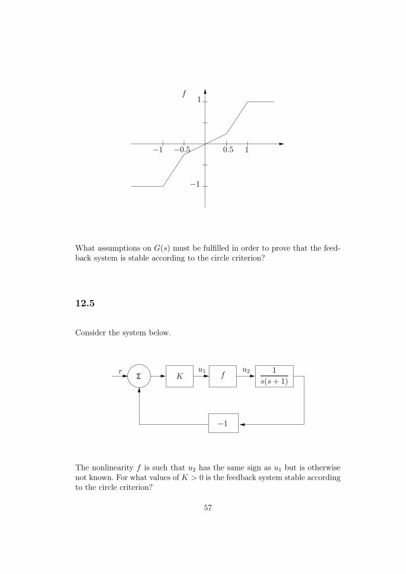
1
1
−1
−1
−0.5 0.5
f
What assumptions on G(s) must be fulfilled in order to prove that the feed-back system is stable according to the circle criterion?
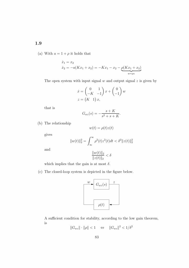
12.5
Consider the system below.
Σr
K f
−1
u1 u2 1
s(s+ 1)
The nonlinearity f is such that u2 has the same sign as u1 but is otherwisenot known. For what values of K > 0 is the feedback system stable accordingto the circle criterion?
57

12.6
Consider the swing depicted below.
Center of gravity
ℓ
Φ
The movement of the swing is described by the equation
Jd2Φ
dt2+mgℓ sinΦ = 0
where m is the mass and J is the moment of inertia. The swing can becontrolled by alternating between bending and stretching the knees whilestanding on the swing. The control signal is the location of the center ofgravity ℓ. We assume that J is constant.
Show that the control signal
ℓ = ℓ0 + εΦΦ, ε > 0
will bring the swing to rest in Φ = 0.
12.7
The block diagram below is given.
58

Σ
Σr = 0
Relay
G(s)
a
b H(s)
−1
−1
1
We have that
H(s) = s and G(s) =1
(s+ 1)(s+ 2).
How shall the feedback coefficients a and b be chosen to guarantee Lyapunovstability?
Hint: Use a quadratic Lyapunov function candidate.
12.8
A servo system contains a nonlinearity where the relationship between theinput signal u and the output signal y is
y = u+ arctan(u)
What requirements on the linear part of the servo system must be fulfilledin order to prove stability using the circle criterion?
59

12.9
A simplified model for the movements of an airplane is given by
x =
−0.01 0.03 −100 −1 3000 0 −0.5
x+
4−20−10
u
All states are measured and the control signal is
u = −Lx+ r
where L is the feedback that minimizes∫
(xT (t)Q1x(t) + u2(t)) dt
for Q1 = 10 · I
The requested control signal u is different from the actual u, due to thehydraulic servo dynamics. The relationship between u and u is
u
u1 2
0.75
2.5
Will the closed-loop system be stable? Motivate your answer.
60

13 Phase Plane Analysis
13.1
Given the differential equation
y − (0.1− 10
3y2)y + y + y2 = 0
Find and classify the singular points.
13.2
Draw the phase portrait of the depicted position servo.
Σ
−1 a−a
K
s(s+B)
The position is measured using an E-transformer, which can be described asa dead zone. Assume that K > B2
4.
13.3
The following system is given
61

Σ
Relay
−1
−1
1 1
s2
(a) With zero input signal the output of the relay is +1 or −1, dependingon the history of the input signal. The relay does not switch until theinput signal has changed polarity.
Draw a phase portrait of the system.
(b) Due to imperfections the actual feedback loop is
a−a −1
Draw the phase portrait of this system.
13.4
Linus is on his way home after an exam. On the highway outside of Linkopinga gust of wind makes the car drift from the desired path. Your task is to, usingphase plane analysis, decide how the movement of the car will progress. Willit return to the desired path? If the car has a constant speed in the directionof travel the system can be described by the following block diagram
62

Σu y
1s
1s
−G(s)
−1
1
The torque applied to the steering wheel is u. The backlash comes from a gearunit in the steering. The output signal y is the deviation from the desiredpath. G(s) is the transfer function from Linus’ visual perception to the torquehe applies to the steering wheel.
Distinguish between the cases:
(a) G(s) = 1 (there was a party after the exam)
(b) G(s) = 1 + s (there was not a party after the exam)
13.5
A simple ecological system consists of two species of fish. The first kind eatsalgae and the second kind eats the first kind. Let x1 denote the number ofalgae eating fish and x2 denote the number of predatory fish. Then we have
x1 = 2x1 −x1x2
1 + 16x1
− 0.2x21
x2 = −3x2 +x1x2
1 + 16x1
(a) From these equations, calculate the stationary points.
63

(b) Classify the stationary points and sketch the phase portraits in a sur-rounding of them. It is sufficient to consider a linearised version of theequations.
(c) Without any further calculations, merge the phase portraits you havemade around the stationary points in a fashion that seems reasonable.Only consider x1 > x2 > 0.
An interpretation of the given equations is:
If the algae eating fish have an infinite amount of food and lack enemies,their number will grow exponentially as
x1 = 2x1
As there is a limited amount of algae the growth saturates according to
x1 = 2x1 − 0.2x21.
If there are predatory fish x2 present the algae eaters will be devoured at therate
x1x2
1 + 16x1
The interpretation of this term is that if x1 is large every predatory fish caneat until it is full. This corresponds to 6 algae eating fish per time unit. Onthe other hand, if the number x1 is relatively small the predatory fish willeat less.
The second equation says that if the supply of food is unlimited (x1 = ∞)the predatory fish will multiply according to
x2 = 3x2.
If food is lacking (x1 = 0) the predatory fish will expire as
x2 = −3x2
13.6
A mass is suspended from a spring. Its position y(t) satisfies the differentialequation
y(t) + y(t) = f(t)
64

where f(t) is an external force acting on the mass. Draw a phase portrait ofthe system when
f(t) =
−1 if y(t) > 0+1 if y(t) < 0
Will the system reach an equilibrium?
13.7
Consider the system
x =
(−x3
1 + ux1
)
(a) Sketch a phase portrait when u = 0.
(b) Use the Lyapunov function
V (x) = x21 + x2
2
to compute a control signal
u = f(x1, x2)
which will make the origin globally asymptotically stable. Sketch aphase portrait, in a neighborhood of the origin, for the closed-loopsystem.
65

66

14 Oscillations and Describing Functions
14.1
Consider the feedback control system including an input saturation accordingto the figure below.
u 10
s(s+ 1)2
−1
1
1
Σ
(a) Investigate the stability of the system. If a periodical solution exists,determine its frequency and amplitude.
(b) Build a simulation model of the control system and investigate thevalidity of the results from a).
14.2
A temperature control system, depicted below, contains a relay with deadzone.
r(t) = 0 u(t) y(t)
−1
G0(s)Σ
67

G0(s) = 1s(1+s)2
, ±D is the width of the dead zone and ±H is the outputlevel of the relay. The values of the dead zone and output level are such thata stable oscillation just barely can exist. If H is increased or if D is decreasedan oscillation will not be possible.The amplitude of the oscillation is 2.5 units.Compute D, H and the frequency of the oscillation. The describing functionfor a relay with dead zone is
ReYN(C) =4H
πC
√
1−D2/C2, C ≥ D
ImYN(C) ≡ 0
14.3
A relay servo is given by
θref u θ
−L(s)
K
s(s+ 1)2Σ
The gain K is strictly positive.
(a) The feedback used is L(s) = 1. Show that there is an oscillation for allvalues of K.
(b) To avoid too much wear on the system we do not want the amplitudeof the oscillation in θ to be greater than 0.1. For what values of K isthis fulfilled?
(c) We want to use a gainK that is larger than what is possible in (b). Statea feedback L(s) with L(0) = 1 that makes this feasible. No details arenecessary. Just motivate why the feedback should solve the problem.
68

14.4
Consider the nonlinear system
u y
−H(s)
1
s(s+ 1)(s+ 2)Σ
(a) If proportional control is used, i.e. H(s) = 1, a stable oscillation occurs.Find the amplitude and frequency of the oscillation.
(b) To eliminate the oscillation we use proportional and derivative con-trol, i.e. H(s) = 1 +Ks. Show how K can be chosen to eliminate theoscillation.
14.5
Consider the feedback control system where a motor is controlled using arelay with hysteresis.
θr = 0 u(t) θ
−1
1
s(s+ 1)Σ
1
−10.5−0.5
(a) Investigate the stability of the system using the describing functionmethod. If a periodical solution exists, determine its frequency andamplitude.
69

(b) Build a simulation model of the control system and investigate thevalidity of the results from a).
(c) Introduce suitable state variables and sketch a phase portrait.
14.6
Consider the following servo system
r = 0 e u u yΣ
−1
1
s2K(1 + 1
TIs+ TDs)
PID controller amplifier motor
The PID controller has K = 2, TI = 2 and TD = 0.5.
(a) The tuning of the controller was done assuming that the amplifier hasthe transfer function 1. Show that, if this assumption is true, this resultsin an asymptotically stable closed-loop system.
(b) The actual amplifier contains a saturation
−1
−1
1
1 u
u
70

State the amplitude, frequency and stability properties of possible oscil-lations.
(c) Discuss, based on the results from (b), under what circumstances theservo system will function as intended. Especially investigate the influ-ence of different signal amplitudes.
14.7
Consider the feedback control system
Σ
-1
ur(t)=0 y(t)G (s)0
When the system is simulated a limit cycle occurs. Determine the amplitudeand frequency of the limit cycle. The Bode diagram for the linear part GO(s)of the control system is given in the figure below.
0
90
-90
-180
.1 2 5 1 2 5 1
G
Radianer/s0
20
-20
-40
20log|G| dB|G|
1
2
5
10
20
0.5
0.2
0.1
0.05
0.02
0.01
|G |
arg G
0
0
The describing function of a relay with deadzone is given by
Yf(C) =4
πC
√
1− 1/C2 C ≥ 1
71

72

17 To Compensate Exactly for Nonlinearities
17.1
Find a feedback which makes the system
x1 = −x1 + 7x2
x2 = −x2 + cosx1 + u
linear.
17.2
Find an output feedback, u = f(y), which makes the system
x1 = x3 + 8x2
x2 = −x2 + x3
x3 = −x3 + x41 − x2
1 + u
y = x1
linear.
17.3
Find a feedback which makes the system
x1 = x21 + x2
x2 = u
y = x1
linear.
73

17.4
Consider the two tank system:
u
x1
x2
The dynamics of the system is described by
x1 = 1 + u−√1 + x1
x2 =√1 + x1 −
√1 + x2
Which state should be chosen as output to achieve a strong relative degree2? Do a feedback linearization of the system.
17.5
A mass m is suspended from a spring:
m
F
y
74

The force F is generated by the control signal u fed through an actuator suchthat
F =1
s+ 1u
The position of the mass is y. The spring rate and the viscous damping arenonlinear. Thus the force is
−k(y)− d(y).
(a) Realize this system on state-space form. The input signal is u and theoutput signal is y.
(b) Can the system in (a) be made linear using feedback? If so, computesuch a feedback.
75

76

Solutions
77

78

1 Introduction
1.1
The small gain theorem for linear systems can be stated as follows: Assumethat both G(s) and F (s) are stable transfer functions, and interconnectedaccording to the figure below.
Σ G(s)
−F (s)
Then the closed-loop system is stable if
|G(iω)| · |F (iω)| < 1, ∀ω.
The transfer function of the closed-loop system is
Gc(s) =G(s)
1 +G(s)F (s)
Gc(s) is stable according to the Nyquist criterion if the Nyquist curve forG(iω)F (iω) does not encircle the point −1. Since we know from the smallgain theorem that
|G(iω)F (iω)| ≤ |G(iω)| · |F (iω)| < 1,
the Nyquist curve can not encircle the point −1, and hence the Nyquistcriterion is fulfilled.
Note that input-output stability follows from asymptotic stability. Input-output stability is the concept used in the general small gain theorem.
79

1.2
We have that y(t) = f(u(t)) where f(·) is the function describing the idealrelay. The gain is defined as
‖f‖ = supu 6=0
‖y‖2‖u‖2
We have that |f(u)| ≡ 1, ∀u(t) 6= 0, and this yields
‖y‖22 =∫ ∞
−∞y2(t)dt = lim
T→∞
∫ T
−T
[f(u(t))]2dt = limT→∞
2T = ∞
for all choices of u(t) 6= 0 such that 0 < ‖u‖2 < ∞. Take for exampleu(t) = 1
t. This means that an ideal relay has infinite gain.
1.3
f(u) G(s)u
Σ
−K
S1
︷ ︸︸ ︷
︸ ︷︷ ︸
S2
The system is stable according to the small gain theorem if ‖S1‖ · ‖S2‖ < 1.
We have that:
‖S1‖ ≤ ‖f(u)‖ · ‖G‖‖S2‖ = |K|
where
‖G‖ = supω
|G(iω)| = supω
2√
(2− ω2)2 + 4ω2= 1 (for ω = 0)
80

‖f(u)‖2 = ‖u‖22‖u‖22
=
∫∞−∞(f(u(t))2dt
‖u‖22≤[
|f(u(t))| ≤ 1
2|u(t)|
]
≤14‖u‖22‖u‖22
=1
4⇒ ‖f(u)‖ ≤ 1
2
‖S1‖ · ‖S2‖ ≤ 1
2· |K| < 1
i.e. , we must choose |K| < 2 to be able to guarantee input-output stability.
1.4
(a) ‖y‖∞ = |a|, ‖y‖2 = ∞
(b) ‖y‖∞ = 1, ‖y‖2 = 1
(c) ‖y‖∞ =1
4, ‖y‖2 =
1
6
√3
1.5
The gain of the system is
‖G‖ = supω
|G(iω)| = supω
ω20
√
(ω20 − ω2)2 + 4ζ2ω2
0ω2
By differentiating |G(iω)| we see that the magnitude of G(iω) has its maxi-mum at ω = 0 if ζ > 1√
2. This results in the gain
‖G‖ = 1
If 0 < ζ < 1√2the maximum of |G(iω)| is attained at ω = ω0
√
1− 2ζ2. Thisresults in the gain
‖G‖ =1
2ζ√
1− ζ2
81

1.6
One has to distinguish between the cases a > 0 and a < 0 respectively.
(i) For a > 0 the system G(s) is stable and the small gain theorem isapplicable. The system G(s) has gain one, and the small gain theoremhence gives the condition | K |< 1. The characteristic equation of theclosed loop system is given by (Note: positive feedback)
(s+ a)−Ka = 0
which imples the pole s = (K − 1)a, which is located in the left halfplane for K < 1.
(ii) For a < 0 the system G(s) is not stable and the small gain theoremis not applicable. The pole s = (K − 1)a is in the left half plane forK > 1.
1.7
The linear part, represented by G(s), has gain 1.5 according to the figure.For the nonlinear part we assume that f(x) is an odd function, such thatf(−x) = −f(x). The nonlinearity can hence be bounded by
| f(x) |≤ 0.5 | x |and hence the gain is 0.5. Since 1.5 · 0.5 < 1 the closed loop system is stableaccording to the small gain theorem.
1.8
Using proportional control u = −Ky = −Kx1 we get
x1 = x2
x2 = −aKx1 − ax2
The characteristic equation is s2+ as+ aK = s2+(1+ ρ)s+(1+ ρ)K = 0The closed-loop system is stable if (1 + ρ) > 0 and (1 + ρ)K > 0, i.e. it isstable for all K > 0 when δ < 1.
82
1.9
(a) With a = 1 + ρ it holds that
x1 = x2
x2 = −a(Kx1 + x2) = −Kx1 − x2 − ρ(Kx1 + x2)︸ ︷︷ ︸
w=ρz
The open system with input signal w and output signal z is given by
x =
(0 1
−K −1
)
x+
(0−1
)
w
z =(K 1
)x,
that is
Gwz(s) = − s+K
s2 + s+K.
(b) The relationshipw(t) = ρ(t)z(t)
gives
‖w(t)‖22 =∫ ∞
∞ρ2(t)z2(t)dt < δ2‖z(t)‖22
and‖w(t)‖2‖z(t)‖2
< δ
which implies that the gain is at most δ.
(c) The closed-loop system is depicted in the figure below.
Gwz(s)
ρ(t)
zw
A sufficient condition for stability, according to the low gain theorem,is
‖Gwz‖ · ‖ρ‖ < 1 ⇔ ‖Gwz‖2 < 1/δ2
83

The magnitude, of the linear systems frequency response, squared is
|Gwz(iω)|2 =ω2 +K2
(K − ω2)2 + ω2
What is the maximum of this function?
supx
x+K2
(K − x)2 + x=
√K4 + 2K3
2K4 + 4K3 − (2K + 2K2 − 1)√K4 + 2K3
for x = −K2 +√K4 + 2K3. Thus, an implicit condition on K to gua-
rantee stability of the closed-loop system is
√K4 + 2K3
2K4 + 4K3 − (2K + 2K2 − 1)√K4 + 2K3
< 1/δ2
84

2 Representation of Linear Systems
2.1
Putting x = ω, u1 = M,u2 = Im, u3 = R, y1 = ω and y2 = e give the stateequation
x = u1 −x2u2
u3
andy1 = x
y2 = u2x
The input vector u1,0 = u2,0 = u2,0 = 1 and the state x0 is a stationary point,giving the stationary output y1,0 = y2,0 = 1. Introducing
∆x = x− x0 ∆u = u− u0 ∆y = y − y0
and linarizing gives
d
dt∆x = −2∆x+
(1 −1 1
)∆u
∆y =
(11
)
∆x+
(0 0 00 1 0
)
∆u
Computing the transfer function and renaming the variables give
(∆ω∆e
)
=1
s+ 2
(1 −1 11 s+ 1 1
)
∆M∆Im∆R
85

2.2
(a)
y = αh2, f = β(h1 − h2)
h1 =1
A1
(u1 − f), h2 =1
A2
(u2 + f − y)
h =
(− 1A1
β 1A1
β1A2
β − 1A2
(β + α)
)
h+
( 1A1
0
0 1A2
)
u
y =(0 α
)h
G(s) =1
s2 + (2β + α)s+ αβ
(αβ α(s+ β)
)
(b) The result above gives
G(0) =(1 1
)
Singular values in ω = 0 (i.e., for constant input signals) are given bythe square roots of the largest and smallest eigenvalues of the matrix
G(0)TG(0) =
(11
)(1 1
)=
(1 11 1
)
Solving det(λI − G(0)TG(0)) = 0 yields eigenvalues 0 and 2, whichimplies
σ(G(0)) =√2 σ(G(0)) = 0
The maximum singluar value corresponds the input signal vector
umax =
(11
)
which gives the steady state output signal y = 2, while the minumimsingular value corresponds the input signal vector
umin =
(1−1
)
which gives the steady state output signal y = 0.
86

2.3
Find the common denominator of the system
Y (s) =(s2 + s+ 1)
(s+ 1)(s+ 2)(s2 + s + 1)U1(s) +
(s+ 2)(s+ 3)
(s+ 1)(s+ 2)(s2 + s+ 1)U2(s)
=(s2 + s+ 1)
(s4 + 4s3 + 6s2 + 5s+ 2)U1(s) +
(s2 + 5s+ 6)
(s4 + 4s3 + 6s2 + 5s+ 2)U2(s)
It is now straightforward to realize the system on observer canonical form
x(t) =
−4 1 0 0−6 0 1 0−5 0 0 1−2 0 0 0
x(t) +
0 01 11 51 6
u(t)
y(t) = (1 0 0 0) x(t)
2.4
Find the common denominator
y(t) =1
p3 + 7p2 + 16p+ 12
(p2 + 3p p2 + p− 2
)(u1(t)u2(t)
)
Observer canonical form yields
x(t) =
−7 1 0−16 0 1−12 0 0
x(t) +
1 13 10 −2
(u1(t)u2(t)
)
y(t) =(1 0 0
)x(t)
2.5
Laplace transformation yields
Y (s) =(b11s+ b12)
(s2 + a1s+ a2)U1(s) +
(b21s+ b22)
(s2 + a1s+ a2)U2(s)
87

The system on observer canonical form is
x(t) =
(−a1 1−a2 0
)
x(t) +
(b11 b21b12 b22
)
u(t)
y(t) =(1 0
)x(t)
2.6
Laplace transformation yields
A(s)Y (s) = B(s)U(s)
where
A(s) =
(s 11 (s+ 1)
)
B(s) =
(s+ 21
)
Multiplication by A−1(s) results in
Y (s) = A−1(s)B(s)U(s)
i.e.
Y (s) =
(s2+3s+1s2+s−1
−2s2+s−1
)
U(s) =
(2s+2
s2+s−1+ 1
−2s2+s−1
)
U(s)
The system on controller canonical form
x(t) =
(−1 11 0
)
x(t) +
(10
)
u(t)
y(t) =
(2 20 −2
)
x(t) +
(10
)
u(t)
88

3 Properties of Linear Systems
3.1
The transfer function matrix has the minors
− 1
(s+ 2)2− (s+ 1)
(s+ 2)2= − 1
s + 2
when the first column is deleted,
1
(s+ 2)2− 1
(s+ 2)2= 0
when the second column is deleted and
(s+ 1)
(s+ 2)2+
1
(s+ 2)2=
1
(s+ 2)
when the third column is deleted. In addition, the elements of the transferfunction are themselves minors. The pole polynomial, i.e. the least commondenominator to all minors is thus
p(s) = (s+ 2)
The system has a pole in s = −2. Hence, the system can be realized as astate-space sytem of order one.
The maximal minors are
− 1
s+ 2, 0,
1
(s+ 2)
Thus, the zero polynomial is a constant. The system lacks zeros.
89

3.2
The transfer function matrix has the determinant
detG(s) =2
(s+ 3)2
and the minors
1
(s+ 1)(s+ 3),
−1
(s+ 1)(s+ 3),
2(s+ 1)
(s+ 3)
The pole polynomial, i.e. the least common denominator of the minors, is
p(s) = (s+ 1)(s+ 3)2,
Hence the poles are −1,−3 and −3. The maximal minor is
2
(s+ 3)2
If we normalize with the pole polynomial we get
2(s+ 1)
(s+ 1)(s+ 3)2.
The zero polynomial is thus
n(s) = (s+ 1)
There is a zero in −1.
3.3
Minors:1− s
(s+ 1)2︸ ︷︷ ︸
2 st
,2− s
(s+ 1)2,
1/3− s
(s+ 1)2,
1/3
(s+ 1)3
There are 3 poles in s = −1 as the least common denominator is (s + 1)3.Thus a minimal realization must be of order three.
90

3.4
(a) The determinant of the transfer function matrix is
(s+ 5)
(s2 + 3s+ 2)(s+ 2)− 1
(s+ 2)(s+ 4)=
6(s+ 3)
(s+ 1)(s+ 2)(s+ 2)(s+ 4)
and the minors are
(s+ 5)
s2 + 3s+ 2,
1
(s+ 2),
1
(s+ 4),
1
(s+ 2)
Thus, the pole polynomial is
p(s) = (s+ 1)(s+ 2)(s+ 2)(s+ 4)
which means that the poles are located at −1,−2,−2 and −4. We needfour states to realize the system.
(b) The determinant of the transfer function matrix is
(s+ 5)
(s+ 4)(s2 + 3s+ 2)− 1
(s+ 2)(s+ 4)=
4
(s+ 1)(s+ 2)(s+ 4)
The pole polynomial is
p(s) = (s+ 1)(s+ 2)(s+ 4)
which means that the poles are located at −1, −2 and −4. We needthree states to realize the system.
3.5
The system can be written on the form
A(p)y(t) = B(p)u(t)
where
A(p) =
((p+ 1) −p
p (p+ 1)
)
B(p) =
(1 −11 1
)
Multiplication with A−1(p) yields
G(p) = A−1(p)B(p) =1
2p2 + 2p+ 1
((2p+ 1) −1
1 (2p+ 1)
)
91

The transfer function matrix, G(s), has the determinant
detG(s) =(2s+ 1)2
(2s2 + 2s+ 1)2+
1
(2s2 + 2s+ 1)2=
2
(2s2 + 2s+ 1)
and the minors
(2s+ 1)
(2s2 + 2s+ 1)
−1
(2s2 + 2s+ 1)
1
(2s2 + 2s+ 1)
This results in the pole polynomial
p(s) = 2s2 + 2s+ 1
Hence, the poles are located at −12± i1
2.
The maximal minor is2
(2s2 + 2s+ 1)
Thus, there are no zeros of the system.
3.6
Alt. 1: The output signal y only depends on x1 and x2. The states x1, x2 donot depend on x3 due to the structure of the matrix A. Hence, the statex3 is unobservable and can be eliminated from the state-space form:
˙x(t) =
(−2 10 −1
)
x(t) +
(0 11 0
)
u(t), y(t) =
(1 00 1
)
x(t),
where x = (x1, x2)T . The controllability matrix and the observability
matrix both have full rank and hence the realization is minimal.
Alt. 2: The transfer function matrix can be computed as G(s) = C(sI −A)−1B
G(s) =
( 1(s+2)(s+1)
1s+2
1s+1
0
)
,
i.e.
y1 =1
(s+ 2)(s+ 1)u1 +
1
s+ 2u2
y2 =1
s+ 1u1
This results in the block diagram:
92

1s+1
1s+2u1
u2
y1
y2
Σ
Introduce a state after each block, for example x1 = y1 and x2 = y2.This results in the same minimal realization as in Alt.1.
3.7
(a) The singular values at ω = 2 can be determined in two ways, and forboth alternatives we start by entering the transfer function matrix inMatlab.
>> s=tf(’s’);
>> G=[1/(s+1) 3/(s+2); 2/(s+3) 1/(s+4)];
Alternative (i): The frequency function G(iω) at the angular frequencyω = 2 can be computed according to
>> G2 = freqresp(G,2)
G2 =
0.2000 - 0.4000i 0.7500 - 0.7500i
0.4615 - 0.3077i 0.2000 - 0.1000i
The eigenvalues and eigenvector of G(iω)∗G(iω) are now obtained from
>> [V,D]=eig(G2’*G2)
V =
0.8288 + 0.2392i 0.4860 + 0.1403i
-0.5059 0.8626
93

D =
0.1579 0
0 1.5248
The smallest singular value is hence σ(G(i2)) =√0.1579 ≈ 0.40 and
the largest is σ(G(i2)) =√1.5248 ≈ 1.24.
Alternative (ii): The singular values can be detemined graphically usingthe command
>> sigma(G)
which gives the result
10−2
10−1
100
101
102
10−2
10−1
100
101
Singular Values
Frequency (rad/sec)
Sin
gula
r V
alue
s (a
bs)
(b) The second column of the matrix V defines the Fourier transform of theinput vector that corresponds to the largest gain of the system, i.e. theinput vector is such that the input components fulfill
| U1(iω) |=√0.4862 + 0.14032 ≈ 0.51
argU1(iω) = arctan(0.1403/0.486) ≈ 0.28 rad
and| U2(iω) |≈ 0.86 argU2(iω) = 0
94

(c) Using the hints an input vector can be generated using the commandsequence
>> t=(0:0.01:50).’;
>> u12=0.51*sin(2*t+0.28);
>> u22=0.86*sin(2*t);
The system can then be simulated using
>> y2=lsim(G,[u12 u22],t);
>> plot(t,y2)
This gives the result below showing that the output components haveamplitudes 1.14 and 0.48.
0 5 10 15 20 25 30 35 40 45 50−1.5
−1
−0.5
0
0.5
1
1.5
(d) Using the fact that the Fourier transform at the studied frequencyare proportional to the signal amplitude the ratio of the norms of theoutput and input vectors becomes
√1.142 + 0.482√0.512 + 0.862
≈ 1.24
which corresponds to the largest singular value.
95

3.8
The minors of order 1 are
1
s+ 1,
s− 1
(s+ 1)(s+ 2),
−1
s− 1,
1
s+ 2
The minors of order 2 are
−(s− 1)
(s+ 1)(s+ 2)2,
2
(s+ 1)(s+ 2),
1
(s + 1)(s+ 2).
The least common denominator yields the pole polynomial
p(s) = (s+ 1)(s+ 2)2(s− 1),
and the poles are therefore −1, −2, −2, 1. The maximal minors, normalizedwith the pole polynomial, are then given by
−(s− 1)2
(s+ 1)(s+ 2)2(s− 1),
2(s− 1)(s+ 2)
(s+ 1)(s+ 2)2(s− 1),
(s− 1)(s+ 2)
(s+ 1)(s+ 2)2(s− 1),
and the gcd of the numerators is thus z(s) = s− 1 and the only zero is 1.
96

5 Disturbance Models
5.1
Φu(ω) is an even function. Do the decomposition Φu(ω) = G(iω)G(−iω)Φe(ω)where G(s) has all poles and zeros in the left-half plane and Φe = 1.
(a)
Φu(ω) =a2
ω2 + a2Φe(ω) =
a
iω + |a| ·a
−iω + |a|Thus the linear filter is
G(s) =a
s+ |a| , a 6= 0.
(b) Analogously we get
Φu(ω) =a2b2
(ω2 + a2)(ω2 + b2)Φe(ω)
=ab
(iω + |a|)(iω + |b|) ·ab
(−iω + |a|)(−iω + |b|)
⇒ G(s) =ab
(s+ |a|)(s+ |b|)
5.2
Consider the disturbance model
N(s) = H(s)V (s)
where V denotes white noise. In (i) the transfer function is of low pass charac-ter, which means that N will be of low frequency character. The disturbanceis located around 5 Hz, i.e. 10π rad/s. The magnitude curve of model (ii) hasa peak around this angular frequency, which means that this model is themost appropriate one. In model (iii) the peak is located around 5 rad/s.
97

5.3
(a) We are given
f = k1z + v
The force is mz = u − f , where m is the mass of the missile and u isthe thrust.
On input-output form:
z +k1mz =
1
m(u− v)
State-space form: Let x1 = z, x2 = z ⇒ x1 = x2,
x2 =1
m(u− f) =
1
m(u− k1x2 − v)
That is
x =
(0 10 −k1
m
)
x+
(01m
)
u+
(0
− 1m
)
v
z =(1 0
)x
(b) Description of v:
Φv(ω) = |H(iω)|2Φe(ω)
Thus H(s) =√k0
s+|a| , i.e. v+|a|v =√k0 e. Introduce an extra state x3 = v
which results in a new state-space form with x3 = −|a|x3 + e:
x =
0 1 00 −k1
m− 1
m
0 0 −|a|
x+
01m
0
u+
00√k0
e
z =(1 0 0
)x
The input-output form is
(p2 +k1p
m) z =
1
m
(
u−√k0
p+ |a| e)
98

5.4
(a) With A,B,C,N according to exercise 5.3 we get
x = Ax+Bu+Ne
y = Cx+ n
where n has spectral density Φn ≡ 0.1.
(b) A noise signal with the desired spectral density can be generated by asystem with transfer function Gn(s) =
ss+|b| . The input is white noise
with spectral density Φwn= 0.1. On state-space form we get
x4 = −|b|x4 + |b|wn
n = −x4 + wn
The extended state-space form is
x =
(A 00 −|b|
)
x+
(B0
)
u+
(N 00 |b|
)(ewn
)
y =(C −1
)x+ wn
(c) Following the same procedure as in (b) we get a transfer functionGn(s) =
1s+|b| . The input is white noise with spectral density Φwn
= 0.1.On state-space form we get
x4 + |b|x4 = wn.
The extended state-space form is
x =
(A 00 −|b|
)
x+
(B0
)
u+
(N 00 1
)(ewn
)
y =(C 1
)x
5.5
(1) A model for w: A stepwise change results from w = 1sv where v is a
number of impulses.Introduce the state xw, xw = v.
99

(2) A model for n: Use a second order system with a resonance peak atω0 = 2π · 2 = 4π rad/s and damping ξ = 0.01
n =ω20
p2 + 2ξω0p+ ω20
e
Introduce the states xn1 = n and xn2 = n
xn =
(xn1
xn2
)
=
(0 1
−ω20 −2ξω0
)
︸ ︷︷ ︸
An
xn +
(01
)
︸︷︷︸
Bn
e
We get the extended model
xu =
xxw
xn
=
A N 00 0 00 0 An
xu +
B00
u+
0 01 00 Bn
(ve
)
5.6
(a) Choose the states x1 = acceleration and x2 = speed. This results in thestate-space form
x =
(0 01 0
)
x+
(10
)
e
y =
(1 00 1
)
x+
(v1v2
)
(b)
˙x =
[(0 01 0
)
−(
k11 k12k21 k22
)]
x+
(k11 k12k21 k22
)
y
The matrix K is determined from the algebraic Riccati equation.
5.7
We get the state-space form(
x1
x2
)
=
(0 1−1 0
)(x1
x2
)
+
(01
)
v1
100

where x1 = x, x2 = x.
The Kalman filter:
˙x =
(0 1−1 0
)
x+
(k1k2
)
(y − Cx)
where C = (1 0) (Case I) or C = (0 1) (Case II)
K =
(k1k2
)
is given by PCT and P is given by
AP + PAT +NR1NT − PCTCP = 0;
where
NR1NT =
(01
)
(0 1) =
(0 00 1
)
Case I:
P =
(0.910 0.4140.414 1.287
)
Case II:
P =
(1 00 1
)
The position x is measured more accurately in case I and the speed x ismeasured more accurately in case II.
5.8
Introduce the states
x(t) =
(Θ(t)
Θ(t)
)
and denote α = B/J , H = k/J and γ = 1/J . The transfer function of thesystem is
x(t) =
(0 10 −α
)
x(t) +
(0H
)
µ(t) +
(0γ
)
τd(t)
y(t) =(1 0
)x(t) + em(t)
101

The Riccati equation used in the Kalman filter is
0 =
(0 10 −α
)
P + P
(0 01 −α
)
+R1 − P
(10
)
R−12
(1 0
)P
where
R1 =
(0 00 γ2vd
)
, R2 = vm
The components of this matrix equation are
2p12 −p211vm
= 0
p22 − αp12 −p11p12vm
= 0
−2αp22 + γ2vd −p212vm
= 0
If we eliminate p12 and p22 we get
p4114v3m
+αp311v2m
+α2p211vm
− γ2vd = 0
Now introduce
p11 = vm · p′11which yields
p′411 + 4αp′
311 + 4α2p′
211 − 4γ2 vd
vm= 0
(p′211 + 2αp′11)
2 − 4γ2 vdvm
= 0
p′211 + 2αp′11 − 2γ
√vdvm
= 0
Define β = γ√
vdvm
This results in
p′11 = −α +√
α2 + 2β
The solution is
P = vm
(−α +
√
α2 + 2β α2 + β − α√
α2 + 2β
α2 + β − α√
α2 + 2β −α3 − 2αβ + (α2 + β)√
α2 + 2β
)
102

The steady state Kalman gain is
K =
(−α +
√
α2 + 2β
α2 + β − α√
α2 + 2β
)
and using the numerical values given we get
K =
(40.36814.3
)
The covariance matrix for the estimation error is
P =
(40.36 · 10−7 814.3 · 10−7
814.3 · 10−7 366.1 · 10−5
)
Hence the filter for estimating Θ is
˙x =
(0 10 −α
)
x+
(0H
)
µ(t) +K(y −
(1 0
)x)
with K as above.
5.9
(i)
v
w
yu 1
p(p+ 1)
1
p
Σ
(ii)
103

v
w
yu 1
p(p+ 1)
1
p
Σ
v(t) unit disturbance
(a) (i)
x =
A︷ ︸︸ ︷
0 1 00 −1 10 0 0
x+
B︷ ︸︸ ︷
010
u+
001
v
y =(1 0 0
)
︸ ︷︷ ︸
C
x.
(ii)
x =
A︷ ︸︸ ︷
0 1 00 −1 00 0 0
x+
B︷ ︸︸ ︷
010
u+
001
v
y =(1 0 1
)
︸ ︷︷ ︸
C
x.
(b) (i) Offset in the motor voltage, step disturbance in the load
(ii) Measurement disturbance – error in the sensor for angular displa-cement
(c) (i)
S =(B AB A2B
)=
0 1 −11 −1 10 0 0
not full rank
104

(ii)
S =
0 1 −11 −1 10 0 0
not full rank
In (i) we can make x3 unobservable by chosing u = −Lx with ℓ3 = 1.This is not possible in (ii).
5.10
(a) The spectrum of the wind has low pass characteristics with bandwidthα. When α increases v(t) behaves more and more like white noise, i.e.the gustiness increases. This can also be seen by studying the covariancefunction
Rv(τ) =1
2π
∫ ∞
−∞Φv(ω)e
iωτdω = e−α|τ |, α > 0.
The covariance function gets more narrow when α increases, i.e. thecorrelation with neighboring values of v(t) decreases and the gustinessincreases.
(b) Using spectral factorization, the influence from the wind can be descri-bed as white noise e(t) with intensity 1 filtered through a linear systemwith transfer function
H(s) =
√
2/α
1 + s/α
. We get y = G(s)H(s)e where
G(s)H(s) =K√2α
(α+ s)(s2 + s+ 1)=
K√2α
s3 + (1 + α)s2 + (1 + α)s+ α.
The variance of the output signal is
Var(y) =1
2π
∫ ∞
−∞|G(iω)H(iω)|2dω
=1
2π
∫ ∞
−∞
∣∣∣∣∣
K√2α
(iω)3 + (1 + α)(iω)2 + (1 + α)iω + α
∣∣∣∣∣
2
dω
=K2(1 + α)
1 + α+ α2.
Thus the requirement can be formulated as K2(1+α)1+α+α2 > 1.
105

6 The Closed-Loop System
6.1
Consider the block diagram
Σ
Σ
G
−F
-
?
6
-wu u
y w
We have the relationships
y = (I +GF )−1(w +Gwu) = Gwyw +Gwuywu
andu = (I + FG)−1(wu − Fw) = Gwuuwu +Gwuw
which results in the input-output model[uy
]
=
[Gwuu Gwu
Gwuy Gwy
] [wu
w
]
.
We also havewu = u+ Fy
andw = y −Gu
which results in the transfer function matrix[wu
w
]
=
[I F
−G I
] [uy
]
Thus, we have shown that[Gwuu Gwu
Gwuy Gwy
]−1
=
[I F
−G I
]
Alternative solution: Show that the matrix product is the identity matrix.
106

6.2
G
−F
r
w
y
n
Σ
Σ
Σ
With the transfer functions
G =s− 1
s+ 2, F =
s+ 2
s− 1
we get
Y = G(R − F (Y +N)) +W ⇒ (1 +GF )Y = GR−GFN +W
⇒ Y = (1 +GF )−1GR− (1 +GF )−1GFN + (1 +GF )−1W
The closed-loop system, the sensitivity function and the comlementary sen-sitivity function are
Gc = Gry = (1 +GF )−1G =s− 1
2s+ 3
S = Gwy = (1 +GF )−1 =s+ 1
2s+ 3
T = 1− S =s+ 2
2s+ 3
and are all stable.
Internal stability?
107

Check the following transfer functions
Gwuu = (1 + FG)−1 =s+ 1
2s+ 3
Gwu = −(1 + FG)−1F = − (s+ 2)(s+ 1)
(s− 1)(2s+ 3)
Gwuy = (1 +GF )−1G =s− 1
2s+ 3
Gwy = (1 +GF )−1 =s+ 1
2s+ 3
The systemet is not internally stable as Gwu is unstable.
108

7 Limitations in Control Design
7.1
(a) The complementary sensitivity function is given by
T (s) =F (s)G(s)
1 + F (s)G(s)
To compute the controller F (s) which results in the desired T (s) weexpress F (s) as a function of T (s) and G(s) as follows. The aboveexpression yields
F (s) = G−1(s)T (s)
1− T (s)
With the given T (s) and G(s) this results in
F (s) =5(s+ 1)
s(s− 3)
The zero located in s = 3 will be cancelled. However, the transferfunction from reference signal to control signal
U(s) =5(s+ 1)
(s− 3)(s+ 5)R(s)
has a pole located in s = 3 and is unstable.
(b) We can get a bandwidth of 5 rad/s if we keep the right-half plane zeroand add a pole in s = −3, i.e.
T (s) =5
s+ 5· 3− s
3 + s
In this case, the relationship
F (s) = G−1(s)T (s)
1− T (s)
yields
F (s) = − 5(s+ 1)
s(s+ 13)
No pole-zer cancellation occurs and all closed-loop system transfer fun-ctions are stable.
109

(c) With Fr = Fy = F we get
Gc(s) = T (s) =5
s+ 5· 3− s
3 + s
The sensitivity function is
S(s) = 1− T (s) =s(s+ 13)
(s+ 3)(s+ 5)
The Bode diagrams for those transfer functions are shown in the figurebelow.
Frequency (rad/sec)
Pha
se (
deg)
; Mag
nitu
de (
dB)
Bode Diagrams
−50
−40
−30
−20
−10
0
10From: U(1)
TS
10−2
10−1
100
101
102
−300
−250
−200
−150
−100
−50
0
50
100
To:
Y(1
)
TS
The bandwidth for Gc (i.e. T ) is 5 rad/s as desired. However, the phaseis −90 already at 2 rad/s. This means that the output signal willnot follow the reference signal for frequencies above this. In addition,|S(iω)| > 1 for ω ≥ 1.3 rad/s, i.e. system disturbances are amplified
for those frequencies.
110

7.2
According to the rules of thumb presented in the textbook the bandwidthof the closed-loop system cannot be greater than (1) half the magnitude ofthe right-half plane zero, in this case 3/2 = 1.5 rad/s, (2) the inverse of thetime-delay, here 1/1 = 1 rad/s.
As a comparison we can study the crossover frequency. The crossover fre-quency is often close to the bandwidth. The transfer function for a systemwith a zero in s = 3 and a time-delay of 1 second can be expressed as
G(s) = e−s(3− s)G(s)
or
G(s) = e−s (3− s)
(3 + s)(3 + s)G(s)
The argument of the frequency response is
argG(iω) = −ω − 2 arctanω
3+ arg((3 + iω)G(iω))
According to the assumptions the magnitude curve decreases monotonicallyand according to Bode’s relation we get
arg((3 + iω)G(iω)) ≤ 0
This implies that
argG(iω) ≤ −ω − 2 arctanω
3
and the phase margin is
ϕm = π + argG(iωc) ≤ π − ωc − 2 arctanωc
3
Let us study the case ϕm = 0 under the assumption that equality holds inthe above inequality. Then
0 = π − ωc − 2 arctanωc
3
i.e.ωc ≈ 2
Hence, the crossover frequency cannot be greater than 2 rad/s.
111
7.3
Assume that we have a zero close to the origin and a pole far from the originin, both in the right-half plane. For example, we could have (ǫ << 1)
G(s) =−ǫ+ s
−1ǫ+ s
According to Theorem 7.4 in the textbook, the magnitude of the sensitivityfunction must have a peak in a neighborhood of ǫ. In addition, Theorem 7.6says that the magnitude of the complementary sensitivity function must havea peak in the neighborhood of 1/ǫ.
7.4
(a) The requirements on |S(iω)| = σ(S(iω)) and |T (iω)| = σ(T (iω)) canbe formulated as
|S(iω)| ≤ 110, ω ≤ 0.1, |T (iω)| ≤ 1
10, ω ≥ 2
|S(0)| ≤ 1100
(b) The corresponding requirements on the loop gain GFy is
|G(0)Fy(0)| > 100
|G(iω)Fy(iω)| > 10, ω ≤ 0.1
|G(iω)Fy(iω)| <1
10, ω ≥ 2
(c) The requirements in (a) can be reformulated using weighting functionsWS and WT such that
|S(iω)| ≤ |W−1S (iω)|, ∀ω
|T (iω)| ≤ |W−1T (iω)|, ∀ω
If W−1S and W−1
T are first order transfer functions
W−1S (s) = a1
(
1 +s
b1
)
, W−1T (s) =
a2s
(
1 +s
b2
)
we get, for example,
W−1S (s) =
1
100(1 + 30
√11s), W−1
T (s) =
√2
10s
(
1 +s
2
)
112

(d) The minimal slope of the magnitude of the loop gain in the interval[0.1, 2] is approximately given by the line tangent to the forbiddenregions in (b).
Slope in the Bode plot:log 0.1− log 10
log 2− log 0.1≈ −1.53
This implies
log 1− log 10
log ωc − log 0.1= −1.53 ⇒ ωc = 0.45 rad/s
From Bode’s relation we get
argGFy<≈ −1.53 · π
2= −138
which results in a phase margin of approximately 40.
A lower bound on ‖T‖∞?
G(iωc)Fy(iωc) = 1 · e−i·138 = −0.743 + 0.669i
|T (iωc)| =∣∣∣∣
G(iωc)Fy(iωc)
1 +G(iωc)Fy(iωc)
∣∣∣∣≈ 1.4
‖T‖∞ = supω
|T (iω)| ⇒ ‖T‖∞ ≥ |T (iω)|, ∀ω
⇒ ‖T‖∞ ≥ 1.4
(e)
|T (iωc)| = 1.4
∣∣W−1
T (iωc)∣∣ =
0.14
0.45
√
1 +0.452
22= 0.32
It is impossible to find a feasible solution using this choice of weightingfunctions. Try weighting functions of higher order.
7.5
If the surface A2 is greater than the surfaceA1 we have that∫∞0
log |S(iω)|dω >0. According to Theorem 7.3, the loop gain G(s)Fy(s) has unstable poles.
113

7.6
The first requirement implies that
|S(iω)| < 10−3 ω ≤ 2
where
S(s) =1
1 + F (s)G(s)
When |F (iω)G(iω)| is large we approximately have
|S(iω)| ≈ 1
|F (iω)G(iω)|which results in
|F (iω)G(iω)| > 103 ω ≤ 2
Furthermore, the system should be stable in spite of the model uncertainty
|∆G(iω)| ≤ 100|G(iω)| ω ≥ 20
where ∆G(s) is the absolute model error in G(s). Thus, the relative modelerror fulfills the inequality
∣∣∣∣
∆G(iω)
G(iω)
∣∣∣∣≤ 100
To preserve stability we must have
|T (iω)| < 10−2 ω ≥ 20
where
T (s) =F (s)G(s)
1 + F (s)G(s)
When |F (iω)G(iω)| is small we approximately have
|T (iω)| ≈ |F (iω)G(iω)|
and this results in
|F (iω)G(iω)| < 10−2 ω ≥ 20
To fulfill this requirement, the loop gain must decrease from 103 to 10−2
between the frequencies ω = 2 to ω = 20, i.e. 100 dB in a decade (slope−5). According to Bode’s relation we have argG(iω) ≈ −5 · 90 in thisinterval. This results in an unstable closed-loop system. We can not fulfillthe requirements.
114

7.7
8 Controller Structures and Control Design
8.1
(a)
RGA(G(0)) = G(0) . ∗ G−T (0) =
(
−57
127
127
−57
)
(b) Avoid the pairs u1 ↔ y1 and u2 ↔ y2.
8.2
RGA(G(s)) =
(3
s+4s+1s+4
s+1s+4
3s+4
)
For the frequency zero we get
RGA(G(0)) =
(3/4 1/41/4 3/4
)
As all elements in the RGA(G(0)) are positive all combinations are possible.At the crossover frequency we get
RGA(G(10i)) =
(12−30i116
104+30i116
104+30i116
12−30i116
)
.
We have elements close to 1 if u1 controls y2 and u2 controls y1.
8.3
(a)
RGA(G(s)) =
(s−1s+1
2s+1
2s+1
s−1s+1
)
115

yields
RGA(G(0)) =
(−1 22 −1
)
.
As we want to avoid pairing corresponding to negative elements in theRGA(0) we have to choose u1 ↔ y2 and u2 ↔ y1.
(b) As
G(0) =
(1 −21 −1
)
we choose W1 = G−1(0) and W2 = I. A controller that decouples thesystem in steady state is
F (s) = W1Fdiag(s)W2 =
(−F11(s) 2F22(s)−F11(s) F22(s)
)
.
8.4
Ideally, we want Q(s) to be Q(s) = G−1(s). A realizable choice is:
Q(s) =τs+ 1
K(λs+ 1).
This results in
Fy(s) =Q(s)
1−Q(s)G(s)=
τ
Kλ
(
1 +1
τs
)
.
This is a PI controller with gain KPI =τKλ
and integration time TI = τ . Thesensitivity function is
S(s) = 1−G(s)Q(s) =λs
λs+ 1
and the complementary sensitivity function is
T (s) = G(s)Q(s) =1
λs+ 1.
Thus, we have|S(iω)| ≤ 1 ∀ω
which seems to disagree with Bode’s integral theorem. However, as the loopgain GFy decreases as 1/ω Bode’s integral theorem is not applicable.
116

8.5
The system is a nonminimum phase system. We chose to replace the right-half plane zero with a zero mirrored in the imaginary axis.
Q(s) =s2 + 5s+ 6
(6 + 3s)(λs+ 1).
This results in the controller
F (s) =s2 + 5s+ 6
s(3λs+ 6(λ+ 1)),
which can be rewritten as
F (s) =5
6(1 + λ)
(
1 +6
5s+
s
5
)1
3λ6(λ+1)
s+ 1.
This is a PID controller with a filter added to make it realizable.
8.6
Q(p) = G−1(p)1
(λp+ 1)2=
p(p+ 1)
(λp+ 1)2
Fy(p) = (1−Q(p)G(p))−1Q(p) =p+ 1
λ2p+ 2λ=
1
2λ· 1 + p
1 + p2/λ
⇒ u = − 1
2λ· 1 + p
1 + p2/λ
y
1 2/λ
12λ
1λ2
ω
|Fy(iω)|
High bandwidth ⇒ λ small ⇒ Fy(p) ≈1 + p
2λ⇒ PD controller
117

8.7
(a) We have the transfer function matrix
G(s) =1
s/20 + 1
(9
s+12
6 4
)
.
The poles are the least common denominator of the minors
g11(s) =9
(s/20+1)(s+1)g12(s) =
2s/20+1
g21(s) =6
s/20+1g22(s) =
4s/20+1
and the minor
detG(s) =1
(s/20 + 1)2
(36
s+ 1− 12
)
=24(1− s/2)
(s/20 + 1)2(s+ 1).
This results in the poles −20, −20 and −1. The zeros are given bydetG(s) normalized with the pole polynomial. This yields a zero locatedat s = 2. We have to take proper care of the right-half plane zero inthe IMC design.
(b)
G−1(s) = (s/20 + 1)
(9
s+12
6 4
)−1
=(s/20 + 1)(s+ 1)
24(−s/2 + 1)
(4 −2
−6 9s+1
)
Mirror the right-half plane zero of G(s) in the imaginary axis and addthe factor (λs+ 1).
Q(s) =(s/20 + 1)(s+ 1)
24(λs+ 1)(s/2 + 1)
(4 −2
−6 9s+1
)
This results in the controller
Fy(s) = (I −Q(s)G(s))−1Q(s) =(s/20 + 1)(s+ 1)
24s(λs/2 + λ+ 1)
(4 −2
−6 9s+1
)
118

8.8
The inverse of the system is:
G−1(s) =1
−s + 1
((s+ 1)(s+ 2) −3(s+ 1)2
−(s+ 1)(s+ 2) 2(s+ 1)(s+ 2)
)
Mirror the right-half plane zero in the imaginary axis and form Q(s)
Q(s) =1
λs+ 1
−s + 1
s+ 1G−1(s) =
1
λs+ 1
(s+ 2 −3(s+ 1)
−(s + 2) 2(s+ 2)
)
The controller is given by Fy = (I −QG)−1Q. The corresponding sensitivityfunction is
S = I −GQ = I − 1
λs+ 1
−s+ 1
s+ 1I =
(s(λs+2+λ)(s+1)(λs+1)
0
0 s(λs+2+λ)(s+1)(λs+1)
)
|S(iω)| → 0 da ω → 0 ⇒ The controller has integral action.
8.9
(a) Since system is quadratic, i.e the number of inputs equals the numberof outputs, the zeros can be determined as the poles of G−1(s). Thisgives
G−1(s) =1
detG(s)
1
s+ 1
−3
s+ 2
−α
s+ 1
2
s+ 1
=
=1
s(2− 3α) + 4− 3α
(s+ 1)(s+ 2) −3(s + 1)2
−α(s+ 1)(s+ 2) 2(s+ 1)(s+ 2)
The pole polynomial becomes
s(2− 3α) + 4− 3α
and hence the zero polynomial is given by
n(α) =3α− 4
2− 3α.
The location of the zero is shown in the figure below.
119

0 0.2 0.4 0.6 0.8 1 1.2 1.4 1.6 1.8 2−10
−8
−6
−4
−2
0
2
4
6
8
10
n(α
)
α
Figur 7: Location of the zero as function of α.
(b) In order to obtain that F (s)G(s) is diagonal, F (s) has to contain theinverse of G(s). For 2/3 < α < 4/3 we have n(α) > 0, i.e. the zero islocated in the right half plane. This means that F (s) is unstable, whichshould be avoided if possible.
(c) Using static decoupling F is a constant matrix containing G(0)−1. Forα = 4/3 the inverse does not exist, since the rows of G(0) becomeslinear dependent.
8.10
(a) The RGA can be computed as follows.
>> s = tf(’s’);
G = [1/(s+2) 2/(s+4); 1/(s+1) 1/(s+2)];
G0 = freqresp(G,0);
RGA = G0.*inv(G0).’
RGA =
-1 2
2 -1
120

Negative elements in the diagonal of the RGA indicate that it will notbe possible the control system using a diagonal regulator.
(b) The transfer function matrix of the closed loop system is given by
Gc(s) = (I +G(s)F (s))−1G(s)F (s)
and using Matlab it can be computed as
>> F = diag([5 5]);
Gc = feedback(G*F,eye(2));
pole(Gc)
ans =
-14.4265
-2.3060 + 1.3712i
-2.3060 - 1.3712i
0.0385
-14.4265
-2.3060 + 1.3712i
-2.3060 - 1.3712i
0.0385
which means that the poles of the closed loop system are −14.4,−2.3±1.37i and 0.04. Since there is a pole in the right half plane the systemis unstable.
Note: G(s) has 4 poles and a constant regulator does not add anypoles. The number of poles are doubled by the functions feedback andtf. The extra poles are removed by using state space representationand the command minreal.
>> pole(minreal(ss(Gc)))
ans =
-14.4265
0.0385
-2.3060 + 1.3712i
-2.3060 - 1.3712i
121

(c) The problem can be modified by renumbering the output signals, i.e.switch the columns in G(s). This gives the modified transfer functionmatrix
G(s) =
(1
s+11
s+21
s+22
s+4
)
The RGA becomes
Gb = [1/(s+1) 1/(s+2); 1/(s+2) 2/(s+4)];
G0 = freqresp(Gb,0);
RGA = G0.*inv(G0).’
RGA =
2 -1
-1 2
and the closed loop system becomes
Gc(s) = (I + G(s)F (s))−1G(s)F (s)
and this gives the poles
>> Gc = feedback(Gb*F,eye(2));
pole(Gc)
ans =
-16.2449
-4.8756
-1.4398 + 0.9522i
-1.4398 - 0.9522i
-16.2449
-4.8756
-1.4398 + 0.9522i
-1.4398 - 0.9522i
i.e. the closed loop is stable.
122

9 Minimization of Quadratic Criteria: LQG
9.1
(a) We have A = B = C = N = M = 1. Thus, the Riccati equation forthe Kalman filter is
2P +R1 −P 2
R2= 0,
The positive semidefinite solution is P = R2 +R2
√
1 + R1R2. Hence, the
Kalman gain is
K =1
R2P = 1 +
√
1 +R1
R2= 1 +
√
1 + β.
Analogously we get for the state feedback
L =1
Q2
S = 1 +
√
1 +Q1
Q2
= 1 +√1 + α.
This results in the controller
Fy(p) = L(p− 1 + L+K)−1K =(1 +
√1 + α)(1 +
√1 + β)
p+ 1 +√1 + α +
√1 + β
.
(b) The poles of the transfer functions of the closed loop system are givenby the eigenvalues of A−BL and A−KC respectively. Thus, the polesare
−√1 + α and −
√
1 + β.
A small penalty on u (α large) results in a pole far from the origin inthe left-half plane. A large penalty on u results in a pole close to -1, i.e.the pole of the original system mirrored in the imaginary axis. The polelocated in −
√1 + β can be affected in a similar way using the Kalman
filter design parameters.
123

9.2
(a) Introduce the state x = z. Then the system can be written as
x = −x+ u+ v,
y = x+ e,
z = x,
i.e. A = −1, B = 1, M = 1, Q1 = q1 and Q2 = 1. Q12 = 0. Wecannot measure the state but we mesure y. According to the separationtheorem V is minimized if we
(i) Estimate the state x(t) using a Kalman filter.
(ii) Use feedback according to u(t) = −Lx(t), where L is computedusing LQ theory.
Thus,˙x = Ax+Bu+K(y − Cx)
where K = PCTR−12 and P is the positive semidefinite solution to
AP + PAT +NR1NT − PCTR−1
2 CP = 0.
In our case this is a scalar equation
P 2 + 2P − r1 = 0
with the solutionP = −1 +
√1 + r1,
i.e.K = −1 +
√1 + r1.
Use the feedback u = −Lx with L = Q−12 BTS, where S is the solution
toATS + SA+MTQ1M − SBQ−1
2 BTS = 0
As M = 1, Q1 = q1 and Q2 = 1 we get
L = S = −1 +√
1 + q1.
The loop gain is
G(s)Fy(s) =1
s+ 1L
1
1 + s+ L+KK =
=(−1 +
√1 + r1)(−1 +
√1 + q1)
(s+ 1)(s− 1 +√1 + r1 +
√1 + q1
124

(b) The parameters r1 and q1 influence the loop gain in the same way dueto symmetry.
(c)
G(s)Fy(s) =(−1 +
√1 + r1)(−1 +
√1 + q1)
(s+ 1)(s− 1 +√1 + r1 +
√1 + q1)
What happens when r1 or q1 → ∞?
r1 → ∞ ⇒ G(s)Fy(s) =(−1 +
√1 + q1)
(s+ 1) (s−1+√1+r1+
√1+q1)
−1+√1+r1
→ −1 +√1 + q1
s+ 1.
Analogously we get
limq1→∞
G(s)Fy(s) =−1 +
√1 + r1
s+ 1
By varying q1 and/or r1 we can shape the loop gain according to thesketch below:
1
|GFy|
ω
The level is affected by r1 or q1
9.3
State-space form:
x =
(0 10 0
)
x+
(01
)
u
z =(1 0
)x
y =
(1 00 1
)
x
125

The weighting matrices are Q1 = 1 and Q2 = η. The Riccati equation is:
ATS + SA+MTQ1M − SBQ−12 BTS = 0
Define
S =
(s1 s2s2 s3
)
,
This results in
(0 0s1 s2
)
+
(0 s10 s2
)
+
(1 00 0
)
− 1
η·(
s22 s2s3s2s3 s23
)
= 0
The positive definite solution is
s1 =√2 · η1/4
s2 = η1/2
s3 =√2 · η3/4
This yields the optimal feedback
L = Q−12 BTS =
1
η·(0 1
)( √
2η1/4 η1/2
η1/2√2 · η3/4
)
=1
η· (η1/2
√2η3/4) = (η−1/2
√2 · η−1/4)
The poles are the eigenvalues of A − BL. Define µ = η−1/4 ⇒ L =(µ2
√2 · µ
). This results in
0 = det
(s −1
µ2 s +√2 · µ
)
= s2 +√2µs+ µ2,
i.e.
s = − µ√2±√
µ2
2− µ2 = − µ√
2± i · µ√
2=
= − µ√2· (1± i) = − 1√
2 · η1/4· (1± i)
If η decreases the poles will be placed further away from the origin. Thisresults in an increased input signal u(t). Compare this result to the criterion.
126

9.4
Description of the system:
x(t) =
(0 10 −α
)
x(t) +
(0H
)
µ(t) +
(0ν
)
τd(t)
y(t) =(1 0
)x(t) + vm(t)
The steady state Riccati equation is
0 = S
(0 10 −α
)
+
(0 01 −α
)
S +
(1 00 0
)
+ S
(0H
)1
ρ
(0 H
)S
Component by component we get
0 = 1− H2
ρs212
0 = −H2
ρs12s22 + s11 − αs12
0 = −H2
ρs222 + 2s12 − 2αs22
The positive definite solution is
s11 =
√ρ
H
√
α2 +2H√ρ
s12 =
√ρ
H
s22 = − ρ
H2
(
α−√
α2 +2H√ρ
)
why the feedback gain L is given by
L = Q−12 BTS =
1
ρ
(0 H
)
√ρH
√
α2 + 2H√ρ
√ρ
H√ρ
HρH2 (−α +
√
α2 + 2H√ρ)
=(
1√ρ
1H
(
−α +√
α2 + 2H√ρ
))
The separation theorem states that it is optimal to use the estimated statesin the feedback. Thus, the optimal feedback is
µ(t) = −(
1√ρ
1
H
(
−α +
√
α2 +2H√ρ
))
x
127

9.5
First find a state-space realization of the system
G(s) =1
s(s+ 1)⇔ y + y = u
Let x1 = y, x2 = y ⇒
x(t) =
(0 10 −1
)
x(t) +
(01
)
u(t)
y(t) =(1 0
)x(t) + n(t)
We want good robustness properties around the frequency ω = 0.5 rad/s, i.e.we want the magnitude of the complementary sensitivity function T (s) to besmall at this frequency. As T (s) is the transfer function from the measurementnoise n(t) to the output signal y(t) we can proceed as follows:
If we estimate x(t) using the Kalman filter we will minimize the covariancematrix of the estimation error. The model we use for n(t) will tell us forwhich frequencies the measurments of y(t) are inaccurate. The Kalman filterwill suppress measurements at those frequencies, i.e |T (iω)| will be small.
As the Kalman gain K does not influence the closed-loop system Gc(s), wecan choose Q1 and Q2 to get a desired Gc(s).
If we study the transfer function of the Kalman filter, i.e. the transfer functionfrom y(t) to y(t), we get an indication of how the mesurement noise affectsthe suppression.
We want the noise model to have much energy around the frequency ω = 0.5rad/s. One such model is n(t) = H(p)w(t) where w(t) is white noise, thepoles of H(s) are located at s = −0.01 ± 0.5i and there is a zero at s = 0,i.e.
H(s) =Kns
s2 + 0.02s+ 0.2501.
Using controllable canonical form we get
xn(t) =
(−0.02 −0.2501
1 0
)
xn(t) +
(10
)
w(t)
n(t) =(Kn 0
)xn(t)
128

Extending the original state-space form with the noise model yields
˙x(t) =
0 1 0 00 −1 0 00 0 −0.02 −0.25010 0 1 0
x(t) +
0100
u(t) +
0010
w(t)
y(t) =(1 0 Kn 0
)x(t).
If this model, with an appropriate value ofKn, is used to compute the KalmangainK, the magnitude curve of the transfer function from y(t) to y(t) = x1(t)will look as in the figure below. Signals at frequencies around ω = 0.5 rad/sare heavily attenuated.
10−2
10−1
100
101
102
10−2
10−1
100
101
ω [rad/s]
Amplitude
9.6
Let G be the system, F the controller, y the output signal and v the distur-bance. This results in
y =1
1 +GFv = Sv
u =F
1 +GFv
where S is the sensitivity function.
F is chosen such as the criterion
J(F ) = Ey(t)2 + αu(t)2, α > 0
129

is minimized given that Φv(ω) = δ(ω).
The criterion can be written as
J(F ) =
∫ ∞
−∞Φy(ω) + αΦu(ω) dω =
1
(1 +G0F0)2+ α
F 20
(1 +G0F0)2.
where F0 and G0 are the stationary gains of the controller and the systemrespectively. As F minimizes J(F ) we have
∂V
∂F= 0 =
2αF0 − 2G0
(1 +G0F0)3
which yields F0 = G0/α. Thus, the sensitivity function at ω = 0 is
S0 =1
1 +G0F0=
1
1 +G20/α
.
9.7
(a) How to solve the problem:
(i) Compute the Kalman filter: ˙x = Ax+Bu+K(y − Cx)
(ii) Use feedback: u = −Lx, where L is computed using LQ the-ory.
(i) + (ii) results in the controller Fy = L(sI−A+BL+KC−KDL)−1K.
(i) State-space description: Let x1 = z, x2 = ν, v1 = v, v2 = e andx = (x1, x2)
T . This results in
x =
(−1 10 −ǫ
)
︸ ︷︷ ︸
A
x+
(10
)
︸ ︷︷ ︸
B
u+
(01
)
︸ ︷︷ ︸
N
v1
y =(1 0
)
︸ ︷︷ ︸
C
x+ v2
Furthermore, we have
R1 = Φv1(ω) = Φv(ω) = 1R2 = Φv2(ω) = Φe(ω) = 1R12 = Φv1v2 = 0
130

The Kalman filter is given by: K = PCTR−12 with P according to
AP + PAT +NR1NT − PCTR−1
2 CP = 0
Define P =
(p1 p2p2 p3
)
.
This results in limǫ→0 P =
( √3− 1 1
1√3
)
and
K = PCTR−12 =
( √3− 11
)
(ii) Compute L such that
minL
∫ ∞
0
x21(t) + u2(t) dt = min
L
∫ ∞
0
yTQ1y + uTQ2u dt
where Q1 = Q2 = 1.
The optimal L is given by: L = Q−12 BTS where S is the positive
semidefinite solution of
ATS + SA + CTQ1C − SBQ−12 BTS = 0.
Define S =
(s1 s2s2 s3
)
.
This results in limǫ→0 S =
( √2− 1 1− 1√
2
1− 1√2
∗
)
and
L = Q−12 BTS =
( √2− 1 1− 1√
2
)
The LQG controller is
˙x = Ax+Bu+K(y − Cx)
u = −Lx
with K and L as above.
The static gain of the sensitivity function (ǫ = 0):(i) and (ii) yields
Fy = L(sI − A+BL+KC −KDL)−1K =
D = 0s = 0
= 1
S(0) =1
1 + Fy(0)G(0)=
1
1 + 1=
1
2.
131

(b) Compute L using LTR(y):
Lltr = Q−12 BTS
S : ATS + SA+ CTρQ2C − SBQ−12 BTS = 0
⇒ S =
( √1 + ρ− 1
√1+ρ−1√1+ρ+ǫ√
1+ρ−1√1+ρ+ǫ
∗
)
⇒ Lltr =( √
1 + ρ− 1√1+ρ−1√1+ρ+ǫ
)
The static gain of the sensitivity function:
S(0) → ǫ√3ǫ+ 1
when ρ → ∞. It is necessary to let ǫ → 0 to get S(0) → 0, i.e.introducing an integrator into the system.
9.8
Define the matrices
x =
A︷ ︸︸ ︷
0 1 −1−1
2w2
0 −0.01 0.0112w2
0 0.01 −0.01
x+
B︷ ︸︸ ︷
0w0
0
u
z =(0 0 1
)
︸ ︷︷ ︸
M
x,
where
w20 =
k
50.
The Bode plot for k = 1 is given. There is a resonance peak at w0 ≈ 0.14.
Introduce measurement noise: Let y = z+v2, where v2 is colored measurementnoise. Using the feedback u = −Lx + pr we can write z as
z = Gcr − Tv2 + sv1.
The robustness criterion implies that |T (iω0)| should be small to handle largeerrors in k. A large spectrum for v2 at w = w0 will force T to be small at this
132

frequency. Let v2 be colored noise with a peak in the spectrum at w0. Thiscan be achieved by chosing poles in −0.01± 0.14i and a zero in 0, i.e.
v2 =k2p
p2 + 0.021p+ 0.02w,
where w is white noise.
State-space representation of v2:
xv =
(−0.02 −0.02
1 0
)
︸ ︷︷ ︸
Av
xv +
(10
)
︸︷︷︸
Bv
w
v2 = (k2 0)︸ ︷︷ ︸
Cv
xv
The extended model is
˙x =
(A 00 Av
)
x+
(B0
)
u+
(0Bv
)
w, x =
(xxv
)
y = (M Cv) x
z = (M 0) x
v2 = (0 Cv) x
with A, B, M, Av, Bv, Cv as above.
9.9
The loop gain is
L(sI −A)−1B =18
(s− 1)(s+ 2)
The Nyquist curve will approach the origin with the angle −180. An LQcontroller always approaches the origin with −90.
133

9.10
The system has the following controllability and observability matrices
C =
(−4 −128 24
)
, O =
(1 13 3
)
,
respectively. Thus, the system is neither controllable nor observable. SinceV (T ) tends to the quadratic norm of the LQG problem as T → ∞, we musthave V (∞) = ∞.
9.11
9.12
9.13
9.14
(a) According to Equation (9.7a) in the text book
L = Q−12 BTS
where0 = ATS + SA+MTQ1M − SBQ−1
2 BTS
Here A = α, B = 1 M = 1 Q1 = 1 and Q2 = ρ. This gives
0 = 2αS + 1− S2
ρ
which impliesS2 − 2ραS − ρ = 0
with solution
S = ρα+
(−)√
(αρ)2 + ρ
This givesL = α +
√
α2 + 1/ρ
134

(b) Using the result from above gives for the case α = 1
L = 1 +√
1 + 1/ρ
i.e. L → 2, while the case α = −1 gives
L = −1 +√
1 + 1/ρ
i.e. L → 0. For α = 1 the open loop system is unstable and has to bestabilized using feedback, and hence u = 0 will not work.
9.15
The choices (iii) and (iv) give the same gain vector L since J(iii) = 0.1 J(iv).The L that minimizes J(iii) will also minimize J(iv). The figures (A) and (C)show the same simulation results. The matrices in (i) put less weight on theinput u which implies a faster settling, i.e. (B). The choice (ii) puts a weighton the velocity which implies a slower response, i.e. (D).
Answer: (i) – B, (ii) – D, (iii) – A and C, (iv) – A and C
9.16
(a) The system has the poles
0 0 − 0.0850 + 0.7435i − 0.0850− 0.7435i
Since the system has two poles in the origin the system is not asymp-totically stable.
(b) The feedback gain becomes
L = (−7.0973 2.0419 8.1531 1)
and the poles of the closed loop system becomes, i.e. the eigenvalues ofA− BL, become
−0.1809 + 0.8271i−0.1809− 0.8271i−0.4368 + 0.2915i−0.4368− 0.2915i
135

Auto−ScaleGraph2
Auto−ScaleGraph1
x’ = Ax+Bu y = Cx+Du
State−Space
K
MatrixGain
0 5 10 15 20 25 30 35 40 45 50−0.5
0
0.5
1
1.5
Sekunder
x4
0 5 10 15 20 25 30 35 40 45 50−2
−1.5
−1
−0.5
0
0.5
Sekunder
u
The closed loop system can be simulated using the model. The statex4 and u are given by the figure and it can be seen that all signalstend to zero. The other states are given in the figure below, wherex1 ↔ solid linex2 ↔ dashed linex3 ↔ dash-dotted line
0 5 10 15 20 25 30 35 40 45 50−1
−0.8
−0.6
−0.4
−0.2
0
0.2
0.4
0.6
Sekunder
x
136

(c) Increasing Q2 reduces u and decreasing Q2 increases u.
(d) An example of matrices that gives a feedback such that the conditionsare fulfilled is given by
Q1 =
250 0 0 00 0 0 00 0 0 00 0 0 1
, Q2 = 1
The feedback gain becomes
L = (−6.8105 7.5015 22.0860 1)
9.17
(a) The requirements are fulfilled by the state feedback
u(t) = −Lx(t)
whereL =
(−4.4721 −4.9405 19.1028 6.1811
)
which is achieved from LQ-minimization using
Q1 =
20 0 0 00 0 0 00 0 0 00 0 0 0
Q2 = 1
The poles of the closed loop system, i.e the eigenvalues of A−BL, allhave the absolute value 2.36.
(b) The closed loop system has the characteristic equation
λ4 + l4λ3 + l3λ
2 − 7l2λ− 7l1 = 0
The closed loop system is stable if all roots are located (strictly) in theleft half of the complex plane. A necessary condition (but not sufficient)is that all coefficients in the polynomial are strictly positive. A loss ofa measurement of state variable can be interpreted as li = 0 for somei, and this violates the condition.
137

10 Loop Shaping
10.1
The criterion to minimize is the H2 norm of Gec. The system on state-spaceform:
x1 = −x1 + u
y = x1
Weighting functions
Wu(s) = 5, WT (s) = 0.5, WS(s) =1
s
Form the extended system G0:
z1 = Wuu = 5u
z2 = WTGu = 0.5x1
z3 = WS(Gu+ w) = x2
where x2 is a new state defined as
x2 =1
p(Gu+ w) ⇔ x2 = x1 + w
This yields
x =
(−1 01 0
)
x+
(10
)
u+
(01
)
w
z =
0 00.5 00 1
x+
500
u
y =(1 0
)x+ w
Check M and D
DT(M D
)=(5 0 0
)
0 0 50.5 0 00 1 0
=(0 0 25
)6=(0 0 1
)
138

Hence, define a new input signal u as
u = (DTD)1/2u+ (DTD)−1/2DTMx = 5u ⇔ u =1
5u
This is just a scaling of the original input signal. Thus we get a new B matrix
B =1
5B
Solve the Riccati equation: ATS + SA+MTM − SBBTS = 0
Define
S =
(s1 s2s2 s3
)
which yields
(−s1 + s2 −s2 + s3
0 0
)
+
(−s1 + s2 0−s2 + s3 0
)
+
(0.25 00 1
)
− 1
25
(s21 s1s2s1s2 s22
)
= 0
Hence,
−2s1 + 2s2 + 0.25− 125s21 = 0
−s2 + s3 − 125s1s2 = 0
1− 125s22 = 0
which has the positive semidefinite solution s1 = 4.686, s2 = 5 and s3 ≥ 52
4.686.
Thus, the state feedback for the scaled system is
L = BTS =(15s1
15s2)=(0.937 1
)
For the original system we get
L =1
5L =
(0.187 0.2
)
The controller is
˙x = Ax+Bu+N(y − Cx)
u = −Lx
139

10.2
The criterion to minimize is the H∞ norm of Gec. The extended system is thesame as in the previous exercise. The controller is L = BTS, for the smallestvalue of γ for which
ATS + SA+MTM + S(γ−2NNT − BBT )S = 0
has a positive semidefinite solution. If we solve this numerically using Mat-
lab we see that γ ≥ 5.12 produce positive definite solutions. For γ = 5.2 weget
L =(2.6873 2.7632
)
10.3
(a) The frequency weights WS = 1sand WT = Wu = 1 result in
z1 = Wuu = u
z2 = WTGu = Cx
z3 = WS(Gu+ w) ⇔ z3 = Cx+ w = y
and(xz3
)
=
(A 0C 0
)(xz3
)
+
(B0
)
u+
(01
)
w
y =(C 0
)(xz3
)
+ w
Controllers for the H2 and H∞ cases can be computed using the ex-pressions in the textbook.
(b) The observer is given by
˙x = Ax+Bu ⇔ x = (pI − A)−1Bu
˙z3 = Cx+ (y − Cx) = y ⇔ z3 =∫y dτ
The state feedback is
u = −(L −α
)(xz3
)
= −Lx+ αz3 = −L(pI −A)−1Bu+ α∫y dτ
By solving for u we get the desired controller structure
u =α
1 + L(pI − A)−1B
∫y dτ
140

(c) If the system contains an integrator we have det(pI − A) = p · ξ(p)which implies that
u =α
1 + 1pξ(p)
L(pI − A)aB· 1py =
αξ(p)
pξ(p) + L(pI −A)aBy
i.e. the integral part of the controller is cancelled.
10.4
10.5
A normal requirement is to have a small sensitivity function for low frequen-cies, which means that C is excluded. Bode’s integral theorem states that itis impossible to achieve that | S(iω) |< 1 ∀ ω, which excludes B. ThereforeA is the best alternative.
10.6
(a) Straightforward calculations give
S(s) =1
1 +G(s)F (s)=
1
1 + 1s+1
K=
s+ 1
s+ 1 +K,
T (s) =G(s)F (s)
1 +G(s)F (s)=
1s+1
K
1 + 1s+1
K=
K
s + 1 +Kand
Gru(s) =F (s)
1 +G(s)F (s)=
K
1 + 1s+1
K=
K(s+ 1)
s+ 1 +K
(b) – In Alternative II it is required that both S and T are small forlow frequencies. Since S + T = 1 always holds this requirement isnot realistic.
– In alternative III the requirement on T is the opposite to a correctspecification for the complementary sensitivity function. Normallyone requires, for robustness and measurement noise reasons, thatT is small for high frequencies.
141

– Alternative I is realistically specified with small S for low frequen-cies and small T for high frequencies.
(c) The requirements can be fulfilled by e.g choosing K = 9.
142

12 Stability of Nonlinear Systems
12.1
The state variables x1 = y and x2 = y yield
x =
(x2
−0.2(1 + x22)x2 − x1
)
= f(x),
and
V = Vxf(x) = x1x1 + x2x2 = −0.2x22(1 + x2
2).
Hence, V < 0 except when x2 = 0. If x2 ≡ 0 we have that x1 = constant = 0.Thus the zero solution is asymptotically stable.
12.2
No, V (x) ≥ 0, ∀x is not fulfilled.
12.3
The slopes
k1 = 0.5k2 = 3
⇒
result in a circle going through the points −1/3 and −2.
12.4
The nonlinearity is bounded by two lines with slope k1 = 0 and k2 = 1respectively. According to the circle criterion the closed loop system is stableif the Nyquist curve lies to the right of the line s = −1.
143

12.5
The nonlinearity is bounded by two lines with slope k1 = 0 and k2 = ∞respectively. The system must have a strictly positive real part
Re G(iω) = − K
ω2 + 1< 0, ∀ω
Hence, stability cannot be guaranteed for any K > 0.
12.6
The state variables x1 = Φ, x2 = Φ yield
x1 = x2
x2 = −mg
Jsin x1l
The controller
l = l0 + εΦΦ
results in
x1 = x2
x2 = −mg
Jsin x1(l0 + εΦΦ)
As a candidate Lyapunov function we use
V (x) =1
2Jx2
2 +mgl0(1− cosx1)
which corresponds to the energy of the system. We get
V = Jx2x2 +mgl0 sin x1x1 = −εmgx22x1 sin x1 ≤ 0 (−π/2 < x1π/2)
with V = 0 only when x1 ≡ 0 or x2 ≡ 0. x1 ≡ 0 ⇒ x2 = 0 and x2 ≡ 0 ⇒x1 = 0.
Answer: V (x) < 0 for allx1 6= 0, x2 6= 0 implies that x → 0.
144

12.7
The states x1 = y, x2 = y and the controller
u = − sgn(ax1 + bx2)
yield
x1 = x2
x2 = −2x1 − 3x2 − sgn(ax1 + bx2)
The Lyapunov function candidate
V (x) = (α
2x21 +
β
2x22)
results in
V = (α− 2β)x1x2 − 3βx22 − βx2 sgn(ax1 + bx2)
Take, for example, α = 2, β = 1, a = 0, b = 1, which result in
V = −3x22 − |x2| ≤ 0
12.8
The nonlinearity is
f(u) = u+ arctan(u)
The derivative of f(u) is
f ′(u) = 1 +1
1 + u2
and has its maximum f ′(0) = 2 for u = 0. f ′(u) → 1 da u → ∞. This implies
1 ≤ u+ arctan(u)
u≤ 2
which means that the Nyquist curve of the linear part of the system must lieoutside and not encircle the circle passing through −1 and −1/2.
145

12.9
According to the circle criterion the system is stable if the Nyquist curve liesoutside and does not encircle the circle passing through−4/3 and −4/7.
According to the textbook the loop gain for an LQ controller lies outsideand does not encircle the circle passing through 0 and −2. As this circleencompasses the above smaller circle the system is stable.
146

13 Phase Plane Analysis
13.1
y − (0.1− 10y2/3)y + y + y2 = 0
Introduce the states x1 = y and x2 = y, and write the system on state-spaceform
x1 = x2 = f1(x1, x2)
x2 = −x1(1 + x1) + x2(0.1− 10x22/3) = f2(x1, x2)
Find the singular points characterize them and sketch the phase portrait.
1. Singular points:f(x) = 0 ⇒ x2 = 0 and x1(1 + x1) = 0.
SP I :
x1 = 0x2 = 0
, SP II :
x1 = −1x2 = 0
2. Linearize the system around the singular points:Taylor’s formula:
f(x) = f(x) + fx(x)(x− x) + o|x− x| = fx(x)(x− x) + o|x− x|
as f(x) = 0. The matrix fx(x) is the Jacobian off . The ij entry is∂fi∂xj
(x):
∂f1∂x1
= 0, ∂f1∂x2
= 1,
∂f2∂x1
= −1 − 2x1,∂f2∂x2
= 0.1− 10x22.
Make the change of variables z = x− x.
3. SP I:Linear approximation z = Az, with
A =
(0 1−1 0.1
)
147

The eigenvalues of the matrix A are given by
0 = det(λI − A) = λ(λ− 0.1) + 1,
dvs
λ = 0.05±√0.052 − 1
The linear approximation has an unstable focus at (0,0). For unstablenodes the the nonlinear differential equation has a singularity of thesame type as the linear approximation. Note that the linear approxi-mation is only valid close to the singular point.
linear
−0.5 −0.4 −0.3 −0.2 −0.1 0 0.1 0.2 0.3 0.4 0.5−0.5
−0.4
−0.3
−0.2
−0.1
0
0.1
0.2
0.3
0.4
0.5
nonlinear
−0.5 −0.4 −0.3 −0.2 −0.1 0 0.1 0.2 0.3 0.4 0.5−0.5
−0.4
−0.3
−0.2
−0.1
0
0.1
0.2
0.3
0.4
0.5
148

4. SP II:Linear approximation z = Bz, where
B =
(0 11 0.1
)
The eigenvalues of B,
0 = det(λI −B) = λ(λ− 0.1)− 1
λ = 0.05±√0.052 + 1, λ1 = −0.95, λ2 = 1.05
The linearized approximation has a saddle point at (−1, 0). This istrue for the nonlinear differential equation too. The eigenvector cor-responding to the stable eigenvalue is (1,−0.95), and the eigenvaluecorresponding to the unstable eigenvalue is (1, 1.05).
−1.3 −1.2 −1.1 −1 −0.9 −0.8 −0.7 −0.6−0.4
−0.3
−0.2
−0.1
0
0.1
0.2
0.3
0.4
x1
x2
5. Far away from the singular points:How do the trajectories behave far from the origin? Form the derivative,
dx2
dx1=
x2
x1=
−x1(1 + x1) + x2(0.1− 10x22/3)
x2
When x1 is bounded and x2 → ±∞, we have that x2/x1 → ∞. Hence,the trajectories ar vertical when |x2| grows and also when x2 → 0.
149

−4 −3 −2 −1 0 1 2 3 4−3
−2
−1
0
1
2
3
x1
x2
13.2
The nonlinearity is described by
f(x) =
x+ a, x < −a0, −a ≤ x ≤ ax− a, x > a
The relationship between x and e is given by
p(p+B)x(t) = Ke(t)
i.e.
x+Bx = Ke
In addition we have that
e = u− f(x) = −f(x)
which yields
x+Bx+Kf(x) = 0
150

Introduce the states x1 = x and x2 = x. The state-space form is
x1 = x2 (4)
x2 = −Kf(x1)− Bx2 (5)
Partition into regions where f(x) is linear.
1. The region x1 < −a:The singular point is x1 = −a, x2 = 0. The cange of variables z1 =x1 + a, z2 = x2 results in linear state-space equations , z = Az, where
A =
(0 1
−K −B
)
The eigenvalues of A are
λ = −B
2±√
B2
4−K
Thus, the point x = (−a, 0) is a stable node or a stable focus. Sketchingthe phase portrait when 4K > B2, results in a stable focus.
−3a −2a −a 0 a
0
2. The region−a ≤ x1 ≤ a:The stationary points are line segments : −a ≤ x1 ≤ a and x2 = 0. Thedynamic equations are
x1 = x2
x2 = −Bx2
151

Form the derivativedx2
dx1=
x2
x1= −B
In the entire region the trajectories have the slope −B.
−a 0 a
0
3. The region x1 > a:Singular point x1 = a, x2 = 0. Make the change of variables z1 =x1 − a, z2 = x2. This results in the same state-space equation for z asfor the case x1 < −a, z = Az. If 4K > B2, we have the unstable focusx = (a, 0) analogously to the case x1 < −a.
To get the phase portrait we need to join the three partial solutions foundin 1, 2 and 3.
−a 0 a
0
x1
x2
152

13.3
(a) Introduce x1 = y, x2 = y, which yields
x1 = x2
x2 = −sgn x1
There are no singular points. The phase portrait is constructed in twosteps depending on sgn x1. When x1 > 0 we have
dx2
dx1
= − 1
x2
This separable differential equation has the solution
1
2x22 + x1 = constant
i.e. x1 as a function of x2 is a number of parabolas. When x1 < 0 weget analogously
1
2x22 − x1 = constant
The phase portrait:
−1.5 −1 −0.5 0 0.5 1 1.5−2
−1.5
−1
−0.5
0
0.5
1
1.5
2
x1
x2
(b) For x1 > a we have 12x22 + x1 = konst and for x1 < −a we have
12x22 − x1 = konst. For the case |x1| ≤ a the relay will have the same
output as before it entered teh region, i.e. the parabola is continuing.
The phase portrait when a = 0.5:
153

−6 −4 −2 0 2 4 6 8−4
−3
−2
−1
0
1
2
3
4
x1
x2
13.4
(a) Let x1 = y and let x2 be the input to the nonlinearity. This results inthe state-space form
x1 = f(x2)
x2 = −x1
where
f(x) =
x+ 1, x < −10, −1 ≤ x ≤ 1x− 1, x > 1
We get centers in the stationary points x = (0,−1) (for x2 ≤ −1) andx = (0, 1) (for x2 ≥ 1 ). When −1 < x2 < 1 we have x1 = constant.This results in the phase portrait
154

0
0
x1
x2
The car will not return to the desired position with proportional con-trol.
(b) Now, we have the state-space form
x1 = f(x2)
x2 = −x1 − f(x2)
The difference from (a) is that the stationary points are stable focuses.Hence, we get the phase portrait
0
0
x1
x2
The car returns to the desired position.
155

13.5
x2 = 0 ⇒ 0 = −3x2(1 +1
6x1) + x1x2 =
1
2(x1 − 6)x2
i.e.
x1 = 6 or x2 = 0.
Two cases:
(i) x2 = 0 and x1 = 0 ⇒ 0 = 2x1 − 0.2x21 = 0.2(10− x1)x1,
i.e. x1 = 0 or x1 = 10.
(ii) x1 = 6 and x1 = 0 ⇒
0 = 2 · 6(1 + 1
6· 6)− 6 · x2 − 0.2 · 62(1 + 1
6· 6) = 24− 6x2 − 14.4
Hence, the stationary points (SP) are
SP I :
x1 = 0x2 = 0
, SP II :
x1 = 10x2 = 0
, SP III :
x1 = 6x2 = 1.6
The Jacobian is
H(x) = fx(x) =
(2− 0.4x1 − x2/(1 + x1/6)
2 −x1/(1 + x1/6)x2/(1 + x1/6)
2 −3 + x1/(1 + x1/6)
)
SP I:x1 = x2 = 0 yield
H1 =
(2 00 −3
)
The origin is a saddle point with trajectories according to
156

−2 −1.5 −1 −0.5 0 0.5 1 1.5 2−1
−0.8
−0.6
−0.4
−0.2
0
0.2
0.4
0.6
0.8
1
x1
x2
SP II:When x1 = 10 and x2 = 0 the Jacobian is
H2 =
(−2 −3.750 0.75
)
This is also a saddle point. The eigenvector corresponding to the unstableeigenvalue is (3.75, −2.75), and the eigenvalue corresponding to the stableeigenvalue is (1, 0). The phase portrait is
9 9.2 9.4 9.6 9.8 10 10.2 10.4 10.6 10.8 11−0.8
−0.6
−0.4
−0.2
0
0.2
0.4
0.6
0.8
x1
x2
SP III:x1 = 6, x2 = 1.6 yield
H3 =
(−0.8 −30.4 0
)
157

The eigenvalues are −0.4 ± 1.02i. We have a stable focus with the phaseportrait
5 5.2 5.4 5.6 5.8 6 6.2 6.4 6.6 6.8 71.2
1.3
1.4
1.5
1.6
1.7
1.8
1.9
2
x1
x2
IF we join these phase portraits together we get:
0 2 4 6 8 10 120
0.2
0.4
0.6
0.8
1
1.2
1.4
1.6
1.8
2
x1
x2
13.6
Introduce the states x1 = y and x2 = y ⇒.
x1 = x2
x2 = −x1 + f(x2)
158

For x2 > 0 we have
x1 = x2
x2 = −x1 − 1⇒ stationary point (−1, 0)
The Jacobian is(
0 1−1 0
)
As the eigenvalues are ±i ⇒ x = (−1, 0) is a center.
For x2 < 0 we get analogously that x = (1, 0) is a center. If we join the phaseportraits together we get
−4 −3 −2 −1 0 1 2 3 4−3
−2
−1
0
1
2
3
x1
x2
The system will tend to a point on the x1-axis, i.e. y will tend to zero.
13.7
(a) We have singular points for x1 = 0, i.e. the entire x2-axis, when u = 0.The trajectories are described by
dx2
dx1
= − 1
x21
⇔ x2 =1
x1
+ C.
159

−5 −4 −3 −2 −1 0 1 2 3 4 5−5
−4
−3
−2
−1
0
1
2
3
4
5
x1
x 2
u = 0
(b)
V = Vxx = −2x41 + 2x1u+ 2x1x2 ⇒ Valj u = −x1 − x2
This results in V = −2x41−2x2
1 < 0 and the stationary point x1 = x2 =0. The corresponding linearized system is
x =
(−1 −11 0
)
x, with the eigenvalues λ = −1
2± i
√3
2.
The stationary point is a stable focus.
−1 −0.8 −0.6 −0.4 −0.2 0 0.2 0.4 0.6 0.8 1−1
−0.8
−0.6
−0.4
−0.2
0
0.2
0.4
0.6
0.8
1
x1
x 2
u = −x1−x
2
160

14 Oscillations and Describing Functions
14.1
The describing function of a saturation is given in the textbook, togetherwith describing functions for some other nonlinearities. We will derive it hereanyway to demonstrate how to do it.
1. Apply the signal e(t) = C sin Φ, where Φ = ωt, to the input of thesaturation. If C ≤ 1 the output signal after the saturation will beu(t) =e(t). If C > 1 the output signal u(t) will be the solid curve in the figurebelow:
−1
0
1
Φ1
Φ
u(Φ
)
0 π 2π
Here Φ1 is given by C sinΦ1 = 1, i.e. Φ1 = arcsin(1/C).
2. Compute the Fourier coefficients a1 and b1 as
a1 =1
π
∫ 2π
0
u(Φ) cosΦ dΦ , b1 =1
π
∫ 2π
0
u(Φ) sinΦ dΦ
As u(Φ) is an odd function and cos Φ is even a1 = 0. Utilizing symmetrywe can write b1 as
b1 =4
π
∫ π/2
0
u(Φ) sinΦ dΦ
=4
π
(∫ Φ1
0
C sin2Φ dΦ+
∫ π/2
Φ1
sin Φ dΦ
)
=4C
π
(Φ1
2− sin 2Φ1
4+
cosΦ1
C
)
161

As sin 2Φ1 = 2 sinΦ1 cos Φ1, sin Φ1 = 1/C and cos Φ1 =√C2 − 1/C we
get
b1 =2C
π
(
arcsin1
C+
√C2 − 1
C2
)
3. The describing function is given by Yf(C) = (b1 + ia1)/C
Yf(C) =2
π
(
arcsin1
C+
√C2 − 1
C2
)
This is valid for C > 1, Yf(C) = 1 when C ≤ 1)
(a) The problem can be solved either by hand or by using Matlab and bothalternatives will be presented here.
Alternative (i): According to the calculations above the describing fun-ction of the satuaration is real, starts in 1 for C ≤ 1 and tends to zerowhen C tends to infinity. This means that −1/Yf will start in −1 andtend to −∞ when C grows.
The transfer function of the linear part is
G(s) =10
s(s+ 1)2
Since the system contains an intergrator the argument of G(iω) willstart at −90 for low frequencies, and since the system has relativedegree three the argument will tend to −270. This implies that G(iω)will cross the negative axis and there is a possibility that it will cross−1/Yf . Using the fact that
argG(iω) = arg 10− arg(iω(iω + 1))2 = 0− 90 − 2 arctanω
we find that argG(iω) = −180 (i.e. it crosses the negative real axis)for ω = 1. Using also that
|G(iω)| = 10/(ω(1 + ω2))
we find that | G(i1) |= 5, i.e. G(iω) crosses the negative real axis in thepoint −5, and there will hence be an intersection with −1/Yf . In orderto find the corresponding value of C we need to solve the equation
2
π
(
arcsin1
C+
√C2 − 1
C2
)
= 0.2
162

which has the approximate solution C = 6.3. For oscillations withC < 6.3 the curve G(iω) will encircle −1/Yf and hence the amplitude ofthe oscillations will grow. Correspondingly, for oscillations with C > 6.3the curve G(iω) will not encircle −1/Yf and hence the amplitude of theoscillations will decay. Hence the describing function method predictsthat there will be a limit cycle with angular frequency ω = 1 andamplitude C = 6.3.
Alternative (ii): The Nyquist curve can be plotted in Matlab using
>> s=tf(’s’);
>> G=10/(s*(s+1)^2);
>> nyquist(G)
>> axis([-8 0 -2 2])
and by clicking in the plot one gets
−8 −7 −6 −5 −4 −3 −2 −1 0−2
−1.5
−1
−0.5
0
0.5
1
1.5
2
System: GReal: −4.92Imag: −0.00704Frequency (rad/sec): −1.01
Nyquist Diagram
Real Axis
Imag
inar
y A
xis
Note: The curve does not pass exactly through −5, which is the correctvalue according to the analytical calculation, and this is caused by theautomaticaly selection of frequency points in the Matlab function.
The describing function is real and can hence be plotted according to
>> C=1:0.01:10;
>> Yf=2/pi*(asin(1./C)+1./C.*sqrt(1-C.^(-2)));
>> plot(C,Yf)
which gives
163

1 2 3 4 5 6 7 8 9 100.1
0.2
0.3
0.4
0.5
0.6
0.7
0.8
0.9
1
By zooming in one find that Yf = 0.2 for C = 6.35
(b) An example of a Simulink model of the control system is shown inthe figure below. A step with small amplitude is sufficient to start theoscillations. The simulation results agree very well with the theoreticalvalues from a).
Transfer Fcn
s +2s +s3 2
10
StepScopeSaturationAdd
164

14.2
The Nyquist curve and the describing function are plotted below
−2 −1 0 1 2−2
−1.5
−1
−0.5
0
0.5
1
1.5
2
BA
Re
Im
The describing function changes direction in a point A, which correspondsto when Yf(C) takes it maximum value. The corresponding value of C canbe found by differentiating Yf(C) with respect to C. Differentiation of
Yf(C) =4H
πC
√
1−D2/C2
with respect to C gives that the derivative is zero for C =√2D and that
A = −πD2H
. A possible intersection occurs when the Nyquist curve crossesthe negative real axis. We have that argG(iω) = −π when ω = 1, and|G(i1)| = 1/2. The point B is thus −1/2. That the oscillation barely can existmeans that B ≈ A. The amplitude of the oscillation is 2.5 yields
√2D = 2.5.
Hence, D = 5 ·√2/4 and H = π · 5 ·
√2/4. The frequency of the oscillation
is ω = 1.
14.3
(a) The describing function of the relay is
Yf(C) = 4/(πC), ⇒ −1/Yf(C) = −πC/4
165

The curve −1/Yf(C) covers the entire negative real axis. The frequencyresponse is
G(iω) =K
iω(iω + 1)2=
K(1− iω)2 · (−iω)
ω2(1 + ω2)2
=K(1− ω2 − 2iω)(−iω)
ω2(1 + ω2)2=
−2Kω − iK(1− ω2)
ω(1 + ω2)2
argG(iω) = arg(K)− arg(iω)− 2 arg(1 + iω)
= 0− π/2− 2atan(ω)
-4
-3
-2
-1
0
1
2
3
4
-4 -3 -2 -1 0 1 2 3 4
...
..
..........
.......
.. . . . . . . . .
.....
Im
Re
Nyquist curve
We will always have an oscillation as the Nyquist curve intersects with−1/Yf (C) for all values of K.
(b) At the intersection point we have that argG(iω) = −π, or alternativelythat the imaginary part is 0. This occurs for ω = 1. As |G(i1)| = K/2the amplitude of the oscillation is given by
−K
2= −πC
4
The requirement that C < 0.1 results in K < π/20.
(c) With a possibly dynamic feedback L(s), the phase of the linear loop-gain will be argL(iω)G(iω) = argL(iω) + argG(iω). A controller yiel-ding a phase lead (positive phase, rotating the Nyquist curve counter-clockwise) at ω ≥ 1 will thus allow us to use an increased gain K. One
166

such controller is a PD-controller 1 + TDs which will have the phaseatan(TD) at ω = 1. Note that the phase of L(iω)G(iω) now asymptoti-cally tends to −π instead of −3π/2 when w → ∞, and for sufficientlylarge TD the Nyquist curve does not even cross the real axis.
>> s = tf(’s’);
>> G = 1/(s*(1+s)^2);
>> L1 = 1;L2 = 1 + 0.1*s; L3 = 1 + 0.25*s;L4 = 1+2*s;
>> nyquist(L1*G,L2*G,L3*G,L4*G);
>> axis([-1 0 -1 1]);
>> figure
>> bode(L1*G,L2*G,L3*G,L4*G);
14.4
The describing function of an ideal relay:
Yf(C) =4
π · C ⇒ − 1
Yf (C)= −π
4· C
(a) Plot the Nyquist curve of G(s)H(s) = G(s)
G(iω) =1
iω(iω + 1)(iω + 2)=
−i(1− iω)(2− iω)
ω(ω2 + 1)(ω2 + 4)
= − 3
(ω2 + 1)(ω2 + 4)− i
2− ω2
ω(ω2 + 1)(ω2 + 4)
167

-2
-1.5
-1
-0.5
0
0.5
1
1.5
2
-2 -1.5 -1 -0.5 0 0.5 1 1.5 2
.
.
.
.
..
......
..
.
.
.
.
.
.
.
.
..
.. . . . .
..
.
.
.
.
.
Im
Re
Nyquist curve
If the point −1/YN(C) is encircled by the Nyquist curve the amplitudeof the oscillation will increase and otherwise it will decrease. This resultsin a stable oscillation. The frequency and amplitude can be determinedfrom the intersection of the curves which occurs when Im G(iω) = 0,i.e. when ω =
√2. As Re G(i
√2) = −1/6, we get
−1/6 = −πC
4⇒ C =
2
3π
Hence, the oscillation has the amplitude 2/(3π) and the frequency ω =√2.
(b) Study G(iω)H(iω)
G(iω) ·H(iω) =−i(1− iω)(2− iω)(1 +Kiω)
ω(ω2 + 1)(ω2 + 4)
=−3 + 2K −Kω2
(ω2 + 1)(ω2 + 4)+ i
−2 + ω2 − 3Kω2
ω(ω2 + 1)(ω2 + 4)
According to (a), we will avoid oscillations if ImG(iω)H(iω) < 0, ∀ω.
−2 + ω2 − 3Kω2 < 0 ⇒
K >ω2 − 2
3ω2
As (ω2 − 2)/(3ω2) < 1/3, ∀ω we can choose any K > 1/3.
168

-0.4
-0.3
-0.2
-0.1
0
0.1
0.2
0.3
0.4
-0.4 -0.3 -0.2 -0.1 0 0.1 0.2 0.3 0.4
Im
Re
Nyquist curve
14.5
(a) Alternative (i): The describing function of a relay with hysteresis isgiven by
Yf(C) =4
πC
(√
1− 1/(2C)2 − i/(2C))
, C ≥ 0.5
−1/Yf(C) = −πC
4
√
1− 1/(2C)2 − iπ
8
which means that the imaginary part of −1/Yf will be −π/8 indepen-dent of C and the real part will start at zero and tend to −∞.
The transfer function of the linear part is
G(s) =1
s(s+ 1)
Since the transfer function contains an integrator the argument willstart at −90 and since the relative degree is two the argument willtend to −180. This indicates that there will be an intersection betweenG(iω) and −1/Yf . From the transfer function we have
G(iω) =1
iω(1 + iω)=
−w − i
ω(1 + ω2)
169

Putting the real and imaginary parts of G(iω) and −1/Yf equal to eachother gives
1
ω(1 + ω2)=
π
8
πC
4
√
1− 1/(2C)2 =1
1 + ω2
The first equation has the approximate solution ω = 1.125, which in-serted in the second equation implies the solution C = 0.75.
Plot the Nyquist curve and the describing function.
−2 −1.5 −1 −0.5 0 0.5 1 1.5 2−2
−1.5
−1
−0.5
0
0.5
1
1.5
2
Im
Re
The curves intersect when ω = 1.235, C = 0.75. This result can befound by looking at the plot or by solving the system of equations
C small ⇒ −1/Yf (C) is encircled ⇒ the amplitude of the oscillationincreasesC large⇒ −1/Yf (C) is not encircled⇒ the amplitude of the oscillationdecreases.Thus, the oscillation is stable.
(b) Build a model in Simulink and verify the result.
(c) x1 = θ, x2 = θ yield
x1 = x2
x2 = −x2 + u, u =
1, x1 < −0.5
−1, x1 > 0.5
170

−1.5 −1 −0.5 0 0.5 1 1.5−2
−1.5
−1
−0.5
0
0.5
1
1.5
2
x1
x2
171

14.6
Inserting the numerical values for the PID coefficients gives the transfer fun-ction
G(s) =s2 + 2s+ 1
s3
for the controller together with the motor. Evaluating G for s = iω gives
G(iω) =−2ω + i(1− ω2)
ω3
It follows that G crosses the negative real axis at ω = ±1 with G(i) = −2.A plot of the Nyquist curve is given below.
−4 −3.5 −3 −2.5 −2 −1.5 −1 −0.5 0−2
−1.5
−1
−0.5
0
0.5
1
1.5
2
Nyquist Diagram
Real Axis
Imag
inar
y A
xis
(a) Since the point −1 is not encircled by the Nyquist curve the closed loopsystem is asymptoticaldly stable when the amplifier is linear.
(b) The describing function for the saturation is
Yf =2
π
(
arcsin1
C+
1
C
√
1− 1
C2
)
The condition GYf = −1 gives Yf = 0.5 which in turn gives C ≈ 2.5.For values of C less than ≈ 2.5 the point −1/Yf(C) is not encircledso the amplitude ought to decrease, while for values of C greater than≈ 2.5 the point −1/Yf(C) is encircled which indicates an increasingamplitude. The oscillation with ω = 1 and C ≈ 2.5 therefore probably
172

has un unstable amplitude. This is confirmed by simulation. Belowthe output of the linear part is plotted for different initial amplitudes,showing a decreasing and an increasing oscillation.
0 2 4 6 8 10−3
−2
−1
0
1
2
3
y
t0 2 4 6 8 10
−3
−2
−1
0
1
2
3
4
y
t
It is clear that the control system will work well as long as there isno disturbance large enough to start an oscillation with an amplitudeabove the critical limit. (The growing oscillations that are created bylarge disturbances can be seen as a windup phenomenon of the integ-rator part of the regulator. When controlling a double integrator usinga PID controller it is therefore very important to have some form ofanti-windup compensation of the integral part.)
14.7
The describing function is real. The Bode diagram shows that argGO(iω) =−180 and | GO(iω) |= 2 at ω = 2. This implies that the Nyquist curvecrosses the negative real axis in the point −2 for ω = 2. We hence have tosolve the equation
−2 =−1
Yf(C)
which implies
Yf(C) =4
πC
√
1− 1
C2=
1
2
and
C4 − 64
π2C2 +
64
π2= 0
This gives
C =+
(−) 2.29 resp+
(−) 1.11
By inserting some values of C one realizes that Yf(C) looks like the figure
173

0
0.2
0.4
0.6
0.8
0 2 4 6 8 10 12 14 16 18 20
The function −1/Yf (C) thus moves along the real axis from −∞ towards 0when C increases, but stops at rougly −1/.6 and starts moving back towards−∞. Hence, the curve −1/Yf (C) will intersect the Nyquist curve twice, asthe computations indicate.
Re
Im
-1-2
Analysis of the two candidate solutions gives
(I). C=1.11. For fixed amplitudes smaller than this value, when we think ofthe nonlinearity as a static gain with gain Yf(C), the point −1/Yf(C) willact as the point −1 in linear stability analysis, and tells us that the closed-loop system in a linear analysis would be asymptotically stable since it isnot encircled. That means that any oscillation would decay, and C wouldnot be constant as assumed. Instead it must decrease, and a new thoughtfixed value of C would once again indicate asymptotic stability. Hence, ifinitial oscillations are small, we suspect they will die out. (The relay herehas a dead-zone which zeroes out everything between −1 and 1 so the resultis reasonable, as a sinusoidal with amplitude 1.1 will almost completely be
174

zeroed out and almost no energy enters the system. If the open-loop systemG0 is stable it is reasonable that the output will go to zero if the input almostalways is zero)
Re
Im
ökande
cminskande
c
(II). C=2.29. For fixed amplitudes larger than this value, when we think ofthe nonlinearity as a static gain with gain Yf(C), the point −1/Yf(C) willact as the point −1 in linear stability analysis, and tells us that the closed-loop system in a linear analysis would be asymptotically stable. That meansthat any oscillation would decay, and C would not be constant as assumed.Instead it would decrease, and a new thought fixed value of C would onceagain indicate asymptotic stability and C would decrease. However, if itdecreases below 2.29, the point −1/Yf (C) is encircled by the Nyquist curve,and linear analysis tells us the system would be unstable and C would haveto increase. At 2.29, we reach a stationary case were we neither increase nordecrease C according to linear theory, and we should suspect we will haveoscillations with this amplitude. The limit cycle will have amplitude C = 2.29
Re
Im
ökande
cminskande
c
and angular frequency ω = 2.
175

17 To Compensate Exactly for Nonlinearities
17.1
If we let
u = r − cosx1
we get a linear closed-loop system.
17.2
The control signal
u = −y4 + y2 + r = −x41 + x2
1 + r
results in an exact feedback linearization.
17.3
The system is defined by
(∗)
x1 = x21 + x2
x2 = uy = x1
Make the change of variables:
z1 = yz2 = y
This results in
z1 = y = z2
176

z2 = y =d
dt(x1)
=d
dt
(x21 + x2
)
= 2x1x1 + x2 = [according to (∗)]= 2x1
(x21 + x2
)+ u
=
(∗) ⇒ x2 = x1 − x21
x1 = y = z1x1 = y = z2
= 2z1(z21 + z2 − z21
)+ u
= 2z1z2 + u = α(z) + β(z)u
An exact feedback linearization results from
u =−α(z) + u
β(z)= −2z1z2 + u.
-r i+ -
u i+ -u x =
(x21 + x2
u
)
y = x1
-x
T (x) -y
−2z1z2
−L
z
q
6 6
17.4
As x1 depends on u we cannot choose y to be x1. Hence, choose y = x2.
y = x2 =√1 + x1 −
√1 + x2
y = x2 =d
dt
(√1 + x1 −
√1 + x2
)=
=1
2√1 + x1
x1 −1
2√1 + x2
x2 = · · · =
177

=1
2
(1√
1 + x1
−√1 + x1√1 + x2
)
+u
2√1 + x1
Thus, the relative degree is 2. Now, do the change of variables z1 = y, z2 =y ⇒
z1 = z2
z2 = /from above/ =1
2
(1√
1 + x1
−√1 + x1√1 + x2
)
+u
2√1 + x1
=
=1
2
(1
z2 +√1 + z1
− z2 +√1 + z1√
1 + z1
)
+1
2
1
z2 +√1 + z1
u =
= α(z) + β(z)u
Choose u = 1β(z)
(u− α(z)) to get an exact feedback linearization. What arethe poles of the system?
17.5
(a) The force ismy = F − k(y)− d(y)
Do the change of variables x1 = y, x2 = y and x3 = F which results inthe state-space form
x1 = x2
x2 =1
m(−k(x1)− d(x2) + x3)
x3 = −x3 + u
y = x1
(b) Relative degree ν? Differentiate y with respect to time
y = x1 = x2
y = x2 =1
m(−k(x1)− d(x2) + x3)
y(3) =1
m(−k′(x1)x1 − d′(x2)x2 + x3)
=1
m(−k′(x1)x1 − d′(x2)x2 − x3 + u)
178

As ν = n = 3 we can make an exact feedback linearization. Make thechange of variables
z1 = yz2 = yz3 = y
⇔
x1 = z1x2 = z2x3 = k(z1) + d(z2) +mz3
which results in the state-space form
z1 = z2
z2 = z3
z3 =1
m(−k′(z1)z2 − d′(z2)z3 − k(z1)− d(z2)−mz3 + u)
y = z1
The control signal
u = mu+ k′(z1)z2 + d′(z2)z3 + k(z1) + d(z2) +mz3
results in a linear system from u y.
179