control theory - folk.uio.no · control theory kimmathiassen 15.02.2011. controltheory...
TRANSCRIPT

Control theory
Kim Mathiassen
15.02.2011

Control theoryMass spring damper systemModelingOpen loop vs. closed loopSecond order systemStability
PID controlP - ProportionalI - IntegralD - Derivative
Optimal controlLQR
15.02.2011 2

Mass spring damper system
From Wikimedia Commons
x = displacement [m]f = force applied [kg ·m/s2]
m = mass of the block [kg ]B = damping constant [kg/s]k = spring constant [kg/s2]15.02.2011 3

Mass spring damper systemUsing Newton’s second law
∑fi = ma. We have three forces
I Spring force: f1 = −kxI Damping force: f2 = −f δxδt = −f xI External force: f3 = u
This gives the equation
mx = −kx − f x + u
Differential equation for mass spring damper system
x + fm x + k
mx = 1mu
15.02.2011 4

Modeling domains
Frequency domain (Transfer functions)
x(s)=h(s)u(s) h(s)=1m
s2+ fm s+ k
m
State space domain
x=Ax + Bu x1=x2
x2=− kmx1 − f
mx2 + 1mu
15.02.2011 5
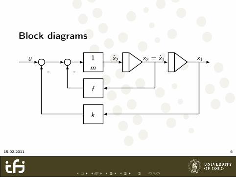
Block diagrams
1m--
f
k
x2 x2 = x1 x1u
15.02.2011 6

SISO and MIMO
Single-Input Single-Output (SISO)The system has one input u and one output xMultiple-Input Multiple-Output (MIMO)The system has multiple input u and multipleoutput xSingle-Input Multiple-Output (SIMO)Can be regarded as several SISO systemsMultiple-Input Single-Output (MISO)Can be regarded as several SISO systems
Process
Process
15.02.2011 7

Open loop vs. closed loop
Open-loop
ProcessController xur
Closed-loop
ProcessController xue
Mesurements
-
r
y
15.02.2011 8

Second order systems
H(s) =1m
s2 + fm s + k
m
=1m
(s − λ1)(s − λ2)
SolutionThe generic solution gives three cases depending on poleplacemend. The three cases are called under-damped, over-dampedand critially damped
λ{1,2} = − f2m
(1±
√1− 4
kmf 2
)(1)
15.02.2011 9
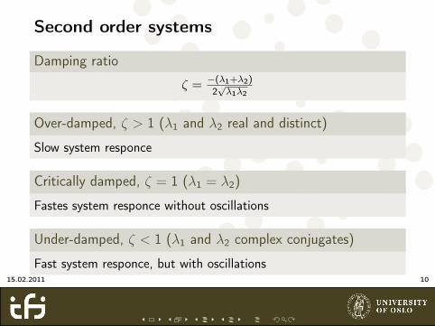
Second order systems
Damping ratio
ζ = −(λ1+λ2)
2√λ1λ2
Over-damped, ζ > 1 (λ1 and λ2 real and distinct)
Slow system responce
Critically damped, ζ = 1 (λ1 = λ2)
Fastes system responce without oscillations
Under-damped, ζ < 1 (λ1 and λ2 complex conjugates)
Fast system responce, but with oscillations15.02.2011 10
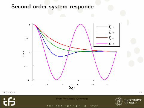
Second order system responce
From Wikimedia Commons
15.02.2011 11
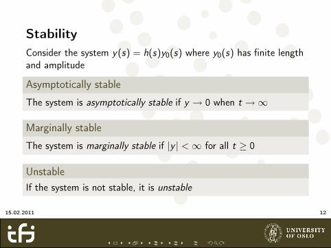
StabilityConsider the system y(s) = h(s)y0(s) where y0(s) has finite lengthand amplitude
Asymptotically stable
The system is asymptotically stable if y → 0 when t →∞
Marginally stable
The system is marginally stable if |y | <∞ for all t ≥ 0
UnstableIf the system is not stable, it is unstable
15.02.2011 12

PID controlWe want to make the system stable and controllable with acontroller. The PID controller is a simple controller that mayacheive this goal. The PID controller is often analyzed in thefrequency domain.
PID controller
u = Kpe + Ki
∫e(τ)dτ + Kd e
15.02.2011 13

Proportional
I A pure proportional controller will have a steady-state errorI Adding a integration term will remove the biasI High gain (Kp) will produce a fast systemI High gain may cause oscillations and may make the system
unstableI High gain reduces the steady-state error
15.02.2011 14
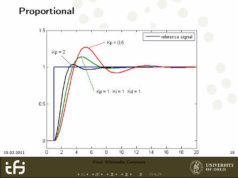
Proportional
From Wikimedia Commons
15.02.2011 15

Integral
I Removes steady-state errorI Increasing Ki accelerates the controllerI High Ki may give oscillationsI Increasing Ki will increase the settling time
15.02.2011 16

Integral
From Wikimedia Commons
15.02.2011 17
Derivative
I Larger Kd decreases oscillationsI Improves stability for low values of Kd
I May be highly sensitive to noise if one takes the derivative of anoisy error
I High noise leads to instability
15.02.2011 18

Derivative
From Wikimedia Commons
15.02.2011 19
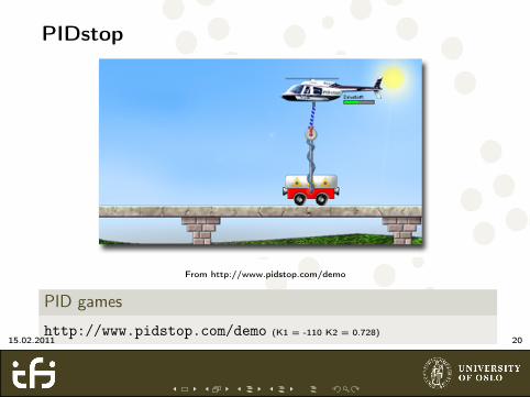
PIDstop
From http://www.pidstop.com/demo
PID games
http://www.pidstop.com/demo (K1 = -110 K2 = 0.728)15.02.2011 20
Optimal control
I Optimal controll is another control approach than PIDI The idea is to specify a cost function and then find the
optimal inputI The Dynamics of the system is used to design the controllerI For non-linear system it is not always possible to find the
optimal solutionI A special case is for linear systems with a quadradic cost
functionI The optimal controller must have all states as inputI Most often used with an observer to estimate the states that
are not measured15.02.2011 21
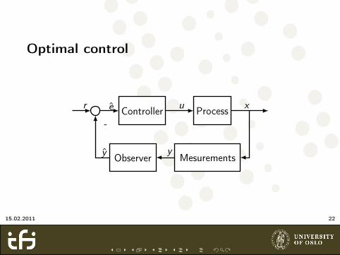
Optimal control
ProcessController xue
Mesurements
-
r
yObservery
15.02.2011 22

Linear-quadratic regulator (LQR)
I The feedback is given as u = G 1x + G 2rI r is the reference functionI The matrix G 1 and G 2 is found based on the system dynamics
and the cost function using Pontryagin’s Maximum principleI When following a trajectory the function r(t) must be known
for all future timesteps in order to find the optimal solution
Cost function
J = 12
∫ ∞t
eTQe + uTPudt
15.02.2011 23

References
J. B. Balchen, T. Andresen, and B. A. Foss.Reguleringsteknikk.Institutt for teknisk kybernetikk, 2004.
PID controller.http://en.wikipedia.org/wiki/pid_controller, February 2011.
Damping.http://en.wikipedia.org/wiki/damping, February 2011.
O.A. Solheim and Norges tekniske høgskole Institutt for tekniskkybernetikk.Optimalregulering.Tapir, 1976.
15.02.2011 24