MARINE ECOLOGY PROGRESS SERIESMar Ecol Prog Ser

Vol. 581: 71–83, 2017https://doi.org/10.3354/meps12303

Published October 13

INTRODUCTION

Foraminifera are protists that may have shellsand therefore have a long fossil record. Most eco-logical studies have been carried out to aid theinterpretation of fossil assemblages, but benthicforamin ifera play an important role in both modernand ancient ecosystems (Gooday 2003). Modernbenthic foraminifera are generalists (Van derZwaan et al. 1999), although different species havedifferent environmental requirements, and areabundant in modern environments ranging fromsupra tidal marshes to hadal trenches (see Murray2006 for a summary of distributions and ecology).

They are crucial for marine ecosystem functioning(Gooday et al. 1992). They play a role in dentitrif-cation under anoxic conditions and this functionenables benthic foraminifera to continue to calcifytheir tests (Nardelli et al. 2014). Some species re -spond rapidly to the input of phytodetritus in bothshallow-water and deep-sea systems and ap pear tobe important for processing organic matter andtransfer of energy to higher trophic levels (Gooday1988, 2003). Benthic foraminifera are important inbenthic carbon remineralisation and cycling ofother nutrients (Gooday et al. 1992). They are alsoimportant in monitoring pollution in modern seasand marginal marine environments (Alve et al.

© The authors 2017. Open Access under Creative Commons byAttribution Licence. Use, distribution and reproduction are un -restricted. Authors and original publication must be credited.

Publisher: Inter-Research · www.int-res.com

*Corresponding author: dj1@noc.ac.uk

Controls on the standing crop of benthic foraminifera at an oceanic scale

Daniel O. B. Jones1,*, John W. Murray2

1National Oceanography Centre, University of Southampton Waterfront Campus, European Way, Southampton SO14 3ZH, UK2Ocean and Earth Science, National Oceanography Centre, University of Southampton, European Way,

Southampton SO14 3ZH, UK

ABSTRACT: At present, there is very little basin-scale information on patterns of standing cropin marine organisms or their structuring forces. Understanding modern patterns and controlson foraminifera is particularly critical because of their abundance and importance in benthicsystems, as well as their role as palaeoceanographic proxies. Here, we examine for the firsttime basin-scale patterns and predictors of benthic foraminiferal standing crop from the shelfto abyssal deep sea in the Atlantic Ocean and adjacent seas using a large database of 967quantitative samples. Spatial regression analyses reveal that the flux of particulate organicmatter is a major control on standing crop size across all depths investigated, with increasingfood supply increasing fora mi ni feral standing crops. Other factors also play a role. Dissolvedoxygen is significant at slope depths and negatively related to standing crop. Temperature andpossibly salinity are locally significant factors in the abyss. This study demonstrates that pro-ductivity is important in describing foraminiferal standing crop at the basin scale, supportingits use as a palaeoceanographic proxy, but also demonstrates that other environmentalvariables are also likely important in controlling the standing crop and should be considered inreconstruction of Earth’s past marine environment.

KEY WORDS: Atlantic Ocean and adjacent seas · Meiofauna · Infauna · Density · Benthic−pelagic coupling · Palaeoceanography

OPENPEN ACCESSCCESS

Mar Ecol Prog Ser 581: 71–83, 2017

2016) and down-core studies can be used toreconstruct ecological conditions prior to the onsetof pollution to aid remediation (Alve et al. 2009).Furthermore, foraminifera are widely used inpalaeoceanographic reconstructions, especiallyusing material from deep-sea drilling (Gooday &Jorissen 2012), and for reconstructing past envi-ronments in petroleum exploration (e.g. Jones2009). Thoughtful and comprehensive reviews ofpalaeoceanographic proxies based on benthicforaminifera, discussing the history of interpreta-tions of the controls on deep sea species — fromwater depth, to water masses, to localised low-oxygen, to organic flux — have been provided byGooday (2003) and Jorissen et al. (2007 and refer-ences therein). The stable isotopic and trace ele-ment records of calcareous tests are invaluable forpalaeoceanographic reconstructions (e.g. Katz etal. 2010). At present, oxygen and organic flux arethe most recognised primary controls of fora mi -niferal distributions of species assemblages andstanding crop.

Global climate change, ocean acidification andanthropogenic activities have the potential to alterthe ecology and biogeography of populations inhab-iting the world’s seabeds, with the Atlantic being akey region of change (Jones et al. 2014). Empiricalevidence from time-series studies and manipulativeexperiments indicates that such changes will have asignificant impact on marine ecosystems and associ-ated eco system functions (Smith et al. 2008). Byunderstanding the relationships between key eco-logical variables, such as standing crop, and theirbiotic and abiotic drivers, we can begin to predict theresponses of ecosystems to future change. Theserelationships are poorly described in marine ecosys-tems owing to the limited availability of robust datafor many marine taxa, particularly in deeper waters(but see Tittensor et al. 2010). High-quality data forkey taxa at a regional scale will greatly improve ourunderstanding of macroecological patterns, both forthe taxon in question and for the purpose of provid-ing information for wider ecosystem assessments(e.g. Rex et al. 2006).

Ecological studies of benthic foraminifera carriedout on a local scale normally reveal correlationsbetween species abundance and some of the envi-ronmental variables. However, when assessed on abroader regional scale, these local correlations arenot always confirmed. The aim of this study was toconsider these ecological relationships for the deepsea and continental shelves at the scale of an oceanand to determine the main drivers.

METHODS

Treatment of standing crop and environmental data

This study is based on standing crop (density) data(Rose Bengal stained material) for the top 0−1 cm ofsediment (sample volume 10 cm3). The stainingmethod for distinguishing individuals considered tobe alive at the time of collection was introduced in1952 by Walton (Walton 1952) and has been widelyused ever since. Data on the deep sea and continentalshelves were obtained from as many literature studiesas possible from the period 1952−2013 (Murray 2015).Therefore, the dataset is not an instantaneous snap-shot but a synopsis of data gathered over 6 decades.This study focuses on the Atlantic Ocean and adjacentparts of the Arctic and Southern oceans, as well as theMediterranean and Gulf of Mexico/Caribbean. Forthis analysis, data from the deep sea and continentalshelves for all size fractions (>63µm: 554 samples;>106µm: 14 samples; >125µm: 351 samples; >150µm:49 samples) were combined (Tables S1 & S2 in Sup-plement 2 at www. int-res. com/ articles/ suppl/ m581p071 _ supp2. xlsx). There were generally larger stand-ing crops of foraminifera in the smaller size fractionsamples (see Text S1 in Supplement 1 at www. int-res.com/ articles/ suppl/ m581 p071 _ supp1. pdf). The sizefraction was incorporated into the statistical models asa covariate. In cases where the size fraction was notsignificant, it was removed in backward stepwiseelimination (see ‘Statistical analyses and modelling ofdata’). The significance value for removal was sethigh (p = 0.15), as trends were expected to reduce thelikelihood of type I error. The potential influence ofsieve-size-based differences is explored further inText S1 in Supplement 1.

Potential drivers of standing crop patterns werechosen based on established hypotheses relating totemperature (seabed temperature), productivity (fluxof particulate organic carbon [POC]), oxygen stress(dissolved oxygen [DO]), nutrient availability andsalinity, which are known to affect standing crop inthe marine environment (Tittensor et al. 2010), in -cluding that of foraminifera (Jorissen et al. 2007).Environmental variables were obtained from Inter-net-based resources as follows: temperature (Locar -nini et al. 2013), salinity (Zweng et al. 2013), oxygen(Garcia et al. 2014a) and nutrient data (Garcia et al.2014b) were obtained from World Ocean Atlas (usingthe deepest available depth band for each cell).Nutrient data, including phosphate, nitrate and sili-cate, were included to identify potential unexplainedbiochemical (e.g. marine production, respiration and

72

Jones & Murray: Standing crop of benthic foraminifera

oxidation of labile organic matter) and physical (e.g.water mass renewal and mixing) processes (Garcia etal. 2014b) not captured by the other datasets. Annualaverage POC flux data were obtained. POC flux wasestimated as a function of satellite-derived net pri-mary production and seasonal variation by Lutz et al.(2007). Data on the saturation state for calcite(ΔCO3

2− equivalent) available in global maps (Archer1996a,b) allowed examination of the distribution offoraminifera relative to the lysocline. The lysocline isat 0 on this index, negative values indicate that therecord is below the lysocline, positive is above. Datafor all variables (temperature, salinity, oxygen, nutri-ents and POC flux) were extracted for each fora -miniferal record and used as potential explanatoryvariables. Unfortunately, there are no detailed datacompilations of sediment lithology or sea-floor cur-rents at the scale necessary for this analysis, althoughboth are known to influence foraminiferal assem-blages not only on the shelf but also in the deep sea(e.g. Schönfeld 2002). Depth was not included in themodels as an environmental factor as hydrostaticpressure would not be expected to exert as strong aninfluence as other highly correlated environmentalcontrols, such as POC flux (e.g. Lutz et al. 2007; in ourdata: Spearman rank correlation between depth andPOC flux: ρ = −0.76, p < 0.001).

Statistical analyses and modelling of data

Spatial autocorrelation occurs when the values ofvariables sampled at nearby locations are not inde-pendent from each other (Dormann et al. 2007).When modelling the relationship between environ-mental predictors and response variables, spatialautocorrelation violates the assumptions of tradi-tional statistical approaches (Tittensor et al. 2010).Spatial autocorrelation was determined from a vari-ogram, which depicts the variance between pairs ofpoints at increasing distances between points (Dor-mann et al. 2007). The variance between points forour data, as is typically the case, increases up to acertain distance and then levels off (the sill). Modelfits, using the R function ‘gstat’, indicate that the sillstarts at a range of 980 km, suggesting spatial corre-lation exists up to a regional scale. This spatial auto-correlation results in deflated estimates of varianceand corresponding impacts on inference, amongother issues. As a result, variables were modelledand inferences drawn using both generalized linearmodels (GLMs) and multivariate spatial linear mod-els (SLMs). One model was initially developed for all

foraminiferal data with all environmental variablesavailable as potential explanatory variables. The sizefraction was included as a covariate as there weresignificant differences in foraminiferal standing cropwith the different sized sieves used in the analyses(see Text S1 in Supplement 1). As foraminiferal com-position is known to vary considerably between theshelf, slope and deeper waters, separate models weredeveloped for shelf (0−200 m depth), slope (200−2000 m) and abyssal (2000−6000 m) observations todetermine any additional patterns. Following pre -liminary data exploration, a log10 transformation ofthe response variables was selected to homogenisevariances and normalise data. GLMs resulted inmodel residuals that were spatially non-independent,and therefore, SLMs were used for final inference.

Spatial analysis was performed using error-spatialautoregressive models (Dormann et al. 2007), whichuse maximum-likelihood spatial autoregression.Neighbourhood thresholds between 10 and 10 000 kmwere tested at 10 km intervals and the optimal neigh-bourhood size for each model was selected by mini -mising the Akaike’s information criterion (AIC) forthe spatial null model (the model only retaining aspatial autocorrelation term). Backward stepwiseelimination of insignificant variables was then usedto determine the minimum adequate model. Thisapproach was effective in the separate analysis ofshelf, slope and abyssal data. However, in the case ofthe full dataset (all depths), no significant solutionwas found by backward stepwise elimination. For-ward selection was used, which revealed similarlysignificant models for several single-variable and 2-variable models. The importance of individual pre-dictors was assessed through t-tests (GLM) and z-tests (SLM). The models were tested further byseparately including quadratic terms and interac-tions between terms. These additional terms did notsignificantly decrease the deviance of the modelscompared with the simple models so were not ex -plored further. The significance of environmentalvariables in describing foraminiferal standing cropwas determined by examining the p-values from thestatistical models. The regression coefficients wereused to determine the magnitude and the direction ofthe relationships. Partial residual plots were used toshow the relationship between a given independentvariable and the response variable, while taking intoaccount the influence of other independent variablesalso in the model. Statistical analysis was carried outusing the R programming environment and spatialmodel analyses were carried out using R package‘spdep’ (Bivand et al. 2008).

73

Mar Ecol Prog Ser 581: 71–83, 2017

RESULTS

Patterns of standing crop of benthic foraminifera

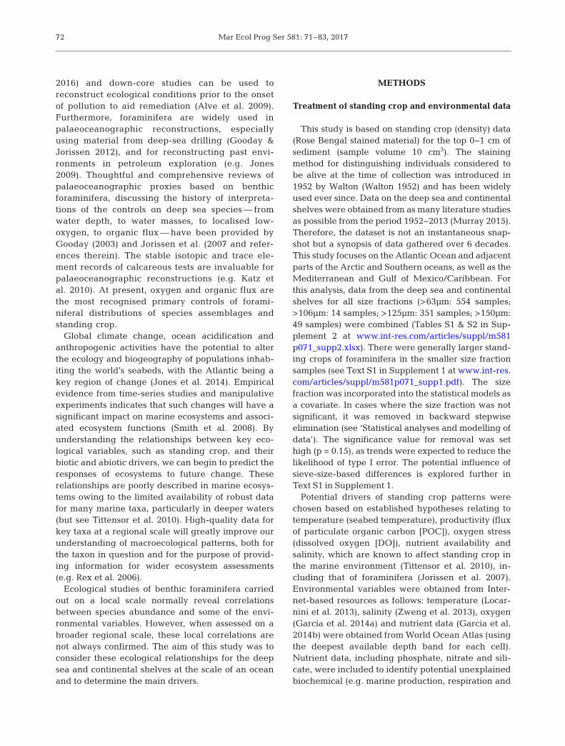
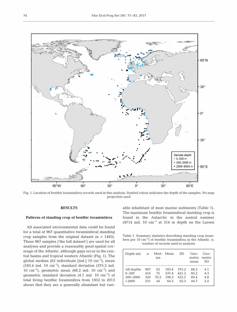
All associated environmental data could be foundfor a total of 967 quantitative foraminiferal standingcrop samples from the original dataset (n = 1483).These 967 samples (‘the full dataset’) are used for allanalyses and provide a reasonably good spatial cov-erage of the Atlantic, although gaps occur in the cen-tral basins and tropical western Atlantic (Fig. 1). Theglobal median (62 individuals [ind.] 10 cm−3), mean(183.4 ind. 10 cm−3), standard deviation (375.2 ind.10 cm−3), geometric mean (68.2 ind. 10 cm−3) andgeometric standard deviation (4.1 ind. 10 cm−3) oftotal living benthic foraminifera from 1952 to 2013shows that they are a generally abundant but vari-

able inhabitant of most marine sediments (Table 1).The maximum benthic foraminiferal standing crop isfound in the Antarctic in the austral summer(4714 ind. 10 cm−3 at 314 m depth on the Larsen

74

Depth (m) n Med- Mean SD Geo- Geo- ian metric metric

mean SD

All depths 967 62 183.4 375.2 68.2 4.10−200 416 75 237.4 421.2 85.2 4.3200−2000 320 70.2 199.3 422.2 69.4 4.8>2000 231 44 64.2 62.3 44.7 2.4

Table 1. Summary statistics describing standing crop (num-bers per 10 cm−3) of benthic foraminifera in the Atlantic. n:

number of records used in analysis

Fig. 1. Location of benthic foraminifera records used in this analysis. Symbol colour indicates the depth of the samples. No map projection used

Jones & Murray: Standing crop of benthic foraminifera

Shelf) and standing crops above4000 ind. 10 cm−3 are found in theRockall Trough (Feni Drift; 1980 mdepth) and the Grand Banks (70 mdepth), both in summer. Low ben-thic fora miniferal standing crops of<1 ind. 10 cm−3 occur in a range oflocations in cluding the North Sea,Norwegian Sea, off Iceland and inthe Gulf of Mexico at a range ofdepths (21−2800 m).

Our analysis confirms that benthicforaminifera are present across pro-duction gradients from eutrophiccoastal areas to oligotrophic areas ofthe oceans, across temperature gra-dients from polar to tropical regionsand from fully oxic to suboxic con -ditions (Table 2). Foraminifera oc -cur substantially deeper than the lysocline (lowest −23.4 µmol kg−1

ΔCO32−). They are an abundant com -

ponent of the benthos at shelf, slopeand abyssal depths (Table 1).

Environmental drivers of standingcrop of benthic foraminifera

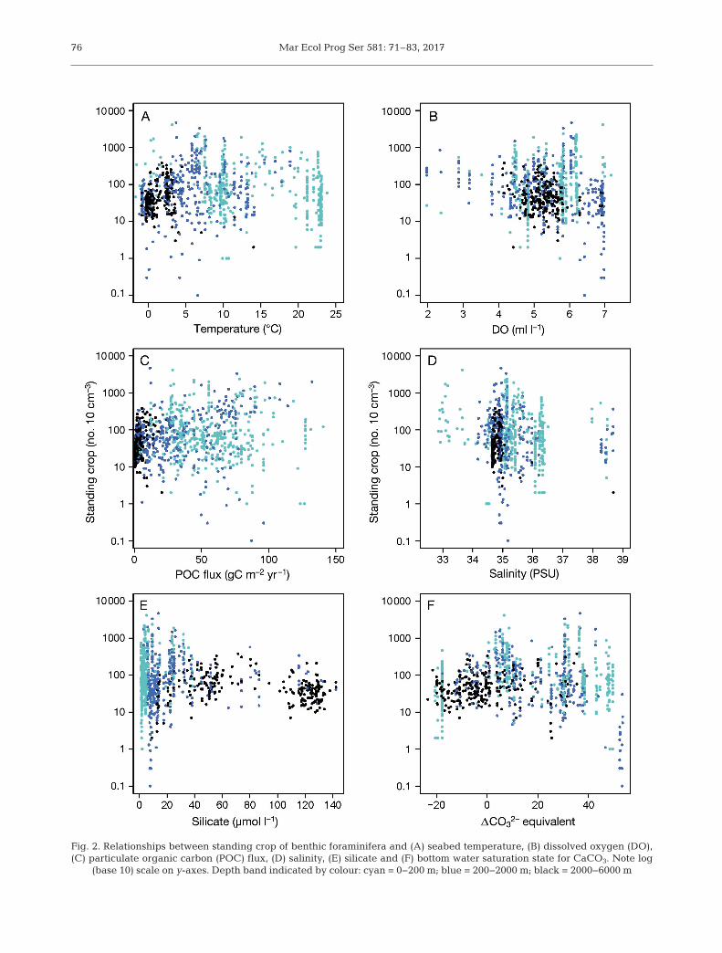
In the full dataset, significant rela-tionships exist between foramini feral standing cropand a number of single variables, including tempera-ture, DO, food supply and some nutrients (silicate andnitrate) once spatial autocorrelation is accounted for(Fig. 2, Table S3 in Supplement 1). The model can beimproved by including 2 variables; the best modelsinclude either food supply and DO or temperatureand DO (Table 3). The relatively strong positive cor-relation between food supply and temperature in thefull dataset (Spearman rank correlation ρ = 0.64, p <0.001; Fig. S1 in Supplement 1) means that there is little difference in the performance of models usingthese variables. It also means that if both temperatureand POC flux are included as variables in a modelonly one is significant. When split into depth zonesand once spatial autocorrelation has been accountedfor, significant relationships with standing crop ofbenthic foraminifera exist with different environmen-tal variables within each depth zone (Table 4).

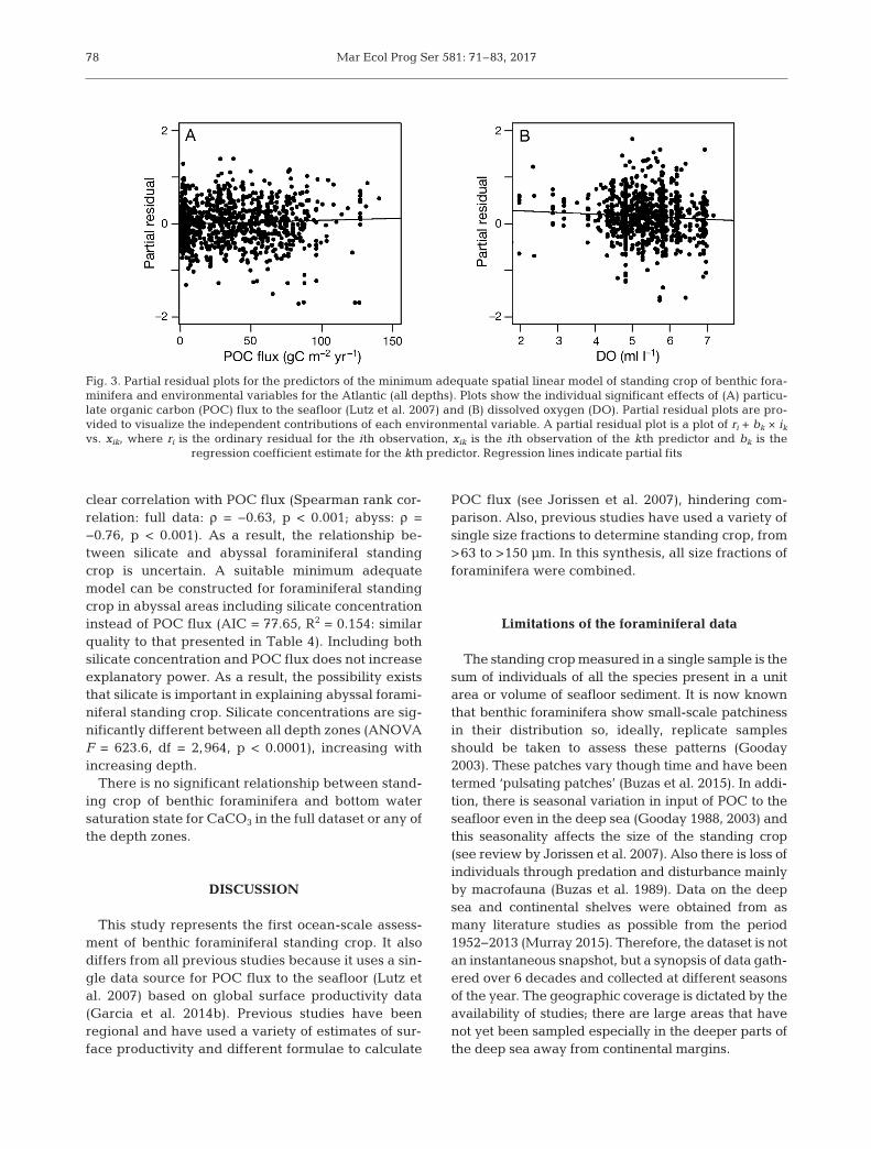
Food supply is a significant explanatory variablefor the standing crop of benthic foraminifera in thefull dataset and at all depths (Tables 3 & 4). The fulldataset shows an increase in foraminiferal standing

crop with increasing food supply (Fig. 3). On theshelf, benthic foraminiferal standing crop slightlydecreases with increasing food supply, a trend that isreversed in the deeper waters of the continentalslope and abyss (Fig. 4A,C,E).

Benthic foraminifera occur in a broad range ofseabed DO concentrations from 0.7 to 7.7 ml O2 l−1

and a significant negative linear trend is observed inthe full dataset. When divided into depth zones, asignificant trend is only observed in the slope fora -minifera (Figs. 2 & 4). The partial residual plots showthat these relationships, once the other environmen-tal variables have been held constant, are negativefor DO (Figs. 3 & 4D).

Benthic foraminifera are present across the fullspectrum of Atlantic seabed temperatures between−1.7 and 23.8°C. Temperature explains a similaramount of the variation in foraminiferal standingcrop to food supply in the full dataset and has a sig-nificant negative linear relationship (Table 3). How-ever, temperature is not significant in explaining thestanding crop of foraminifera in waters shallowerthan 2000 m, when separate analyses are carried out

75

Variable Mean SD Mini- Maxi- Me- Skew-mum mum dian ness

POC flux (gC m−2 yr−1) All 37.3 31.3 0.4 140.5 32.1 0.6Shelf 57.3 26.0 1.8 140.5 55.4 0.6Slope 35.3 27.4 0.5 132.2 26.4 0.8Abyss 4.0 4.8 0.4 34.2 2.4 3.0

Temperature (°C) All 8.3 7.5 −1.7 23.8 6.9 0.7Shelf 14.1 6.9 −1.7 23.8 10.9 0.0Slope 5.7 4.6 −1.2 18.9 5.6 0.4Abyss 1.5 1.8 −1.0 14.0 1.2 2.4

Salinity (PSU) All 35.2 0.8 32.9 38.7 35.0 1.6Shelf 35.5 0.9 32.9 38.5 35.3 0.2Slope 35.2 0.9 34.2 38.7 34.9 2.8Abyss 34.8 0.3 34.6 38.7 34.7 10.0

DO (ml l−1) All 5.3 1.0 0.7 7.2 5.3 −1.2Shelf 5.3 0.9 0.7 7.2 5.3 −1.3Slope 5.3 1.3 0.7 7.0 5.3 −1.0Abyss 5.2 0.6 1.4 6.9 5.3 −1.7

Silicate (µmol l−1) All 30.4 39.8 1.3 142.2 11.2 1.6Shelf 6.4 8.4 1.3 38.2 3.5 2.3Slope 24.4 26.6 3.1 142.2 13.6 2.6Abyss 81.9 42.3 9.0 142.2 83.6 −0.2

ΔCO32− equivalent All 11.6 21.2 −23.4 53.4 7.9 0.2

Shelf 13.9 24.8 −20.4 49.6 8.8 −0.1Slope 17.6 16.6 −17.6 53.4 17.9 0.0Abyss −0.4 13.3 −23.4 35.4 –3.2 0.8

Table 2. Summary statistics describing environmental data associated with re -cords of standing crop of benthic foraminifera used in this analysis. Shown forall depths and split by depth band: shelf (<200 m depth), slope (200−2000 m

depth) and abyss (2000–6000 m depth)

Mar Ecol Prog Ser 581: 71–83, 201776

Fig. 2. Relationships between standing crop of benthic foraminifera and (A) seabed temperature, (B) dissolved oxygen (DO),(C) particulate organic carbon (POC) flux, (D) salinity, (E) silicate and (F) bottom water saturation state for CaCO3. Note log

(base 10) scale on y-axes. Depth band indicated by colour: cyan = 0−200 m; blue = 200−2000 m; black = 2000−6000 m

Jones & Murray: Standing crop of benthic foraminifera

in each depth band. In the abyssal samples, standingcrops are higher in areas with higher sea bed temper-atures. The 3 abyssal records with temperatures>5°C occur in the Mediterranean (n = 1) and Medi-terranean outflow water (n = 2) (Fig. 4F). These 3abyssal records are also the only observations withsalinities above 35.5 PSU.

This analysis focuses on foraminifera in fully salinemarine waters (salinity range 32.9 to 38.7 PSU). In thefull dataset, there are no significant relationshipsfound between foraminiferal standing crop and salin-ity. When divided into depth zones, in the shallowersites <2000 m there is no relationship between salin-

ity and standing crop. There is a significant relation-ship with salinity and standing crop in waters>2000 m, where standing stocks are lower in areas ofincreased salinity (Fig. 4G). The high salinity data atall depths are all in the Mediterranean Sea andMediterranean outflow water.

Benthic foraminifera are found at seabed silicateconcentrations of 1.3 to 142.2 µmol l−1. There is a sig-nificant positive relationship between foramini feralstanding crop and silicate as a single variable in thefull dataset and in shelf samples (Fig. 4B), but not onthose samples taken from the slope. Silicate concen-tration in the full dataset and in the abyss displays a

77

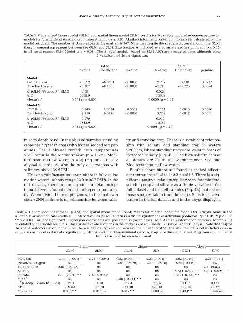
GLM SLMt-value Coefficient p-value z-value Coefficient p-value

Model 1Temperature −5.092 −0.0161 <0.0001 2.277 0.0104 0.0227Dissolved oxygen −5.307 −0.1063 <0.0001 −2.783 −0.0726 0.0054

R2 (GLM)/Pseudo R2 (SLM) 0.09 0.023AIC 1699.9 1184.8Moran’s I 0.501 (p < 0.001) −0.0009 (p = 0.49)

Model 2POC flux 3.543 0.0024 0.0004 2.101 0.0016 0.0356Dissolved oxygen −3.919 −0.0736 <0.0001 −3.258 −0.0817 0.0011

R2 (GLM)/Pseudo R2 (SLM) 0.079 0.016AIC 1713.0 1185.5Moran’s I 0.532 (p < 0.001) 0.0008 (p = 0.45)

Table 3. Generalized linear model (GLM) and spatial linear model (SLM) results for 2-variable minimal adequate regressionmodels for foraminiferal standing crop using Atlantic data. AIC: Akaike’s information criterion. Moran’s I is calculated on themodel residuals. The number of observations in the analysis is 967. Note that despite the spatial autocorrelation in the GLM,there is general agreement between the GLM and SLM. Size fraction is included as a covariate and is significant (p < 0.05)in all cases (except SLM Model 1: p = 0.06). The 2 ‘best’ models (based on SLM AIC) are presented here, although other

2-variable models are significant

Shelf Slope AbyssGLM SLM GLM SLM GLM SLM

POC flux −3.19 (−0.004)** −2.21 (−0.003)* 6.53 (0.009)*** 3.25 (0.004)** 2.62 (0.016)** 2.21 (0.011)*Dissolved oxygen ns ns −2.86 (−0.089)** −2.45 (−0.078)* −2.76 (−0.110)** nsTemperature −5.65 (−0.023)*** ns ns ns ns 2.21 (0.027)***Salinity ns ns ns ns −5.75 (−0.512)*** −5.91 (−0.698)***Silicate 8.41 (0.029)*** 2.13 (0.015)* ns ns −3.54 (−0.003)*** nsΔCO3

2− ns ns −5.38 (−0.014)*** ns ns nsR2 (GLM)/Pseudo R2 (SLM) 0.219 0.010 0.253 0.035 0.181 0.141AIC 709.32 557.78 541.00 428.33 162.03 79.47Moran’s I 0.383*** −0.011 ns 0.417*** 0.003 ns 0.433*** −0.056 ns

Table 4. Generalized linear model (GLM) and spatial linear model (SLM) results for minimal adequate models for 3 depth bands in the Atlantic. Numbers indicate t-values (GLM) or z-values (SLM). Asterisks indicate significance of individual predictors: *p < 0.05; **p < 0.01;***p < 0.001. ns: not significant. Regression coefficients are presented in parentheses. AIC: Akaike’s information criterion. Moran’s I is calculated on the model residuals. The numbers of observations in the analysis are 416 (shelf), 320 (slope) and 231 (abyss). Note that despitethe spatial autocorrelation in the GLM, there is general agreement between the GLM and SLM. The size fraction is not included as a co -variate in any model as it is not a significant (p > 0.15) predictor of foraminiferal standing crop once the variation resulting from environmental

factors has been taken into account

Mar Ecol Prog Ser 581: 71–83, 2017

clear correlation with POC flux (Spearman rank cor-relation: full data: ρ = −0.63, p < 0.001; abyss: ρ =−0.76, p < 0.001). As a result, the relationship be -tween silicate and abyssal foraminiferal standingcrop is uncertain. A suitable minimum adequatemodel can be constructed for foraminiferal standingcrop in abyssal areas including silicate concentrationinstead of POC flux (AIC = 77.65, R2 = 0.154: similarquality to that presented in Table 4). Including bothsilicate concentration and POC flux does not increaseexplanatory power. As a result, the possibility existsthat silicate is important in explaining abyssal for a mi - niferal standing crop. Silicate con centrations are sig-nificantly different between all depth zones (ANOVAF = 623.6, df = 2,964, p < 0.0001), increasing withincreasing depth.

There is no significant relationship between stand-ing crop of benthic foraminifera and bottom watersaturation state for CaCO3 in the full dataset or any ofthe depth zones.

DISCUSSION

This study represents the first ocean-scale assess-ment of benthic foraminiferal standing crop. It alsodiffers from all previous studies because it uses a sin-gle data source for POC flux to the seafloor (Lutz etal. 2007) based on global surface productivity data(Garcia et al. 2014b). Previous studies have beenregional and have used a variety of estimates of sur-face productivity and different formulae to calculate

POC flux (see Jorissen et al. 2007), hindering com-parison. Also, previous studies have used a variety ofsingle size fractions to determine standing crop, from>63 to >150 µm. In this synthesis, all size fractions offoraminifera were combined.

Limitations of the foraminiferal data

The standing crop measured in a single sample is thesum of individuals of all the species present in a unitarea or volume of seafloor sediment. It is now knownthat benthic foraminifera show small-scale patchinessin their distribution so, ideally, replicate samplesshould be taken to assess these patterns (Gooday2003). These patches vary though time and have beentermed ‘pulsating patches’ (Buzas et al. 2015). In addi-tion, there is seasonal variation in input of POC to theseafloor even in the deep sea (Gooday 1988, 2003) andthis seasonality affects the size of the standing crop(see review by Jorissen et al. 2007). Also there is loss ofindividuals through predation and disturbance mainlyby macrofauna (Buzas et al. 1989). Data on the deepsea and continental shelves were obtained from asmany literature studies as possible from the period1952−2013 (Murray 2015). Therefore, the dataset is notan instantaneous snapshot, but a synopsis of data gath-ered over 6 decades and collected at different seasonsof the year. The geographic coverage is dictated by theavailability of studies; there are large areas that havenot yet been sampled especially in the deeper parts ofthe deep sea away from continental margins.

78

Fig. 3. Partial residual plots for the predictors of the minimum adequate spatial linear model of standing crop of benthic fora -minifera and environmental variables for the Atlantic (all depths). Plots show the individual significant effects of (A) particu-late organic carbon (POC) flux to the seafloor (Lutz et al. 2007) and (B) dissolved oxygen (DO). Partial residual plots are pro-vided to visualize the independent contributions of each environmental variable. A partial residual plot is a plot of ri + bk × ikvs. xik, where ri is the ordinary residual for the ith observation, xik is the ith observation of the kth predictor and bk is the

regression coefficient estimate for the kth predictor. Regression lines indicate partial fits

Jones & Murray: Standing crop of benthic foraminifera

The Rose Bengal staining method for distinguish-ing individuals considered to be alive at the time ofcollection was introduced in 1952 and has beenwidely used ever since. However, Rose Bengal is nota vital stain and therefore some workers have sug-gested that recently dead individuals may alsobecome stained and thus give an overestimate of thenumbers alive (see Murray & Bowser 2000 and Bern-hard et al. 2006 for discussion).

Notwithstanding these limitations, we believe thatthe dataset used in this ocean-wide study is adequateto determine the major controlling factors governingthe size of the standing crop.

Limitations of the approach

Data collected using multiple methods were com-bined in this study to provide a broad-scale overviewof potential environmental drivers of foraminiferalstanding crop. This approach is at present the onlyway to address important regional questions, butcomes with a number of limitations (further discus-sion in Text S1 in Supplement 1). First, the combina-tion of data collected with different size fractionsintroduces a covariate, which will increase error inestimates. Foraminiferal standing crop was, as wouldbe expected (McClain et al. 2012), significantly

79

Fig. 4. Partial residual plots for thepredictors of the minimum ade-quate spatial linear model standingcrop of benthic foraminifera and en-vironmental variables for 3 depthbands in the Atlantic: (A,B) 0−200 m(cyan); (C,D) 200−2000 m (blue);(E−G) >2000 m (black). Plots showthe individual significant effects of(A,C,E) particulate organic carbon(POC) flux to the seafloor (Lutz etal. 2007), (B) silicate, (D) dissolvedoxygen (DO), (F) temperature and(G) salinity. Partial residual plotsare provided to visualize the inde-pendent contributions of each envi-ronmental variable. See Fig. 3 fordescription of a partial re sidual plot.Regression lines indicate partial fits

Mar Ecol Prog Ser 581: 71–83, 2017

higher in samples taken with smaller sieves andthere were some spatial patterns in the size fractionanalysed (Fig. S2 in Supplement 1). Second, therewas inevitable correlation between environmentalvariables (Fig. S1 in Supplement 1), which limits ourability to determine which of a correlated set of environmental variables the key driver is. It shouldalso be stressed that although data were collectedthrough out the year and over 6 decades (Murray2015), there were insufficient samples to resolve sea-sonal or interannual variability.

Role of POC in determining foraminiferal standing crop

Food supply appears the most likely of the corre-lated environmental variables, such as temperatureand silicate, to be the primary driver for foraminiferalstanding crops. This assumption is supported by ouranalyses, for example, by the consistent relationshipsbetween food supply and standing crop in the fulldata and across the separate depth zones, and a largebody of literature (Murray 2015). Our results show ageneral pattern of increasing foraminiferal standingcrop with increased food supply, but more detailedassessment shows that there is a different response toPOC between shelf and deeper areas in the Atlantic.In general, on the slope and in the abyss, the positiverelationship between standing crop and POC gener-ally reported in localised studies of the deep sea (e.g.Schmiedl et al. 1997) is also found here at the scale ofan ocean (Fig. 4C,E). Increases in standing crop withfood supply are expected and supported by eco -logical theory (e.g. McClain et al. 2012). Surprisingly,on the shelf there is a significant negative relation-ship between POC flux and standing crop (Fig. 4A).This relationship deserves further experimental as -sessment. However, the explanation for this negativerelationship could be a function of some other co- correlating factor. For example, increases in POCflux may lead to increases in predation pressure,causing localised losses in standing crop (Buzas et al.1989). Areas with high POC flux on the shelf couldalso be associated with other environmental controls.Studies of shelf sea foraminiferal distributions showsediment lithology and tidal and/or wave energy tobe important controls on species abundance. Areasof high energy with sandy substrates have muchlower standing crops than low energy muddy sub-strates (Murray 2006, p. 158). In shallow areas, thesatellite-derived estimates of POC flux to the seafloorare likely less accurate — lateral advection, resus-

pension and preferential accumulation in areas offine-grained sediment may all influence spatial pat-terns. Perhaps the most likely explanation for un -expected patterns is that resource quality cannot bedetermined from the satellite-derived measure ofPOC flux used in this analysis. Refractory material,which is more common on the shelf, is a poor foodresource compared with labile organic matter (Licariet al. 2003, Fontanier et al. 2008). In general, there isa large spread of standing crop for a given value ofPOC flux at all depths, which could also be explainedby variation resulting from these factors.

Abiotic factors

There is a negative correlation between DO andstanding crop in the full dataset and on the slope. It isknown that when oxygen availability is restricted itadversely affects the benthic foraminifera. However,above a threshold of ~1.0 ml O2 l−1 = 45 µM, oxygenis no longer a limiting factor for foraminifera (Gooday2003) so the majority of open-sea assemblages arenot limited by oxygen. An oxygen minimum zone isintermittently developed along the African slope, inthe vicinity of Angola and Namibia. DO values<1.0 ml O2 l−1 only occur at 3 stations in our data from193, 531 and 1965 m in an oxygen minimum zone offthe Cunene River at 17° S in the SE Atlantic (originaldata in Schmiedl et al. 1997). It is possible that lower-oxygen areas had lower numbers of active mega -fauna that may compete with foraminifera for labilephytodetritus. Reduced POC flux attenuation in theoxygen minimum zone, and a resultant higher sea -bed POC flux than model predictions, may occur as aconsequence of reduced mesopelagic zooplanktonfeeding and microbial degradation activities (e.g.Keil et al. 2016).

Dissolved silicate is a significant factor on the shelfand abyss, but not between 200 and 2000 m. As silicais not utilised in test construction by benthic fora -minifera, its correlation with standing crop was un -expected. One possible explanation is that it is anindication of the type of organic detritus, e.g. diatomsor silicoflagellates. As shown in ‘Results’, either sili-cate or POC could be the drivers in the abyss.

Bottom water temperature has long been known tobe a control on species distributions, especially inshelf and marginal marine environments. It is diffi-cult to separate the effects of temperature from thoseof food supply. Our data indicate that temperaturemay have a particular influence on the amount offoraminiferal standing crop in the deep sea, which

80

Jones & Murray: Standing crop of benthic foraminifera

has not previously been recognised in the foramini -feral literature. The body of ecological theory (e.g.the metabolic theory of ecology; Brown et al. 2004)and observations for other taxa would support a tem-perature relationship, relating temperature increasesto elevated metabolic rate, biomass and populationsizes (McClain et al. 2012). However, it should berecognised that the range of temperatures exhibitedin the deep sea is relatively small compared withother environments.

It is likely that the trends observed here associatedwith temperature and salinity were driven by outly-ing low foraminiferal standing crops associated withthe oligotrophic, high-temperature and high-salinityMediterranean and Mediterranean outflow water onthe Portuguese slope. Low foraminiferal standingcrops in Mediterranean outflow has been observedbefore and associated with a decrease in labile POCat the sediment surface (Fontanier et al. 2008).

The saturation state for CaCO3 may be more impor-tant as a factor influencing taphonomy (dissolution ofcalcareous tests) rather than as a control on livingforms. A wide variety of benthic calcifiers live inwaters undersaturated with CaCO3, using a range ofsophisticated mechanisms for constructing and main-taining their CaCO3 structures (Lebrato et al. 2016).

Although there were no data on bottom currentsfor each sampling site, such currents are consideredto be responsible for locally controlling standingcrops. In areas of high current speed (up to 50 cm s−1),the seabed is winnowed and standing crops are low(Schönfeld 2002). In Walvis Bay, bottom nepheloidlayers flowing from shelf down slope transport or -ganic detritus to greater depths and lead to higherstanding crops than at shallower depths (54 and189 ind. 10 cm−3 at 892 and 1957 m respectively;Fontanier et al. 2013).

In summary, at the scale of an ocean, POC flux isimportant in controlling foraminiferal standing cropacross all depths, as previously determined in regio -nal studies. Locally, on the continental slope, DOconcentration is important and in deeper waters tem-perature and salinity have a significant effect onforaminiferal standing crops.

Relevance to palaeoceanographic studies

Benthic foraminiferal tests are the main benthicmeiofauna in fossil deep-sea sediments and macro-faunal remains are relatively rare. Therefore, benthicforaminifera offer the best prospect for interpretingpast deep-sea environments (Jorissen et al. 2007).

Two approaches are taken: study of individual spe-cies and study of assemblages of tests. Only the latteris relevant to this study. The correlation betweenstanding crop and POC flux forms the basis for theestablishment of a palaeoceanographic proxy forproductivity, namely the benthic foraminiferal accu-mulation rate (BFAR). The merits and problems asso-ciated with BFAR have been reviewed in detail byGooday (2003) and Jorissen et al. (2007) and will notbe repeated here. However, there is a fundamentaldifference between BFAR, which is a rate processand includes a time element (usually of thousands ofyears), and standing crop, which is a stock at a spe-cific time. In view of the wide range of standing cropsfor a given value of POC flux observed here, togetherwith the range of other factors that influence stand-ing crop, it is likely that the BFAR should be viewedas a measure of relative rather than absolute produc-tivity change.

CONCLUSIONS

The aim of this study was to test whether relation-ships between standing crop and environmental fac-tors observed in regional studies were still observedat the scale of the Atlantic Ocean. Six decades offoraminiferal standing crop data analysed herestrongly support the correlation between standingcrop and POC flux for the ocean and indicate theimportance of DO, but more detailed analysis revealsdifferences between the continental shelf and deeperwaters >200 m. On the shelf, observed patterns offoraminiferal standing crop are complex. There is adecrease in standing crop with increase in POC fluxand there is a positive correlation with dissolved sil-ica, possibly indicating that siliceous organisms en -hance foraminiferal standing crops or that other fac-tors correlating with POC flux are important, e.g.lateral advection of POC. In deeper water (>200 m),the oceanic-scale data presented here confirm theobservations from local studies that the primary fac-tor controlling benthic foraminiferal standing crop isthe flux of POC. Bottom waters are well-oxygenatedexcept on localised areas of the African slope andnever fall to values that affect the benthic foraminif-era. Only extremes of temperature and salinity indeep water associated with the Mediterraneanappear to be associated with lower standing crop val-ues. There is no significant relationship betweenstanding crop and the saturation state for CaCO3 atany depth. Although it might be expected that thesize fraction examined would influence the magni-

81

Mar Ecol Prog Ser 581: 71–83, 2017

tude of standing crop, it appears that variation be -tween samples as a result of environmental variationis orders of magnitude larger than the variation causeby changes in size fraction (Text S1 in Supplement 1).

This paper has implications for palaeoceanogra-phy. Our results highlight the correlations betweenstanding crop and productivity, supporting the use ofbenthic foraminiferal accumulation rate (BFAR) as apalaeoceanographic proxy for productivity, at least indeeper waters. However, our results suggest widevariability in response as well as additional factorsthat influence standing crop, at least for short-termmeasurements of standing crop, which have not beenintegrated over time. The large dataset assembledhere is important more generally for deep-sea eco -logists. It can feed into other deep-sea macroecologi-cal studies, as well as provide baseline data for asses -sing the impacts of global change.

Acknowledgements. We thank the many authors who overthe years have supplied spreadsheets of foraminiferal data,without which this study would have been impossible.D.O.B.J. was supported for this work by the UK NaturalEnvironment Research Council through National Capabilityfunding to the National Oceanography Centre.

LITERATURE CITED

Alve E, Lepland A, Magnusson J, Backer-Owe K (2009)Monitoring strategies for re-establishment of ecologicalreference conditions: possibilities and limitations. MarPollut Bull 59: 297−310

Alve E, Korsun S, Schönfeld J, Dijkstra N and others (2016)Foram-AMBI: a sensitivity index based on benthic fora -miniferal faunas from the North-East Atlantic and Arcticfjords, continental shelves and slopes. Mar Micropaleon-tol 122: 1−12

Archer DE (1996a) A data-driven model of the global calcitelysocline. Global Biogeochem Cycles 10: 511−526

Archer DE (1996b) An atlas of the distribution of calciumcarbonate in sediments of the deep sea. Global Bio-geochem Cycles 10: 159−174

Bernhard JM, Ostermann D, Williams DS, Blanks JK (2006)Comparison of two methods to identify live benthicforaminifera: a test between Rose Bengal and Cell-Tracker Green with implications for stable isotope paleo-reconstructions. Paleoceanography 21: PA4210

Bivand RS, Pebesma E, Gómez-Rubio V (2008) Applied spa-tial data analysis with R. Springer, New York, NY

Brown JH, Gillooly JF, Allen AP, Savage VM, West GB(2004) Towards a metabolic theory of ecology. Ecology85: 1771−1789

Buzas MA, Collins LS, Richardson SL, Severin KP (1989)Experiments on predation, substrate preference, and col-onization of benthic foraminifera at the shelfbreak off theFt. Pierce Inlet, Florida. J Foraminiferal Res 19: 146−152

Buzas MA, Hayek LA, Jett JA, Read DA (2015) Pulsatingpatches. History and analyses of spatial, seasonal, andyearly distribution of living benthic foraminifera. Smith-

sonian Contributions to Paleobiology 97, SmithsonianInstitution Scholarly Press, Washington, DC

Dormann CF, McPherson JM, Araújo MB, Bivand RS andothers (2007) Methods to account for spatial autocorrela-tion in the analysis of species distributional data: areview. Ecography 30: 609−628

Fontanier C, Jorissen FJ, Lansard B, Mouret A and others(2008) Live foraminifera from the open slope betweenGrand Rhône and Petit Rhône canyons (Gulf of Lions,NW Mediterranean). Deep Sea Res I 55: 1532−1553

Fontanier C, Metzger E, Waelbroeck MJ, LeFloch N andothers (2013) Live (stained) benthic foraminifera offWalvis Bay, Namibia: a deep-sea ecosystem under theinfluence of bottom nepheloid layers. J Foraminiferal Res43: 55−71

Garcia HE, Locarnini RA, Boyer TP, Antonov JI and others(2014a) In: Levitus S, Mishonov A (eds) World ocean atlas2013, Vol 3. Dissolved oxygen, apparent oxygen uti -lization, and oxygen saturation. NOAA Atlas NESDIS 75,NOAA, Silver Spring, MD, p 1–27

Garcia HE, Locarnini RA, Boyer TP, Antonov JI and others(2014b) In: Levitus S, Mishonov A (eds) World oceanatlas 2013, Vol 4. Dissolved inorganic nutrients (phos-phate, nitrate, silicate). NOAA Atlas NESDIS 76, NOAA,Silver Spring, MD, p 1–25

Gooday AJ (1988) A response by benthic foraminifera to thedeposition of phytodetritus in the deep sea. Nature 332: 70−73

Gooday AJ (2003) Benthic foraminifera (Protista) as tools indeep-water palaeoceanography: environmental influ-ences on faunal characteristics. Adv Mar Biol 46: 1−90

Gooday AJ, Jorissen F (2012) Benthic foraminiferal bio -geography: controls on global distribution patterns indeep-water settings. Annu Rev Mar Sci 4: 237−262

Gooday AJ, Levin L, Linke P, Heeger T (1992) The role ofbenthic foraminifera in deep-sea food webs and carboncycles. In: Rowe GT, Pariente V (eds) Deep-sea foodchains and the global cycle. Kluwer Academic Publish-ers, Dordrecht, p 63−91

Jones RW (2009) Stratigraphy, palaeoenvironmental inter-pretation and uplift history of Barbados based on fora -miniferal and other palaeontological evidence. J Micro -palaeontol 28: 37−44

Jones DOB, Yool A, Wei CL, Henson SA, Ruhl HA, WatsonRA, Gehlen M (2014) Global reductions in seafloor bio-mass in response to climate change. Glob Change Biol20: 1861−1872

Jorissen FJ, Fontanier C, Thomas E (2007) Paleoceanographicproxies based on deep-sea benthic formanini feral assem-blage characteristics. In: Hillaire-Marcel E, de Vernal C(eds) Proxies in Late Cenozoic paleoceano graphy: Pt 2: bio logical tracers and biomarkers. Developments in Marine Geology 1, Elsevier, Amsterdam, p 263−326

Katz M, Cranmer BS, Framzese A, Hönisch B, Miller KG,Rosenthal Y, Wright JD (2010) Traditional and emerginggeochemical proxies in foraminifera. J Foraminiferal Res40: 165−192

Keil RG, Neibauer J, Biladeau C, van der Elst K, Devol AH(2016) A multiproxy approach to understanding the “en -hanced” flux of organic matter through the oxygen- deficient waters of the Arabian Sea. Biogeosciences 13: 2077−2092

Lebrato M, Andersson AJ, Ries JB, Aronson RB and others(2016) Benthic marine calcifiers coexist with CaCO3-undersaturated seawater worldwide. Global Biogeo -

82

Jones & Murray: Standing crop of benthic foraminifera

chem Cycles 30: 1038−1053Licari LN, Schumacher S, Wenzhöfer F, Zabel M, Mack-

ensen A (2003) Communities and microhabitats of livingbenthic foraminifera from the tropical east Atlantic: impact of different productivity regimes. J ForaminiferalRes 33: 10−31

Locarnini RA, Mishonov AV, Antonov JI, Boyer TP and oth-ers (2013) In: Levitus S, Mishonov A (eds) World oceanatlas 2013, Vol 1. Temperature. NOAA Atlas NESDIS 73,NOAA, Silver Spring, MD, p 1–40

Lutz MJ, Caldeira K, Dunbar RB, Behrenfeld MJ (2007) Sea-sonal rhythms of net primary production and particulateorganic carbon flux to depth describe the efficiency ofbiological pump in the global ocean. J Geophys Res 112: C10011

McClain CR, Allen AP, Tittensor DP, Rex MA (2012) Ener-getics of life on the deep seafloor. Proc Natl Acad SciUSA 109: 15366−15371

Murray JW (2006) Ecology and applications of benthicforaminifera. Cambridge University Press, Cambridge

Murray JW (2015) Some trends in sampling modern living(stained) benthic foraminifera in fjord, shelf and deepsea: Atlantic Ocean and adjacent seas. J Micropalaeontol34: 101−104

Murray JW, Bowser SS (2000) Mortality, protoplasm decayrate, and reliability of staining techniques to recognize‘living’ foraminifera: a review. J Foraminiferal Res 30: 66−70

Nardelli MP, Barras C, Metzger E, Mouret A, Filipsson HL,Jorissen F, Geslin E (2014) Experimental evidence forforaminiferal calcification under anoxia. Biogeosciences

11: 4029−4038Rex MA, Etter RJ, Morris JS, Crouse J and others (2006)

Global bathymetric patterns of standing stock andbody size in the deep-sea benthos. Mar Ecol Prog Ser317: 1−8

Schmiedl G, Mackensen A, Müller PJ (1997) Recent benthicforaminifera from the eastern South Atlantic Ocean: dependence on food supply and water masses. MarMicropaleontol 32: 249−287

Schönfeld J (2002) Recent benthic foraminiferal assem-blages in deep high-energy environments from the Gulfof Cadiz (Spain). Mar Micropaleontol 44: 141−162

Smith CR, De Leo FC, Bernardino AF, Sweetman AK, ArbizuPM (2008) Abyssal food limitation, ecosystem structureand climate change. Trends Ecol Evol 23: 518−528

Tittensor DP, Mora C, Jetz W, Lotze HK, Ricard D, VandenBerghe E, Worm B (2010) Global patterns and pre -dictors of marine biodiversity across taxa. Nature 466: 1098–1101

Van der Zwaan GJ, Duinstee IAP, Den Dulk M, Ernst S, Jan-ninck NT, Kouwenhoven TJ (1999) Benthic foraminifers: proxies or problems?: A review of paleoecological con-cepts. Earth Sci Rev 46: 213−236

Walton WR (1952) Techniques for recognition of livingforaminifera. Contrib Cushman Found Foraminifer Res 3: 56−60

Zweng MM, Reagan JR, Antonov JI, Locarnini RA and oth-ers (2013) In: Levitus S, Mishonov A (eds) World oceanatlas 2013, Vol 2. Salinity. NOAA Atlas NESDIS 74,NOAA, Silver Spring, MD, p 1–39

83

Editorial responsibility: Marsh Youngbluth, Fort Pierce, Florida, USA

Submitted: April 25, 2017; Accepted: August 10, 2017Proofs received from author(s): October 3, 2017