controlling fluid-induced seismicity during a 6.1-km-deep … · controlling fluid-induced...

SC I ENCE ADVANCES | R E S EARCH ART I C L E

EARTH SC I ENCES

1Helmholtz Centre Potsdam, GFZ German Research Centre for Geosciences, Sec-tion 4.2: Geomechanics and Scientific Drilling, Potsdam, Germany. 2Free UniversityBerlin, Berlin, Germany. 3St1 Deep Heat Oy, Helsinki, Finland. 4Arup, London, UK.5University of Potsdam, Potsdam, Germany. 6Department of Geosciences andGeography, University of Helsinki, Helsinki, Finland. 7ASIR Advanced SeismicInstrumentation and Research, Dallas, TX, USA.*Corresponding author. Email: [email protected]

Kwiatek et al., Sci. Adv. 2019;5 : eaav7224 1 May 2019

Copyright © 2019

The Authors, some

rights reserved;

exclusive licensee

American Association

for the Advancement

of Science. No claim to

originalU.S. Government

Works. Distributed

under a Creative

Commons Attribution

NonCommercial

License 4.0 (CC BY-NC).

Dow

nl

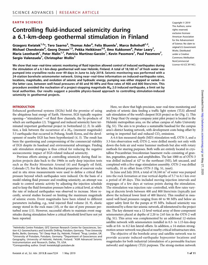
Controlling fluid-induced seismicity duringa 6.1-km-deep geothermal stimulation in FinlandGrzegorz Kwiatek1,2*, Tero Saarno3, Thomas Ader4, Felix Bluemle1, Marco Bohnhoff1,2,Michael Chendorain4, Georg Dresen1,5, Pekka Heikkinen3,6, Ilmo Kukkonen6, Peter Leary7,Maria Leonhardt1, Peter Malin1,7, Patricia Martínez-Garzón1, Kevin Passmore7, Paul Passmore7,Sergio Valenzuela7, Christopher Wollin1

We show that near–real-time seismic monitoring of fluid injection allowed control of induced earthquakes duringthe stimulation of a 6.1-km-deep geothermal well near Helsinki, Finland. A total of 18,160 m3 of fresh water waspumped into crystalline rocks over 49 days in June to July 2018. Seismic monitoring was performed with a24-station borehole seismometer network. Using near–real-time information on induced-earthquake rates,locations, magnitudes, and evolution of seismic and hydraulic energy, pumping was either stopped or varied—inthe latter case, between well-head pressures of 60 and 90 MPa and flow rates of 400 and 800 liters/min. Thisprocedure avoided the nucleation of a project-stopping magnitude MW 2.0 induced earthquake, a limit set bylocal authorities. Our results suggest a possible physics-based approach to controlling stimulation-inducedseismicity in geothermal projects.

oaded
on M
ay 27, 2020http://advances.sciencem

ag.org/ from

INTRODUCTIONEnhanced geothermal systems (EGSs) hold the promise of usingthe ubiquitous heat energy of Earth. However, EGS typically requiresopening—“stimulation”—of fluid flow channels, the by-products ofwhich are earthquakes (1). Triggered and induced seismicity have ter-minated important geothermal project in Switzerland (2, 3). In addi-tion, a link between the occurrence of a MW (moment magnitude)5.5 earthquake that occurred in Pohang, South Korea, and the devel-opment of nearby EGS has been hypothesized (4, 5). The result hasbeen the questioning and compromising of the commercial viabilityof EGS despite its baseload and environmental advantages. Findingsafe stimulation strategies is thus critical for reducing the negativesocioeconomic impact of EGS-related induced seismicity.

Previous efforts aiming at controlling seismicity during fluid in-jection projects date back to the 1960s in early deep injection testssuch as the Rocky Mountain Arsenal (6) and Rangely oil field,Colorado (7). For the latter, the frictional properties of reservoir rocksand in situ stress measurements were used to define a critical fluidpressure beyond which earthquakes were induced. On the basis of amodel relating fluid pressure and resulting seismicity, an attempt wasmade to control seismic activity by adjusting the injection scheduleand to keep the fluid formation pressure below a critical level, at whichthe rate of induced earthquakes was observed to increase. More re-cently, several studies focused on limiting the maximum magnitudeof seismic events. Event magnitudes have been related to differentparameters including, e.g., total injected fluid volume (8, 9), elasticenergy stored in the rock mass (10), or the size of pore pressure per-turbed zone (11). However, successful efforts to maintain event mag-nitudes during stimulation below a critical threshold level have not yetbeen reported.

Here, we show that high-precision, near–real-time monitoring andanalysis of seismic data feeding a traffic light system (TLS) allowedsafe stimulation of the world’s deepest EGS project so far (Fig. 1). ThisSt1 Deep Heat Oy energy-company joint pilot project is located in theHelsinki metropolitan area, on the urban campus of Aalto University(fig. S1). The aim is to produce a sustainable baseload for the campusarea’s district heating network, with development costs being offset bysaving in imported fuel and reduced CO2 emissions.

A 6.4-km measured depth (MD) stimulation well, OTN-3, and a3.3-km observation well, OTN-2, were drilled mostly not only withdown-the-hole air and water hammer methods but also with rotarymethods for steering purposes. Both wells are entirely located in crys-talline Precambrian Svecofennian basement rocks consisting of gran-ites, pegmatites, gneisses, and amphibolites. The last 1000 m of OTN-3was drilled inclined at 42° to the northeast (NE), left uncased, andcompleted with a five-stage stimulation assembly. OTN-2 was drilledvertically, 10 m offset from OTN-3 (fig. S1, inset).

In June and July 2018, a total of 18,160 m3 of water was pumpedinto the rock formation at true vertical depths of 5.7 to 6.1 km overa period of 49 days. This included moving injection intervals andstoppages of a few days at various points during the stimulation.The stimulation was injection rate–controlled, with flow rates vary-ing at discrete levels between 400 and 800 liters/min (typically justabove the technical lower limit of 400 liters/s). This resulted in mea-sured well-head pressures ranging from 60 to 90 MPa and below anupper safety limit for the pumps at 95 MPa. Induced seismicity wasmonitored by a three-tier seismic network, all telemetered to the projectsite. The key element was a 12-level vertical array of three-componentseismometers placed at depths of 2.20 to 2.65 km in the OTN-2 well(fig. S1). This array was complemented by an additional 12-stationsatellite network with seismometers installed in 0.3- to 1.15-km-deepwells at 0.6- to 8.2-km lateral offsets. In addition, a 14-station strong-motion sensor networkwas placed at nearby critical infrastructure sites.

The objective of the borehole array and satellite network was toprovide accurate induced-earthquake hypocenter locations andmagnitudes for both industrial (stimulation of a permeable fracturenetwork) and regulatory (TLS) purposes. The strong-motion network

1 of 11

http://advances.sciencemag.org/


on May 27, 2020


Dow

nloaded from

was aimed at providing direct evidence of potentially damagingshaking. Background seismicity in the campus region is very sparse.The closest event with claims of building damage in recent years wasa MW 2.4 event in 2011, located 50 km to the NE from the projectsite. Two detected microearthquakes were reported to have occurredwithin 2 km of the drill site in 2011. These wereMW 1.7 and 1.4 eventsand were placed at a depth of 1 km by the Helsinki area network(fig. S1). Both borehole array and satellite network were operatingintermittently since 2016, detecting no locatable microseismicity atdepth close to the inclined deeper section of the OTN-3 well.

A MW 2.0 event (see Materials and Methods for details of deriva-tion of the TLS system) was prescribed by local authorities as theupper limit to the earthquake that could be induced at the depth ofthe stimulation. This limit was based on the expected peak groundvelocity (PGV) at the surface from such an earthquake—a limitsubstantially below local building codes. Exceeding MW 2.0 (redTLS conditions) would trigger the shut-in of the well, and no fur-ther injection was allowed without new approvals from Finnish author-ities. This challenging prescribed limit accounted for potentialnuisance effects to the local population and existence of sensitive in-strumentation and supercomputing facilities near the St1 project site.Larger events with MW ≥ 1.3 (amber TLS conditions) needed to bereported to local authorities within 20 min, but they were allowedwithout further consultation.

RESULTSEarthquakes located within an epicentral distance of 5 km and atdepths of 0.5 to 10 km of the OTN-3 well-head were considered forthe TLS. During the stimulation, a total of 8412 events meeting


these criteria were reported to the TLS operator within a maximumdelay of 5 min (15 min with manual refinement of events) and in-cluded magnitude and hypocenter estimate. Out of these, 6150earthquakes formed the initial catalog for evaluating the industrialsuccess of the stimulation. The latter events had larger signal-to-noise ratios and were deemed best for determining their locationsand magnitudes.

Together with a TLS decision tree prescribing the course of actionafter the exceedance of MW 1.3, the near–real-time earthquakeinformation was used by the TLS operator to provide feedback to thestimulation engineers, who controlled pumping rates and well-headpressures. The original stimulation strategy was also modified, in re-sponse to the occurrence of enhanced seismic activity and after the im-proved understanding of the reservoir seismic response. This ultimatelyallowed us to keep themaximummagnitude below theMW2.0 limit. Bythe completion of the stimulation, the maximum induced event wasMW 1.9. Since then, the activity ceased to a few detectable events perhour, and until the end ofmonitoring (2 October 2018), no event largerthan MW 1.3 occurred in the vicinity of the OTN-3 well.

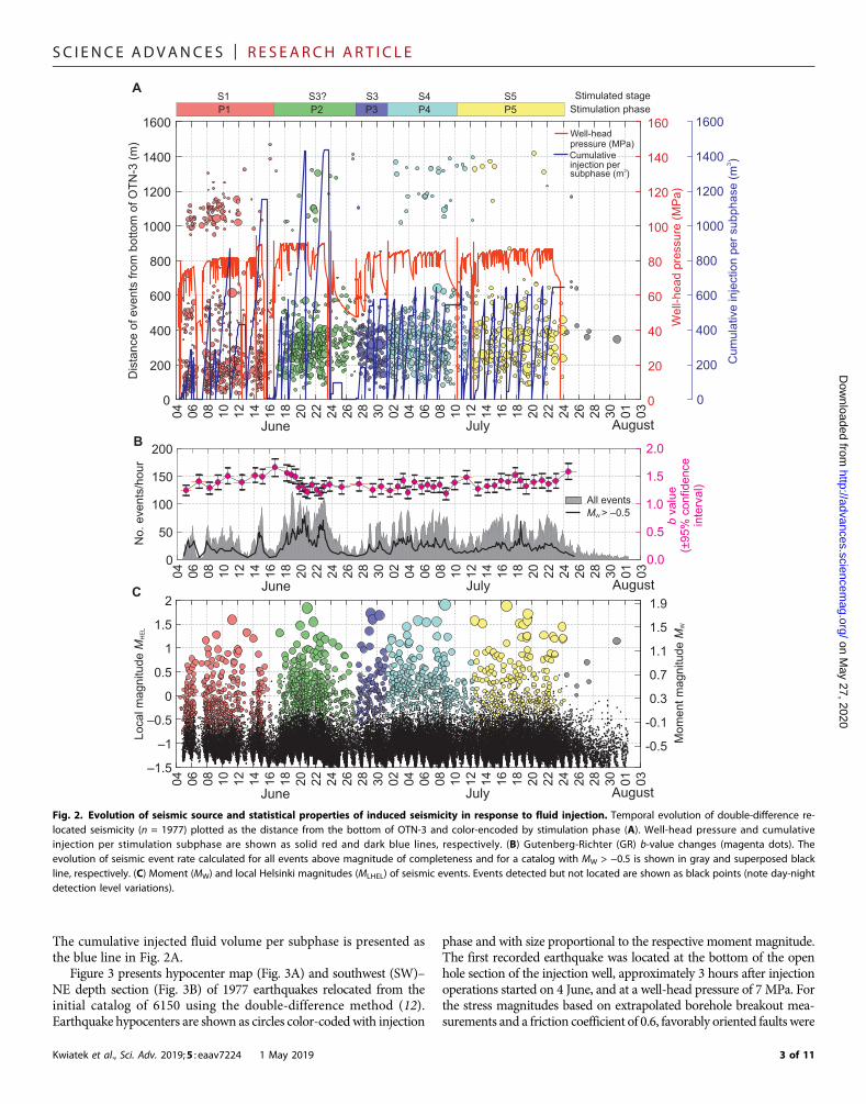
Figure 2A shows temporal changes in hydraulic and seismicparameters during the 49 days of injection and 9 days following shut-inof the well. Pumping was performed in five injection phases (P1 toP5 in Fig. 2A), each lasting 2 to 14 days. These phases were intendedto be pumped through corresponding stimulation stages S1 to S5 lo-cated along the open hole section of the OTN-3 well (Fig. 1, inset).However, the phase P2 stimulation was likely performed through thestage S3 port due to malfunctioning of the S2 port (for details, seeMaterials andMethods). Each phase consisted of multiple subphasesof continuous injection performed typically at a constant injectionrate, alternating with resting periods, when injection was stopped.

Fig. 1. Schematic view of the project site (see fig. S1 for a map view). The location of stimulation stages S1 to S5 into the bottom open hole section and basicstimulation parameters are shown in the inset.

2 of 11



on May 27, 2020


Dow

nloaded from

The cumulative injected fluid volume per subphase is presented asthe blue line in Fig. 2A.

Figure 3 presents hypocenter map (Fig. 3A) and southwest (SW)–NE depth section (Fig. 3B) of 1977 earthquakes relocated from theinitial catalog of 6150 using the double-difference method (12).Earthquake hypocenters are shown as circles color-codedwith injection


phase and with size proportional to the respective moment magnitude.The first recorded earthquake was located at the bottom of the openhole section of the injection well, approximately 3 hours after injectionoperations started on 4 June, and at a well-head pressure of 7 MPa. Forthe stress magnitudes based on extrapolated borehole breakout mea-surements and a friction coefficient of 0.6, favorably oriented faults were

–1.5

–1

–0.5

0

0.5

1

1.5

2

04 06 08 10 12 14 16 18 20 22 24 26 28 30 02 04 06 08 10 12 14 16 18 20 22 24 26 28 30 01 03

Loca

l mag

nitu

de M

HE

L

Mom

ent m

agni

tude

MW

-0.5

-0.1

0.3

0.7

1.1

1.5

1.9C

June July August

0

50

100

150

200

04 06 08 10 12 14 16 18 20 22 24 26 28 30 02 04 06 08 10 12 14 16 18 20 22 24 26 28 30 01 03

No.

eve

nts/

hour

0.0

0.5

1.0

1.5

2.0

b va

lue

(±95

% c

onfid

ence

in

terv

al)

All eventsMW > –0.5

B

June July August

0

20

40

60

80

100

120

140

160

04 06 08 10 12 14 16 18 20 22 24 26 28 30 02 04 06 08 10 12 14 16 18 20 22 24 26 28 30 01 03

June July August

pressure [MPa]pressure (MPa)

3subphase [m ]subphase (m3)

CumulativeCumulativeinjection perinjection per

Well headWell-head

Wel

l-hea

d pr

essu

re (M

Pa)

Dis

tanc

e of

eve

nts

from

bot

tom

of O

TN-3

(m)

0

200

400

600

800

1000

1200

1400

1600

Cum

ulat

ive

inje

ctio

n pe

r sub

phas

e (m

3 )

0

200

400

600

800

1000

1200

1400

1600P1 P2 P3 P4 P5

Stimulated stageStimulation phase

S1 S3? S3 S4 S5A

Fig. 2. Evolution of seismic source and statistical properties of induced seismicity in response to fluid injection. Temporal evolution of double-difference re-located seismicity (n = 1977) plotted as the distance from the bottom of OTN-3 and color-encoded by stimulation phase (A). Well-head pressure and cumulativeinjection per stimulation subphase are shown as solid red and dark blue lines, respectively. (B) Gutenberg-Richter (GR) b-value changes (magenta dots). Theevolution of seismic event rate calculated for all events above magnitude of completeness and for a catalog with MW > −0.5 is shown in gray and superposed blackline, respectively. (C) Moment (MW) and local Helsinki magnitudes (MLHEL) of seismic events. Events detected but not located are shown as black points (note day-nightdetection level variations).

3 of 11



on May 27, 2020


Dow

nloaded from

expected to be close to failure (13), with the consequent onset of seismicevents at a moderate fluid pressure increase (see Materials andMethods). Seismic activity increased substantially in the following6 hours of injection, starting once the well-head pressure exceeded70 MPa. No notable time delays between injection pressure, flow ratechanges, and the occurrence of seismicity were found during the entirestimulation (Fig. 2). There was also no evidence of Kaiser effect (14),where activity at a certain spot would start only after previous pressurelevels were exceeded.

A relatively quick dissipation of strain energy accumulated fromfluid injection is consistent with a sharp decrease in the seismic ac-tivity following shut-in phases (Fig. 2). Ultimately, 1 week after the finalshut-in of OTN-3 on 23 July, the hourly seismicity rate dropped from amaximum of 120 down to a few detected small events (Fig. 2B). Wealso noted that the seismic activity and seismic radiated energy releasecorrelated well in both time and magnitude with the product of in-jection rate and well-head pressure (=hydraulic energy EH). The seis-micity, and thus the seismic moment/seismic radiated energy release,was primarily sensitive to increases in the well-head pressure. Maintain-ing the well-head pressure and flow rate at 80 MPa and 400 liters/min,respectively, reduced the cumulative P1 seismic moment release to 50%of that observed in phases P2, P4, and P5. This is presented in Fig. 4A,which shows temporal changes in cumulative seismic moment for eachinjection phase. Similar low levels of seismicmoment release as in P1 didnot occur in the subsequent phases. Instead, phase P2 well-headpressures exceeding 90 MPa combined with longer and continuousperiods of pumping (Fig. 2A) accelerated the seismic moment/energyrelease rate (Fig. 4, A and B). This was manifested in a series of largerevents (up toMW = 1.8; Fig. 2C) that forced an end to P2.

OTN-3–induced seismicity showed a monotonic increase ofmaximum earthquake magnitude with the cumulative injected fluidvolume (Fig. 5). This increase followed the trend predicted by therecently introduced fracture mechanics–based model of Galis et al.


(10). It was also close to that presented by van der Elst et al. (15), butremaining much lower than the upper limit predicted by McGarr’s (8)model. According to Galis et al., this behavior suggests that the max-imum magnitude depends on both the regional tectonic stress and theimposed local fluid pressure controlling the total elastic energy storedin the system. Considering the observed trend in maximum magni-tude evolution with the injected fluid volume, it was expected thatthe MW 2.0 red alert threshold would likely be exceeded once the tar-geted fluid volume of 20,000 m3 was injected (note that the dashedline in Fig. 5 parameterized by g = 2 × 106 presents a post-stimulationassessment of the maximum magnitude evolution, with fluid volumeaccounting for actual reservoir and seismicity parameters). Therefore,following Galis et al.’s model, our pumping strategy was modified afterphase P2. Well-head pressures were limited to about 86 MPa (seemore detailed timeline in Materials and Methods). This pressure levelwas established by a trial-and-error procedure in an attempt to limitaccumulation of stored elastic energy due to injection and reach thetargeted cumulative injection volume. In a further adjustment to alsoreduce stored elastic strain energy by fluid pressure dissipation, theinjection subphases of P4 and P5 were reduced in duration to 18 hourswith 6-hour rest periods (see Fig. 2). As a final measure, pumping wasimmediately stopped and resting periods extended whenever a largeseismic event with MW > 1.7 occurred (Fig. 2).

These changes in the injection strategy after P2 were kept until theend of the stimulation. They seemingly stabilized seismic energy re-lease with respect to hydraulic energy in phases P3 to P5, although stillat a slightly higher release rate of radiated energy compared to P1(Fig. 4B). Equivalently, the seismic injection efficiency IE, the ratioof cumulative radiated energy to hydraulic energy EH (16), stabilizedafter P2 at a higher level (Fig. 4C). The flattening of IE suggested thatsome balance between strain energy buildup and dissipation hadbeen achieved, with IE only slightly increasing during the finalinjection phases. We believe that this approach allowed a successful

–1000 –800 –600 –400 –200 0 200 400 600Easting from OTN-3 bottom hole (m)

–1000

–800

–600

–400

–200

0

200

400

600N

orth

ing

from

OTN

-3 b

otto

m h

ole

(m)

Stimulation stage

Stimula

tion s

tage

–1000 –600 –200 200 600Distance along cross-section C-C' (m)

–6700

–6500

–6300

–6100

–5900

–5700

–5500

–5300

–5100

–4900

–4700

Alti

tude

(m)

Stimulation stage

OTN-2OTN-3

OTN-3

C

C'

P1 P2 P3 P4 P5

NStimulation phase

Cross-s

ectio

n C-C

'

ST1 Deep Heat

S1S2

S3

S4

S5

S1

S1

S2

S2

S3

S3

S4

S4

S5

S5

C C'

maxSH

N110°E

A B

P1 P2 P3 P4 P5

Stimulation phase

MW

2.01.00.3

–0.5

MW

2.01.00.3

–0.5

Fig. 3. Induced seismicity hypocenters during stimulation campaign. (A) Map view and (B) SW-NE depth section showing double-difference relocated seismicity(n = 1977) color-coded with stimulation phase. Injection stages S1 to S5 are colored accordingly from the bottom of the open hole (6.4 km MD) toward the casingshoe (5.4 km MD) of OTN-3. The size of each event is proportional to the moment magnitude.

4 of 11



on May 27, 2020


Dow

nloaded from

completion of the stimulation plan while avoiding a project derailingMW > 2.0 red alert induced earthquake.

Upon completion of injection, the seismic data were reprocessedto further reduce the magnitude detection threshold and to refineearthquake source parameters. This aimed at improving our under-


standing of the spatial and temporal development of induced seismicity,and investigates factors leading to observed behavior of maximummagnitude. This reprocessing (see Materials and Methods) enlargedthe original near–real-time industrial seismic catalog to 43,882events, with magnitudes down to MW = −0.6. From this extendedcatalog, all events withMW > 0.7 were manually reviewed. A furthersubset of 1977 best-recorded earthquakes that occurred in the imme-diate vicinity to the injection well (Fig. 3) was relocated using thedouble-difference relocation method (12). This improved the rela-tive hypocenter precision down to ~27 and ~66 m for 68 and 95%,respectively, of the relocated catalog.

DISCUSSIONThe induced seismicity occurred in three main spatially separatedclusters located along the injection interval of OTN-3 (Fig. 3). Theclusters were active simultaneously but showedno clear spatial or tem-poral links to the injection ports opened during specific stimulationstages. An additional small fourth cluster located near the upperend of the open hole was developed during the last injection phases(P4 and P5). These and other engineering observations including largecaliper logged along the open hole section suggest that the injectedfluid might pass along the damaged wall rock of the OTN-3 well, by-passing the stage packers.

The events within each cluster trended and expanded in the south-east (SE)–northwest (NW) direction as stimulation progressed. This di-rection is subparallel to the direction of maximum horizontal stress(SH

max) (13) and coincides with surface features mapped in the vicinityof the project site (17). The upper two main clusters roughly correlate

0

1

2

3

4

I eff

(×10

–3)

P1P2

P3 P4 P5

06/0

306

/07

06/1

106

/15

06/1

906

/23

06/2

707

/01

07/0

507

/09

07/1

307

/17

07/2

107

/25

07/2

908

/02

08/0

6

Date

0 0.5 1 1.5 2Hydraulic energy (J × 1012)

0

1

2

3

4

5

6

Cum

ulat

ive

radi

ated

ene

rgy

(J ×

109 ) P1P1

P2P2P3P3P4P4P5P5

Stimulation phaseStimulation phase

0 2 4 6 8 10 12Time since beginning of injection phase (days)

0

2

4

6

8

10

12

14C

umul

ativ

e se

ism

ic m

omen

t (×1

012 N

m)

P1P1P2P2P3P3P4P4P5P5

Stimulation phaseStimulation phase

A

B

C

Fig. 4. Evolution of seismic moment, radiated energy and hydraulic energyrelease during stimulation. (A) Cumulative seismic moment release with time.(B) Cumulative radiated seismic energy release as a function of hydraulic energy.(C) Seismic injection efficiency IE changes with time.

102 103 104 105 106

Cumulative volume injected (m3)

0

1

2

3

4

5

Max

imum

obs

erve

d m

omen

t mag

nitu

de

1010

1110

1210

1310

1410

1510

1610

Max

imum

obs

erve

d se

ism

ic m

omen

t (N

m)

BER BER

NBY NBY BSH BSH

KTB KTB

BUK BUK

GAR GAR

BAS BAS

CBN CBN

STZ STZ

ASH ASH

YOH YOH ASH ASH

RAT RAT GAK GAK RMA RMA

Enhanced Geothermal Systems

Hydrothermal reservoirs

Scientific

BAS - Basel (Switzerland)CBN - Cooper Basin (Australia)STZ - Soultz-sous-Forets (France)

BER - Berl n (El Salvador)NBY - Newberry EGS (USA)

KTB - Ultradeep well (Germany)

í

Enhanced Geothermal SystemsBAS - Basel (Switzerland)CBN - Cooper Basin (Australia)STZ - Soultz-sous-Forets (France)Hydrothermal reservoirsBER - Berlín (El Salvador)NBY - Newberry EGS (USA)ScientificKTB - Ultradeep well (Germany)

Wastewater disposal

Fracking

ASH - Ashtabula (USA)GAK - Guy (USA)RAT - Raton basin (USA)RMA - Denver (USA)YOH - Youngstown (USA)

BUK - Bowland Shale (UK)GAR - Garvin County (USA)

Wastewater disposalASH - Ashtabula (USA)GAK - Guy (USA)RAT - Raton basin (USA)RMA - Denver (USA)YOH - Youngstown (USA)FrackingBUK - Bowland Shale (UK)GAR - Garvin County (USA)

P1P1P2P2

P3P3

P4P4

P5P5

McGarr (b = 1.3)

McGarr (b = 1.3)

1010

0.10.1

van der Elst

van der Elst

= –2.8= –2.8

= –0.8= –0.8

= –1.8= –1.8

Fig. 5. Temporal evolution of maximum observed seismic moment versuscumulative volume of injected fluid at each phase (P1 to P5). Colored circlesare from various injection projects (8, 19, 20). Maximum magnitude estimatesusing different models are shown with solid, dashed, and dotted lines (8, 10, 15).The g and b parameter values used in (8, 10) were calculated after the stimulation,assuming geomechanical and seismic parameters from this study, and plotted forcomparison with the observed evolution of seismic moment (see Materials andMethods).

5 of 11



on May 27, 2020


Dow

nloaded from

with locations where drilling progress was difficult, including a drillstring jammed at the beginning of inclined section OTN-3 while thewell was drilled, and small fluid losses observed in this area. In addition,anomalies in well logs including temperature fluctuations, caliper logs,and higher density of borehole breakouts were encountered in these in-tervals, suggesting the existence of discrete, broad damage zones. It isthen likely that fluids propagating along the damaged wall rock of theOTN-3 well, beyond the stimulation tool, were entering all damagezones concurrently, regardless of the active injection stage. The spatiallylargest hypocenter cluster occurred at and below the bottom of OTN-3.It was active throughout the whole stimulation, with seismicity slow-ly deepening with time toward the NE.

Source sizes calculated for 56 events with MW > 1.1 using spectralanalysis (seeMaterials andMethods) display source radii of 11 to 34m,assuming circular source model of Madariaga (18). Combined withestimated hypocenter precision and spatial extent of clusters, this in-dicates that the hypocenter cloud shows no evidence for alignmentalong a large fault, but rather appears as the activation of a broadnetwork of distributed fractures. Moreover, a significant drop-offin the number of events aboveMW>1.5 exists in theGutenberg-Richter(GR) distribution of the induced earthquakes (fig. S4). Hence, thestimulated volume may not contain faults large enough to sustainlarger events. Alternatively, the fluid injection did not store enoughelastic energy in the reservoir to support a runaway rupture on alarge fault (10).

The activation of a distributed fracture network is supported bycomparison of empirical data of seismic injection efficiency IE fromvarious sites. For St1, the observed values of IE ranges from 2.0 × 10−3

in P1 to 3.2 × 10−3 in P5 (Fig. 4C). This range of values is higher thanthe IE < 10−5 commonly reported for hydraulic fracturing campaigns,where new fractures are being created (19–21). It is, however, lowerthan the IE reported for the EGS stimulations at Basel and CooperBasin (19), where IE ranged between 10−2 and 1. This is expected,as maximum magnitudes at these sites were also larger (Fig. 5): 3.4at Basel and 3.7 at Cooper Basin (22, 23). At Basel and Cooper Basin,nearby larger faults were apparently activated. Combined, the low IEvalues during OTN-3 stimulation, the clustering of event locations inbroad zones, and the statistically significant breakdown of GR b valueat large magnitudes would suggest that the OTN-3 stimulation acti-vated a preexisting small-scale fracture network rather than a promi-nent, single, large fault.

The catalog of 43,882 induced earthquakes covering the stimula-tion period and 1 week after the stimulation indicates that betweenthe GR b value increased in phase P1 from 1.2 to 1.6 (Fig. 2B). Thismay correspond to the reactivation/creation fracture network at thebeginning of injection. However, the b value returned to and then re-mained at ~1.3 during the subsequent stimulation phases P2 to P5.Thus, the earthquake hazard correlated primarily with the seismicactivity—the GR a value (see Fig. 2B)—rather than the ratio of smallto large events, the GR b value.

Presumably, tectonic loading rates at the St1 site are lower com-pared to other sites located close to active faults (e.g., as in the RhineGraben/Basel and close to the Alps). If the temporal changes in b val-ue are a function of the mean crustal stress evolution as proposed byothers (24), then our observations suggest that the OTN-3 stimulationdid not lead to a notable and persistent increase in deviatoric stressesduring later injection phases. This is different from the observations atthe Basel EGS site, where b values have been observed to decrease (25)with progressing injection, likely associated with a long-lasting stress


perturbation. In addition, the observed seismicity shows no substantialspatial clustering in rescaled interevent times and distances (fig. S5) (26),indicating minor earthquake interaction/triggering and low stresstransfer (27). This suggests that stress changes induced by theOTN-3 stimulation may have been quickly relaxed by the small-scaleseismic activity along weak fractured zones.

For critically stressed rock, small pore pressure changes are suffi-cient to activate favorably oriented faults and fractures, as observed inthis and similar stimulation projects. Our observations suggest thatfluid injection activated a network of preexisting faults and fractures.In particular, the located seismic activity indicated growth of three-dimensional (3D) ellipsoidal event clusters rather than activation of aprominent fault structure. We observed that maximum induced-earthquake magnitudes scaled with the injected fluid volume closelyfollowing a trend predicted by a fracture mechanics–based model(10), which relates maximum magnitudes of self-arrested earthquakesto the injected fluid volume.We adjusted the injection rates in an effortto constrain the amount of stored elastic energy available for rupturepropagation, maintaining a low ratio of radiated energy to hydraulicenergy input. This was achieved in an iterative procedure by reducinginjection rates and extending waiting periods between pumping phases.Adjusting the stimulation schedule to the observed evolution of inducedseismicity allowed us to successfully prevent the occurrence of largerevents exceeding a TLS-defined red alert. It is possible that the advan-tageous geological and tectonic reservoir features and favorable stress(transfer) conditions contributed to project success, although theirdetailed role needs to be further investigated. We expect that differenttectonic settings and geological boundary conditionswould require spe-cific adjustments of injection schedules.

Controlling injection-induced seismicity is of crucial importancefor public acceptance of enhanced geothermal energy projects. Thetwo cases of EGS in Basel (2, 3) and Pohang (4, 5) showed a broadnegative socioeconomic impact of EGS-associated seismicity, even re-gardless of whether, in the latter case of Pohang, the causal relationbetween EGS operations and the occurrence of large event is a subjectof pending investigation. This negatively affects the support of com-munities to geothermal energy, as well as increases the economic costsof EGS implementation due to the enhanced risk.

In St1 project at the Aalto University campus, we used near–real-time seismic monitoring to modify stimulation parameters to success-fully limit induced-earthquake magnitudes to the maximum allowableMW = 2.0. This result was achieved by close cooperation of seismol-ogists, site operator, TLS teams, and local authorities during the stim-ulation operation.

MATERIALS AND METHODSSite descriptionThe St1 drill site is located on crystalline Precambrian Svecofennianbasement rocks. These are only locally covered by 20 m or less ofquaternary glacial deposits and clay-rich soils. They represent a deepcrustal section of deformed metamorphic and intrusive granites, peg-matites, quartzo-feldspathic gneisses, and amphibolites (28). In thecourse of post-Precambrian tectonics, Late Mesozoic plate motions,and Holocene glacial rebound, the basement rocks became folded, fo-liated, jointed, and faulted.

On the basis of inversion of regional earthquake focal mechanisms,the current local maximum horizontal stress is oriented N110°E (29).Roughly normal to this and ~8 km to the NW of the drill site is the

6 of 11



on May 27, 2020


Dow

nloaded from

~50-km-long, left-lateral Porkkala-Mäntsälä fault zone (30). Thelargest instrumentally recorded earthquake on this fault was anM2.6 event in 2011 (31). About 1.5 km to the SE is a similarly orientedand long, but apparently inactive, thrust fault, likely dipping to the SE(17). Drill bit seismic data recorded at the site suggest that an addi-tional SE to SW 70° to 80° dipping structure 1 to 2 km to the NWmayintersect the injection well at depths of 5.4 to 6.2 km. The closestknown earthquakes to the drill site were MW 1.7 and MW 1.4 events,recorded in 2013 (31).

Stress magnitudes at the drill site were estimated from wellborebreakouts and minifrac shut-in pressures measured down to a depthof 1.8 km (13). Extrapolated to a depth of 6.1 km, these were estimatedto be SH

min = 110 MPa, SV = 180 MPa, and SHmax = 240 MPa. Pore

pressures were assumed to be hydrostatic, equaling to approximately60 MPa. Assuming a friction coefficient of 0.6, these results suggestedthat optimally oriented fractures and faults could be readily activatedwith moderate fluid pressure increases.

Seismic networkThe real-time telemetered network monitoring the stimulation cam-paign was composed of 24 borehole seismographs, fabricated,installed, and operated by Advanced Seismic Instrumentation and Re-search (www.asirseismic.com; fig. S1). The 12-level borehole array ofthree-component 15-Hz natural frequency Geospace OMNI-2400geophones was sampled at 2 kHz. This array was placed at depthsof 2.20 to 2.65 km in the OTN-2 well. Additional 12-station three-component fN = 4.5 Hz Sunfull PSH geophones sampled at 500 Hzwere installed in 0.30- to 1.15-km-deep wells. These surrounded theproject site at 0.6- to 8.2-km epicentral distances. These two networkswere operating months before the start of stimulation with no event.Last, a 14-station ground motion network was placed at critical surfacesites in the Helsinki area to monitor the ground motions for the pur-pose of TLS operation. This network was not used in automated near–real-time processing discussed after the following section.

Traffic light systemThe TLS consisted of green, amber, and red thresholds, where ex-ceedances of an amber threshold required notifications to be com-municated and additional analyses to be performed; exceedances ofa red threshold additionally required stimulation activities to be stoppedas quickly as safely possible. The selection of thresholds was based onPGV thresholds and their impacts on the population and the builtenvironment. These PGV thresholds were then translated into magni-tude thresholds using both global (32) and local (33, 34) groundmotionprediction equations (GMPEs). More specifically, magnitudes asso-ciated with PGV thresholds were selected on the basis of a conservative-ly low probability (i.e., either 10 or 2%) that the seismic event wouldresult in a PGVat the surface sufficient to cause aTLS exceedance, basedon the GMPE uncertainties. Implemented TLS thresholds were basedon either exceeding both a PGV and local “Helsinki”magnitude,MLHEL

(33, 34), or a separate scenario where only a magnitude was exceeded.The formerwas developed to confirm thatmonitored surface vibrationswere related to seismic events, while the latter was developed in theevent that an unacceptable surface expression would occur in an areaabsent of surface monitoring.

Automated near–real-time seismic catalogDuring the injection campaign, a seismic catalog was created in nearreal time and used for traffic light operations. Thewaveformdata from


sensors located in the OTN-2 well (three sensors—OT06, OT11, andOT12—with the largest noise levels were not used in the online pro-cessing) and satellite borehole stations were analyzed by using fullyautomated fastloc.REEL software (fastloc GmbH; www.fastloc.eu)and by providing an automated hypocenter location and magnitudeestimate. The P-wave onsets were detected using a STA/LTAcharacteristic function. The location procedure was triggered whenthe timely order and timely proximity ofminimumnine P-wave arriv-als indicated that an event occurred at any depth within a 5-km cyl-inder around the inclined portion of theOTN-3well. Events occurringwithin these spatial limits were all passed to the TLS operator (see thenext section).

The modified equivalent differential time (EDT) method (20, 35)was used to locate each earthquake individually using 1D velocitymodel compiled from the borehole logs performed in OTN-1 andOTN-3 wells, regional information on P- and S-wave velocities, andVP/VS ratio (fig. S2). The location inverse problem was solved usingthe global search adaptive simulated annealing (36) algorithm. The lo-cal magnitudeMLHEL required by TLS was calculated from maximumamplitudes of the three-component seismograms (33). This automat-ically calculated hypocenter location and local magnitude estimateswere available to the TLS operator and the stimulation engineers typ-ically within <5 min since earthquake occurrence. The information onearthquake source parameters was concurrently forwarded via mobilephones to all parties involved in the project using a notification appand included in a dedicated web page.

On completion of stimulation, the catalog contained 8452 eventdetections overall, and 6152 confirmed earthquakes located in thevicinity of the project site (epicentral distance from the well headof OTN-3, <5 km). These were recorded in a time period lasting59 days: 49 days of active stimulation campaign and 10 days followingthe shut-in.

TLS and stimulation operationsFollowing the TLS established for this project, all larger seismic eventswith MLHEL > 1.1 (MW = 1.2) needed to be reported to local author-ities within 20 min. Events of this size and up to a limit of MLHEL =2.1 (MW = 2.0) were allowed without further consultation. Above theupper limit, a TLS red condition existed and no further injection wasallowed without new approvals from the Finnish government.

Hence, it was decided to manually reprocess allMW > 1.1 to ensureaccuracy before the mandated reporting. If necessary, the reprocessingincluded manual review and repicking of P- and S-wave arrivals bythe seismic team operating on a 24/7 schedule. This was followedby relocation of the event and reestimation of the magnitude. Themanual review procedure typically lasted for an additional 10 min af-ter initial information produced by the processing software. Updatedsource parameters of reprocessed events were communicated as forautomatic processing to TLS and stimulation engineers. This required5 to 15 min, on average, until automatic and revised source character-istics were available, respectively. The initial and eventually the revisedsource information (the latter on MW > 1.1 earthquakes) was for-warded to the TLS operator. The TLS operator provided continuousfeedback to stimulation engineers (whenever a non-green TLS condi-tion occurred), accounting for information on earthquake rates providedby the seismic team and PGV information recorded using the groundmotion network (fig. S1). This feedback was used by the injection en-gineers to modify the injection rate during the experiment. Some keytime intervals and actions taken to control the seismicity within TLS

7 of 11

http://www.asirseismic.com

http://www.fastloc.eu



on May 27, 2020


Dow

nloaded from

limits are presented in the next section and indicated in fig. S3 usingRoman numerals.

Apart from near–real-time processing and immediate forwarding ofinformation, the response of the seismicity (such as event rate, radiatedenergy, and maximum magnitude) due to changes in the pumpingparameters was analyzed in retrospect and discussed between the seis-mic team, TLS operator, and stimulation engineers. For example, theinsight gained especially in phases P1 to P3 on maximum magnitudedevelopment with respect to the injected fluid volume was used tooptimize well-head pressures and flow rates, as well as the durationof waiting periods for the following pumping stages. This resulted atthe end-of-June and mid-July changes in the pumping proceduresevident in fig. S3. If the stimulation would have been continued fur-ther, then additional changes in the seismicity-pumping protocolwould have been implemented using this additional feedback sys-tem. However, this did not become necessary as the engineering tar-get for the net volume was achieved before.

StimulationStimulation phases P1 to P5 (Fig. 2) were planned to be performedthrough five frac ports into the corresponding stages S1 to S5. Allports were located along the open hole section of the OTN-3 well(Fig. 3). These were opened sequentially using gauge-controlledmagnesium sealing spheres pumped to the ports at specific pressures.However, the sealing pressure data and a seismicity-inducing pressurepulse test performed after phase P1 suggested that, during phase P2,fluids were entering the formation in the interval of S3. The engineer-ing data for phases P4 and P5 subsequently confirmed opening of S4and S5, as expected.

A total amount of 18,538 m3 of fresh water was injected into stagesS1 to S5. The total amount of backflow was 378 m3, leading to18,160 m3 resident in the stimulated formation. The stimulation plansincluded pump tests at the beginning and end of each stimulationphase (P1 to P5). The initial stimulation in P1 reached an injectionpressure of over 80 MPa and led to seismicity close to the injectionwell in the main three clusters in Fig. 3. In phase P2, the pressureswere increased to over 90 MPa, and the last two stimulation subphaseswere performed over a couple of days without any resting periods (I infig. S3). This resulted in a significant increase of seismic activity, most-ly occurring in the bottom cluster (Figs. 2 and 3) and accelerated seis-mic moment release (Fig. 4B). The activity also expanded toward theNE, along a SE-NW axis, and went to greater depths. Phase P2 con-cluded with the occurrence of larger seismic events. At this moment,two observations were notable: (i) The observed maximum magnitudeafter phase P2 was significantly below the upper limit predicted byMcGarr’s (8) model, and (ii) the evolution of maximum magnitudeappeared to follow the behavior predicted by a recently publishedmodel of Galis et al. (10) (see Fig. 5). Accounting for these observa-tions, it was a concern of the St1 project team that injecting theintended fluid volume of 20,000 m3 could potentially cause a red alertMW 2.0 event. To this end, we adjusted the injection rates in an effortto constrain the amount of stored elastic energy available for rupturepropagation by maintaining a low ratio of radiated energy to hydraulicenergy input. This was achieved in an iterative procedure by reducingflow rates and extending waiting periods between pumping cycles. Forthis reason, stimulation was first stopped for over 4 days (II in fig. S3),with the aim of at least partially releasing the already accumulated hy-draulic energy. Ahead of stage P3, a pulse test was performed to con-firm that the P1-P2 pumping was exiting through stage S3. In phase


P3, the stimulation was performed at injection pressures less than90 MPa (III in fig. S3) to reduce the rate of hydraulic energy input intothe rock mass and, consequently, to reduce the accelerating seismicmoment release observed in phase P2 (see Fig. 4, A and B).

The seismicity in P3 continues to appear mostly in the bottom-most cluster. However, the seismic moment release linearizes with hy-draulic energy (see Fig. 4, A and B). Nevertheless, during phase P3,larger events occurred, leading to a further change in the injectionstrategy. Phases P4 and P5 were performed at similar pressures, butfor limited time intervals, typically composed of 12 to 18 hours ofinjection followed by 6 to 12 hours of resting period (IV and V infig. S3). Again, this aimed at decreasing the stored amount of elasticenergy in the system, now by extending waiting periods to allow thefluid pressure in the reservoir to dissipate. Moreover, when furtherincreases in seismic activity and occurrence of larger seismic eventswere observed, these were used to justify even earlier shut-in and longerresting periods. These strategies stabilized seismic injection efficiency(Fig. 4C) that will not increase substantially anymore until the end ofinjection. The largest seismic event (MW = 1.90) occurs in the bottomcluster and triggers the completion of injection phase P4. However, theseismicity from this phase and the following P5 is generally comparable.The main bottom cluster is further expanding in depth, to NE, andalong the SE-NW azimuth. The remaining two main clusters becomeoverall more active, expanding toward SE andNW. Thismay be relatedto the fact that stimulation stages were now located closer to theseclusters, leading to higher local stress perturbation despite overall lowerinjection pressures.

The stimulation was finalized successfully after 49 days. In the sub-sequent 10 days, the seismicity level reduced to a few detectable eventsper hour. During this period, three events with amber magnitudes (allMW ≅ 1.3) occurred in the first few hours after the shut-in.

Industrial catalog postprocessing and refinementThe initial industrial seismic catalog of 6150 earthquakes was man-ually reprocessed. The P- and S-wave arrivals of seismic events withMW > 0.7 were all manually verified and, if necessary, refined. Earth-quakes with sufficient number of phases and seemingly anomaloushypocenter depths (e.g., very shallow or very deep) were also manuallyrevised.

The hypocenter locations were calculated using the EDT method(20, 35) and an adaptive simulated annealing optimization algorithm(36), using a modified velocity model (fig. S2) with an optimized VP/VS

ratio and slightly increasedVP at larger depths. TheVP/VS = 1.68 andVP that minimized the sum of location root mean square error un-certainties was selected for the final hypocenter determinationprocedure. This value is close to that reported for the crust at a depthof 10 km in theHelsinki area. The updated catalog contained 4580 earth-quakes that occurred at hypocenter depths of 4.5 to 7.0 km, in the vi-cinity of the stimulation section of OTN-3.

To increase the precision of their locations, we selected 2155 earth-quakes with at least 10 P-wave and 4 S-wave picks and relocated themusing the double-difference relocation technique (12). The relocationuncertainties were estimated using the bootstrap resampling technique(12). The relocation reduced the relative precision of hypocenter de-termination (2s) to approximately 66 and 27 m for 95 and 68% ofrelocated earthquakes, respectively. This enabled tracing the spatialand temporal evolution of seismicity in much greater detail. Thedetailed catalog contained 1977 earthquakes (91% of the originallyselected events).

8 of 11



on May 27, 2020


Dow

nloaded from

Industrial catalog extension to smaller magnitudesUnused P-wave arrivals detected using the array located in OTN-2were also analyzed further. Assuming that a small event that is de-tected solely at the OTN-2 array must occur in its immediate vicinity,we placed a hypothetical seismic source at the bottom of OTN-3. Inthe following, we calculated travel times of P waves to the sensorsforming theOTN-2 array, thus obtaining a particular pattern of P-wavearrivals.We then scanned the catalog of unusedOTN-2 P-wave arrivalsfor this particular pattern, and each matching set of detections wasattributed to an event occurring in the vicinity of the OTN-3 well. Wethen calculated itsmagnitude by assuming that it occurred at the bottomof theOTN-3 injection well. This simple yet effective procedure allowedus to enhance the catalog by ~54,000 earthquakes withMW ≤ 0.1.

Statistical and clustering propertiesThe b value for the OTN-3 seismicity was calculated for the initialcatalog extended to smaller magnitudes using the goodness-of-fitmethod (37), using Aki-Utsu formula and correction for magnituderounding (38). The calculation was completed assuming that 95%of events are explained by a GR power law. This resulted in b = 1.26with 2s = 0.02 and an estimated local magnitude of completenessof MC = −1.21. The final catalog of events above this magnitudethreshold contains 43,882 earthquakes (fig. S4). However, it shouldbe noted that the number of earthquakes below MLHEL= −1.0 (MW ≅−0.5) varied with time of day, with a bias toward low-noise night times(Fig. 2C). Thus, it is more likely thatMLHEL ≅ −1.0 (MW ≅ −0.5) is theuniform, time-independent detection limit of the 24-station network,with 25,378 earthquakes above this limit.

Temporal changes in the b valuewere calculated from the subcatalogof 25,378 earthquakes withMLHEL≥ −1.0. This was done using a roll-ing window of 400 events (different windows of 300 and 500 magni-tudes have also been tested). The resulting temporal sequence ofn= 50b values, [bi] (Fig. 2B), was tested for stationarity using the augmentedDickey-Fuller (ADF) test (39). It was identified that the initial 12b values [bi]i=1…12, corresponding to the stimulation phase P1, forma nonstationary series (Fig. 2B) of increasing b values. However, forthe remaining sequence [bi]i=13…50, corresponding to phases P2 toP5, the ADF null hypothesis that the b-value time series has sometime-dependent component was rejected at 99% confidence intervals(P < 10−4).

To test whether the drop-off in a number of events above MW 1.5(fig. S4) is an actual feature, and not accidental due to the limited datasample, we used the smoothed bootstrap test for multimodality(40, 41) and the nonparametric approximation of GR relation (38, 42).Similarly to temporal variations in b value, we used the catalog con-strained toMLHEL ≥ −1.0 to remove the effect of day-night noise cycle.The significance of the null hypothesis that the number of bumpsabove the magnitude of completeness in magnitude density equals1 is very low (P < 0.01), meaning that the magnitude population hasa two-component structure. As expected, the change in inclination ofGR distribution was found around MW 1.5.

The updated catalog of 4580 near-well events with depths between4.5 and 7.0 km was analyzed in terms of its clustering properties. Wefollowed the well-established, scale-free, space-time-magnitude nearest-neighbor proximity technique (26, 43). This method looks for violationof the null hypothesis that earthquakes in the selected catalog occurrandomly with a rate given by the GR relation (27). The separationbetween background seismicity and triggered earthquakes (after-shocks) is identified using distribution of rescaled interevent times


and distances. In the absence of triggering, this distribution tendsto be unimodal. Overall, it would thus be comparable to one createdby a randomized version of the target catalog (27). In the latter case,magnitudes and event origin times appear independent. However,clustered/triggered earthquakes form additional modes in the distri-bution with typically shorter interevent times and distances. This seis-micity can be recognized manually by setting a separation thresholdwith the help of the reshuffled catalog (27), whichwas used in this study.Alternatively, clustered/triggered seismicity can be extracted using amixture Gaussian model (44, 45), leading to comparable results.

In this analysis, we assumed b = 1.26 and a fractal dimension d =1.41, the latter estimated using the box-counting method. The rescaledtime difference–to–distance difference plot does not display a clearmultimodality (fig. S5A). Therefore, we calculated the distributionusing the reshuffled catalog and selected the threshold level manually(fig. S5B). The result is that practically all induced seismic activityfrom the OTN-3 stimulation can be considered as background seis-micity, imposing that the selected catalog does not show the signaturesof clustering/triggering.

Source parameter estimationCatalog local magnitude MHEL calculated following Uski et al. (34)was converted to seismic moment M0 using the formula M0 ¼10ððMLHELþ7:98Þ=0:83Þ(34), which provides reliable moment estimatesfor small earthquakes with local magnitudeMLHEL > 0.6. This was thenrecalculated to moment magnitude using the standard relation (46)

MW ¼ ðlog10M0 � 9:1Þ=1:5 ð1Þ

To calculate radiated energy, we used (46)

E0 ¼ DsM0

2Gð2Þ

where Ds is the static stress drop and G is the shear modulus. We as-sumed shear modulusG = rVS

2 = 39.2 GPa, where r = 2700 kg m3 andVS = 3810m s−1, the density and velocity at the bottom of the open holesection of OTN-3, respectively (see fig. S2).

To calculate the stress drop, we performed spectral analysis of56 largest events with MW > 1.1 that were well recorded on shallowborehole sensors. The here described procedure follows the spectralfitting approach (47–49). The three-component seismograms werefirst filtered using a 1-Hz high-pass Butterworth filter and then in-tegrated to obtain the ground displacement waveforms. The P andS waves were analyzed using a time window of 0.512 s length starting0.016 s before P- or S-wave onsets. The windows were smoothed usingvon Hann’s taper, and ground displacement spectra were calculatedfrom all components using the multitaper method (50) and then com-bined together. The observed ground displacement spectra were fit toBoatwright’s point-source model (51)

uð f ;M0; f 0;QCÞ ¼RC

4prVC3RM0

ð1þ ð f =f 0Þ4Þ0:5exp � pf R

QCVC

� �ð3Þ

where R is the source-receiver distance, M0 is the seismic moment,f0 is the corner frequency, QC is the quality factor, and RC is the av-erage radiation pattern correction coefficient. We used RP = 0.52

9 of 11



on May 27, 2020


Dow

nloaded from

and RS = 0.63 for P and S waves, respectively (52). We assumed VP =6390 m s−1 and VS = 3810 m s−1. For each station and phase, weinverted for [M0, f0, QC] optimizing the cost function L2 norm be-tween the observed and modeled spectrum. The initial model wasselected using Snoke’s integrals (53) and grid search techniques. Thiswas followed by optimization of the cost function following the globalcoyote optimization technique (54). The stress drop was calculatedusing Eshelby’s equation (55)

Ds ¼ 716

M0

r03ð4Þ

where r0 is the source radius calculated from corner frequency,assuming circular source model

r0 ¼ cVC

2pf 0ð5Þ

where c is constant depending on the assumed source model. Assum-ing Brune’s source, the median stress drop of analyzed earthquakes is1.6 MPa, whereas assuming the Madariaga source model (18) led to amedian value of 8.7 MPa. Figure S6 presents the relation betweencorner frequency and seismic moment for analyzed earthquakes, withcontours of constant static stress drop assuming a Madariaga model ofthe source radius. The resolved stress drops are in a similar range asreported in other studies on induced seismicity (49), as well as naturalearthquakes within the investigated magnitude range. We arbitrarilyselected a Madariaga model–based median estimate of the static stressdrop (Ds = 8.7 MPa) to recalculate seismic moments of analyzedearthquakes to radiated energy following Eq. 2.

Hydraulic energy and seismic injection efficiencyThe hydraulic energy in any arbitrary time interval [t1, t2] wascalculated as

EH ¼ ∫t2

t1PðtÞVðtÞdt ð6Þ

where P and V are measured well-head pressures and injection rates,respectively. The seismic injection efficiency (16, 21) IE in time interval[t1, t2] was calculated as the ratio of cumulative radiated energy ofearthquakes that occurred in a specified time period and hydraulicenergy EH (t1, t2).

Calculation g parameter of Galis et al.In the model of Galis et al. (10), the maximum moment magnitudeof arrested rupture depends on the injected fluid volume as in

Mmax0 ¼ gDV3=2 ð7Þ

where g parameterized as

g ¼ 0:4255ffiffiffiffiffiffiDs

p kmdh

� �3=2

ð8Þ


Although the formula contains a number of poorly known param-eters, it is interesting to assess the difference between the maximummagnitude defined by Galis et al. and actual observations. For the cal-culation of g, we used median static stress drop Ds = 8.7 MPa esti-mated in the course of spectral analysis, a bulk modulus of 58.1 GPa, adynamic friction coefficient of 0.1, and reservoir thickness h = 1000 m.The bulk modulus was calculated using k = l + 2G/3, where l =r(VP

2 − 2VS2) is the Lame’s first parameter, r = 2700 kg m−3, VP =

6390 m s−1, and VS = 3810 m s−1. As a representative reservoirthickness, we selected the approximate size of all clusters altogether.The dynamic friction coefficient was identical to that used by Galis et al.This resulted in g = 2.0 × 106, which is close to the observed trend ofmaximum magnitude evolution shown in Fig. 5.

SUPPLEMENTARY MATERIALSSupplementary material for this article is available at http://advances.sciencemag.org/cgi/content/full/5/5/eaav7224/DC1Fig. S1. Location of St1 Deep Heat Oy project site and different seismic networks used tomonitor the stimulation campaign.Fig. S2. Optimized velocity model for P and S waves (black and red lines, respectively), initiallycompiled from borehole logs.Fig. S3. Key time intervals indicating changes in pumping protocols (Roman numerals)together with pressure and cumulative injection per injection subphase (see Materials andMethods for detailed description of changes in pumping protocol).Fig. S4. b-value distribution for the full catalog.Fig. S5. Results of declustering analysis.Fig. S6. Dependence between corner frequency and seismic moment for the group of 56earthquakes with MW between 0.9 and 1.9, for which spectral parameters have been estimatedusing the spectral fitting method.Text S1. Access to catalog data

REFERENCES AND NOTES1. W. L. Ellsworth, Injection-induced earthquakes. Science 341, 1225942 (2013).2. D. Giardini, Geothermal quake risks must be faced. Nature 462, 848–849 (2009).3. T. Diehl, T. Kraft, E. Kissling, S. Wiemer, The induced earthquake sequence related to the

St. Gallen deep geothermal project (Switzerland): Fault reactivation and fluid interactionsimaged by microseismicity. J. Geophys. Res. Solid Earth 122, 7272–7290 (2017).

4. K.-H. Kim, J.-H. Ree, Y. Kim, S. Kim, S. Y. Kang, W. Seo, Assessing whether the 2017 Mw 5.4Pohang earthquake in South Korea was an induced event. Science 360, 1007–1009(2018).

5. F. Grigoli, S. Cesca, A. P. Rinaldi, A. Manconi, J. A. López-Comino, J. F. Clinton, R. Westaway,C. Cauzzi, T. Dahm, S. Wiemer, The November 2017 Mw 5.5 Pohang earthquake: Apossible case of induced seismicity in South Korea. Science 360, 1003–1006 (2018).

6. J. H. Healy, W. W. Rubey, D. T. Griggs, C. B. Raleigh, The Denver earthquakes. Science 161,1301–1310 (1968).

7. C. B. Raleigh, J. H. Healy, J. D. Bredehoeft, An experiment in earthquake control atRangely, Colorado. Science 191, 1230–1237 (1976).

8. A. McGarr, Maximum magnitude earthquakes induced by fluid injection. J. Geophys. Res.Solid Earth 119, 1008–1019 (2014).

9. H. Hofmann, G. Zimmermann, M. Farkas, E. Huenges, A. Zang, M. Leonhardt, G. Kwiatek,P. Martinez-Garzon, M. Bohnhoff, K.-B. Min, P. Fokker, R. Westaway, F. Bethmann,P. Meier, K. S. Yoon, J. W. Choi, T. J. Lee, K. Y. Kim, First field application of cyclic softstimulation at the Pohang Enhanced Geothermal System site in Korea. Geophys. J. Int.217, 926–949 (2019).

10. M. Galis, J. P. Ampuero, P. M. Mai, F. Cappa, Induced seismicity provides insight into whyearthquake ruptures stop. Sci. Adv. 3, eaap7528 (2017).

11. S. A. Shapiro, O. S. Krüger, C. Dinske, C. Langenbruch, Magnitudes of induced earthquakesand geometric scales of fluid-stimulated rock volumes. Geophysics 76, WC55–WC63(2011).

12. F. Waldhauser, W. L. Ellsworth, A double-difference earthquake location algorithm:Method and application to the Northern Hayward Fault, California. Bull. Seism. Soc. Am.90, 1353–1368 (2000).

13. T. Backers, T. Meier, “Stress field modeling for the planned St1 Deep Heat geothermalwells for Aalto University, Finland” (Report A1601/St1/160508fr, 2016).

14. J. Kaiser, Kenntnisse und Folgerungen aus der Messung von Geräuschen beiZugbeanspruchung von metallischen Werkstoffen. Arch. Für Isenhütten-Wesen. 24, 43–45(1953).

10 of 11

http://advances.sciencemag.org/cgi/content/full/5/5/eaav7224/DC1

http://advances.sciencemag.org/cgi/content/full/5/5/eaav7224/DC1



on May 27, 2020


Dow

nloaded from

15. N. J. van der Elst, M. T. Page, D. A. Weiser, T. H. W. Goebel, S. M. Hosseini, Inducedearthquake magnitudes are as large as (statistically) expected. J. Geophys. Res. Solid Earth121, 4575–4590 (2016).

16. S. C. Maxwell, Unintentional seismicity induced by hydraulic fracturing. CSEG Rec. FocusArtic. 38, 40–49 (2013).

17. T. Elminen, M.-L. Airo, R. Niemelä, M. Pajunen, M. Vaarma, P. Wasenius, M. Wennerström,Fault structures in the Helsinki Area, southern Finland. Geol. Surv. Finl. Spec. Pap. 47,185–213 (2008).

18. R. Madariaga, Dynamics of an expanding circular fault. Bull. Seism. Soc. Am. 66, 639–666(1976).

19. S. D. Goodfellow, M. H. B. Nasseri, S. C. Maxwell, R. P. Young, Hydraulic fracture energybudget: Insights from the laboratory. Geophys. Res. Lett. 42, 3179–3187 (2015).

20. G. Kwiatek, P. Martínez-Garzón, K. Plenkers, M. Leonhardt, A. Zang, S. von Specht,G. Dresen, M. Bohnhoff, Insights into complex subdecimeter fracturing processesoccurring during a water injection experiment at depth in Äspö Hard Rock Laboratory,Sweden. J. Geophys. Res. Solid Earth 123, 6616–6635 (2018).

21. S. C. Maxwell, What does microseismic tell us about hydraulic fracture deformation.CSEG Rec. Focus Artic. 36, 30–45 (2011).

22. S. Baisch, R. Weidler, R. Vörös, D. Wyborn, L. de Graaf, Induced seismicity during thestimulation of a geothermal hfr reservoir in the Cooper Basin, Australia. Bull. Seismol.Soc. Am. 96, 2242–2256 (2006).

23. N. Deichmann, D. Giardini, Earthquakes induced by the stimulation of an enhancedgeothermal system below Basel (Switzerland). Seism. Res. Lett. 80, 784–798 (2009).

24. C. H. Scholz, The frequency-magnitude relation of microfracturing in rock and its relationto earthquakes. Bull. Seism. Soc. Am. 58, 399–415 (1968).

25. C. E. Bachmann, S. Wiemer, B. P. Goertz-Allmann, J. Woessner, Influence of pore-pressure onthe event-size distribution of induced earthquakes. Geophys. Res. Lett. 39, L09302 (2012).

26. I. Zaliapin, Y. Ben-Zion, Earthquake clusters in southern California I: Identification andstability. J. Geophys. Res. Solid Earth 118, 2847–2864 (2013).

27. J. Davidsen, G. Kwiatek, E.-M. Charalampidou, T. Goebel, S. Stanchits, M. Rück, G. Dresen,Triggering processes in rock fracture. Phys. Rev. Lett. 119, 068501 (2017).

28. M. Pajunen, M.-L. Airo, T. Elminen, I. Mänttäri, R. Niemelä, M. Vaarma, P. Wasenius,M. Wennerström, Tectonic evolution of the Svecofennian crust in southern Finland.Geol. Surv. Finl. Spec. Pap. 47, 15–160 (2008).

29. J. Kakkuri, R. Chen, On horizontal crustal strain in Finland. Bull. Géod. 66, 12–20 (1992).30. J. Mattila, G. Viola, New constraints on 1.7 Gyr of brittle tectonic evolution in

southwestern Finland derived from a structural study at the site of a potential nuclearwaste repository (Olkiluoto Island). J. Struct. Geol. 67, 50–74 (2014).

31. A. Lipponen, S. Manninen, H. Niini, E. Rönkä, Effect of water and geological factors on thelong-term stability of fracture zones in the Päijänne Tunnel, Finland: A case study.Int. J. Rock Mech. Min. Sci. 42, 3–12 (2005).

32. J. Douglas, B. Edwards, V. Convertito, N. Sharma, A. Tramelli, D. Kraaijpoel, B. M. Cabrera,N. Maercklin, C. Troise, Predicting ground motion from induced earthquakes inGeothermal Areas. Bull. Seismol. Soc. Am. 103, 1875–1897 (2013).

33. M. Uski, A. Tuppurainen, A new local magnitude scale for the Finnish seismic network.Tectonophysics 261, 23–37 (1996).

34. M. Uski, B. Lund, K. Oinonen, in Evaluating Seismic Hazard for the Hanhikivi Nuclear PowerPlant Site. Seismological Characteristics of the Seismic Source Areas, Attenuation of SeismicSignal, and Probabilistic Analysis of Seismic Hazard, J. Saari, B. Lund, M. M. Malm,P. B. Mäntyniemi, K. J. Oinonen, T. Tiira, M. R. Uski, T. A. T. Vuorinen, Eds. (Report NE-4459,ÅF-Consult Ltd., 2015), 125 pp.

35. Y. Font, H. Kao, S. Lallemand, C.-S. Liu, L.-Y. Chiao, Hypocentre determination offshore ofeastern Taiwan using the Maximum Intersection method. Geophys. J. Int. 158, 655–675(2004).

36. L. Ingber, Very fast simulated re-annealing. Math. Comput. Modell. 12, 967–973 (1989).37. S. Wiemer, M. Wyss, Minimum magnitude of completeness in earthquake catalogs: Examples

from Alaska, the Western United States & Japan. Bull. Seism. Soc. Am. 90, 859–869 (2000).

38. S. Lasocki, E. E. Papadimitriou, Magnitude distribution complexity revealed in seismicityfrom Greece. J. Geophys. Res. Solid Earth 111, B11309 (2006).

39. D. A. Dickey, W. A. Fuller, Distribution of the estimators for autoregressive time series witha unit root. J. Am. Stat. Assoc. 74, 427–431 (1979).

40. B. W. Silverman, Density Estimation for Statistics and Data Analysis (Taylor & Francis, 1986).

41. B. Efron, R. J. Tibshirani, An Introduction to the Bootstrap (Taylor & Francis, 1994).

42. S. Lasocki, B. Orlecka-Sikora, Seismic hazard assessment under complex source sizedistribution of mining-induced seismicity. Tectonophysics 456, 28–37 (2008).


43. M. Baiesi, M. Paczuski, Scale-free networks of earthquakes and aftershocks. Phys. Rev. E69, 066106 (2004).

44. I. Zaliapin, Y. Ben-Zion, Discriminating characteristics of tectonic and human-inducedseismicity. Bull. Seismol. Soc. Am. 106, 846–859 (2016).

45. P. Martínez-Garzón, I. Zaliapin, Y. Ben-Zion, G. Kwiatek, M. Bohnhoff, Comparative studyof earthquake clustering in relation to hydraulic activities at geothermal fields inCalifornia. J. Geophys. Res. Solid Earth 123, 4041–4062 (2018).

46. T. C. Hanks, H. Kanamori, A moment magnitude scale. J. Geophys. Res. 84, 2348–2350(1979).

47. G. Kwiatek, P. Martínez-Garzón, G. Dresen, M. Bohnhoff, H. Sone, C. Hartline, Effects oflong-term fluid injection on induced seismicity parameters and maximum magnitude innorthwestern part of The Geysers geothermal field. J. Geophys. Res. Solid Earth 120,7085–7101 (2015).

48. G. Kwiatek, F. Bulut, M. Bohnhoff, G. Dresen, High-resolution analysis of seismicityinduced at Berlín geothermal field, El Salvador. Geothermics 52, 98–111 (2014).

49. G. Kwiatek, K. Plenkers, G. Dresen, Source parameters of picoseismicity recorded atMponeng deep gold mine, South Africa: Implications for scaling relations.Bull. Seismol. Soc. Am. 101, 2592–2608 (2011).

50. D. B. Percival, A. T. Walden, Spectral Analysis for Physical Applications: Multitaper andConventional Univariate Techniques (Cambridge Univ. Press, 1993).

51. J. Boatwright, A spectral theory for circular seismic sources: Simple estimates of sourcedimension, dynamic stress drop, and radiated seismic energy. Bull. Seism. Soc. Am. 70,1–27 (1980).

52. D. M. Boore, J. Boatwright, Average body-wave correction coefficients. Bull. Seism.Soc. Am. 74, 1615–1621 (1984).

53. J. A. Snoke, Stable determination of (Brune) stress drops. Bull. Seism. Soc. Am. 77, 530–538(1987).

54. J. Pierezan, L. Dos Santos Coelho, in 2018 IEEE Congress on Evolutionary Computation(CEC) (IEEE, 2018), pp. 1–8.

55. J. D. Eshelby, The determination of the elastic field of an ellipsoidal inclusion, and relatedproblems. Proc. R. Soc. Lond. Ser. Math. Phys. Sci. 241, 376–396 (1957).

56. G. Kwiatek et al., Source parameters of relocated earthquakes recordedduring hydraulic stimulation within St1 Deep Heat project in Espoo, Finland.GFZ Data Serv. (2019).

Acknowledgments: We thank fastloc GmbH for onsite near–real-time seismic monitoring.J. M. E. Hautamäki, H. R. K. Huttunen, K. Kolehmainen, and K. Mikkola are acknowledged forhelping in the TLS system operation. G.K. thanks P. Urban and B. Orlecka-Sikora forcomments regarding the statistical tests. Funding: G.K. acknowledges support from DFG grantKW 84/4-1. P.M.-G. acknowledges funding from the Helmholtz Association in the frame of theSAIDAN Young Investigator Group. Author contributions: G.K.: monitoring software, datareduction, analysis and results interpretation, and draft version of the manuscript; T.S.: projectmanagement, drilling and stimulation program development and managing, and manuscriptwriting; T.A.: TLS design and data analysis; F.B. and C.W.: near–real-time monitoring anddata analysis; M.B.: results interpretation and manuscript writing; M.C.: TLS design, acceptance,and implementation; G.D. and P.M.-G.: data analysis, results interpretation, and manuscriptwriting; P.H.: TLS design, data analysis, and interpretation; I.K. and P.L.: data analysis andinterpretation; P.M.: monitoring network design and management, data analysis, resultsinterpretation, and manuscript writing; M.L.: data analysis; K.P., P.P., and S.V.: boreholeseismic network real-time operation. Competing interests: The authors declare that theyhave no competing interests. Data and materials availability: The relocated eventcatalog including basic source characteristics used in this study to track the spatial andtemporal evolution of seismicity is available using GFZ data services (56) and available athttps://doi.org/10.5880/GFZ.4.2.2019.001. Additional data related to this paper may berequested from the authors.

Submitted 13 October 2018Accepted 19 March 2019Published 1 May 201910.1126/sciadv.aav7224

Citation: G. Kwiatek, T. Saarno, T. Ader, F. Bluemle, M. Bohnhoff, M. Chendorain, G. Dresen,P. Heikkinen, I. Kukkonen, P. Leary, M. Leonhardt, P. Malin, P. Martínez-Garzón, K. Passmore,P. Passmore, S. Valenzuela, C. Wollin, Controlling fluid-induced seismicity during a 6.1-km-deepgeothermal stimulation in Finland. Sci. Adv. 5, eaav7224 (2019).

11 of 11

https://doi.org/10.5880/GFZ.4.2.2019.001


Controlling fluid-induced seismicity during a 6.1-km-deep geothermal stimulation in Finland

Passmore, Sergio Valenzuela and Christopher WollinHeikkinen, Ilmo Kukkonen, Peter Leary, Maria Leonhardt, Peter Malin, Patricia Martínez-Garzón, Kevin Passmore, Paul Grzegorz Kwiatek, Tero Saarno, Thomas Ader, Felix Bluemle, Marco Bohnhoff, Michael Chendorain, Georg Dresen, Pekka

DOI: 10.1126/sciadv.aav7224 (5), eaav7224.5Sci Adv

ARTICLE TOOLS http://advances.sciencemag.org/content/5/5/eaav7224

MATERIALSSUPPLEMENTARY http://advances.sciencemag.org/content/suppl/2019/04/29/5.5.eaav7224.DC1

REFERENCES

http://advances.sciencemag.org/content/5/5/eaav7224#BIBLThis article cites 49 articles, 18 of which you can access for free

PERMISSIONS http://www.sciencemag.org/help/reprints-and-permissions

Terms of ServiceUse of this article is subject to the

is a registered trademark of AAAS.Science AdvancesYork Avenue NW, Washington, DC 20005. The title (ISSN 2375-2548) is published by the American Association for the Advancement of Science, 1200 NewScience Advances

License 4.0 (CC BY-NC).Science. No claim to original U.S. Government Works. Distributed under a Creative Commons Attribution NonCommercial Copyright © 2019 The Authors, some rights reserved; exclusive licensee American Association for the Advancement of

on May 27, 2020


Dow

nloaded from

http://advances.sciencemag.org/content/5/5/eaav7224

http://advances.sciencemag.org/content/suppl/2019/04/29/5.5.eaav7224.DC1

http://advances.sciencemag.org/content/5/5/eaav7224#BIBL

http://www.sciencemag.org/help/reprints-and-permissions

http://www.sciencemag.org/about/terms-service


controlling fluid-induced seismicity during a 6.1-km-deep … · controlling fluid-induced...

Documents