controller architecture for the autonomous cars...

Controller Architecture for the Autonomous

Cars: MadeInGermany and e-Instein

Daniel Gohring

B-12-06November 2012

Abstract. In this paper a realtime controller architecture for our au-tonomous cars, a highly equipped conventional car and an electric ve-hicle is presented. The key aspects for controlling a car are stability,accuracy and smoothness, which constrain design critereas of all kindson controller components. This report presents solutions for a variety ofcontroller components, and aspects of a controller implementation of anautonomous car. The algorithms described proved their applicability indense urban Berlin traffic as well as on the Berlin Autobahn.

1 Car Introduction

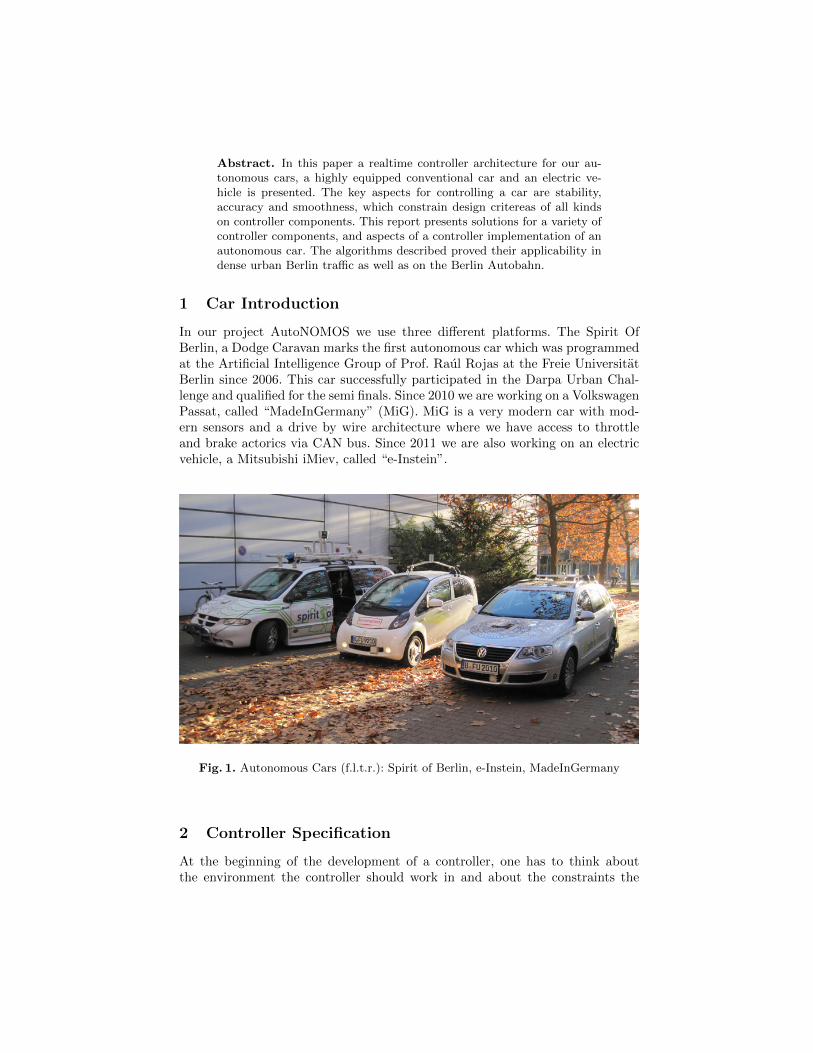
In our project AutoNOMOS we use three different platforms. The Spirit OfBerlin, a Dodge Caravan marks the first autonomous car which was programmedat the Artificial Intelligence Group of Prof. Raul Rojas at the Freie UniversitatBerlin since 2006. This car successfully participated in the Darpa Urban Chal-lenge and qualified for the semi finals. Since 2010 we are working on a VolkswagenPassat, called “MadeInGermany” (MiG). MiG is a very modern car with mod-ern sensors and a drive by wire architecture where we have access to throttleand brake actorics via CAN bus. Since 2011 we are also working on an electricvehicle, a Mitsubishi iMiev, called “e-Instein”.

Fig. 1. Autonomous Cars (f.l.t.r.): Spirit of Berlin, e-Instein, MadeInGermany

2 Controller Specification

At the beginning of the development of a controller, one has to think aboutthe environment the controller should work in and about the constraints the

controller has to satisfy. For our autonomous cars, the following specificationaspects were defined:

– Safety: The controller must be fail safe on a high level with regards to soft-ware or hardware failures. Further, the controller must never perform ma-neuvers, which are not safe with respect to the physical limitations of thecar or the environment. It must never operate beyond the mechanical lim-itations of the actoric. To give an example, a controller which operates ona flat street can to make other assumptions about grip in comparison to acontroller which has to operate in off-road scenarios. Regarding actoric, aquickly responding and precisely adjustable actoric allows more aggressivemaneuvers than the one reacting with huge time delays. As a rule of thumbtranslational and centrifugal forces are limited to 40 percent of physicallypossible values.

– Accuracy: Reaching desired control values quickly is most important for asafe driving of the car. Imprecise or slow controllers usually lead to oscilla-tions within the upper controller level or behavior layer. Oscillations are onereason for an uncomfortable driving experience. For MadeInGermany, thegoal was to have a lateral error to the planned trajectory of less than 10 cmat 100 km/h and a velocity error of less than 0.5 km/h.

– Comfort: Besides limiting the amount of lateral and longitudinal forces to alevel which feels comfortable to a modest driver, another important aspectis to limit acceleration changes, i.e., the function of the acceleration vectorover time must be continuous. Changes within the acceleration vector mustremain small for a comfortable feeling of drive.

Some of these aspects contradict each other, e.g., safety and comfort. A safecontroller might try to apply appropriate maneuvers as fast as possible butthis can be uncomfortable, because humans prefer slow changes of accelerations.Further, comfortable maneuvers, e.g., braking late, can sometimes result in dan-gerous situations. The same holds for accuracy. A controller which tries to betoo precise can result in an uncomfortable feeling of drive.

3 Controller and Planning Modules Overview

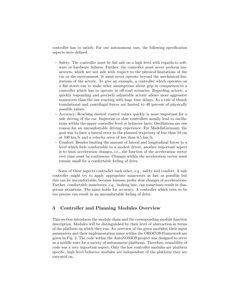
This section introduces the module chain and the corresponding module functiondescription. Modules will be distinguished by their level of abstraction in termsof the platform on which they run. An overview of the given modules, their inputparameters and their implementation name within the OROCOS-Framework aregiven in Fig. 2. The code within the AutoNOMOS project was designed to serveas a middle ware for a variety of autonomous platforms. Therefore, reusability ofcode was a very important aspect. Only the low controller modules are platformspecific, high level behavior modules are independent of the platform they areexecuted on.

a)

b)

c)

Fig. 2. Controller and behavior models. a) For these models, code and data are vehi-cle independent. b) Code is vehicle independent but not data independent. c) Thesemodules are designed for a certain vehicle (VW Passat (MiG)).

4 Steer Control Chain (MiG)

The complete steer control chain includes the module for the behavior, whichgenerates a planned trajectory. The behavior uses a road network definition filewhich includes the streets, and a mission file which defines the checkpoints tobe visited while traveling to a certain destination. Just to mention, the behaviorgenerates in each time frame a new, updated plan, mainly it does not rememberold trajectories. Now, the generated planned trajectory is fed into a lateral con-troller. The task of the lateral controller is to compare the current position of thecar with the alignment of the planned trajectory. Depending on other aspects ascomfort and the current velocity, the lateral controller generates a wanted (de-sired) steering wheel angle. It was assumed there is a linear dependency betweensteering wheel angle and the angle of the front wheel, even though it is knownthat this assumption is just a rough approximation. However, for small anglesthis assumption provides a good estimate and bigger steering angles are exe-cuted at low velocities only, where the exact execution of the generated wantedsteering angle is not as important as it is for high velocities. Future work re-mains to approximate the real function between the steering wheel angle and

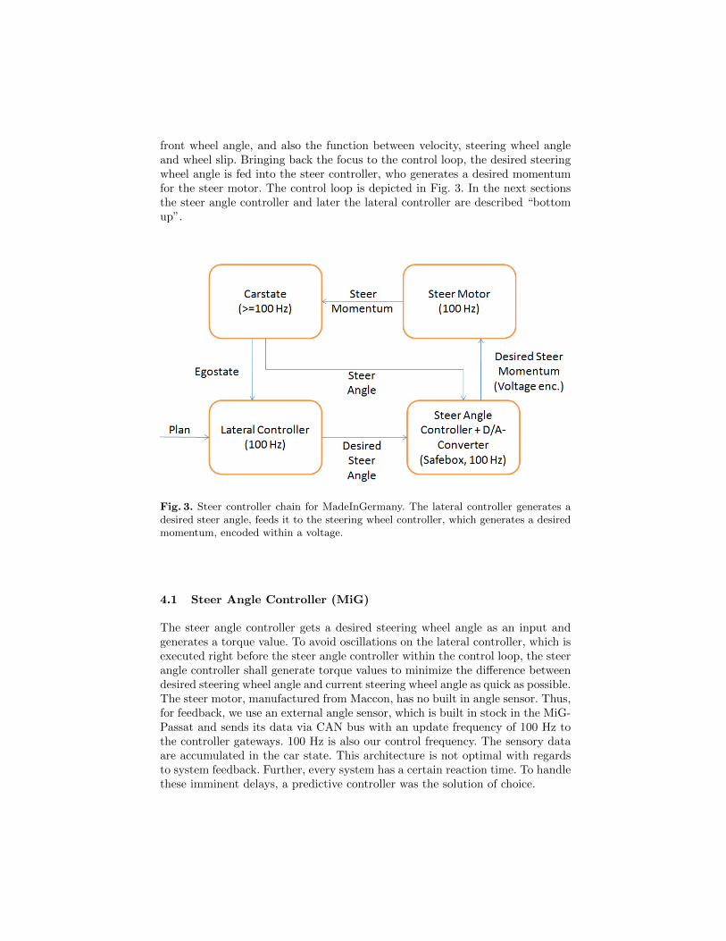
front wheel angle, and also the function between velocity, steering wheel angleand wheel slip. Bringing back the focus to the control loop, the desired steeringwheel angle is fed into the steer controller, who generates a desired momentumfor the steer motor. The control loop is depicted in Fig. 3. In the next sectionsthe steer angle controller and later the lateral controller are described “bottomup”.

Fig. 3. Steer controller chain for MadeInGermany. The lateral controller generates adesired steer angle, feeds it to the steering wheel controller, which generates a desiredmomentum, encoded within a voltage.

4.1 Steer Angle Controller (MiG)

The steer angle controller gets a desired steering wheel angle as an input andgenerates a torque value. To avoid oscillations on the lateral controller, which isexecuted right before the steer angle controller within the control loop, the steerangle controller shall generate torque values to minimize the difference betweendesired steering wheel angle and current steering wheel angle as quick as possible.The steer motor, manufactured from Maccon, has no built in angle sensor. Thus,for feedback, we use an external angle sensor, which is built in stock in the MiG-Passat and sends its data via CAN bus with an update frequency of 100 Hz tothe controller gateways. 100 Hz is also our control frequency. The sensory dataare accumulated in the car state. This architecture is not optimal with regardsto system feedback. Further, every system has a certain reaction time. To handlethese imminent delays, a predictive controller was the solution of choice.

0

05

001

051

002

052

003

002100010080060040020

06-

04-

02-

0

02

04

06

08

Ste

er a

ngle

in d

eg

stee

r mom

entu

m in

per

cent

sm ni emit

tnegnat gninrut

seerged ni elgna reets derusaem

% ni mutnemom reets derised

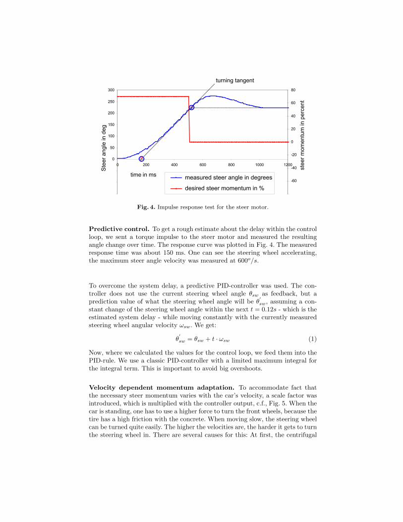
Fig. 4. Impulse response test for the steer motor.

Predictive control. To get a rough estimate about the delay within the controlloop, we sent a torque impulse to the steer motor and measured the resultingangle change over time. The response curve was plotted in Fig. 4. The measuredresponse time was about 150 ms. One can see the steering wheel accelerating,the maximum steer angle velocity was measured at 600o/s.

To overcome the system delay, a predictive PID-controller was used. The con-troller does not use the current steering wheel angle θsw as feedback, but aprediction value of what the steering wheel angle will be θ

′

sw, assuming a con-stant change of the steering wheel angle within the next t = 0.12s - which is theestimated system delay - while moving constantly with the currently measuredsteering wheel angular velocity ωsw. We get:

θ′

sw = θsw + t · ωsw (1)

Now, where we calculated the values for the control loop, we feed them into thePID-rule. We use a classic PID-controller with a limited maximum integral forthe integral term. This is important to avoid big overshoots.

Velocity dependent momentum adaptation. To accommodate fact thatthe necessary steer momentum varies with the car’s velocity, a scale factor wasintroduced, which is multiplied with the controller output, c.f., Fig. 5. When thecar is standing, one has to use a higher force to turn the front wheels, because thetire has a high friction with the concrete. When moving slow, the steering wheelcan be turned quite easily. The higher the velocities are, the harder it gets to turnthe steering wheel in. There are several causes for this: At first, the centrifugal

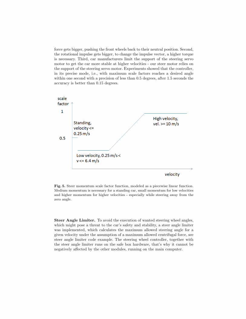
force gets bigger, pushing the front wheels back to their neutral position. Second,the rotational impulse gets bigger, to change the impulse vector, a higher torqueis necessary. Third, car manufacturers limit the support of the steering servomotor to get the car more stable at higher velocities - our steer motor relies onthe support of the steering servo motor. Experiments showed that the controller,in its precise mode, i.e., with maximum scale factors reaches a desired anglewithin one second with a precision of less than 0.5 degrees, after 1.5 seconds theaccuracy is better than 0.15 degrees.

Fig. 5. Steer momentum scale factor function, modeled as a piecewise linear function.Medium momentum is necessary for a standing car, small momentum for low velocitiesand higher momentum for higher velocities - especially while steering away from thezero angle.

Steer Angle Limiter. To avoid the execution of wanted steering wheel angles,which might pose a threat to the car’s safety and stability, a steer angle limiterwas implemented, which calculates the maximum allowed steering angle for agiven velocity under the assumption of a maximum allowed centrifugal force, seesteer angle limiter code example. The steering wheel controller, together withthe steer angle limiter runs on the safe box hardware, that’s why it cannot benegatively affected by the other modules, running on the main computer.

/∗∗∗∗∗∗∗ Steer Angle Limiter ∗∗∗∗∗∗∗/f loat getMaxSteeringWheelAngle ( t o l e r a n c e ) {mSinMaxFWAngle = fabs (WHEELBASE ∗ MAXLATERALACCELERATION /( mAvgFrontWheelSpeeds ∗ mAvgFrontWheelSpeeds ) ) ;i f ( ( mAvgFrontWheelSpeeds != 0 . 0 ) && (mSinMaxFWAngle < 1) ) {

maxWheelAngleAtGivenSpeed = as in (mSinMaxFWAngle) ∗ 180 / Pi ;return f abs ( ( maxWheelAngleAtGivenSpeed /MAXWHEELANGLE ∗ MAXSTEERINGWHEELANGLE) + t o l e r a n c e ) ;

}return MAXSTEERINGWHEELANGLE; // in degrees}

5 Steer Controller Chain (e-Instein)

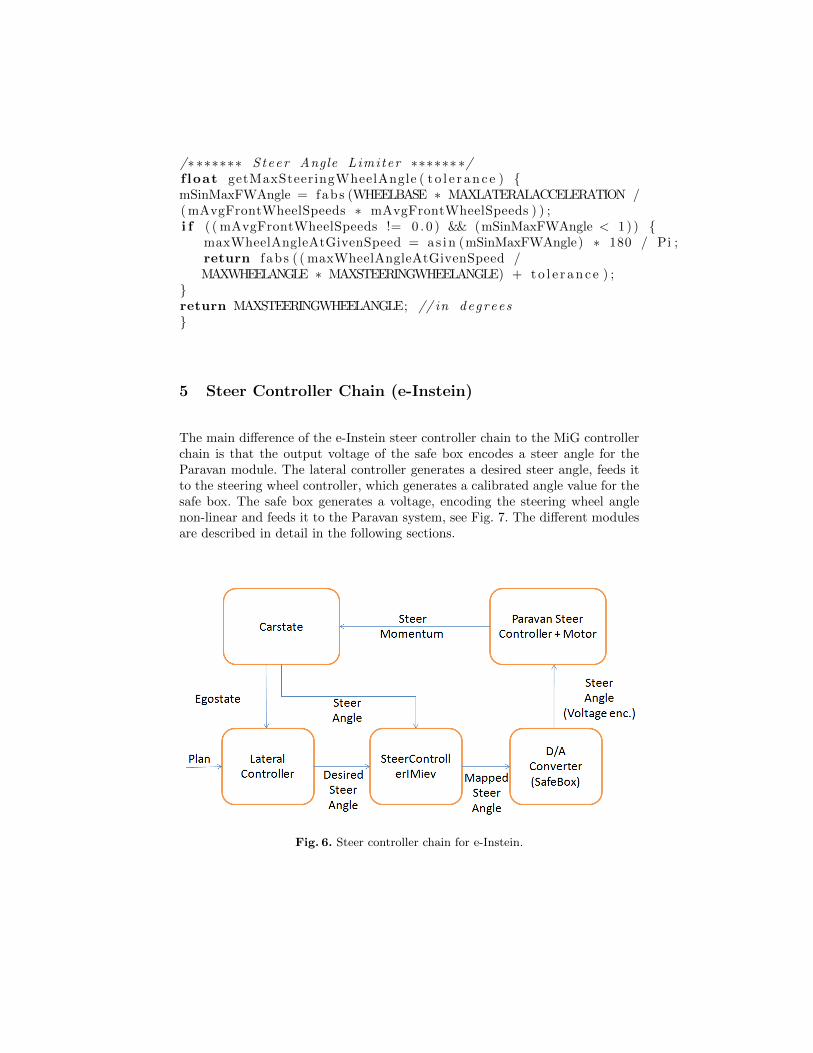
The main difference of the e-Instein steer controller chain to the MiG controllerchain is that the output voltage of the safe box encodes a steer angle for theParavan module. The lateral controller generates a desired steer angle, feeds itto the steering wheel controller, which generates a calibrated angle value for thesafe box. The safe box generates a voltage, encoding the steering wheel anglenon-linear and feeds it to the Paravan system, see Fig. 7. The different modulesare described in detail in the following sections.

Fig. 6. Steer controller chain for e-Instein.

-600

-400

-200

0

200

400

600

-400,00 -200,00 0,00 200,00 400,00input angle in deg

output angle in deg

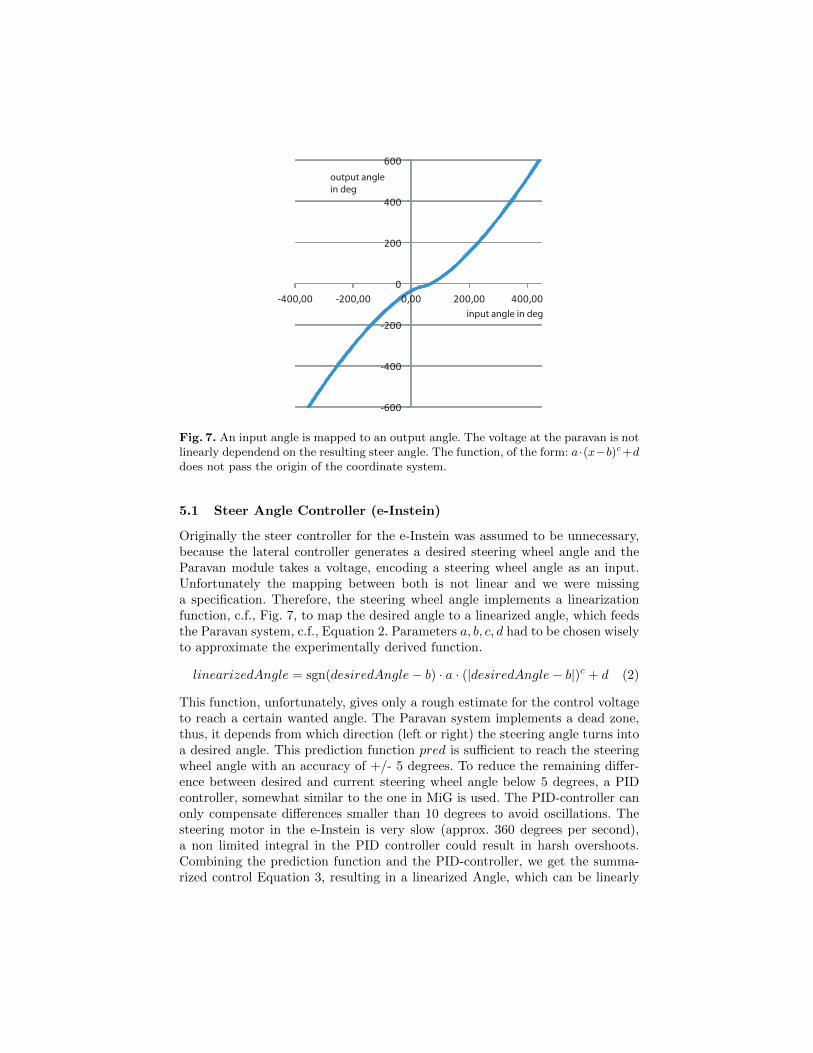
Fig. 7. An input angle is mapped to an output angle. The voltage at the paravan is notlinearly dependend on the resulting steer angle. The function, of the form: a·(x−b)c+ddoes not pass the origin of the coordinate system.

5.1 Steer Angle Controller (e-Instein)

Originally the steer controller for the e-Instein was assumed to be unnecessary,because the lateral controller generates a desired steering wheel angle and theParavan module takes a voltage, encoding a steering wheel angle as an input.Unfortunately the mapping between both is not linear and we were missinga specification. Therefore, the steering wheel angle implements a linearizationfunction, c.f., Fig. 7, to map the desired angle to a linearized angle, which feedsthe Paravan system, c.f., Equation 2. Parameters a, b, c, d had to be chosen wiselyto approximate the experimentally derived function.

linearizedAngle = sgn(desiredAngle− b) · a · (|desiredAngle− b|)c + d (2)

This function, unfortunately, gives only a rough estimate for the control voltageto reach a certain wanted angle. The Paravan system implements a dead zone,thus, it depends from which direction (left or right) the steering angle turns intoa desired angle. This prediction function pred is sufficient to reach the steeringwheel angle with an accuracy of +/- 5 degrees. To reduce the remaining differ-ence between desired and current steering wheel angle below 5 degrees, a PIDcontroller, somewhat similar to the one in MiG is used. The PID-controller canonly compensate differences smaller than 10 degrees to avoid oscillations. Thesteering motor in the e-Instein is very slow (approx. 360 degrees per second),a non limited integral in the PID controller could result in harsh overshoots.Combining the prediction function and the PID-controller, we get the summa-rized control Equation 3, resulting in a linearized Angle, which can be linearly

encoded to a voltage, which again feeds the Paravan box.

linearizedAngle = pred(desiredAngle) + pid(desiredAngle, currentAngle)(3)

The combined control form allow to reach a desired steering wheel angle withan accuracy below 1 degree, within one second - assumed the desired steeringwheel angle is not too far away from the current one.

5.2 Lateral Controller (MiG and e-Instein)

The task of the lateral controller is to generate a desired steer angle to stabilizethe car on the planned trajectory. Thereby the car must not swing left and rightof the trajectory. To fulfill the control task a velocity adaptive PD controller wasimplemented.

vehicle

trajectory

correction angle to return to trajectory

return pointpreview distanceclosest pt.

on traject.

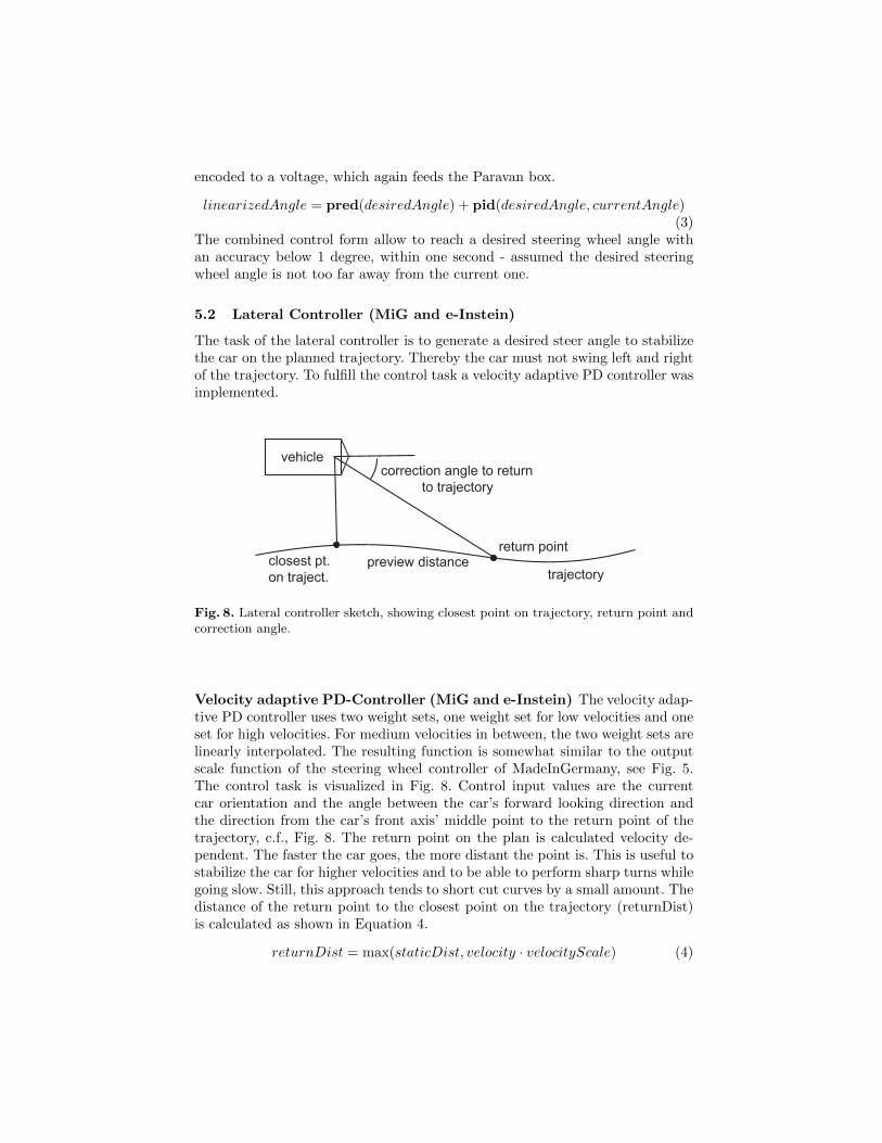
Fig. 8. Lateral controller sketch, showing closest point on trajectory, return point andcorrection angle.

Velocity adaptive PD-Controller (MiG and e-Instein) The velocity adap-tive PD controller uses two weight sets, one weight set for low velocities and oneset for high velocities. For medium velocities in between, the two weight sets arelinearly interpolated. The resulting function is somewhat similar to the outputscale function of the steering wheel controller of MadeInGermany, see Fig. 5.The control task is visualized in Fig. 8. Control input values are the currentcar orientation and the angle between the car’s forward looking direction andthe direction from the car’s front axis’ middle point to the return point of thetrajectory, c.f., Fig. 8. The return point on the plan is calculated velocity de-pendent. The faster the car goes, the more distant the point is. This is useful tostabilize the car for higher velocities and to be able to perform sharp turns whilegoing slow. Still, this approach tends to short cut curves by a small amount. Thedistance of the return point to the closest point on the trajectory (returnDist)is calculated as shown in Equation 4.

returnDist = max(staticDist, velocity · velocityScale) (4)

The static distance value makes sure that the distance to the return point nevergets smaller than a certain value, also when the car is standing. It was set to 2meters in praxis, the scale factor was set to 1 s, which means that the returnpoint is usually reached within one second, if the plan would be kept. In praxis,the car converges to the plan, only, because the desired angle is calculated eachtime again, converging to zero but never reaching zero.

position x

po

siti

on

y

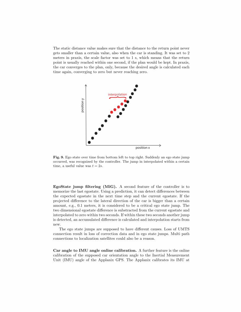
interpolation{Fig. 9. Ego state over time from bottom left to top right. Suddenly an ego state jumpoccurred, was recognized by the controller. The jump in interpolated within a certaintime, a useful value was t = 2s.

EgoState jump filtering (MiG). A second feature of the controller is tomemorize the last egostate. Using a prediction, it can detect differences betweenthe expected egostate in the next time step and the current egostate. If theprojected difference to the lateral direction of the car is bigger than a certainamount, e.g., 0.1 meters, it is considered to be a critical ego state jump. Thetwo dimensional egostate difference is substracted from the current egostate andinterpolated to zero within two seconds. If within these two seconds another jumpis detected, an accumulated difference is calculated and interpolation starts fromnew.

The ego state jumps are supposed to have different causes. Loss of UMTSconnection result in loss of correction data and in ego state jumps. Multi pathconnections to localization satellites could also be a reason.

Car angle to IMU angle online calibration. A further feature is the onlinecalibration of the supposed car orientation angle to the Inertial MeasurementUnit (IMU) angle of the Applanix GPS. The Applanix calibrates its IMU at

every restart. Thus, the difference angle between IMU and car forward directionchanges every time about 0.05 degrees, in worst case scenarios, whenever thecalibration routine was ignored up to 0.5 degrees. At velocities of 100 km/h, 0.5degrees wrongly calibrated IMU can result in a trajectory offset of 0.5 - 1 meter.Therefore a second calibration routine was implemented in the controller. Whengoing almost straight and going faster than 60 km/h, the controller integratesthe error to the trajectory over a certain time span, a useful value was t = 4s. Ifthe integral was significantly below or beyond zero, an small positive or negativeoffset value is added to the car orientation angle. Thus, after ten iterations, i.e.,within a minute, the IMU offset could be successfully neutralized.

Engaged,Gear Neutral

velocity < 3 m/s

Brake

velocity = 0 m/s

Shift into R, D or S

velocity >= 3 m/s

driver intervention

driver intervention

Disengaged

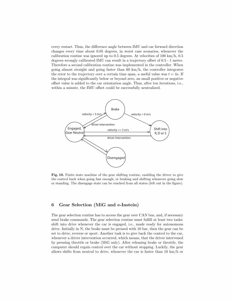
Fig. 10. Finite state machine of the gear shifting routine, enabling the driver to givethe control back when going fast enough, or braking and shifting whenever going slowor standing. The disengage state can be reached from all states (left out in the figure).

6 Gear Selection (MiG and e-Instein)

The gear selection routine has to access the gear over CAN bus, and, if necessarysend brake commands. The gear selection routine must fulfill at least two tasks:shift into drive whenever the car is engaged, i.e., made ready for autonomousdrive. Initially in N, the brake must be pressed with 10 bar, then the gear can beset to drive, reverse or sport. Another task is to give back the control to the car,whenever a driver intervention occurred, which means, that the driver intervenedby pressing throttle or brake (MiG only). After releasing brake or throttle, thecomputer should regain control over the car without stopping. Luckily, the gearallows shifts from neutral to drive, whenever the car is faster than 10 km/h or

approx. 3 meters per second. The finite state machine, depicted in Fig. 10 givesan idea about the functionality of the gear setting routine.

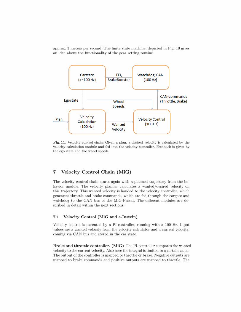
Fig. 11. Velocity control chain: Given a plan, a desired velocity is calculated by thevelocity calculation module and fed into the velocity controller. Feedback is given bythe ego state and the wheel speeds.

7 Velocity Control Chain (MiG)

The velocity control chain starts again with a planned trajectory from the be-havior module. The velocity planner calculates a wanted/desired velocity onthis trajectory. This wanted velocity is handed to the velocity controller, whichgenerates throttle and brake commands, which are fed through the cargate andwatchdog to the CAN bus of the MiG-Passat. The different modules are de-scribed in detail within the next sections.

7.1 Velocity Control (MiG and e-Instein)

Velocity control is executed by a PI-controller, running with a 100 Hz. Inputvalues are a wanted velocity from the velocity calculator and a current velocity,coming via CAN bus and stored in the car state.

Brake and throttle controller. (MiG) The PI-controller compares the wantedvelocity to the current velocity. Also here the integral is limited to a certain value.The output of the controller is mapped to throttle or brake. Negative outputs aremapped to brake commands and positive outputs are mapped to throttle. The

most important aspect here lies in the fact, that throttle and brake commandshave different effects, i.e., 50 percent of brake results in much higher accelera-tion amounts than 50 percent of throttle. That is why positive outputs of thecontroller were weighted with a throttleConstant, which was set to 4.

Throttle and brake limitations. (MiG) For a comfortable ride, the brakecommands were limited to 32 percent of their maximum value, which can result inup to 6ms−2 deceleration. This was especially important for testing the obstacletracker. To give an example, wrongly classified obstacles could have a devastatingeffect when going with a 100 km/h on the highway, if they resulted in a fullbrake, endangering especially the following cars. Also the throttle commandswere limited to 50 percent of their maximum during normal velocities. Whenstarting to move, this value was limited to 35 percent and linearly interpolatedto 50 percent at a velocity of 5 meters per second.

For a racetrack scenario, much higher thresholds were applied and can beactivated through a flag. In this case, the steering angle limiter from Section 4.1must be deactivated on the safe box as well.

Dynamic Handbrake. (MiG and e-Instein) Stopping a car needs specialtreatment. A car with an automatic gear tends to start rolling, even withoutany throttle or brake commands. The integral part of the PI-controller musthave an integral weight together with a maximum integral value, big enough tostop the car. This alone is no difference to any other velocity to control. Butif the desired velocity is set to zero, the controller tends to convergence to thewanted velocity or it swings around the wanted velocity, resulting in a stop andgo. Thus, without special treatment, it can take several seconds to reach a fullstop with the car. Further, if pressing the brake not hard enough, the Passat car(MiG) will not fully open the clutch of its direct shift gear, resulting in a semiclosed clutch, which again causes severe damage to the clutch over time. A nicesolution is to add an increasing amount of brake pressure over time, wheneverthe wanted velocity is set to zero, combined with the fact that the car is alreadyslower than 4 meters per second. If the car is actually standing, a further fixedamount of brake pressure is added to the brake, to make sure, the clutch isfully open. This “dynamic handbrake” is also useful when stopping at a steepmountain to make sure the car will stop. In experiments the controller provedto be able to keep all velocities up to 100 km/h with an accuracy of 0.5 km/h.

7.2 Velocity Calculation (MiG and e-Instein)

The velocity calculation module is independent of the car it is running on. Im-portant parameters for the velocity calculation are maximum allowed centrifugalaccelerations and brake accelerations. These values are referred to as “comfortsettings”. The velocity calculation is generated instantly and recalculated eachtime step again. There are different aspects which have an effect on the currentlydesired velocity: static obstacles or traffic signs/lights on the planned trajectory,

dynamic obstacles on the trajectory, curves in front with a certain curvature andat a certain distance, , and of course the officially allowed velocity. All aspectson the trajectory result in a maximum velocity at which they can be approachedcurrently, e.g., a curve in a distance of 5 meters results in a lower currently de-sired velocity than the same curve in 50 meters distance. For reasons of safety,from all desired velocities the smallest one is returned to the velocity controller.

The following sections will give a glimpse about the different calculations,which all use the same core function.

Velocity calculation for static obstacles. A first assumption when brakingtowards a static obstacle was, that the braking acceleration a shall be constantover the whole time. Let us assume, a static obstacle was detected in a certaindistance ∆s. To brake down with a constant acceleration a (brake accelerationsare negative) and to stop right in front of the obstacle, the current desiredvelocity vd is calculated as follows:

vd =√−2a∆s (5)

vd = (−2a · (obstaclePosition− carPosition))0.5 (6)

vd = (−2a · (obstaclePosition− carPosition))b (7)

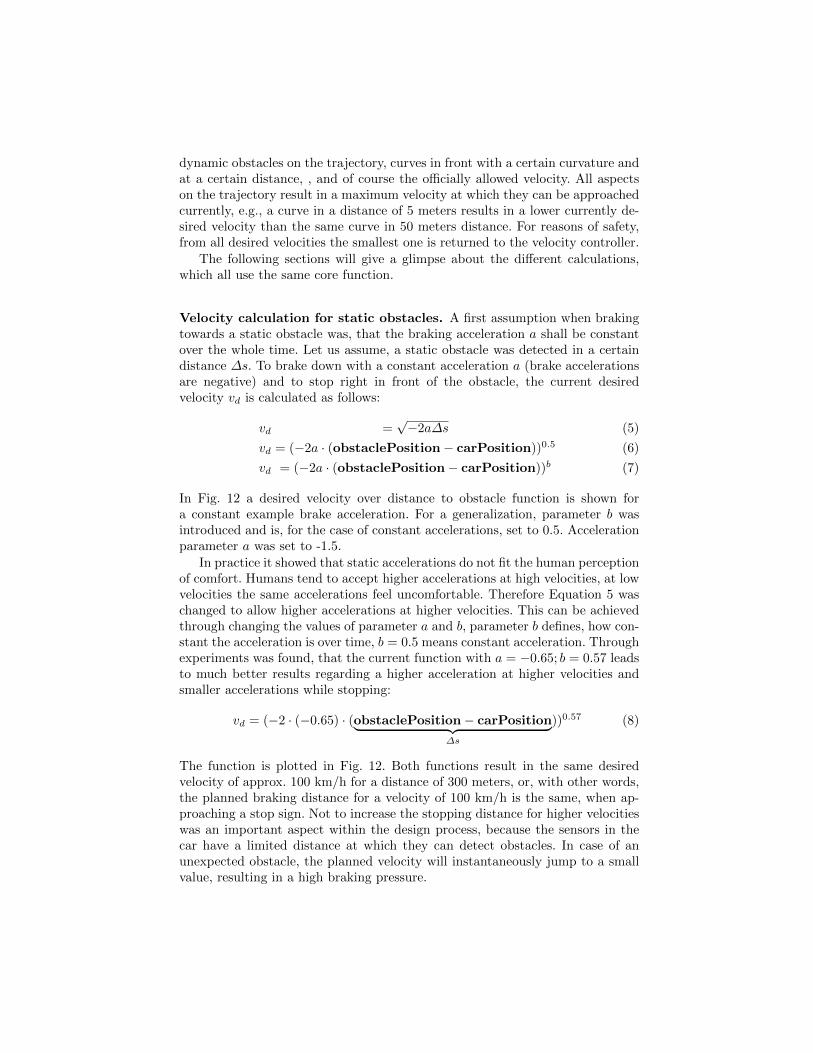
In Fig. 12 a desired velocity over distance to obstacle function is shown fora constant example brake acceleration. For a generalization, parameter b wasintroduced and is, for the case of constant accelerations, set to 0.5. Accelerationparameter a was set to -1.5.

In practice it showed that static accelerations do not fit the human perceptionof comfort. Humans tend to accept higher accelerations at high velocities, at lowvelocities the same accelerations feel uncomfortable. Therefore Equation 5 waschanged to allow higher accelerations at higher velocities. This can be achievedthrough changing the values of parameter a and b, parameter b defines, how con-stant the acceleration is over time, b = 0.5 means constant acceleration. Throughexperiments was found, that the current function with a = −0.65; b = 0.57 leadsto much better results regarding a higher acceleration at higher velocities andsmaller accelerations while stopping:

vd = (−2 · (−0.65) · (obstaclePosition− carPosition︸︷︷︸∆s

))0.57 (8)

The function is plotted in Fig. 12. Both functions result in the same desiredvelocity of approx. 100 km/h for a distance of 300 meters, or, with other words,the planned braking distance for a velocity of 100 km/h is the same, when ap-proaching a stop sign. Not to increase the stopping distance for higher velocitieswas an important aspect within the design process, because the sensors in thecar have a limited distance at which they can detect obstacles. In case of anunexpected obstacle, the planned velocity will instantaneously jump to a smallvalue, resulting in a high braking pressure.

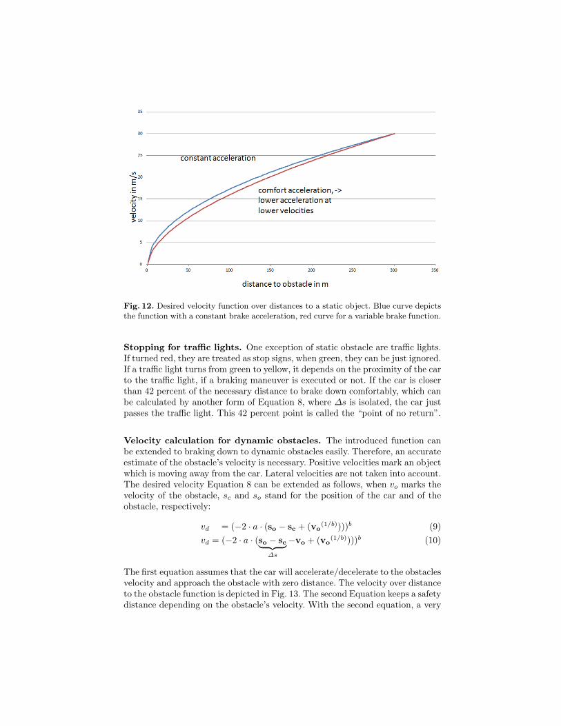
Fig. 12. Desired velocity function over distances to a static object. Blue curve depictsthe function with a constant brake acceleration, red curve for a variable brake function.

Stopping for traffic lights. One exception of static obstacle are traffic lights.If turned red, they are treated as stop signs, when green, they can be just ignored.If a traffic light turns from green to yellow, it depends on the proximity of the carto the traffic light, if a braking maneuver is executed or not. If the car is closerthan 42 percent of the necessary distance to brake down comfortably, which canbe calculated by another form of Equation 8, where ∆s is isolated, the car justpasses the traffic light. This 42 percent point is called the “point of no return”.

Velocity calculation for dynamic obstacles. The introduced function canbe extended to braking down to dynamic obstacles easily. Therefore, an accurateestimate of the obstacle’s velocity is necessary. Positive velocities mark an objectwhich is moving away from the car. Lateral velocities are not taken into account.The desired velocity Equation 8 can be extended as follows, when vo marks thevelocity of the obstacle, sc and so stand for the position of the car and of theobstacle, respectively:

vd = (−2 · a · (so − sc + (vo(1/b))))b (9)

vd = (−2 · a · (so − sc︸︷︷︸∆s

−vo + (vo(1/b))))b (10)

The first equation assumes that the car will accelerate/decelerate to the obstaclesvelocity and approach the obstacle with zero distance. The velocity over distanceto the obstacle function is depicted in Fig. 13. The second Equation keeps a safetydistance depending on the obstacle’s velocity. With the second equation, a very

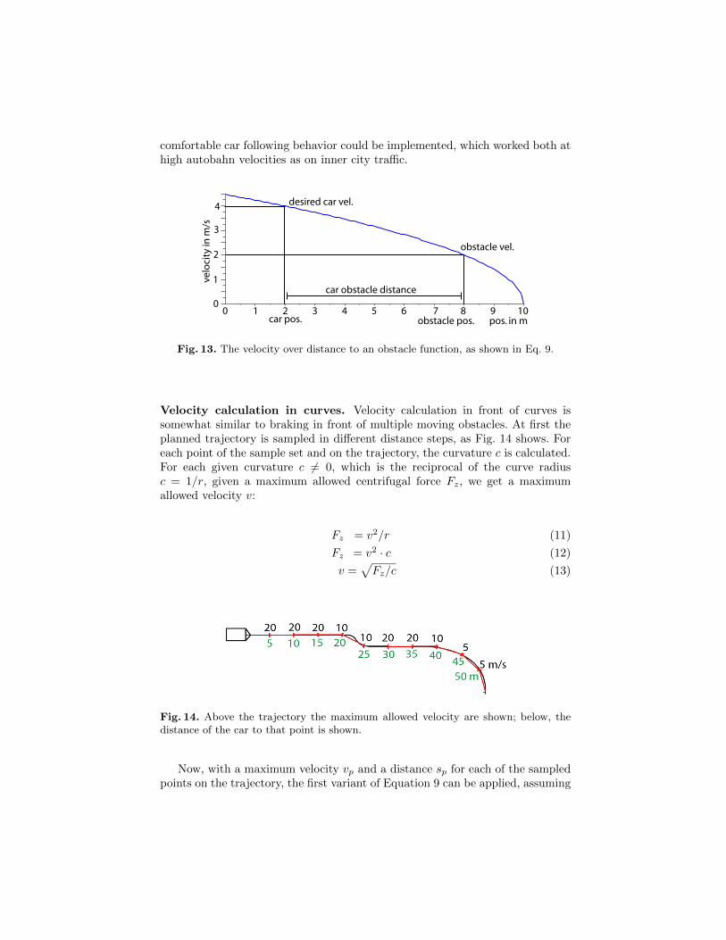
comfortable car following behavior could be implemented, which worked both athigh autobahn velocities as on inner city traffic.

0 1 2 3 4 5 6 7 8 9 10pos. in m

obstacle vel.

0

1

2

3

4ve

loci

ty in

m/s

car obstacle distance

desired car vel.

car pos. obstacle pos.

Fig. 13. The velocity over distance to an obstacle function, as shown in Eq. 9.

Velocity calculation in curves. Velocity calculation in front of curves issomewhat similar to braking in front of multiple moving obstacles. At first theplanned trajectory is sampled in different distance steps, as Fig. 14 shows. Foreach point of the sample set and on the trajectory, the curvature c is calculated.For each given curvature c 6= 0, which is the reciprocal of the curve radiusc = 1/r, given a maximum allowed centrifugal force Fz, we get a maximumallowed velocity v:

Fz = v2/r (11)

Fz = v2 · c (12)

v =√Fz/c (13)

Fig. 14. Above the trajectory the maximum allowed velocity are shown; below, thedistance of the car to that point is shown.

Now, with a maximum velocity vp and a distance sp for each of the sampledpoints on the trajectory, the first variant of Equation 9 can be applied, assuming

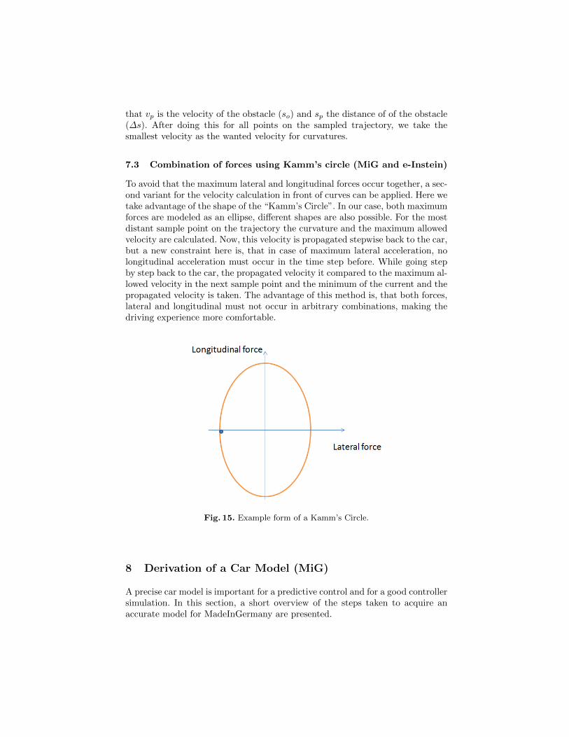
that vp is the velocity of the obstacle (so) and sp the distance of of the obstacle(∆s). After doing this for all points on the sampled trajectory, we take thesmallest velocity as the wanted velocity for curvatures.

7.3 Combination of forces using Kamm’s circle (MiG and e-Instein)

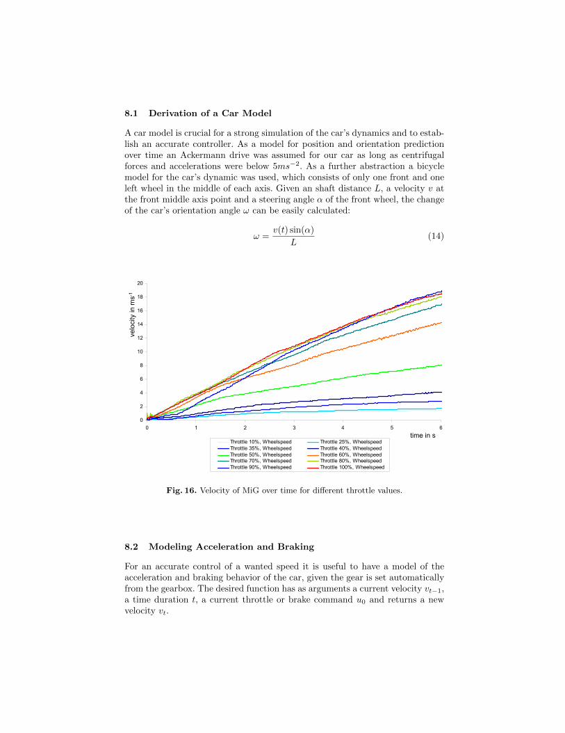
To avoid that the maximum lateral and longitudinal forces occur together, a sec-ond variant for the velocity calculation in front of curves can be applied. Here wetake advantage of the shape of the “Kamm’s Circle”. In our case, both maximumforces are modeled as an ellipse, different shapes are also possible. For the mostdistant sample point on the trajectory the curvature and the maximum allowedvelocity are calculated. Now, this velocity is propagated stepwise back to the car,but a new constraint here is, that in case of maximum lateral acceleration, nolongitudinal acceleration must occur in the time step before. While going stepby step back to the car, the propagated velocity it compared to the maximum al-lowed velocity in the next sample point and the minimum of the current and thepropagated velocity is taken. The advantage of this method is, that both forces,lateral and longitudinal must not occur in arbitrary combinations, making thedriving experience more comfortable.

Fig. 15. Example form of a Kamm’s Circle.

8 Derivation of a Car Model (MiG)

A precise car model is important for a predictive control and for a good controllersimulation. In this section, a short overview of the steps taken to acquire anaccurate model for MadeInGermany are presented.

8.1 Derivation of a Car Model

A car model is crucial for a strong simulation of the car’s dynamics and to estab-lish an accurate controller. As a model for position and orientation predictionover time an Ackermann drive was assumed for our car as long as centrifugalforces and accelerations were below 5ms−2. As a further abstraction a bicyclemodel for the car’s dynamic was used, which consists of only one front and oneleft wheel in the middle of each axis. Given an shaft distance L, a velocity v atthe front middle axis point and a steering angle α of the front wheel, the changeof the car’s orientation angle ω can be easily calculated:

ω =v(t) sin(α)

L(14)

Daniel Göhring16. August 2010

Bestimmung Aktuatorparameter MiG: Motor, Bremse, Lenkung

Institut für InformatikAG Künstliche Intelligenz

4

Geschwindigkeits-Zeitkurve (Motor)

0

2

4

6

8

10

12

14

16

18

20

0 1 2 3 4 5 6

Throttle 10%, Wheelspeed Throttle 25%, WheelspeedThrottle 35%, Wheelspeed Throttle 40%, WheelspeedThrottle 50%, Wheelspeed Throttle 60%, WheelspeedThrottle 70%, Wheelspeed Throttle 80%, WheelspeedThrottle 90%, Wheelspeed Throttle 100%, Wheelspeed

velo

city

in m

s-1

time in s

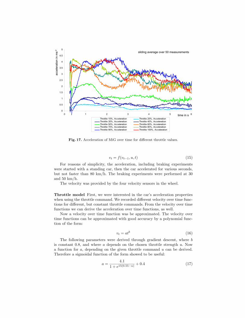
Fig. 16. Velocity of MiG over time for different throttle values.

8.2 Modeling Acceleration and Braking

For an accurate control of a wanted speed it is useful to have a model of theacceleration and braking behavior of the car, given the gear is set automaticallyfrom the gearbox. The desired function has as arguments a current velocity vt−1,a time duration t, a current throttle or brake command u0 and returns a newvelocity vt.




5

0

0.5

1

1.5

2

2.5

3

3.5

4

4.5

5

0 1 2 3 4 5 6

Throttle 10%, Acceleration Throttle 25%, AccelerationThrottle 35%, Acceleration Throttle 40%, AccelerationThrottle 50%, Acceleration Throttle 60%, AccelerationThrottle 70%, Acceleration Throttle 80%, AccelerationThrottle 90%, Acceleration Throttle 100%, Acceleration

Beschleunigungs-Zeitkurve (Motor)

sliding average over 50 measurements

time in s

acce

lera

tion

in m

s-2

Fig. 17. Acceleration of MiG over time for different throttle values.

vt = f(vt−1, u, t) (15)

For reasons of simplicity, the acceleration, including braking experimentswere started with a standing car, then the car accelerated for various seconds,but not faster than 80 km/h. The braking experiments were performed at 30and 50 km/h.

The velocity was provided by the four velocity sensors in the wheel.

Throttle model First, we were interested in the car’s acceleration propertieswhen using the throttle command. We recorded different velocity over time func-tions for different, but constant throttle commands. From the velocity over timefunctions we can derive the acceleration over time functions, as well.

Now a velocity over time function was be approximated. The velocity overtime functions can be approximated with good accuracy by a polynomial func-tion of the form:

vt = atb (16)

The following parameters were derived through gradient descent, where bis constant 0.8, and where a depends on the chosen throttle strength u. Nowa function for a, depending on the given throttle command u can be derived.Therefore a sigmoidal function of the form showed to be useful:

a =4.1

1 + e15(0.55−u)+ 0.4 (17)

0 1.0

2

0.9

4

0.8

6

0.7 0.6

8

v in

m/s

0.5

relative throttle

10

0.46

12

5 0.34

14

0.23

16

2

time in s 0.1

1

18

0.0 0

20

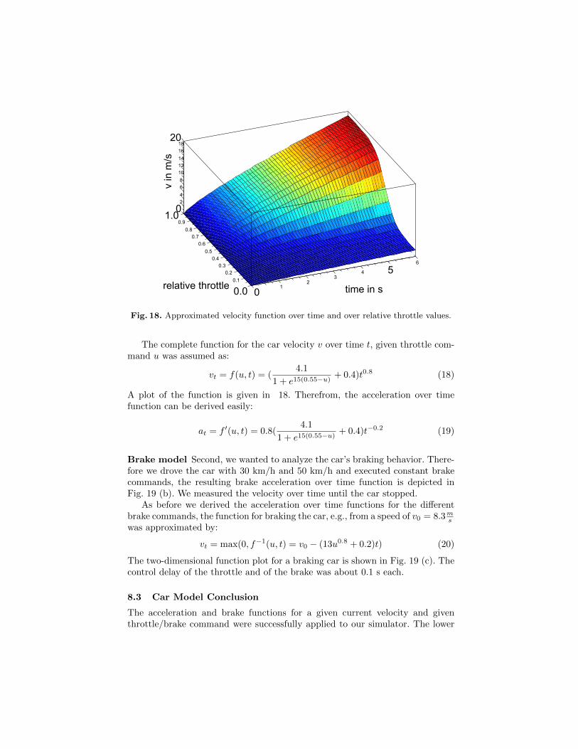
Fig. 18. Approximated velocity function over time and over relative throttle values.

The complete function for the car velocity v over time t, given throttle com-mand u was assumed as:

vt = f(u, t) = (4.1

1 + e15(0.55−u)+ 0.4)t0.8 (18)

A plot of the function is given in 18. Therefrom, the acceleration over timefunction can be derived easily:

at = f ′(u, t) = 0.8(4.1

1 + e15(0.55−u)+ 0.4)t−0.2 (19)

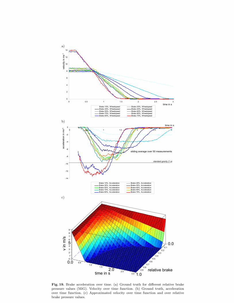
Brake model Second, we wanted to analyze the car’s braking behavior. There-fore we drove the car with 30 km/h and 50 km/h and executed constant brakecommands, the resulting brake acceleration over time function is depicted inFig. 19 (b). We measured the velocity over time until the car stopped.

As before we derived the acceleration over time functions for the differentbrake commands, the function for braking the car, e.g., from a speed of v0 = 8.3mswas approximated by:

vt = max(0, f−1(u, t) = v0 − (13u0.8 + 0.2)t) (20)

The two-dimensional function plot for a braking car is shown in Fig. 19 (c). Thecontrol delay of the throttle and of the brake was about 0.1 s each.

8.3 Car Model Conclusion

The acceleration and brake functions for a given current velocity and giventhrottle/brake command were successfully applied to our simulator. The lower

level controllers still had to be tuned in the real car because of the complexcar dynamics, especially tire slip, mass distribution, system delays and slippagewithin all kinds of gears. However, this simple car model helped significantly todesign the behavior and the higher level controllers within the simulator.

9 Summary

This technical report focussed on the main components of the autonomous cars“MadeInGermany” and “e-Instein”. The specification described at the beginningwas successfully met. MiG was able to safely drive through inner city traffic anddrove also on the Berlin Autobahn with up to 100 km/h, where its mean lateralerror to the trajectory was less than 10 cm. The velocity error was about 0.5km/h. For e-Instein these values are still higher, but work is in progress. Futurework will focus on energy efficient control routines to increase energy efficientcontrol.

a)




6

Geschwindigkeits-Zeitkurve (Bremse)

0

2

4

6

8

10

12

14

0 0.5 1 1.5 2 2.5 3

Brake 10%, Wheelspeed Brake 20%, WheelspeedBrake 30%, Wheelspeed Brake 40%, WheelspeedBrake 50%, Wheelspeed Brake 60%, WheelspeedBrake 70%, Wheelspeed Brake 80%, WheelspeedBrake 60%, Wheelspeed Brake 70%, Wheelspeed

velo

city

in m

s-1

time in s

b)




7

Beschleunigungs-Zeitkurve (Bremse)

-14

-12

-10

-8

-6

-4

-2

00 0.5 1 1.5 2 2.5 3

Brake 10%, Acceleration Brake 20%, AccelerationBrake 30%, Acceleration Brake 40%, AccelerationBrake 50%, Acceleration Brake 60%, AccelerationBrake 70%, Acceleration Brake 80%, AccelerationBrake 60%, Acceleration Brake 70%, Acceleration

standard gravity (1 g)

sliding average over 50 measurements

acce

lera

tion

in m

s-2

time in s

c)

0.00.1

0.20.3

0.40.50

relative brake

0.0 0.60.5

1

0.71.0

2

1.5 0.82.0

time in s0.9

3

2.5

1.03.0

4

v in

m/s

56789

Fig. 19. Brake acceleration over time. (a) Ground truth for different relative brakepressure values (MiG). Velocity over time function. (b) Ground truth, accelerationover time function. (c) Approximated velocity over time function and over relativebrake pressure values.

controller architecture for the autonomous cars...

Documents