control sys demo 10 11
TRANSCRIPT

Good Evening
CONTROL SYSTEM TUTORIAL
with MATALAB
BY
RAVI KUMAR JATOTH
LECTURER
DEPT OF ECE
NIT, WARANGAL
16/03/2011 2Ravi Kumar Jatoth

INTRODUCTION
Computer software can be used to
aid computation and modeling of
system. A program that is often
used is
MATLAB

MATLAB MATLAB stands for MATrix LABoratory
MATLAB is a software package for high performance numerical computation and visualization.
There are many different toolboxes available which extend the basic functions of Matlab into different application areas.
we will make extensive use of the Control Systems Toolbox
16/03/2011 4Ravi Kumar Jatoth

Do Mech guys really need a computer for purposes other than CAD & CAM ? Can you recall these equation –
1∕√f = -2log(2.51/Re√f + 7/3.7d)
How about this one--
Q=(b*yn /n) {b*yn/(b+2yn)}2/3
They had cost many of us as much as 15 to 20
marks last sem in Fluid Mechanics course.
There are several equations for which only numerical
solutions exist.
16/03/2011 5Ravi Kumar Jatoth

MATLAB
Typical uses: Math and computation
Algorithm development
Data acquisition
Modeling, simulation, and prototyping
Data analysis, exploration, and visualization
Scientific and engineering graphics
Application development, including GUI building
16/03/2011 6Ravi Kumar Jatoth
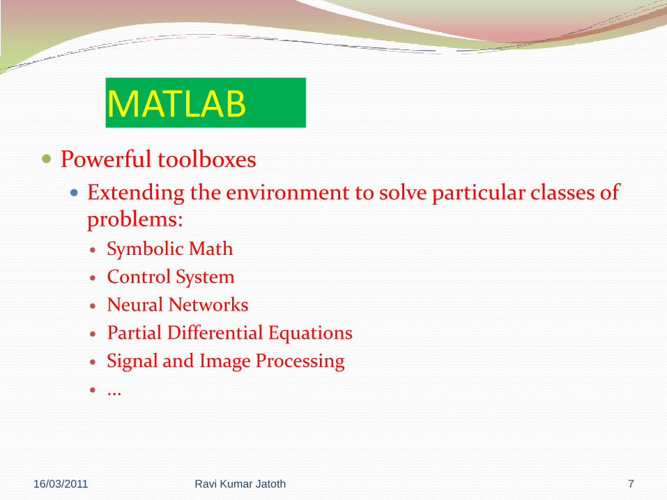
MATLAB Powerful toolboxes
Extending the environment to solve particular classes of problems:
Symbolic Math
Control System
Neural Networks
Partial Differential Equations
Signal and Image Processing
...
16/03/2011 7Ravi Kumar Jatoth

Basics of MATLAB
MATLAB WINDOWS
MATLAB DESKTOP
1.Command window
2.current directory
3.workspace
4.command history
Figure window
Editor window 16/03/2011 8Ravi Kumar Jatoth

MATLAB Desktop
Command
Window
Launch Pad
History
16/03/2011 9Ravi Kumar Jatoth

MATLAB Desktop – cont’d
Command
Window
Workspace
Current
DIrectory
16/03/2011 10Ravi Kumar Jatoth
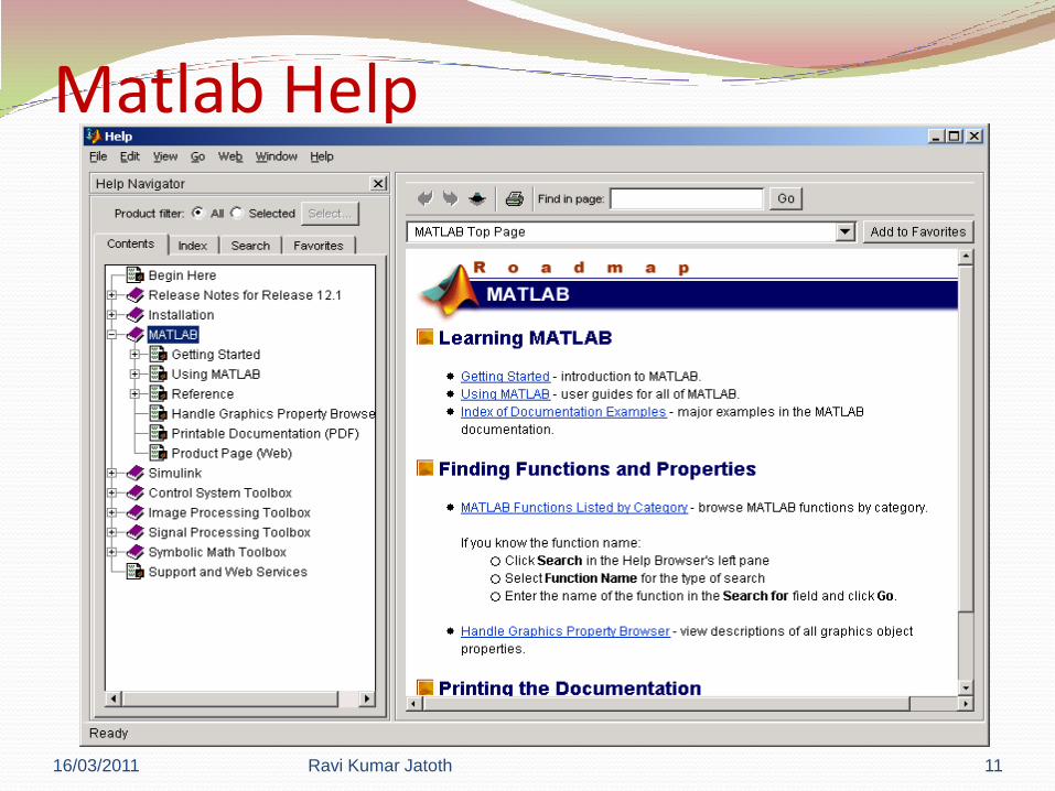
Matlab Help
16/03/2011 11Ravi Kumar Jatoth

Matlab Editor
Color keyed
text with auto
indents
tabbed sheets for other
files being edited
Access to
commands
16/03/2011 12Ravi Kumar Jatoth
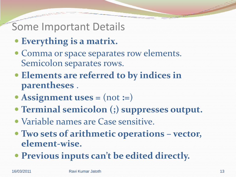
Some Important Details Everything is a matrix.
Comma or space separates row elements.Semicolon separates rows.
Elements are referred to by indices in parentheses .
Assignment uses = (not :=)
Terminal semicolon (;) suppresses output.
Variable names are Case sensitive.
Two sets of arithmetic operations – vector, element-wise.
Previous inputs can’t be edited directly.
16/03/2011 13Ravi Kumar Jatoth
How to Use MATLAB? Command driven:
MATLAB processes single-line commands immediately and displays the result.
Script driven:
MATLAB is also capable of executing sequences of command that are stored in files.
These source files are called m-files, having a .m extension.
16/03/2011 14Ravi Kumar Jatoth

Matlab ProgramsMatlab is an extravagant calculator if all we can do is
execute commands typed into the Command Window… So how can we execute a “program?” Programs in Matlab are: Scripts, or Functions
Scripts: Matlab statements that are fed from a file into the Command Window and executed immediately
Functions: Program modules that are passed data (arguments) and return a result (i.e., sin(x))
These can be created in any text editor (but Matlab supplies a nice built-in editor)
16/03/2011 15Ravi Kumar Jatoth

Reserved Words…
Matlab has some special (reserved) words that you might use while writing programs
for
end
if
while
function
return
elsif
case
otherwise
switch
continue
else
try
catch
global
persistent
break
16/03/2011 16Ravi Kumar Jatoth
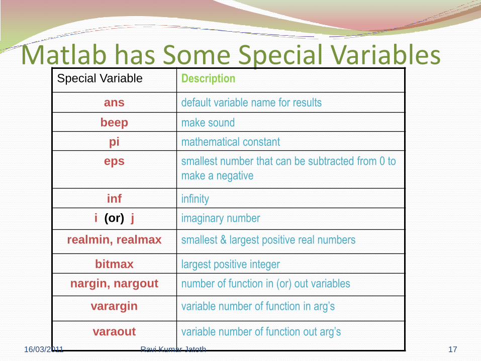
Matlab has Some Special VariablesSpecial Variable Description
ans default variable name for results
beep make sound
pi mathematical constant
eps smallest number that can be subtracted from 0 to
make a negative
inf infinity
i (or) j imaginary number
realmin, realmax smallest & largest positive real numbers
bitmax largest positive integer
nargin, nargout number of function in (or) out variables
varargin variable number of function in arg’s
varaout variable number of function out arg’s
16/03/2011 17Ravi Kumar Jatoth
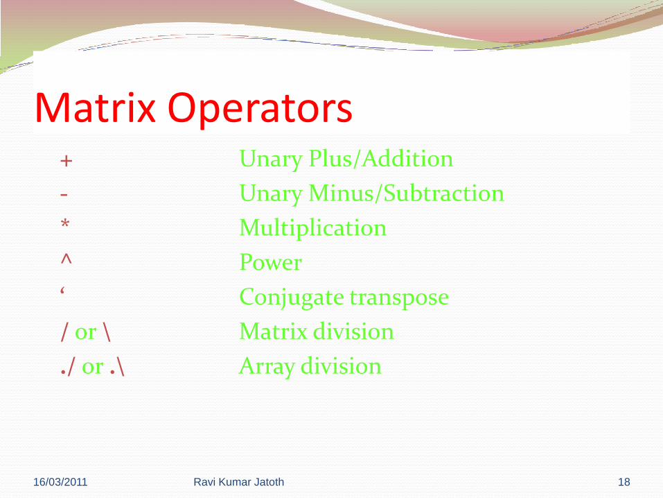
Matrix Operators+ Unary Plus/Addition
- Unary Minus/Subtraction
* Multiplication
^ Power
‘ Conjugate transpose
/ or \ Matrix division
./ or .\ Array division
16/03/2011 18Ravi Kumar Jatoth

Matrix Operators
16/03/2011 19Ravi Kumar Jatoth
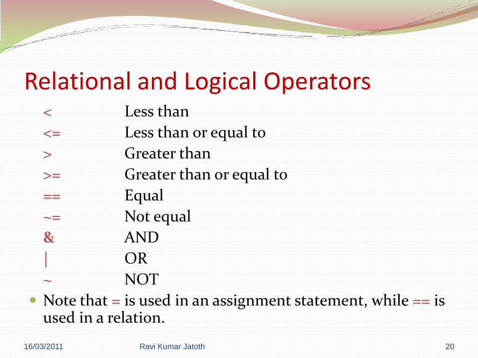
Relational and Logical Operators< Less than
<= Less than or equal to
> Greater than
>= Greater than or equal to
== Equal
~= Not equal
& AND
| OR
~ NOT
Note that = is used in an assignment statement, while == is used in a relation.
16/03/2011 20Ravi Kumar Jatoth
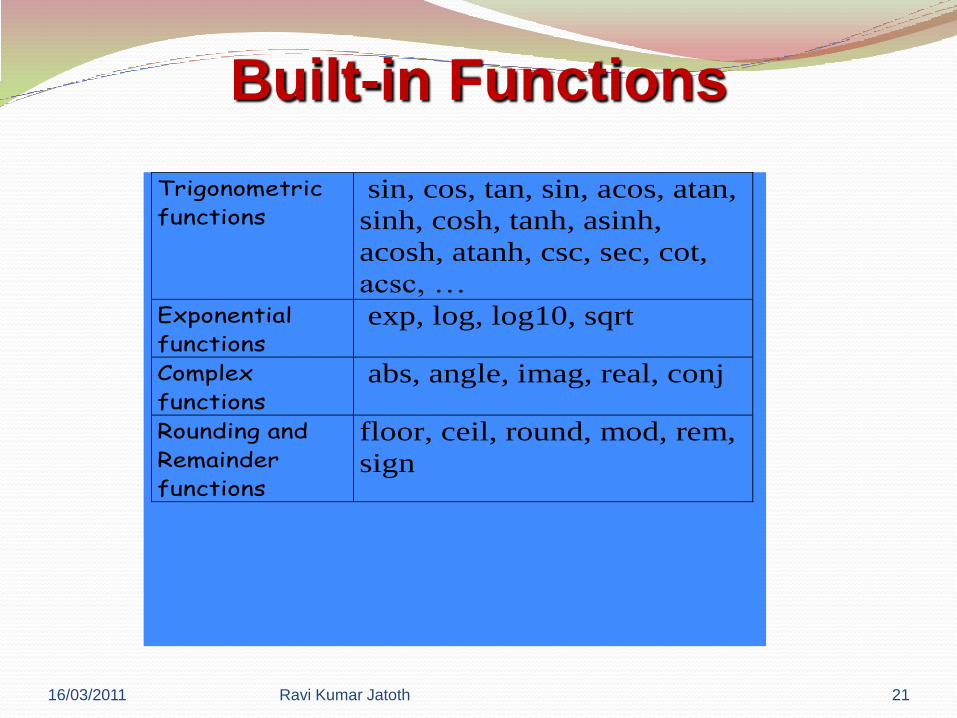
Built-in Functions
Trigonometric
functions sin, cos, tan, sin, acos, atan,
sinh, cosh, tanh, asinh,
acosh, atanh, csc, sec, cot,
acsc, … Exponential
functions exp, log, log10, sqrt
Complex
functions abs, angle, imag, real, conj
Rounding and
Remainder
functions
floor, ceil, round, mod, rem,
sign
16/03/2011 21Ravi Kumar Jatoth

Entering a matrix and assigning it to a variable name
Remember that row elements are separated by comma or space and rows by semicolon or enter
16/03/2011 22Ravi Kumar Jatoth

Matlab Basics Tutorial
Vectors
a = [1 2 3 4 5 6 9 8 7] Let's say you want to create a vector with elements between 0 and 20 evenly spaced in increments
of 2 (this method is frequently used to create a time vector):
t = 0:2:20
Functions
sin(pi/4)
Plotting
X=[0 1 2 3 4 5];
Y=[0 1 4 9 16 25];
plot(X,Y)
16/03/2011 23Ravi Kumar Jatoth

Cont..
Sine wave
t=0:0.25:7;
y = sin(t);
plot(t,y)
X=(0 1 2 3 4 5 6 7);
Y=exp(X);
16/03/2011 24Ravi Kumar Jatoth

Practice Entering Some Expressions
>>4+3*sqrt(2)
>>sin(pi/6)
>>i^2
>>j^2 (For electrical engineers)
>>x=log(10)
>>y=exp(x)
16/03/2011 25Ravi Kumar Jatoth

Matrices
Entering matrices into Matlab is the same as entering a vector, except each
row of elements is separated by a semicolon (;) or a return:
B = [1 2 3 4;5 6 7 8;9 10 11 12]
B = [ 1 2 3 4
5 6 7 8
9 10 11 12]
Matrices in Matlab can be manipulated in many ways. For one, you can find the transpose of a matrix using the apostrophe key:
C = B'
C = 1 5 9
2 6 10
3 7 11
4 8 12
D = B * C
16/03/2011 26Ravi Kumar Jatoth
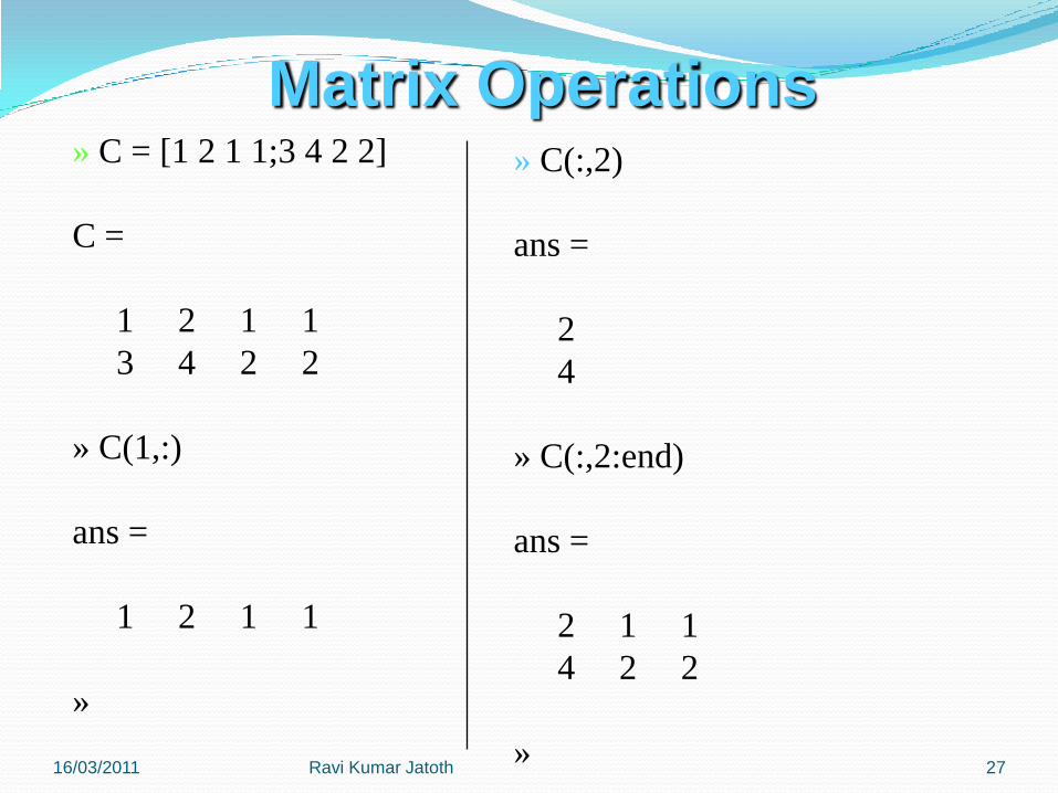
Matrix Operations» C = [1 2 1 1;3 4 2 2]
C =
1 2 1 1
3 4 2 2
» C(1,:)
ans =
1 2 1 1
»
» C(:,2)
ans =
2
4
» C(:,2:end)
ans =
2 1 1
4 2 2
» 16/03/2011 27Ravi Kumar Jatoth
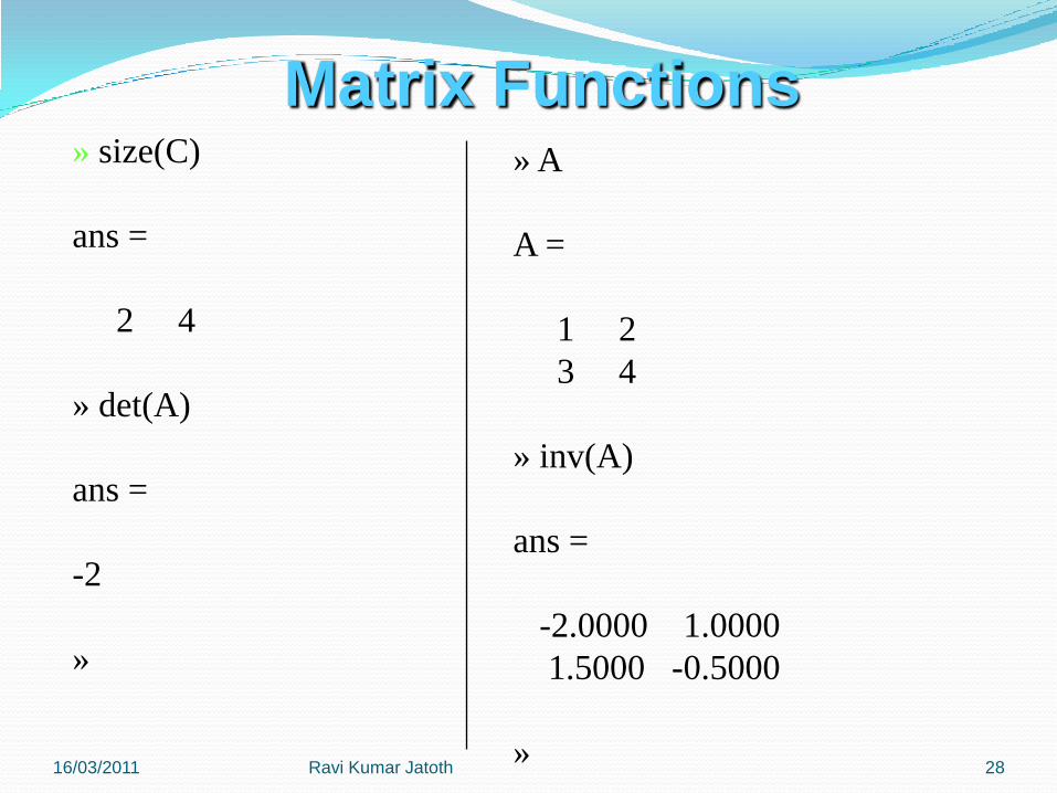
Matrix Functions» size(C)
ans =
2 4
» det(A)
ans =
-2
»
» A
A =
1 2
3 4
» inv(A)
ans =
-2.0000 1.0000
1.5000 -0.5000
» 16/03/2011 28Ravi Kumar Jatoth

Try the following.
X*B , B*X , pi*X , B^2 , X^2,X.^2 , Y=X’*X , Y^2, Y.^2,B.*B , B*B’ , B.*B’ ,sqrt(X) , exp(X) , cos(X)
1 2 3, 2 3
4 5 6B X
16/03/2011 29Ravi Kumar Jatoth
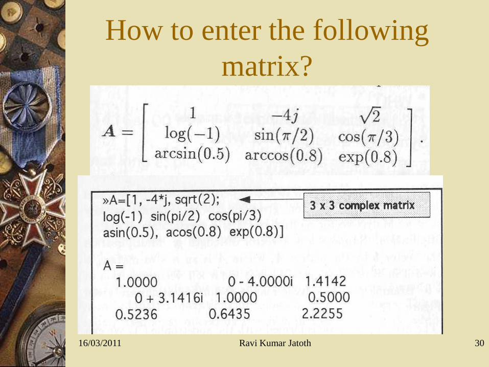
How to enter the following
matrix?
16/03/2011 30Ravi Kumar Jatoth
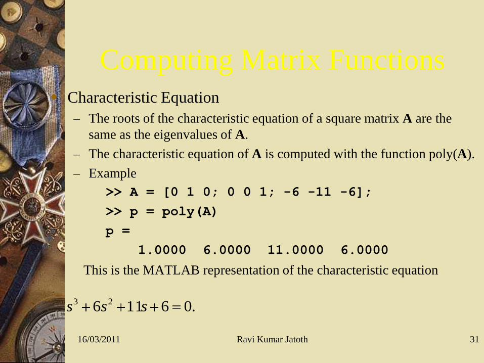
Computing Matrix Functions Characteristic Equation
– The roots of the characteristic equation of a square matrix A are the
same as the eigenvalues of A.
– The characteristic equation of A is computed with the function poly(A).
– Example
>> A = [0 1 0; 0 0 1; -6 -11 -6];
>> p = poly(A)
p =
1.0000 6.0000 11.0000 6.0000
This is the MATLAB representation of the characteristic equation
.06116 23 sss
16/03/2011 31Ravi Kumar Jatoth
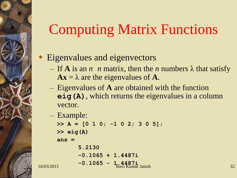
Computing Matrix Functions
Eigenvalues and eigenvectors
– If A is an n n matrix, then the n numbers λ that satisfy Ax = λ are the eigenvalues of A.
– Eigenvalues of A are obtained with the function eig(A), which returns the eigenvalues in a column vector.
– Example:>> A = [0 1 0; -1 0 2; 3 0 5];
>> eig(A)
ans =
5.2130
-0.1065 + 1.4487i
-0.1065 - 1.4487i16/03/2011 32Ravi Kumar Jatoth
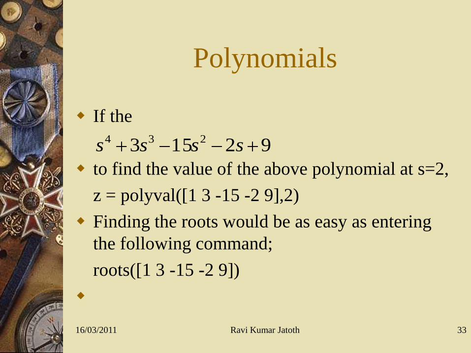
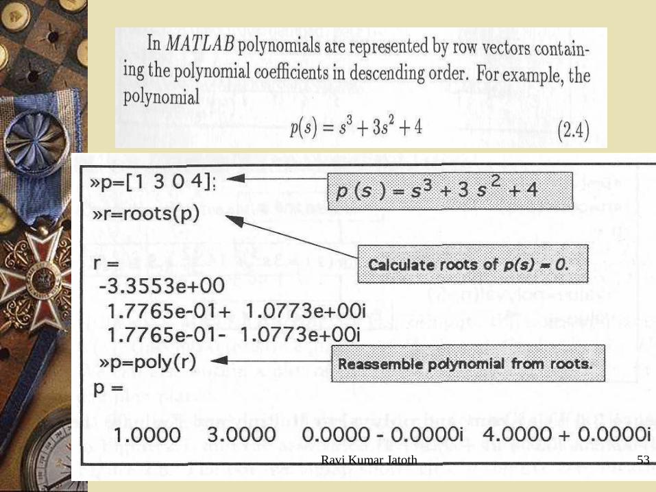
Polynomials
If the
to find the value of the above polynomial at s=2,
z = polyval([1 3 -15 -2 9],2)
Finding the roots would be as easy as entering
the following command;
roots([1 3 -15 -2 9])
92153 234 ssss
16/03/2011 33Ravi Kumar Jatoth
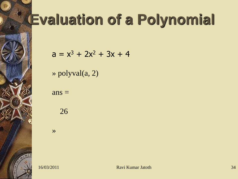
Evaluation of a Polynomial
a = x3 + 2x2 + 3x + 4
» polyval(a, 2)
ans =
26
»
16/03/2011 34Ravi Kumar Jatoth

Polynomial Multiplication
a = x3 + 2x2 + 3x + 4b = 4x2 + 9x + 16
» a = [1 2 3 4];
» b = [4 9 16];
» c = conv(a,b)
c =
4 17 46 75 84 64
»
16/03/2011 35Ravi Kumar Jatoth

Polynomial Curve Fitting
» x = [1 3 7 21];
» y = [2 9 20 55];
» polyfit(x,y,2)
ans =
-0.0251 3.1860 -0.8502
»
16/03/2011 36Ravi Kumar Jatoth
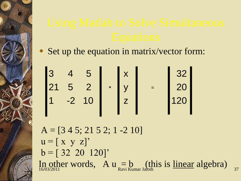
Using Matlab to Solve Simultaneous
Equations Set up the equation in matrix/vector form:
A = [3 4 5; 21 5 2; 1 -2 10]
u = [ x y z]’
b = [ 32 20 120]’
In other words, A u = b (this is linear algebra)
3 4 5
21 5 2
1 -2 10
x
y
z
*
32
20
120
=
16/03/2011 37Ravi Kumar Jatoth
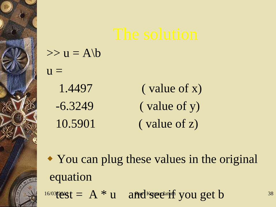
The solution>> u = A\b
u =
1.4497 ( value of x)
-6.3249 ( value of y)
10.5901 ( value of z)
You can plug these values in the original
equation
test = A * u and see if you get b16/03/2011 38Ravi Kumar Jatoth
16/03/2011
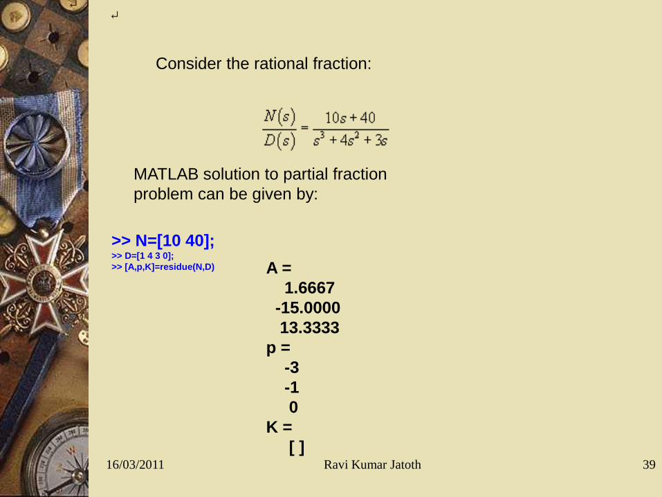
Consider the rational fraction:
MATLAB solution to partial fraction
problem can be given by:
>> N=[10 40]; >> D=[1 4 3 0];
>> [A,p,K]=residue(N,D) A =
1.6667
-15.0000
13.3333
p =
-3
-1
0
K =
[ ] 39Ravi Kumar Jatoth
Programming in MATLABScript files
A Script file contains a set of MATLAB
command
Use them when you have a long sequence
of statements to solve a problem
Can run the program by typing its name in
the command window or from tools in the
editor window.
16/03/2011 40Ravi Kumar Jatoth

for loops
General form:for index=initial: increment: limit
statements
end
s=0
for i=1:3:11
s=s+i
end
16/03/2011 41Ravi Kumar Jatoth

Example MATLAB program to find the roots of
1)cos(2)( xxf
% program 1 performs four iterations of
% Newton’s Method
X=.7
for i=1:4
X=X – (2*cos(X)-1)/(-2*sin(X))
end
X =1.1111
X =1.0483
X =1.0472
X =1.0472
Result
16/03/2011 42Ravi Kumar Jatoth

Final Thoughts
Nobody could or would want to know
everything about MATLAB.
Start with a particular project or problem.
Use the Help files.
Be willing to try something.
Be prepared for frustration, but if you need
MATLAB it is worth the frustration.
16/03/2011 43Ravi Kumar Jatoth
16/03/2011 44Ravi Kumar Jatoth
Control System Tool Box
16/03/2011 Ravi Kumar Jatoth 45

Example: Train system
we will consider a toy train consisting of an engine
and a car. Assuming that the train only travels in one
direction
we want to apply control to the train so that it has a
smooth start-up and stop, along with a constant-speed
ride.
16/03/2011 46Ravi Kumar Jatoth
Modeling cont..
The two are held together by a spring, which has the
stiffness coefficient of k
u, represents the coefficient of rolling friction
16/03/2011 47Ravi Kumar Jatoth

Free body diagram and Newton's
law
16/03/2011 48Ravi Kumar Jatoth

When finding the transfer function, zero initial
conditions must be assumed. The transfer function
should look like the one shown below.
16/03/2011 49Ravi Kumar Jatoth
Since MATLAB can not manipulate symbolic variables, let's
assign numerical values to each of the variables.
Let
M1 = 1 kg
M2 = 0.5 kg
k = 1 N/sec
F= 1 N
u = 0.002 sec/m
g = 9.8 m/s^2
16/03/2011 50Ravi Kumar Jatoth
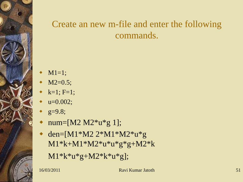
Create an new m-file and enter the following
commands.
M1=1;
M2=0.5;
k=1; F=1;
u=0.002;
g=9.8;
num=[M2 M2*u*g 1];
den=[M1*M2 2*M1*M2*u*g
M1*k+M1*M2*u*u*g*g+M2*k
M1*k*u*g+M2*k*u*g];
16/03/2011 51Ravi Kumar Jatoth

Transfer function
The transfer function can be of the
following form
16/03/2011 52Ravi Kumar Jatoth
16/03/2011 53Ravi Kumar Jatoth

16/03/2011 54Ravi Kumar Jatoth
The transfer function can be entered as
follows
G(s)=4(s+10)/(s+5)(s+15)
16/03/2011 55Ravi Kumar Jatoth

MATLAB code
num=4*[1 10];
den=conv([1 5],[1 15]);
printsys( num,den,’s’)
16/03/2011 56Ravi Kumar Jatoth

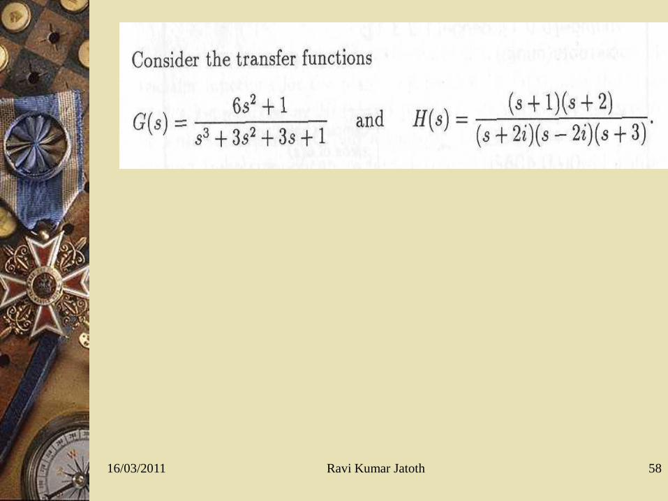
The function conv has been used to multiply
polynomials in the following MATLAB session for
the transfer function
16/03/2011
>> n1 = [5 1];
>> n2 = [15 1];
>> d1 = [1 0];
>> d2 = [3 1];
>> d3 = [10 1];
>> num = 100*conv(n1,n2);
>> den = conv(d1,conv(d2,d3));
>> GH = tf(num,den)
57Ravi Kumar Jatoth
16/03/2011 58Ravi Kumar Jatoth

16/03/2011 59Ravi Kumar Jatoth
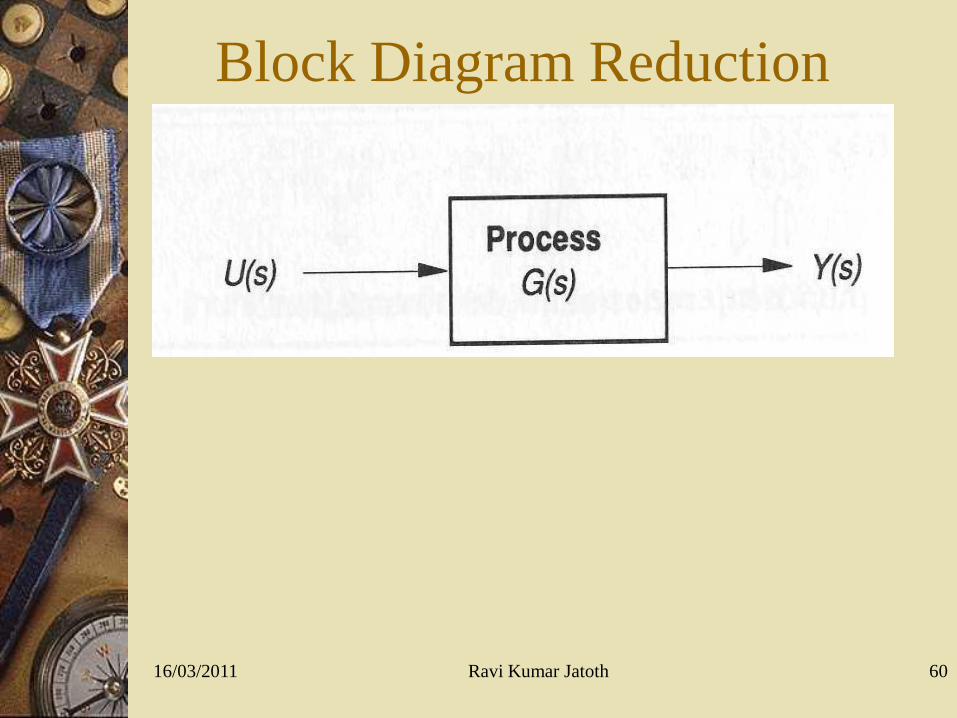
Block Diagram Reduction
16/03/2011 60Ravi Kumar Jatoth

Series Blocks
16/03/2011 Ravi Kumar Jatoth 61
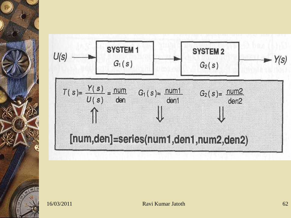
16/03/2011 62Ravi Kumar Jatoth

16/03/2011 63Ravi Kumar Jatoth
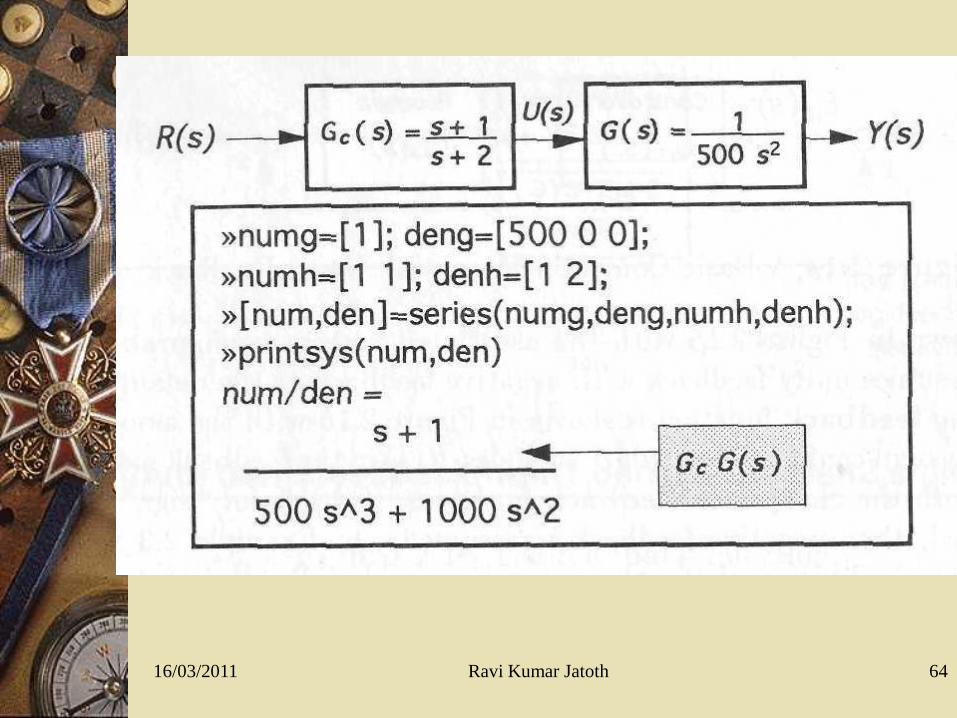
16/03/2011 64Ravi Kumar Jatoth
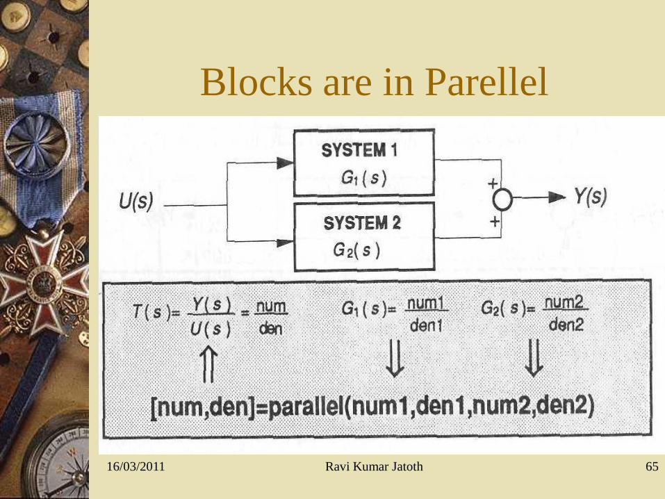
Blocks are in Parellel
16/03/2011 Ravi Kumar Jatoth 65
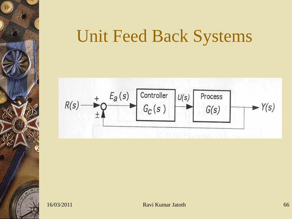
Unit Feed Back Systems
16/03/2011 Ravi Kumar Jatoth 66

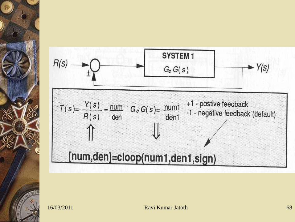
Building models
cloop : command provides a means of
generating a closed loop (unity feedback)
system description given an open loop
system .
Ex:
16/03/2011 67Ravi Kumar Jatoth
16/03/2011 68Ravi Kumar Jatoth

MATLAB code
ngo=[1 1];
dgo=conv([1 3],[1 5]);
[ngc2,dgc2]=cloop(ngo,dgo);
printsys(ngc2,dgc2,’s’)
16/03/2011 69Ravi Kumar Jatoth

16/03/2011 70Ravi Kumar Jatoth

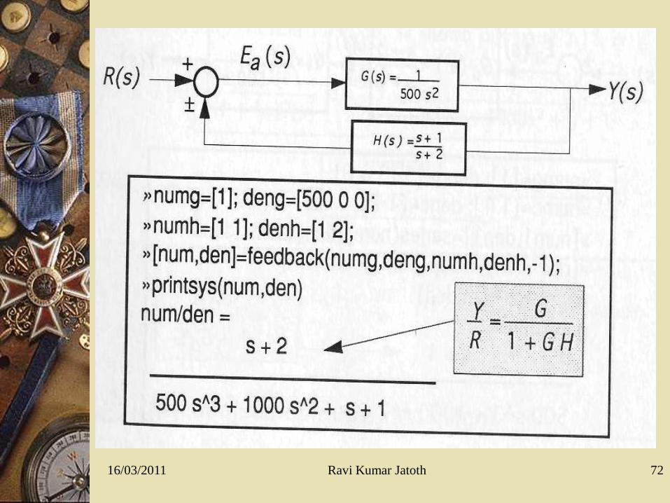
feedback
feedback: for non unity feedback use feed
back command.
Ex:
16/03/2011 71Ravi Kumar Jatoth
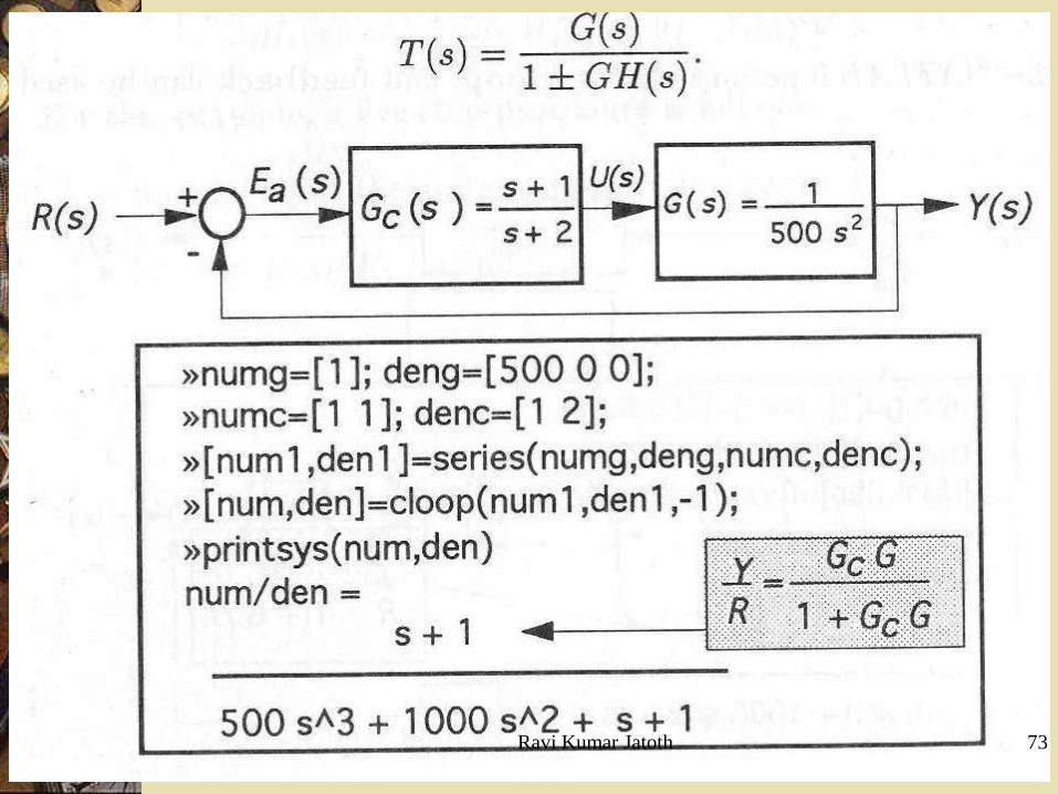
16/03/2011 72Ravi Kumar Jatoth
16/03/2011 73Ravi Kumar Jatoth
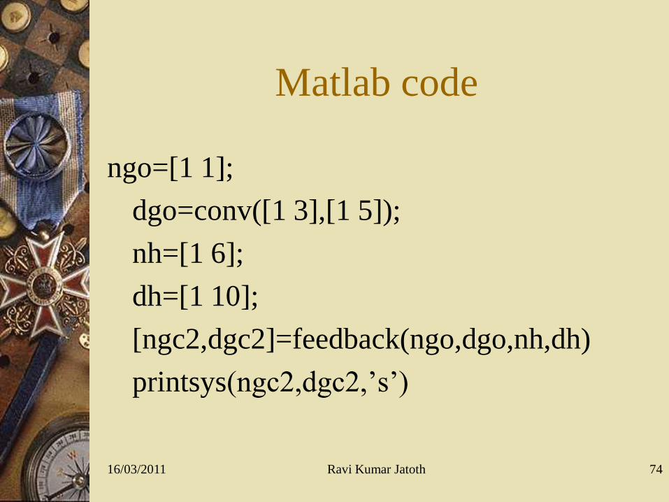
Matlab code
ngo=[1 1];
dgo=conv([1 3],[1 5]);
nh=[1 6];
dh=[1 10];
[ngc2,dgc2]=feedback(ngo,dgo,nh,dh)
printsys(ngc2,dgc2,’s’)
16/03/2011 74Ravi Kumar Jatoth

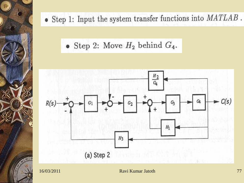
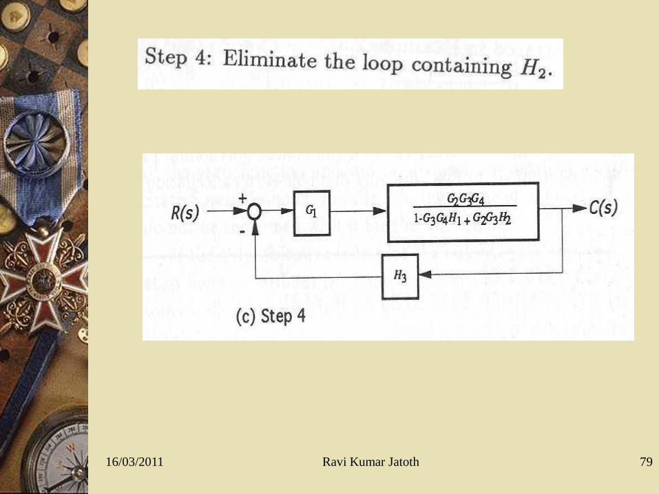
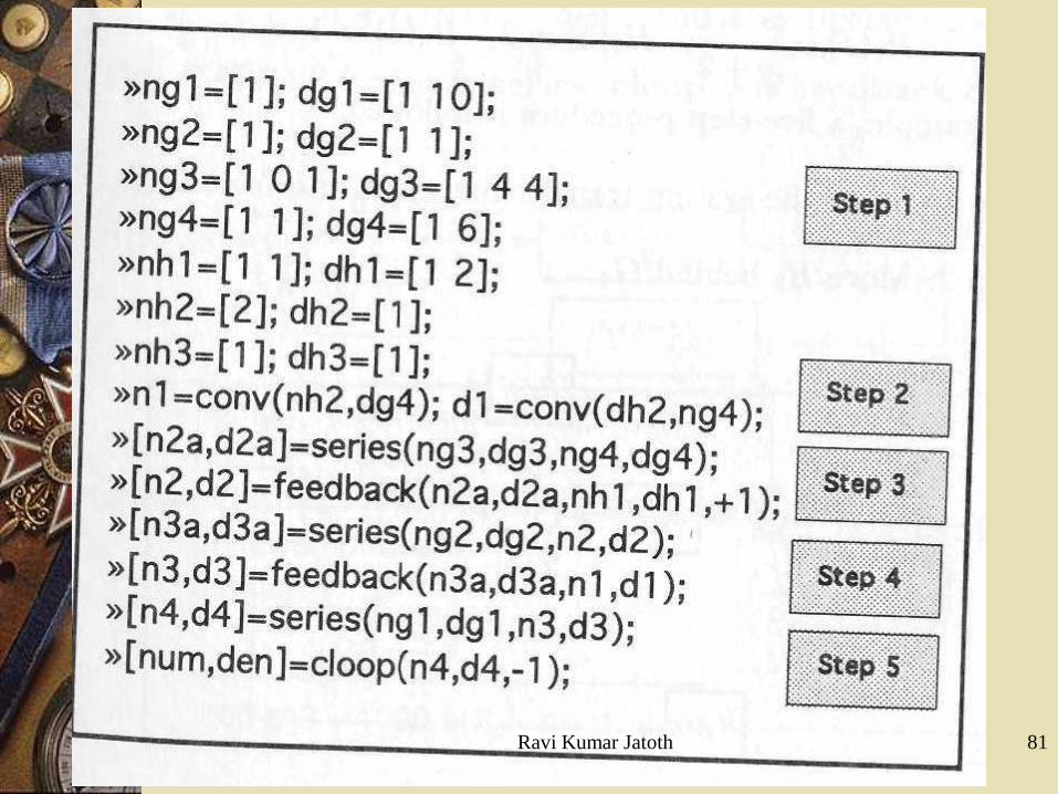
Block Diagram Reduction
16/03/2011 Ravi Kumar Jatoth 75

16/03/2011 76Ravi Kumar Jatoth
16/03/2011 77Ravi Kumar Jatoth

16/03/2011 78Ravi Kumar Jatoth
16/03/2011 79Ravi Kumar Jatoth

16/03/2011 80Ravi Kumar Jatoth
16/03/2011 81Ravi Kumar Jatoth

16/03/2011 82Ravi Kumar Jatoth
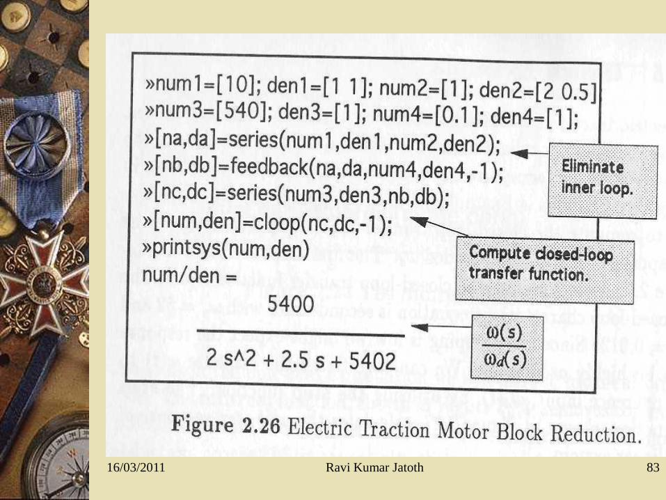
16/03/2011 83Ravi Kumar Jatoth
How to find out poles &zeros
G(s)=(5s^2+3s+4)/(s^3+2s^2+4s+7)
16/03/2011 84Ravi Kumar Jatoth

num=[5 3 4];
den=[1 2 4 7];
[z,p]=tf2zp(num,den)
16/03/2011 85Ravi Kumar Jatoth

Creating transfer function from
poles and zeroes
Zp2tf:
z=[0; 0; 0; -1];
p=[-1+i -1-i -2 -3.15+2.63*i
-3.15- 2.63*i];
k=2;
[num,den]=zp2tf(z,p,k);
printsys(num,den,'s')
16/03/2011 86Ravi Kumar Jatoth

Time Response Analysis
16/03/2011 Ravi Kumar Jatoth 87

Time Response of a system to
different inputs
System Response
Step and impulse responses of LTI objects can be obtained by the commands
step and impulse . For example, to obtain the step response of the system
represented in LTI object G, enter
16/03/2011
num = [1 1];
den = [1 3 1];
G = tf(num,den)
>> step(G)
88Ravi Kumar Jatoth
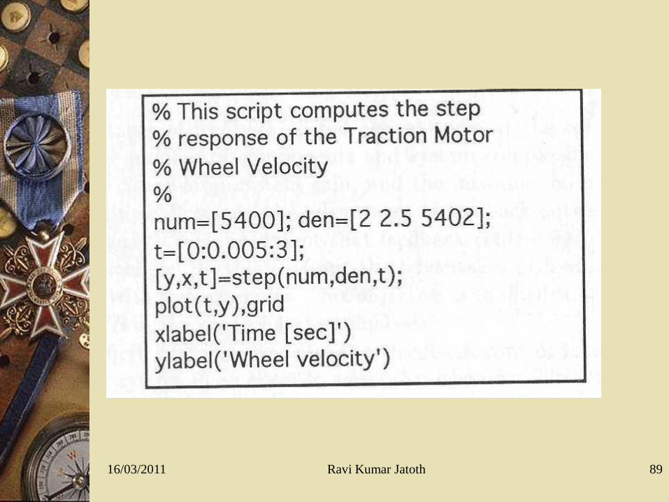
16/03/2011 89Ravi Kumar Jatoth

Display response to step input
G(s)=5/(s^2+3s+12)
num=5;
den=[1 3 12];
step(num,den)
16/03/2011 90Ravi Kumar Jatoth
Step and impulse response data can be
collected into MATLAB variables by using
two left hand arguments. For example, the
following commands will collect step and
impulse response amplitudes in yt and time
samples in t.
[yt, t] = step(G)
[yt, t] = impulse(G)16/03/2011 91Ravi Kumar Jatoth
Changing the magnitude of the step
step(100*num,den)
16/03/2011 92Ravi Kumar Jatoth
Specifying the time scale
step (num,den,t)
16/03/2011 93Ravi Kumar Jatoth

Saving the response
If the time vector is used, the command is:
[y,x] = step(num,den,4); If the time vector is not used, the command is:
16/03/2011 94Ravi Kumar Jatoth
Impulse Response
num=5;
den=[1 3 12];
impulse(num,den)
16/03/2011 95Ravi Kumar Jatoth

16/03/2011
Response of LTI systems to arbitrary inputs can be obtained by the
command lsim. The command lsim(G,u,t) plots the time response
of the LTI model G to the input signal described by u and t. The
time vector t consists of regularly spaced time samples and u is a
matrix with as many columns as inputs and whose ith -row specifies
the input value at time t(i). Observe the following MATLAB session
to obtain the time response of LTI system G to sinusoidal input of
unity magnitude.
>> t=0:0.01:7;
>> u=sin(t);
>> lsim(G,u,t)
96Ravi Kumar Jatoth
16/03/2011
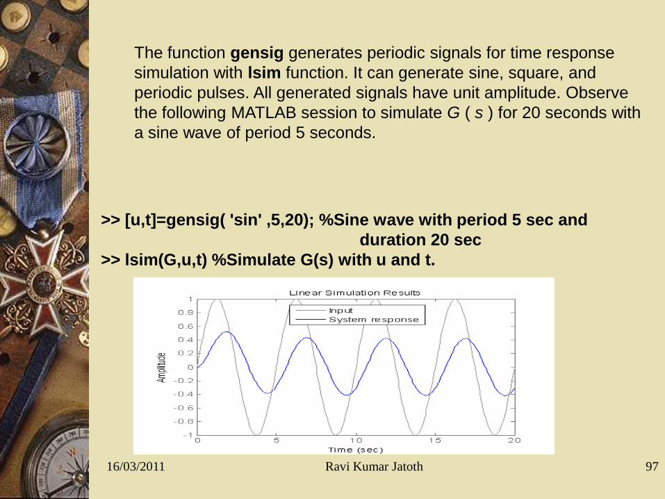
The function gensig generates periodic signals for time response
simulation with lsim function. It can generate sine, square, and
periodic pulses. All generated signals have unit amplitude. Observe
the following MATLAB session to simulate G ( s ) for 20 seconds with
a sine wave of period 5 seconds.
>> [u,t]=gensig( 'sin' ,5,20); %Sine wave with period 5 sec and
duration 20 sec
>> lsim(G,u,t) %Simulate G(s) with u and t.
97Ravi Kumar Jatoth

16/03/2011
The following MATLAB script calculates
the step response of second-order system
with and various values of t=[0:0.1:12]; num=[1];
zeta1=0.1; den1=[1 2*zeta1 1];
zeta2=0.2; den2=[1 2*zeta2 1];
zeta3=0.4; den3=[1 2*zeta3 1];
zeta4=0.7; den4=[1 2*zeta4 1];
zeta5=1.0; den5=[1 2*zeta5 1];
zeta6=2.0; den6=[1 2*zeta6 1];
[y1,x]=step(num,den1,t); [y2,x]=step(num,den2,t);
[y3,x]=step(num,den3,t); [y4,x]=step(num,den4,t);
[y5,x]=step(num,den5,t); [y6,x]=step(num,den6,t);
plot(t,y1,t,y2,t,y3,t,y4,t,y5,t,y6)
xlabel( 't' ), ylabel( 'y(t)' )
grid
98Ravi Kumar Jatoth
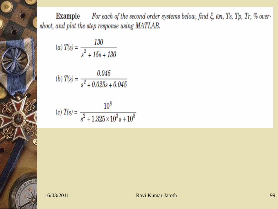
16/03/2011 Ravi Kumar Jatoth 99
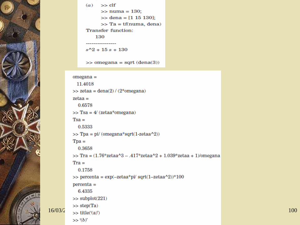
16/03/2011 Ravi Kumar Jatoth 100

16/03/2011 Ravi Kumar Jatoth 101

16/03/2011 Ravi Kumar Jatoth 102
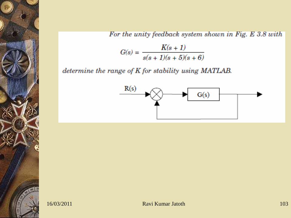
16/03/2011 Ravi Kumar Jatoth 103
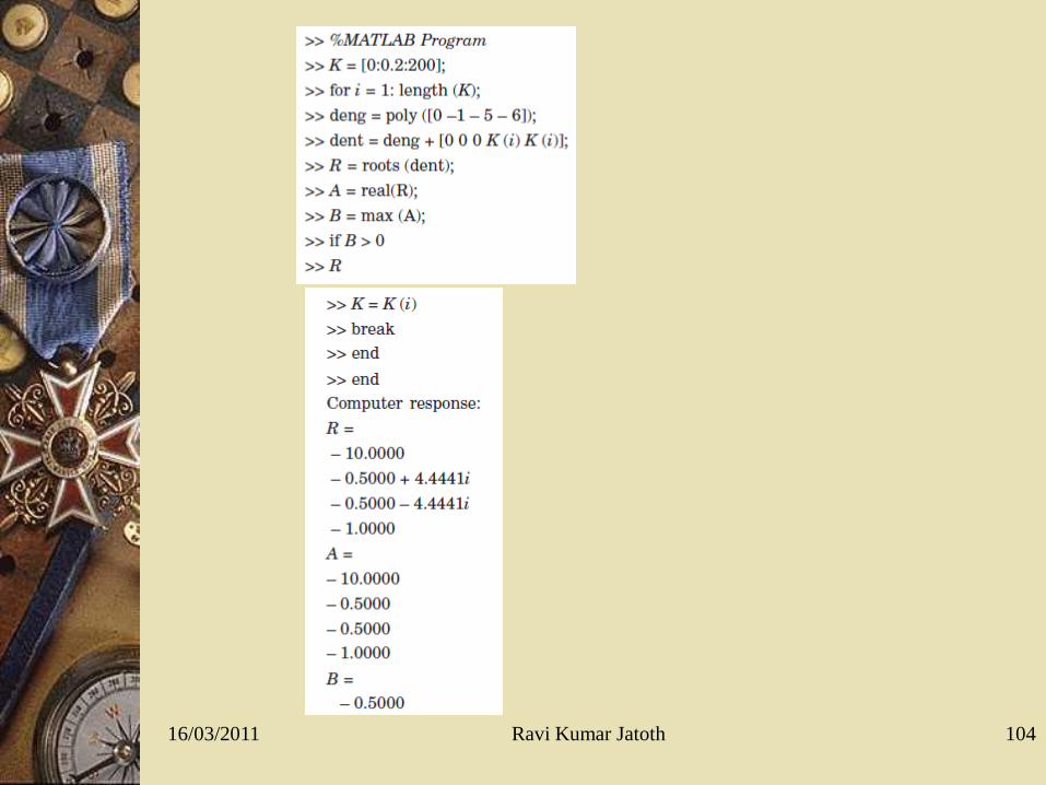
16/03/2011 Ravi Kumar Jatoth 104
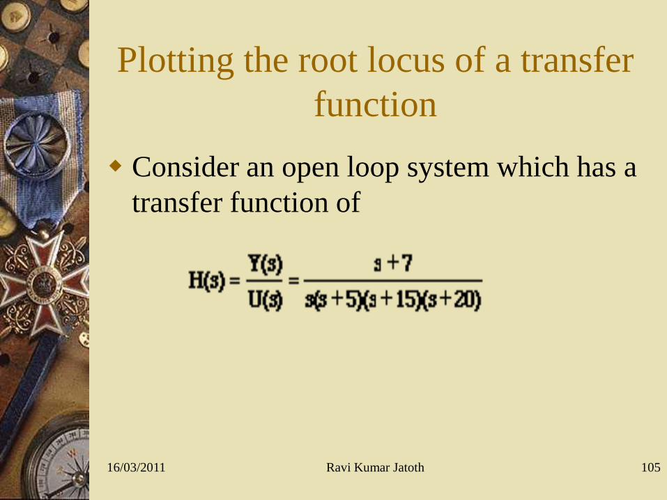
Plotting the root locus of a transfer
function
Consider an open loop system which has a
transfer function of
16/03/2011 105Ravi Kumar Jatoth
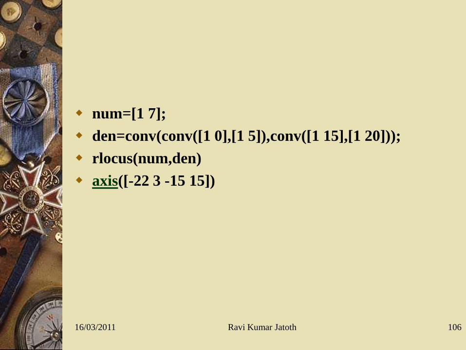
num=[1 7];
den=conv(conv([1 0],[1 5]),conv([1 15],[1 20]));
rlocus(num,den)
axis([-22 3 -15 15])
16/03/2011 106Ravi Kumar Jatoth

Choosing a value of K from the root locus
In our problem, we need an overshoot less than 5%
(which means a damping ratio Zeta of greater than
0.7) and a rise time of 1 second (which means a
natural frequency Wn greater than 1.8). Enter in the
Matlab command window:
zeta=0.7; Wn=1.8; sgrid(zeta, Wn)
16/03/2011 107Ravi Kumar Jatoth

16/03/2011 Ravi Kumar Jatoth 108
16/03/2011 Ravi Kumar Jatoth 109

16/03/2011 Ravi Kumar Jatoth 110

16/03/2011 Ravi Kumar Jatoth 111

16/03/2011 Ravi Kumar Jatoth 112

Frequency Response Analysis and
Design
The frequency response is a representation of the system's response to sinusoidal inputs at varying frequencies. The output of a linear system to a sinusoidal input is a sinusoid of the same frequency but with a different magnitude and phase. The frequency response is defined as the magnitude and phase differences between the input and output sinusoids. In this tutorial, we will see how we can use the open-loop frequency response of a system to predict its behavior in closed-loop. I
16/03/2011 113Ravi Kumar Jatoth

1.Bode plots
2.Gain and phase margin
16/03/2011 114Ravi Kumar Jatoth

code
50 /s^3 + 9 s^2 + 30 s + 40
bode(50,[1 9 30 40])
16/03/2011 115Ravi Kumar Jatoth

Gain and Phase Margin
Let's say that we have the following system:
where K is a variable (constant) gain and G(s) is the plant under
consideration. The gain margin is defined as the change in open
loop gain required to make the system unstable. Systems with
greater gain margins can withstand greater changes in system
parameters before becoming unstable in closed loop.
16/03/2011 116Ravi Kumar Jatoth
PHASE MARGIN
The phase margin is defined as the change in open loop phase shift required to make a closed loop system unstable.
The phase margin also measures the system's tolerance to time delay. If there is a time delay greater than 180/Wpc in the loop (where Wpc is the frequency where the phase shift is 180 deg), the system will become unstable in closed loop. The time delay can be thought of as an extra block in the forward path of the block diagram that adds phase to the system but has no effect the gain. That is, a time delay can be represented as a block with magnitude of 1 and phase w*time_delay (in radians/second).
16/03/2011 117Ravi Kumar Jatoth

16/03/2011 118Ravi Kumar Jatoth

16/03/2011 Ravi Kumar Jatoth 119
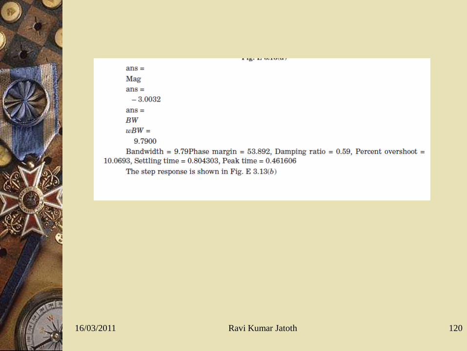
16/03/2011 Ravi Kumar Jatoth 120
SIMULINK
Simulink is started from the MATLAB
command prompt by entering the
following command:
simulink
16/03/2011 121Ravi Kumar Jatoth
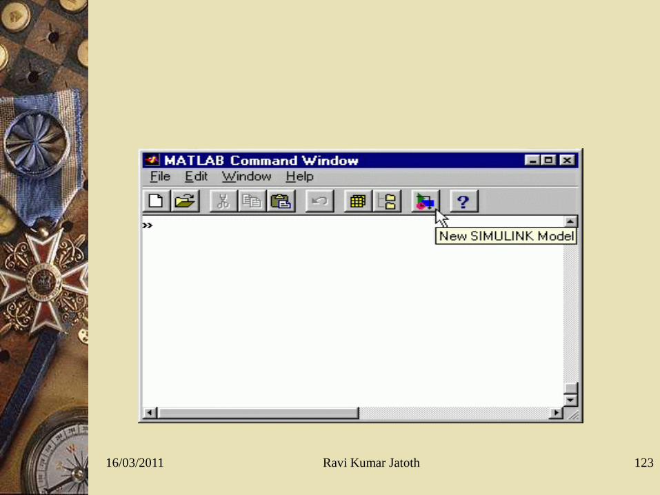
Alternatively, you can hit the New
Simulink Model button at the top of the
MATLAB command window as shown
below:
16/03/2011 122Ravi Kumar Jatoth
16/03/2011 123Ravi Kumar Jatoth

When it starts, Simulink brings up two windows. The first
is the main Simulink window, which appears as:
16/03/2011 124Ravi Kumar Jatoth
Blocks
There are several general classes of blocks:
Sources: Used to generate various signals
Sinks: Used to output or display signals
Discrete: Linear, discrete-time system elements (transfer functions, state-space models, etc.)
Linear: Linear, continuous-time system elements and connections (summing junctions, gains, etc.)
Nonlinear: Nonlinear operators (arbitrary functions, saturation, delay, etc.)
Connections: Multiplex, Demultiplex, System Macros, etc.
16/03/2011 125Ravi Kumar Jatoth
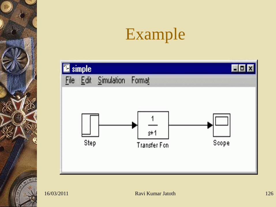
Example
16/03/2011 126Ravi Kumar Jatoth

Modifying Blocks
16/03/2011 127Ravi Kumar Jatoth
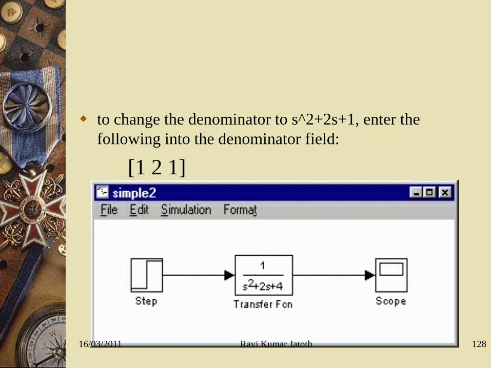
to change the denominator to s^2+2s+1, enter the
following into the denominator field:
[1 2 1]
16/03/2011 128Ravi Kumar Jatoth

The "step" block can also be double-clicked, bringing up
the following dialog box.
16/03/2011 129Ravi Kumar Jatoth

The most complicated of these three blocks is the "Scope"
block. Double clicking on this brings up a blank
oscilloscope screen
16/03/2011 130Ravi Kumar Jatoth
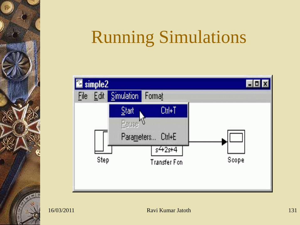
Running Simulations
16/03/2011 131Ravi Kumar Jatoth
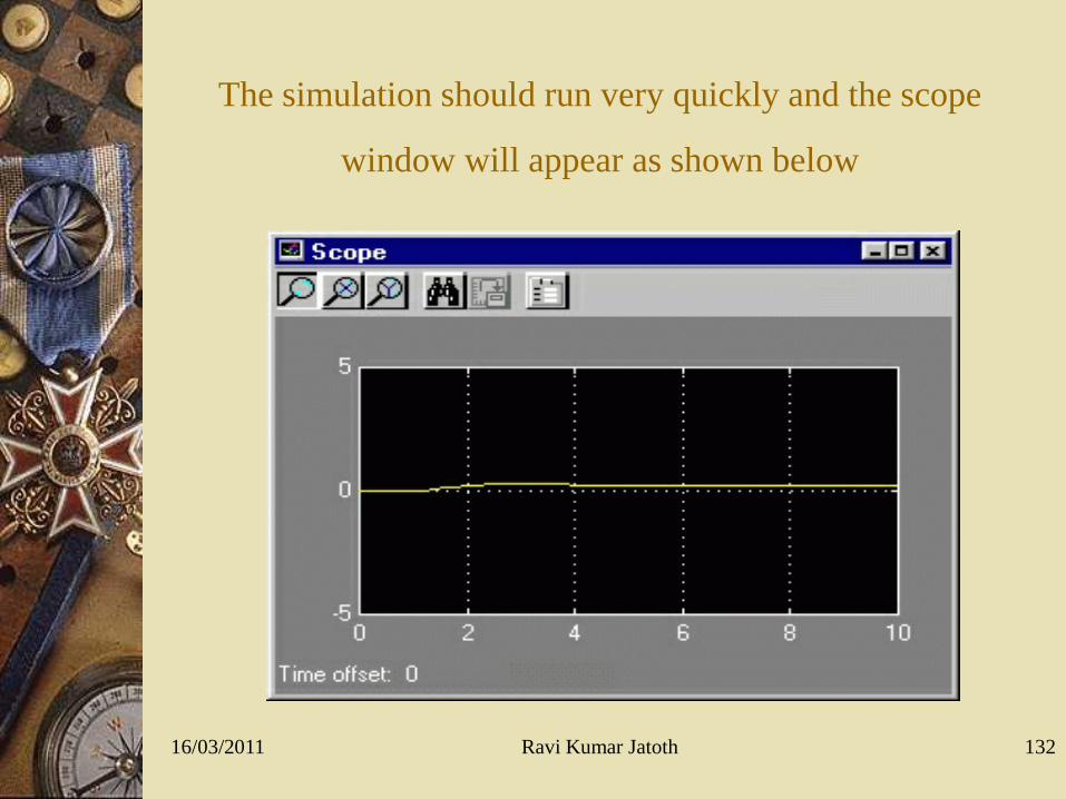
The simulation should run very quickly and the scope
window will appear as shown below
16/03/2011 132Ravi Kumar Jatoth
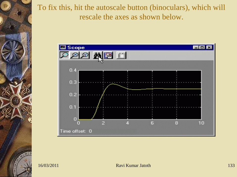
To fix this, hit the autoscale button (binoculars), which will
rescale the axes as shown below.
16/03/2011 133Ravi Kumar Jatoth

Thank you!
16/03/2011 134Ravi Kumar Jatoth

ALL THE BEST
16/03/2011 135Ravi Kumar Jatoth