Control and Design of MicrogridComponents

Final Project Report

Power Systems Engineering Research Center

A National Science FoundationIndustry/University Cooperative Research Center

since 1996

PSERC

Power Systems Engineering Research Center

Control and Design of Microgrid Components

Final Project Report

Report Authors

Robert H. Lasseter, Project Leader Paolo Piagi

University of Wisconsin-Madison

PSERC Publication 06-03

January 2006

Information about this project For information about this project contact: Professor Robert H. Lasseter: Department of Electrical and Computer Engineering University of Wisconsin-Madison 2546 Engineering Hall, 1415 Engineering Drive Madison, WI 53706 608-262-0186 lasseter@engr.wisc.edu Power Systems Engineering Research Center This is a project report from the Power Systems Engineering Research Center (PSERC). PSERC is a multi-university Center conducting research on challenges facing a restructuring electric power industry and educating the next generation of power engineers. More information about PSERC can be found at the Center’s website: http://www.pserc.org. For additional information, contact: Power Systems Engineering Research Center Cornell University 428 Phillips Hall Ithaca, New York 14853 Phone: 607-255-5601 Fax: 607-255-8871 Notice Concerning Copyright Material PSERC members are given permission to copy without fee all or part of this publication for internal use if appropriate attribution is given to this document as the source material. This report is available for downloading from the PSERC website.

©2006 Board of Regents, University of Wisconsin System. All rights reserved

i

Acknowledgements This is the final report for the Power Systems Engineering Research Center (PSERC) project “Microgrid Protection and Control” (project T-18). The authors express their appreciation for the support provided by the PSERC industrial members and by the National Science Foundation under grant NSF EEC-0119230 received from the Industry / University Cooperative Research Center program. This work was also supported in part by the California Energy Commission (500-03-024).

ii

Executive Summary

Economic, technology and environmental incentives are changing the face of electricity generation and transmission. Centralized generating facilities are giving way to smaller, more distributed generation partially due to the loss of traditional economies of scale. Distributed generation encompasses a wide range of prime mover technologies, such as internal combustion (IC) engines, gas turbines, microturbines, photovoltaic, fuel cells and wind-power. Most emerging technologies such as micro-turbines, photovoltaic, fuel cells and gas internal combustion engines with permanent magnet generator have an inverter to interface with the electrical distribution system. These emerging technologies have lower emissions, and have the potential to have lower cost, thus negating traditional economies of scale. The applications include power support at substations, deferral of T&D upgrades, and onsite generation. Penetration of distributed generation across the US has not yet reached significant levels. However, that situation is changing rapidly and requires attention to issues related to high penetration of distributed generation within the distribution system. Indiscriminant application of individual distributed generators can cause as many problems as it may solve. A better way to realize the emerging potential of distributed generation is to take a system approach which views generation and associated loads as a subsystem or a “microgrid”. This approach allows for local control of distributed generation thereby reducing or eliminating the need for central dispatch. During disturbances, the generation and corresponding loads can separate from the distribution system to isolate the microgrid’s load from the disturbance (and thereby maintaining high level of service) without harming the transmission grid’s integrity. Intentional islanding of generation and loads has the potential to provide a higher local reliability than that provided by the power system as a whole. The size of emerging generation technologies permits generators to be placed optimally in relation to heat loads allow for use of waste heat. Such applications can more than double the overall efficiencies of the systems. Most current microgrid implementations combine loads with sources, allow for intentional islanding, and try to use the available waste heat. These solutions rely on complex communication and control, and are dependent on key components and require extensive site engineering. The objective of this work is to provide these features without a complex control system requiring detailed engineering for each application. Our approach is to provide generator-based controls that enable a plug-and-play model without communication or custom engineering for each site. Each innovation embodied in the microgrid concept (i.e., intelligent power electronic interfaces, and a single, smart switch for grid disconnect and resynchronization) was created specifically to lower the cost and improve the reliability of smaller-scale distributed generation systems (i.e., systems with installed capacities in the 10’s and 100’s of kW). The goal is to accelerate realization of the many benefits offered by smaller-scale DG, such as their ability to supply waste heat at the point of need (avoiding extensive thermal distribution networks) or to provide higher power quality to some but not all loads within a facility. From a grid perspective, the microgrid concept is attractive because it recognizes the reality that the nation’s distribution

iii

system is extensive, old, and will change only very slowly. The microgrid concept enables high penetration of DG without requiring re-design or re-engineering of the distribution system itself. To achieve this, we promote autonomous control in a peer-to-peer and plug-and-play operation model for each component of the microgrid. The peer-to-peer concept insures that there are no components, such as a master controller or central storage unit that is critical for operation of the microgrid. This implies that the microgrid can continue operating with loss of any component or generator. With one additional source (N+1) we can insure complete functionality with the loss of any source. Plug-and-play implies that a unit can be placed at any point on the electrical system without re-engineering the controls. The plug-and-play model facilitates placing generators near the heat loads thereby allowing more effective use of waste heat without complex heat distribution systems such as steam and chilled water pipes. The microgrid has two critical components, the static switch and the microsource. The static switch has the ability to autonomously island the microgrid from disturbances such as faults, IEEE 1547 events, or power quality events. After islanding, the reconnection of the microgrid is achieved autonomously after the tripping event is no longer present. This synchronization is achieved by using the frequency difference between the islanded microgrid and the utility grid insuring a transient free operation without having to match frequency and phase angles at the connection point. Each microsource can seamlessly balance the power on the islanded microgrid using a power vs. frequency droop controller. This frequency droop also insures that the microgrid frequency is different from the grid to facilitate reconnection to the utility. This report documents the challenges, problems, and solutions that provide for these important features. The solutions have been fully simulated on software models to test their quality. Then, the control design has been digitally implemented on a hardware setup with two sources here at the University of Wisconsin-Madison, confirming all the theoretical results. With support from the California Energy Commission, a full-scale microgrid will be tested at AEP’s Dolan facility midyear of 2006.

iv

Table of Contents

Chapter 1. Introduction ................................................................................................................. 1 1.1 Emerging Generation Technologies................................................................................................ 1

1.2 Issues and Benefits Related to Emerging Generation Technologies ............................................ 2 1.2.1 Control......................................................................................................................................... 2 1.2.2 Operation and Investment ........................................................................................................... 3 1.2.3 Optimal Location for Heating/Cooling Cogeneration ................................................................. 3 1.2.4 Power Quality/ Power Management/ Reliability......................................................................... 3

1.3 Microgrid Concept ........................................................................................................................... 4 1.3.1 Unit Power Control Configuration .............................................................................................. 5 1.3.2 Feeder Flow Control Configuration ............................................................................................ 6 1.3.3 Mixed Control Configuration...................................................................................................... 6

Chapter 2. Static Switch................................................................................................................. 7 2.1 Direction of Current at Synchronization........................................................................................ 7

2.2 Direction of Current at Steady State .............................................................................................. 8

2.3 Synchronization Conditions........................................................................................................... 11

Chapter 3. Microsource Details................................................................................................... 19 3.1 Microsource Controller.................................................................................................................. 19

3.1.1 P and Q Calculation................................................................................................................... 21 3.1.2 Voltage Magnitude Calculation................................................................................................. 22 3.1.3 Voltage Control ......................................................................................................................... 24 3.1.4 Q versus E Droop ...................................................................................................................... 24 3.1.5 P versus Frequency Droop ........................................................................................................ 26

3.2 Power Control Mode with Limits on Unit Power ........................................................................ 28 3.2.1 Steady State Characteristics with Output Power Control.......................................................... 29 3.2.2 Steady State Characteristics with Feeder Flow Control ............................................................ 38 3.2.3 Mixed System............................................................................................................................ 47

Chapter 4. Interface of Inverter to Local System ....................................................................... 50 4.1 Prime Mover Dynamics and Ratings ............................................................................................ 50

4.2 DC Bus and Storage Ratings ......................................................................................................... 52

4.3 Sizing the Coupling Inductor, Inverter Voltage and Power Angle ............................................ 53 4.3.1 P versus Q Area of Operation.................................................................................................... 55

4.4 System Ratings................................................................................................................................ 59

Chapter 5. Unbalanced Systems .................................................................................................. 64 5.1 Reasons that Determine Unbalance .............................................................................................. 64

5.2 Unbalance Correction .................................................................................................................... 65

v

Table of Contents (continued)

5.3 Operation Under Unbalance.......................................................................................................... 65

Chapter 6. Hardware Implementation ........................................................................................ 72 6.1 Basic System.................................................................................................................................... 72

6.2 Description of the Laboratory System.......................................................................................... 73 6.2.1 Transformers ............................................................................................................................. 74 6.2.2 Cables ........................................................................................................................................ 75 6.2.3 Loads ......................................................................................................................................... 78

6.3 Control Implementation................................................................................................................. 83

6.4 Gate Pulse Implementation with Space Vector Modulation....................................................... 85

Chapter 7. Microgrid Tests .......................................................................................................... 91 7.1 Choice of Setpoints for the Series Configuration......................................................................... 93

7.2 Grid Fluctuations............................................................................................................................ 99

7.3 Series Configuration..................................................................................................................... 101 7.3.1 Unit 1 (P), Unit 2 (P), Import from Grid ................................................................................. 102 7.3.2 Unit 1 (P), Unit 2 (P), Export to Grid...................................................................................... 112 7.3.3 Unit 1 (F), Unit 2 (F), Import from Grid ................................................................................. 122 7.3.4 Unit 1 (F), Unit 2 (F), Export to Grid...................................................................................... 136 7.3.5 Unit 1 (F), Unit 2 (P), Import from Grid ................................................................................. 146 7.3.6 Unit 1 (F), Unit 2 (P), Export to Grid...................................................................................... 160 7.3.7 Unit 1 (P), Unit 2 (F), Import from Grid ................................................................................. 170 7.3.8 Unit 1 (P), Unit 2 (F), Export to Grid...................................................................................... 184

7.4 Parallel Configuration.................................................................................................................. 194 7.4.1 Unit 1 (F), Unit 2 (F), Import from Grid ................................................................................. 195 7.4.2 Unit 1 (F), Unit 2 (F), Export to Grid...................................................................................... 209 7.4.3 Unit 1 (F), Unit 2 (P), Import from Grid ................................................................................. 219 7.4.4 Unit 1 (F), Unit 2 (P), Export to Grid...................................................................................... 233

Chapter 8. Conclusions.............................................................................................................. 243

REFERENCES………………………………………………………………………………...244

vi

List of Figures Figure 1.1 Microgrid Architecture Diagram.................................................................................. 5 Figure 2.1 Current Direction as the Switch is Closed.................................................................... 8 Figure 2.2 Power vs. Frequency Droop. ........................................................................................ 9 Figure 2.3 Island Connection of Two Microsources, A has Higher Frequency than B................. 9 Figure 2.4 Island Connection of Two Microsources, A has Lower Frequency than B. .............. 10 Figure 2.5 Receding Trajectory of Voltage Vector V.................................................................. 11 Figure 2.6 Voltages on Either Side and Across the Static Switch. .............................................. 12 Figure 2.7 Three Phase Currents of the Static Switch, with Condition (ii) not Met.................... 13 Figure 2.8 Switch Voltage and Microsource Current, with Condition (ii) not Met..................... 14 Figure 2.9 Microsource Power Injection and Frequency, with Condition (ii) not Met. .............. 14 Figure 2.10 Voltage Vector Plane Showing Correct Reclose Timing. ........................................ 15 Figure 2.11 Three Phase Currents of the Static Switch, with Condition (ii) Met........................ 16 Figure 2.12 Switch Voltage and Microsource Current, with Condition (ii) Met......................... 16 Figure 2.13 Microsource Power Injection and Frequency, with Condition (ii) Met. .................. 17 Figure 2.14 Voltage Across the Static Switch During Synchronization, 1sec/div, 200V/div. .... 18 Figure 2.15 Grid and Microsource Current During Synchronization, 100ms/div, 10A/div. ....... 18 Figure 3.1 Microsource Diagram................................................................................................. 19 Figure 3.2 Final Version of Microsource Control. ...................................................................... 20 Figure 3.3 P and Q Calculation Blocks........................................................................................ 21 Figure 3.4 Voltage Magnitude Calculation Block. ...................................................................... 22 Figure 3.5 Selective Filter Diagram............................................................................................. 23 Figure 3.6 Selective Filter Response. .......................................................................................... 23 Figure 3.7 Voltage Control Block................................................................................................ 24 Figure 3.8 Q versus Load Voltage, E, Droop Block.................................................................... 25 Figure 3.9 Q versus Load Voltage, E, Droop Characteristic. ...................................................... 26 Figure 3.10 Power – Frequency Droop Characteristic................................................................. 27 Figure 3.11 Block Diagram of the Active Power Droop. ............................................................ 27 Figure 3.12 Microsource Elements: Prime Mover, Storage, Inverter.......................................... 28 Figure 3.13 Diagram of a Unit Regulating Output Active Power. .............................................. 30 Figure 3.14 Unit Power Configuration. ....................................................................................... 31 Figure 3.15 Steady State P-ω Characteristics with Fixed, Minimum Slope................................ 32 Figure 3.16 Effectively Limiting Pmax on Output Power Control.............................................. 33 Figure 3.17 Effectively Limiting Pmin=0 on Output Power Control. ......................................... 35 Figure 3.18 Offset Generation to Limit Max Power with Integral Block.................................... 36 Figure 3.19 Offset Generation to Limit Minimum Power with Integral Block. .......................... 37 Figure 3.20 Control Diagram to Enforce Limits with Unit Power Control. ................................ 38 Figure 3.21 Diagram of a Unit Regulating Feeder Power Flow. ................................................. 39 Figure 3.22 Load Tracking Configuration. .................................................................................. 40 Figure 3.23 Steady State Characteristics on the F-ω Droop with Feeder Flow Control.............. 41 Figure 3.24 Single (a), and Multiple (b) Feeders Source Connectivity. ...................................... 42 Figure 3.25 Sliding Window of Unit Power Limits..................................................................... 43 Figure 3.26 Steady State Characteristics for (a) P=0 Limit and (b) P=Pmax Limit. ................... 45 Figure 3.27 Steady State Characteristic Including Limits on the F-ω Plane with Feeder Flow

Control. ................................................................................................................................. 45

vii

List of Figures (continued) Figure 3.28 Control Diagram to Enforce Limits with Feeder Flow Control. .............................. 46 Figure 3.29 Characteristics on the ”Regulated Power vs. ω” Plane for a Mixed System............ 47 Figure 3.30 Mixed System on a Single Feeder, with Flow Control Near the Utility. ................. 48 Figure 3.31 Steady State Characteristics Including Limits on the Regulated Power vs. Frequency

Plane, with a Mixed System.................................................................................................. 49 Figure 4.1 Microsource Component Parts. .................................................................................. 50 Figure 4.2 Capstone DC Bus Voltage During Load Changes in Island Mode. ........................... 51 Figure 4.3 Fuel Cell Stack Voltage as a Function of the Output Current. ................................... 52 Figure 4.4 Replacement of Prime Mover + DC Storage with DC Source................................... 53 Figure 4.5 P and Q as a Function of the Voltages and their Angles. ........................................... 54 Figure 4.6 Power-Angle Characteristic........................................................................................ 54 Figure 4.7 P and Q Plane Capability with Constant Voltage and Impedance. ............................ 56 Figure 4.8 P and Q Plane Capability with Constant Voltage and Angle X=0.2 pu. .................... 57 Figure 4.9 P and Q Plane Capability with Constant Voltage and Angle X=0.1 pu. .................... 58 Figure 4.10 Voltage Source Inverter............................................................................................ 59 Figure 4.11 AC and DC Currents on the Voltage Sourced Inverter. ........................................... 61 Figure 4.12 Transformer Current During Fault on a) Wye Side, b) Delta Side. ......................... 62 Figure 5.1 Filter Gain as a Function of Frequency. ..................................................................... 66 Figure 5.2 P, Q and Magnitude of V. [50ms/div] ........................................................................ 67 Figure 5.3 Load Line to Line Voltages, 100V/div (upper traces) and Unit Currents, 10A/div

(lower traces). [20ms/div]..................................................................................................... 68 Figure 5.4 Load Line to Line Voltages (upper traces) and Unit Currents (lower traces). [1s/div]

............................................................................................................................................... 68 Figure 5.5 Unit 1 - Two Units in Parallel. [50ms/div]................................................................. 69 Figure 5.6 Unit 2- Two Units in Parallel. [50ms/div].................................................................. 70 Figure 5.7 One Unit Connected to the Grid. [50ms/div] ............................................................. 71 Figure 6.1 Single Phase Test System Diagram............................................................................ 72 Figure 6.2 Single Phase Diagram of Inverter Connection to the Feeder. .................................... 73 Figure 6.3 Single Phase Laboratory Circuit Diagram.................................................................. 74 Figure 6.4 The Active Power versus Frequency Droop............................................................... 80 Figure 6.5 Voltage Profile in the Microgrid without Microsources. ........................................... 81 Figure 6.6 Q versus E Droop. ...................................................................................................... 82 Figure 6.7 DSP Peripherals.......................................................................................................... 84 Figure 6.8 Interrupt Routine Queue. ............................................................................................ 85 Figure 6.9 Inverter Switch Topology........................................................................................... 86 Figure 6.10 Voltage Control Blocks, Hardware with Space Vector Modulation. ....................... 86 Figure 6.11 Achievable Voltage Vectors and Desired Voltage Vector. ...................................... 87 Figure 6.12 Voltage Partition on the Inverter Legs. .................................................................... 88 Figure 6.13 Gate Pulse Generator Block for Space Vector Modulation...................................... 90 Figure 7.1 Series (a) and Parallel (b) Circuit Configurations. ..................................................... 91 Figure 7.2 Series Configuration Diagram.................................................................................... 94 Figure 7.3 Control of P1 and P2, Unit Power. ............................................................................. 95 Figure 7.4 Control of P1 and P2, Feeder Flow. ........................................................................... 96 Figure 7.5 Control of F1 and F2, Unit Power. ............................................................................. 96

viii

List of Figures (continued) Figure 7.6 Control of F1 and F2, Feeder Flow. ........................................................................... 97 Figure 7.7 Control of F1 and P2, Unit Power. ............................................................................. 97 Figure 7.8 Control of F1 and P2, Feeder Flow. ........................................................................... 98 Figure 7.9 Control of P1 and F2, Unit Power. ............................................................................. 98 Figure 7.10 Control of P1 and F2, Feeder Flow. ......................................................................... 99 Figure 7.11 Actual Grid Frequency Samples............................................................................. 100 Figure 7.12 Impact on the Power Setpoint of a Frequency Deviation of 0.05 Hz..................... 100 Figure 7.13 Units in Series Configuration. ................................................................................ 101 Figure 7.14 Units in Parallel Configuration............................................................................... 194

ix

List of Tables Table 6.1 Transformer Data Summary. ....................................................................................... 75 Table 6.2 Cable Data Summary. .................................................................................................. 78 Table 6.3 Load Data Summary. ................................................................................................... 79 Table 6.4 Summary of Microsource Data.................................................................................... 83 Table 6.5 Lookup Table for Switching Positions. ....................................................................... 89 Table 7.1 Summary of Experiments for Each Group of Tests..................................................... 93 Table 7.2 Series Configuration Control Combinations. Importing from Grid. ........................... 95

1

Chapter 1. Introduction

Distributed generation (DG) encompasses a wide range of prime mover technologies, such as internal combustion (IC) engines, gas turbines, microturbines, photovoltaic, fuel cells and wind-power.

Penetration of distributed generation across the US has not yet reached significant levels. However that situation is changing rapidly and requires attention to issues related to high penetration of distributed generation within the distribution system. A better way to realize the emerging potential of distributed generation is to take a system approach which views generation and associated loads as a subsystem or a “microgrid”.

The CERTS microgrid concept is an advanced approach for enabling integration of, in principle, an unlimited quantity of distributed energy resources into the electricity grid. The microgrid concept is driven by two fundamental principles:

1) A systems perspective is necessary for customers, utilities, and society to capture the full benefits of integrating distributed energy resources into an energy system;

2) The business case for accelerating adoption of these advanced concepts will be driven, primarily, by lowering the first cost and enhancing the value of microgrids.

Each innovation embodied in the microgrid concept (i.e., intelligent power electronic interfaces, and a single, smart switch for grid disconnect and resynchronization) was created specifically to lower the cost and improve the reliability of smaller-scale distributed generation (DG) systems (i.e., systems with installed capacities in the 10’s and 100’s of kW). The goal of this work is to accelerate realization of the many benefits offered by smaller-scale DG, such as their ability to supply waste heat at the point of need (avoiding extensive thermal distribution networks) or to provide higher power quality to some but not all loads within a facility. From a grid perspective, the microgrid concept is attractive because it recognizes the reality that the nation’s distribution system is extensive, old, and will change only very slowly. The microgrid concept enables high penetration of DER without requiring re-design or re-engineering of the distribution system, itself.

During disturbances, the generation and corresponding loads can autonomously separate from the distribution system to isolate the microgrid’s load from the disturbance (and thereby maintaining high level of service) without harming the transmission grid’s integrity. Intentional islanding of generation and loads has the potential to provide a higher local reliability than that provided by the power system as a whole. The smaller size of emerging generation technologies permits generators to be placed optimally in relation to heat loads allowing for use of waste heat. Such applications can more than double the overall efficiencies of the systems.

1.1 Emerging Generation Technologies

In terms of the currently available technologies, the microsources can include fuel cells, renewable generation, as wind turbines or PV systems, microturbines and inverter based internal combustion generator set with inverters. One of the most promising applications of this new concept corresponds to the combined heat and power – CHP – applications leading to an increase of the overall energy effectiveness of the whole system.

2

Most emerging technologies such as micro-turbines, photovoltaic, fuel cells and gas internal combustion engines with permanent magnet generator require an inverter to interface with the electrical distribution system.

Photovoltaic and wind-power are important renewable technologies that require an inverter to interface with the electrical distribution system. The major issue with these technologies is the nature of the generation. The availability of their energy source is driven by weather, not the loads of the systems. These technologies can be labeled as intermittent and ideally they should be operated at maximum output. Intermittent sources can be used in the CERTS microgrid as a “negative load”, but not as a dispatchable source.

1.2 Issues and Benefits Related to Emerging Generation Technologies

1.2.1 Control A basic issue for distributed generation is the technical difficulties related to control of a significant number of microsources. For example for California to meet its DG objective it is possible that this could result in as many as 120,000, 100kW generators on their system. This issue is complex but the call for extensive development in fast sensors and complex control from a central point provides a potential for greater problems. The fundamental problem with a complex control system is that a failure of a control component or a software error will bring the system down. DG needs to be able to respond to events autonomous using only local information. For voltage drops, faults, blackouts etc. the generation needs to switch to island operation using local information. This will require an immediate change in the output power control of the micro-generators as they change from a dispatched power mode to one controlling frequency of the islanded section of network along with load following.

We believe that while some emerging control technologies are useful, the traditional power system provides important insights. Key power system concepts can be applied equally well to DG operation. For example the power vs. frequency droop and voltage control used on large utility generators can also provide the same robustness to systems of small DGs. From a communication point of view only the steady state power and voltage needs to be dispatched to optimize the power flow.

The area of major difference from utility generation is the possibility that inverter based DG cannot provide the instantaneous power needs due to lack of a large rotor. In isolated operation, load-tracking problems arise since micro-turbines and fuel cells have slow response to control signals and are inertia-less. A system with clusters of microsources designed to operate in an island mode requires some form of storage to ensure initial energy balance. The necessary storage can come in several forms; batteries or supercapacitors on the dc bus for each micro source; direct connection of ac storage devices (AC batteries; flywheels, etc, including inverters). The CERTS microgrid uses dc storage on each source’s dc bus to insure highest levels of reliability. In this situation one additional source (N+1) we can insure complete functionality with the loss of any component. This is not the case if there is a single ac storage device for the microgrid.

3

1.2.2 Operation and Investment The economy of scale favors larger DG units over microsources. For a microsource the cost of the interconnection protection can add as much as 50% to the cost of the system. DG units with a rating of three to five times that of a microsource have a connection cost much less per kWatt since the protection cost remain essentially fixed. The microgrid concept allows for the same cost advantage of large DG units by placing many microsources behind a single interface to the utility.

Using DG to reduce the physical and electrical distance between generation and loads can contribute to improvement in reactive support and enhancement to the voltage profile, removal of distribution and transmission bottlenecks, reduce losses, enhance the possibly of using waste heat and postpone investments in new transmission and large scale generation systems.

Contribution for the reduction of the losses in the European electricity distribution systems will be a major advantage of microsources. Taking Portugal as an example, the losses at the transmission level are about 1.8 to 2 %, while losses at the HV and MV distribution grids are about 4%. This amounts to total losses of about 6% excluding the LV distribution network. In 1999 Portugal’s consumption at the LV level was about 18 TWh. This means that with a large integration of microsources, say 20% of the LV load, a reduction of losses of at least, 216 GWh could be achieved. The Portuguese legislation calculates the avoided cost associated with CO2 pollution as 370g of CO2/kWh produced by renewable sources. Using the same figures, about 80 kilo tones of avoided annual CO2 emissions can be obtained in this way. Micro-generation can therefore reduce losses in the European transmission and distribution networks by 2-4%, contributing to a reduction of 20 million tones CO2 per year in Europe.

1.2.3 Optimal Location for Heating/Cooling Cogeneration The use of waste heat through co-generation or combined cooling heat and power (CCHP) implies an integrated energy system, which delivers both electricity and useful heat from an energy source such as natural gas [12]. Since electricity is more readily transported than heat, generation of heat close to the location of the heat load will usually make more sense than generation of heat close to the electrical load.

Under present conditions, the ideal positioning of cooling-heating-and-power cogeneration is often hindered by utility objections, whether legitimate or obstructionist. In a microgrid array, neither obstacle would remain. Utilities no longer have issues to raise regarding hazards. Consequently, DGs don’t all have to be placed together in tandem in the basement anymore but can be put where the heat loads are needed in the building. CHP plants can be sited optimally for heat utilization. A microgrid becomes, in effect, a little utility system with very pro-CHP policies rather than objections.

The small size of emerging generation technologies permits generators to be placed optimally in relation to heat or cooling loads. The scale of heat production for individual units is small and therefore offers greater flexibility in matching to heat requirements.

1.2.4 Power Quality/ Power Management/ Reliability DG has the potential to increase system reliability and power quality due to the decentralization of supply. Increase in reliability levels can be obtained if DG is allowed to operate autonomously

4

in transient conditions, namely when the distribution system operation is disturbed upstream in the grid. In addition, black start functions can minimize down times and aid the re-energization procedure of the bulk distribution system.

Thanks to the redundancy gained in parallel operation, if a grid goes out, the microgrid can continue seamlessly in island mode. Sensitive, mission-critical electronics or processes can be safeguarded from interruption. The expense of secondary onsite power backup is thus reduced or perhaps eliminated, because, in effect, the microgrid and main grid do this already.

In most cases small generation should be part of the building energy management systems. In all likelihood, the DG energy output would be run more cost-effectively with a full range of energy resource optimizing such as peak-shaving, power and waste heat management, centralized load management, price-sensitive fuel selection, compliance with interface contractual terms, emissions monitoring/control and building system controls. The microgrid paradigm provides a general platform to approach power management issues.

It has been found that [13], in terms of energy source security, that multiple small generators are more efficient than relying on a single large one for lowering electric bills. Small generators are better at automatic load following and help avoid large standby charges seen by sites using a single generator. Having multiple DGs on a microgrid makes the chance of all-out failure much less likely, particularly if extra generation is available.

1.3 Microgrid Concept CERTS Microgrid has two critical components, the static switch and the microsource. The static switch has the ability to autonomously island the microgrid from disturbances such as faults, IEEE 1547 events or power quality events. After islanding, the reconnection of the microgrid is achieved autonomously after the tripping event is no longer present. This synchronization is achieved by using the frequency difference between the islanded microgrid and the utility grid insuring a transient free operation without having to match frequency and phase angles at the connection point. Each microsource can seamlessly balance the power on the islanded Microgrid using a power vs. frequency droop controller. This frequency droop also insures that the Microgrid frequency is different from the grid to facilitate reconnection to the utility.

Basic microgrid architecture is shown in Figure 1.1. This consists of a group of radial feeders, which could be part of a distribution system or a building’s electrical system. There is a single point of connection to the utility called point of common coupling [14]. Some feeders, (Feeders A-C) have sensitive loads, which require local generation. The non-critical load feeders do not have any local generation. Feeders A-C can island from the grid using the static switch that can separate in less than a cycle [15]. In this example there are four microsources at nodes 8, 11, 16 and 22, which control the operation using only local voltages and currents measurements.

5

Figure 1.1 Microgrid Architecture Diagram.

When there is a problem with the utility supply the static switch will open, isolating the sensitive loads from the power grid. Non sensitive loads ride through the event. It is assumed that there is sufficient generation to meet the loads’ demand. When the microgrid is grid-connected power from the local generation can be directed to the non-sensitive loads.

To achieve this we promote autonomous control in a peer-to-peer and plug-and-play operation model for each component of the microgrid. The peer-to-peer concept insures that there are no components, such as a master controller or central storage unit that is critical for operation of the microgrid. This implies that the microgrid can continue operating with loss of any component or generator. With one additional source (N+1) we can insure complete functionality with the loss of any source. Plug-and-play implies that a unit can be placed at any point on the electrical system without re-engineering the controls. The plug-and-play model facilitates placing generators near the heat loads thereby allowing more effective use of waste heat without complex heat distribution systems such as steam and chilled water pipes.

1.3.1 Unit Power Control Configuration In this configuration each DG regulate the voltage magnitude at the connection point and the power that the source is injecting, P. This is the power that flows from the microsource as shown in Figure 1.1. With this configuration, if a load increases anywhere in the microgrid, the extra power come from the grid, since every unit regulates to constant output power. This configuration fits CHP applications because production of power depends on the heat demand. Electricity production makes sense only at high efficiencies, which can only be obtained only when the waste heat is utilized. When the system islands the local power vs. frequency droop function insures that the power is balanced within the island.

6

1.3.2 Feeder Flow Control Configuration In this configuration, each DG regulate the voltage magnitude at the connection point and the power that is flowing in the feeder at the points A, B, C and D in Figure 1.1. With this configuration extra load demands are picked up by the DG showing a constant load to the utility grid. In this case, the microgrid becomes a true dispatchable load as seen from the utility side, allowing for demand-side management arrangements. When the system islands the local feeder flow vs. frequency droop function insures the power balance with the loads.

1.3.3 Mixed Control Configuration In this configuration, some of the DGs regulate their output power, P, while some others regulate the feeder power flow, F. The same unit could control either power or flow depending on the needs. This configuration could potentially offer the best of both worlds: some units operating at peak efficiency recuperating waste heat, some other units ensuring that the power flow from the grid stays constant under changing load conditions within the microgrid.

7

Chapter 2. Static Switch

The static switch has the task of disconnecting all the sensitive loads from the grid once the quality of power delivered starts deteriorating. The static switch does not disconnect the local system from the grid, but it disconnects only the sensitive loads.

There are two main reasons to adopt a static switch to implement the connection and disconnection from the grid: first a static switch does no have mechanical moving parts, therefore its operating life will be extensively elongated compared to a traditional contactor with moving parts. The second reason to use a dedicated switch is because during reconnection with the grid a complex series of synchronization checks need to be performed. A normal interrupting breaker would be able to perform the function of disconnecting to the grid, but a sophisticated static switch is required to properly reconnect to the utility system without creating hazardous electrical transients across the microgrid.

The static switch plays a key role in the interface between the microgrid and the utility system. This device needs to be controlled by a logic that verifies some constraints at the terminals of the switch before allowing for synchronization. The same logic applies to the circuitry that controls the action of the contactor, the device used to physically connect a microsource to the feeder. Disconnection at the static switch is regulated differently than at the contactor. Disconnection at the static switch takes place because of deterioration of quality of electric power delivery from the utility system. More in particular, there are at least five conditions that will enable the disconnection logic and command the transfer to intentional island:

i) poor voltage quality from the utility, like unbalances due to nearby asymmetrical loads

ii) frequency of the utility falls below a threshold, indicating lack of generation on the utility side

iii) voltage dips that last longer than the local sensitive loads can tolerate

iv) faults in the system that keep a sustained high current injection from the grid

v) any current that is detected flowing from the microgrid to the utility system for a certain period of time

Synchronization conditions are detected by verifying two constraints: the first is that the voltage across the switch has to be very small (ideally zero), and the second is that the resulting current after the switch is closed must be inbound from the utility system towards the microgrid. The second condition needs to be re-spelled for the case of a contactor connecting two microsources in island mode: in this scenario the resulting current must always be from the highest frequency source to the lower one (which is by the way the same constraint that is enforced when connecting to the grid, but there it was described using more familiar terms).

2.1 Direction of Current at Synchronization

The first thing that needs to be taken into consideration is that the switch is going to close on a R-L circuit that has no current previously flowing into it. Furthermore, the voltages at each of the two ends of the switch rotate at different frequencies. This implies that the relative phase angle between the voltage of the grid, E, and the voltage on the microgrid side, V, is constantly changing from a minimum value of zero degrees to a maximum of 180 and back to zero again.

8

The direction of flow of the resulting current will be determined by the relative placement of these two voltages at the instant of closing.

Figure 2.1 Current Direction as the Switch is Closed.

Figure 2.1 shows that with the convention of the angles growing in the anticlockwise direction, if E is ahead of V, then the resulting current I_1 will go towards the microgrid. Conversely, if V is ahead of E, then the resulting current I_2 will go towards the grid. The condition to be enforced is that when the switch is closed the resulting current must be flowing towards the microgrid.

2.2 Direction of Current at Steady State This section proves that the in steady state the active power flows always from the source that has higher frequency towards the other that has lower frequency before the connection takes place. The reason why the previous statement is true has to be sought into the power versus frequency droop. The case of one microsource connected to the grid is examined. The droop characteristic is reported in Figure 2.2 showing the requested power that is injected during the connection to grid, when operating at system frequency as well as the power injected during island mode, at a reduced frequency. In this chapter no frequency restoration during island mode is assumed, which implies that the frequency will stay at the lower value during the whole time the system operates disconnected from the grid. During island mode the power injected is also the power taken from the load, since no other sources are in the system. Notice that the power that the grid injects is the difference from the load power and what the unit injects. Obviously, the requested power must be smaller or equal than the load demand because if not power would be injected from the microgrid into the utility system.

I_1

Z = R + j X

E (grid) V (MG)

V E E V

I_2 Z*I_1 Z*I_2

9

Figure 2.2 Power vs. Frequency Droop.

In island mode the microgrid is operating at a lower frequency, ω1, than the utility system. The microsource injects the full quota of power to provide the load and the grid injects zero power since it is disconnected. After reconnection the microsource injects power according to the requested command, while the grid injects the remaining quota to meet the load demand. So, it is apparent that after synchronization, in steady state the power flows from the source that had high frequency (grid) during the island mode towards the source that had lower frequency (microgrid). It is less obvious to understand why the same principle rules the behavior of the steady state power when two microsources are connected while in island.

Figure 2.3 shows the case when two microsources are connected in island. Each microsource was operating in island from the grid on beforehand, and after connection the two sources are interconnected, but still, in island from the utility system.

Figure 2.3 Island Connection of Two Microsources, A has Higher Frequency than B.

This is the situation that can be encountered during a reconnection procedure of microgrid sections after they all have been disconnected from each other and the grid because of a nearby

Pload

ω

P Pgrid

ωo

ω1

Preq

ω ωo

ω1

ΔP

ΔP Ad

Ac

Bd

Bc

ω1a

ω1b

P

10

fault. All possible cases, two in total, will be examined assuming that unit A is loaded less than unit B since the same process can be repeated without loss of generality inverting the two labels.

In Figure 2.3 the letters “d” and “c” have been used to respectively indicate the condition when the two units are disconnected and connected to each other. When they are disconnected, unit A has a higher operating frequency than unit B. When they are connected, the frequency is one and only, ω1. Each of the two units injects the power requested by their local loads before connection. When the two sources are connected, unit A injects more power, ΔP, while unit B injects less power, diminished of the very same amount (ΔP) that unit A had increased since none of the loads have changed. Power injection has just been rearranged between the two units, but it still remains that on the point of connection between the two units, in steady state the power flows from source A to source B. That is, the power flows from the source that had higher frequency before connection, towards the one at lower frequency.

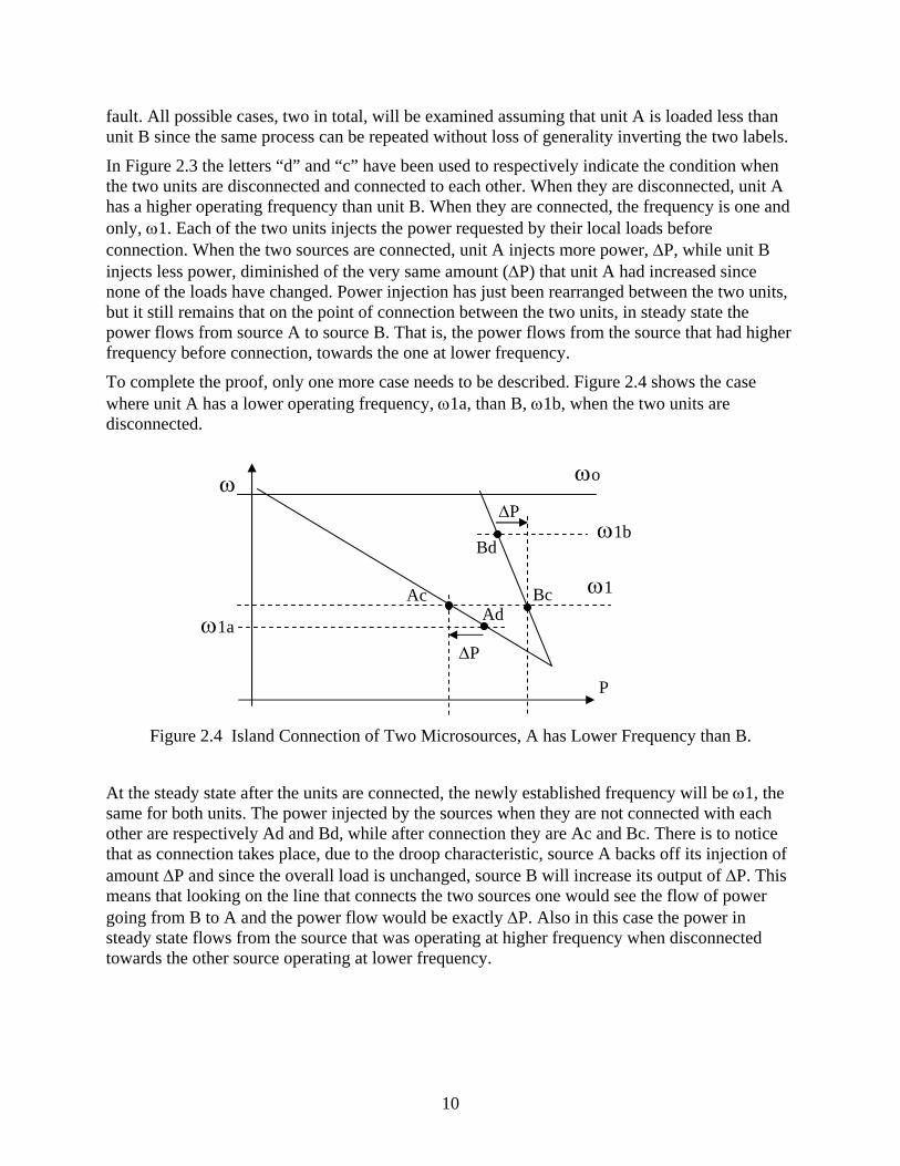
To complete the proof, only one more case needs to be described. Figure 2.4 shows the case where unit A has a lower operating frequency, ω1a, than B, ω1b, when the two units are disconnected.

Figure 2.4 Island Connection of Two Microsources, A has Lower Frequency than B.

At the steady state after the units are connected, the newly established frequency will be ω1, the same for both units. The power injected by the sources when they are not connected with each other are respectively Ad and Bd, while after connection they are Ac and Bc. There is to notice that as connection takes place, due to the droop characteristic, source A backs off its injection of amount ΔP and since the overall load is unchanged, source B will increase its output of ΔP. This means that looking on the line that connects the two sources one would see the flow of power going from B to A and the power flow would be exactly ΔP. Also in this case the power in steady state flows from the source that was operating at higher frequency when disconnected towards the other source operating at lower frequency.

ω1

ω ωo

ΔP

ΔP

Ad Ac

Bd

Bc

ω1a

ω1b

P

11

2.3 Synchronization Conditions The grid voltage E rotates at 60 Hz in the counter clockwise direction, while the microgrid voltage V rotates at a frequency lower than 60 Hz in the same direction. This means that if the vectors are strobed 60 times a second, the vector E stays motionless, while vector V recedes in the clockwise direction.

Figure 2.5 Receding Trajectory of Voltage Vector V.

Figure 2.5 shows the vector V rotating slower than E, so at each strobing it loses some angle from E. As time increases, V goes from position 1 to 4. The magnitude of the current resulting when the switch is closed is proportional to the voltage across the switch as the contacts are closed. The voltage across the switch is given by the vectorial difference between E and V. Near position 2 there is the maximum voltage across the switch and it would be a big mistake to close there because large transients in the current will ensue. Position 3 is better, but position 4 is where it is safe to close the switch.

Figure 2.6 shows the behavior in time domain: the difference in frequency has been artificially increased to make the point. In the upper plot, the solid line is the voltage of the grid, E, while the slower voltage, V, with longer period, is dotted. In the lower plot there is the voltage across the static switch. The best time to close the static switch is when the voltage across the switch is very small and contemporarily, the voltage of the grid is leading the voltage of the microsource. Therefore, anytime between time scale values of 30 to 35 is a good time to synchronize to the grid and close the switch.

E

V(1)

V(2)

V(3)

V(4)

12

Figure 2.6 Voltages on Either Side and Across the Static Switch.

When connecting two units together in island mode, each of the units is rotating at its own frequency, possibly none of them at 60Hz. The considerations made so far can be applied to a contactor that is responsible to connect the two units as long as the grid voltage is replaced with the voltage of the source that rotates faster and the microgrid voltage with the voltage of the source that rotates slower. It is possible to review the synchronizing conditions and express them in general terms that can be applied either to a static switch or to a contactor. The conditions that need to be contemporarily satisfied are:

i) the voltage across the switch must be very small

ii) the fastest rotating voltage must be leading the voltage that rotates slower

Condition (i) seems to be self-explanatory: closing with high voltage across the switch would determine an intolerable transient current. Voltage ratings are also at stake: if closing when the position of the voltage is at 2 in Figure 2.5, the initial condition for the current would be dictated by a voltage drop twice the nominal voltage of the system.

Condition (ii) may need some justification. The droop characteristic always determines a power flow from the unit operating at higher frequency to the lower frequency. This implies that when connecting to the grid, power is taken from the grid in steady state. When closing with the voltages across the switch determining a current of the opposite side, the current will grow at first then diminish and have a zero magnitude for a short time and then grow again, in the opposite direction. The power system can be described by differential equations: closing the switch with a certain voltage across it and with sources in the system applies an initial condition to a forced system. The voltage across the switch determines the initial condition, while the permanent, forcing terms are provided by the sources that follow the power versus frequency

13

droop. The issue is that it is possible to create an initial condition with a current that grows in the opposite direction from the forced solution that exists in steady state. The current must have only one transient: growing from zero to the final steady state value.

To make a stronger point, some simulation results with a single microsource connected to the grid will be shown. At first, the simulation will not meet condition (ii). Figure 2.7 shows the currents flowing in the static switch while Figure 2.8 shows the voltage across the static switch on the upper plot and the current injected by the microsource on the lower plot. Figure 2.9 shows the active power injected by the unit on the upper plot and the frequency of the microgrid on the lower plot. From all these plots it should be noticed:

a) the current from the grid increasing, going to zero (reversing) and then increasing again on all three phases

b) the microsource injects even more power than it is injecting in island, to feed the grid, and backs off immediately to the requested level.

c) the load always takes the same amount of power since its voltage is unperturbed, so the extra power that the microsource generates transiently goes into the grid.

The microsource power command is 0.2 pu, while the load takes 0.65 pu (all provided by the unit during island mode): transiently the source generates up to 0.9 pu, with the extra power being injected in the grid.

Figure 2.7 Three Phase Currents of the Static Switch, with Condition (ii) not Met.

Igrid_a [A]

Igrid_b [A]

Igrid_c [A]

Time [s]

14

Figure 2.8 Switch Voltage and Microsource Current, with Condition (ii) not Met.

Figure 2.9 Microsource Power Injection and Frequency, with Condition (ii) Not Met.

V_switch [V]

I_MS_a

Time [s]

P_MS [pu]

Frequency [Hz]

Time [s]

15

This synchronizing behavior is unacceptable because:

1) When the current reverses, also the flux in the magnetic cores of the transformers will change sign, creating a magnetoelectro-dynamic stress on the coils and it is reasonable to assume that every inversion transient will lower the life of the equipment.

2) Due to the fact that the output power of the microsource overshoots, it is impossible to synchronize when the unit operates near its rated power (say 90%) since this overshoot would bring the operating point beyond the rating of the source and as a result of this the equipment will trip.

It is time to look at a simulation when the switch is closed when the condition (ii) is verified. Figure 2.10 shows the vector plane with the voltage E and V. Remember that each of the voltages rotates counter clockwise, E at 60Hz and V at a frequency slightly lower. When strobing 60 times a second the vector E is still, while V recedes clockwise. As time increases, the voltage V goes from position 1 to 4. At this very point condition (i) for synchronization is verified, but it is position 5 that contemporarily verifies condition (i) and (ii) to achieve a safe synchronization to the grid.

Figure 2.10 Voltage Vector Plane Showing Correct Reclose Timing.

Figure 2.11 shows the three phase currents at the static switch as the synchronization takes place and the switch closes. There is still some transient due to the fact that the closing takes place on an R-L cable, but the current does not go through the reversal of direction.

E

V(1)

V(2)

V(3)

V(4) V(5)

16

Figure 2.11 Three Phase Currents of the Static Switch, with Condition (ii) Met.

Figure 2.12 Switch Voltage and Microsource Current, with Condition (ii) Met.

Igrid_a [A]

Igrid_b [A]

Igrid_c [A]

Time [s]

Time [s]

V_switch [V]

I_MS_a [A]

17

Figure 2.12 shows on the upper plot the voltage across the switch: the envelope of the voltage needs to go past the instant when it reaches the minimum value and then synchronization can take place. The lower plot of Figure 2.12 shows the current in the microsource, notice also the transient due to reclosing on an inductive network. The current drops to the lower value without any overshoot. The upper plot of Figure 2.13 shows the power of the microsource going from the full amount required by the load is island mode, 0.65 pu, to the value requested, 0.2 pu, never exceeding the value that it had during island mode. The lower plot of the same figure shows the frequency being locked to the grid value of 60Hz without first sagging towards an even smaller value, as seen in the previous simulation, Figure 2.9

Figure 2.13 Microsource Power Injection and Frequency, with Condition (ii) Met.

As already described, the synchronizing algorithm applies to the static switch that connects to the grid as well to the contactor that connects the two microsources together. To see that it is true, in the previous analysis one only needs to replace the grid voltage with the voltage of the unit that has the highest frequency. Indeed, it does not matter what is the operating frequency: all it matters is that the two voltages are rotating at different speeds. As of today, the hardware configuration of the static switch includes a logic block that enforcers condition (i) but not condition (ii).

The current hardware configuration correctly implements the first condition, but does not implement the second. Figure 2.14 shows the voltage across the switch during synchronization. The voltage diminishes in time due to the fact that the voltages at either ends of the switch rotate at slightly different frequencies. As soon as the voltage has reached a minimum threshold the synchronization takes place.

P_MS [pu]

Frequency [Hz]

Time [s]

18

Figure 2.14 Voltage Across the Static Switch During Synchronization, 1sec/div, 200V/div.

Figure 2.15 shows the current from the grid (upper plot) and the microsource (lower plot) when a single unit is connected to the utility. Before synchronization the current from the grid is zero because the static switch is open. As soon as it closes, due to the fact that the second condition is not implemented, the current starts flowing into the grid to immediately reverse after going through a cycle with zero magnitude. The microsource provides the extra transient current that is injected into the grid and then settles down to a lower value, since the utility is supplementing part of the quota of the load power demand.

Figure 2.15 Grid and Microsource Current During Synchronization, 100ms/div, 10A/div.

19

Chapter 3. Microsource Details

This chapter gives the details of the system that composes a microsource. Figure 3.1 shows the microsource layout implementation. The controller sends the gate pulses to the inverter that generates a three phase 480V line to line voltage. This waveform is rich in harmonic content at the switching frequency, 4kHz. To filter out these harmonics there is a low pass LC filter immediately connected at the inverter terminals. Then there is the series of the coupling inductance and transformer. The sensed quantities are the voltages at the load bus and the inverter currents. From these quantities it is possible to extract the load voltage magnitude and the active and reactive power injected by the unit. If the unit controls the feeder power flow, then the measures of the currents flowing on the feeder from the side that connects to the grid are also passed to the controller to enable the calculation of this active power flow.

Figure 3.1 Microsource Diagram.

3.1 Microsource Controller This section gives the details of the final form that the control assumes during the implementation. Hardware realization of the control has been plagued by issues of noise propagation from the analog to the digital word inside the controller. The fundamental frequency selective filter is a first tool to handle some of the higher harmonics of the noise, but the calculated values of active and reactive power, as well as the voltage magnitude still suffered from oscillations determined by random spikes in the measured quantities.

The complete control of the microsource is shown in Figure 3.2 [4]. The inputs are either measurements (like the voltages and currents) or setpoints (for voltage, power and the nominal grid frequency). The outputs are the gate pulses that dictate when and for how long the power electronic devices are going to conduct. The inverter voltage and current along with the load voltage are measured. The voltage magnitude at the load bus and the active power injected are then calculated. When controlling active power, there is a choice of regulating the power coming from the unit or the power flowing in the feeder where the source is connected. If the power in

FX

FC

)t(vabc

+

VDC Inverter

Controller

LocalFeeder

Gate Signals

X

)t(i)t(e

abc

abc

480 V 208 V

n

Towards Grid

Feeder Currents )(tiabc

FX

20

the feeder is regulated then there is a need to bring in the measure of the current flowing in that branch.

The voltage is calculated from the stationary frame components of the filtered instantaneous voltages. The desired and measured values for the voltages are then passed to a dynamic block that implements the P-I response of the voltage control. The output is the desired voltage magnitude to be implemented by the gate pulse generator block. This version includes low pass filters on the P, Q, and V calculated quantities to reduce the propagation of the effects of noise. These filters have also a secondary desirable effect: they attenuate the magnitude of the 120Hz ripple that exists during unbalanced operation. This allows the control to survive conditions of load unbalance without having to take any corrective action.

This final version of the control focuses on the configuration that regulates the power injected by the unit. This is not a loss of generality, since to implement the load tracking configuration one needs just two modifications: the first is to introduce the measure of the line current to calculate feeder flow, still retaining the inverter current measure to calculate the reactive power injected by the unit. The second modification is to invert the sign of the droop coefficient of the power-frequency characteristic to take into consideration that now it is the line power that is regulated and not the power injected by the unit.

Figure 3.2 Final Version of Microsource Control.

One of the main objectives for the control is portability when adopted in units of different nominal ratings. To satisfy this requirement, the control has been designed so that all the internal quantities are in a per unit system. This implies that whether the size of the unit is 30kW or 200kW, the power is internally represented always as a quantity that is between zero and unity values. The same considerations are applied to the voltage rating of the feeder where the units are installed. Rescaling quantities in a per unit system implies that the PI gains and the droop coefficients do not need to be calculated again each time one decides to use this control on a unit

Inverter Current

cbainvi ,,

Inverter or Line Current

Magnitude Calculation

Voltage Control

Q Calculation

Q versus E Droop

P Calculation

P versus Frequency Droop

Load Voltage Measure

Q

P

oP

oE

Vδ

reqE

Gate Pulse Generator

to Inverter

Gates

oω

E V

Low-Pass Filter

Low-Pass Filter

Low-Pass Filter

21

with different size. This control is somewhat universal because of its ability to be used with different hardware configurations without having to change anything internally. Every block will be expanded to show the operations on the variables inside.

The active power is regulated to a desired value during operation in parallel with the grid. During transfer to island operation, the frequency of the network will be allowed to sag slightly, adopting the active power-frequency droop. The characteristic will ensure that all the units will immediately ramp up their output power to match the missing quota from the grid, without the usage of an explicit network of communication between the several units. This P versus frequency block generates the angle that will be tracked by the gate pulse generator.

Each of the blocks that appear in Figure 3.2 will be examined in detail: the only block that it is left out is the gate pulse generator, that will be described in great detail in Section 6.4.

3.1.1 P and Q Calculation The blocks that calculate the values of active and reactive power will use the knowledge of instantaneous values of line to line voltages and line currents. These are exactly the quantities that are brought in from the sensing equipment. Since there is no ground to refer to, the voltages are always measured across the phases. The count of the sensing equipment is kept to a minimum by measuring only two of the line to line voltages and calculating the third one from the fact that the sum of the three delta voltages must equal zero, in balanced as well under unbalanced conditions. Only two currents are measured and the third one is calculated assuming their overall sum to be zero, which is correct only under balanced conditions.

Figure 3.3 P and Q Calculation Blocks.

Figure 3.3 shows the input-output layout for the P and Q calculation. Notice that the measure of the voltage at the microgrid side is passed to both blocks, while the current can either be the inverter current or the feeder current, depending respectively if the output power of the microsource or the power flow on the feeder is controlled.

The equations used are:

Inverter Current

cbainvi ,,

Inverter or Line Current cbai ,,

Q Calculation

P Calculation

Load Voltage Measure ,, cbae

Q

P

P and Q calculation

22

( ) ( )3

ii2eii2eQ

ieieP

abcababc

aabcbc

+++−=

−=

One advantage of adopting these equations is that they use quantities that are readily available, namely the line to line voltage measure that does not need to be converted to line to neutral. Another advantage is the simplicity of the equations that do not require the extra step of being converted to rotating frame components, since the powers are evaluated from the immediately available time domain quantities obtained from the sensing equipment.

3.1.2 Voltage Magnitude Calculation The block of Figure 3.2 labeled Magnitude Calculation is expanded in Figure 3.4. It uses information on the time domain line to line voltage to calculate the magnitude for the load side voltage.

Figure 3.4 Voltage Magnitude Calculation Block.

The selective filtering of the voltage components has the desirable effect of removing the high frequency random noise components that inevitably creep in the real world of sensing equipment. The overall output of this block is the magnitude of the voltage.

The selective filter, shown in Figure 3.5 is achieved with two integrators that implement an oscillator, removing any component that is not at the specified frequency [5]. This frequency is obviously chosen to be the system nominal frequency. This selective filtering has two possible outputs: Pu is the output in phase with the input signal, u, while Qu is the output that is behind, in quadrature with respect to the input signal.

d-q Stationary Frame

Transformation

Cartesian To

Polar

ae

be

ce

qe

de

Magnitude Calculation

E Selective

Filter

Pae Pbe Pce

23

Figure 3.5 Selective Filter Diagram.

Figure 3.6 shows the magnitude and phase response of the filter. The magnitude shows that the frequency 60Hz is passed without any alteration, i.e. unitary gain (zero dB) and zero phase shift. For frequencies very near to 60Hz the gain is a little lower than one and phase shift is non-zero. That is not a problem: by choosing an appropriate value for KF, it is possible to ensure that the gain is lowered only of a fraction of a percent for the range of frequencies expected during island operation. The phase shift is also not a problem: since all components are shifted of the same amount, the shift can assume any arbitrary value. The calculation of P and Q is a function of the relative shift of voltages and currents, not their absolute value. As long as both voltages and currents are shifted of the same amount (and they are, since the frequency of voltages and currents are the same), then their relative phasing will remain unaltered.

Figure 3.6 Selective Filter Response.

o

FKω

s

oω

soω

u

+

_

_

+ Pu

Qu

24

The ‘d-q’ axis components are found by projecting the rotating phase voltages over a fixed reference frame with two axis in quadrature. The equations are:

))(

21)(

21)((

32)(

3)()()(

tetetete

tetete

cbaqs

bcds

−−⎟⎠⎞

⎜⎝⎛=

−=

Eq. 3.1

These components are then converted to magnitude and phase by a change of coordinates, from Cartesian to Polar:

22qd eeE += Eq. 3.2

3.1.3 Voltage Control The Voltage Control block is shown in detail in Figure 3.7. The output of this block interfaces with the inverter that implements the space vector technique synthesizing directly this desired voltage magnitude. The inputs of this block are the requested value adjusted from the Q-voltage droop and the measure of the magnitude of the voltage at the feeder bus. This block is the core of the voltage control: the voltage at the load is regulated by creating an appropriate voltage at the inverter terminals.

Figure 3.7 Voltage Control Block.

This block compares the measured and the desired voltage magnitudes. This error is passed inside a P-I controller to generate the desired voltage magnitude at the inverter.

3.1.4 Q versus E Droop Figure 3.8 shows the details of the operations taking place inside the block called “Q versus E droop” in Figure 3.2. This block implements the reactive power versus voltage droop, its main action is to adjust the externally requested value of voltage to a value that will require less injection of reactive power to be tracked.

P-I

oE

+_

Voltage Control

E V

25

Figure 3.8 Q versus Load Voltage, E, Droop Block.

The inputs of this block are the desired voltage at the regulated bus and the current injection of reactive power from the microsource. The output is the new value of voltage request that replaces the one commanded from outside. This new value is obtained from the linear characteristic of the droop.

Figure 3.8 expands the block labeled as “Q versus E droop” in Figure 3.2 to allow to see the details. This block is responsible for modifying the value of the reference voltage that is commanded from outside. When two units are located electrically near each other and given two voltage setpoints, they will try to achieve those requested voltages by injecting reactive power. If the two setpoints are somewhat different from each other, then one machine will inject a large amount of capacitive power, while the other will inject inductive power.

This situation comes as a consequence that the units will have to create the requested difference of voltage by injecting a large current over the small impedance that there is between the units. In this scenario reactive current will flow from one unit to the other, creating the problem of the circulating currents. These currents flow in the machines, reducing the amount of ratings available to face new load requests.

To mitigate this problem, a reactive power versus voltage droop is adopted. This characteristic is designed to convert the external command of the voltage reqE into the value oE . The larger is the amount of capacitive power that is injected, the lower this value is allowed to sag compared to the external request. Conversely, oE is allowed to swell as inductive current is injected. In this way, if two neighboring units have voltage setpoints reqE that are too far apart, then the actual commands oE of the units will result nearer to each other. This correction successfully limits the circulating reactive currents because it limits the reactive power injections to achieve the adjusted voltages. The characteristic is represented in Figure 3.9 where it is possible to see how the block corrects the reference voltage according to the sign of the injected reactive power.

Qm Q

reqE

oE _

+

Q versus E Droop

26

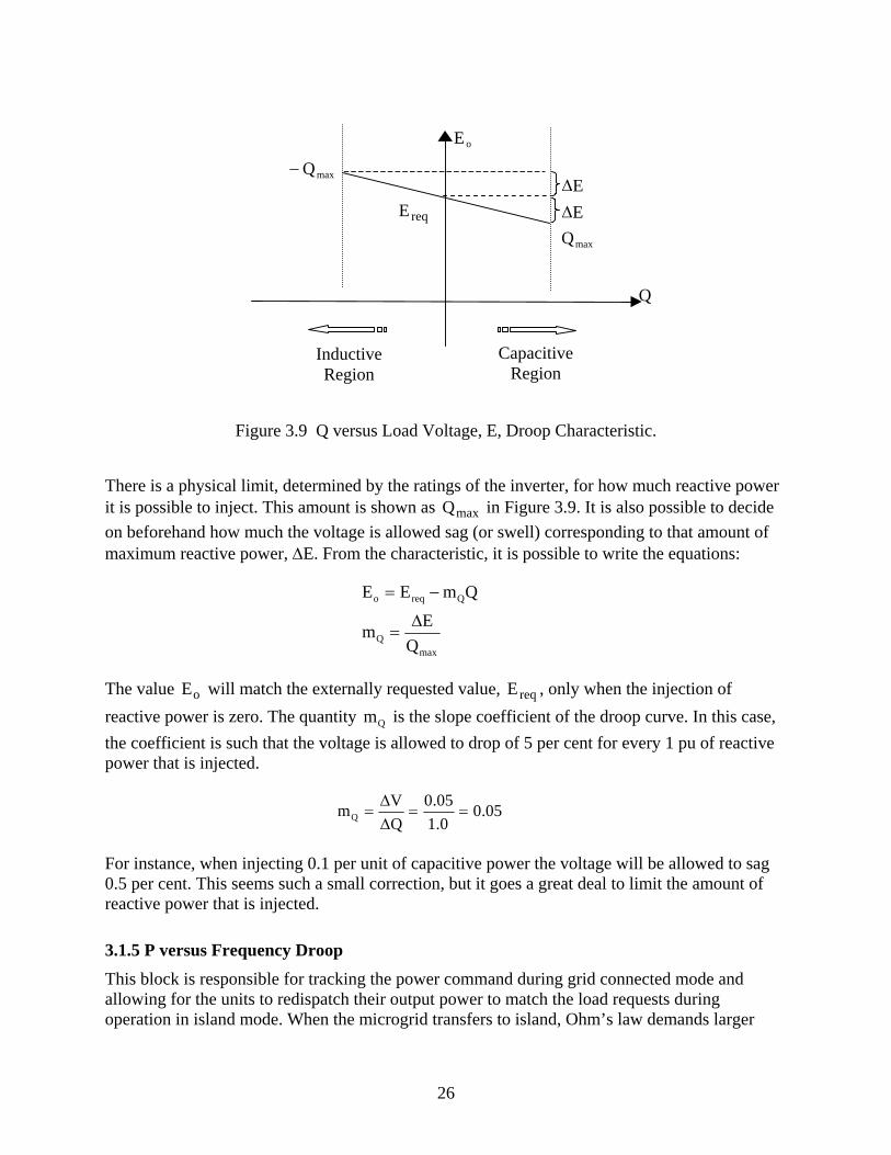
Figure 3.9 Q versus Load Voltage, E, Droop Characteristic.

There is a physical limit, determined by the ratings of the inverter, for how much reactive power it is possible to inject. This amount is shown as maxQ in Figure 3.9. It is also possible to decide on beforehand how much the voltage is allowed sag (or swell) corresponding to that amount of maximum reactive power, ΔE. From the characteristic, it is possible to write the equations:

maxQ

Qreqo

QEm

QmEE

Δ=

−=

The value oE will match the externally requested value, reqE , only when the injection of reactive power is zero. The quantity Qm is the slope coefficient of the droop curve. In this case, the coefficient is such that the voltage is allowed to drop of 5 per cent for every 1 pu of reactive power that is injected.

05.00.105.0

QVmQ ==

ΔΔ

=

For instance, when injecting 0.1 per unit of capacitive power the voltage will be allowed to sag 0.5 per cent. This seems such a small correction, but it goes a great deal to limit the amount of reactive power that is injected.

3.1.5 P versus Frequency Droop

This block is responsible for tracking the power command during grid connected mode and allowing for the units to redispatch their output power to match the load requests during operation in island mode. When the microgrid transfers to island, Ohm’s law demands larger

EΔ

EΔ

oE

Q

maxQ

max Q −

InductiveRegion

CapacitiveRegion

reqE

27

currents from the microsources increasing their measure of output power, and as a consequence of the droop the units will operate at a frequency slightly smaller that nominal system value.

Figure 3.10 Power – Frequency Droop Characteristic.

Figure 3.10 shows the characteristic of the power versus frequency droop. Two units, a and b are shown here: their power setpoint when connected to the grid are respectively Pao and Pbo. Both characteristics allow power to increase as the frequency decreases. During islanding the frequency sags to a new value, ω1, and the microsources respectively generate Pa1 and Pb1 power. Two things need to be pointed out: the difference of the sum of generation in island (Pa1+Pb1) and during grid connection (Pao+Pbo) is the missing quota of power from the grid. The second important point is that since the slopes of the droops are constant, the two units pick up power in the same amount, that is one ramps up of as much in per unit as the other does.

Figure 3.11 Block Diagram of the Active Power Droop.

The control block that realizes the droop is represented in Figure 3.11: there are only three inputs to the block: the desired and measured injected power and the nominal system frequency. The measure of the angle of the voltage at the regulated bus is not needed because that information is already implicitly fed back through the value of the measured power injected by the microsource. The output of this block is the desired angle of the voltage at the inverter bus: this is because the

P versus Frequency droop

m s1

vδ +

_ _

+

oP

P ωΔ

oω

π+

π−

ω

Unit a Unit b

P

ω

oω

1ω

aoP

boP

1aP

1bP

28

gate pulse generator based on the space vector synthesizes directly the angle of the desired voltage.

The droop characteristic is realized by multiplying the coefficient ‘m’ with the error for power. The droop coefficient ‘m’ represents the slope of the characteristic, and it depends on the values of Pmax, ωmin and current power setpoint. The expression for ‘m’ is:

max

min

Pm o ωω −

−=

The angle is obtained by integrating the instantaneous quantity ω wrapped around +π and –π. This is because the command req vδ is constantly increasing with rate at or near oω , so to avoid overflow of this variable inside the DSP register, the angle is reset to –π each time it reaches +π, therefore the quantity req vδ will look like a sawtooth.

3.2 Power Control Mode with Limits on Unit Power

This section gives a general view of the issue of limits in distributed generation. Each unit is composed of a prime mover, an energy storage device and an inverter that interfaces with the system as shown in Figure 3.12

Figure 3.12 Microsource Elements: Prime Mover, Storage, Inverter.

The problem of reaching maximum output power needs to be addressed to avoid that the energy storage is either depleted or filled up over capacity. The prime mover does not have a problem exceeding the maximum power because it simply cannot do it. The maximum power exists because of the fact that the prime mover is not able to generate more power than that. The inverter ratings are slightly larger than this maximum active power limit because of the need to provide reactive power as well as active power at the same time. Reactive power injection is required to perform voltage regulation.

As soon as the load conditions (P and Q combined) determine an overall output that is above the ratings of the inverter, then protections will ensure survival of the silicon devices by tripping the unit off.

The basic difference between limits in the prime mover and limits in the inverter is that the prime mover cannot physically give more than its maximum power, so it would reach this limit and hold it. The inverter could inject more than its own power rating (nothing physical prevents it from doing it), so to prevent damage the protections would intervene. Reaching this kind of limit that requires intervention of protections has nothing to do with this section. Overshooting the

Prime Mover

(Gas Turbine, Fuel Cell, Internal Combustion Engine …)

Energy Storage

(Ultracapacitor, Battery,

Flywheel…)

Inverter

DC Link Fuel 0 < P < Pmax

P, Q to 3-phase AC

System

29

inverter ratings limits (in kVA) can only result in shutdown and is the topic of protection analysis.

This report is about preventing the inverter from injecting a steady state output power that is larger than maximum prime mover output. If that were to occur, the storage would deplete all its energy. This suggests that as long as the inverter is within its apparent power ratings (kVA) it is possible to overshoot the maximum power limit (kW) without compromising equipment safety. Some action must be taken to avoid that this overshoot is sustained in steady state, by enforcing the behavior of the unit to belong to some particular characteristic.

This report is also about preventing the inverter from injecting a steady state output power with a negative sign: if that were to occur, the storage would overshoot its maximum capacity. This limit is defined by the fact that the prime mover cannot behave like a load. For instance, microturbines are thermodynamic machines that convert chemical energy of the fuel into mechanical power. This machine will not be able to perform the opposite task of using mechanical power to convert it to some other form. It follows that the prime mover has the value of P = 0kW as the lower limit of power. The inverter does not have such an issue. It can legally operate in all four quadrants of the P,Q plane as long as its ratings are not exceeded. In practice, the voltage and current flowing in the inverter could have a phase displacement so that the overall active power injection is negative. This power cannot be transferred to the prime mover, an would be stored in the battery. A steady state operation in this condition would overfill the energy storage. To avoid this situation there is the need to prevent the inverter from ever exceeding minimum power during steady state, acknowledging the fact that it would be legal to overshoot this limit for a short period of time.

3.2.1 Steady State Characteristics with Output Power Control This section describes the configuration with the control regulating the voltage and the power injected by the unit at the local point of connection with the feeder to a desired amount. To this end, the active power injected and the feeder voltage are measured and passed back to the control loop. Figure 3.13 shows the diagram of this configuration: the measure of power injected by the unit, P, is calculated from the current injected by the source and the voltage E measured at the point where the unit is installed.

This chapter shows the steady state characteristics on the power vs. frequency plane that allow to enforce limits for the output active power and frequency. This chapter describes the characteristics to be used when the units are configured to regulate their output active power. Figure 3.13 shows that when connected to the grid, load changes are matched by a corresponding power injection from the utility. This is because the unit holds its injection constant. During island mode all the units participate in matching the power demand as loads change.

30

Figure 3.13 Diagram of a Unit Regulating Output Active Power.

In this case there is no mean of controlling the power that comes from the grid: it can indirectly be changed by choosing different setpoints for the power of the unit, but the amount of power that is drawn from the AC system cannot be planned ahead. With this system of regulating active power, it is impossible to sign a contract with the utility agreeing on a determined amount of power to be taken: the units can only control their power output, without any notion of the power from the grid. The amount of power dispatched by the units when the grid is connected is arbitrary and dependent on the choices of the managers of the units inside the microgrid.

This configuration can take full advantage of the Combined Heat and Power (CHP) applications, where total (electric+heat) system efficiency is maximized when the waste heat from power production is also used. In this way, electricity production is only requested when there is also heat load demand resulting in great levels of total efficiency.

The system can operate in island mode because of the power-frequency droop that allows the units to share the extra power demand. The minimum requirement for every microsource is to regulate power and voltage to desired values when connected to the grid. During island mode, the power must automatically and independently readjust in every machine so that the new level of power output matches the demand from all sensitive loads present in the microgrid.

The voltage is regulated at the bus where the source is connected to the feeder belonging to the microgrid. Figure 3.14 shows the unit power configuration, where the source directly regulates the power injected by the unit.

When all the sources have their own power commands set, any load change taking place within the microgrid will be matched by a corresponding amount of power imported from the utility. This mode of operation is the most traditional because it follows directly from the operation of any existing power plant.

X Rest of the System

Loads

Micro-Source

sourceP

E

E, I I

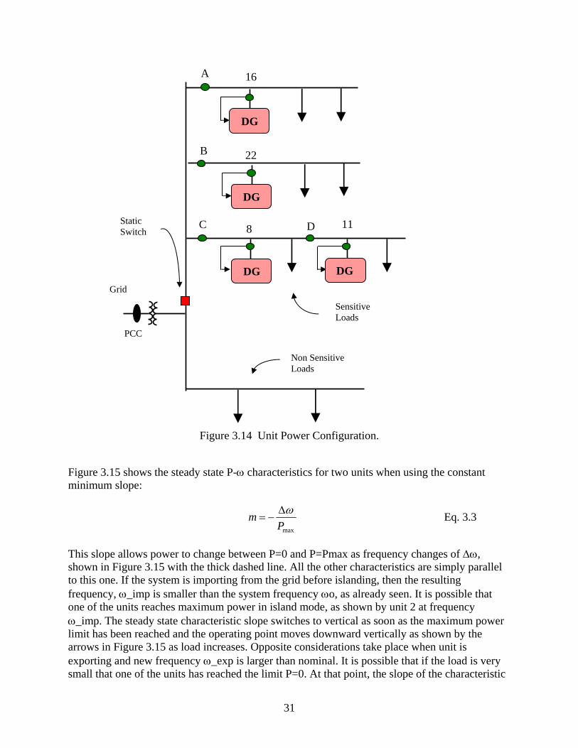
31

Figure 3.14 Unit Power Configuration.

Figure 3.15 shows the steady state P-ω characteristics for two units when using the constant minimum slope:

maxP

m ωΔ−= Eq. 3.3

This slope allows power to change between P=0 and P=Pmax as frequency changes of Δω, shown in Figure 3.15 with the thick dashed line. All the other characteristics are simply parallel to this one. If the system is importing from the grid before islanding, then the resulting frequency, ω_imp is smaller than the system frequency ωo, as already seen. It is possible that one of the units reaches maximum power in island mode, as shown by unit 2 at frequency ω_imp. The steady state characteristic slope switches to vertical as soon as the maximum power limit has been reached and the operating point moves downward vertically as shown by the arrows in Figure 3.15 as load increases. Opposite considerations take place when unit is exporting and new frequency ω_exp is larger than nominal. It is possible that if the load is very small that one of the units has reached the limit P=0. At that point, the slope of the characteristic

Grid

Sensitive Loads

Non Sensitive Loads

Static Switch

DG DG

DG

DG

16

22

8 11

PCC

A

B

C D

32

is switched to vertical and as load decreases, the operating point moves upwards, as shown by the arrows in Figure 3.15.

The minimum and maximum power limits are enforced by the fact that the characteristic with constant slope are switched to a vertical steady state characteristics.

The minimum and maximum frequency limits cannot be overshoot because it would imply, respectively, that the loads have exceeded the overall generation capability or that the load is actually injecting power into the system. These last two limits do not need to be explicitly enforced since the assumption on the load (smaller than sum of all generation, but never smaller than zero) automatically implies behavior within frequency limits.

Figure 3.15 Steady State P-ω Characteristics with Fixed, Minimum Slope.

This approach has the advantage of being able to enforce both limits in power and frequency while adopting a fixed value for the slope. Only power limits need to be enforced, frequency limits come as a consequence.

The fundamental idea is that the control needs to be augmented with some blocks responsible to enforce limits. To prevent changing the system behavior as we know it, these blocks shall be inactive at any time the unit is not exceeding the limits. Figure 3.16 allows to understand what these added blocks need to change and how.

ω

Δω

Δω

oω

P

1oP 2oP Exporting

to Grid

Importing from Grid impω

expω

Pmax

33

Figure 3.16 Effectively Limiting Pmax on Output Power Control.

Figure 3.16 shows two units in island mode operating at the frequency ω1 (circles) where unit 2 has:

P1(at ω1) = P1_1

P2(at ω1) = Pmax + ΔPmax

Here, ΔPmax is the amount of power that is given in excess of Pmax. The main idea is that a change must be performed so that at the final operating point unit 2 is injecting Pmax (and no more), while unit 1 injects the amount of power that it had previously added of the excess of power (ΔPmax ) of unit 1:

P1(at ω2) = P1_1 + ΔPmax

P2(at ω2) = Pmax

Frequency ω2 is also shown on Figure 3.16 and the corresponding power outputs are shown with squares. Notice that the sum of power injected does not (and must not) change between the two frequencies, since the overall sum of the load demand has not changed. The question now is how to make sure that unit 1 (that reaches max) will rearrange its frequency as to end up at frequency ω2 and not ω1. The reason why it would reach ω1 in the first place is because of the droop equation, reported here for convenience:

( )iiooi PPm −−= ,ωω Eq. 3.4

Pmax P = 0 Output Power Within Limits

P

ω

ΔPmax

ΔPmax Unit 1

Unit 2

Unit 2 Max

oω

1ω

2ω Δωmax

34

The only way to make sure that the frequency would be readjusted is to add a term to this equation and modify it as follows:

( ) max, ωωω Δ+−−= iiooi PPm Eq. 3.5

If Δωmax = 0 when the output power is within limits then Eq.3.5 is effectively identical to Eq. 3.4. And if Δωmax is calculated so that it generates an appropriate amount of frequency change (in this example Δωmax= ω2-ω1, negative value), when limits are exceeded, then max power can be enforced. Eq. 3.4 is represented in Figure 3.16 by the “Unit 2” characteristic, while Eq. 3.5 is represented by the “Unit 2 Max” characteristic. This second characteristic is obtained from the first by adding a frequency offset Δωmax that translates down on the P-ω plane the original characteristic. Notice that since unit 1 does not reach maximum, then its offset will be calculated as zero and the original characteristic (Eq.3.4) is enforced at all times. Next section gives the details on how to generate this appropriate value of frequency offset to achieve maximum power limiting.

Now the attention is to find the changes that need to be done when zero power limit is exceeded. It will be shown that this problem is the mirror image of the max power problem. Figure 3.17 shows the units operating in island at the frequency ω1, circles, with unit 1 injecting negative power. The output power of the units at this frequency is:

P1(at ω1) = Pmin – Δpmin (Pmin = 0)

P2(at ω1) = P2_1

ΔPmin is the excess power over the minimum limit that unit 1 is injecting. The ideal solution would be to operate at the frequency ω2, squares, where unit 1 is held at the zero power level while unit 2 injects the power it had before minus the amount of power that unit 1 is no longer adsorbing (ΔPmin). The output from the units at this new frequency are:

P1(at ω2) = Pmin (Pmin = 0)

P2(at ω2) = P2_1 - Δpmin

Notice that the sum of the power injections is the same at either frequencies because the sum of all the loads has been assumed constant.

The problem is that at frequency ω2, unit 1 is operating at a point that does not belong to the characteristic labeled “Unit 1”, but rather to the characteristic labeled “Unit 1 Min”. Respectively, the first one is generated by Eq. 3.4, while the second one is generated by the following equation:

( ) min, ωωω Δ+−−= iiooi PPm Eq. 3.6

35

Figure 3.17 Effectively Limiting Pmin=0 on Output Power Control.

Where in this case Δωmin=(ω2-ω1), positive number, in steady state. Δωmin=0 each time the power output is larger than zero to ensure that the behavior of the unit follows the desired characteristic of Eq. 3.4. Notice that Δωmin translates upwards the original characteristic enforced when no limit is exceeded. Next paragraphs deal on how to generate the offsets for maximum and minimum power excursions.

It is possible to take advantage of two assumptions:

1) the prime mover will never give a fraction of extra power over P_max, but because of the storage interface, there is some extra power available transiently. Furthermore, the inverter is rated to be able to inject over P_max as stated in Section 3.4. Therefore it is assumed that there is enough stored energy available and silicon ratings to deliver it so that the inverter can transiently sustain overshoots of the value P_max for short periods of time.

2) as soon as the inverter is absorbing power, (P<0), the power electronic devices behave like a bridge of diodes due to the reversed current polarity. Energy is transferred from the feeder to the DC storage. It is assumed that the storage device can transiently sustain the condition of P < 0 for brief periods of time.

When preventing injections of power exceeding maximum value, the first step to obtain the frequency offset is to generate a power error with the reference set to Pmax, and obtain the quantity errP_max as shown in Figure 3.18.

Pmax P = Output Power Within Limits

P

ω

ΔPmin

ΔPmin

Unit 1

Unit 2

Unit 1 Min

oω

1ω

2ω

Δωmin

36

Figure 3.18 Offset Generation to Limit Max Power with Integral Block.

This error is passed it to an integral block that has a dynamic limiter which prevents its output to ever become positive. This limiter makes this integral path non-linear. The integral can always integrate up and down (depending on the sign of errP_max) but its output will be truncated to zero and never allowed to become positive. With this approach, Δω_max is either a zero or a negative quantity only.

As long as power is lower than max, errP_max is positive and the output of the integral is dynamically limited to zero, correctly generating a zero offset when the unit is operating below Pmax.

If power is larger than maximum, errP_max is negative and the integral would start generating a negative value for the offset. This offset in turns translates the characteristic down (see Figure 3.16). It will keep on translating down up until the offset exactly matches the value for which errP_max = 0. As long as it is not, the integral would keep on increasing the offset. When power output matches maximum power the error would become zero and the integral would stop increasing the offset: a new steady state has been reached at the frequency ω2 (Figure 3.16) with offset Δωmax = ω2-ω1.

This control proved to be effective to limit power, but the analysis would not be complete without showing that the process of reaching a maximum is reversible. To understand this concept, consider the following series of states and actions:

i) Steady State: units within limits,

ii) Action: load increase

iii) Steady State: a limit is reached is held

iv) Action : load decrease

v) Steady State: units within limits

The system is considered memoryless or reversible if the state (i) is identical to the state (v), that is, the system has no memory that it went through states (ii) through (iv).

To verify reversibility, consider the following: at first the system on state (i) operates on the characteristic “Unit 2” in Figure 3.16. After a load increase (that engages max power output regulation) the characteristic has been effectively changed from “Unit 2” to “Unit 2 Max”, represented by state (iii). When the load decreases (iv) then the unit would continue to operate on this second characteristic and power will become smaller than maximum. But as soon as this happens, the errP_max of Figure 3.18 becomes positive and the negative offset Δωmax becomes smaller and smaller. The dynamic limiter in the integral will prevent it from ever assuming a

maxP

maxerrP maxωΔ

+ s

Ki

0P

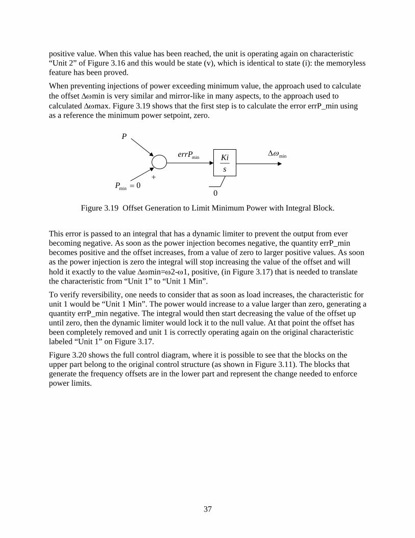
37

positive value. When this value has been reached, the unit is operating again on characteristic “Unit 2” of Figure 3.16 and this would be state (v), which is identical to state (i): the memoryless feature has been proved.

When preventing injections of power exceeding minimum value, the approach used to calculate the offset Δωmin is very similar and mirror-like in many aspects, to the approach used to calculated Δωmax. Figure 3.19 shows that the first step is to calculate the error errP_min using as a reference the minimum power setpoint, zero.

Figure 3.19 Offset Generation to Limit Minimum Power with Integral Block.

This error is passed to an integral that has a dynamic limiter to prevent the output from ever becoming negative. As soon as the power injection becomes negative, the quantity errP_min becomes positive and the offset increases, from a value of zero to larger positive values. As soon as the power injection is zero the integral will stop increasing the value of the offset and will hold it exactly to the value Δωmin=ω2-ω1, positive, (in Figure 3.17) that is needed to translate the characteristic from “Unit 1” to “Unit 1 Min”.

To verify reversibility, one needs to consider that as soon as load increases, the characteristic for unit 1 would be “Unit 1 Min”. The power would increase to a value larger than zero, generating a quantity errP_min negative. The integral would then start decreasing the value of the offset up until zero, then the dynamic limiter would lock it to the null value. At that point the offset has been completely removed and unit 1 is correctly operating again on the original characteristic labeled “Unit 1” on Figure 3.17.

Figure 3.20 shows the full control diagram, where it is possible to see that the blocks on the upper part belong to the original control structure (as shown in Figure 3.11). The blocks that generate the frequency offsets are in the lower part and represent the change needed to enforce power limits.

P

0min =P

minerrP minωΔ

+ s

Ki

0

38

Figure 3.20 Control Diagram to Enforce Limits with Unit Power Control.

The equation that governs this control has been formally changed from Eq. 3.4 to an equation that keeps into account of changes made in Eq. 3.5 and Eq. 3.6 when respectively dealing with maximum and minimum power limits. The final equation is:

( ) minmax, ωωωω Δ+Δ+−−= iiooi PPm Eq. 3.7

The quantities Δωmax and Δωmin are added to the frequency as calculated in Eq. 3.4. Both quantities are zero when the unit operates within power limits. When Pmax is exceeded, then Δωmax becomes negative (never positive) to enforce the limit. Conversely, when Pmin = 0 is exceeded, then Δωmin becomes positive (never negative) to enforce the limit.

This control has been implemented in simulation and hardware and the results obtained prove the effectiveness of the control design. The control is tested with all known events that can cause either limit to be exceeded: these hardware results are all included in Chapter 7.

3.2.2 Steady State Characteristics with Feeder Flow Control

Another possible option for controlling power is to regulate to a constant the flow of active power in the feeder where the unit is installed. The main reason why there is an interest in exploring the load tracking configuration is because when regulating power on the branches to a constant value, then the power supplied from the grid will remain unchanged when a load changes inside the microgrid. There are cases when the utility is interested in having large customers to draw a constant amount of power from the grid, regardless of their changing local

m

oω

+

s1

)(tVδ ω oP

P

+

_ +

maxωΔ

maxerrPmaxP

+

sKi

0

minerrP

0min =P

+

sKi

0

+

minωΔ

P

39

needs of power. This solution would solve this problem and the grid would see a constant power demand from the microgrid.

The basic requirement for the load dispatch configuration is the need for a measure of the power flowing in those branches so that the control can compare it against the desired reference amount. Figure 3.21 shows this configuration, where it is possible to see that the power from the line and the power from the unit always add up to the load request. When a load increases the unit increases its power output to maintain a constant branch power flow. This configuration implies feedback of the line current and the voltage at the point where the unit is installed to calculate the power flow in the feeder.

This section shows the steady state characteristics on the F-ω plane that allow to enforce limits on frequency and unit power output, P. In this case the units are configured to regulate the flow of power in the feeder that connects to the utility, F. Figure 3.21 shows the setup: when connected to the grid, every load change is matched by a different power injection from the unit since the control holds the flow of power coming from the grid, F_line, to a constant value. During island mode all the units participate in matching the power demand as loads change.

Figure 3.21 Diagram of a Unit Regulating Feeder Power Flow.

The case when the grid fails while operating in the load dispatch mode can be handled by changing the sign of the power-frequency droop characteristic. During island mode there is less need to import power from the feeders so that the characteristic is designed to reduce power as the frequency reduces.

Figure 3.22 shows the load tracking configuration for the whole microgrid. This mode of operation earned this name because once the required level of power requests are set, any change in load within the microgrid will be matched by a corresponding amount of power injected by the units to keep the flow in the feeder constant. This configuration has the advantage that the microgrid looks exactly like a dispatchable load from the utility point of view. New agreements in electric contracts can be signed with the utility: for instance the microgrid could agree to behave like a constant load during a determinate period of time of the day since it can automatically track all its internal changes of load with the local generation.

X Rest of the System

Loads

Micro-Source

sourceP

lineF

FeederI

E

FeederI ,E

40

This creates advantages on both sides of the meter: the utility is guaranteed a limit on the amount of power taken by a certain region where multiple microgrids are present, while due to this restriction on the power usage, microgrids could enjoy lowered electricity rates during those periods of times when the restriction applies.

Figure 3.22 Load Tracking Configuration.

The fact that the power on the feeder needs to be regulated implies that there is a need to install sensing equipment on that feeder to evaluate the power and feed it back to the microsource controller. In short, this implies an increase in the component count for the sensing equipment. The advantages that load tracking offer may be more than enough to offset the nuisance of having to install measuring equipment directly on the feeder of the microgrid floor, rather than having them nicely encased within the chassis of the microsource.

Figure 3.23 shows the characteristics of two units adopting the feeder power flow control. The characteristics enforce the following relation:

( )iioFoi FFm −−= ,ωω Eq. 3.8

Grid Sensitive Loads

Non Sensitive Loads

Static Switch

DG DG

DG

DG

16

22

8 11

PCC

A

B

C D

41

This expression is very similar to Eq. 3.4 used for unit output power control. The slope has fixed identical magnitude of the minimum slope of Eq. 3.3, but has a reversed sign ( mmF −= , the characteristics are slanted the opposite way). The sign needs to be reversed because of the relation between the output power, P and the feeder flow F. This relation can be derived by inspection of Figure 3.21:

Fi + Pi = Li for unit ‘i’ Eq. 3.9

Fi is the power (imported means positive) from the rest of the system

Pi is the power injected by the unit (subjected to belong to [0, Pmax] interval)

Li is the overall loading level seen by the unit

The above relation implies that to increase F one needs to decrease P (assuming no change in the load) and vice-versa, hence the reverse sign in the slope when moving from the P-ω plane to the F-ω plane.

Figure 3.23 Steady State Characteristics on the F-ω Droop with Feeder Flow Control.

During connection with the grid the flows in the feeders track the requested values, Foi, at the system frequency, ωo. When the microgrid transfers to island, the two units readjust the flow dispatch depending on the geometrical configuration of the units on the field. Figure 3.24 shows the two basic connectivity choices: sources installed on a single feeder (a) and installed on a multiple feeders (b). These two base cases also cover hybrid configurations of (a) and (b) in the microgrid.

From inspection of Figure 3.24(a), during island the frequency will match the value where the flow nearest to the utility is zero. This is because during island the power exchanged with the grid is always zero. Figure 3.24(a) shows that since flow of unit 1 is the one nearest to the grid,

oω

ωω Δ−o

ωω Δ+o

F

ω Import Export

1ω

2ω

3ω 01F 02F

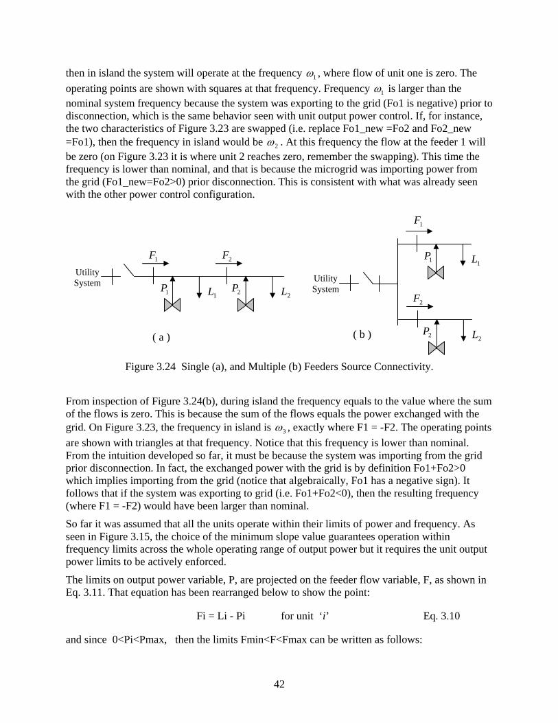
42

then in island the system will operate at the frequency 1ω , where flow of unit one is zero. The operating points are shown with squares at that frequency. Frequency 1ω is larger than the nominal system frequency because the system was exporting to the grid (Fo1 is negative) prior to disconnection, which is the same behavior seen with unit output power control. If, for instance, the two characteristics of Figure 3.23 are swapped (i.e. replace Fo1_new =Fo2 and Fo2_new =Fo1), then the frequency in island would be 2ω . At this frequency the flow at the feeder 1 will be zero (on Figure 3.23 it is where unit 2 reaches zero, remember the swapping). This time the frequency is lower than nominal, and that is because the microgrid was importing power from the grid (Fo1_new=Fo2>0) prior disconnection. This is consistent with what was already seen with the other power control configuration.

Figure 3.24 Single (a), and Multiple (b) Feeders Source Connectivity.

From inspection of Figure 3.24(b), during island the frequency equals to the value where the sum of the flows is zero. This is because the sum of the flows equals the power exchanged with the grid. On Figure 3.23, the frequency in island is 3ω , exactly where F1 = -F2. The operating points are shown with triangles at that frequency. Notice that this frequency is lower than nominal. From the intuition developed so far, it must be because the system was importing from the grid prior disconnection. In fact, the exchanged power with the grid is by definition Fo1+Fo2>0 which implies importing from the grid (notice that algebraically, Fo1 has a negative sign). It follows that if the system was exporting to grid (i.e. Fo1+Fo2<0), then the resulting frequency (where F1 = -F2) would have been larger than nominal.

So far it was assumed that all the units operate within their limits of power and frequency. As seen in Figure 3.15, the choice of the minimum slope value guarantees operation within frequency limits across the whole operating range of output power but it requires the unit output power limits to be actively enforced.

The limits on output power variable, P, are projected on the feeder flow variable, F, as shown in Eq. 3.11. That equation has been rearranged below to show the point:

Fi = Li - Pi for unit ‘i’ Eq. 3.10

and since 0<Pi<Pmax, then the limits Fmin<F<Fmax can be written as follows:

Utility System

1P

1F

1L

2P

2F

2L

1P

1F

1L 2P

2F

2L

Utility System

( a ) ( b )

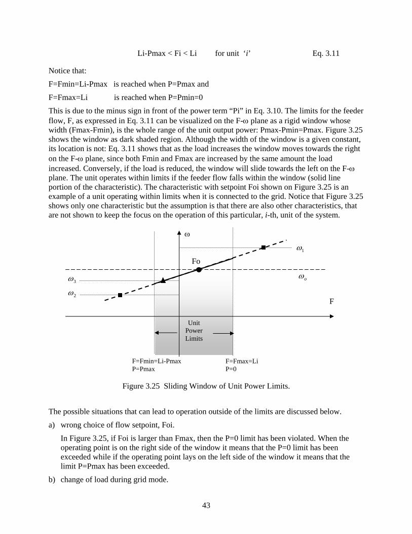
43

Li-Pmax < Fi < Li for unit ‘i’ Eq. 3.11

Notice that:

F=Fmin=Li-Pmax is reached when P=Pmax and

F=Fmax=Li is reached when P=Pmin=0

This is due to the minus sign in front of the power term “Pi” in Eq. 3.10. The limits for the feeder flow, F, as expressed in Eq. 3.11 can be visualized on the F-ω plane as a rigid window whose width (Fmax-Fmin), is the whole range of the unit output power: Pmax-Pmin=Pmax. Figure 3.25 shows the window as dark shaded region. Although the width of the window is a given constant, its location is not: Eq. 3.11 shows that as the load increases the window moves towards the right on the F-ω plane, since both Fmin and Fmax are increased by the same amount the load increased. Conversely, if the load is reduced, the window will slide towards the left on the F-ω plane. The unit operates within limits if the feeder flow falls within the window (solid line portion of the characteristic). The characteristic with setpoint Foi shown on Figure 3.25 is an example of a unit operating within limits when it is connected to the grid. Notice that Figure 3.25 shows only one characteristic but the assumption is that there are also other characteristics, that are not shown to keep the focus on the operation of this particular, i-th, unit of the system.

Figure 3.25 Sliding Window of Unit Power Limits.

The possible situations that can lead to operation outside of the limits are discussed below.

a) wrong choice of flow setpoint, Foi.

In Figure 3.25, if Foi is larger than Fmax, then the P=0 limit has been violated. When the operating point is on the right side of the window it means that the P=0 limit has been exceeded while if the operating point lays on the left side of the window it means that the limit P=Pmax has been exceeded.

b) change of load during grid mode.

Unit Power Limits

F=Fmax=Li P=0

F=Fmin=Li-Pmax P=Pmax

F

ω

oω

Foi

1ω

2ω 3ω

44

In Figure 3.25, if load increases enough, then the window will slide enough of the right side to leave the unchanged setpoint Foi outside of the window itself, on the left side of it. This implies that P=Pmax has been reached, since the load has increased beyond the power capability of the unit. The conclusions are symmetric for the case when the load decreases.

c) transfer to island.

In Figure 3.25, during island the frequency changes and the operating point follows the characteristic. If the frequency of the islanded system is 1ω then the operating point (shown with a square at that frequency) lays outside of the window, on its right side. Then P=0 limit has been exceeded. With a symmetric argument, if the frequency during island is 2ω then the operating point (square) has exceeded the P=Pmax limit.

d) change of load during island mode.

In Figure 3.25, assume that during island mode the frequency settles to 3ω : the operating point is indicated with a triangle at that frequency. The operation is within limits. At this point, if the load increases the window would slide towards the right, and the operating point would lay on the left side of the window since P=Pmax has been exceed. Same symmetric argument holds when load decreases and limit P=0 is exceeded.

The situations (a) through (d) lead to exceeding limits. No matter which case it is, the limit is exceeded because the operating point falls outside the window. All of the situations have in common the fact that if the point is on the right of the window then P=0 is exceeded, if on the left, then P=Pmax is exceeded. This suggests that a steady state characteristic that enforces limits will work for all cases from (a) to (d). Without any loss of generality, only the steady state characteristics that enforce limits when the wrong setpoint is chosen, case (a), will be shown.

Figure 3.26(a) shows the steady state characteristic for a unit that is operating in grid mode with a setpoint Fo that has exceeded the limit P=0. The steady state characteristic is shown with the thick solid line. This characteristic enforces the slope when power P is within the limit, and when the limit is reached, the limit itself becomes the characteristic. This is represented by a vertical line at the value of F=Fmax. This implies that the steady state characteristic holds P=0 while allows the frequency to assume any value that the rest of the units in the system (whose characteristics are not shown in Figure 3.26) will demand. This implies that the frequency would increase, fact shown on Figure 3.26(a) with the arrow on the vertical part of the characteristic. Operation outside of the window is effectively forbidden.

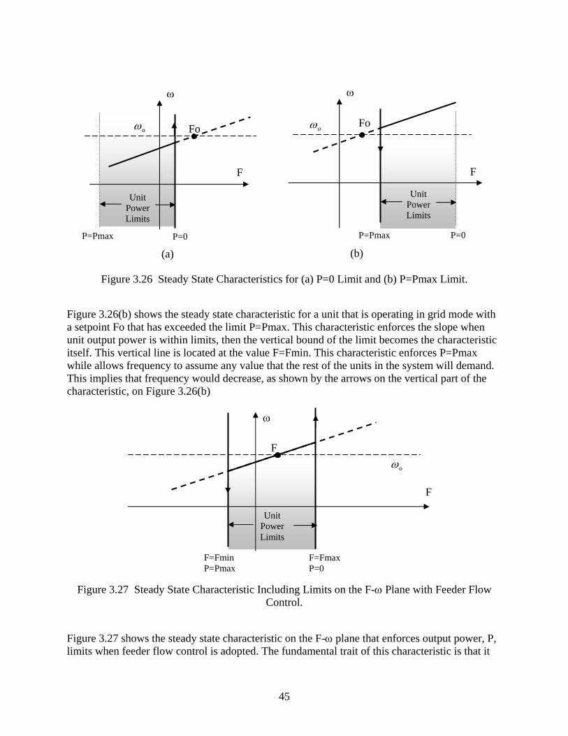
45

Figure 3.26 Steady State Characteristics for (a) P=0 Limit and (b) P=Pmax Limit.

Figure 3.26(b) shows the steady state characteristic for a unit that is operating in grid mode with a setpoint Fo that has exceeded the limit P=Pmax. This characteristic enforces the slope when unit output power is within limits, then the vertical bound of the limit becomes the characteristic itself. This vertical line is located at the value F=Fmin. This characteristic enforces P=Pmax while allows frequency to assume any value that the rest of the units in the system will demand. This implies that frequency would decrease, as shown by the arrows on the vertical part of the characteristic, on Figure 3.26(b)

Figure 3.27 Steady State Characteristic Including Limits on the F-ω Plane with Feeder Flow Control.

Figure 3.27 shows the steady state characteristic on the F-ω plane that enforces output power, P, limits when feeder flow control is adopted. The fundamental trait of this characteristic is that it

Unit Power Limits

P=0 P=Pmax

F

ω

oω Fo

(a)

Unit Power Limits

P=0 P=Pmax

F

ω

oω Fo

(b)

Unit Power Limits

F=Fmax P=0

F=Fmin P=Pmax

F

ω

oωF

46

enforces the slope whenever it lays inside the window, otherwise the bound of the window becomes the characteristic itself. When on this vertical portion, the frequency could assume any value demanded by the remaining sources, shown in Figure 3.27 with the arrows on the characteristic. As the window moves because of changing loading conditions, a different portion of the slope would be enforced, while the vertical parts of the characteristic would have rigidly translated. This enforces the maximum and minimum power limits. The fact that this approach uses a fixed slope (Eq. 3.3) ensures that the frequency will not exceed limits as long as power stays within limits (Figure 3.15).

Figure 3.28 shows the full control diagram, where it is possible to see that the blocks on the upper part belong to the original control structure (as shown in Figure 3.11). The blocks that generate the frequency offsets are in the lower part and represent the change needed to enforce power limits.

Figure 3.28 Control Diagram to Enforce Limits with Feeder Flow Control.

The equation that governs this control has been formally changed from Eq. 3.4 to an equation that keeps into account of changes made in Eq. 3.5 and Eq. 3.6 when respectively dealing with maximum and minimum power limits. The final equation is:

( ) minmax, ωωωω Δ+Δ+−+= iiooi FFm Eq. 3.12

The quantities Δωmax and Δωmin are added to the frequency as calculated in Eq. 3.8. Both quantities are zero when the unit operates within power limits. When Pmax is exceeded, Δωmax becomes negative (never positive) to enforce the limit. When Pmin = 0 is exceeded, then Δωmin becomes positive (never negative) to enforce the limit.

-m

oω

+

s1

)(tVδ ω oF

F

+

_ +

maxωΔ

maxerrPmaxP

+

sKi

0

minerrP

0min =P

+

sKi

0

+

minωΔ

P

47

This control has been implemented in simulation and hardware and the results obtained prove the effectiveness of the control design. The control is tested with all known events that can cause either limit to be exceeded: the hardware results can be all found in Chapter 7.

3.2.3 Mixed System

This Section describes the steady state characteristics for a mixed system consisting of some units that regulate their output power and some other units that control the feeder power flow.

Figure 3.29 shows the steady state characteristics of the controlled power versus frequency. Notice that the controlled power could be output power, P, or feeder flow, F. They are both active powers and have dimensions of kW: that is why it is possible to plot them on the same horizontal axis, “P and F”. On this plane, the sign of the slope is a giveaway of the control being used: negative slope implies unit output control, while positive slope implies feeder flow control.

Figure 3.29 Characteristics on the ”Regulated Power vs. ω” Plane for a Mixed System.

During grid connection the setpoints Po1 and Fo2 are tracked because the frequency is locked to the nominal value, ωo, by the utility. In island the solution will depend on the geometrical configuration of the units on the feeders. This is because when regulating feeder flow the location of the units determines the solution in island, as seen in Figure 3.23 and Figure 3.24. Then, as soon as there is at least one unit regulating feeder flow in the system, the solution in island will depend on the location of the units.

Figure 3.30 shows a possible configuration. The combinations of different configurations could swell to a large number even with few units. For instance, with two only units (one controlling P, other F to have mixed system) there are three independent configurations. The first is with both units on the same feeder, unit controlling F nearest to the utility (as in Figure 3.30), the other

oω

ωω Δ−o

ωω Δ+o

F, P

ω

1ω

01F 02P

Pmax

48

case is when the unit controlling P is the nearest to the utility. The last case is when the two units are in two separate feeders, Figure 3.24(b). The island condition is that grid power is zero, which means that the overall flow in the feeder(s) converging to the utility must be zero. This statement translates on Figure 3.30 with the condition that F1=0 in island, since that is the only one feeder connecting to the grid. This implies that for the unit configuration shown in Figure 3.30, in island mode the operating point is at frequency 1ω , lower than the system frequency only because the flow Fo1 is positive (importing power during grid connection). A negative value for Fo1 would have generated an intersection with the axis F=0 at a frequency higher than nominal.

Figure 3.30 Mixed System on a Single Feeder, with Flow Control Near the Utility.

Values of output power could exceed limits for the same reasons separately seen in the previous sections: load change during island and grid, wrong setpoint choice, transfer to island. The characteristics of Figure 3.29 will need to include features that will enforce limits during steady state.

The value of P at the frequency 1ω in Figure 3.29 is the amount of power generated by the unit that controls output power. Figure 3.15 with fixed slope, represents the limits for the output power in the mixed system: this is a rigid characteristic (i.e. does not translate on the P-ω plane). In Figure 3.15 the constant value used for the slope guaranteed that frequency is within limits as long as power is held within its own limits.

The unit controlling feeder flow, F, needs to enforce output power limits as it was described on Figure 3.27. Only a window (Pmax wide) of the slanted slope is taken. The location of this window [Fmin, Fmax] varies because it depends on the value of the loading condition, as shown in Eq. 3.10. The overall loading conditions are determined by the loads and the generations behind the unit. In Figure 3.30 the total loading condition (Lt) of the first unit (Lt1) includes also the other load (L2) and second unit power output (P2) as a negative contribution to the overall loading. From Figure 3.30 it is possible to write:

F1 = Lt1-P1

Lt1=L1+L2-P2

This is to show that the physical location of the window that represents the limits on the feeder flow may depend not only on the values of the loads, but also on the instantaneous amounts of power output of other units. The point is that no matter where the sliding window is located, the

1P

1F

1L 2P

2F

2L

Utility System

Unit 1 Regulating Flow F1

Unit 2 Regulating Output P2

49

characteristic will coincide with the slanted slope inside the limits and will become vertical as the limits are reached, as per Figure 3.27.

Figure 3.31 shows the steady state characteristics that enforce output power limits for a mixed system consisting of one unit controlling output power, P, and other unit controlling feeder flow, F.

Figure 3.31 Steady State Characteristics Including Limits on the Regulated Power vs. Frequency Plane, with a Mixed System.

Figure 3.31 shows that the unit regulating output power has a rigid steady state characteristic, while the unit regulating feeder flow has a sliding steady state characteristic, here shown in a generic position. Figure 3.31 shows also that all the characteristic have the same slope. Units controlling F and P have the sign reversed in the slope, but the magnitude of their slopes are identical. If this magnitude is chosen as of Eq. 3.3, equal to the minimum slope, then it was seen that as long as the power is within limits, then also the frequency is guaranteed to stay within limits. Then it follows that the steady state characteristics shown in Figure 3.31 enforce both limits on power and frequency when fixed minimum slope is used in all units of the mixed system.

oω

F, P

ω

1ω

01F 02P

P2=Pmax

F1=F1max P1=0

F1=F1min P1=Pmax

P2=0

50

Chapter 4. Interface of Inverter to Local System

This chapter describes how the ratings of the several components within a microsource need to be coordinated to achieve the desired operation. Figure 4.1 shows the full layout of every component that appears in a microsource: from left to right, there is the prime mover responsible to generate a DC voltage, then there is the DC bus that needs to include some storage. The inverter is the interface between the DC bus and AC system and is responsible for the operations of the microsource. Immediately connected to the inverter terminals there is an L-C filter bank to eliminate the higher harmonic from the voltage waveform and then there is the inductor that determines how active and reactive power can be dispatched. The final connection with the feeder is achieved by means of a delta-wye transformer with a neutral connection to allow for single phase loads to be connected to the system.

Figure 4.1 Microsource Component Parts.

All these components need to be coordinated and selected in such a way that their ratings are compatible with the capabilities of the other components of the chain.

4.1 Prime Mover Dynamics and Ratings The prime mover is the block that converts the chemical energy of the fuel in DC electric power. Some examples of prime movers are microturbines and fuel cells. Each prime mover has a dynamic response to changes in power command that depends on the technology adopted. In general the dynamic response takes from few seconds to few minutes to track a step change in the power command, for example Capstone microturbine shows a time constants in the order of 10-20 seconds to follow a step change in the power command in Figure 4.2, while a fuel cell stack takes minutes to track the power command. There is the need to provide some form of energy storage to ensure that the energy for the loads is immediately available. The storage will be located at the DC bus. The rating on the prime mover is given in terms of maximum active power output, which is the largest amount of power that the generator can convert to electric form. This is an upper limit that will influence the choice of the ratings for other components of the microsource such as the inverter and the transformer. Usually, the prime mover has also a

FilterC

+ Prime Mover

X

Voltage Sourced Inverter DC interface Prime Mover

Inductor

FilterL

Transformer

Filter

4 Wire Feeder

N

51

rating on the voltage output, establishing the maximum voltage level at which that the power is produced.

Microturbines have a two pole permanent magnet generator that converts the mechanical power of the shaft into electric power at variable frequency, depending on the speed of rotation. The variable frequency voltage is rectified to a DC voltage that is almost independent of the variable AC frequency.

Figure 4.2 Capstone DC Bus Voltage During Load Changes in Island Mode.

Figure 4.2, [21] shows the behavior of the DC bus voltage during load changes on a Capstone microturbine operating in island mode. Each time the electrical load is diminished, the DC bus voltage immediately increases due to the lower power demand: at that point the fuel valve controller decreases the fuel to the microturbine to reduce its output power and regulate the DC voltage. When the load is increased, the DC voltage decreases because the storage is providing immediately power to the load: at this point the controller increases the fuel injection to the microturbine to increase its output power and restore the DC voltage. DC bus voltage is 760V and excursions in either direction never exceed 3 volts, suggesting that the range of voltages on the DC bus is independent of the angular speed of the microturbine shaft.

The fuel cells have a different behavior on the DC voltage output as a function of the output power. For example, Figure 4.3 [24] shows the stack voltage as the current output increases on a 3.5kW fuel cell stack: the voltage changes of almost of 1 Volt per Ampere for the first 10 A, then it changes with a smaller slope.

52

Figure 4.3 Fuel Cell Stack Voltage as a Function of the Output Current.

The bottom line is that the voltage changed of about 20V as the output current went from zero to 50A, out of a 68V no-load voltage. This characteristic implies that the output voltage of the DC stack needs to be interfaced with a DC/DC converter with the DC bus voltage. Without such an interface when the fuel cell output voltage becomes smaller than the voltage of the DC bus the power would flow in the opposite direction towards the stack.

4.2 DC Bus and Storage Ratings The DC bus has two ratings, one is on the voltage, the other is on the amount of energy that can be stored in it. The DC bus voltage rating is the voltage level from the prime mover. Microturbines have a 3 Volts range on a 760V, while fuel cells need to be interfaced with a DC/DC converter to obtain such a small range of change in the output voltage as the loading conditions change. The voltage from a 35kW fuel cell would require a series of 10 stacks like the one showed on Figure 4.3 reaching a no load voltage output in the range of 700V before the DC/DC converter.

Since the prime mover does not have instantaneous tracking capability of the power command, the DC bus needs to store enough energy to be able to supply the load immediately while the prime mover ramps up. The worse case is during island operation when the grid is not available to supplement that transient energy. The amount of rated stored energy should be enough to guarantee tracking load requests in the face of the slow dynamics of the prime mover. This implies that the ratings on the storage are dependent on the technology of the prime mover, for instance, a microturbine that takes ten seconds to ramp up output power should have less storage than a fuel cell that takes over a minute to ramp up.

53

Figure 4.4 Replacement of Prime Mover + DC Storage with DC Source.

With storage, the value of the voltage at the DC bus is quite stiff because it is regulated by the prime mover. Since there is a need for some sort of available storage, then it is possible to eliminate the prime mover altogether from the model, without loss of generality. Figure 4.4 shows how the prime mover + DC storage blocks can be replaced by a DC voltage source. This simplification is legal because the two parts in the dark dashed ovals behave essentially the same. This simplification allows to obtain conclusions on the behavior of inverter based sources, without having the need to use an actual prime mover. The hardware tests that will be described in the following chapters adopt a microsource that takes advantage of this simplification.

4.3 Sizing the Coupling Inductor, Inverter Voltage and Power Angle

Microsources need a power electronics block to perform the DC/AC conversion to interface with the local grid where they are installed. The inverter terminals are ultimately connected to the AC system by means of an inductance. Figure 4.5 shows the details of the interface with the grid. Measurements are taken from both sides of the inductance and a controller generates desired values for V and δv to track the externally commanded values for active power injection P, and voltage magnitude E at the point of connection with the grid.

I

E VGenerator

X

P,Q

Voltage Sourced Inverter DC StoragePrime Mover

AC Interface

I

E V+

X

P,Q

Voltage Sourced Inverter DC SourceAC Interface

54

Figure 4.5 P and Q as a Function of the Voltages and their Angles.

The size of the inductor is derived from the inverter voltage ratings, the regulated bus voltage and the limits on the power angle. The power angle is the angle difference between the voltages at the inverter and the regulated bus. Typical limits can be:

- Limit on V (such as Vmax .≤ 12 pu ). This condition is dictated by the value of the voltage at the DC bus and by the kind of power electronic bridge used in the inverter.

- Limit on δ (such as reesdeg 30max ≤δ ). This condition derives from the need for the controller to operate in the linear portion of the P( δp ) characteristic: as Figure 4.6 shows, 30 degrees is a reasonable choice for the maximum value for δp .

Figure 4.6 Power-Angle Characteristic.

The power angle characteristic is already a great place to start to limit the size of the inductor, because it provides some upper and lower boundaries for its value. If the value of the inductance is too large, then the resulting angle at maximum power would not satisfy the condition of

AC Grid

V v∠δ E E∠δ

XL

P,Q

δ δ δ

δ

δ

p v

p

p

E

L

L

PVEX

QV VE

X

= −

=

=−

sin( )

cos( )2

Inverter

55

linearity. A value of 30 degrees provides a 4% error in the linear approximation, but a maximum power angle value of 10 degrees implies that the largest error in the approximation would be 0.5%. A smaller range for the power angle would require too much precision in the synthesization of the angle at the inverter terminals. The inverter synthesizes the voltage angle with a certain tolerance depending on the switching frequency. The higher is the operating frequency the lower is this tolerance. If a large range for the power range is chosen, then the relative size of the error is small and there are no problems in injecting power. If a small range is chosen, then the same absolute value of the tolerance becomes relatively large compared to the range of delta, implying problems in achieving constant power injection. The power would oscillate, and if the range for the angle is chosen really small, say a fraction of a degree, then it would be nearly impossible to regulate power due to the fact that the angle would need to be held with a very high precision.

4.3.1 P versus Q Area of Operation

When designing the inverter, the choice of ratings of the devices plays a key role. The power electronic block at the minimum has to be rated as the prime mover. If the ratings of the prime mover exceed the inverter ratings then when the prime mover operates at peak power it would be impossible to transfer its full power. Each inverter has limits dictated by the ratings on the silicon devices. These limits appear in the form of maximum voltage that the power electronic device can safely sustain and the maximum current that it can carry. Based on these considerations, each designer provides a range of active and reactive powers that the inverter can safely operate at. At this point there is the first formulation of the answer for the problem of the size of the inductor:

The size of the inductor must be such that it enables delivery of the active and reactive power that the inverter can provide.

Figure 4.7 shows the plot of the active and reactive power obtained from the formulas included in Figure 4.5 as a function of the inverter and bus voltage, their angle difference and the impedance. All quantities are in per unit to maintain generality and the plot is obtained for the power angle equal to 15 degrees. Smaller inductances allow larger power flows. The inductor should be chosen small enough to guaranteed deliver of the specified amounts of power: if the inductor is chosen too large the power may no longer be deliverable. The optimal inductor size can be seen as the maximum size that the inductor can have, and still being able to satisfy the delivery requirements.

To develop some intuition on how to solve the problem it is useful to build some maps of the power that it is possible to deliver given the limits that need to be satisfied.

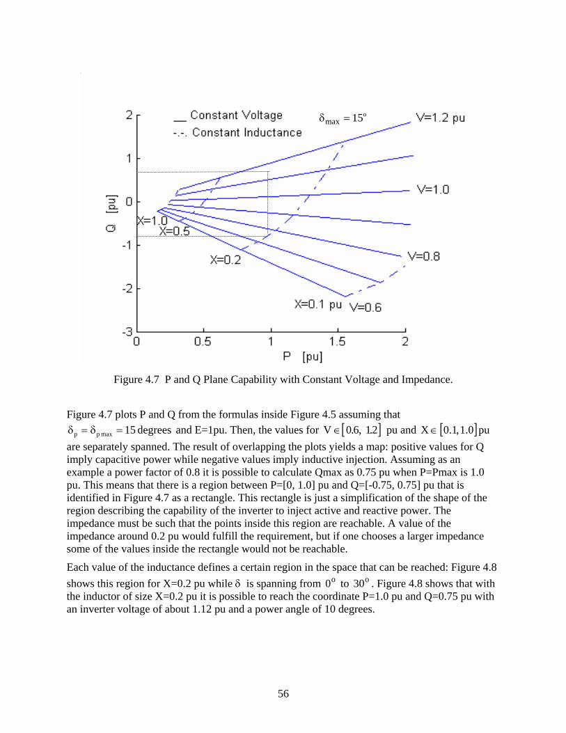
56

Figure 4.7 P and Q Plane Capability with Constant Voltage and Impedance.

Figure 4.7 plots P and Q from the formulas inside Figure 4.5 assuming that degrees 15max pp =δ=δ and E=1pu. Then, the values for [ ]V ∈ 0 6 12. , . pu and [ ]pu 1.0 ,1.0X ∈

are separately spanned. The result of overlapping the plots yields a map: positive values for Q imply capacitive power while negative values imply inductive injection. Assuming as an example a power factor of 0.8 it is possible to calculate Qmax as 0.75 pu when P=Pmax is 1.0 pu. This means that there is a region between P=[0, 1.0] pu and Q=[-0.75, 0.75] pu that is identified in Figure 4.7 as a rectangle. This rectangle is just a simplification of the shape of the region describing the capability of the inverter to inject active and reactive power. The impedance must be such that the points inside this region are reachable. A value of the impedance around 0.2 pu would fulfill the requirement, but if one chooses a larger impedance some of the values inside the rectangle would not be reachable.

Each value of the inductance defines a certain region in the space that can be reached: Figure 4.8 shows this region for X=0.2 pu while δ is spanning from 0o to 30o . Figure 4.8 shows that with the inductor of size X=0.2 pu it is possible to reach the coordinate P=1.0 pu and Q=0.75 pu with an inverter voltage of about 1.12 pu and a power angle of 10 degrees.

o15max =δ

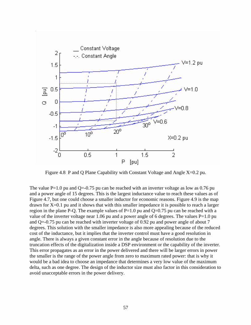
57

Figure 4.8 P and Q Plane Capability with Constant Voltage and Angle X=0.2 pu.

The value P=1.0 pu and Q=-0.75 pu can be reached with an inverter voltage as low as 0.76 pu and a power angle of 15 degrees. This is the largest inductance value to reach these values as of Figure 4.7, but one could choose a smaller inductor for economic reasons. Figure 4.9 is the map drawn for X=0.1 pu and it shows that with this smaller impedance it is possible to reach a larger region in the plane P-Q. The example values of P=1.0 pu and Q=0.75 pu can be reached with a value of the inverter voltage near 1.06 pu and a power angle of 6 degrees. The values P=1.0 pu and Q=-0.75 pu can be reached with inverter voltage of 0.92 pu and power angle of about 7 degrees. This solution with the smaller impedance is also more appealing because of the reduced cost of the inductance, but it implies that the inverter control must have a good resolution in angle. There is always a given constant error in the angle because of resolution due to the truncation effects of the digitalization inside a DSP environment or the capability of the inverter. This error propagates as an error in the power delivered and there will be larger errors in power the smaller is the range of the power angle from zero to maximum rated power: that is why it would be a bad idea to choose an impedance that determines a very low value of the maximum delta, such as one degree. The design of the inductor size must also factor in this consideration to avoid unacceptable errors in the power delivery.

58

Figure 4.9 P and Q Plane Capability with Constant Voltage and Angle X=0.1 pu.

It must be noticed that there are several choices of the impedance that allow to deliver the P and Q inside the region, but each choice corresponds to a different inverter voltage and power angle. For what concerns the maximum inverter voltage, it can be noticed that with X= 0.2 pu, in Figure 4.8, there is a need to have a 1.12 pu inverter voltage to reach the coordinate P=1.0 pu, Q=0.75 pu. With X=0.1 pu the inverter voltage needs to be only 1.06 pu. It is manifest how the choice of the impedance affects the requirements on the inverter to reach the P and Q coordinates. For instance a lower DC bus voltage can be afforded when using X=0.1 pu rather than X=0.2 pu. The ideal design must keep into consideration the issue of DC bus magnitude because it is directly connected to the maximum voltage that the inverter can achieve. The inductance also affects the value of the minimum voltage that the inverter may need to synthesize when trying to reach high values of inductive reactive power. But this value is less critical because it can always be reached by means of a thinner modulation of the voltage waveform: on the contrary, the maximum voltage represents a real issue because its value determines the rating that the DC bus must have.

In summary, a smaller size of the inductor corresponds to a lower cost, a lower requirement on the DC bus rating and a smaller range of power angle. The range of the power angle cannot be allowed to get too small to avoid errors in the power to become unacceptable. A compromise between angle resolution, inductor price and DC bus rating is key to obtain an ideal match between inverter capabilities and inductor.

59

4.4 System Ratings

The inverter performs the task of converting the voltage from a DC level to the AC utility frequency. The output voltage level of the inverter is a free variable that can be changed with an appropriate choice of the turn ratio of the transformer. The inverter allows the flexibility of adopting a wide variety of prime movers. The output voltage of the inverter depends on the DC bus voltage and the modulation technique adopted.

The inverter needs at the minimum to have enough ratings to supply the active rated power of the prime mover, but the final ratings need to be somewhat higher to be able to supply the reactive power necessary for voltage regulation. The silicon devices inside the inverter have thermal limits that need to be observed to guarantee their operation. These thermal limitations are translated in a maximum amount of continuous operation current that the devices can withstand without incurring in thermal runoff and being damaged. During faults the silicon can transiently sustain a 2 pu current for those few cycles that the protection takes to intervene and disconnect the source.

It is possible to show how the maximum current on the device impacts the AC side rms current value. Assuming a power factor of 0.8 it is possible to calculate that the maximum reactive power injection is:

( )( ) ( )( ) P 75.0PFcosatanPtanPQ

cosPF==ϕ=

ϕ=

When the inverter is operating at the maximum current output the voltage of the inverter will also be nearest it maximum possible value. This means that the modulation of the DC voltage has become very wide: to greatly simplify the analysis a six pulse operation of the bridge is assumed. This implies that each of the devices conduct for a half of the fundamental frequency period. Figure 4.10 shows the voltage source inverter that interfaces the DC bus voltage with AC sinusoidal current sources. These sources are assumed to be 120 degrees apart in each phase.

Figure 4.10 Voltage Source Inverter.

The fundamental frequency AC side voltage magnitude is related to the DC voltage by the following expression [6]:

6

5

4

3+

C

B

A

VDC

1

2

N

Ic(t)

Ib(t)

Ia(t)

DCI

60

DCrms

nl V2Vπ

=−

Equaling the active power in the AC and DC side, it is possible to observe that the currents in the AC and DC side are related by:

( )

( )ϕπ

=

ϕ=== −

cosI23I

cosIV3PIVP

rmslineDC

rmsline

rmsnlACDCDCDC

This expression shows that only the component of the AC current that is in phase with the voltage waveform is reflected to the input of the inverter, at the DC side. Figure 4.11 shows the voltage between the points A and N illustrated in Figure 4.10. It shows what switching sequence has to be applied to achieve each of the six pieces of the voltages: each devices conducts for 180 degrees. Figure 4.11 also shows what current flows in the DC bus given the switching sequence. Depending on the phase of the current on the AC side with the voltage Van, then it is possible to see that the current seen on the DC side changes. The first case shows the current Ia in phase with the voltage Van: the power factor is one and all the AC current is used to exchange power with the DC side. The second case shows a current 90 degrees apart with the voltage: the power factor is zero and none of the AC current is used to exchange power with the DC side. In fact, it is possible to see that the current is entering the DC bus for 30 degrees and leaving for the remaining 30 degrees with a zero net effect. In this case only reactive power is exchanged with the AC side. The last case shows the current with a phase displacement equal to the chosen PF of 0.8 where AC voltage and current waveforms are displaced by:

o86.38)PFcos(a ==ϕ

This case represents a contemporary exchange of active and reactive power with the AC system.

61

Figure 4.11 AC and DC Currents on the Voltage Sourced Inverter.

The apparent phase of the inverter is given by:

rmsline

rmsnl IV3S −=

This last expression when combined with the expression for the active power allows to give a value for the inverter ratings starting from the value of the power of the prime mover and the power factor chosen:

( ) PFP

cosPS Mover imePrDC =

ϕ=

The maximum output power of the prime mover is the maximum active power that the inverter may ever be requested to deliver, while the maximum amount of reactive power that is injected is determined by the choice of the power factor.

The transformer has the task to interface the three-phase world of the inverter terminals with the 4 wire environment on the feeder side to allow for single phase loads to be connected. The delta configuration on the inverter side of the transformer is a direct consequence of the fact that the inverter generates voltage on a line to line basis between phases. The feeder side of the transformer is wired at wye, with the center of the star available to be connected to the neutral

Van

Ia

Ia

Ia

Only Active Power

Only Reactive Power

PF=0.8

146 Switching Sequence

AC Current Flowing in

DC Bus

235 136 236 245 145

Ia -Ib -Ic Ib -Ia Ic

62

cable of the 4 wire system inside the microgrid. Due to the connectivity of the transformer secondary, any kind of load can be connected on the feeders of the microgrid: three phase loads connected at delta or wye and single phase loads between a live phase and the neutral such as commercial appliances.

The transformer provides electrical insulation between the voltages on the feeder and the voltages of the inverter side through the magnetic coupling of the coils. The choice of the delta to star connectivity provides also a filter for the zero sequence currents that may flow in the feeder due to a fault: this provides the power electronic devices of the inverter with a level of protection from faults.

Figure 4.12 Transformer Current During Fault on a) Wye Side, b) Delta Side.

Figure 4.12 shows the line currents flowing on the wye and delta side as a consequence of a single line to ground fault on the feeder side without the intervention of protections to open the circuit. For ease of comparison, the transformer has a unitary turn ratio resulting in same line current magnitudes on either side. Normal loading conditions determine a current of about 50A, but as soon as the fault is applied the currents on the wye side reach over 400A in the faulted phase, while on the neutral cable that provides the return path for the sum of the three line currents, the faulted condition determines almost 900A, Figure 4.12a. On the delta side, the line currents corresponding to the currents flowing in the inverter legs can be seen to barely exceed the 200A value in Figure 4.12(b). The voltage of the faulted phase on the feeder side will be zero due to the fault to ground, but due to the wye-delta connectivity two of the voltages on the delta side will be 88 percent of the original values while the third line to line voltage will be 33 percent of the nominal value [7]. With the introduction of the transformer a voltage sag on the inverter side will never be lower than 33 percent of the nominal value with any kind of single line to ground faults.

The transformer creates a free variable out of the DC bus since any voltage at the inverter terminals can be interfaced with the feeder voltage by an appropriate choice of the turn ratios. The ratings of the transformer must be enough to transfer all the active and reactive power that is

(a) (b)

63

generated by the inverter: the VA ratings of the transformer must be equal or larger than the ratings of the inverter.

64

Chapter 5. Unbalanced Systems

This chapter addresses the fact that unbalanced conditions of small magnitude are a relatively common operation of the system and the microsources need to be able to operate in this environment. The reasons that determine unbalance are first given. An active approach at eliminating unbalance determines higher requirements in the ratings of the source. The microsource needs to operate in the unbalanced environment without attempting to restore balanced conditions.

5.1 Reasons that Determine Unbalance Microgrids need to operate under unbalanced conditions due to the fact that electrical systems naturally have some degree of unbalance. There are many reasons why the supply voltage may have unbalance, for instance the geometrical configuration of conductors in overhead transmission lines. The conductors on the towers are swapped every so many miles to minimize the effect of the asymmetric mutual coupling between the conductors and the ground, but nonetheless there is always some residual asymmetry left that determines unbalance. Another cause of unbalance is the insertion of three phase loads with unbalanced impedances: a delta load that draws unbalanced currents will determine positive as well as negative sequence components in the voltage across the system. An unsymmetrical placement of single phase loads between phases and neutral determines not only negative, but also zero sequence component due to the fact that the currents in the neutral do not sum up to zero anymore. Single phase loads across feeders are already distributed evenly on the three phases as much as possible to avoid problems of unbalance, but complete symmetry is nearly impossible to guarantee, more so in the face of the uncertainty of what loads are inserted and when. A distant fault outside the microgrid somewhere in the utility system is also responsible for unbalanced voltages at point of common coupling.

Transformer connectivity can help to mitigate the effects of unbalance. Delta-wye transformers, with the delta side on the utility side are common practice in the distribution system. An advantage of this transformer is that it traps the zero sequence currents in the delta side allowing only the positive and negative to pass through. Another advantage is that a given voltage sag on the primary propagates through the windings of the transformer as a smaller voltage sag on the secondary. For instance, a single line to ground fault on the primary of a delta transformer would create a 100 percent sag on the faulted phase, but on the wye connected secondary of the transformer the voltage will sag at most at 33 percent on the line to line while sagging at most 58 percent on the line to neutral [7].

There are several effects to unbalance, for instance induction motors will have an induced torque component at twice the system frequency. This is because the negative sequence will generate a torque in the opposite direction of the one generated by the positive sequence. Unbalance has detrimental effects on the machine, for instance it increases the heat generated in the resistive coils of the rotor that sees a field rotating at a relative speed that is twice the rotor speed, inducing high currents. Also, there are mechanical stresses on the bearings due to the pulsating term in the torque.

The voltage unbalance is defined in Appendix D of ANSI Standard C84.1-1989 [8] as:

65

voltageaverage

voltageaverage fromdeviation maximum 100 unbalance voltageof % =

This standard requires that electrical supply systems should be designed and operated to limit the maximum voltage unbalance to 3 percent when measured at the point of common coupling under no load conditions. ANSI states that approximately 98 percent of the utilities surveyed are within this limit, with 66 percent within 1 percent unbalance. To comply with the ANSI standard, National Electrical Manufacturers Association (NEMA) [9] requires that a motor needs to be derated by a factor of 0.9 to be able to withstand the currents at the negative sequence without exceeding the nameplate ratings.

5.2 Unbalance Correction When a voltage unbalance exceeds the nominal value that can be tolerated within a system as stated by the ANSI standard, some corrective action must be taken to prevent this unbalance from creating problems in the operation of the equipment inside the microgrid.

One approach could be to inject sequence currents from the inverter to rebalance the system. The inverter can only generate voltages on a line to line basis, so the scope of the correction would only be limited to the negative sequence. The measures of voltages and currents that are passed to the control need to be conditioned to identify the positive and negative sequence components. Each of the components is then separately controlled: the positive sequence quantities are regulated to the externally requested values while the negative sequence quantities are regulated to zero. The structure of the control needs to be more complex and the ratings of the inverter need to be augmented to be able to carry the negative sequence currents.

Another approach is to transfer to intentional islanding mode by separating the microgrid from the utility in the case that the unbalance exceeds the tolerable levels. This solution does not require any modifications in the control and the microsources only need to be able to correctly operate under unbalanced conditions as long as the level of unbalance is below a determined threshold. In this case the sensing equipment at the point of interconnection with the grid needs to be able to evaluate the unbalance and send a tripping signal to the static switch when limits are exceeded. This solution does not require any extra rating of the inverter to allow for the negative sequence current injection.

5.3 Operation Under Unbalance The inverter ratings need to be increased by a large factor to correct for sustained voltage unbalances. Avoiding the active cancellation of negative sequence implies that the static switch needs to be able to selectively disconnect the microgrid when unbalances exceed the tolerance level of 3 percent as recommended by the ANSI standard. This approach implies that the basic control of the microsource needs to be able to correctly operate in an environment that may contain unbalances up to that tolerance. Unbalances affect the basic control because the opposite rotating negative sequence introduces 120Hz oscillations in the measure of power and voltage magnitude. The measurement system assumes quantities with positive sequence component only: when unbalances are present some calculations are affected. For instance, the d-q stationary components will no longer be represented by two vectors of same magnitude and phase. When plotted on the d-q plane these components will not describe a circle but an ellipse. The

66

instantaneous calculation of the radius of the ellipse (the magnitude of the voltage) will yield a quantity pulsating at twice the nominal system frequency. If the unbalance is less than 3 percent, the magnitude of the pulsation can be very small. The active power measure will have the same issue, showing a small amplitude ripple at twice the system frequency superimposed over the traditional value.

Filtering the signals of voltage magnitude and power is the solution that can eliminate the presence of the small ripples. In the hardware realization measures are brought in by sensing equipment and translated to digital values. These values are plagued by noise coming from the sensing devices and from the connecting cables that carry those measurements. The digital values inside the DSP environment need to be filtered to minimize the effect of these noises. It turns out that those filtering levels may also be enough to eliminate the 120Hz ripples in the measures due to low levels of unbalance present in the system. In the hardware laboratory setup the voltage supply is rather well balanced, showing a 0.2 percent level of unbalance at the 480V point of common coupling.

The values of P,Q and regulated voltage magnitude, V are filtered before being introduced in the controller. The filter is a low pass, single time constant transfer function:

s

sH1

1)(τ+

=

The time constant τ is worth 30ms, for P, Q and V. Figure 5.1 shows the frequency response of this filter.

Figure 5.1 Filter Gain as a Function of Frequency.

The test system is one microsource in island connected to an unbalanced load. The load is unbalanced by removing the connection at one of the three phases. As a consequence, the current in that particular phase will be zero. The resulting unbalance in the voltage is 5.12%.

67

Figure 5.2 shows the plots for P,Q and V as the unbalance is applied. It is possible to notice the 120Hz component superimposed to the balanced value on each of the three quantities. The voltage magnitude, V, shows a very small magnitude in the double frequency component, that is because the unbalance driving it is 5.12%. The values of P and Q show a relatively larger magnitude in the double frequency component because they are calculated using voltage and as well as the current, which has a 100% unbalance.

Figure 5.3 shows the three line to line voltages at the load terminals (upper traces) and the currents (lower traces). Figure 5.4 shows the same quantities with a longer time division (1s/div) to make the point that there are no lower frequency oscillations in the envelope of the voltages or currents.

Figure 5.2 P, Q and Magnitude of V. [50ms/div]

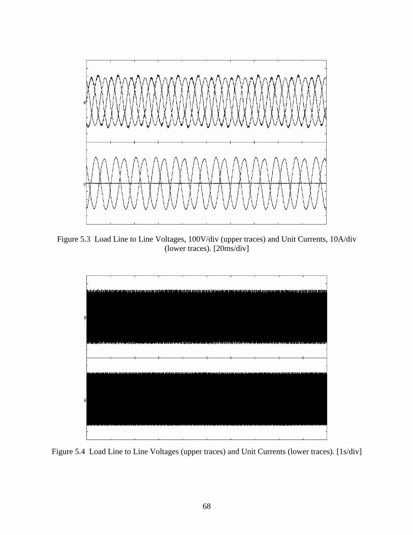
68

Figure 5.3 Load Line to Line Voltages, 100V/div (upper traces) and Unit Currents, 10A/div (lower traces). [20ms/div]

Figure 5.4 Load Line to Line Voltages (upper traces) and Unit Currents (lower traces). [1s/div]

69

Figure 5.5 shows the measures of P and Q as well as the measure of V at unit 1 when unit 1 is operating in parallel to unit 2. The unbalance is determined by a phase on the load of unit one being open. The overall voltage unbalance at the terminals of unit 1 is reduced to 3.97% due to the presence of unit 2. Figure 5.6 shows the same quantities for unit 2. Being that this second unit is farther away from the unbalanced load, the amplitudes of the oscillations at 120Hz are reduced.

Figure 5.5 Unit 1 - Two Units in Parallel. [50ms/div]

70

Figure 5.6 Unit 2- Two Units in Parallel. [50ms/div]

Figure 5.7 shows the 120Hz ripple at the measured quantities of the microsource when this unit is connected to the grid and the unbalance is created by the opening of one phase. In this case the voltage unbalance measured at the terminals of the unit is of 2.82%. This is because of the stiff Thevenin impedance of the utility system being in parallel to the unbalanced load at the source. The oscillations on P and Q have a very low magnitude, while the oscillations on V have nearly completely disappeared. This allows to conclude that the source does not require any active action to compensate for negative sequences, as it has been shown that it can safely operate under the voltage unbalances below the threshold of tripping.

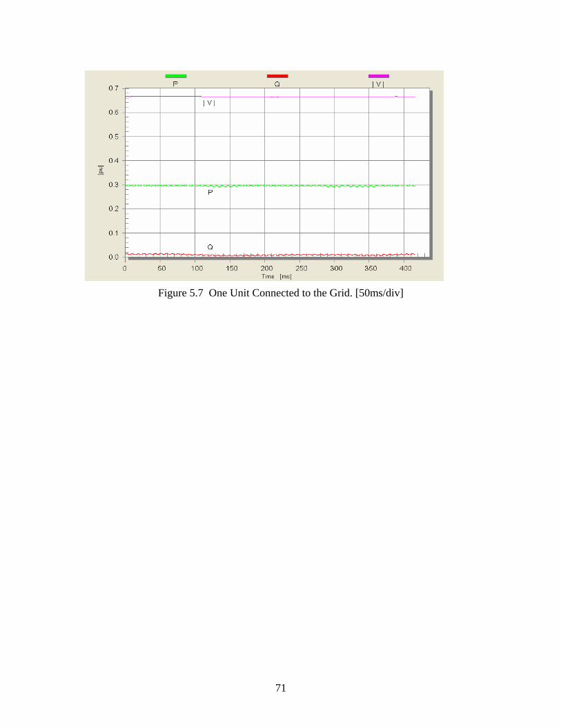
71

Figure 5.7 One Unit Connected to the Grid. [50ms/div]

72

Chapter 6. Hardware Implementation

The ultimate validation of the control capabilities is a successful series of tests carried on a hardware level. Steady state and dynamic analysis can give many insights on the performance of the control, but it is only after realizing a scaled down version of a microgrid that it is possible to assess the actual quality of the design.

The details of the hardware setup that implements the proof-of-concept for the microgrid will be given in this chapter.

6.1 Basic System A scaled down version of a microgrid has been reproduced in the lab to test microsource operation and control. This system incorporates the typical components that can be found in a local load center: there is one transformer that connects to the utility system and a radial network with feeders that delivers the electric power to all the loads. Figure 6.1 shows the network configuration. The point of delivery of power from the main grid is at 480 V, while inside the system all the loads and the feeders are operating at 208 V. The microsources generate power at the voltage level of 480 V appropriately lowered to the network voltage by a separate transformer. On the inverter side of the transformer there is a low pass LC filter to smooth out the voltage waveform. In series to the filter there is an inductance to allow for power transfers. There are two load centers located near the two microsources and another load electrically installed between the two units: this allows to test the power sharing during operation in island mode.

Figure 6.1 Single Phase Test System Diagram.

The three phase passive loads are connected at star and are purely resistive, while the cables consisting of four conductors, three phases and a neutral, that run in parallel from a bus to the next, representing the feeder.

1MS 2MS

4 wire Cable

4 wire Cable, 75 yd

4 wire Cable, 25 yd

Load Load Load

Utility System

208 V

480 V

Static Switch

73

Microsources are connected to the local feeder with a transformer in series to an inductance. The connection is at delta on the inverter side and at wye on the feeder side with the center star connected to the neutral wire of the feeder cable. The voltage level of the feeder is 208V, while the inverter operates with voltages of 480V. In summary, operations are on a three wire environment on the inverter side of the transformer, while they are on a four wire environment on the microgrid.

Figure 6.2 shows the basic equipment that appears in a microsource: the inverter is connected to an ideal DC source and creates the AC voltage at its three phase terminals. The inverter is controlled by the gate signals that are generated by the control blocks. The controller uses the measures of voltage and current at the feeder, where the unit is installed. When the unit is controlling the feeder power flow, then the current from the feeder on the side leading to the grid are also fed back to the control. The microsource is connected to the feeder with a transformer to lower the voltage from 480V to 208V. The inverter side is connected to delta, while the lower voltage side is star connected, with the neutral of the transformer carried on in the feeder to allow for single phase loads to be connected.

Figure 6.2 Single Phase Diagram of Inverter Connection to the Feeder.

6.2 Description of the Laboratory System

This section describes in detail the constituent parts present in the hardware circuit. The overall single phase circuit diagram is represented in Figure 6.3. Somewhere in the building there is a connection that can be considered a stiff voltage source, representing the utility system. From that connection, there is a three wire cable (Z1) that reaches the transformer T1, located in the laboratory. This transformer has the neutral connected to the fourth wire of the system that runs in parallel to every feeder. On the microgrid side of the transformer there is the static switch to connect and disconnect from the grid. Then there is a short 4 wire cable (Z2) that connects to the first microsource (MS1) and load center (L1). From there a 75 yd, 4 wire cable (Z3) reaches an intermediate load center (L2). The last 25 yd of cable (Z4) reach the second microsource (MS2) and the last load center (L3).

FX

FC

)t(vabc

+

VDC Inverter

Controller

LocalFeeder

Gate Signals

X

)t(i)t(e

abc

abc

480 V 208 V

n

Towards Grid

Feeder Currents )(tiabc

FX

74

Figure 6.3 Single Phase Laboratory Circuit Diagram.

Each microsource is connected to the feeder by a series of low pass LC filter, an inductor and a transformer. The 208V low side of the transformer is connected at wye with the neutral cable connected the fourth wire inside the system. The 480V high side of this transformer is on the microsource side where there is a 3 wire system. The supply voltage from the utility is also at 480V, while the rest of the microgrid operates at 208V.

Every component of the network is described in detail in the following paragraphs.

6.2.1 Transformers This section describes the transformers used in the systems. The transformer that is used to connect with the utility system has larger ratings than the transformer used to interface with the microsource. The two microsources are twin systems, therefore their transformers will be identical.

Transformer T1

Nameplate Data:

75 KVA, 480/208

Δ/Y with neutral connected to the 4th wire, but not grounded

5% Impedance, X/R = 1

T1

T2 T3

Z1

Z2 Z3 Z4

L1 L3 L4

Utility System

2MS

480 V 480 V

208 V

480 V

Static Switch

1MS

L2 L5

75

The transformer impedance can be seen on the primary or on the secondary, both are reported here:

0288.075000

0.05 208RX

153.075000

0.05 480RX

2

208208

2

480480

Ω===

Ω===

Transformer T2 and T3

Data:

45 KVA, 480/208

D/Y with neutral connected to the 4th wire, but not grounded

5% Impedance, X/R = 1

048.045000

0.05 208RX

256.045000

0.05 480RX

2

208208

2

480480

Ω===

Ω===

Table 6.1 summarizes the useful data for the transformers in the hardware system.

Table 6.1 Transformer Data Summary.

6.2.2 Cables

This section gives the details for all the cables used in the system. All the data for the cables are specified in sequence domain, assuming positive and negative sequence impedance equal to

11 x jr + and zero sequence equal to oo x jr + .

Impedance Z1:

Data:

Size AWG 1/0, length of 180 ft

S

[kVA]

xfmrpuX

[%]

X/R Rated V

[V]

R (@ 480)

[Ω]

X (@ 480)

[Ω]

T1 75 5 1 480/208 0.153 0.153

T2 & T3 45 5 1 480/208 0.256 0.256

76

AWG 1/0 carries 150A and has the following parameters from tables in [10]:

mi/ 152.0X mi/ 622.0Rmi/ 246.0X mi/ 54.5R

11

oo

Ω=Ω=Ω=Ω=

Remembering that there are 5280 ft in a mile then:

0.0052 x 0212.0r

0.0084 x 1889.0528018054.5r

11

oo

Ω=Ω=

Ω=Ω==

Impedance Z2, Z3, Z4

Data:

Must be able to carry the current generated by the plant load demand of 25kW and its reactive part, plus all the losses in the lines. All the cables are at 208 V and are 4 wires, with neutral cable having the same size of the a phase conductor.

The first thing to do is to estimate the VA request from the active load and the expected power factor:

With PF=0.97 VA 2577397.0

25000PFPS === , with PF=0.9, S ≈ 27KVA.

With a very poor power factor such as PF=0.7 then S ≈ 35 KVA. To get the current rating per phase from the VA:

A 15.973208

35000V3

S

3V

3S

VSI rms

LL

3rmsLL

3

rmsLN

1rmsL ===

⎟⎠

⎞⎜⎝

⎛

== Φ

Φ

Φ

A cable that can carry at least 100 A is required. From tables [11] it is possible to see that size AWG 3 is rated for 100 A and its parameters are [10]:

mi/ 17.0X mi/ 2835.1R

mi/ 283.0X mi/ 69.7R

11

oo

Ω=Ω=Ω=Ω=

Impedance Z2 is 20 ft long:

0.00064 x 0049.0

0.0011 x 0291.0

11

o

Ω=Ω=Ω=Ω=

rro

impedances Z3 is 75 yd long (and remembering that there are 1760yds in one mile):

77

0.0072 x 0547.0

0.0121 x 3277.0

11

o

Ω=Ω=Ω=Ω=

rro

impedances Z4 is 25 yd long:

0.0024 x 0182.0

0.0040 x 1092.0

11

o

Ω=Ω=Ω=Ω=

rro

The neutral cable, or fourth wire, is one size bigger that the phase conductors as it is typically sized in applications and runs all along the cables represented with impedance Z2, Z3 and Z4. The size is AWG 2 and the parameters per unit of length are:

mi/ 165.0X mi/ 987.0Rmi/ 293.0X mi/ 99.6R

11

oo

Ω=Ω=Ω=Ω=

The impedance of the neutral cable on each of the sections is as follow:

Z2n, 20 ft long:

0.00062 x 0037.0r

0.0010 x 0265.0r

11

oo

Ω=Ω=Ω=Ω=

Z3n, 75 yd long:

0.0070 x 0421.0

0.0125 x 2979.0

11

o

Ω=Ω=Ω=Ω=

rro

Z4n, 25yd long:

0.0023 x 0140.0

0.0042 x 0993.0

11

o

Ω=Ω=Ω=Ω=

rro

Table 6.2 summarizes all the useful data relevant to the cables in the system.

78

Table 6.2 Cable Data Summary. Size Length S

[kVA]

Rated V

[V]

Rated I

[A] oR

[Ω]

oX

[Ω]

1R

[Ω]

1X

[Ω]

Z1 AWG 1/0 180 (ft) - 480 150 0.1889 0.0084 0.0212 0.0052

Z2 AWG 3 20 (ft) 35 208 100 0.0291 0.0011 0.0049 0.00064

Z3 AWG 3 75 (yd) 35 208 100 0.3277 0.0121 0.0547 0.0072

Z4 AWG 3 25 (yd) 35 208 100 0.1092 0.0040 0.0182 0.0024

Z2n AWG 2 20 (ft) - 208 130 0.0265 0.0010 0.0037 0.00062

Z3n AWG 2 75 (yd) - 208 130 0.2979 0.0125 0.0421 0.0070

Z4n AWG 2 25 (yd) - 208 130 0.0993 0.0042 0.0140 0.0023

6.2.3 Loads

This section describes the details of the loads present in the laboratory system.

Data:

The sum of the three loads must be smaller than the total output of the microsources, so that they can be supplied also in island mode. All loads are wye connected. Load L1 is made of two loads in parallel, one of which has the center of the star connected to the neutral, while the remaining loads have the center of the star floating. All loads have rated voltage of 208V and their overall rating is about 20kW.

Load L1 through L5:

All loads are connected at star: load L1 has the center star connected to the fourth wire of the system (neutral cable), while loads L2 through L5 have a floating center star, and they can be connected and disconnected with a switch. Loads are identical to each other. The data for loads is:

Ω=== 8.104000

120*3 2

32 LL rr

Since the loads are purely resistive, their reactive impedance is always zero.

Table 6.3 summarizes the data for all the loads present in our system.

79

Table 6.3 Load Data Summary.

Microsources

This section describes the details of the microsources present in the laboratory system.

Data:

Rated active power P =15kW, rated voltage 480V, rated power factor PF = 0.8.

Power angle at full rating: 7 degrees.

Minimum operating frequency: ½ Hz below nominal frequency.

From this data it is possible to calculate every other quantity of interest.

The inverter is fed by a DC bus voltage source of 750 V. This DC source emulates the combined effects of a prime mover combined with an energy storage on the DC bus.

The size of the inductance X is calculated from the choice that the power angle at full power output is about 7 degrees. This choice guarantees operation in the linear region of the sinusoidal characteristic. Given that E is the voltage at the inductor X on the inverter side and V is the voltage at the inductor on the microgrid side and δ’s are their respective angles, then the active power transferred over the inductance is:

)sin( VEXVEP δδ −=

This means that:

Ω==−= 88.1)7sin(15000

480*480)sin( oPEP

VEX δδ

The fact that there is a power factor of 0.8 implies that:

kVaraPFaPPQ 25.11))8.0cos(tan(*15000))cos(tan()tan( ==== ϕ

This is the maximum Q that the microsource may be requested to inject. It follows that the overall rating of the microsource is:

kVAQPS 75.181125015000 2222 =+=+=

These are the ratings that the silicon power electronic devices in the inverter must be able to withstand.

Rated P

[kW]

Q

[kVAR]

Rated V

[V]

R

[Ω]

X

[Ω]

L1-L5 7.6 0.0 208 5.68 0.0

80

P-w droop with fixed slope

The values of Pmax=15kW and Δωmin=0.5Hz define range of operating values on the P,ω plane shown on Figure 6.4.

Figure 6.4 The Active Power versus Frequency Droop.

The value for the fixed slope ‘m’ of the droop is chosen to be corresponding to the value of the slope obtained for Po=0 when using the fixed slope Eq.3.3 :

kWkWP

moPo

o

1515212

0max

min ππωω−=−=

−−=

=

Q-E droop slope and setpoint

The value of Qmax helps to determine the slope for the Q-E droop, once the value of the maximum excursion expected for the voltage, ΔE, is known. The maximum excursion in voltage can be thought to be the difference in voltage between the best and worse case scenario.

The best case scenario is represented by the microgrid fully energized from the grid, without microsources and without any load attached to it. The voltage profile is to be expected to be absolutely flat, since no current are flowing in, and the voltage equal to the rated voltage of the system.

Unit a

Unit b

P

ω

oω

1ω aoP

boP

1aP 1bP

minω

maxP

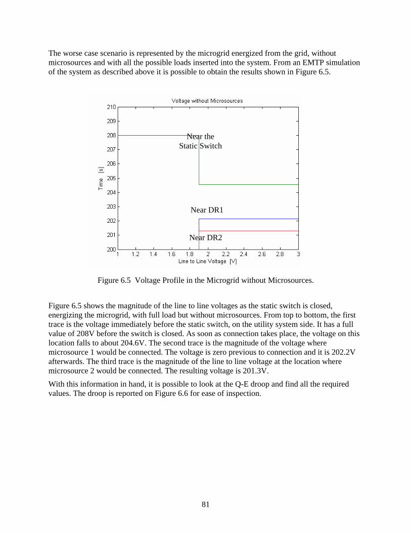
81

The worse case scenario is represented by the microgrid energized from the grid, without microsources and with all the possible loads inserted into the system. From an EMTP simulation of the system as described above it is possible to obtain the results shown in Figure 6.5.

Figure 6.5 Voltage Profile in the Microgrid without Microsources.

Figure 6.5 shows the magnitude of the line to line voltages as the static switch is closed, energizing the microgrid, with full load but without microsources. From top to bottom, the first trace is the voltage immediately before the static switch, on the utility system side. It has a full value of 208V before the switch is closed. As soon as connection takes place, the voltage on this location falls to about 204.6V. The second trace is the magnitude of the voltage where microsource 1 would be connected. The voltage is zero previous to connection and it is 202.2V afterwards. The third trace is the magnitude of the line to line voltage at the location where microsource 2 would be connected. The resulting voltage is 201.3V.

With this information in hand, it is possible to look at the Q-E droop and find all the required values. The droop is reported on Figure 6.6 for ease of inspection.

Near the Static Switch

Near DR1

Near DR2

82

Figure 6.6 Q versus E Droop.

For Microsource 1:

The total drop is (208-201.3) = 5.8V = 2 ΔE.

It means that ΔE = 2.9V, so the setpoint for the voltage is:

Ereq = 208-ΔE = 208-2.9 = 205.1 V

Qmax was already calculated as 11.25kVar, so the slope for this droop is:

V/kVar 2578.025.119.2

max

==Δ

=Q

EmQ

That is, the voltage is allowed to change of 0.2578 Volts for every kVar that is injected.

For Microsource 2:

The total drop is (208-202.2) = 6.7 V = 2 ΔE.

It means that ΔE = 3.35V , so the setpoint for the voltage is:

Ereq = 208-ΔE = 208-3.35 = 204.65 V

And the slope for the droop is:

V/kVar 2978.025.1135.3

max

==Δ

=Q

EmQ

That is, the voltage is allowed to change of 0.2978 Volts for every kVar that is injected.

EΔ

EΔ

oE

Q

maxQ

max Q −

InductiveRegion

CapacitiveRegion

reqE

83

The filtering is achieved by a low pass LC circuit. The capacitors are connected at delta. The values for the components are:

L = 1.2 mH

C = 30 μF

Table 6.4 summarizes all the data relevant to the microsources.

Table 6.4 Summary of Microsource Data.

6.3 Control Implementation Microsource control can be implemented with a limited number of measurements passed to a hardware block that creates the pulses for the gates of the power electronic devices inside the inverter. The hardware block consists of three distinct boards. The first board is responsible for conditioning the values of the measured quantities to voltage levels that allow the interface with the second board, the DSP. The DSP implements the control block, constantly comparing desired and measured quantities to generate the gate pulses. These pulses are then passed to the third board, that amplifies the low voltage pulse signals coming out from the DSP to the voltage level needed to operate the actual power electronic devices.

The control blocks are encoded in Assembly language and compiled with Metrowerks CodeWarrior software. The executable code is then passed to the program memory of the DSP board.

The Digital Signal Processor (DSP) is a versatile hardware device that uploads an executable code with the information on how to manipulate inputs to generate outputs. The DSP is the ideal environment to code the control of the microsource. The input of this board are the signals coming from the sensing devices and the outputs are the firing pulses that are sent to the gates of the power electronics inside the inverter.

The code is uploaded in the DSP memory through a connection with a computer, where the program is compiled to an executable format. It is possible to debug the code by executing it on the DSP and sending some of the internal variables to dedicated pins where it is possible to connect with oscilloscope probes. The sensing signals reach the board as analog signals and are converted into digital form to be processed inside the integrated circuit. It is also possible to debug the code by means of a special application called PCMaster, a program written by Motorola to support the code builders for their DSP products.

V rated [V]

S rated

[kVA]

P rated [kW]

Q rated [kVar]

m [rad/kW] Qm

[V/kVar]

X

[Ω]

L [mH]

C [μF]

MS 1 480 18.75 15.0 11.25 0.15

π 0.2578 1.88 1.2 30

MS 2 480 18.75 15.0 11.25 0.15

π 0.2978 1.88 1.2 30

84

The DSP is an integrated chip mounted on a board that handles several peripherals for interfacing with the external world. Figure 6.7 shows the block schematic highlighting these peripherals:

i) Analog to Digital Conversion (ADC) to import measurement from the outside world as a string of bits stored in a mapped data memory

ii) Crystal oscillator clock that generates the square wave pulses to operate the CPU inside the integrated circuit

iii) Parallel pins to allow the gate signals to be passed to the signal amplifying board

iv) Digital to Analog Conversion (DAC) that is very useful when debugging the control routine allowing output signals to be displayed on the oscilloscope

v) Parallel connection to connect to the computer card that sends the compiled code to be stored in the program memory of the integrated circuit

vi) Interrupt request controller to be able to set up priorities in hardware and software queues of tasks that are waiting to be processed by the DSP

vii) Timer controller that can be used to generate any triangle or square wave that may be needed

viii) Serial port to allow to exchange values from and to the board with the computer

Figure 6.7 DSP Peripherals.

The DSP is a Motorola DSP56F805EVM board. Internally, this board handles every signal as a 16 bit word, and uses the fractional integer Arithmetic Logic Unit (ALU), a mathematical processor that supports only two kind of operations between register values: sum and multiplication. The ALU can only represent and use numbers between -1 and 1, demanding extra care when coding the control blocks. Every variable will have to be rescaled so that its value will never exceed the absolute value of unity, not even during overshooting transients. This board

Integrated Circuit

IRQ ADC

Oscillator Clocks

Parallel Port Timer

Module

Parallel Pins

DAC

External Measurements

Executable from Computer

Oscilloscope Probe

Inverter Gates

DSP Board

Serial Port Debugging Utility

to Computer

85

works with an internal voltage level that can be ± 3.3 V or below and the internal oscillator can generate a frequencies up to 40MHz.

The basic concept in the DSP implementing architecture is that there is a main routine that is executed once every period of the switching frequency, 4kHz. This routine implements the control and the gate pulse generator. The Interrupt controller is the overseeing scheduling manager that decides when a program starts running according to a preassigned priority. Figure 6.8 shows the priority of the programs that are running inside the DSP.

Figure 6.8 Interrupt Routine Queue.

The lowest priority program is a No Operation (NOP) routine, substantially it is a main function with an empty body. The higher priority program returns control to the Interrupt controller after it is done. When the NOP routine ends, the Interrupt controller immediately starts it again: in this case the processor is kept in a stand-by, or busy-wait state. NOP has the lowest priority and can be interrupted at any time.

The Interrupt control will generate a request to run the control block operation and gate pulse generation routine four thousand times every second. In this way, gate pulses are generated at a frequency of 4kHz: this is the frequency at which switching positions change. As soon as the gate pulses calculation is active the NOP is frozen in time and the processor stores the position in memory from where it was interrupted. The Interrupt control will generate a request to run the NOP routine from exactly the point where it was stopped as soon as the routine that implements the control and pulse generation has returned from execution.

6.4 Gate Pulse Implementation with Space Vector Modulation This section describes the implementation based on the synthesization of a desired voltage vector. This operation results in a constant switching frequency and is typically referred in the literature as space vector modulation technique.

The inverter is represented in Figure 6.9: it is the simplest configuration possible, with one single level of six power electronic devices connected to a DC ideal voltage source. The gates of the silicon devices can be controlled independently, but there are some constraints that limit the choices on the possible positions. For instance, two switches on the same leg (such as 1g and

Interrupt Controller

Microsource Control and Gate Pulse

Generator

NOP

Higher Priority

86

4g ) can never be closed at the same time to avoid shorting the DC voltage source and one switch per leg must always be closed to provide a path for the AC current to flow.

Figure 6.9 Inverter Switch Topology.

This section shows the implementation of the space vector modulation technique to synthesize the voltage at the terminals of the inverter.

Figure 6.10 Voltage Control Blocks, Hardware with Space Vector Modulation.

Figure 6.10 summarizes the operations of the gate pulse generator as included in Figure 3.2. The gate pulse generator is composed of a cascade of two blocks. The first block is responsible for calculating the real and imaginary components of the voltage vector, starting from the magnitude and angle. From the Cartesian components of the voltages the conduction times for each of the tree voltages are calculated. Two of these voltages are active voltages, while the third one is the zero vector. The conduction times will determine how long each vector will need to be applied for ultimately synthesizing the requested voltage. The information on the conduction time is then passed to another block, that reads on a look up table the switching sequence to apply at the gate

1g 2g 3g

4g 5g 6g

+ DCVC

B

A

Inverter Terminals

Look Up Table

For Switching

Positions

1g

2g

3g

4g

5g

Gate Pulse Generator

Vδ

Calculation of

Conduction Times

otΔ

itΔ

jtΔ

V

6g

87

terminals to achieve each of the three vectors. The DSP has an internal read-only routine that interfaces with the external pins that carry the gate signals. Once it is fed with the conduction times and the switching sequence, this routine takes care of sending the proper gate signals at the right time.

The space vector modulation technique applies the time averaging concept by synthesizing a voltage vector as a rapid succession of discrete voltages so that their average over a small interval of time matches the desired voltage vector magnitude and phase. The inputs are the seven operation points of a six step inverter. Figure 6.11 shows the six vectors for the active positions and the zero vector.

Figure 6.11 Achievable Voltage Vectors and Desired Voltage Vector.

The goal is to synthesize a rotating vector by approximating its revolution as a succession of discrete positions. The position is updated every period of the switching frequency and gives a standstill value of the vector at that time,

ρVij as shown in Figure 6.11. The vector

ρVij , between

ρV1 and

ρV2 , can be achieved by taking the period of the switching frequency, Tz , and dividing it

into three quotas, each one representing the amount of time that one of the neighboring fixed voltages and the zero voltage is applied. The two neighboring vectors are from the six step operation as of Figure 6.11: for instance, with the placement of vector

ρVij as in this figure, then

1VViρρ

= and 2VV jρρ

= . Maintaining the more general nomenclature by calling ρVi and

ρVj these

two vectors, it is possible to write:

T t t t

V V t V t V tz o i j

ij z o o i i j j

= + +

= + +

Δ Δ Δ

Δ Δ Δρ ρ ρ ρ

T

From the equations above it is obvious that otΔ is the amount of time the zero vector is applied and ji t ,t ΔΔ are respectively the amount of times that vectors

ρVi and

ρVj are applied. The sum of

the three times intervals must equal the period of the switching frequency.

The three intervals of time are unknown, and the second equation is a complex constraint hiding two real equations, yielding the consistent set of three equations in three unknowns to obtain the conduction times. The calculation of times occurs every period Tz . The real coefficients of the

V1

ρV2

ρV3

ρV4

ρV5

ρV6

ρVo

ρVij

88

vector ρVij can be generated following the definition of vector theory that says that the real part

of a vector is the projection on the ‘x’ axis while the imaginary is the projection on the ‘y’ axis:

{ } { }{ }{ } )tsin(V)t(V

)tcos(V)t(V

)t(V j)t(V)t(V

req voreqij

req voreqij

ijijij

δ+ω=

δ+ω=

+=

ρ

ρ

ρρρ

Im

Re

ImRe

The requested voltage and angle can be obtained from the output quantities of the inverter.

The vectors from the six step operation (Figure 6.11) are reported here:

ρ ρ

ρ ρ

ρ ρ

V V e V V e

V V e V V e

V V e V V e

DCj

DCj

DCj

DCj

DCj

DCj

10

4

23

5

43

3

23

6

53

23

23

23

23

23

23

= =

= =

= =

* *

π

ππ

π π

These vectors are fixed and their real and imaginary part needs to be calculated only once. The coefficient 2/3 comes from the consideration that although the applied voltage equals VDC , the voltage across the phase 'a' from its terminals to the imaginary neutral point would only see 2/3 of the full voltage, as shown in Figure 6.12.

Figure 6.12 Voltage Partition on the Inverter Legs.

Achieving these voltages is only a matter of looking up the correct set of switches that have to be closed for each of the desired voltages. A lookup table (shown on Table 6.5) based on Figure 6.11 and on the six step voltage definition is created and reported below.

VDC A

B C

23

VDC

13

VDC

89

Table 6.5 Lookup Table for Switching Positions.

The fixed voltages from the six step operation are known and constant, Tz is determined by the switching frequency, while vector

ρVij is built starting from the controller's output signals. The

formulation of the space vector problem with all the variables expressed as real quantities that can be implemented on a DSP environment is:

{ } { } { } { }{ } { } { } { }{ } { }

{ }

Δ

ΔΔ

Δ Δ Δ

t TV V V V

V V V V

tT V tj V

Vt T t tj

j zi ij i ij

i j i j

iz ij j

i

o z i

=−

−

=−

= − −

Re Im Im Re

Re Im Im Re

Re Re

Re

ρ ρ ρ ρ

ρ ρ ρ ρ

ρ ρ

ρ

* *

* *

These equations need to be solved for every period of the switching frequency determining which voltage vectors need to be applied and for how long. Figure 6.13 shows the full diagram of the gate pulse generator that can be interfaced with the output control quantities:

Closed Switches

Leg A Leg B Leg C ρVo 1 2 3 ρV1 1 5 6 ρV2 1 5 6 ρV3 4 2 6 ρV4 4 2 3 ρV5 4 2 3 ρV6 1 5 3

90

Figure 6.13 Gate Pulse Generator Block for Space Vector Modulation.

This modulation technique guarantees a constant switching frequency because at every period the sequence of conducting times will be started anew. The rotating vector changes at every switching period as it rotates, but even if it was held constant, the switching sequence would still repeat voltage iV

ρ for time iT , jV

ρ for time jT and oV

ρ for time oT : that is the switches would not

be locked to a constant position forever.

Creation of Rotating

Vector

Calculation of

Conduction Times

Look-Up

Table for Gate Pulses

{ }ReρVij

{ }ImρVij

Gate Signals

61g >−

reqV

Vreqδ

Calculation of Neighboring

Six Step Voltages

ijVρ

ji V ,Vρρ

jio T,T ,T ΔΔΔ

91

Chapter 7. Microgrid Tests

There are two fundamental different circuits where the test is performed depending on the relative locations of the two units. These two circuits are the series and the parallel configurations. Figure 7.1(a) shows the series configuration, while Figure 7.1(b) shows the parallel configuration. Both configurations are achieved with the same hardware equipment, appropriately rearranged. Each of the five loads may be included or not in every particular experiment. To avoid confusion, every experiment will explicitly show the full circuit diagram used.

Figure 7.1 Series (a) and Parallel (b) Circuit Configurations.

Each of the two sources can adopt either unit power (P) control or feeder flow (F) control. There are a total of four possible control combinations for the two units: PP, FF, PF, and FP. The circuit with the series configuration will test all these cases, while the parallel configuration will only test FF and FP. This is no loss of generality. The case PF is symmetric to FP and adds no useful insight. The case with PP is non dependent on the location of the sources and the loads and will give the same exact results already obtained for the series configuration. In conclusion, these are the six groups of tests:

Series configuration:

Unit 1 controls P, Unit 2 controls P

Unit 1 controls F, Unit 2 controls F

Unit 1 controls F, Unit 2 controls P

Unit 1 controls P, Unit 2 controls F

Parallel Configuration

Unit 1 controls F, Unit 2 controls F

Utility System

1P

1F

2P

2F

1L 3L 4L 5L

4 wire 75yd

4 wire 25yd

2L

Utility System 1P

1F

2P

2F 1L

3L 4L4 wire 75yd

4 wire 25yd

2L

5L

(a)

(b)

92

Unit 1 controls F, Unit 2 controls P

Each test groups is configured as follows:

Import from grid:

− Unit 1 at 50% of its ratings, Unit 2 at 50% of its ratings – transfer to island

− Unit 1 at 10%, Unit 2 at 90% – transfer to island (i), usually Unit 2 reaches maximum output

− From this (i) island operating point, remove a load , this backs off the unit from maximum output

− Again, from (i) reduce setpoint of Unit 2, this backs off the unit from maximum output

− Unit 1 at 90%, Unit 2 at 10% – transfer to island, usually Unit 1 reaches maximum output

Export to grid:

− Unit 1 at 50% of its ratings, Unit 2 at 50% of its ratings – transfer to island

− Unit 1 at 10%, Unit 2 at 90% – transfer to island, usually Unit 1 reaches zero output

− Unit 1 at 90%, Unit 2 at 10% – transfer to island (e), usually Unit 2 reaches zero output

− From this (e) island operating point, insert a load , this backs off the unit from zero output

− Again, from (e) increase setpoint of Unit 2, this backs off the unit from zero output

Every group has five experiments while importing and five while exporting. When at least one of the units regulates feeder flow (all but the very first test group, series PP), then there are two added experiments when importing from the grid:

− Unit 1 at 10%, Unit 2 at 90% - the unit regulating F is switched to a wrong setpoint that will determine either max or zero power output.

− Unit 1 at 90%, Unit 2 at 10% - the same unit regulating F is switched to a wrong setpoint that will determine max (if before it was zero) or zero (if before it was max) output.

If both units are regulating F, then one unit is arbitrarily picked up to test the wrong setpoint feature.

In summary, in each test group the experiments will be carried in the order shown in Table 7.1.

93

Table 7.1 Summary of Experiments for Each Group of Tests.

7.1 Choice of Setpoints for the Series Configuration There are four possible control choices in the series configuration:

i) unit 1 controlling P, unit 2 controlling P

ii) unit 1 controlling F, unit 2 controlling F

iii) unit 1 controlling F, unit 2 controlling P

iv) unit 1 controlling P, unit 2 controlling F

For each choice (see Table 7.1), there is an experiment when unit 1 is at 10% of its output power, while unit 2 is at 90% of its output power and the system transfers to island. Figure 7.2 shows the series configuration with all the loads, highlighting the fact that the only event taking place is the transition to island. The system is importing from the grid.

Unit 1 Unit 2 (*) NOT there if both unit control unit output power, P

50% 50% Islanding

10% 90% Wrong Setpoint at One of the Units Controlling F (*)

10% 90% Islanding, to Operating Point (i)

10% 90% From Island, (i), Remove a Load

10% 90% From Island, (i), Reduce Setpoint of Unit at Maximum Power

90% 10% Wrong Setpoint at One of the Units Controlling F (*)

Import Power From the Grid

90% 10% Islanding

50% 50% Islanding

10% 90% Islanding

90% 10% Islanding, to Operating Point (e)

90% 10% From Island, (e), Insert a Load

Export Power From the Grid

90% 10% From Island, (e), Increase Setpoint of Unit at Zero Power

94

Figure 7.2 Series Configuration Diagram.

Maximum power corresponds to 0.8 pu in the source because of the DSP capability of handling only quantities that are in the –1,+1 interval. To leave room for overshoot, the value of P_max has been chosen to correspond to 0.8.

After the system transfers to island, unit 2 will be sitting at 100% of power (0.8 pu), while unit 1 will be sitting at 50% (since overall loading is 150%) of power (0.4 pu), in all of the four configurations. What really changes, is how they get there.

Figure 7.3 and Figure 7.4 show simulation results when P1 and P2 are controlled: both units ramp up their power output (P) at the unison. Overshoot at unit 2 is near 0.89 pu (110%).

Figure 7.5 and Figure 7.6 show that when F1 and F2 are controlled, then as P2 ramps, P1 actually backs off, after rising a little. This means that the resulting overshoot on P2 is about 1.04 pu (130%). This implies tripping of the units, since nearly above 0.9 pu is the threshold value for power, and besides, a value larger than 1.0 is also beyond the overflow value of the bit representation inside the DSP.

Figure 7.7 and Figure 7.8 show that when F1 and P2 are controlled, then an unacceptable overshoot also occurs. Figure 7.9 and Figure 7.10 show that when P1 and F2 are controlled, the overshoot is manageable again.

This implies that the choice of control configurations bears a consequence on the ratings of the inverters that need to be available, or the gains may need to be readjusted (when possible) to improve response. For this lab case, the above considerations implied that the test for 10% and 90% could not be carried under those cases that generated very large overshoots. To avoid tripping of the units, the setpoint corresponding to loading of respectively 30% and 70% for unit 1 and 2 have been chosen only for the cases with larger overshoot. This problem was only encountered during 10%, 90% setup, never during 90%, 10%, hence this latter configuration has never been changed. Also these problems are only encountered at high load levels (importing to grid). Therefore, during exporting no changes were necessary to 10%, 90% setup. Finally, no problems were encountered during the parallel configuration, so no changes had to be made there as well.

The Table 7.2 below summarizes the previous considerations.

Utility System

1P

1F

2P

2F

1L 3L 4L 5L

4 wire 75yd

4 wire 25yd

Event: Transfer to

Island

95

Table 7.2 Series Configuration Control Combinations. Importing from Grid.

Figure 7.3 Control of P1 and P2, Unit Power.

Control of Unit 1 Control of Unit 2 Overshoot on Unit 2 P P 0.89 pu ~ 110% F F 1.04 pu ~ 130% F P 1.04 pu ~ 130% P F 0.89 pu ~ 110%

96

Figure 7.4 Control of P1 and P2, Feeder Flow.

Figure 7.5 Control of F1 and F2, Unit Power.

97

Figure 7.6 Control of F1 and F2, Feeder Flow.

Figure 7.7 Control of F1 and P2, Unit Power.

98

Figure 7.8 Control of F1 and P2, Feeder Flow.

Figure 7.9 Control of P1 and F2, Unit Power.

99

Figure 7.10 Control of P1 and F2, Feeder Flow.

7.2 Grid Fluctuations The nominal grid frequency is 60Hz, but it has been measured to drift around it. Figure 7.11 shows two samples of the frequency, taken less than five minutes apart. One has a –0.04Hz deviation, while the other has a +0.06Hz deviation. This frequency deviation translates in the fact that the active power may not exactly match the request. Figure 7.12 shows that with a Δf=0.05Hz the corresponding variation of the power setpoint is 0.08 pu, or 10 % of the ratings. This justifies the fact that in some of the plots in grid connection, the values of the injected power is not exactly as demanded, but may be different, sometimes about 10% off.

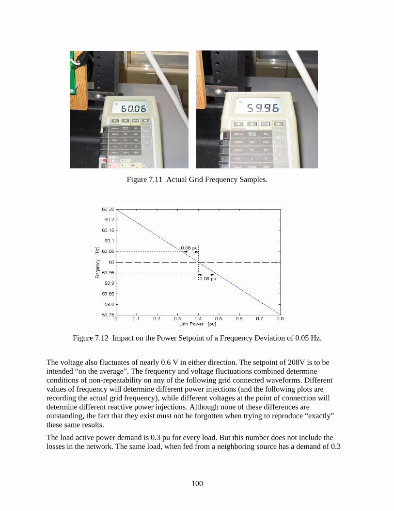
100

Figure 7.11 Actual Grid Frequency Samples.

Figure 7.12 Impact on the Power Setpoint of a Frequency Deviation of 0.05 Hz.

The voltage also fluctuates of nearly 0.6 V in either direction. The setpoint of 208V is to be intended “on the average”. The frequency and voltage fluctuations combined determine conditions of non-repeatability on any of the following grid connected waveforms. Different values of frequency will determine different power injections (and the following plots are recording the actual grid frequency), while different voltages at the point of connection will determine different reactive power injections. Although none of these differences are outstanding, the fact that they exist must not be forgotten when trying to reproduce “exactly” these same results.

The load active power demand is 0.3 pu for every load. But this number does not include the losses in the network. The same load, when fed from a neighboring source has a demand of 0.3

101

pu, but when it is fed from a remote source (or the grid) may demand as much as 0.31 or bigger, usually never above 0.32 pu. Three remote loads may show up as 0.95 pu, rather than 0.9 pu.

7.3 Series Configuration This configuration represents the classic radial distributed system: there is a single feeder with two sources in series and loads scattered: some of them are near each of the two sources, a load in an intermediate location between the sources. The overall length of cable between the sources is 100yds.

Figure 7.13 shows the general layout of the system with the series configuration.

Figure 7.13 Units in Series Configuration.

Utility System

1P

1F

2P

2F

1L 3L 4L 5L

4 wire 75yd

4 wire 25yd

2L

102

7.3.1 Unit 1 (P), Unit 2 (P), Import from Grid

Import From Grid, Setpoints are 50% and 50% of Unit Rating, Islanding Event shows Unit 1 and 2 meeting the load request after islanding.

Intermediate Bus (Load 3L ) Voltage, 200ms/div.

Series Configuration, Control of 1P and 2P

A – Grid B – Island

1P [pu] 0.4 = 50% 0.6 = 75%

2P [pu] 0.4 = 50% 0.6 = 75% Frequency

[Hz] 60.00 59.875

Load Level [pu] 1.2 = 150% 1.2 = 150%

Grid Flow [pu] 0.4 = 50% 0.0

Utility System

1P

1F

2P

2F

1L 3L 4L 5L

4 wire 75yd

4 wire 25yd

Event: Transfer to Island

103

Unit 1: P, Q, F, Frequency, Voltage Magnitude, Current Magnitude, 500ms/div.

Unit 2: P, Q, F, Frequency, Voltage Magnitude, Current Magnitude, 500ms/div.

104

Import From Grid, Setpoints are 10% and 90% of Unit Rating, Islanding Event shows Unit 2 reaching maximum output power after islanding.

Intermediate Bus (Load 3L ) Voltage, 200ms/div.

Series Configuration, Control of 1P and 2P

A – Grid B – Island

1P [pu] 0.08 = 10% 0.4 = 50%

2P [pu] 0.72 = 90% 0.8 = 100% Frequency

[Hz] 60.00 59.8

Load Level [pu] 1.2 = 150% 1.2 = 150%

Grid Flow [pu] 0.4 = 50% 0.0

Utility System

1P

1F

2P

2F

1L 3L 4L 5L

4 wire 75yd

4 wire 25yd

Event: Transfer to Island

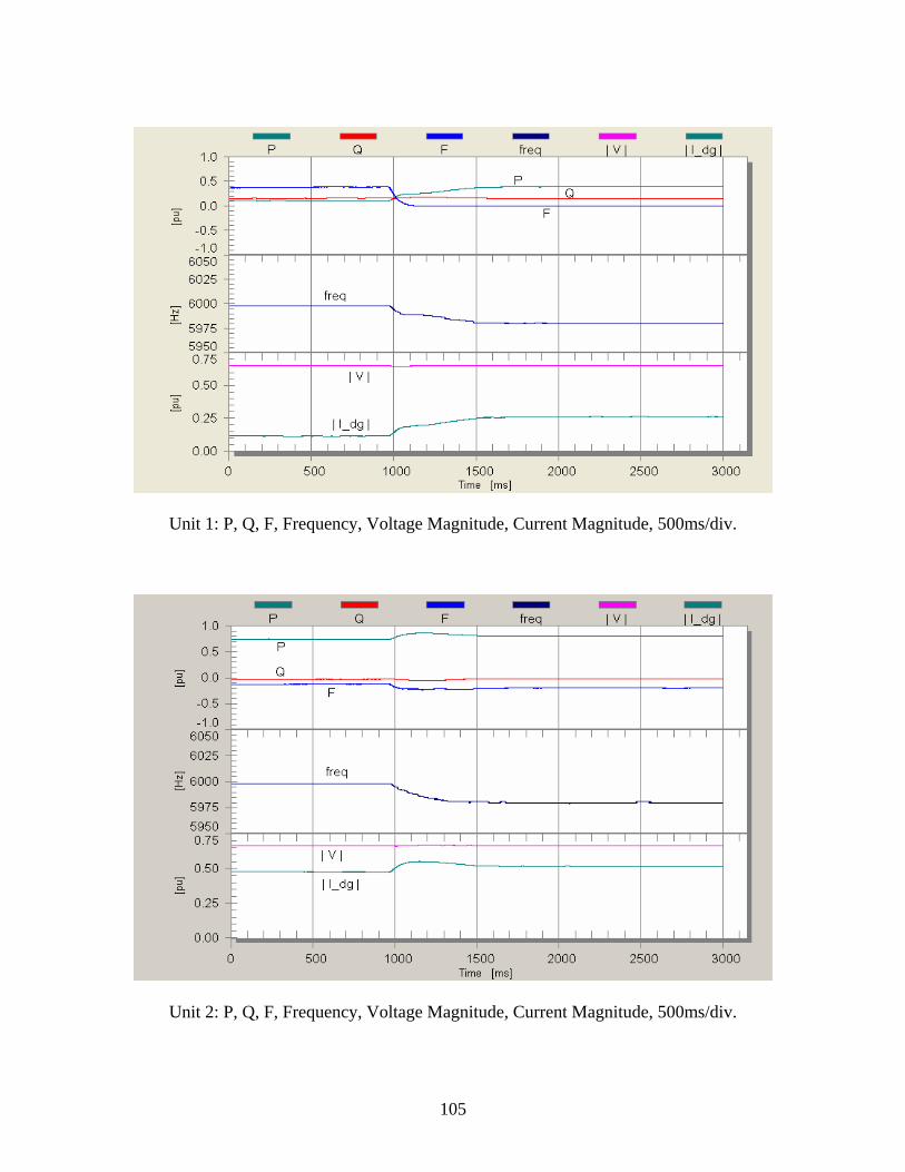
105

Unit 1: P, Q, F, Frequency, Voltage Magnitude, Current Magnitude, 500ms/div.

Unit 2: P, Q, F, Frequency, Voltage Magnitude, Current Magnitude, 500ms/div.

106

Island, Setpoints are 10% and 90% of Unit Rating, Load Removal Event shows Unit 2 backing off from maximum output power after a load is removed.

Intermediate Bus (Load 3L ) Voltage, 200ms/div.

Series Configuration, Control of 1P and 2P

A – 5L on B – 5L off

1P [pu] 0.4 = 50% 0.13 = 16%

2P [pu] 0.8 = 100% 0.77 = 96% Frequency

[Hz] 59.8 59.968

Load Level [pu] 1.2 = 150% 0.9 = 112%

Grid Flow [pu] 0.0 0.0

Utility System

1P

1F

2P

2F

1L 3L 4L 5L

4 wire 75yd

4 wire 25yd

Event: Load 5L Removal

107

Unit 1: P, Q, F, Frequency, Voltage Magnitude, Current Magnitude, 500ms/div.

Unit 2: P, Q, F, Frequency, Voltage Magnitude, Current Magnitude, 500ms/div.

108

Island, Setpoints are 10% and 90% of Unit Rating, Setpoint Change Event shows Unit 2 backing off from maximum output power after power setpoint of unit 2 has been reduced.

Intermediate Bus (Load 3L ) Voltage, 200ms/div.

Series Configuration, Control of 1P and 2P

A 2P =90% B 2P =50%

1P [pu] 0.4 = 50% 0.44 = 55%

2P [pu] 0.8 = 100% 0.76 = 95% Frequency

[Hz] 59.8 59.775

Load Level [pu] 1.2 = 150% 1.2 = 150%

Grid Flow [pu] 0.0 0.0

Utility System

1P

1F

2P

2F

1L 3L 4L 5L

4 wire 75yd

4 wire 25yd

Event: Setpoint 2P Change

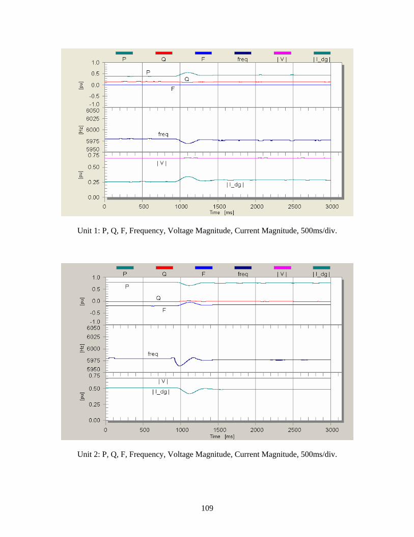
109

Unit 1: P, Q, F, Frequency, Voltage Magnitude, Current Magnitude, 500ms/div.

Unit 2: P, Q, F, Frequency, Voltage Magnitude, Current Magnitude, 500ms/div.

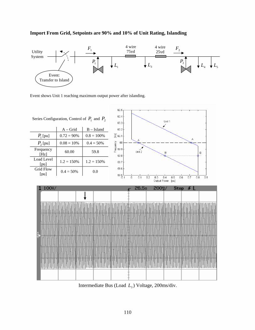
110

Import From Grid, Setpoints are 90% and 10% of Unit Rating, Islanding Event shows Unit 1 reaching maximum output power after islanding.

Intermediate Bus (Load 3L ) Voltage, 200ms/div.

Series Configuration, Control of 1P and 2P

A – Grid B – Island

1P [pu] 0.72 = 90% 0.8 = 100%

2P [pu] 0.08 = 10% 0.4 = 50% Frequency

[Hz] 60.00 59.8

Load Level [pu] 1.2 = 150% 1.2 = 150%

Grid Flow [pu] 0.4 = 50% 0.0

Utility System

1P

1F

2P

2F

1L 3L 4L 5L

4 wire 75yd

4 wire 25yd

Event: Transfer to Island

111

Unit 1: P, Q, F, Frequency, Voltage Magnitude, Current Magnitude, 500ms/div.

Unit 2: P, Q, F, Frequency, Voltage Magnitude, Current Magnitude, 500ms/div.

112

7.3.2 Unit 1 (P), Unit 2 (P), Export to Grid

Export to Grid, Setpoints are 50% and 50% of Unit Rating, Islanding Event shows Unit 1 and 2 meeting the load request after islanding.

Intermediate Bus (Load 3L ) Voltage, 200ms/div.

Series Configuration, Control of 1P and 2P A – Grid B – Island

1P [pu] 0.4 = 50% 0.3 = 37%

2P [pu] 0.4 = 50% 0.3 = 37% Frequency

[Hz] 60.00 60.062

Load Level [pu] 0.6 = 75% 0.6 = 75%

Grid Flow [pu] -0.2 = -25% 0.0

Utility System

1P

1F

2P

2F

3L 4L

4 wire 75yd

4 wire 25yd

Event: Transfer to Island

113

Unit 1: P, Q, F, Frequency, Voltage Magnitude, Current Magnitude, 500ms/div.

Unit 2: P, Q, F, Frequency, Voltage Magnitude, Current Magnitude, 500ms/div.

114

Export to Grid, Setpoints are 10% and 90% of Unit Rating, Islanding Event shows Unit 1 reaching zero output power after islanding.

Intermediate Bus (Load 3L ) Voltage, 200ms/div.

Series Configuration, Control of 1P and 2P

A – Grid B – Island

1P [pu] 0.08 = 10% 0.0

2P [pu] 0.72 = 90% 0.6 = 75% Frequency

[Hz] 60.00 60.075

Load Level [pu] 0.6 = 75% 0.6 = 75%

Grid Flow [pu] -0.2 = -25% 0.0

Utility System

1P

1F

2P

2F

3L 4L

4 wire 75yd

4 wire 25yd

Event: Transfer to Island

115

Unit 1: P, Q, F, Frequency, Voltage Magnitude, Current Magnitude, 500ms/div.

Unit 2: P, Q, F, Frequency, Voltage Magnitude, Current Magnitude, 500ms/div.

116

Island, Setpoints are 10% and 90% of Unit Rating, Load Insertion Event shows Unit 2 backing off from zero output power after a load is inserted.

Intermediate Bus (Load 3L ) Voltage, 200ms/div.

Series Configuration, Control of 1P and 2P

A – 5L off B – 5L on

1P [pu] 0.0 0.13 = 16%

2P [pu] 0.6 = 75% 0.77 = 96% Frequency

[Hz] 60.075 59.968

Load Level [pu] 0.6 = 75% 0.9 = 112%

Grid Flow [pu] 0.0 0.0

Utility System

1P

1F

2P

2F

3L 4L 5L

4 wire 75yd

4 wire 25yd

Event: Load 5L Insertion

117

Unit 1: P, Q, F, Frequency, Voltage Magnitude, Current Magnitude, 500ms/div.

Unit 2: P, Q, F, Frequency, Voltage Magnitude, Current Magnitude, 500ms/div.

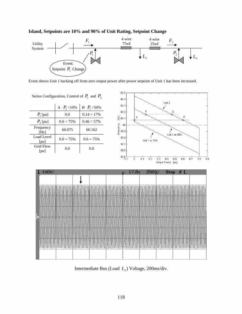
118

Island, Setpoints are 10% and 90% of Unit Rating, Setpoint Change

Event shows Unit 1 backing off from zero output power after power setpoint of Unit 1 has been increased.

Intermediate Bus (Load 3L ) Voltage, 200ms/div.

Series Configuration, Control of 1P and 2P

A 1P =10% B 1P =50%

1P [pu] 0.0 0.14 = 17%

2P [pu] 0.6 = 75% 0.46 = 57% Frequency

[Hz] 60.075 60.162

Load Level [pu] 0.6 = 75% 0.6 = 75%

Grid Flow [pu] 0.0 0.0

Utility System

1P

1F

2P

2F

3L 4L

4 wire 75yd

4 wire 25yd

Event: Setpoint 1P Change

119

Unit 1: P, Q, F, Frequency, Voltage Magnitude, Current Magnitude, 500ms/div.

Unit 2: P, Q, F, Frequency, Voltage Magnitude, Current Magnitude, 500ms/div.

120

Export to Grid, Setpoints are 90% and 10% of Unit Rating, Islanding

Event shows Unit 2 reaching zero output power after islanding.

Intermediate Bus (Load 3L ) Voltage, 200ms/div.

Series Configuration, Control of 1P and 2P

A – Grid B – Island

1P [pu] 0.72 = 90% 0.6 = 75%

2P [pu] 0.08 = 10% 0.0 Frequency

[Hz] 60.00 60.075

Load Level [pu] 0.6 = 75% 0.6 = 75%

Grid Flow [pu] -0.2 = -25% 0.0

Utility System

1P

1F

2P

2F

3L 4L

4 wire 75yd

4 wire 25yd

Event: Transfer to Island

121

Unit 1: P, Q, F, Frequency, Voltage Magnitude, Current Magnitude, 500ms/div.

Unit 2: P, Q, F, Frequency, Voltage Magnitude, Current Magnitude, 500ms/div.

122

7.3.3 Unit 1 (F), Unit 2 (F), Import from Grid

Import From Grid, Setpoints are 50% and 50% of Unit Rating, Islanding Event shows Unit 1 and 2 meeting the load request after islanding.

Intermediate Bus (Load 3L ) Voltage, 200ms/div.

Series Configuration, Control of 1F and 2F

A – Grid B – Island

1P [pu] 0.4 = 50% 0.4 = 50%

2P [pu] 0.4 = 50% 0.8 = 100% Frequency

[Hz] 60.00 59.75

Load Level [pu] 1.2 = 150% 1.2 = 150%

Grid Flow [pu] 0.4 = 50% 0.0

Utility System

1P

1F

2P

2F

1L 3L 4L 5L

4 wire 75yd

4 wire 25yd

Event: Transfer to Island

123

Unit 1: P, Q, F, Frequency, Voltage Magnitude, Current Magnitude, 500ms/div.

Unit 2: P, Q, F, Frequency, Voltage Magnitude, Current Magnitude, 500ms/div.

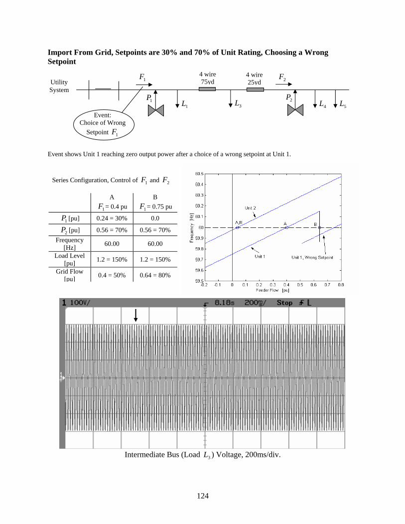
124

Import From Grid, Setpoints are 30% and 70% of Unit Rating, Choosing a Wrong Setpoint

Event shows Unit 1 reaching zero output power after a choice of a wrong setpoint at Unit 1.

Intermediate Bus (Load 3L ) Voltage, 200ms/div.

Series Configuration, Control of 1F and 2F

A

1F = 0.4 pu B

1F = 0.75 pu

1P [pu] 0.24 = 30% 0.0

2P [pu] 0.56 = 70% 0.56 = 70% Frequency

[Hz] 60.00 60.00

Load Level [pu] 1.2 = 150% 1.2 = 150%

Grid Flow [pu] 0.4 = 50% 0.64 = 80%

Utility System

1P

1F

2P

2F

1L 3L 4L 5L

4 wire 75yd

4 wire 25yd

Event: Choice of Wrong

Setpoint 1F

125

Unit 1: P, Q, F, Frequency, Voltage Magnitude, Current Magnitude, 500ms/div.

Unit 2: P, Q, F, Frequency, Voltage Magnitude, Current Magnitude, 500ms/div.

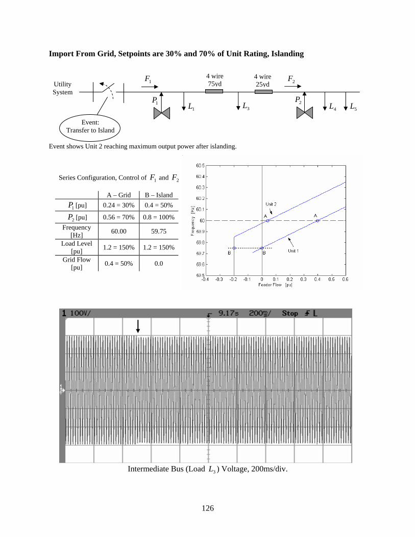
126

Import From Grid, Setpoints are 30% and 70% of Unit Rating, Islanding Event shows Unit 2 reaching maximum output power after islanding.

Intermediate Bus (Load 3L ) Voltage, 200ms/div.

Series Configuration, Control of 1F and 2F

A – Grid B – Island

1P [pu] 0.24 = 30% 0.4 = 50%

2P [pu] 0.56 = 70% 0.8 = 100% Frequency

[Hz] 60.00 59.75

Load Level [pu] 1.2 = 150% 1.2 = 150%

Grid Flow [pu] 0.4 = 50% 0.0

Utility System

1P

1F

2P

2F

1L 3L 4L 5L

4 wire 75yd

4 wire 25yd

Event: Transfer to Island

127

Unit 1: P, Q, F, Frequency, Voltage Magnitude, Current Magnitude, 500ms/div.

Unit 2: P, Q, F, Frequency, Voltage Magnitude, Current Magnitude, 500ms/div.

128

Island, Setpoints are 30% and 70% of Unit Rating, Load Removal Event shows Unit 2 backing off from maximum output power after a load is removed.

Intermediate Bus (Load 3L ) Voltage, 200ms/div.

Series Configuration, Control of 1F and 2F

A – 5L on B – 5L off

1P [pu] 0.4 = 50% 0.24 = 30%

2P [pu] 0.8 = 100% 0.66 = 82% Frequency

[Hz] 59.75 59.75

Load Level [pu] 1.2 = 150% 0.9 = 112%

Grid Flow [pu] 0.0 0.0

Utility System

1P

1F

2P

2F

1L 3L 4L 5L

4 wire 75yd

4 wire 25yd

Event: Load 5L Removal

129

Unit 1: P, Q, F, Frequency, Voltage Magnitude, Current Magnitude, 500ms/div.

Unit 2: P, Q, F, Frequency, Voltage Magnitude, Current Magnitude, 500ms/div.

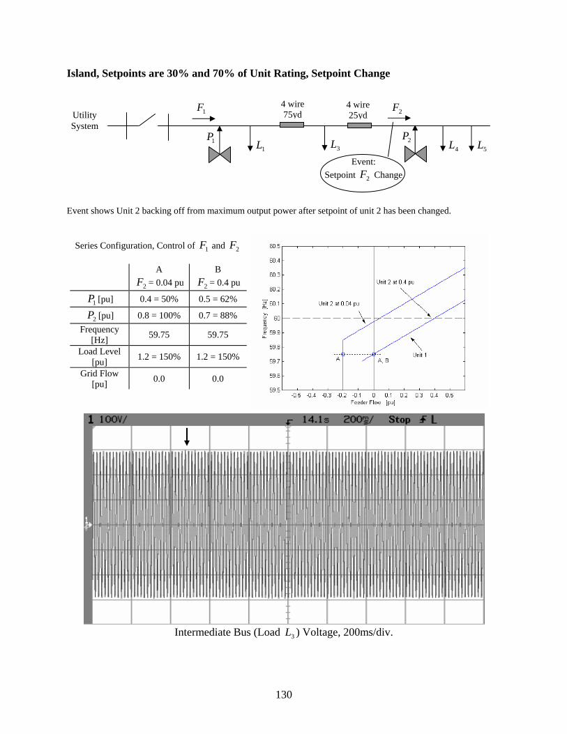
130

Island, Setpoints are 30% and 70% of Unit Rating, Setpoint Change

Event shows Unit 2 backing off from maximum output power after setpoint of unit 2 has been changed.

Intermediate Bus (Load 3L ) Voltage, 200ms/div.

Series Configuration, Control of 1F and 2F

A

2F = 0.04 pu B

2F = 0.4 pu

1P [pu] 0.4 = 50% 0.5 = 62%

2P [pu] 0.8 = 100% 0.7 = 88% Frequency

[Hz] 59.75 59.75

Load Level [pu] 1.2 = 150% 1.2 = 150%

Grid Flow [pu] 0.0 0.0

Utility System

1P

1F

2P

2F

1L 3L 4L 5L

4 wire 75yd

4 wire 25yd

Event: Setpoint 2F Change

131

Unit 1: P, Q, F, Frequency, Voltage Magnitude, Current Magnitude, 500ms/div.

Unit 2: P, Q, F, Frequency, Voltage Magnitude, Current Magnitude, 500ms/div.

132

Import From Grid, Setpoints are 90% and 10% of Unit Rating, Choosing a Wrong Setpoint

Event shows Unit 1 reaching maximum output power after a choice of a wrong setpoint at Unit 1.

Intermediate Bus (Load 3L ) Voltage, 200ms/div.

Series Configuration, Control of 1F and 2F

A

1F = 0.4 pu B

1F = 0.2 pu

1P [pu] 0.72 = 90% 0.8 = 100%

2P [pu] 0.08 = 10% 0.08 = 10% Frequency

[Hz] 60.00 60.00

Load Level [pu] 1.2 = 150% 1.2 = 150%

Grid Flow [pu] 0.4 = 50% 0.32 = 40%

Utility System

1P

1F

2P

2F

1L 3L 4L 5L

4 wire 75yd

4 wire 25yd

Event: Choice of Wrong

Setpoint 1F

133

Unit 1: P, Q, F, Frequency, Voltage Magnitude, Current Magnitude, 500ms/div.

Unit 2: P, Q, F, Frequency, Voltage Magnitude, Current Magnitude, 500ms/div.

134

Import From Grid, Setpoints are 90% and 10% of Unit Rating, Islanding Event shows Unit 1 reaching maximum output power after islanding.

Intermediate Bus (Load 3L ) Voltage, 200ms/div.

Series Configuration, Control of 1F and 2F

A – Grid B – Island

1P [pu] 0.72 = 90% 0.72 = 90%

2P [pu] 0.08 = 10% 0.48 = 60% Frequency

[Hz] 60.00 59.75

Load Level [pu] 1.2 = 150% 1.2 = 150%

Grid Flow [pu] 0.4 = 50% 0.0

Utility System

1P

1F

2P

2F

1L 3L 4L 5L

4 wire 75yd

4 wire 25yd

Event: Transfer to Island

135

Unit 1: P, Q, F, Frequency, Voltage Magnitude, Current Magnitude, 500ms/div.

Unit 2: P, Q, F, Frequency, Voltage Magnitude, Current Magnitude, 500ms/div.

136

7.3.4 Unit 1 (F), Unit 2 (F), Export to Grid

Export to Grid, Setpoints are 50% and 50% of Unit Rating, Islanding Event shows Unit 1 and 2 meeting the load request after islanding.

Intermediate Bus (Load 3L ) Voltage, 200ms/div.

Series Configuration, Control of 1F and 2F A – Grid B – Island

1P [pu] 0.4 = 50% 0.4 = 50%

2P [pu] 0.4 = 50% 0.2 = 25% Frequency

[Hz] 60.00 60.125

Load Level [pu] 0.6 = 75% 0.6 = 75%

Grid Flow [pu] -0.2 = -25% 0.0

Utility System

1P

1F

2P

2F

3L 4L

4 wire 75yd

4 wire 25yd

Event: Transfer to Island

137

Unit 1: P, Q, F, Frequency, Voltage Magnitude, Current Magnitude, 500ms/div.

Unit 2: P, Q, F, Frequency, Voltage Magnitude, Current Magnitude, 500ms/div.

138

Export to Grid, Setpoints are 10% and 90% of Unit Rating, Islanding Event shows feeder flow of Unit 1 going to zero after islanding.

Intermediate Bus (Load 3L ) Voltage, 200ms/div.

Series Configuration, Control of 1F and 2F

A – Grid B – Island

1P [pu] 0.08 = 10% 0.08 = 10%

2P [pu] 0.72 = 90% 0.52 = 65% Frequency

[Hz] 60.00 60.125

Load Level [pu] 0.6 = 75% 0.6 = 75%

Grid Flow [pu] -0.2 = -25% 0.0

Utility System

1P

1F

2P

2F

3L 4L

4 wire 75yd

4 wire 25yd

Event: Transfer to Island

139

Unit 1: P, Q, F, Frequency, Voltage Magnitude, Current Magnitude, 500ms/div.

Unit 2: P, Q, F, Frequency, Voltage Magnitude, Current Magnitude, 500ms/div.

140

Export to Grid, Setpoints are 90% and 10% of Unit Rating, Islanding

Event shows Unit 2 reaching zero output power after islanding.

Intermediate Bus (Load 3L ) Voltage, 200ms/div.

Series Configuration, Control of 1F and 2F

A – Grid B – Island

1P [pu] 0.72 = 90% 0.6 = 75%

2P [pu] 0.08 = 10% 0.0 Frequency

[Hz] 60.00 60.125

Load Level [pu] 0.6 = 75% 0.6 = 75%

Grid Flow [pu] -0.2 = -25% 0.0

Utility System

1P

1F

2P

2F

3L 4L

4 wire 75yd

4 wire 25yd

Event: Transfer to Island

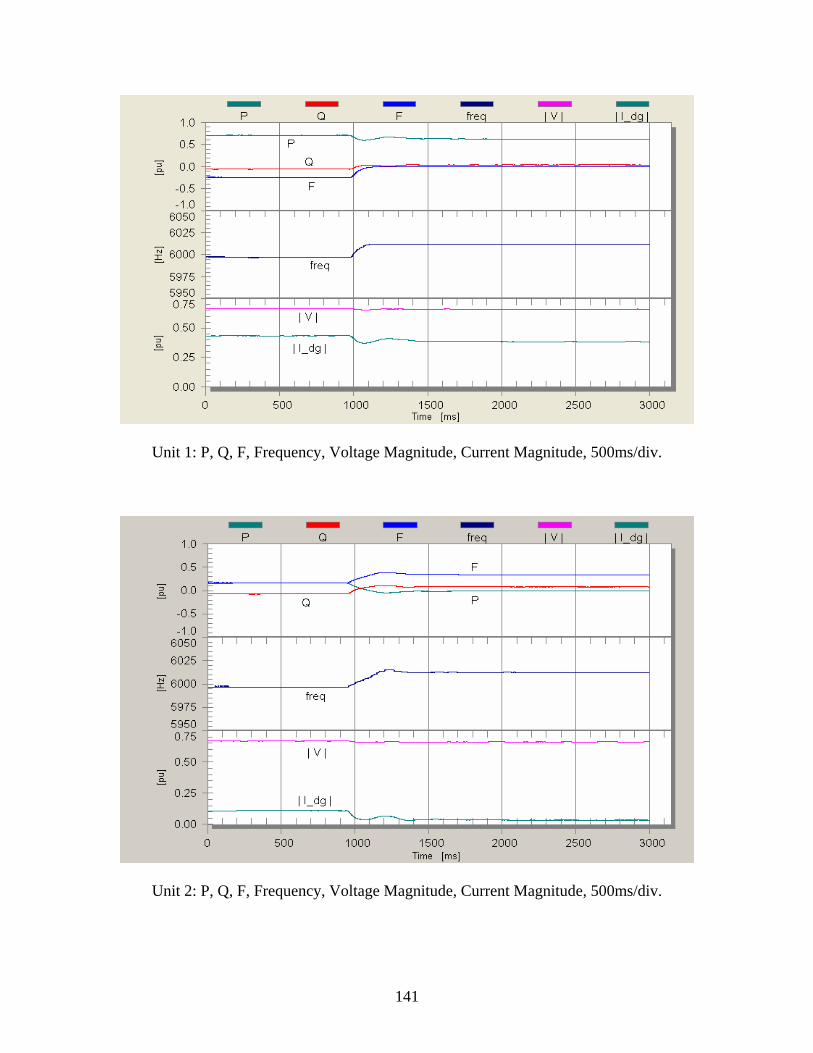
141

Unit 1: P, Q, F, Frequency, Voltage Magnitude, Current Magnitude, 500ms/div.

Unit 2: P, Q, F, Frequency, Voltage Magnitude, Current Magnitude, 500ms/div.

142

Island, Setpoints are 90% and 10% of Unit Rating, Load Insertion Event shows Unit 2 backing off from zero output power after a load is inserted.

Intermediate Bus (Load 3L ) Voltage, 200ms/div.

Series Configuration, Control of 1F and 2F

A – 5L off B – 5L on

1P [pu] 0.6 = 75% 0.72 = 90%

2P [pu] 0.0 0.18 = 22% Frequency

[Hz] 60.125 60.125

Load Level [pu] 0.6 = 75% 0.9 = 112%

Grid Flow [pu] 0.0 0.0

Utility System

1P

1F

2P

2F

3L 4L 5L

4 wire 75yd

4 wire 25yd

Event: Load 5L Insertion

143

Unit 1: P, Q, F, Frequency, Voltage Magnitude, Current Magnitude, 500ms/div.

Unit 2: P, Q, F, Frequency, Voltage Magnitude, Current Magnitude, 500ms/div.

144

Island, Setpoints are 90% and 10% of Unit Rating, Setpoint Change

Event shows Unit 2 backing off from zero output power after feeder flow setpoint of Unit 2 has been changed.

Intermediate Bus (Load 3L ) Voltage, 200ms/div.

Series Configuration, Control of 1F and 2F

A

2F = 0.2 pu B

2F = 0.0 pu

1P [pu] 0.6 = 75% 0.5 = 63%

2P [pu] 0.0 0.1 = 12% Frequency

[Hz] 60.125 60.125

Load Level [pu] 0.6 = 75% 0.6 = 75%

Grid Flow [pu] 0.0 0.0

Utility System

1P

1F

2P

2F

3L 4L

4 wire 75yd

4 wire 25yd

Event: Setpoint 2F Change

145

Unit 1: P, Q, F, Frequency, Voltage Magnitude, Current Magnitude, 500ms/div.

Unit 2: P, Q, F, Frequency, Voltage Magnitude, Current Magnitude, 500ms/div.

146

7.3.5 Unit 1 (F), Unit 2 (P), Import from Grid

Import From Grid, Setpoints are 50% and 50% of Unit Rating, Islanding Event shows Unit 1 and 2 meeting the load request after islanding.

Intermediate Bus (Load 3L ) Voltage, 200ms/div.

Series Configuration, Control of 1F and 2P

A – Grid B – Island

1P [pu] 0.4 = 50% 0.4 = 50%

2P [pu] 0.4 = 50% 0.8 = 100% Frequency

[Hz] 60.00 59.75

Load Level [pu] 1.2 = 150% 1.2 = 150%

Grid Flow [pu] 0.4 = 50% 0.0

Utility System

1P

1F

2P

2F

1L 3L 4L 5L

4 wire 75yd

4 wire 25yd

Event: Transfer to Island

147

Unit 1: P, Q, F, Frequency, Voltage Magnitude, Current Magnitude, 500ms/div.

Unit 2: P, Q, F, Frequency, Voltage Magnitude, Current Magnitude, 500ms/div.

148

Import From Grid, Setpoints are 30% and 70% of Unit Rating, Choosing a Wrong Setpoint

Event shows Unit 1 reaching zero output power after a choice of a wrong setpoint at Unit 1.

Intermediate Bus (Load 3L ) Voltage, 200ms/div.

Series Configuration, Control of 1F and 2P

A

1F = 0.4 pu B

1F = 0.75 pu

1P [pu] 0.24 = 30% 0.0

2P [pu] 0.56 = 70% 0.56 = 70% Frequency

[Hz] 60.00 60.00

Load Level [pu] 1.2 = 150% 1.2 = 150%

Grid Flow [pu] 0.4 = 50% 0.64 = 80%

Utility System

1P

1F

2P

2F

1L 3L 4L 5L

4 wire 75yd

4 wire 25yd

Event: Choice of Wrong

Setpoint 1F

149

Unit 1: P, Q, F, Frequency, Voltage Magnitude, Current Magnitude, 500ms/div.

Unit 2: P, Q, F, Frequency, Voltage Magnitude, Current Magnitude, 500ms/div.

150

Import From Grid, Setpoints are 30% and 70% of Unit Rating, Islanding Event shows Unit 2 reaching maximum output power after islanding.

Intermediate Bus (Load 3L ) Voltage, 200ms/div.

Series Configuration, Control of 1F and 2P

A – Grid B – Island

1P [pu] 0.24 = 30% 0.4 = 50%

2P [pu] 0.56 = 70% 0.8 = 100% Frequency

[Hz] 60.00 59.75

Load Level [pu] 1.2 = 150% 1.2 = 150%

Grid Flow [pu] 0.4 = 50% 0.0

Utility System

1P

1F

2P

2F

1L 3L 4L 5L

4 wire 75yd

4 wire 25yd

Event: Transfer to Island

151

Unit 1: P, Q, F, Frequency, Voltage Magnitude, Current Magnitude, 500ms/div.

Unit 2: P, Q, F, Frequency, Voltage Magnitude, Current Magnitude, 500ms/div.

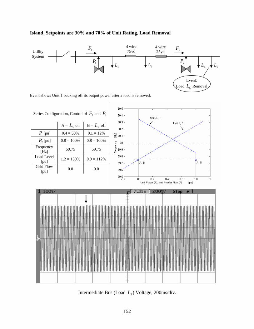
152

Island, Setpoints are 30% and 70% of Unit Rating, Load Removal Event shows Unit 1 backing off its output power after a load is removed.

Intermediate Bus (Load 3L ) Voltage, 200ms/div.

Series Configuration, Control of 1F and 2P

A – 5L on B – 5L off

1P [pu] 0.4 = 50% 0.1 = 12%

2P [pu] 0.8 = 100% 0.8 = 100% Frequency

[Hz] 59.75 59.75

Load Level [pu] 1.2 = 150% 0.9 = 112%

Grid Flow [pu] 0.0 0.0

Utility System

1P

1F

2P

2F

1L 3L 4L 5L

4 wire 75yd

4 wire 25yd

Event: Load 5L Removal

153

Unit 1: P, Q, F, Frequency, Voltage Magnitude, Current Magnitude, 500ms/div.

Unit 2: P, Q, F, Frequency, Voltage Magnitude, Current Magnitude, 500ms/div.

154

Island, Setpoints are 30% and 70% of Unit Rating, Setpoint Change

Event shows transients after power setpoint of Unit 2 has been reduced.

Intermediate Bus (Load 3L ) Voltage, 200ms/div.

Series Configuration, Control of 1F and 2P

A

2P = 0.56 pu B

2P = 0.4 pu

1P [pu] 0.4 = 50% 0.4 = 50%

2P [pu] 0.8 = 100% 0.8 = 100% Frequency

[Hz] 59.75 59.75

Load Level [pu] 1.2 = 150% 1.2 = 150%

Grid Flow [pu] 0.0 0.0

Utility System

1P

1F

2P

2F

1L 3L 4L 5L

4 wire 75yd

4 wire 25yd

Event: Setpoint 2P Change

155

Unit 1: P, Q, F, Frequency, Voltage Magnitude, Current Magnitude, 500ms/div.

Unit 2: P, Q, F, Frequency, Voltage Magnitude, Current Magnitude, 500ms/div.

156

Import From Grid, Setpoints are 90% and 10% of Unit Rating, Choosing a Wrong Setpoint

Event shows Unit 1 reaching maximum output power after a choice of a wrong setpoint at Unit 1.

Intermediate Bus (Load 3L ) Voltage, 200ms/div.

Series Configuration, Control of 1F and 2P

A

1F = 0.4 pu B

1F = 0.2 pu

1P [pu] 0.72 = 90% 0.8 = 100%

2P [pu] 0.08 = 10% 0.08 = 10% Frequency

[Hz] 60.00 60.00

Load Level [pu] 1.2 = 150% 1.2 = 150%

Grid Flow [pu] 0.4 = 50% 0.32 = 40%

Utility System

1P

1F

2P

2F

1L 3L 4L 5L

4 wire 75yd

4 wire 25yd

Event: Choice of Wrong

Setpoint 1F

157

Unit 1: P, Q, F, Frequency, Voltage Magnitude, Current Magnitude, 500ms/div.

Unit 2: P, Q, F, Frequency, Voltage Magnitude, Current Magnitude, 500ms/div.

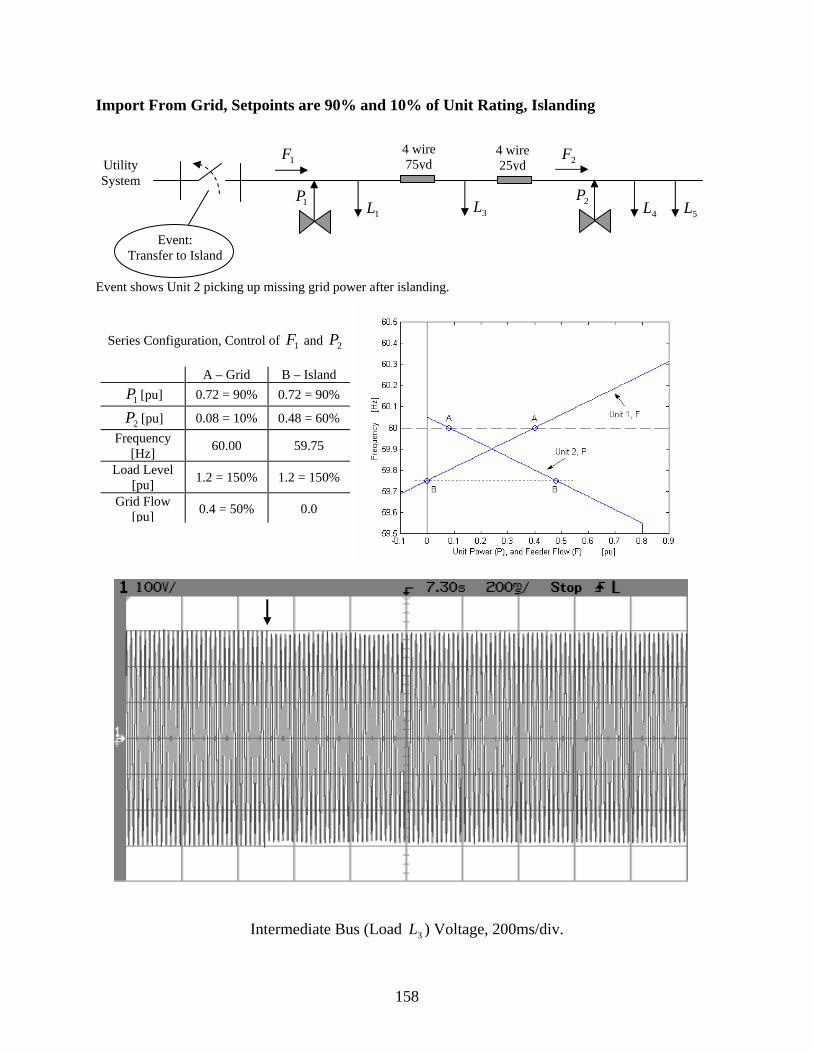
158

Import From Grid, Setpoints are 90% and 10% of Unit Rating, Islanding Event shows Unit 2 picking up missing grid power after islanding.

Intermediate Bus (Load 3L ) Voltage, 200ms/div.

Series Configuration, Control of 1F and 2P

A – Grid B – Island

1P [pu] 0.72 = 90% 0.72 = 90%

2P [pu] 0.08 = 10% 0.48 = 60% Frequency

[Hz] 60.00 59.75

Load Level [pu] 1.2 = 150% 1.2 = 150%

Grid Flow [pu] 0.4 = 50% 0.0

Utility System

1P

1F

2P

2F

1L 3L 4L 5L

4 wire 75yd

4 wire 25yd

Event: Transfer to Island

159

Unit 1: P, Q, F, Frequency, Voltage Magnitude, Current Magnitude, 500ms/div.

Unit 2: P, Q, F, Frequency, Voltage Magnitude, Current Magnitude, 500ms/div.

160

7.3.6 Unit 1 (F), Unit 2 (P), Export to Grid

Export to Grid, Setpoints are 50% and 50% of Unit Rating, Islanding Event shows Unit 1 and 2 meeting the load request after islanding.

Intermediate Bus (Load 3L ) Voltage, 200ms/div.

Series Configuration, Control of 1F and 2P A – Grid B – Island

1P [pu] 0.4 = 50% 0.4 = 50%

2P [pu] 0.4 = 50% 0.2 = 25% Frequency

[Hz] 60.00 60.125

Load Level [pu] 0.6 = 75% 0.6 = 75%

Grid Flow [pu] -0.2 = -25% 0.0

Utility System

1P

1F

2P

2F

3L 4L

4 wire 75yd

4 wire 25yd

Event: Transfer to Island

161

Unit 1: P, Q, F, Frequency, Voltage Magnitude, Current Magnitude, 500ms/div.

Unit 2: P, Q, F, Frequency, Voltage Magnitude, Current Magnitude, 500ms/div.

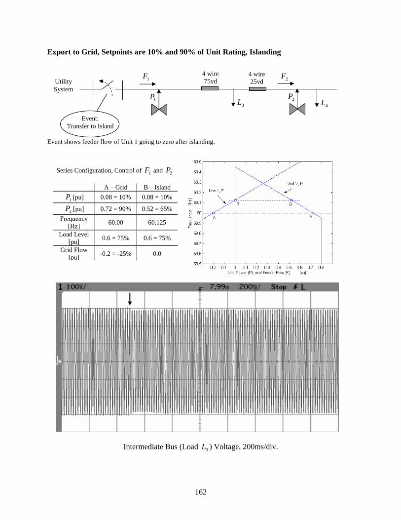
162

Export to Grid, Setpoints are 10% and 90% of Unit Rating, Islanding Event shows feeder flow of Unit 1 going to zero after islanding.

Intermediate Bus (Load 3L ) Voltage, 200ms/div.

Series Configuration, Control of 1F and 2P

A – Grid B – Island

1P [pu] 0.08 = 10% 0.08 = 10%

2P [pu] 0.72 = 90% 0.52 = 65% Frequency

[Hz] 60.00 60.125

Load Level [pu] 0.6 = 75% 0.6 = 75%

Grid Flow [pu] -0.2 = -25% 0.0

Utility System

1P

1F

2P

2F

3L 4L

4 wire 75yd

4 wire 25yd

Event: Transfer to Island

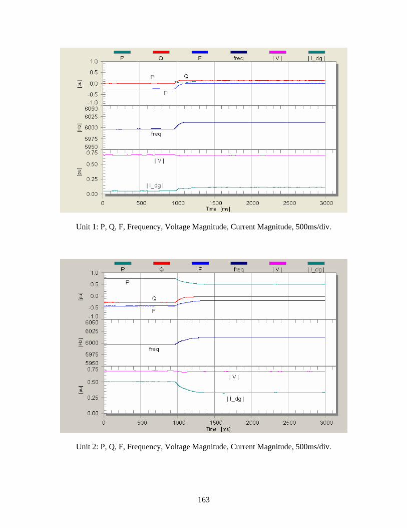
163

Unit 1: P, Q, F, Frequency, Voltage Magnitude, Current Magnitude, 500ms/div.

Unit 2: P, Q, F, Frequency, Voltage Magnitude, Current Magnitude, 500ms/div.

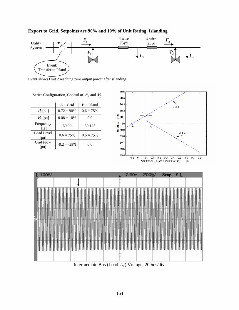
164

Export to Grid, Setpoints are 90% and 10% of Unit Rating, Islanding

Event shows Unit 2 reaching zero output power after islanding.

Intermediate Bus (Load 3L ) Voltage, 200ms/div.

Series Configuration, Control of 1F and 2P

A – Grid B – Island

1P [pu] 0.72 = 90% 0.6 = 75%

2P [pu] 0.08 = 10% 0.0 Frequency

[Hz] 60.00 60.125

Load Level [pu] 0.6 = 75% 0.6 = 75%

Grid Flow [pu] -0.2 = -25% 0.0

Utility System

1P

1F

2P

2F

3L 4L

4 wire 75yd

4 wire 25yd

Event: Transfer to Island

165

Unit 1: P, Q, F, Frequency, Voltage Magnitude, Current Magnitude, 500ms/div.

Unit 2: P, Q, F, Frequency, Voltage Magnitude, Current Magnitude, 500ms/div.

166

Island, Setpoints are 90% and 10% of Unit Rating, Load Insertion Event shows Unit 2 backing off from zero output power and Unit 1 reaching maximum output power after a load is inserted.

Intermediate Bus (Load 3L ) Voltage, 200ms/div.

Series Configuration, Control of 1F and 2P

A – 5L off B – 5L on

1P [pu] 0.6 = 75% 0.8 = 100%

2P [pu] 0.0 0.1 = 12% Frequency

[Hz] 60.125 59.987

Load Level [pu] 0.6 = 75% 0.9 = 112%

Grid Flow [pu] 0.0 0.0

Utility System

1P

1F

2P

2F

3L 4L 5L

4 wire 75yd

4 wire 25yd

Event: Load 5L Insertion

167

Unit 1: P, Q, F, Frequency, Voltage Magnitude, Current Magnitude, 500ms/div.

Unit 2: P, Q, F, Frequency, Voltage Magnitude, Current Magnitude, 500ms/div.

168

Island, Setpoints are 90% and 10% of Unit Rating, Setpoint Change

Event shows Unit 2 backing off from zero output power after setpoint of Unit 2 has been increased.

Intermediate Bus (Load 3L ) Voltage, 200ms/div.

Series Configuration, Control of 1F and 2P

A

2P = 0.08 pu B

2P = 0.4 pu

1P [pu] 0.6 = 75% 0.4 = 50%

2P [pu] 0.0 0.2 = 25% Frequency

[Hz] 60.125 60.125

Load Level [pu] 0.6 = 75% 0.6 = 75%

Grid Flow [pu] 0.0 0.0

Utility System

1P

1F

2P

2F

3L 4L

4 wire 75yd

4 wire 25yd

Event: Setpoint 2P Change

169

Unit 1: P, Q, F, Frequency, Voltage Magnitude, Current Magnitude, 500ms/div.

Unit 2: P, Q, F, Frequency, Voltage Magnitude, Current Magnitude, 500ms/div.

170

7.3.7 Unit 1 (P), Unit 2 (F), Import from Grid

Import From Grid, Setpoints are 50% and 50% of Unit Rating, Islanding Event shows Unit 1 and 2 meeting the load request after islanding.

Intermediate Bus (Load 3L ) Voltage, 200ms/div.

Series Configuration, Control of 1P and 2F

A – Grid B – Island

1P [pu] 0.4 = 50% 0.6 = 75%

2P [pu] 0.4 = 50% 0.6 = 75% Frequency

[Hz] 60.00 59.875

Load Level [pu] 1.2 = 150% 1.2 = 150%

Grid Flow [pu] 0.4 = 50% 0.0

Utility System

1P

1F

2P

2F

1L 3L 4L 5L

4 wire 75yd

4 wire 25yd

Event: Transfer to Island

171

Unit 1: P, Q, F, Frequency, Voltage Magnitude, Current Magnitude, 500ms/div.

Unit 2: P, Q, F, Frequency, Voltage Magnitude, Current Magnitude, 500ms/div.

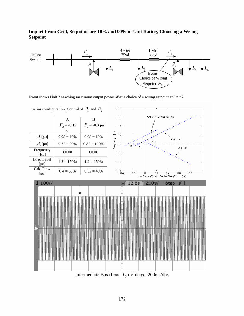
172

Import From Grid, Setpoints are 10% and 90% of Unit Rating, Choosing a Wrong Setpoint

Event shows Unit 2 reaching maximum output power after a choice of a wrong setpoint at Unit 2.

Intermediate Bus (Load 3L ) Voltage, 200ms/div.

Series Configuration, Control of 1P and 2F

A

2F = -0.12 pu

B

2F = -0.3 pu

1P [pu] 0.08 = 10% 0.08 = 10%

2P [pu] 0.72 = 90% 0.80 = 100% Frequency

[Hz] 60.00 60.00

Load Level [pu] 1.2 = 150% 1.2 = 150%

Grid Flow [pu] 0.4 = 50% 0.32 = 40%

Utility System

1P

1F

2P

2F

1L 3L 4L 5L

4 wire 75yd

4 wire 25yd

Event: Choice of Wrong

Setpoint 2F

173

Unit 1: P, Q, F, Frequency, Voltage Magnitude, Current Magnitude, 500ms/div.

Unit 2: P, Q, F, Frequency, Voltage Magnitude, Current Magnitude, 500ms/div.

174

Import From Grid, Setpoints are 10% and 90% of Unit Rating, Islanding Event shows Unit 2 reaching maximum output power after islanding.

Intermediate Bus (Load 3L ) Voltage, 200ms/div.

Series Configuration, Control of 1P and 2F

A – Grid B – Island

1P [pu] 0.08 = 10% 0.4 = 50%

2P [pu] 0.72 = 90% 0.8 = 100% Frequency

[Hz] 60.00 59.80

Load Level [pu] 1.2 = 150% 1.2 = 150%

Grid Flow [pu] 0.4 = 50% 0.0

Utility System

1P

1F

2P

2F

1L 3L 4L 5L

4 wire 75yd

4 wire 25yd

Event: Transfer to Island

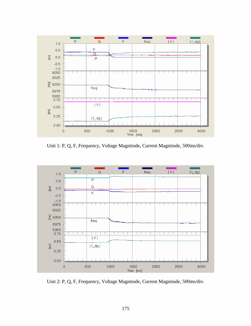
175

Unit 1: P, Q, F, Frequency, Voltage Magnitude, Current Magnitude, 500ms/div.

Unit 2: P, Q, F, Frequency, Voltage Magnitude, Current Magnitude, 500ms/div.

176

Island, Setpoints are 30% and 70% of Unit Rating, Load Removal Event shows Unit 2 backing off from maximum output power after a load is removed.

Intermediate Bus (Load 3L ) Voltage, 200ms/div.

Series Configuration, Control of 1P and 2F

A – 5L on B – 5L off

1P [pu] 0.4 = 50% 0.28 = 35%

2P [pu] 0.8 = 100% 0.62 = 77% Frequency

[Hz] 59.80 59.875

Load Level [pu] 1.2 = 150% 0.9 = 112%

Grid Flow [pu] 0.0 0.0

Utility System

1P

1F

2P

2F

1L 3L 4L 5L

4 wire 75yd

4 wire 25yd

Event: Load 5L Removal

177

Unit 1: P, Q, F, Frequency, Voltage Magnitude, Current Magnitude, 500ms/div.

Unit 2: P, Q, F, Frequency, Voltage Magnitude, Current Magnitude, 500ms/div.

178

Island, Setpoints are 10% and 90% of Unit Rating, Setpoint Change

Event shows Unit 2 backing off from maximum output power after setpoint of unit 2 has been changed.

Intermediate Bus (Load 3L ) Voltage, 200ms/div.

Series Configuration, Control of 1P and 2F

A

2F = -0.12 pu B

2F = 0.2 pu

1P [pu] 0.4 = 50% 0.44 = 55%

2P [pu] 0.8 = 100% 0.76 = 95% Frequency

[Hz] 59.80 59.775

Load Level [pu] 1.2 = 150% 1.2 = 150%

Grid Flow [pu] 0.0 0.0

Utility System

1P

1F

2P

2F

1L 3L 4L 5L

4 wire 75yd

4 wire 25yd

Event: Setpoint 2F Change

179

Unit 1: P, Q, F, Frequency, Voltage Magnitude, Current Magnitude, 500ms/div.

Unit 2: P, Q, F, Frequency, Voltage Magnitude, Current Magnitude, 500ms/div.

180

Import From Grid, Setpoints are 90% and 10% of Unit Rating, Choosing a Wrong Setpoint

Event shows Unit 2 reaching zero output power after a choice of a wrong setpoint at Unit 2.

Intermediate Bus (Load 3L ) Voltage, 200ms/div.

Series Configuration, Control of 1P and 2F

A

2F = 0.52 pu B

2F = 0.7 pu

1P [pu] 0.72 = 90% 0.72 = 90%

2P [pu] 0.08 = 10% 0.0 Frequency

[Hz] 60.00 60.00

Load Level [pu] 1.2 = 150% 1.2 = 150%

Grid Flow [pu] 0.4 = 50% 0.48 = 60%

Utility System

1P

1F

2P

2F

1L 3L 4L 5L

4 wire 75yd

4 wire 25yd

Event: Choice of Wrong

Setpoint 2F

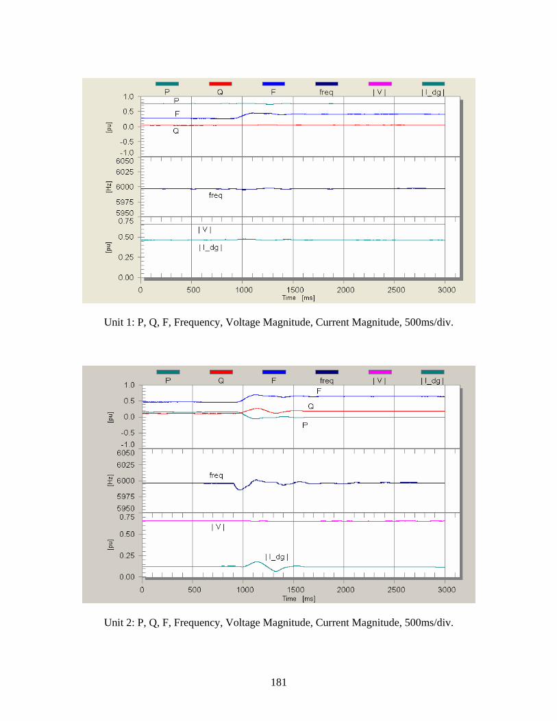
181

Unit 1: P, Q, F, Frequency, Voltage Magnitude, Current Magnitude, 500ms/div.

Unit 2: P, Q, F, Frequency, Voltage Magnitude, Current Magnitude, 500ms/div.

182

Import From Grid, Setpoints are 90% and 10% of Unit Rating, Islanding Event shows Unit 1 reaching maximum output power after islanding.

Intermediate Bus (Load 3L ) Voltage, 200ms/div.

Series Configuration, Control of 1P and 2F

A – Grid B – Island

1P [pu] 0.72 = 90% 0.8 = 100%

2P [pu] 0.08 = 10% 0.4 = 50% Frequency

[Hz] 60.00 59.80

Load Level [pu] 1.2 = 150% 1.2 = 150%

Grid Flow [pu] 0.4 = 50% 0.0

Utility System

1P

1F

2P

2F

1L 3L 4L 5L

4 wire 75yd

4 wire 25yd

Event: Transfer to Island

183

Unit 1: P, Q, F, Frequency, Voltage Magnitude, Current Magnitude, 500ms/div.

Unit 2: P, Q, F, Frequency, Voltage Magnitude, Current Magnitude, 500ms/div.

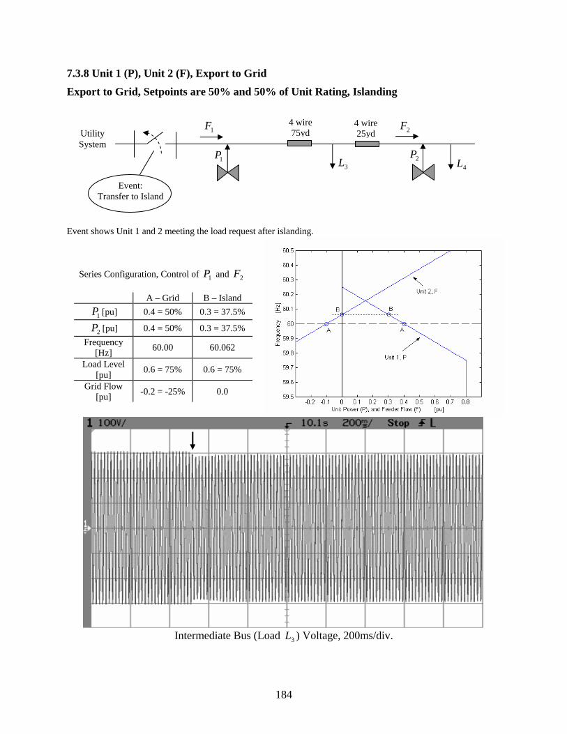
184

7.3.8 Unit 1 (P), Unit 2 (F), Export to Grid

Export to Grid, Setpoints are 50% and 50% of Unit Rating, Islanding Event shows Unit 1 and 2 meeting the load request after islanding.

Intermediate Bus (Load 3L ) Voltage, 200ms/div.

Series Configuration, Control of 1P and 2F A – Grid B – Island

1P [pu] 0.4 = 50% 0.3 = 37.5%

2P [pu] 0.4 = 50% 0.3 = 37.5% Frequency

[Hz] 60.00 60.062

Load Level [pu] 0.6 = 75% 0.6 = 75%

Grid Flow [pu] -0.2 = -25% 0.0

Utility System

1P

1F

2P

2F

3L 4L

4 wire 75yd

4 wire 25yd

Event: Transfer to Island

185

Unit 1: P, Q, F, Frequency, Voltage Magnitude, Current Magnitude, 500ms/div.

Unit 2: P, Q, F, Frequency, Voltage Magnitude, Current Magnitude, 500ms/div.

186

Export to Grid, Setpoints are 10% and 90% of Unit Rating, Islanding Event shows output power of Unit 1 going to zero after islanding.

Intermediate Bus (Load 3L ) Voltage, 200ms/div.

Series Configuration, Control of 1P and 2F

A – Grid B – Island

1P [pu] 0.08 = 10% 0.0

2P [pu] 0.72 = 90% 0.6 = 75% Frequency

[Hz] 60.00 60.075

Load Level [pu] 0.6 = 75% 0.6 = 75%

Grid Flow [pu] -0.2 = -25% 0.0

Utility System

1P

1F

2P

2F

3L 4L

4 wire 75yd

4 wire 25yd

Event: Transfer to Island

187

Unit 1: P, Q, F, Frequency, Voltage Magnitude, Current Magnitude, 500ms/div.

Unit 2: P, Q, F, Frequency, Voltage Magnitude, Current Magnitude, 500ms/div.

188

Export to Grid, Setpoints are 90% and 10% of Unit Rating, Islanding

Event shows Unit 2 reaching zero output power after islanding.

Intermediate Bus (Load 3L ) Voltage, 200ms/div.

Series Configuration, Control of 1P and 2F

A – Grid B – Island

1P [pu] 0.72 = 90% 0.6 = 75%

2P [pu] 0.08 = 10% 0.0 Frequency

[Hz] 60.00 60.075

Load Level [pu] 0.6 = 75% 0.6 = 75%

Grid Flow [pu] -0.2 = -25% 0.0

Utility System

1P

1F

2P

2F

3L 4L

4 wire 75yd

4 wire 25yd

Event: Transfer to Island

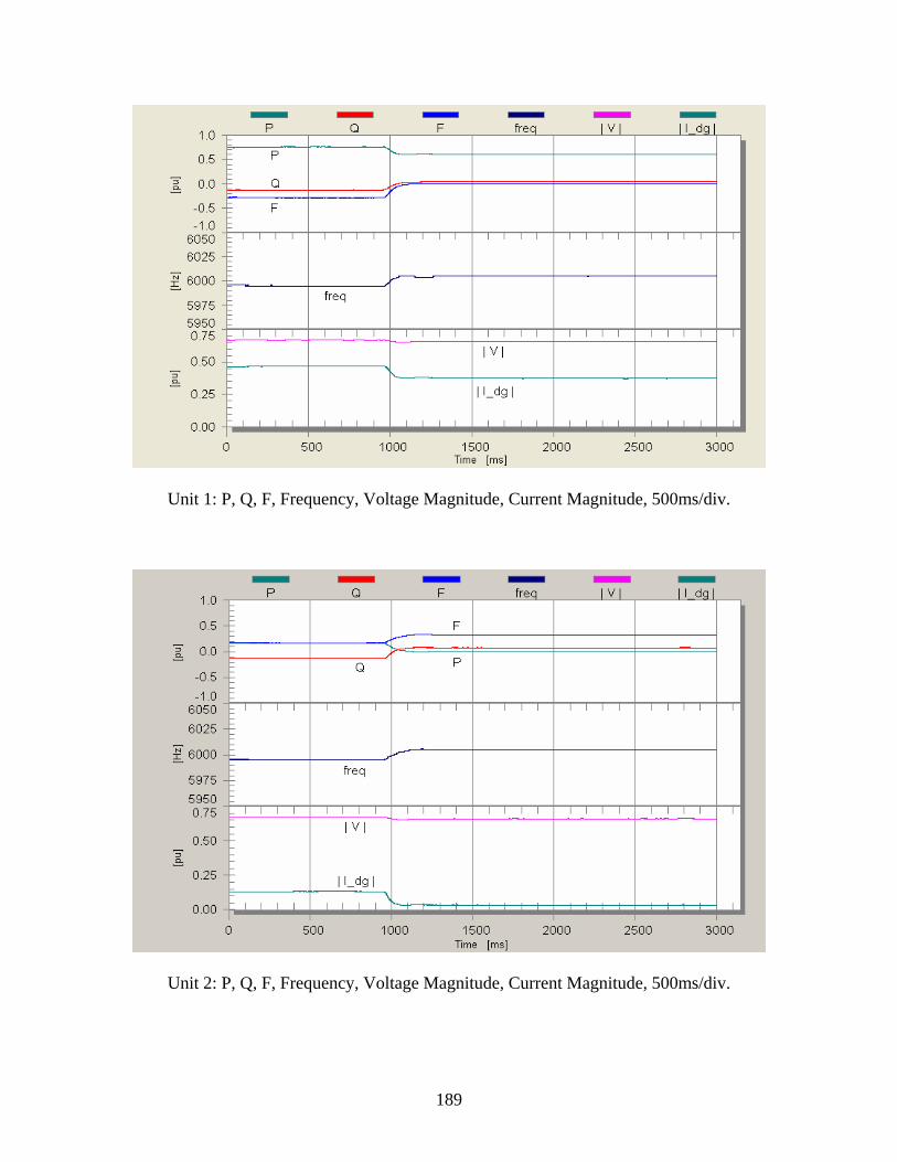
189

Unit 1: P, Q, F, Frequency, Voltage Magnitude, Current Magnitude, 500ms/div.

Unit 2: P, Q, F, Frequency, Voltage Magnitude, Current Magnitude, 500ms/div.

190

Island, Setpoints are 90% and 10% of Unit Rating, Load Insertion Event shows Unit 2 backing off from zero output power after a load is inserted.

Intermediate Bus (Load 3L ) Voltage, 200ms/div.

Series Configuration, Control of 1P and 2F

A – 5L off B – 5L on

1P [pu] 0.6 = 75% 0.62 = 77%

2P [pu] 0.0 0.28 = 35% Frequency

[Hz] 60.075 60.062

Load Level [pu] 0.6 = 75% 0.9 = 112%

Grid Flow [pu] 0.0 0.0

Utility System

1P

1F

2P

2F

3L 4L 5L

4 wire 75yd

4 wire 25yd

Event: Load 5L Insertion

191

Unit 1: P, Q, F, Frequency, Voltage Magnitude, Current Magnitude, 500ms/div.

Unit 2: P, Q, F, Frequency, Voltage Magnitude, Current Magnitude, 500ms/div.

192

Island, Setpoints are 90% and 10% of Unit Rating, Setpoint Change

Event shows Unit 2 backing off from zero output power after feeder flow setpoint of Unit 2 has been changed.

Intermediate Bus (Load 3L ) Voltage, 200ms/div.

Series Configuration, Control of 1P and 2F

A

2F = 0.22 pu B

2F = -0.1 pu

1P [pu] 0.6 = 75% 0.46 = 57%

2P [pu] 0.0 0.14 = 18% Frequency

[Hz] 60.075 60.162

Load Level [pu] 0.6 = 75% 0.6 = 75%

Grid Flow [pu] 0.0 0.0

Utility System

1P

1F

2P

2F

3L 4L

4 wire 75yd

4 wire 25yd

Event: Setpoint 2F Change

193

Unit 1: P, Q, F, Frequency, Voltage Magnitude, Current Magnitude, 500ms/div.

Unit 2: P, Q, F, Frequency, Voltage Magnitude, Current Magnitude, 500ms/div.

194

7.4 Parallel Configuration

This configuration represents the typical distribution system inside a building: there are feeders in parallel, each one with a source and loads scattered: some of them are near each of the two sources while another load is in an intermediate location between grid and unit 2. Figure 7.14 shows the general layout of the system with the series configuration.

Figure 7.14 Units in Parallel Configuration.

Utility System 1P

1F

2P

2F 1L

3L 4L 4 wire 75yd

4 wire 25yd

2L

5L

195

7.4.1 Unit 1 (F), Unit 2 (F), Import from Grid

Import From Grid, Setpoints are 50% and 50% of Unit Rating, Islanding Event shows Unit 1 and 2 meeting the load request after islanding.

Intermediate Bus (Load 3L ) Voltage, 200ms/div.

Parallel Configuration, Control of 1F and 2F

A – Grid B – Island

1P [pu] 0.4 = 50% 0.6 = 75%

2P [pu] 0.4 = 50% 0.6 = 75% Frequency

[Hz] 60.00 59.875

Load Level [pu] 1.2 = 150% 1.2 = 150%

Grid Flow [pu] 0.4 = 50% 0.0

Utility System 1P

1F

2P

2F 1L

3L 4L 4 wire 75yd

4 wire 25yd

Event: Transfer to Island

2L

196

Unit 1: P, Q, F, Frequency, Voltage Magnitude, Current Magnitude, 500ms/div.

Unit 2: P, Q, F, Frequency, Voltage Magnitude, Current Magnitude, 500ms/div.

197

Import From Grid, Setpoints are 10% and 90% of Unit Rating, Choosing a Wrong Setpoint Event shows Unit 2 reaching maximum output power after a choice of a wrong setpoint at Unit 2.

Intermediate Bus (Load 3L ) Voltage, 200ms/div.

Parallel Configuration, Control of 1F and 2F

A

2F = -0.42 pu B

2F = -0.6 pu

1P [pu] 0.08 = 10% 0.08 = 10%

2P [pu] 0.72 = 90% 0.8 = 100% Frequency

[Hz] 60.00 60.00

Load Level [pu] 1.2 = 150% 1.2 = 150%

Grid Flow [pu] 0.4 = 50% 0.32 = 40%

Utility System 1P

1F

2P

2F 1L

3L 4L 4 wire 75yd

4 wire 25yd

Event: Choice of Wrong

Setpoint 2F 2L

198

Unit 1: P, Q, F, Frequency, Voltage Magnitude, Current Magnitude, 500ms/div.

Unit 2: P, Q, F, Frequency, Voltage Magnitude, Current Magnitude, 500ms/div.

199

Import From Grid, Setpoints are 10% and 90% of Unit Rating, Islanding Event shows Unit 2 reaching maximum output power after islanding.

Intermediate Bus (Load 3L ) Voltage, 200ms/div.

Parallel Configuration, Control of 1F and 2F

A – Grid B – Island

1P [pu] 0.08 = 10% 0.4 = 50%

2P [pu] 0.72 = 90% 0.8 = 100% Frequency

[Hz] 60.00 59.80

Load Level [pu] 1.2 = 150% 1.2 = 150%

Grid Flow [pu] 0.4 = 50% 0.0

Utility System 1P

1F

2P

2F 1L

3L 4L 4 wire 75yd

4 wire 25yd

Event: Transfer to Island

2L

200

Unit 1: P, Q, F, Frequency, Voltage Magnitude, Current Magnitude, 500ms/div.

Unit 2: P, Q, F, Frequency, Voltage Magnitude, Current Magnitude, 500ms/div.

201

Island, Setpoints are 10% and 90% of Unit Rating, Load Removal Event shows Unit 2 backing off from maximum output power after a load is removed.

Intermediate Bus (Load 3L ) Voltage, 200ms/div.

Parallel Configuration, Control of 1F and 2F

A – 3L on B – 3L off

1P [pu] 0.4 = 50% 0.13 = 16%

2P [pu] 0.8 = 100% 0.77 = 96% Frequency

[Hz] 59.80 59.968

Load Level [pu] 1.2 = 150% 0.9 = 112%

Grid Flow [pu] 0.0 0.0

Utility System 1P

1F

2P

2F 1L

3L 4L 4 wire 75yd 4 wire

25ydEvent: Load 3L Removal

2L

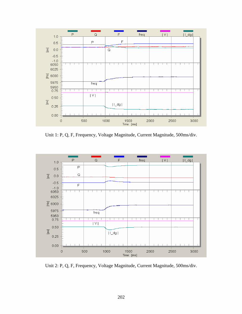
202

Unit 1: P, Q, F, Frequency, Voltage Magnitude, Current Magnitude, 500ms/div.

Unit 2: P, Q, F, Frequency, Voltage Magnitude, Current Magnitude, 500ms/div.

203

Island, Setpoints are 10% and 90% of Unit Rating, Setpoint Change Event shows Unit 2 backing off from maximum output power after setpoint of unit 2 has been changed.

Intermediate Bus (Load 3L ) Voltage, 200ms/div.

Parallel Configuration, Control of 1F and 2F

A

2F = -0.42 pu B

2F = -0.1 pu

1P [pu] 0.4 = 50% 0.44 = 55%

2P [pu] 0.8 = 100% 0.76 = 95% Frequency

[Hz] 59.80 59.775

Load Level [pu] 1.2 = 150% 1.2 = 150%

Grid Flow [pu] 0.0 0.0

Utility System 1P

1F

2P

2F 1L

3L 4L 4 wire 75yd

4 wire 25yd

Event: Setpoint 2F Change

2L

204

Unit 1: P, Q, F, Frequency, Voltage Magnitude, Current Magnitude, 500ms/div.

Unit 2: P, Q, F, Frequency, Voltage Magnitude, Current Magnitude, 500ms/div.

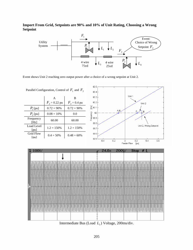
205

Import From Grid, Setpoints are 90% and 10% of Unit Rating, Choosing a Wrong Setpoint Event shows Unit 2 reaching zero output power after a choice of a wrong setpoint at Unit 2.

Intermediate Bus (Load 3L ) Voltage, 200ms/div.

Parallel Configuration, Control of 1F and 2F

A

2F = 0.22 pu B

2F = 0.4 pu

1P [pu] 0.72 = 90% 0.72 = 90%

2P [pu] 0.08 = 10% 0.0 Frequency

[Hz] 60.00 60.00

Load Level [pu] 1.2 = 150% 1.2 = 150%

Grid Flow [pu] 0.4 = 50% 0.48 = 60%

Utility System 1P

1F

2P

2F 1L

3L 4L 4 wire 75yd

4 wire 25yd

Event: Choice of Wrong

Setpoint 2F 2L

206

Unit 1: P, Q, F, Frequency, Voltage Magnitude, Current Magnitude, 500ms/div.

Unit 2: P, Q, F, Frequency, Voltage Magnitude, Current Magnitude, 500ms/div.

207

Import From Grid, Setpoints are 90% and 10% of Unit Rating, Islanding Event shows Unit 1 reaching maximum output power after islanding.

Intermediate Bus (Load 3L ) Voltage, 200ms/div.

Parallel Configuration, Control of 1F and 2F

A – Grid B – Island

1P [pu] 0.72 = 90% 0.8 = 100%

2P [pu] 0.08 = 10% 0.4 = 50% Frequency

[Hz] 60.00 59.80

Load Level [pu] 1.2 = 150% 1.2 = 150%

Grid Flow [pu] 0.4 = 50% 0.0

Utility System 1P

1F

2P

2F 1L

3L 4L 4 wire 75yd

4 wire 25yd

Event: Transfer to Island

2L

208

Unit 1: P, Q, F, Frequency, Voltage Magnitude, Current Magnitude, 500ms/div.

Unit 2: P, Q, F, Frequency, Voltage Magnitude, Current Magnitude, 500ms/div.

209

7.4.2 Unit 1 (F), Unit 2 (F), Export to Grid

Export to Grid, Setpoints are 50% and 50% of Unit Rating, Islanding Event shows Unit 1 and 2 meeting the load request after islanding.

Intermediate Bus (Load 3L ) Voltage, 200ms/div.

Parallel Configuration, Control of 1F and 2F A – Grid B – Island

1P [pu] 0.4 = 50% 0.3 = 37.5%

2P [pu] 0.4 = 50% 0.3 = 37.5% Frequency

[Hz] 60.00 60.062

Load Level [pu] 0.6 = 75% 0.6 = 75%

Grid Flow [pu] -0.2 = -25% 0.0

Utility System 1P

1F

2P

2F

3L 4L 4 wire 75yd

4 wire 25yd

Event: Transfer to Island

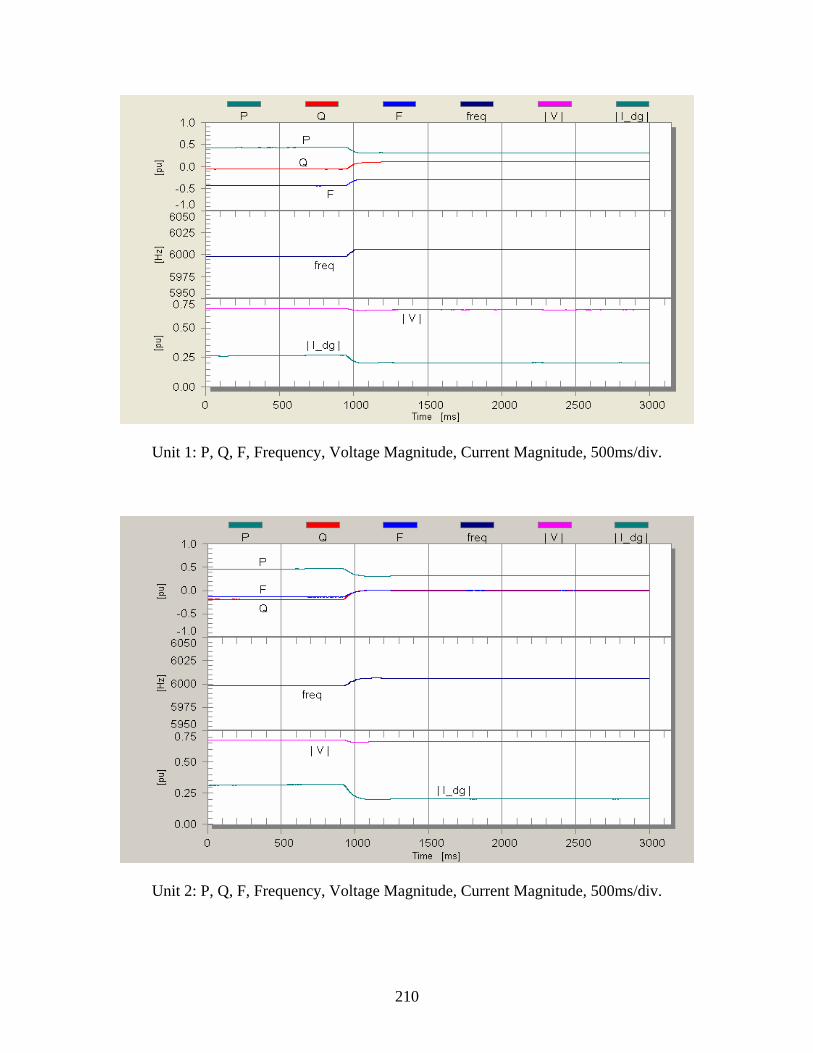
210

Unit 1: P, Q, F, Frequency, Voltage Magnitude, Current Magnitude, 500ms/div.

Unit 2: P, Q, F, Frequency, Voltage Magnitude, Current Magnitude, 500ms/div.

211

Export to Grid, Setpoints are 10% and 90% of Unit Rating, Islanding Event shows feeder flow and output power of Unit 1 going to zero after islanding.

Intermediate Bus (Load 3L ) Voltage, 200ms/div.

Parallel Configuration, Control of 1F and 2F

A – Grid B – Island

1P [pu] 0.08 = 10% 0.0

2P [pu] 0.72 = 90% 0.6 = 75% Frequency

[Hz] 60.00 60.075

Load Level [pu] 0.6 = 75% 0.6 = 75%

Grid Flow [pu] -0.2 = -25% 0.0

Utility System 1P

1F

2P

2F

3L 4L 4 wire 75yd

4 wire 25yd

Event: Transfer to Island

212

Unit 1: P, Q, F, Frequency, Voltage Magnitude, Current Magnitude, 500ms/div.

Unit 2: P, Q, F, Frequency, Voltage Magnitude, Current Magnitude, 500ms/div.

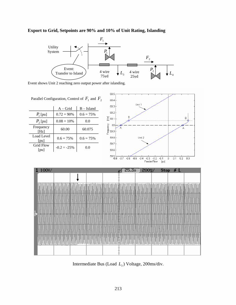
213

Export to Grid, Setpoints are 90% and 10% of Unit Rating, Islanding Event shows Unit 2 reaching zero output power after islanding.

Intermediate Bus (Load 3L ) Voltage, 200ms/div.

Parallel Configuration, Control of 1F and 2F

A – Grid B – Island

1P [pu] 0.72 = 90% 0.6 = 75%

2P [pu] 0.08 = 10% 0.0 Frequency

[Hz] 60.00 60.075

Load Level [pu] 0.6 = 75% 0.6 = 75%

Grid Flow [pu] -0.2 = -25% 0.0

Utility System 1P

1F

2P

2F

3L 4L 4 wire 75yd

4 wire 25yd

Event: Transfer to Island

214

Unit 1: P, Q, F, Frequency, Voltage Magnitude, Current Magnitude, 500ms/div.

Unit 2: P, Q, F, Frequency, Voltage Magnitude, Current Magnitude, 500ms/div.

215

Island, Setpoints are 90% and 10% of Unit Rating, Load Insertion Event shows Unit 2 backing off from zero output power and Unit 1 reaching maximum power output after a load is inserted.

Intermediate Bus (Load 3L ) Voltage, 200ms/div.

Parallel Configuration, Control of 1F and 2F

A – 1L off B – 1L on

1P [pu] 0.6 = 75% 0.8 = 100%

2P [pu] 0.0 0.1 = 12% Frequency

[Hz] 60.075 59.987

Load Level [pu] 0.6 = 75% 0.9 = 112%

Grid Flow [pu] 0.0 0.0

Utility System 1P

1F

2P

2F 1L

3L 4L 4 wire 75yd 4 wire

25yd

Event: Load 1L Insertion

216

Unit 1: P, Q, F, Frequency, Voltage Magnitude, Current Magnitude, 500ms/div.

Unit 2: P, Q, F, Frequency, Voltage Magnitude, Current Magnitude, 500ms/div.

217

Island, Setpoints are 90% and 10% of Unit Rating, Setpoint Change

Event shows Unit 2 backing off from zero output power after feeder flow setpoint of Unit 2 has been changed.

Intermediate Bus (Load 3L ) Voltage, 200ms/div.

Parallel Configuration, Control of 1F and 2F

A

2F = 0.22 pu B

2F = -0.1 pu

1P [pu] 0.6 = 75% 0.46 = 57%

2P [pu] 0.0 0.14 = 18% Frequency

[Hz] 60.075 60.162

Load Level [pu] 0.6 = 75% 0.6 = 75%

Grid Flow [pu] 0.0 0.0

Utility System 1P

1F

2P

2F

3L 4L 4 wire 75yd

4 wire 25yd

Event: Setpoint 2F Change

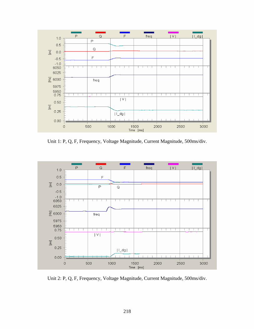
218

Unit 1: P, Q, F, Frequency, Voltage Magnitude, Current Magnitude, 500ms/div.

Unit 2: P, Q, F, Frequency, Voltage Magnitude, Current Magnitude, 500ms/div.

219

7.4.3 Unit 1 (F), Unit 2 (P), Import from Grid

Import From Grid, Setpoints are 50% and 50% of Unit Rating, Islanding Event shows Unit 1 and 2 meeting the load request after islanding.

Intermediate Bus (Load 3L ) Voltage, 200ms/div.

Parallel Configuration, Control of 1F and 2P

A – Grid B – Island

1P [pu] 0.4 = 50% 0.6 = 75%

2P [pu] 0.4 = 50% 0.6 = 75% Frequency

[Hz] 60.00 59.875

Load Level [pu] 1.2 = 150% 1.2 = 150%

Grid Flow [pu] 0.4 = 50% 0.0

Utility System 1P

1F

2P

2F 1L

3L 4L 4 wire 75yd

4 wire 25yd

Event: Transfer to Island

2L

220

Unit 1: P, Q, F, Frequency, Voltage Magnitude, Current Magnitude, 500ms/div.

Unit 2: P, Q, F, Frequency, Voltage Magnitude, Current Magnitude, 500ms/div.

221

Import From Grid, Setpoints are 10% and 90% of Unit Rating, Choosing a Wrong Setpoint Event shows Unit 1 reaching zero output power after a choice of a wrong setpoint at Unit 1.

Intermediate Bus (Load 3L ) Voltage, 200ms/div.

Parallel Configuration, Control of 1F and 2P

A

1F = 0.52 pu B

1F = 0.7 pu

1P [pu] 0.08 = 10% 0.0

2P [pu] 0.72 = 90% 0.72 = 90% Frequency

[Hz] 60.00 60.00

Load Level [pu] 1.2 = 150% 1.2 = 150%

Grid Flow [pu] 0.4 = 50% 0.48 = 60%

Utility System 1P

1F

2P

2F 1L

3L 4L 4 wire 75yd

4 wire 25yd

Event: Choice of Wrong

Setpoint 1F 2L

222

Unit 1: P, Q, F, Frequency, Voltage Magnitude, Current Magnitude, 500ms/div.

Unit 2: P, Q, F, Frequency, Voltage Magnitude, Current Magnitude, 500ms/div.

223

Import From Grid, Setpoints are 10% and 90% of Unit Rating, Islanding Event shows Unit 2 reaching maximum output power after islanding.

Intermediate Bus (Load 3L ) Voltage, 200ms/div.

Parallel Configuration, Control of 1F and 2P

A – Grid B – Island

1P [pu] 0.08 = 10% 0.4 = 50%

2P [pu] 0.72 = 90% 0.8 = 100% Frequency

[Hz] 60.00 59.80

Load Level [pu] 1.2 = 150% 1.2 = 150%

Grid Flow [pu] 0.4 = 50% 0.0

Utility System 1P

1F

2P

2F 1L

3L 4L 4 wire 75yd

4 wire 25yd

Event: Transfer to Island

2L

224

Unit 1: P, Q, F, Frequency, Voltage Magnitude, Current Magnitude, 500ms/div.

Unit 2: P, Q, F, Frequency, Voltage Magnitude, Current Magnitude, 500ms/div.

225

Island, Setpoints are 10% and 90% of Unit Rating, Load Removal Event shows Unit 2 backing off from maximum output power after a load is removed.

Intermediate Bus (Load 3L ) Voltage, 200ms/div.

Parallel Configuration, Control of 1F and 2P

A – 3L on B – 3L off

1P [pu] 0.4 = 50% 0.13 = 16%

2P [pu] 0.8 = 100% 0.77 = 96% Frequency

[Hz] 59.80 59.968

Load Level [pu] 1.2 = 150% 0.9 = 112%

Grid Flow [pu] 0.0 0.0

Utility System 1P

1F

2P

2F 1L

3L 4L 4 wire 75yd 4 wire

25ydEvent: Load 3L Removal

2L

226

Unit 1: P, Q, F, Frequency, Voltage Magnitude, Current Magnitude, 500ms/div.

Unit 2: P, Q, F, Frequency, Voltage Magnitude, Current Magnitude, 500ms/div.

227

Island, Setpoints are 10% and 90% of Unit Rating, Setpoint Change Event shows Unit 2 backing off from maximum output power after setpoint of Unit 2 has been changed.

Intermediate Bus (Load 3L ) Voltage, 200ms/div.

Parallel Configuration, Control of 1F and 2P

A

2P = 0.72 pu B

2P = 0.4 pu

1P [pu] 0.4 = 50% 0.44 = 55%

2P [pu] 0.8 = 100% 0.76 = 95% Frequency

[Hz] 59.80 59.775

Load Level [pu] 1.2 = 150% 1.2 = 150%

Grid Flow [pu] 0.0 0.0

Utility System 1P

1F

2P

2F 1L

3L 4L 4 wire 75yd

4 wire 25yd

Event: Setpoint 2P Change

2L

228

Unit 1: P, Q, F, Frequency, Voltage Magnitude, Current Magnitude, 500ms/div.

Unit 2: P, Q, F, Frequency, Voltage Magnitude, Current Magnitude, 500ms/div.

229

Import From Grid, Setpoints are 90% and 10% of Unit Rating, Choosing a Wrong Setpoint

Event shows Unit 1 reaching maximum output power after a choice of a wrong setpoint at Unit 1.

Intermediate Bus (Load 3L ) Voltage, 200ms/div.

Parallel Configuration, Control of 1F and 2P

A

1F = -0.12 pu B

1F = -0.3 pu

1P [pu] 0.72 = 90% 0.80 = 100%

2P [pu] 0.08 = 10% 0.08 = 10% Frequency

[Hz] 60.00 60.00

Load Level [pu] 1.2 = 150% 1.2 = 150%

Grid Flow [pu] 0.4 = 50% 0.32 = 40%

Utility System 1P

1F

2P

2F 1L

3L 4L 4 wire 75yd

4 wire 25yd

Event: Choice of Wrong

Setpoint 1F 2L

230

Unit 1: P, Q, F, Frequency, Voltage Magnitude, Current Magnitude, 500ms/div.

Unit 2: P, Q, F, Frequency, Voltage Magnitude, Current Magnitude, 500ms/div.

231

Import From Grid, Setpoints are 90% and 10% of Unit Rating, Islanding Event shows Unit 1 reaching maximum output power after islanding.

Intermediate Bus (Load 3L ) Voltage, 200ms/div.

Parallel Configuration, Control of 1F and 2P

A – Grid B – Island

1P [pu] 0.72 = 90% 0.8 = 100%

2P [pu] 0.08 = 10% 0.4 = 50% Frequency

[Hz] 60.00 59.80

Load Level [pu] 1.2 = 150% 1.2 = 150%

Grid Flow [pu] 0.4 = 50% 0.0

Utility System 1P

1F

2P

2F 1L

3L 4L 4 wire 75yd

4 wire 25yd

Event: Transfer to Island

2L

232

Unit 1: P, Q, F, Frequency, Voltage Magnitude, Current Magnitude, 500ms/div.

Unit 2: P, Q, F, Frequency, Voltage Magnitude, Current Magnitude, 500ms/div.

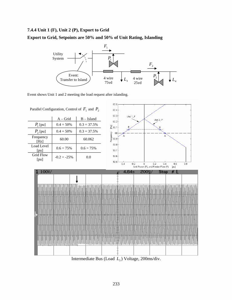
233

7.4.4 Unit 1 (F), Unit 2 (P), Export to Grid

Export to Grid, Setpoints are 50% and 50% of Unit Rating, Islanding Event shows Unit 1 and 2 meeting the load request after islanding.

Intermediate Bus (Load 3L ) Voltage, 200ms/div.

Parallel Configuration, Control of 1F and 2P A – Grid B – Island

1P [pu] 0.4 = 50% 0.3 = 37.5%

2P [pu] 0.4 = 50% 0.3 = 37.5% Frequency

[Hz] 60.00 60.062

Load Level [pu] 0.6 = 75% 0.6 = 75%

Grid Flow [pu] -0.2 = -25% 0.0

Utility System 1P

1F

2P

2F

3L 4L 4 wire 75yd

4 wire 25yd

Event: Transfer to Island

234

Unit 1: P, Q, F, Frequency, Voltage Magnitude, Current Magnitude, 500ms/div.

Unit 2: P, Q, F, Frequency, Voltage Magnitude, Current Magnitude, 500ms/div.

235

Export to Grid, Setpoints are 10% and 90% of Unit Rating, Islanding Event shows feeder flow and output power of Unit 1 going to zero after islanding.

Intermediate Bus (Load 3L ) Voltage, 200ms/div.

Parallel Configuration, Control of 1F and 2P

A – Grid B – Island

1P [pu] 0.08 = 10% 0.0

2P [pu] 0.72 = 90% 0.6 = 75% Frequency

[Hz] 60.00 60.075

Load Level [pu] 0.6 = 75% 0.6 = 75%

Grid Flow [pu] -0.2 = -25% 0.0

Utility System 1P

1F

2P

2F

3L 4L 4 wire 75yd

4 wire 25yd

Event: Transfer to Island

236

Unit 1: P, Q, F, Frequency, Voltage Magnitude, Current Magnitude, 500ms/div.

Unit 2: P, Q, F, Frequency, Voltage Magnitude, Current Magnitude, 500ms/div.

237

Export to Grid, Setpoints are 90% and 10% of Unit Rating, Islanding Event shows Unit 2 reaching zero output power after islanding.

Intermediate Bus (Load 3L ) Voltage, 200ms/div.

Parallel Configuration, Control of 1F and 2P

A – Grid B – Island

1P [pu] 0.72 = 90% 0.6 = 75%

2P [pu] 0.08 = 10% 0.0 Frequency

[Hz] 60.00 60.075

Load Level [pu] 0.6 = 75% 0.6 = 75%

Grid Flow [pu] -0.2 = -25% 0.0

Utility System 1P

1F

2P

2F

3L 4L 4 wire 75yd

4 wire 25yd

Event: Transfer to Island

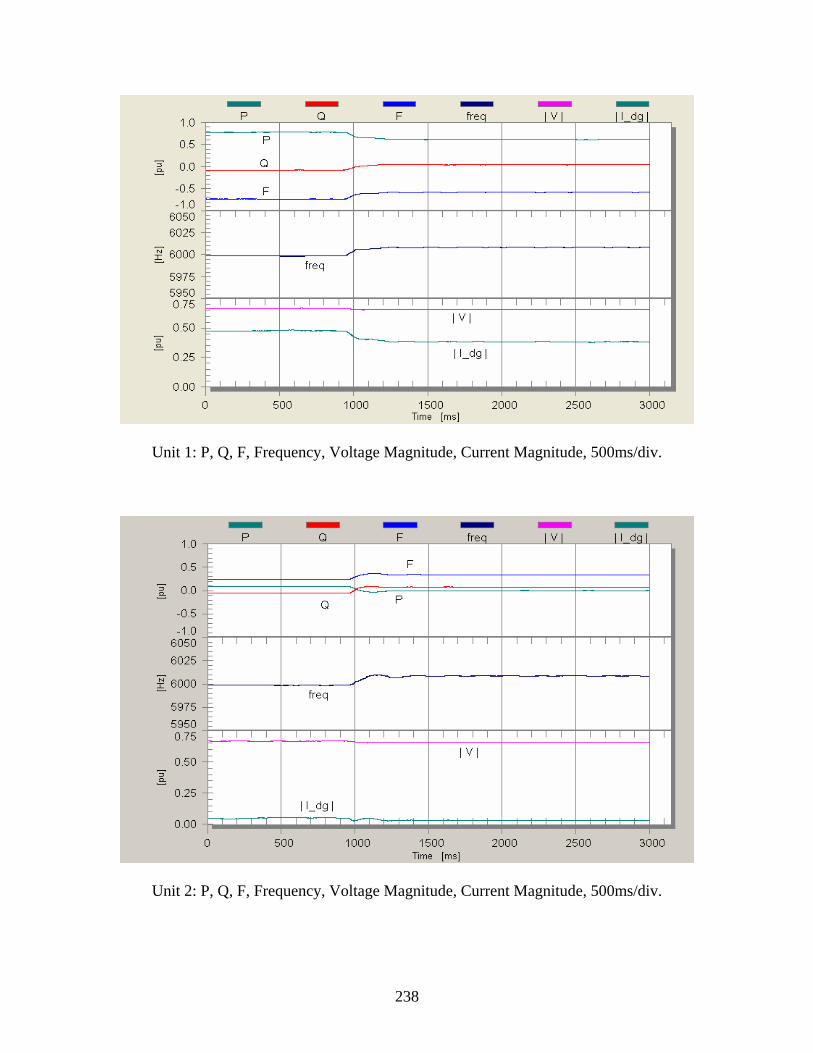
238

Unit 1: P, Q, F, Frequency, Voltage Magnitude, Current Magnitude, 500ms/div.

Unit 2: P, Q, F, Frequency, Voltage Magnitude, Current Magnitude, 500ms/div.

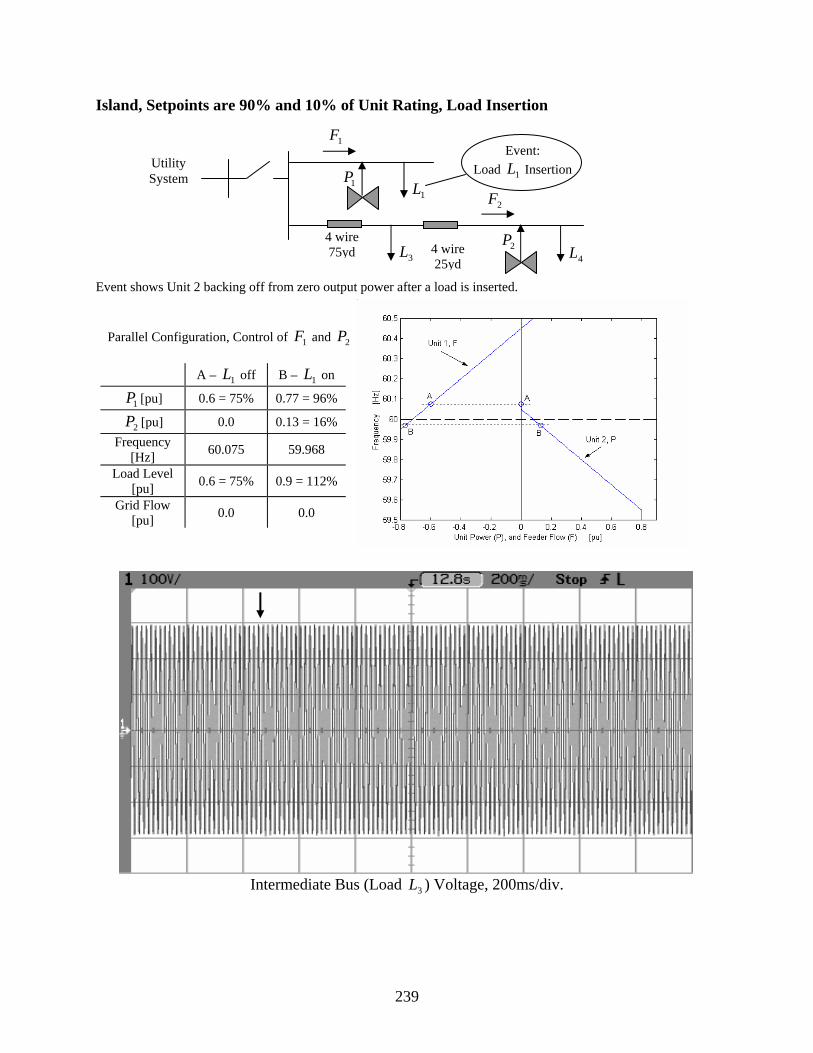
239

Island, Setpoints are 90% and 10% of Unit Rating, Load Insertion Event shows Unit 2 backing off from zero output power after a load is inserted.

Intermediate Bus (Load 3L ) Voltage, 200ms/div.

Parallel Configuration, Control of 1F and 2P

A – 1L off B – 1L on

1P [pu] 0.6 = 75% 0.77 = 96%

2P [pu] 0.0 0.13 = 16% Frequency

[Hz] 60.075 59.968

Load Level [pu] 0.6 = 75% 0.9 = 112%

Grid Flow [pu] 0.0 0.0

Utility System 1P

1F

2P

2F 1L

3L 4L 4 wire 75yd 4 wire

25yd

Event: Load 1L Insertion

240

Unit 1: P, Q, F, Frequency, Voltage Magnitude, Current Magnitude, 500ms/div.

Unit 2: P, Q, F, Frequency, Voltage Magnitude, Current Magnitude, 500ms/div.

241

Island, Setpoints are 90% and 10% of Unit Rating, Setpoint Change

Event shows Unit 2 backing off from zero output power after setpoint of Unit 2 has been changed.

Intermediate Bus (Load 3L ) Voltage, 200ms/div.

Parallel Configuration, Control of 1F and 2P

A

2P = 0.08 pu B

2P = 0.4 pu

1P [pu] 0.6 = 75% 0.46 = 57%

2P [pu] 0.0 0.14 = 18% Frequency

[Hz] 60.075 60.162

Load Level [pu] 0.6 = 75% 0.6 = 75%

Grid Flow [pu] 0.0 0.0

Utility System 1P

1F

2P

2F

3L 4L 4 wire 75yd

4 wire 25yd

Event: Setpoint 2P Change

242

Unit 1: P, Q, F, Frequency, Voltage Magnitude, Current Magnitude, 500ms/div.

Unit 2: P, Q, F, Frequency, Voltage Magnitude, Current Magnitude, 500ms/div.

243

Chapter 8. Conclusions

This work showed that the microgrid architecture is a viable solution for including distributed generation in a power system. This novel approach requires some features such as plug and play and peer to peer for each of the units in the subsystem to operate correctly.

These features created issues that needed to be solved in order to successfully implement them in a control for distributed generation. The control has been extensively tested on software simulations and then digitally implemented on hardware platform. The UW-Madison testbed includes two sources connected by four wire cables. Loads are located near each of the sources and on the long cable that separates them. The connection with the utility is realized with a static switch.

The UW-Madison microgrid setup allowed to test all the features of the control, including the units in series and parallel configuration by rearranging the wiring connectivity. The test exercised the upper and lower active power limits of the units when controlling source power injection and feeder power flow.

The results obtained in this testing phase are very encouraging because the units performed as expected without showing unknown behaviors. This first success has been the key motivator to push for a new series of larger scale testing at American Electric Power. Work is currently being carried out to create a three unit demo microgrid and subject it to a similar series of tests by the end of the year 2006.

Upon completing the tests at American Electric Power the next logical phase for RD&D is to build from the base established by the AEP Microgrid to prioritize, develop, and then demonstrate needed additional technology enhancements required to optimize the microgrid from the explicit perspective of enhancing the business case for microgrids. That is, having demonstrated the technical feasibility of microgrid functions, RD&D optimization efforts are now needed to accelerate commercial deployment. The work will pay special attention to the economic drivers outlined in the solicitation: “economic dispatch responsive to pricing signals and demand management programs, customer willingness to pay premiums for increased power reliability and quality, etc.”

244

REFERENCES [1] C.J.Melhorn, T.D. Davis, G.E.Beam, "Voltage Sags: Their Impact on the Utility and

Industrial Customers,", IEEE Transactions on Industry Applications, Vol.34, No.3, May/June 1998, pp.549-558.

[2] R.H. Lasseter, K. Tomsovic, P. Piagi, “Scenarios for Distributed Technology

Applications with Steady State and Dynamic Models of Loads and Micro-Sources,” Prepared for the Transmission Reliability Program Office of Power Technologies, Assistant Secretary for Energy Efficiency and Renewable Energy, U.S. Department of Energy http://certs.lbl.gov/pdf/PSERC_deri.pdf.

[3] P. Piagi, R. H. Lasseter, “Distributed Energy Resources Integration Industrial

Application of Microgrids,” Consortium for Electric Reliability Technology Solutions, Power System Engineering Research Center, University of Wisconsin-Madison, October 2001 http://certs.lbl.gov/pdf/Industry_Microgrid_6.pdf.

[4] R.H. Lasseter, P. Piagi, “Control of small distributed energy resources,” United States

Patent Application 20040051387. [5] B.Burger, A.Engler, “Fast Signal Conditioning in Single Phase Systems,” 9th European

Conference on Power Electronics and Applications, 27.-29.08.2001, Graz. [6] D.W. Novotny, T.A. Lipo, “Vector Control and Dynamics of AC Drives,” Clarendon

Press, Oxford, 1996. [7] M.F. McGranaghan, D.R. Mueller, M.J. Samotyj, “Voltage Sags in Industrial Systems,”

IEEE Transactions on Industry Applications, Vol. 29, No. 2, March/April 1993. [8] “American National Standard for Electrical Power Systems and Equipment,” Voltage

Ratings (60 Hertz), ANSI C84.1 -1995. [9] National Electrical Manufacturers Association (NEMA), Motors and Generators

MG 1-1987.

[10] T. Gonen, “Electric Power Distribution System Engineering,” McGraw-Hill, 1986. [11] Rome Cable Corporation, “Rome Cable Manual,” Rome Cable Corporation, Rome NY

1957. [12] Office of Energy Efficiency and Renewable Energy, U.S. Department of Energy, “2001

BTS Core Databook,” Office of Building Technology, July 13, 2001. [13] Marnay, C. and O. Bailey, “The CERTS Microgrid and the Future of the Macrogrid,”

LBNL-55281. August 2004.

245

[14] Lasseter, R.,” Microgrids,” IEEE PES Winter Meeting, January 2002. [15] Zang, H., M.Chandorkar, G. Venkataramanan, “Development of Static Switchgear for

Utility Interconnection in a Microgrid.” Power and Energy Systems PES, Feb. 24-26, 2003, Palm Springs, CA.