Contour pocketing computation using mathematical morphology

R. Molina-Carmona1, A. Jimeno2, M. Davia2,3

1Department of Computer Science and Artificial Intelligence 2 Department of Computer Science Technology and Computation

3 CAD/CAM Department of Spanish Footwear Research Institute (INESCOP)

University of Alicante Apdo. Correos 99

03080 Alicante, Spain.

Abstract Tool path generation problem is one of the most complexes in Computer Aided Manufacturing. Although some efficient algorithms have been developed to solve it, their technological dependency makes them efficient in only a limited number of cases. In the article we propose a model that will set apart the geometrical issues involved in the manufacturing process from the purely technology-dependent physical issues by means of a topological system. Presented in the paper there is a method for offsetting any kind of curve regardless of the machining technology (i.e. independent of any tool geometry: spherical, conical, toroidal and so on). Specifically, we use parametric cubic curves, which is one of the most general and popular models in CAD/CAM applications.

Keywords: Offset, Contour pocketing, mathematical morphology

1. Introduction

Pocket machining is a specific kind of machining process. It can be defined as the removing of material inside some boundary on a plane, following a zigzag path or a contour parallel path. In this paper we will focus on contour parallel paths or, simply, contour pocketing.

Traditionally, the problem of contour pocketing has been formulated on the basis of the calculation of the offset of a given curve [1, 2]. Offset curves are defined as the locus of the points which are at a constant distance d along the normal from the generator curve [3]. In a more formal way, let C(t)=(Cx(t),Cy(t)) be a curve defined in a space ℜ for parameter t, and a representation space ℜ2, designed on a plane (e.g. XY plane). Its offset Cd(t) with constant distance d is defined as [4, 5]:

)()()( tNdtCtCd ⋅+= (1) where N(t) is the unit normal vector of C(t), defined as follows:

22 )(')('))('),('(

)(tCtC

tCtCtN

yx

xy

+

−=

(2)

If C(t) is a parametric cubic curve its condition of regularity guarantees that the derivative C’(t)=(Cx’(t),Cy’(t))≠ (0,0), so N(t) is well defined to any curve C(t) that fulfils this condition. Specifically, Bézier and BSpline curves (which are the most common curves in CAD) easily fulfil this condition, so the offset curve can be obtained in this case, because every Bézier or BSpline curve is regular if there is no point whose derivative is 0. If the derivative is 0, the curve can be divided at this point following any known method [1].

This formulation is mathematically elegant but it has some drawbacks. On the one hand, the offset is only defined for constant distance, so these offsets are restricted to one radius tools (i.e. spherical, cylindrical and conical) and are not valid for more complex tools (toroidal, rectangular, “free-form” tools). On the other hand, the root in the denominator of equation 2 makes the offset of curve C(t) not polynomial or rational in general, even when C(t) is. So, an approximation must be used, instead of exact solutions.

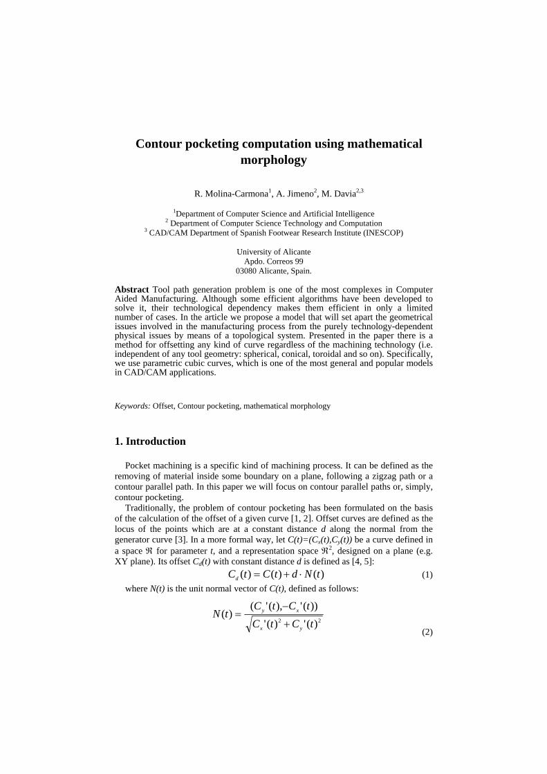
Some methods for approximating the offset have been proposed and they can be divided into two large groups: algorithms based on discretization, and analytic algorithms. The first group algorithms present problems with precision and, sometimes, with efficiency. The analytic algorithms are less versatile, because they cannot solve every case and they can be invalid.

Fig. 1. a) Raw offset of a curve. Local self-intersections in 1 and discontinuities in 2 will clash with part curve in shaded regions if it were machined. b) Offset after trimming self-intersections and avoiding the discontinuity. If this offset is used as a tool compensated trajectory, machined surface will differ from the original in 3 due to curve curvature.

Offset curves may self-intersect locally (when the offset distance is greater than the minimum radius of curvature in the concave regions) or globally (when the distance between two points on the curve reaches a local minimum). They can also have discontinuities in convex regions. So, an essential task for any approximation is to avoid the discontinuities and detect all self-intersections and trim the offset curve in a correct way (figure 1).

In [4] an interesting comparison of some of the offsetting methods can be found: control polygon-based methods, interpolation methods and circle approximation methods. Other authors prefer series approximation-based methods [5] or polygonal approximation methods [6].

Two major approaches have been used to solve the contour pocketing problem: direct offsetting approaches [6, 7] and Voronoi diagram approaches [8, 9, 10, 11]. In

3

b)

1 2

a)

the former set of procedures, the boundary curves are successively offset. They are very intuitive but again, self-intersection and discontinuity problems arise depending on surface curvature. Thus, more sophisticated and higher cost computing techniques are needed to detect and remove them, especially when islands appear.

The techniques based on the Voronoi diagram of the boundary use this diagram to trim the offset, so self-intersections are avoided. As a drawback, these kinds of methods are mainly suitable for a limited range of pocket shapes; they can have numerical errors and a high computational cost.

As a result of all the aforementioned methods, the main problems involved in contour pocketing techniques are: self-intersections, discontinuities, lack of generality (they are only suitable for one radius tools), inadequate precision, numerical errors and low efficiency.

Presented in the paper there is a new algorithm based on a new morphological approach [12] that avoids or solves the problems mentioned above. Due to the fact that the machining process is defined morphologically (an object, the tool, defines another object, the machined one), operators avoid the problem of self-intersections by its own definition. It is a versatile and general process, useful for every pocket shape and tool and highly efficient and precise. Once the offset calculation is done, the final tool path is obtained by a recursive procedure. Another important consideration is that we are only interested in the boundary of operations, since tool always attacks the material from inside in a contour pocketing process. Some efficient computation methods for morphology operations use the boundary representation as well [13, 14].

In section 2, a method to obtain the offset of a curve is presented. It is the basis of the algorithms described later, including that for contour-parallel machining. Section 3 shows some experiments and their results. Finally, conclusions are presented in section 4.

2. The morphological curve offset and pocketing

We present a method for offsetting any kind of curve. Specifically, we use parametric cubic curves, which are one of the most general models, and as such are very popular in CAD/CAM applications.

We are interested in defining the machining process itself, without technological considerations. A machining process could be described as the definition of an object (the shape) by means of another object (the tool). This idea is clearly related to a morphological operation, where the shape could be represented as a set X, and the tool could be modelled by a structuring element B. In this way, we could look at figure 1 and observe a morphologic dilation of the shape using a circle as a structuring element (SE). The compensated trajectory or offset corresponds to the dilation boundary.

A morphological operation will be divided into a sequence of unitary or basic operations. This sequence will guarantee the resulting order of the whole operation. Since every basic operation will correspond to a particular position of a tool along a

trajectory that is performed during a period of time, we call them instant basic operations.

This operation obtains the structuring element centre when it touches the X boundary following the vr direction. The concept is illustrated in figure 2. In that example, a shape X is transformed applying a 2D rotation matrix over its centre c. For this case, k could represent the number of degrees in that transformation matrix, so its values are in the [0,2π) range. Once the shape is transformed (figure 2.c), the distance between B and X in the vr direction is applied to the B centre in order to obtain the result of the instant basic operation (that is, the p point). For different and ordered real k values (using the < relation in ℜ), we will obtain a new set of structuring element centres that touch the X boundary. These centres will be also ordered in the geometric space due to the use of different rotation matrixes.

Fig. 2. Geometric description of the instant basic operator: a) Initial position. b) X transformation. c) Distance computing.

The instant basic operator can now be applied in order to achieve a whole morphologic operation. We are interested in defining one fundamental operation in the morphologic paradigm: the erosion. As commented above, the goal is obtaining only the boundary of these operations for offsetting purposes in contour pocketing processes.

Descriptively, this operation is classically defined as the place of centre positions of the structuring element B when it is forced to be inside an X set [15]:

{ }, ( )nyX B y R B In XΘ = ∈ ⊆

(3)

Where In(X) represents the inner part of a set, that is, X without periphery.

In our context, we are interested only in erosion boundary called Fr, which is the place of centre positions that touch the X frontier from inside:

{ }( ) : ( )ny yFr X B y R B In X B XΘ = ∈ ⊆ ∧ ∩ ≠ ∅ (4)

Derived from equation 3, we define the instant basic erosion, which defines a centre position touching the boundary of a set X, but from inside:

B X

vr c

a) c) B

vr p

c

X b) X B

vr c

( )n kΓ

( ) : ( )nk p pX B p R B X B In XΓΘ = ∈ ∩ ≠ ∅ ∧ ⊆ (5)

Using the instant basic erosion, we define the morphological offset of an X shape, as the set of points resulting from the repeated and ordered application of the instant basic erosion, for the normalized k range [0..1] (equation 6). Trajectory, defined by Γ(k), must assure the full round over the shape in the normalized range.

( ) { }( )[0..1]

: ( )nk y y

k

X B X B y R B X B In XΓ Γ∈

Θ = Θ = ∈ ∩ ≠ ∅∧ ⊆U (6)

Trajectory-based erosion, by means of homogeneous transformations which are compounded by translations and rotations, could orientate the structuring element in any position on the object boundary, this feature is not supported by classical dilations where the structuring element remains in the same position, but it is necessary when it is used for machining purposes (specially in 5-axis machining for tool orientation).

Fig. 3. Experiment in two dimensions. Shaded regions will not be machined. On the left, a morphological erosion for a toroidal tool (two radii implied). On the right, the classical offset for a spherical tool.

From the point of view of machining purposes, no specific structuring element geometry is given, that is, this method works for any structuring element geometry. In other words, the concept of offset (classically related to one radius tools) is here generalized, so even rectangular, elliptical or any geometry offset could be obtained. This is particularly useful to no standard pocketing, where other geometry tools are used (i.e. top piece moulds for heels in shoe making are made by means of torical tools with the rotating axe attacking parallel to the surface, in this special case two radii are implied in the machining process see left side of Fig. 4 and Fig. 6).

Original shape

morphologic operation frontiers

Fig. 4. Contour pocketing using a free form tool and a one radius tool. In a), a cylindrical tool producing a rectangular pocketing is shown. On the right, a comparative example: In b), the rectangle shape is machined correctly. In c), shaded regions are not machined because of the use of a one radius tool in classical pocketing.

For example, in figure 4c the shape cannot be correctly machined with a classical one-radius tool (some regions are not machined). However, a free form tool as proposed can correctly machine it and, so, would allow us to obtain a valid shape. Moreover, the use of several radii tools is very convenient to obtain optimal trajectories, that is, shorter tool paths that allow the system to machine the shape in a shorter time (see figure 3). This kind of material erosion could be obtained by means of tools as presented in figure 5 attacking in perpendicular direction on the machining plane.

Fig. 5 Different machining tools that could be used in tool paths as shown in figure 4.

max. depth distance

rotating axe

tool attack direction

rough material

Potential pocketing zone (tool shadow)

Cylindrical tool

a) b)

c)

Fig. 6. Contour pocketing examples using toroidal tools with the rotating axe parallel to surface.

The algorithm becomes simple if we apply the morphologic erosion concept defined in [15]. First of all, the curve C is discretized in a set of ordered points p along the length of the curve using a step s. For every point we compute the structuring element centre position (p’) that touches that point in a perpendicular direction (vp) from the shape inside. That centre p’ will be valid if the structuring element placed in p’ is inside the shape (that is, will not collide with the curve C). Obtaining a discrete model for computing the tool path implies a loss of precision. On the other hand, the algorithm becomes simpler and faster when a discrete model is used since there are no critical or singular situations. A discrete model of more or less definition can represent every curve. The proper step values will depend on the complexity of the curve.

A pseudo code algorithm is presented below: 1: For every pi ∈ C do 2: pi’= ObtainSECentre(pi,vpi); 3: If not CollideSE(pi’,C)then AddTrajectory(pi’) 4: Endfor

Algorithm 1. Basic pseudo-code algorithm for the morphological erosion

If a point p presents a discontinuity in first derivative, we generate a swept of new vectors in order to cover the gap (see figure 7). From that new set we also compute more possible structuring element centres.

Fig. 7. Analysis of s1 and s2 segments of shape C. Shaded SE positions are discarded due to shape collision. Note that discontinuity in pd is solved by a vector swept generation.

Algorithm cost analysis Computational cost is analysed in terms of the problem size for the algorithm

introduced in the algorithm 1. The operator used is O to determine an upper limit of the computation cost.

The basic algorithm consists in one external loop and two main function calls. The external loop, it is used to access to every point of the shape. Let n be the number of points that represent the shape C once it has been discretized. If we use a constant step factor s and the total length of C is L, then n will be L/s points.

The function ObtainSECentre computes the centre of the structuring element when it touches a point p in the direction addressed by the vp vector. So, this function depends of the SE geometry. For simple SEs as circles, rectangles, triangles, and so on, the function can be evaluated at constant time, we call this cost ct. Equation 7 shows this function for a circle tool with R in radius.

( , ) .p pObtainSECentre p v p R v= +uur uur

(7) Next function, called CollideSE(p’,C), returns true if the SE centred in the p’ point

is not completely inside the shape C and otherwise returns false. In order to evaluate this condition, this function computes the intersection of the SE geometry and the C shape. The cost of this function depends on the C representation. For the experiments we have discretized the shape into a set of contiguous segments that represents the shape within a defined maximum error. Then, every segment is tested (at a constant time), if a segment produces two or more intersections in the SE geometry then function returns true. Note that, in this case, discretization of C shape will be not the same that the previous one that we use to determine centre positions in shape. For shapes with a high degree of co linearity the number of segments will be reduced substantially. Let m be that number of segments. From experience we obtain m<<n.

Finally, the third function, called AddTrajectory, appends the new p’ centre to the list of successful centres at a constant time, so is not consider for evaluating cost purposes.

In order to obtain a good quality finish it is necessary to produce, at least, as many trajectory points as points the shape have. The finishing quality also depends on the

pi

p'i vp

pd

S1 S2

S3

S4

S5 pi+1

SE

material to be milled, for example, metallic ones produce best results but need more trajectory points than organic ones (plastics) and also more points (curve definition).

We analyse the whole algorithm in order to obtain an upper limit for the computational cost. Next expression evaluates the cost:

( )( ) ( ),limn m

n ct m O n m→∞

⋅ + = ⋅ (9)

As a guide, a usual value for s in shoe making is about 0.1mm obtaining a trajectory of two thousand points for a typical shape. On the other hand, m takes values of hundreds. In next sections we will show some quantitative examples.

Contour pocketing is carried out using a recursive algorithm that obtains successive interior general offsets to a given shape, (which can be a single or a multiple curve). Due to the morphological notation, even when there are islands, the algorithm works correctly. In figure 8 the operation of the algorithm and the recursion tree are shown.

An important aspect to control is which sections of the path must be followed at security height. This control is very complex in the recursive method. We alternatively propose an iterative method that uses a stack to simulate the recursions. The iterative version allows us to control the security height and to improve the efficiency of the method.

Fig. 8. Recursive algorithm for contour pocketing. The recursion tree can be easily simulated by a stack

The stack is used to store the calculated offsets, unstacking and adding them to the list of paths when the curve does not have offsets any further. This case is the same as the base case in the recursive algorithm, so unstacking simulates the procedure of going back in the recursion.

I1

O1

O

O11

O12 O13 O111

O112 O1121

O11211

O+I1

O1

O11 O12 O13

O111 O112

O1121

O11211

3. Experiments

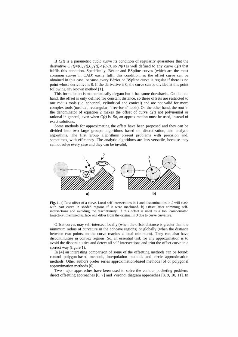
We present some experiments to prove four main properties of the morphological approach: generality, validity, optimality and efficiency.

Fig. 9. Offset of curves using the morphological approach. a) Offset with a one radius tool (e.g. spherical tool). b) Offset with a rectangular tool.

Generality is one of the main advantages of the morphological approach. This feature is referred to as the lack of any constraint in object or tool shape. By definition, no constraint is set up. In figures 9 and 10 some cases are shown.

Fig. 10. Contour pocketing using the morphological approach. a) Pocketing with a one radius tool (e.g. spherical tool). b) Pocketing with a rectangular tool.

b) a)

b) a)

Validity and optimality are consequences of generality. As there are no constraints in tool shape, it can be selected to correctly fit the object shape. As a result, it is easier to obtain a valid and optimal trajectory.

Validity is also achieved from the perspective of the correctness of the trajectory. One of the most powerful features of the morphological method is the fact that it is a formalization of the offset definition, instead of a geometrical or numerical method that approximates this definition. This is a very important feature, because geometrical or numerical problems are avoided. As a result, we can state that the morphological approach, from the theoretical point of view, allows us to obtain valid trajectories. From a practical perspective, it is easy to obtain an algorithm to implement the method, as we have shown in section 2.

Fig. 11. Contour pocketing using the morphological approach (left) and the commercial library (right). The library does not detect the two segments that are almost parallel.

The presented method has been compared with one of the most popular libraries, which is in fact the standard in commercial CAD/CAM systems. Although it is a very good library, it has some precision errors. Specifically, it fails when the angle between two consecutive segments is too close to 2π. The morphological method does not have this kind of problem, due to the fact that intersections, angles and other geometrical operations are not included in the definition of the formal method. Results are compared in figure 11.

Finally, some experiments have been done to prove the cost of the morphological method. In section 2.4 we defined n as the number of points that represent a given shape C once it has been discretized, and m the number of segments used to detect collisions. To prove that the cost of the morphological approach is O(n·m) (equation 9), we present a set of 50 experiments. Table 1 shows the results for 10 of the experiments, representing several kinds of shapes including all the geometrical cases (local and global self-intersections and discontinuities). It shows that, as we stated in section 2.4, m << n.

m n t (ms)

102 2370 31

158 5620 141

198 4772 156

200 3943 140

190 3071 109

161 2461 79

181 5772 172

296 10516 500

391 9702 609

444 6009 531

Table 1. Results for a sample of 10 experiments, n is the number of segments after discretization, m is the number of segments used to detect collisions and t is the time in milliseconds used to obtain the offset.

Figure 12 shows the results of the 50 experiments (including those in table 1), comparing n × m with the execution time in milliseconds. The time is very clearly related to n × m, so it proves that the theoretical cost O(n·m) is corroborated by the experiments.

Fig. 12. Results for a sample of 50 experiments. Time of execution (t) compared with the product of n and m: t is linearly dependent of n × m.

4. Discussion and conclusions

A method to obtain offsets based on the possibility of using different tool shapes has been presented. Current offset methods seldom consider this possibility, because of the multiple cases and peculiarities that make the process very costly and not robust.

The use of non-standard tools can be very interesting to machine complex topology pieces, so that the remaining material is minimized. Moreover, different tools could

0

500

1000

1500

2000

2500

3000

0 2000000 4000000 6000000 8000000 10000000 12000000 14000000

m x n

t

be chosen depending on the piece shape to improve the machining process. Specifically, the main advantages of using adapted tools are:

− Machining time can be substantially reduced. − The machine and the tool can be used in a proper way. − The machined piece would have a higher quality. − The time used to plan tool paths and to test them can be reduced. A general offset can allow us to use non-classical tools to obtain better results.

Some special tools can be found to be adapted to some specific tasks. They differ from standard spherical or toroidal tool path generation, so standard machining libraries do not usually deal with them. Some examples will be shown. Squared-end and corner radius tools

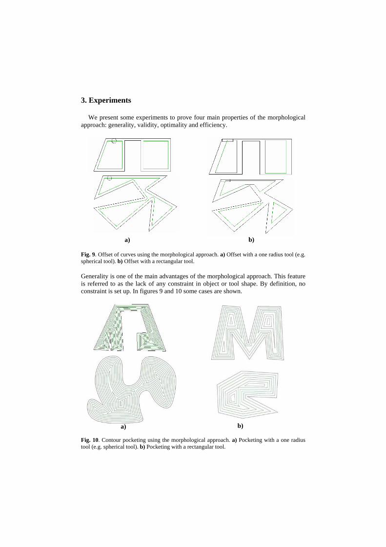
This kind of tools are usually chosen for rough milling and lateral wall finishing, as well as box bottom, especially when corners need to be machined with small radius tools.

They can also be use to toroidal machining. In this process the tool path is successively selfcrossed. The tool advances following a pattern of constant radius arcs. Square end tools with sharp corners can only be used in toroidal machining when there is no bottom in the piece. Nevertheless, corner radius can be used to toroidal machining with several cut depths (figure 13).

Fig. 13. Squared-end tool and machining example. Toroidal tools with polygonal section

Toroidal tools are used to mill boxes, cavities and male pieces with medium range speed and high quantities of wastes. A better use of toroidal tools is finishing plane surfaces, including partition lines (figure 14).

Fig. 14. Toroidal tools with polygonal section

Conical tools They are used in pencil tracing machining and areas with difficult access, specially

if there are right angles between adjacent walls (figure 15).

Fig. 15. Conical Tool

As a conclusion, a morphological model has been presented. We develop, through

trajectory-based morphological operations, a topological system resulting from the application of the conventional morphological model to which the feature of primitive ordering has been added. The proposed operations account for the problems present in the manufacturing processes derived from the tool machining. The implementation of the new morphological primitives, now machining operations, performed in the actual manufacturing process for validation. As a result, a new formalism to define and obtain generalized offsets is presented. This new formulation, based on morphology, avoids the main problems of the traditional methods, such as self intersections, discontinuities and lack of generality. Specifically, the main features of our method are:

− The use of morphology as the base of the formulation avoids certain problems by its own definition: self intersections and discontinuities do not exist in our approach, so they do not have to be treated in any way.

− The object to be machined and the tool are free-form shapes, so the method is general and versatile, useful for every pocket shape and tool without any constraint.

− As free form tools can be used, we can obtain optimal paths to get correct objects by just choosing the best fitting tool.

− The method is based on very simple and accurate calculations, so most numerical and geometrical problems are avoided.

− Obtaining the practical algorithm from the theoretical formulation is straightforward, as it has been shown in section 2. The resulting procedure is simple and efficient.

We are now working on adapting the formulation approach to three dimensional machining. The method could be especially useful in 5-axis machining. However, the

computing cost of the algorithm could be a bottle neck for three dimensions due to the high discretization effect. An extra effort must be made to improve and optimize the algorithm efficiency in 3D.

There are other morphological operations such as dilations, openings, closures etc. which could be useful in the machining domain. We are interested in demonstrating their utility and efficiency for surface reconstruction or trajectory optimization.

5. References

[1] Farin G (1993) Curves and Surfaces for Computer Aided Geometric Design. A Practical Guide. Academic Press, Inc, San Diego, USA.

[2] Wang, Y. Intersection of offsets of parametric surfaces. Computer Aided Geometric Design, vol. 13, pp.453-465, 1996.

[3] Maekawa T (1999) An overview of offset curves and surfaces. Computer-Aided Design 31:165-173.

[4] Elber G, Lee I.K, Kim M.S (1997) Comparing Offset Curve Approximation Methods. IEEE Computer Graphics & Applications 17,3:62-71.

[5] Li Y.M, Hsu V.Y (1998) Curve offsetting based on Legendre series. Computer-Aided Geometric Design 15:711-720.

[6] EL-Midany T.T, Elkeran A, Tawfik H (2002) A Sweep-Line Algorithm and Its Application to Spiral Pocketing. International Journal of CAD/CAM 2,1:23-38

[7] Park S.C, Choi B.K (2001) Uncut free pocketing tool-paths generation using pair-wise offset algorithm. Computer-Aided Design 33:739-746.

[8] O’Rourke J (1993) Computational Geometry in C. Cambridge University Press, Cambridge, UK.

[9] Lambregts C.A.H, Delbressine F.L.M, de Vries W.A.H, van der Wolf A.C.H (1996) An efficient automatic tool path generator for 2 ½ D free-form pockets. Computers in Industry 29,3:151-157.

[10] Held M (1998) Voronoi Diagrams and Offset Curves of Curvilinear Polygons. Computer-Aided Design 30,4:287-300.

[11] Jeong J, Kim K (1999) Generating Tool Paths for Free-Form Pocket Machining Using z-Buffer-Based Voronoi Diagrams. Int. J. Adv. Manuf. Technol 15:182-187.

[12] Jimeno, A.; Maciá, F.; García-Chamizo, J. (2004) Trajectory-based morphological operators: a morphological model for tool path computation, Proceedings of the international conference on algorithmic mathematics & computer science, AMCS 2004, Las Vegas (USA). Jun 2004.

[13] Vincent, L. (1991) Morphological transformations of binary images with arbitrary structuring elements. Image Processing, vol. 22, no. 1, pp. 3-23

[14] Nikopoulos, N., Pitas, I. (1997) An Efficient Algorithm for 3D Binary Morphological Transformations with 3D Structuring Elements of Arbitrary Size and Shape. Proceedings of 1997 IEEE Workshop on Nonlinear Signal and Image Processing (NSIP'97).

[15] Serra, J. (1982) Image Analysis and Mathematical Morphology. Academic Press, London.