continuous- time security pricing - darrell duffie · continuous- time security pricing a utility...

Journal of Mathematical Economics 23 (1994) 107-131. North-Holland

Continuous- time security pricing A utility gradient approach*

Darrell Duffie

Stanford University, Stanford CA, USA

Costis Skiadas

Northwestern Unioersity, Evanston IL, USA

Submitted January 1993, accepted May 1993

We consider a (not necessarily complete) continuous-time security market with semimartingale prices and general information filtration. In such a setting, we show that the first-order conditions for optimality of an agent maximizing a ‘smooth’ (but not necessarily additive) utility can be formulated as the martingale property of prices, after normalization by a ‘state-price’ process. The latter is given explicitly in terms of the agent’s utility gradient, which is in turn computed in closed form for a wide class of dynamic utilities, including stochastic differential utility, habit-forming utilities, and extensions.

Key words: Continuous time; Asset pricing; State prices; Martingale method; Stochastic differential utility; Habit formation; Dynamic utility

JEL classification: G12

1. Introduction

This paper presents a version of the idea of Harrison and Kreps (1979), linking the first-order conditions of portfolio optimality to the martingale property of normalized security prices, that leads to explicit asset pricing formulas with not necessarily additive utilities.

We consider a continuous-time security market where prices are modeled by semimartingales (allowing for jumps, and therefore incorporating discrete time as a special case). The underlying information filtration is general, and the market is not necessarily complete. In such a setting, we show that the first-order conditions for optimality of an agent maximizing a ‘smooth’ utility can be formulated as the martingale property of prices, after normalization

Correspondence to: Costis Skiadas, J.L. Kellogg Graduate School of Management, North- western University, 2001 Sheridan Road, Evanston, IL 60208-2006, USA.

*Duftie acknowledges the support of the National Science Foundation under NSF 2ACC488. We are grateful for the comments of Monique Jeanblanc-Picqut.

030~4068/94/%07.00 0 1994 Elsevier Science B.V. All rights reserved SSDJ 03044068(93)EOO53-X

108 D. Du@e and C. Skiadas, Continuous-time security pricing

by a ‘state-price’ process. The latter is given explicitly in terms of the agent’s utility gradient, which is in turn computed in closed form for a wide class of dynamic utilities, including the stochastic differential utility of Duflie and Epstein (1992); habit-forming utilities of the type used by Ryder and Heal (1973), Constantinides (1990), and Sundaresan (1989); as well as those discussed by Hindy and Huang (1992) over cumulative consumption processes, and generalizations of the above. This analysis is of interest mainly for the equilibrium asset pricing formulas under non-additive utilities. It also provides an essential intermediate step in the solution of the associated equilibrium and optimal portfolio problems.

The Harrison-Kreps (1979) argument consists of two parts: in the first part a separating-hyperplane argument is used to derive a strictly positive extension of the pricing functional, and in the second this extension is used to derive the martingale property of prices under appropriate normalization. In this paper we make no topological assumptions. The first-order conditions replace the separating-hyperplane argument, and they are used directly to derive the martingale property of normalized prices. (Of course the latter also defines a strictly positive extension of the pricing functional,) The ‘non-empty interior’ assumption required to apply the separating-hyperplane argument of Harrison and Kreps is replaced by an assumption that certain perturbations of the optimal trading strategy are feasible. This condition of feasible directions can be stated in a number of ways, and can be somewhat delicate in the case where consumption can occur only at rates. The argument is considerably simpler when consumption can occur in ‘lumps’.

Following Foldes (1990) and Back (1991), we consider a security market where prices are general semimartingales. As Bichteler and Dellacherie have shown, semimartingales are, in some sense, the most general type of processes that can be used as integrands of stochastic integrals. In this sense, they are the most general type of price processes with respect to which we can meaningfully define gains from trading. The reader unfamiliar with semimartingale theory will have little difficulty following the arguments of this paper, by accepting certain properties of semimartingales and Ito’s lemma at a formal level. All the required theory (as well as the Bichteler- Dellacherie theorem) can be found in Protter (1990).

The ‘martingale method’ for solving optimal portfolios has been developed in papers such as Pliska (1986), Cox and Huang (1989), Karatzas et al. (1991) and He and Pearson (1991). All these papers assume a time-separable expected utility, and as a result the analysis of the first-order conditions, and the computation of the state-price process can be carried out separately for each pair of state-of-the-world and time. This simplification is not possible with the more general type of utilities considered here. Related work is also reported by Kandori (1988) in discrete-time, and by Foldes (1990) and Back (1991) in continuous time. All of the above references assume time-separable

D. Dujfie and C. Skiadas, Continuous-time security pricing 109

expected utilities. Detemple and Zapatero (1991) apply the results of this paper to solve the optimal portfolio problem for a habit-forming utility under Brownian information and complete markets. (Their paper does not deal with the arguments that lead to the formula for state prices in terms of the utility gradient.) More comments on the optimal portfolio problem are given in the concluding remarks.

The rest of this paper is organized as follows: The primitives of the market model and the basic definitions are presented in section 2. Section 3 discusses the first-order conditions for optimality. Section 4 makes the connection between the first-order conditions for optimality and the martingale property of normalized prices. The case of absolutely continuous cumulative consumption requires some additional technical arguments presented in section 5. Section 6 introduces a general class of utilities with temporal dependencies, with various examples. The gradients of these utilities are computed in section 7. Finally, section 8 contains concluding remarks, and the appendices contain proofs and auxiliary mathematical results.

2. Preliminaries

We consider a finite time horizon [0,7’j and a filtered probability space (12, %, [F, P). [The infinite-horizon case is briefly discussed in section 8, and more extensively in Skiadas (1992).] The filtration IF = {%Gr : t 2 O> is assumed to satisfy the usual conditions,’ and, for simplicity, %,, is taken to be trivial, in that it contains only events of probability one or zero. We also assume that %-,=%. The expectation operator with respect to P is denoted E, and the corresponding conditonal expectation given 8, is denoted E,. All equality statements between random variables are in the almost sure sense with respect to P.

We take as primitive a convex set X of semimartingales. Any element C of X represents some cumulative consumption process, meaning that for every time t, C, represents the total net consumption up to, and including, time t. The initial value Co of a consumption process C represents an initial lump of consumption (that can also be interpreted as free disposal of initial wealth). We assume throughout that Co 20 for every CE X. (Typically, cumulative consumption processes are also assumed to be non-decreasing, but we are not going to need that property in any of our arguments.)

An agent, fixed throughout the paper, is characterized by a utility function U : X + R, and a semimartingale W representing a cumulative private endow- ment. There are N + 1 securities available for trading. The nth security (n=O, 1 , . . . , N) is characterized by a cumulative dividend process D" and

‘That is, F is right-continuous, and .F,, contains all null events. 2Protter (1990) and Dellacherie and Meyer (1982) are general references on semimartingale

theory and stochastic integration.

110 D. Duffie and C. Skiadas, Continuous-time security pricing

an ex-dividend price process S”, both of which are semimartingales. Let D - [DO,. . . ,DN] and S=[S’,... ,SN]. Security prices and dividends are all measured in common consumption units. A trading strategy is any vector- valued process of the form 8~ [e” ,. . . , ON], with each component a real- valued, locally bounded, predictable process.

The gain process G is defined as G = S+ D. The agent’s net ex-dividend gains, when following trading strategy 8, are given by the stochastic integral3 J0dG. A trading strategy 8 finances consumption C in X, using securities (S,D), if the following budget equations hold:4

eT qs, + AD,) = dcT

e;(S,+dD,)= j 8,dG,-C,_, t~C0,T-j. o-

The statement ‘0 finances C using (S,D)’ is compactly denoted 0UC. A price deflator is any strictly positive semimartingale. Given deflator j?,

and any semimartingale Y that represents a cumulative quantity (in our setting these are the elements of X, the components of D, and W), we define YB by letting: Y~E/?~Y~ and dYt=p,_ dK+ d[/I, Y-J,, t~[0, T]. On the other hand, if Y is a process that represents a non-cumulative quantity (such as S”, nE{O,..., IV}), we define YB =/3,E;, t E [O, 7’J We also let SB = [SOS,. . . , SNs], Da E [DOB , . . . , D”@], and GB E SB + DO. A special case of the following lemma is given in Huang (1985):

Lemma 1. For all CEX and any deflator /I,

t3UC if and only if 0u CB.

We take as primitive a set IZ of price deflators. For technical convenience, we assume that GB is integrable’ for all /?EIZ. In formulating the agent’s optimization problem, we wish to exclude pathological trading strategies, such as doubling strategies, that generate expected gains from trade even when the security gain process is a martingale. This sort of pathology should be impossible under any reasonable class of state price processes. Further- more, we only allow trading strategies that finance feasible consumption

‘For the purposes of this analysis, we treat j19dG as the sum ~~zO~OndG”. It is known, however, that this definition of an integral with respect to a multivariate semimartingale is rather limited, especially in its connection with martingale representation results. For the more general definition, also suitable for our purposes, see Jacod and Shiryaev (1987).

4Given any process Y with left limits, Y- denotes the process {q- : t E[O, T]}, with the convention that YO- ~0, and AYE Y- Y-. We also follow the notational convention that c _ q, dx = q.d Y. + ji Q d x, whenever the quantities involved are meaningful.

5That is, E 1 G:” 1 < co for all t and n.

D. Dufjie and C. Skiadas, Continuous-time security pricing 111

plans. We summarize these requirements in the following detinition. A trading strategy 8 is admissible if

(a) For any ~EH and n~{0,..., N} such that GnB is a martingale, ~8”dG”~ is also a martingale.

(b) There exists C E X such that 0-C - W.

We denote the set of admissible strategies 0.

Example 1. Suppose J7= {a: GB~xZ} # @, with 2’ defined in Appendix B. Using the facts of Appendix B, we can show that every LCRL (Left Continuous and with Right Limits) 0 such that E[(sup, 18, I)‘] < 00 satisfies condition (a) of the above definition. The requirement that n = @ is not very severe. In fact, given any price deflator fi, there is always a measure equivalent to P and with bounded Radon-Nikodym derivative under which GBe%’ [see Dellacherie and Meyer (1982, VII.58 and 63)].

A pair (0, C), consisting of an admissible trading strategy and a consumption plan, is budget feasible if 8uC and &, . GO + CO 5 W,. A budget feasible pair (8, C) is optimal if, for any other budget feasible (0, C), we have V(C) s U(C).

3. First-order conditions for optimality

In this section we state our basic assumption on the nature of the utility U, and we state the first-order conditions for optimality as a ‘no-expected- gains’ condition.

Throughout the paper, we fix a reference budget-feasible pair (8, C). A pair (0, C), where 0 is a trading strategy and C is a semimartingale, is a feasible direction if 0-C and (8, C) +s(& C) is in 0 x X for all sufficiently small positive E. We denote by F, and F, the projections of the feasible direction set F on X and 0, respectively. The following basic assumption on the nature of the utility U is maintained from this point.

Assumption 1. The Gateaux derivative6 vU(c, C) exists for all C in F,. Futhermore, there exists 7c in n such that, for all C in F,, V U(c C) = E(C;).

The process 71 is the Riesz representation of VU at C. Intuitively, the above assumption requires the existence of a strictly positive marginal utility

6The Gateaux derivative V U(c; .) : F+ R is defined by

VU(C;C)Glim u(C+aC)-U(C), &F, 010 a

provided the limit exists and is finite. If linear, VU(c;) is the gradient of U at c. Luenberger (1969) is a general reference on Gateaux derivatives and their use in optimization theory.

112 D. Dufie and C. Skiadas, Continuous-time security pricing

density II,(W) for consumption at time t and state of the world w. For example, if U(C) = E[jc u(dCJdt) dt] for smooth u: R+R and absolutely continuous C, then mild regularity implies that n, =u’(dC,/dt). In section 5, we show that Assumption 1 is satisfied for smooth versions of most dynamic utilities used in practice (under mild technical conditions), including a wide variety of (not necessarily separable utilities for which the Riesz representation rr is given explicitly in closed form. The assumption that rt is a semimartingale is of technical importance, and is further discussed in the concluding remarks.

It is convenient for us to extend the definition of U to 0 by letting U(0) = U(C), whenever 0-C. Clearly, the restriction of U to 0 also has a Gateaux derivative at 8, given by

VU(B;@=E(C”), (~,C)EF.

Also, we observe that (8, C) is optimal if and only if B is optimal, in the sense that

BEarg max{U(8):8E@, &,~G,~W,}.

The Lagrangian for this problem is given by: _Y ((&A) = U(e) + A( W, - 8,. G,), and the associated Slater condition is stated in the following assumption:

Assumption 2. BO. Go < W, for some 8 E 0.

Assumption 2 is a mild condition. For example, it is satisfied if W, > 0 and 0 E 0. The Saddle-Point Theorem states [see, for example, Holmes (1975, Theorem 14G)] that if 0 is optimal and the Slater condition is satisfied, then there exists 120 such that

9 (8, n) 2 2 (63 L 9 (e,3, ed, 220. w-v

Conversely, if the saddle-point condition, (SPC), is satisifed for some 220, then B is optimal.

Lemma 2. Under Assumption I, (SK) implies

ZJ; in addition, U is concave, then (FOC) implies (SIT).

ProoJ: The first-order necessary conditions for (SPC), that are also sufticient under concavity of U, are:

D. Duffie and C. Skiadas, Continuous-time security pricing 113

But if (0, C) EF, Assumption 1 and Lemma 1 imply that VU@ Q=E(C”,)= E(& 0,dG:). Cl

4. Martingale characterization of optimality

In this section we provide conditions under which optimality of (8, c) is equivalent to the martingale property of G”. The importance of the latter in the theory of asset pricing is well known. In particular, G” is a martingale if and only if

S,=;E, ( i(n,_dD,+ d[n,D],)+X& >

, tEC0, rl.

If the components of D are of finite the standard asset pricing formula:

variation, the above equation reduces to

Also, the martingale property characterizes short-term interest rates. To show that, let us assume that security zero represents short-term borrowing, in the sense that So z 1 and Do is of bounded variation. If K is a special semimartingale (for example, if it has bounded jumps) then it has a unique decomposition 7c= M + A, where M is a local martingale, A is of bounded variation and predictable, and A, =O. If Gon= X+~A dD” is a martingale, then it must be that the bounded variation part is constant. Therefore dDf = -dA,/n,. For the case in which A is absolutely continuous, we have dA, = pt dt, for some adapted process p, and dDF = I, dt, where I, = -p,/n,, a familiar formula for the short-term interest rate process [see, for example, Cox et al. (1985)].

The martingale property immediately implies optimality under concavity of the utility function:

Proposition I. Suppose Assumption 1 holds, U is concave, and G” is a martingale.’ Then (8, c) is optimal.

Proof: If G” is a martingale, then (FOC) holds with I= no, and the result follows by Lemma 2. 0

‘That is, G”” is a martingale, for every n.

114 D. Dufle and C. Skiadas, Continuous-time security pricing

In the remainder of this section, we concern ourselves with the converse of this result, for which additional assumptions are required (although concavity is not needed). Our argument will make use of the following well- known lemma [see, for example, Dellacherie and Meyer (1982, VI.13.)]:

Lemma 3. An integrable adapted process {I’, : t E [0, Tj} is a martingale if and only if EY, = E Y, for every stopping time r.

Consider the trading strategy, denoted 8(n,z), that holds one unit of security n from time 0 up to a stopping time z, and nothing else. In symbols,

0(n, 7): - 1 (OSt5r, i=n).

Lemma 4. Suppose that Assumptions I and 2 hold, and that f&n, Z)E F, for every stopping time z. Then optimality of B implies that G”” is a martingale.

Proof: By Lemma 2, (FOC) holds for some X20. In particular, with 8= + e(n, z), for any stopping time r, we obtain that E(Gp) =JG”,. In particular, when r =O, we conclude that either G”,=O, or X= no (or both). In either case, Lemma 3 applies, giving the martingale property of G”“. 0

Of course if the assumptions of Lemma 4 are satisfied for each n, we can conclude that G” is a martingale. More generally, we can adopt the following assumption:

Assumption 3. Given any stopping time z, and any security n#O, there exists a trading strategy 0, such that:

(a) fe~F,.

(b) 0: = l{ojtjr). (c) ek=O, for all k${O,n}.

In addition, + e(O, z) E Fe.

For example, parts (b) and (c) of Assumption 3 are satisfied by P= e(n, z). More generally, Assumption 3 allows for the possibility that the dividends of security n up to time z, and the gains (or losses) after it is sold at time r, are not necessarily consumed, but can be partly or fully invested in security zero.

Proposition 2. Suppose that Assumptions 1, 2, and 3 hold. Then optimality of 8 implies that G” is a martingale.

Proof: By Lemma 4, Go” is a martingale. We will now show that, given any n # 0, G”” is also a martingale. Let r be any stopping time, and 8” a trading

D. Dufie and C. Skiadas, Continuous-time security pricing 115

strategy satisfying the conditions of Assumption 3. Condition (FOC) and the fact that +~“EF, and Go” is a martingale, imply that

The proof is then completed just as in Lemma 4. IJ

One limitation of the above approach is that cumulative consumption must be allowed to jump. In many utility and equilibrium models, however, cumulative consumption is assumed to be absolutely continuous, and the above arguments do not apply. In the following section we deal with that technical issue. Since the basic ideas are the same as those of this section (modulo some approximation procedures) the reader can go directly to section 6 on a first reading.

5. The case of absolutely continuous consumption

In this section we show that a version of Proposition 2 can be formulated even when cumulative consumption is restricted to be absolutely continuous.

We begin with a generalization of Proposition 2, and then show how it applies to the case of absolutely continuous consumption. The following generalizes Assumption 3:

Assumption 4. Given any stopping time z and security n, there exists a sequence {e(m):m= 1,2,.. . } of trading strategies, such that

(a) &0(m) E F,, for every m. (b) On {t 5 z}, 0”(m) = 1 and f?(m) =O, for all k 4 (0, n} and all m.

(4 lim,,, E(JT e,(m) dG:) = 0.

The intuition behind Assumption 4 is as follows. For n =O, it postulates the existence of a sequence of trading strategies that, up to time r, hold a unit of security zero and none of the others, while all dividends are consumed. After time r consumption is increased so that all available wealth is consumed very fast, as expressed by condition (c). For n#O, Assumption 4 postulates the existence of a sequence of strategies that, up to time r, hold one unit of security n, and none of the others except for security zero, which is used to store all wealth created by unconsumed dividends. After time 7, all wealth is quickly consumed in the sense of condition (c). Finally, in all of the above cases, the corresponding consumption plans and their negatives must be feasible perturbations of C.

The following generalizes Proposition 2:

116 D. Dugie and C. Skiadas, Continuous-time security pricing

Proposition 3. Under Assumptions 1, 2 and 4, optimality of I!J implies that G” is a martingale.

Proof: The proof consists of mimicking the arguments of Lemma 4 and Proposition 2, with the trading strategies e(m) of Assumption 4 in place of ~(O,Z) and 8”. We then obtain, for any n and stopping time r, that

The result then follows by letting m+oz, and applying Lemma 2.

In the following example we introduce a setting of absolutely continuous cumulative consumption, and we give conditions under which Proposition 3 applies.

Example 2. We define a linear space 59 of processes, by letting CE~ if and only if

C,=C,+jc,dt, t<T, 0

for some progressively measurable integrable process c. In this example, we assume that X s%‘. Notice that a cumulative consumption C in X may still have a jump on the terminal date T, which is another way of saying that the terminal value of the portfolio may affect the agent’s utility. The only other restriction placed on X is that it is an order interval. More precisely, let 5 represent the order induced on V by the usual positive cone of non- decreasing processes. Then we assume that for all x,y EX, and any z E%?, xsz Iy implies that z EX. We let E be the progressively measurable process such that dC, = ~,dt, t < T. In this example we assume that security zero represents short-term borrowing; in particular, for all t E [0, T-J SF = 1 and Dp = so r, ds for some progressively measurable integrable process r.

Given any security n and any C E %7, let

d( 0: - C,) + AC,, tEC0, Tl.

This is the cum-dividend value process [0(S + AD)] associated with a trading strategy (0) that holds a unit of security n, finances cumulative consumption C, and reinvests all remaining dividends in short-term borrowing or lending

D. Duffe and C. Skiadas, Continuous-time security pricing 117

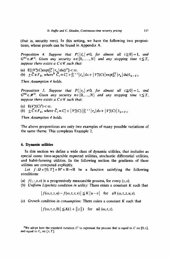
(that is, security zero). In this setting, we have the following two propositions, whose proofs can be found in Appendix A.

Proposition 4. Suppose that P{ 1 E, 1 ~0, for almost all t lo} = 1, and G’“E&‘~. Gioen any security nE (0,. . . . . N} and any stopping time 24 T, suppose there exists a CEW such that:

(a) H(W?ex~j~ 1 r,,j W21 < *. (b) fc’~F~, where’ C,=C;+S:“‘)&Ids+ IV:(C)(exp(jT(r,Idu)ll,=r,.

Then Assumption 4 holds.

Proposition 5. Suppose that P{ ) r, I ~0, for almost all t lo} = 1, and G’“E~‘. Given any security nE (0,. . ., N} and any stopping time 75 T, suppose there exists a CEW such that:

(a) (b)

E( y(C)‘) < 00. +CEF~, where e,=C:+ 1 V:(C)I~:“Ir,(ds+ ) V:(C)1 lft=Tj.

Then Assumption 4 holds.

The above propositions are only two examples of many possible variations of the same theme. This completes Example 2.

6. Dynamic utilities

In this section we define a wide class of dynamic utilities, that includes as special cases: time-separable expected utilities, stochastic differential utilities, and habit-forming utilities. In the following section the gradients of these utilities are computed explicitly.

Let f : Sz x [0, T] x R” x R-+08 be a function satisfying the following conditions:

(a) f(*;, z, u) is a progressively measurable process, for every (z, v). (b) Un$orm Lipschitz condition in utility: There exists a constant K such that

If(w,t,z,u)-f(O,t,z,0)I 5Klu-ol for all(o,t,z,u,u).

(c) Growth condition in consumption: There exists a constant K such that

(f(w,4z,O)( SK(l+ ~~z~~) for all (a,4z).

sWe adopt here the standard notation C to represent the process that is equal to C on [O,r], and equal to C, on [r, T].

118 D. Du@e and C. Skiadas, Continuous-time security pricing

We take as primitive a function 2 on X, valued in9 %“r [L2(Q x [O, T], 0, A)ln (the power n denoting a Cartesian product), where 0 is the optional o-algebra,” and 1 is the product measure of P and Lebesgue measure on [O,ZJ (restricted to 0). The space 3 is equipped with the usual norm:

(1~11 =(E)Izt[/idt)1'2, zcd.

The class of utilities we will be considering is characterized by the following result of Duffie and Epstein (1992):”

Theorem 1. For every C E X, there exists a unique process V(C) such that

4 .L(ZAC), K(C)) ds > 3 tECQT3. *

Throughout this section, and the next one, we assume that the utility U : X+Iw is given by U(C) = V,(C), where V(C) is the unique process of Theorem 1.

Remark. The discussion of this section and the next one can be extended in a straightforward way by adding a term g(dCr) in the integrand of the utility expression in the statement of Theorem 1, where g is assumed to satisfy a growth condition. This extension allows for the possibility that utility depends on the final payoff. For simplicity, we only consider the case of g=o.

Example 3 (stochastic differential utility). In the setting of Example 2, suppose Z,(C) = c, whenever dC, = c, dt, t < IT: and assume that Z(C) E 3’ for any CEX. Then U assumes a form of stochastic differential utility studied by DulIie and Epstein (1992). For example, when f takes the form ft(c,v)= u,(c) - ptv, we recover the classical time-separable utility over consumption- rate processes:

U(c)=E 0

‘For simplicity, we assume that 2 is valued in an L2 space. All the arguments to follow extend immediately to the case where Z is valued in some LP space, p 2 1.

“‘The optional a-algebra is generated by the RCLL (Right-Continuous and with Left Limits) adapted processes.

“Dufftie and Epstein (1992) in fact prove the result in a slightly more general setting in which Z is valued in an Lp space for some p > 1. Antonelli (1992) extends the argument to the case of p=l.


Example 4 (habit formation). In the setting of Example 2, habit formation can be modeled by defining the function 2, so that Z,(C) =(ct, z,), where dC, = c, dt, t < T, and

zt = z. + j h(c,, z,)ds, teC0, q, 0

for some h : R2+R that is uniformly Lipschitz in its second argument and satisfies a growth condition in its first argument. Again we assume that Z(C) E ?,Y for any C EX. This is a generalization, suggested by Duftie and Epstein (1992), of the habit-forming utilities adopted by Ryder and Heal (1973), Sundaresan (1989), and Constantinides (1990). There is of course no difficulty in extending this example (and its continuation in the next section) to the case in which h is state and time dependent.

Example 5 (Hindy-Huang-Kreps utilities). Another formulation of habit formation is suggested by Hindy and Huang (1992), extending the work of Hindy, Huang and Kreps (1992) in a space of cumulative consumption processes. Their model can be incorporated in our setting, by simply defining: Z,(C)=Sbk,_,dC,, where k is a progressively measurable bounded process.

7. Computation of utility gradients

In this section we explicitly compute the Gateaux derivative of the dynamic utilities just introduced, and give an explicit formula for the Riesz representation of the utility gradient in each of the examples of the last section.

The following smoothness assumption will be used:

Assumption 5. The process Z has a square-integrable uniform Gateaux derivative at C, meaning that, for every C in F,, there is a process AZ(c; C) in 3 such that:

lim sup AZ,(C;C)_ z’(c’ac)-z’(c) =O.

al0 f II a I/

Assumption 6. f,(w, ., .) is continuously differentiable for all (0, t), and there exists a constant K such that

Il$$w)~l SK(l+ Ilzll), (0,Z,V)EQXR”XR, tc[O,T-J.

120 D. DuJie and C. Skiadas, Continuous-time security pricing

Theorem 2. Under Assumptions 5 and 6, the Gateaux derivative VU(c C) exists for all C in Fx, and is given by:

where

iI3 af,(z,(e),~(~)VZ,(C;C)dt O taz

The above result can be used directly in computing the Riesz representation of utility gradients:

Example 3 (continued). In the case of stochastic differential utility, we have VZ,(c; C)=c,, whenever dC, =c,dt, t < T. Under Assumption 6, it follows from Theorem 2 that U has a utility gradient at C with Riesz representation:

rr,=B&,v,), tE[O,7--J.

Example 4 (continued). The uniform gradient of Z for the case of habit formation is given in the following result:

Lemma 5. Suppose that h is continuously dzrerentiable, ah/&z satisfies a growth condition in consumption,” and ah/& is bounded. Then Assumption 5 is satisfied, and

v&(C;C)=($$, bexp(j~(Z.(C))du)~(Z.(C))dC,).

Suppose now that Assumption 6, and the assumptions of Lemma 5 are satisfied. Then an application of Theorem 2 and Fubini’s theorem13 shows that U has a utility gradient at C with Riesz representation:

where the obvious arguments have been omitted.

“That is, there exists constant K such that 1 c%(c,z)/dc 1 5 K( 1 + 1 c I), for all (c, z). ‘jThe version of Fubini’s theorem for conditional expectations that we need here can be

found, for example, in Ethier and Kurtz (1986, Proposition 4.6).


Example 5 (continued). In Example 5, since 2 is linear, we have VZ(C; C) = Z,(C). Again by Fubini’s theorem, it follows from Theorem 2 that under Assumption 6, U has a utility gradient at C with Riesz representation:

8. Concluding remarks

We conclude this paper with a discussion of some related issues and unanswered questions.

lnjinite horizon. The extension of the contents of this paper to an inlinite- horizon setting is straightforward, after requiring that for every admissible trading strategy 8, and any rr in ZZ, lim f_ ,&Jt. S: = 0. The utility gradient computations also extend without much difficulty. The details are all spelled out in Skiadas (1992).

Equilibrium existence. There is as yet no equilibrium result of any kind for the space of cumulative consumption processes considered by Hindy and Huang (1992), except for the result by Mas-Cole11 and Richard (1991) in the case of certainty. Neither is there any result in continuous time for equilibrium without dynamically complete markets. A complete markets equilibrium existence result in a continuous-time setting in which agents maximize stochastic differential utility [of Duflie and Epstein (1992)] is presented by Duflie, Geoffard and Skiadas (1992).

Representative agents and semimartingale state prices. Huang (1987) shows how Constantinides’ (1982) demonstration of a representative agent in linite- dimensional settings can be extended to an appropriate continuous-time setting with additive utility. Aside from its own merits, the existence of a representative agent is important in order to establish that there exists a semimartingale equilibrium state price process, that is, a price deflator rcell such that G” is a martingale. For example, with a single agent maximizing a time-separable utility over consumption-rate processes, and having additive utility index u, if the aggregate consumption (rate) level w is a semimartingale, and if u is C3, then rr= u’(w) is the Riesz representation of the utility gradient and, by Ito’s lemma, is a semimartingale. With heterogeneous agents, the assumption of complete markets and smooth additive utilities satisfying Inada conditions implies the same result, since the representative agent’s utility function is additive and (by the implicit function theorem) smooth. [See Huang (1987).] From this, we can recover the consumption- based capital asset pricing model of Breeden (1979) directly from the tirst-


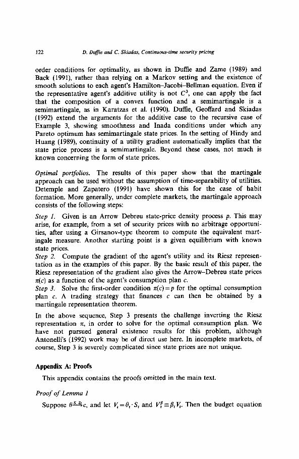
order conditions for optimality, as shown in Duffie and Zame (1989) and Back (1991), rather than relying on a Markov setting and the existence of smooth solutions to each agent’s Hamilton-Jacobi-Bellman equation. Even if the representative agent’s additive utility is not C3, one can apply the fact that the composition of a convex function and a semimartingale is a semimartingale, as in Karatzas et al. (1990). Duffie, Geoffard and Skiadas (1992) extend the arguments for the additive case to the recursive case of Example 3, showing smoothness and Inada conditions under which any Pareto optimum has semimartingale state prices. In the setting of Hindy and Huang (1989), continuity of a utility gradient automatically implies that the state price process is a semimartingale. Beyond these cases, not much is known concerning the form of state prices.

Optimal portfolios. The results of this paper show that the martingale approach can be used without the assumption of time-separability of utilities. Detemple and Zapatero (1991) have shown this for the case of habit formation. More generally, under complete markets, the martingale approach consists of the following steps:

Step 1. Given is an Arrow-Debreu state-price density process p. This may arise, for example, from a set of security prices with no arbitrage opportunities, after using a Girsanov-type theorem to compute the equivalent martingale measure. Another starting point is a given equilibrium with known state prices. Step 2. Compute the gradient of the agent’s utility and its Riesz representation as in the examples of this paper. By the basic result of this paper, the Riesz representation of the gradient also gives the Arrow-Debreu state prices X(C) as a function of the agent’s consumption plan c. Step 3. Solve the first-order condition z(c)=p for the optimal consumption plan c. A trading strategy that finances c can then be obtained by a martingale representation theorem.

In the above sequence, Step 3 presents the challenge inverting the Riesz representation rr, in order to solve for the optimal consumption plan. We have not pursued general existence results for this problem, although Antonelli’s (1992) work may be of direct use here. In incomplete markets, of course, Step 3 is severely complicated since state prices are not unique.

Appendix A: Proofs

This appendix contains the proofs omitted in the main text.

Proof of Lemma 1

Suppose 0uc, and let K = 8; S, and F’f -b, l$ Then the budget equation


gives dy = 8,(dG, - AD,) - dC, + AC,. In particular, A r/; = 8,A S,, which implies that l$ = q -A K = 19, * S, _ . The rest of the proof is an exercise in integration by parts for semimartingales [see Dellacherie and Meyer (1982, VIII.18) or Protter (1990, 11.6)]. We have

=/I-(B,(dG,-AD,)-dC,+AC,)

= et@-ds, +S,-dB,+dCB, Xl, + B,(dD, - AD,) +d[& D- AD],)

-B,(dC,-AC,)-dCB,C-Acl

= UWV,) + A - dD, + W 01,

-l&W -A-G -4X Cl, +B,AG

= 8,(dG; - AD!) - dC; + AC!.

The converse is the same result applied to B- ‘. To see this we note that if Y is any of SD, G, C, or I/, then (Y ) fi i/p= I: We now prove this in the non-obvious case, in which Y represents a cumulative quantity:

d(YB):,P=~(B~_dr;+d[A rl,)+d f ;, JB-dY+CB, Yl 1 f J;dg+@d;+ $,/I ,Y t [ 11

=dY,+d[l, Y-j,=dy.

Proof of Proposition 4

For simplicity we will write y instead of V:(6). We define the process 2 and X(m) by

X,(m)--jer~rudud(D:-C,)l~,,,, 0


and then the stopping time a(m)~inf{t~O:X,+~(m)=O} A(T-z). Define the strategies (0(m); m = 1,2,. . .) by letting

1 0 5 z) if n=k#O;

XtW{t5,+,(,,, if n#k=O; e:(m) E

1 (t9r)+Xt(m)l~,,t,,+.(,,) if n=k=O; 0 otherwise.

One can verify that &m)uC(m), where

r”t

C,(m)=C:+m s ~rdt+X,+,(,,(m)l(t=.,.

Given any integer M, on the set E, f ( ) V, ) exp (ST 1 r, ) du) 5 M, t 2 z} c Sz, we have

(X,(m)\ SM-m{/F,(ds.

Let a(m)~inf{tLO:~:“)~~~ds~M/m). Then a(m)ja(m)+O as m-+oo on E,. Since UgEOEY=S2, it foll ows that o(m)+0 as m+co a.s. Assumption 2(c) then follows by Emery’s inequality (Appendix B) and dominated convergence. The rest of Assumption 2 can be easily verified.

Proof of Proposition 5

The proof proceeds exactly as that of Proposition 4 except for the following modifications. The definition of 2 is modified by

G’(l(“,>o)- l(“r<o,) I Krt I ltttrf.

It follows that, on {thz}, we have

=(er~IruIdu(l-m)+m)) V,).

Therefore o(m)+0 as m+oo, and on {zStSz+a(m)}, with mZ2,

D. Dugie and C. Skiadas, Continuous-time security pricing 125

Therefore, for m large enough, ( X,(m) 11 ~rSr6r+a(mj~52( <I. The proof is completed as in Proposition 4.

Proof of Theorem 2

We let A V,(c; C) = y(e + C) - K(e), and define AZ,(c; C) analogously. We also define A&z, u; 6) = l;(z + 6, u) - f(z, u), and A,f,(z, u;“) E f(z, u + 6) - 6’;;~). The pointwise Gateaux derioatiue, V V,(C; C), of V, at C with increment

VF(C; C)=lim A v,(c; ah)

=I0 o! ’

whenever the limit exists almost everywhere on 1(2.14 Let

B,, -exp (

j$YZ.(C), K(C))du , >

OStlssT. _ _

We will show that VV,(C; C) = G,. The theorem is then proved by specializing to the case t = 0.

We first show a lemma that characterizes G as the unique solution to an integral equation. The proof will then proceed by showing that the difference quotient of I/ satisfies a similar equation. From here on we follow the practice of omitting the argument C or (CC).

Lemma 6. The process G is the unique integrable process that satisfies

Proof: The reader can verify that G indeed solves the above integral equation by a direct calculation. Uniqueness follows by the stochastic Gronwall-Bellman inequality (stated in Appendix C). Alternatively, the

IdThis definition allows for many versions of the pointwise gradient, but we identify proceses that are modifications of each other.

126 D. D&e and C. Skiadas, Continuous-time security pricing

integral equation can be iterated n times, and then letting n+oo, G is recovered. 0

Returning to the main proof, the recursion of Theorem 1 and the mean value theorem lead to the following equations:

jAaf.(ZS,K;AZ,(C;clC)) t

+A.f,(Z,(C+aC),V,;AV,(C;aC))ds >

ah + &Zs( e + aC), v, + 5:) A v,( c; aC) ds >

,

where IlCjl 5 ((AZ,(~,aC)~(, and It:] S IAK(,(c;aC)I. Letting

we then have

T?f j”(Z,,K)D:+R:ds r av

t~[0,7’-J,

where

&!&(Z,, v,) AZ.(:aC) - PZ,(C; aC) 1 + G(, +r” v)_af,(z v) AZ,(CaC)

az t s’ s az s’ s 1 a ’

+ [ $j(Z,(C+aC), q+C:)-+(Z,, V,) 1 AK(:ac’.

Because of the uniform Lipschitz condition of f in the utility argument, we obtain

D. Duffie and C. Skiadas, Continuous-time security pricing 127

1DfJjE,(jK1D:J +R:ds), t~Co,Tl, I

and by the stochastic Gronwall-Bellman inequality (Appendix C) it follows that

(@I SE,(j eK(‘-‘) R: ds . t I I>

The remainder of the proof shows that the right-hand side of the above inequality converges to zero, and therefore so does D”, hence completing the proof.

Clearly, Ry+O as aJ0. The result then follows by the dominated convergence theorem. In order to dominate R”, we use Assumptions 5 and 6, and the inequality

IAJ((C;aC)I SE, j t

ex’“-“$$(ZS+i:,VS)ds , >

which follows from the expression for A V derived after Lemma 6, the uniform Lipschitz condition on f, and the stochastic Gronwall-Bellman inequality. The details of this tedious, but straightforward, domination argument are left to the interested reader.

Proof of Lemma 5

The pattern of the proof follows that of the proof of Theorem 2, only now the details are simpler. Given Cc% with dC, =ctdt, we define z(c) so that Z(C) = (c, z(c)). We write h, and h, to denote the partial derivatives of h with respect to its first and second arguments, respectively. We also define Az(c; c) = z(c+ c) -z(c), A,h(c, z;6) = h(c + 6, z) -h(c, z), and similarly with A&. Let

> h,(Z,( C))c, ds.

Then G uniquely satisfies

We now seek a similar integral equation for the difference quotient of z. Writing 5 to denote ~(4, we have


Az,(E; ac)=i(A,h(C, +ac,,Z,; Az,(E, ac)) +d,h(E,,Ys;ac,))ds 0

= i (h,& + cc,, Z, + S,“)Az,(C, ac) + h,(& + t’:, z,)ac,) ds, 0

where 15,” 1 I jAz,(C, ac) 1 and I [z I 5 I ac, I. Letting 0: =(Az,(E; ac)/a) - G,, we then have

or=j(h,(Z~(~))D:+R:)ds, 0

where

R~~[h,(E,+ac,,.F~+~~)-h,(C~,FJ]AZf(Cac) a

Therefore, 0; =fo exp@ h&Z,(C)) du)Rz ds. It remains to show that

lim sup I 0; I =O. alO f

To do that, we first notice that the integral equation for AZ above, can be solved to give

Using the boundedness of h,, the growth condition on h,, and the Cauchy- Schwartz inequality, we conclude that there is an integrable random variable X,, such that

A z,(C; a4 < x = f, asl, sit. .-

a

In particular, lim, 1 o Az,(C; ac) = 0 and therefore limEl 05; = 0. Taking into account the continuity of the partials of h, we have lim,loR;=O. Finally, a dominated convergence argument shows that jz I RF I dt+0 as aJO, implying the uniform convergence of D” to zero. 0


Appendix B: JP and Yp spaces

This appendix surveys some definitions and facts regarding the spaces Yp and #’ of processes. The reader is referred to Protter (1990) for details and proofs. The results are presented for an infinite horizon, but they have their obvious finite horizon counterparts.

In all that follows we assume PE Cl, co). The norm 1). \lyp is defined by

and Yp is defined to be the space of all RCLL adapted X, with II X llyp < co. Following Protter, we also use the notation II X llyp when X is LCRL to denote the LP-norm of the supremum of X.

The norm II * lldPr is defined over the space of semimartingales by

IIXllzp= inf [M, M]y2 + 7 1 dA, 1 ’ I”,

X=M+A 0 >I where the infimum is taken over all possible decompositions X= M +A, where M is a local martingale, and A is an RCLL adapted process of finite variation with A, = 0. We let .?Vp be the space of all semimartingales X, with

llxll-- <co. The following facts are used in this paper:

Fact 1. Let M be a martingale such that E(Mf) < cc for all t 20. Then E(M:)=E([M,M],),for all tz0.

Proof

Fact 2.

Proof.

Fact 3.

Proof.

Fact 4

See Corollary 3 of Theorem ii.27 of Protter (1990). IJ

Zf M is a local martingale then I( M II s2 =(E[M, M],)“2.

See Corollary to Theorem v.1 of Protter (1990). 0

There exists a constant C such that for any semimartingale X,

((X((,GC((X((,I.

See Theorem v.2 of Protter (1990). 0

(special case of Emery’s inequality). Suppose X is a semimartingale and H is an LCRL adapted process. Then

II !HdX II xl s IlHlly~ II X 1) ~2.

Proof. See Theorem v.3 of Protter (1990).


Appendix C: Stochastic Gronwall-Bellman inequality

We state the stochastic Gronwall-Bellman inequality. A proof can be found in an appendix of Dufie and Epstein (1992).

Let (s2,8, F, P) be a filtered probability space whose filtration IF= ( Pt: t E [0, T-J> satisfies the usual conditions. Suppose {X,} and {x} are optional integrable processes and u is a constant. Suppose, for all t, that SHEJ 5) is continuous almost surely. Zf, for all t, I: 5 E,(jT(X, + NY,) ds) + Y,, then, for all t,

I;se”“-“E,(Yr)+E i t( f eaCs-“X, ds) a.s.

The same result holds if the sense of the above inequalities is reversed.

References

Antonelli, F., 1992, Backward-forward stochastic differential equations, Annals of Applied Probability 3,X7-193.

Back, K., 1991, Asset pricing for general processes, Journal of Mathematical Economics 20, 371-396.

Breeden, D., 1979, An intertemporal asset pricing model with stochastic consumption and investment opportunities, Journal of Financial Economics 7, 265-296.

Constantinides, G., 1982, Intertemporal asset pricing with heterogeneous consumers and without demand aggregation, Journal of Business 55, 253-267.

Constantinides, G., 1990, Habit formation: A resolution of the equity premium puzzle, Journal of Political Economy 98, 519-543.

Cox, J. and C.-F. Huang, 1989, Optimal consumption and portfolio policies when asset prices follow a diffusion process, Journal of Economic Theory 49, 33-83.

Cox, J., J. Ingersoll and S. Ross, 1985, An intertemporal general equilibrium model of asset prices, Econometrica 53,363-384.

Dellacherie, C. and P. Meyer, 1982, Probabilities and potential B (North-Holland, Amsterdam). Detemple, J. and F. Zapatero, 1991, Asset prices in an exchange economy with habit formation,

Econometrica 59, 1633-1658. Dullie, D. and L. Epstein (C. Skiadas), 1992, Stochastic differential utility, Econometrica 60,

353-394. Duffie, D. and W. Zame, 1989, The consumption-based capital asset pricing model, Econo-

metrica 57, 1279-1297. Dullie, D., P.-Y. Geoffard and C. Skiadas, 1992, Efficient and equilibrium allocations with

stochastic differential utility, Journal of Mathematical Economics, forthcoming. Ethier, S. and T. Kurtz, 1986, Markov processes: Characterization and convergence (Wiley, New

York). Foldes, L., 1990, Conditions for optimality in the infinite-horizon portfolio-cum-saving problem

with semimartingale investments, Stochastics 29, 133-171. Harrison, M. and D. Kreps, 1979, Martingales and arbitrage in multiperiod security markets,

Journal of Economic Theory 20, 381408. He, H. and N. Pearson, 1991, Consumption and portfolio policies with incomplete markets and

short-sale constraints: The infinite dimensional case, Journal of Economic Theory 54, 259-304.

Hindy, A. and C.-F. Huang, 1992, Intertemporal preferences for uncertain consumption: A continuous time approach, Econometrica 60, 781-802.

D. Dufle and C. Skiadas, Continuous-time security pricing 131

Hindy, A., C.-F. Huang and D. Kreps, 1992, On intertemporal preferences with a continuous time dimension: The case of certaintv. Journal of Mathematical Economics 21, 401-440.

Holmes, R., 1975, Geometric functional analysis and its applications (Springer-Verlag, New York).

Huang, C.-F., 1985, Information structures and viable price systems, Journal of Mathematical Economics 14,2 15-240.

Huang, C.-F., 1987, An intertemporal general equilibrium asset pricing model: The case of diffusion information, Econometrica 55, 117-142.

Jacod, J. and A.N. Shiryaev, 1987, Limit theorems for stochastic processes (Springer-Verlag, New York).

Kandori, M., 1988, Equivalent equilibria, International Economic Review 29, no. 3, 401-417. Karatzas, I., J. Lehoczky, S. Shreve and G.-L. Xu, 1990, Existence and uniqueness of multi-agent

equilibrium in a stochastic, dynamic consumption/investment model, Mathematics of Operations Research 15, 8&128.

Karatzas, I., J. Lehoczky, S. Shreve and G.-L. Xu, 1991, Martingale and duality methods for utility maximization in an incomplete market, SIAM Journal of Control and Optimization 29,702-730.

Luenberger, D., 1969, Optimization by vector space methods (Wiley, New York). Mas-Colell, A. and S. Richard, 1991, A new approach to the existence of equilibria in vector

lattices, Journal of Economic Theory 53, l-l 1. Pliska, S., 1986, A stochastic calculus model of continuous trading: Optimal portfolios,

Mathematics of Operations Research 11, 371-382. Protter, P., 1990, Stochastic integration and differential equations (Springer-Verlag, New York). Ryder, H., Jr. and G. Heal, 1973, Optimal growth with intertemporally dependent preferences,

Review of Economic Studies 40, 1-31. Skiadas, C., 1992, Advances in the theory of choice and asset pricing, Ph.D. thesis (Stanford

University, Stanford, CA). Sundaresan, S., 1989, Intertemporally dependent preferences and the volatility of consumption

and wealth, Review of Financial Studies 2, 73-89.

continuous- time security pricing - darrell duffie · continuous- time security pricing a utility...

Documents