Federal Deposit Insurance Corporation • Center for Financial Researchh

Sanjiv R. Das

Darrell Duffie

Nikunj Kapadia

Risk-Based Capital Standards, Deposit Insurance and Procyclicality

Risk-Based Capital Standards, Deposit Insurance and Procyclicality

FDIC Center for Financial Research Working Paper

No. 2006-04

An Empirical

An Empirical Analysis

State-

Efraim Benmel Efraim Benmelech

May, 2005

June 20

May , 2005 Asset S2005-14

Borrower-Lender Distance, Credit Scoring, and the Performance of Small Business Loans

Robert DeYoung* Federal Deposit Insurance Corporation

Dennis Glennon*

Office of the Comptroller of the Currency

Peter Nigro Bryant University

This version: March 2006

Abstract: We develop a theoretical model of decision-making under risk and uncertainty in which bank lenders have both imperfect information about loan applications and imperfect ability to make decisions based on that information. We test the loan-default implications of the model for a large random sample of small business loans made by U.S. banks between 1984 and 2001 under the SBA 7(a) loan program. As predicted by our model, both borrower-lender distance and credit-scoring contribute to greater loan defaults; the former finding suggests that distance interferes with information collection and monitoring, while the latter finding implies production efficiencies that encourage credit-scoring lenders to make riskier loans at the margin. However, we also find that credit-scoring dampens the harmful effects of distance, consistent with the conjecture that information generated by credit scoring models improves the ability of lenders to assess and price default risk. JEL Codes: D81, G21, G28. Key words: borrower-lender distance, credit scoring, small business loans. * The views expressed here are those of the authors and do not necessarily reflect the views of the Federal Deposit Insurance Corporation, the Office of the Comptroller of the Currency, or the U.S. Treasury Department. The authors are especially grateful to Dan McMillen for sharing his time and geographic mapping expertise, and to Scott Frame for graciously providing data and expertise on credit-scoring. We also thank Allen Berger, Elena Carletti, Ed Kane, Stefano Lovo, Robert Marquez, Richard Nelson, Evren Örs, Tony Saunders, and Chiwon Yom for comments that have improved our work. DeYoung is the corresponding author: Associate Director, Division of Insurance and Research, Federal Deposit Insurance Corporation, 550 17th Street NW, Washington, DC 20429, email: rdeyoung@fdic.gov.

1

Borrower-Lender Distance, Credit Scoring, and the Performance of Small Business Loans

1. Introduction

Small business finance has traditionally been a local and close-knit affair. Small firms, whose

informational opacity precludes them access to public capital markets, seek out local bank lenders whose

geographic proximity allows them to observe and accumulate the “soft,” non-quantitative information

necessary to assess these firms’ creditworthiness (Meyer 1998, Stein 2002, Scott 2004). This relationship-

based approach remains the method used by many, if not most, community banks to underwrite their

small business loans today.

But some exceptions to these tight location-based credit relationships began to emerge during the

1990s, when (a) the geographic distance between small business borrowers and their commercial bank

lenders began to increase and (b) some banks began using credit scoring models and “hard,” quantitative

information to assess small business loan applications. Increasing geographic distances between small

business borrowers and their bank lenders has been documented in a number of recent studies (e.g.,

Cyrnak and Hannan 2000; Degryse and Ongena 2002; Petersen and Rajan 2002; Wolken and Rohde

2002; Brevoort and Hannan 2004). In some cases the magnitudes have been substantial. For example, in

2001 the median borrower-lender distance for business loans originated with backing by the Small

Business Administration (SBA) was approaching 20 miles, more than triple the distances observed in the

mid-1980s (this study, see Table 1 below). The dissemination of small-business credit scoring technology

has also been rapid. First implemented in the mid-1990s, by 1997 over half of large U.S. commercial

banking companies were using credit scores to assess at least some of their small business loan

applications (Mester 1997; Akhavein, Frame, and White 2005).

The apparent decline in the importance of borrower-lender proximity and in-person relationships

for small business lending has potential implications for the supply and quality of small business credits

as well as the strategies of banks that extend those loans. All else equal, greater geographic distances

between informationally opaque firms and their bank lenders should increase the cost of lending and

2

reduce the supply of loans—e.g., bankers will make fewer in-person visits because of high travel

expenses, resulting in less accurate information, poorer credit assessments, and higher rates of loan

default. Arguably, the implementation of small business credit scoring models could either dampen or

exacerbate those outcomes. If the predominant effect of credit scoring is to improve the quality of banks’

information about borrower creditworthiness, or provide banks with better decision-making frameworks

based on quantifiable rather than qualitative financial information, then credit scoring could mitigate the

adverse information costs associated with borrower-lender distance. But if the predominant effect of

credit scoring is to reduce banks’ production costs by eliminating expensive on-site visits, reducing loan

analysis time, or generating scale economies associated with automated lending processes (Mester 1997,

Rossi 1998), then credit scoring could increase the profitability of the marginal loan application without

any mitigation of distance-related information costs. Regardless, these developments (increased borrower-

lender distance, increased use of credit scoring) have materially altered the optimal tradeoffs among

information quality, customer service, loan production costs, and bank scale. These developments will

likely have strategic ramifications going forward, e.g., whether banks do both relationship lending and

transactional lending or engage exclusively in just one or the other (Boot and Thakor 2000; DeYoung,

Hunter, and Udell 2004).

This study investigates the loan supply and loan performance effects associated with increased

distance between bank lenders and their small business borrowers, and the possibility that new lending

technologies and/or government loan subsidies either mitigate or exacerbate those effects. We construct a

theoretical model of decision-making under risk and uncertainty based on earlier work by Heiner (1983,

1985, 1985a, 1986). This approach is consistent with the underlying design of the more recent lending

models developed by Shaffer (1998) and Stein (2005). The key feature of all these models is the

recognition that imperfect information leads to decision errors in which some good accounts are denied

and bad accounts are approved—a result consistent with observed lending behavior. Following Heiner,

however, we extend the decision model to include the possibility that lenders also have imperfect decision

skills. As a result, lenders presented with the same information may behave differently depending on their

3

abilities to interpret and act on the available borrower and market information. By extending the model to

incorporate both imperfect information and imperfect decision skills, we are able to analyze a broader set

of questions—especially with respect to changing technology and borrower-lender distance—within a

theoretical framework that is more consistent with observed lender behavior.

We derive a number of empirically testable hypotheses from the theory: (1) More generous

government loan guarantees yield increased loan approval rates and increased loan defaults for all banks.

(2) Less certain information, due to increased borrower-lender distance, yields reduced loan approval

rates for all banks and increased loan defaults on average in a cross-section of heterogeneous lenders. (3)

Improved decision-making ability due to the implementation of credit-scoring yields increased loan

approval rates for all banks and decreased loan defaults on average in a cross-section of heterogeneous

lenders. (4) Holding constant the impact of credit scoring on banks’ decision-making abilities,

improvements in bank cost or profit functions due to automated credit scoring processes (e.g., scale

economies, fee generation, diversification effects) yield increased loan approval rates and increased loan

defaults for all banks.

We test the loan-default predictions of our model using a random sample of 29,577 loans made

by U.S. commercial banks between 1984 and 2001 under the Small Business Administration’s flagship

7(a) loan program. In the U.S., policies designed to ensure that small businesses have access to credit date

to the Reconstruction Finance Company in 1953, which later evolved into the SBA. SBA loans are

critical to the flow of credit to financially marginal small businesses. For example, in 2001 the SBA

reported a combined managed guaranteed loan portfolio of over $50 billion (mostly through the SBA 7(a)

program), a substantial amount given that the total small business loan portfolio of U.S. commercial

banks was roughly $120 billion.1 Although these partial guarantees reduce lenders’ exposure to credit

risk—and as such are instrumental in the provision of credit to small business borrowers—these

government subsidies do little to solve the underlying, and often severe, information problems associated

4

with these largely opaque firms. Since small businesses tend to create a disproportionate number of new

jobs in market economies, these issues have special importance for economic policy.2

The data provide substantial support for the loan-default predictions of our theoretical model.

More generous SBA subsidies are associated with higher loan default rates. All else equal, credit-scoring

is associated with higher default rates, a result that is consistent with our theoretical prediction that

reduced costs associated with automated small-business lending technology (i.e., increased profitability

for the marginal loan applicant) will increase the profitability of the marginal loan applicant, and hence

provide incentives for lenders to approve riskier loan applications. Greater borrower-lender distance is

associated with higher default rates at non-credit-scoring banks, but not at credit-scoring banks,

suggesting that scoring models may help mitigate the information problems associated with

geographically distant borrowers. Consistent with this notion, we find suggestive evidence that credit-

scoring banks are better able to price the risk of loan default into the interest rates on these especially

opaque credits. Although we do not test the loan-supply predictions of our theory model here, we note

that they are quite consistent with the findings of the extant empirical literature on credit scoring and the

small business lending, e.g., Frame, Srinivasan, and Woosley 2001, Frame, Pahdi, and Woosley 2004,

and Berger, Frame, and Miller 2005. Thus, our model provides an ex post theoretical foundation for these

purely empirical studies.

To the best of our knowledge, this is the first study to test empirically the impact of either

borrower-lender distance or credit-scoring on the probability of individual loan default. Our findings have

implications for bank competition policy, for loan subsidy programs in general, and more specifically for

the mission, management, and funding of the SBA program. Moreover, our theoretical model provides

1 As defined in the June 2001 Call Reports, small business loans include all commercial and industrial loans made in amounts less than $250,000.

5

formal underpinnings for both extant and future empirical studies of the effects of information uncertainty

in both subsidized and non-subsidized bank lending—we note that the theoretical propositions (2), (3),

and (4) outlined above are equally proscriptive regardless of loan subsidies or guarantees—and how these

phenomena are affected by innovations in information technology.

2. Background and relevant literature

Because it is difficult for investors in public capital markets to assess the financial condition and

creditworthiness of small businesses, these firms depend disproportionately on private debt finance

(Bitler, Robb, and Wolken 2001; Petersen and Rajan 1994, Berger and Udell 1998).3 Much of this

funding is provided by nearby community bank lenders, located close enough to have personal knowledge

of the firms’ owners and managers (and often their suppliers and customers) and make frequent on-site

visits. There is a growing body of academic work on small business lending and community banking;

Berger and Udell (1998) and DeYoung, Hunter, and Udell (2004) provide broad reviews of the literature.

In this section we focus more closely on the recent increases in small borrower-lender distance and small

business credit scoring alluded to above; the potential substitution of automated credit scored lending for

high-touch relationship lending to small businesses; and the likely effects of these developments on the

quantity and quality of bank loans to small businesses.

2.1 Borrower-lender distance

A number of recent studies demonstrate that the geographic distances between banks and their

small business borrowers increased during the past two decades. For example, Petersen and Rajan (2002)

estimated that the distances between U.S. banks and their small business borrowers increased on average

2 According to the SBA, small businesses “provide 75 percent of the net new jobs added to the economy” (www.sba.gov). Some researchers argue that SBA estimates suffer from a variety of conceptual, methodological and measurement issues and as a result somewhat overstate the creation of jobs by small businesses (e.g., Davis, Haltiwanger and Shuh 1994,1996). However, at least one recent study finds a positive (albeit economically small) relationship between the level of SBA lending in a local market and future personal income growth in that market (Craig, Jackson, and Thomson 2005). New job creation and macroeconomic impact aside, SBA figures indicate that small businesses employ 52 percent of the private work force, contribute 51 percent of private sector output, and produce 55 percent of innovations (U.S. Small Business Administration 2000). 3 According to Bitler, Robb, and Wolken’s analysis of the 1998 Survey of Small Business Finances, 39 percent of small business respondents had a loan, a credit line, or a capital lease from a commercial bank. Finance companies, the second largest supplier, were used by only 13 percent of the respondents.

6

by about 3 to 4 percent per year during the two decades leading up to 1993.4 Consistent with this trend,

Cyrnak and Hannan (2000) found that the share of small business loans made by out-of-market banks in

the U.S. approximately doubled between 1996 and 1998. Degryse and Ongena (2002) used travel time to

measure borrower-lender distance for loans made by a large supplier of small business credit in Belgium,

and found that this distance increased during the 1990s, albeit only at a rate of about 9 seconds per year.

Borrower-lender distance has been linked both theoretically and empirically to banking business

strategies and banking industry structure. Using detailed spatial data from commercial loans made under

the Community Reinvestment Act in 1997 through 2001, Brevoort and Hannan (2004) found that, within

metropolitan areas, banks became less likely to lend as borrower-lender distance increased; moreover, this

effect grew stronger over time and was strongest for smaller banks. Berger, Miller, Petersen, Rajan, and

Stein (2005) found that large banks are more likely than small banks to make long-distance loans, and are

less likely to foster long-lasting relationships with those borrowers. These findings are consistent with

recent theories that increased competition in lending markets from large banking companies has caused

small banks to focus more locally, where they arguably have the greatest informational advantages (e.g.,

Dell’Ariccia and Marquez 2004).5

Improvements in communications technology (fax machines, the Internet), greater information

availability (credit bureaus), and increased capacity to analyze information (personal computers, financial

software, credit scoring) have facilitated faster and more accurate information flows from borrowers to

lenders. On the one hand, these innovations have reduced the frequency of in-person visits by improving

loan officers’ ability to perform off-site screening and monitoring of small business borrowers. On the

other hand, these innovations have made credit analysis more portable: the nexus of laptop computers,

spreadsheet programs, and internet connections has increased the productivity of loan officers’ in-person

4 Petersen and Rajan (2002) did not observe an actual time series of data. Rather, they constructed a synthetic time series based on cross-sectional data in the 1993 NSSBF. They observed time indirectly based on the age of the bank-borrower relationship in 1993, and found that borrowers with longer banking relationships tended to be located closer to their banks.

7

visits to borrowers. By reducing the costs associated with borrower-lender distance, these developments

have likely contributed to increases in these distances in recent years. Indeed, Hannan (2003) found that

banks specializing in credit card lending (i.e., banks most experienced with credit scoring) accounted for

the bulk of the increase in out-of-market small businesses lending in the U.S. between 1996 and 2001.6

Banking industry consolidation may also have contributed to increased borrower-lender distance.

The number of U.S. banks has declined substantially over the past two decades, but the number of bank

branch locations has increased. In 1985 there were about 14,500 banks operating more than 57,700

banking offices (about 4 offices per bank), but by 2000 there were about 8,300 banks operating over

72,400 banking offices (almost 9 offices per bank).7 If the screening and monitoring of small business

loans is performed largely by branch-based loan officers, then these structural changes may indicate that

banks are moving closer to their small business customers in order to provide more convenient service.8

If, on the other hand, the screening and monitoring of small business loans is performed largely by loan

officers stationed at main bank offices, then the decline in the number of banks has increased the effective

distance between borrowers and lenders.

Although to our knowledge no previous study has tested whether borrower-lender distance affects

loan performance, some studies have examined whether and how geographic distance impacts the

performance of banks and other firms. Using data from U.S. multi-bank holding companies during the

1990s, Berger and DeYoung (2001, 2005) concluded that geographic dispersion impedes the ability of

senior headquarters managers to control the actions of local loan officers; they also found that this result

dissipated over time, suggesting that technological progress allowed banks to partially mitigate distance-

related control problems. Using division-level data from U.S. corporations between 1991 and 2003,

5 Ergungor (2005) concludes that increased competition has also reduced the risk-adjusted profitability of relationship lending at community banks in recent years. 6 For example, credit scoring enabled San Francisco-based Wells Fargo to make loans in virtually all 50 states prior to 1996, even though the bank had no branches outside California at the time. 7 Based on data from the Federal Deposit Insurance Corporation website, www.fdic.gov.

8

Landier, Nair, and Wulf (2005) found that employees in divisions located geographically further from the

corporate headquarters were more likely to be laid off; they also found that this relationship was weaker

in “hard information intensive” industries, an indication that ease-of-information-transfer influences

geographically distant business decisions. Using data on corporate loans made by a foreign bank in

Argentina in 1998, Liberti (2005) found that soft information was more important for loans approved or

denied at the local branch, while hard information was more important for loans approved or denied by

loan officers located further away. These findings have obvious parallels for the costs associated with

borrower-lender distance and the efficacy of credit-scoring lending technologies.9

2.2 Small business credit scoring

Credit scoring models use statistical modeling techniques to transform quantifiable information—

sometimes referred to as “hard” information—about a borrower (e.g., her income, debt load, financial

assets, employment history, and credit history) or a small business (business credit reports, company

financial ratios, sales figures, corporate structure, and industry identity) into a numerical “credit score”

that ranks individual borrowers based on their likelihood of defaulting on a loan. Banks first used credit

scores to screen applicants for consumer loans (credit cards, auto loans) and quickly became standard

tools in mortgage lending.10 The key innovation that spurred banks to apply credit-scoring models to

small business lending was the discovery that a small business owner’s personal credit information was a

strong predictor of her business creditworthiness (Berger, Frame, and Miller 2005). Because households

are less economically diverse than the small businesses they own and operate—which, for example, can

range from traditional corner groceries to innovative software developers—this realization in effect

reduced the degree of heterogeneity across small business loans and made it possible to securitize and sell

8 There is some evidence to the contrary: banks typically locate their new branches close to the existing branches of their rivals, which leaves the distance between bank branches and existing small businesses on the whole relatively unchanged (Chang, Chaudhuri, and Jayarante 1997). Moreover, it is unlikely that the geographic distribution of small business borrowers has changed much over time, since small business activity is closely linked to the geographic distribution of cities and the economic activity found there. 9 Other studies have found that large geographic distance between the home and host countries may impede the expansion of cross-border banking companies (e.g., Buch 2003; Berger, Buch, DeLong, and DeYoung 2004).

9

small business loans in the secondary market. Indeed, Dell’Ariccia and Marquez (forthcoming) argue that

a reduction in the heterogeneity of borrower information across lenders (perhaps through widespread

adoption of credit scoring) has implications for lender competition, loan quality, and loan supply. Mester

(1997) provides a basic primer on credit scoring models for both consumer and small business lending.

Frame and White (2004) review the relatively small academic literature on technological innovation in

banking, of which small business credit scoring studies comprise a substantial portion. Roszbach (2004)

reveals some systematic financial inefficiencies in the implementation of credit scoring models, using

data on over 13,000 loan applications processed by a large Swedish bank in the mid-1990s.

Used in isolation, credit scoring may not improve the amount or accuracy of banks’ information

about borrowers and/or banks’ abilities to make correct lending decisions—however, credit scoring

approaches deliver a well-defined information set at less expense to the bank, and permit banks to make

faster decisions on loan applications. Thus, the potential benefit of credit scoring depends on the manner

in which banks use it. Consider two different ways that banks can use small business credit scoring

models. First, credit scoring might be used as a first-stage filter to inexpensively identify loan applications

that should clearly be rejected or approved, followed by a more thorough second-stage analysis of the

“grey area” loan applications based on a broader set of (qualitative and quantitative) information. If done

correctly, this approach can reduce a bank’s overall loan screening expenses without compromising loan

quality. Second, credit scoring might be used to automatically approve or reject all loan applications. This

approach reduces loan screening expenses through even greater reductions in expensive human inputs;

moreover, if loan volumes are large enough, automated credit scoring can fundamentally alter the

economics of the lending process by capturing scale-based reductions in unit costs, diversifying away

idiosyncratic risk, generating fee income from loan origination and loan servicing, and recycling scarce

bank capital by securitizing the loans and selling them to other financial institutions. On the potential

downside, because credit scores are imperfect predictors of loan default based on a relatively small set of

10 In addition to aiding in the approval and denial of loan applications, credit-scoring models can be used to price new loans, monitor existing loans, identify candidates for cross-selling opportunities, and target prospective loan

10

quantifiable information about a borrower, a greater number of unqualified loan applications are likely to

be approved, all else equal. These loan screening mistakes, or type II errors, are likely to be more frequent

for heterogeneous pools of loan applications like small business loans, and less frequent for more

homogeneous pools of loan applications like conforming home mortgages.

The only systematic database describing whether, when, and how bank lenders use small business

credit scoring is based on a 1998 Federal Reserve Bank of Atlanta survey of the lead banks at 190 of the

largest 200 commercial bank holding companies in the U.S. (see Frame, Srinivasan, and Woosley 2001).

Surveying large banks made sense: even prior to the dissemination of small business credit scoring

technology, large banks were already more likely than small banks to use quantitative, hard-information

approaches to business lending (Cole, Goldberg, and White 2000). These data have been used in a

number of recent studies (including this one) of small business credit scoring by U.S. banks, and have

generated a number of useful findings and interesting conclusions.

Frame, Srinivasan, and Woosely (2001) found a substantial increase in small business lending at

the large banks that adopted credit scoring techniques, and concluded that credit scoring lowered

information costs and by doing so reduced the value of traditional small bank-small borrower lending

relationships. Frame, Pahdi, and Woosley (2004) found that small business credit scoring contributed

equally to increasing the supply of small business loans in both high income and low-to-moderate income

areas. Akhavein, Frame, and White (2005) found that banks with large numbers of branch locations are

more likely to adopt small business credit scoring techniques, suggesting that senior managers in these

organizations use the technology as a control mechanism over branch bank managers and loan officers.

Berger, Frame, and Miller (2005) found that banks that use small business credit scoring experience

higher nonperforming loan ratios, especially when these banks use credit scores to automatically accept or

reject loan applications.

These extant empirical studies suggest a direct link between the adoption of credit scoring and

lending volume and, possibly, credit scoring and loan performance. It is within the context of these

customers. For a discussion, see Mays (2004, Chapter 1).

11

empirical studies that we outline a theoretical model of lending decisions under risk and uncertainty: both

to provide a theoretical basis for these extant empirical findings, and as a support for our own empirical

analysis of geographic distance, credit scoring, and the performance of SBA loans.

3. Lending decisions under uncertainty: A conceptual framework

Underwriting and monitoring loans requires lenders to have extensive information about their

borrowers, their business environment, and general economic conditions. But neither the information

observed by the lender, nor the lender’s decision-making skills, are perfect, and these imperfections can

result in sub-optimal lending decisions and loan outcomes that worsen, rather than improve, bank

performance. As discussed above, information can become less perfect with borrower-lender distance—as

the business and economic environment becomes more remote from the lender’s local lending area, and

the choice of a lending technology (e.g., relationship lending versus automated credit scoring) may either

exacerbate or mitigate information imperfections.

Conventional analysis of decision-making under risk and uncertainty applies a strict framework in

which agents know all possible events, know the outcomes of those events, use all available information

to assign probabilities to those events, and then based on that information choose actions that maximize

expected performance (e.g., profit or utility). In this conventional framework, uncertainty is narrowly

defined: it arises only when decision makers have less-than-perfect information. Behavioral theories of

economic decision-making admit a richer definition of uncertainty: it can occur when perfectly informed

agents lack the ability to make perfect decisions.11 In this fashion, we construct a general model of

decision-making under uncertainty in which decisions are influenced both by the quality of the

information available to the decision maker and the quality of the decision maker’s interaction with that

information. This framework, which borrows heavily from Heiner (1983, 1985, 1985a, 1986), is easily

12

applicable to bank lender decision-making, and quite naturally yields testable hypotheses on how changes

in lending technology, borrower-lender distance, and government loan guarantees impact the supply of

loans and the probability of loan default.12

3.1. Two components of decision-making under uncertainty

We define uncertainty with respect to both imperfect information and imperfect decision skills.

As a result of the uncertainty, not only are decision makers exposed to errors due to random events (i.e.,

risk) but also errors due to incorrect interpretation of information. In this section we outline a simple

model of decision-making under uncertainty in which decisions are conditional on the lender’s ability to

interpret the decision environment. This model leads to lender behavior that is based on rules that are

rational, though not necessarily optimal.13

Let S represent all relevant states of nature, embracing all possible combinations of local and

national economic growth, interest rates, price movements, job market conditions, changes in asset

values, and other external factors that affect general loan repayment performance. Let X represent all

information available to the decision maker about each state of nature S. In the context of our discussion,

X includes borrower-specific and loan-specific information, such as the applicant’s financial profile,

credit history, debt burden, collateral, cash flows, terms of the loan, etc. Finally, let A represent the set of

actions available to the decision maker.14 We will characterize A narrowly as the loan approval/denial

decision, which the lender makes conditional on his imperfect information X and his imperfect decision

skills. Thus, the lender may make inappropriate decisions, such as selecting action α∈A (loan approval)

11 As described by McFadden (1999), “…decision makers have trouble handling information and forming perceptions consistently, use decision-making heuristics that can fail to maximize preferences, and are too sensitive to context and process to satisfy rationality postulates formulated in terms of outcomes.” Because these aspects of the decision-making process are consistent with our on-site observations of bank lending behavior during the bank examination process, we develop a theoretical model that explicitly incorporates imperfect decision-making skills. In the context of our model, uncertainty is closely related to the type of uncertainty outlined by Knight (1933). 12 See also Beshouri and Glennon (1996) for an application of this analysis to bank lending decisions. 13 This feature of the model—i.e., the emergence of rule-governed decision-making behavior—is very much consistent with the decision-making process used by banks in practice, as reflected by the detailed sets of lending rules present in most banks’ underwriting policy guidelines.

13

when conditions suggest that selecting action β∈A-α would increase performance (type II error), or

selecting β∈A-α (loan denial) when conditions suggest that selecting α∈A would increase performance

(type I error).15

We represent the lender’s imperfect information by the probabilities that the information in his

possession either correctly or incorrectly identifies the true state of nature. Let S*α⊂S represent the subset

of possible states of nature in which choosing action α is optimal, and let X*α⊂X represent the subset of

information that signals to the lender that α is the best choice. Then let rXα = p(X*α|S*α) be the conditional

probability that the information received (X*α) correctly signals that the optimal states of nature for

selecting α exist and wXα = p(X*α|S-S*α) the conditional probability that this same information is received

when non-optimal states of nature for selecting α exist; and let ρXα = rX

α/wXα measure the relative

reliability of the information (Heiner, 1986). As the information becomes more reliable, rXα→1, wX

α→0,

and ρXα→∞.

We represent the lender’s imperfect decision skills by a decision function B(x) which maps

information x∈X into actions A.16 The decision function incorporates the limitations placed on decision

skills that lead to decision errors beyond those generally associated with risk (i.e., imperfect information).

More formally, let rBα = p(B(x)=α|X*α)<1 be the conditional probability that action α is selected when

optimal messages are received; let wBα = p(B(x)=α|X-X*α)>0 be the conditional probability that action α

is selected when non-optimal messages are received; and let ρBα = rB

α/wBα measure the relative reliability

of a lender’s behavior in responding to information. As lenders become more reliable at responding

correctly to information received, rBα→1, wB

α→0, and ρBα→∞.

14 For ease of exposition, we define A in terms of a single decision-making dimension: approve/deny. However, our analysis would hold over a multi-dimensional representation of A that included the broader set of underwriting decision variables used by banks in practice, such as: loan amount/credit line, loan price, loan collateral, loan fees, term of loan, etc. 15 As stated above, this representation of the approve/deny decision process is consistent with the modeling framework used by Stein (2005) and Shaffer (1998) in which decision errors (especially the approval of bad borrowers) are incorporated into the model. 16 Note that we separate the decision function B(x) from the performance function (e.g., profit maximization). This contrasts with conventional choice theory, in which the decision function is the performance function (e.g., lenders

14

We can jointly express the uncertainties due to imperfect information and imperfect decision

skills in a single reliability ratio. Assume that the choice of α is correct (s∈S*α). Then a lender can select

α under two scenarios: if the analyst receives information that α is optimal (x∈X*α) and correctly

interprets this information or if he receives information that β is optimal (x∈X-X*α) and incorrectly

interprets this information. More formally, the joint conditional probability that α is the right choice is

rXBα = p(B(x)=α|S*α)

= p(X*α|S*α) p(B(x)=α|X*α) + p(X-X*α|S*α) p(B(x)=α|X-X*α)

= rXα rB

α + (1-rXα) wB

α. (1)

Similarly, the joint conditional probability that α is the wrong choice is

wXBα = wX

α rBα + (1-wX

α) wBα. (2)

The ratio of the joint conditional probabilities that α is the right relative to the wrong choice (i.e.,

equations 1 and 2) is the joint reliability ratio (Heiner, 1986):

+ 1) - ( w

+ 1) - ( rw )w-(1 + r ww )r-(1 + r r =

wr BX

BX

BXBX

BXBX

XB

XBXB

11

ρρ

ραα

αα

αααα

αααα

α

αα == . (3)

This ratio illustrates that uncertainty due to imperfect information (rXα and wX

α) and uncertainty due to

imperfect decision-making skills (ρBα) are interactive in determining ρXB

α . As information becomes more

perfect (i.e., rXα→1, wX

α→0), ρXBα→ρB

α; as decision-making skills become more perfect (i.e., rBα→1,

wBα→0), ρXB

α→rXα/wX

α = ρXα ; and as both information and decision-making skills become perfect,

ρXBα→∞.17

The assumption that lenders do not always know how their actions affect performance is critical

to our argument: instead of acting optimally (i.e., selecting the action that maximizes expected profits),

choose actions that maximize profits). It can be shown that the decision and performance functions are equivalent in the special case when decision skills are perfect (see Heiner 1985).

15

lenders in our model restrict their behavior until they are reasonably confident they will gain from

selecting a particular action. This is consistent with observed lender behavior: in practice, underwriting

guidelines that impose restrictions on the loan officers to respond to information that is difficult to

interpret. These guidelines generally include threshold values for specific underwriting ratios, pricing

sheets, and other well developed “rules-of-thumb” that reduce the discretion of loan officers.18 Relying on

decision rules, of course, will inevitably lead to decision errors. The conditional probability that α is the

right choice can be expressed in terms of type I errors (incorrectly rejecting a loan application), and the

conditional probability that α is the wrong choice can be expressed in terms of type II errors (incorrectly

accepting a loan application). Defining the probabilities of type I and type II errors as tI = p(B(x)≠α|S*α)

and tII = p(B(x)=α|S-S*α), respectively, then it follows that rXBα = 1-tI and wXB

α = tII .

3.2. A joint reliability condition

We now derive a decision rule as outlined by Heiner (1985a). Let geα = ps

α rXBα gα be the expected

gain from correctly selecting α, where psα = p(S*α) is the unconditional probability that α is the correct

choice (i.e., s∈S*α) and gα = π(α;S*α) is the performance gain from correctly selecting α. Let leα = (1-ps

α)

wXBα lα be the expected loss from incorrectly selecting α, where lα = π(α;S-S*α) is the performance loss

from incorrectly selecting α. We make the reasonable assumption that psα , gα , and lα are known to the

lender.19 The lender will benefit from selecting α if the expected gain exceeds the expected loss, that is, if

17 It is possible to write a more general form of our model using a one-step reliability ratio (i.e., rα/wα) in which the probabilities of correctly and incorrectly selecting α are functions of a multi-dimensional uncertainty variable that encompasses both sources of uncertainty: imperfect information i and imperfect perception p (i.e., u=u(i,p)). However, we believe our two-step framework that explicitly distinguishes between these two sources of uncertainty allows us to better demonstrate the potentially offsetting effects of increased borrower-lender distance and the implementation of credit scoring techniques. Moreover, our extended model better reflects the multi-dimensional aspects of the uncertainty lenders face in practice. 18 For example, banks may establish discrete “cut-off” values that restrict loan officers from taking applications or approving loans unless the borrower has collateral in excess of some fixed percentage of loan value, the borrower’s operating earnings exceed interest expenses by some fixed multiple, or the borrower resides within the bank’s local lending area. In the latter case, restricting lending to geographic areas most familiar to the analyst may increase the reliability of information and/or reduce the likelihood of analyst decision errors, and thus increase the likelihood the bank will benefit (i.e., increase profits) from the analyst decisions. Stein (2005) provides an analysis of how such cut-off values might be set in various lending environments. 19 More specifically, we assume that these values are known in the sense that the lender can reasonably estimate them based on its experience making loans in its primary lending area (i.e., its geographic footprint).

16

psα rXB

α gα > (1-psα) wXB

α lα . Rearranging terms yields the condition that must be satisfied for the lender to

benefit from selecting a specific action α under uncertainty (Heiner, 1986):

. T = p

)p-(1

gl >

wr = s

s

XB

XBXB

αα

α

α

α

α

ααρ (4)

The inequality has a straightforward interpretation: the lender will approve a loan application

(i.e., select α) only when the joint reliability of the lender’s information and ability to use that information

(ρXBα) exceeds some minimum expected performance bound (Tα) necessary to improve expected lender

performance. It is intuitive that this minimum bound is determined by the expected relative return, lα/gα,

and the inverse of the odds that the conditions for correctly selecting α exists, (1-psα)/ps

α. It is clear from

equation (4) that the lender is more likely to approve loan applications with high values of rXBα, ps

α and gα

and low values of wXBα and lα. Of course, not all loans that ex ante satisfy (4) will improve ex post

performance, but expected and actual performance should converge with repeated selection of α.

Our characterization of equation (4) presumes a representative bank with fixed values of gα and lα,

a fixed expectation of psα based on the lender’s experience, and (hence) a single minimum performance

bound Tα. We do not require, however, that psα, gα, and expected ps

α remain fixed across lenders—in fact,

we expect that these values are different across lenders. For example, lenders that are economically or

strategically efficient (e.g., due to low production overhead, additional sales revenue from marketing

ancillary financial services to borrowers, or adroit hedging of credit risk), will have “better” expected

profit functions π(α;S) that generate higher expected performance gains geα and/or lower expected

performance losses lα for all values of α and S. Similarly, a lender’s perceptions of current and future

economic conditions, its experience making loans in the local market, the acumen of the typical small

businessperson in that market, or the types of loans the bank makes (e.g., construction loans, operating

loans, mortgage loans) will influence the bank’s expectations of the unconditional probability psα that

making a loan is the correct choice. For these reasons, we reasonably assume that lenders within a cross

section of loan data (such as we use below in our empirical tests) operate with different estimated

17

minimum performance bounds Tα. This condition is crucial for the interpretation of our theoretical results

and the application of these results in our empirical tests.

3.3. Graphical presentation

The unit-probability box in Figure 1 reflects the inherent trade off between type I and type II

errors as the lender increases the frequency of selecting α. Moving from bottom-to-top in the box causes

rXBα→1, increasing the conditional probability that α is correctly chosen (fewer type I errors). Moving

from left-to-right causes wXBα→1, increasing the conditional probability that α is incorrectly chosen

(more type II errors). In the upper-left corner of the box (where rXBα=1, wXB

α=0, and the joint reliability

ratio ρXBα=∞), the lender has both perfect information and perfect decision skills and as a result makes no

type I or type II errors (i.e., tI = tII =0).

More realistically, lenders have both imperfect information and imperfect decision skills (i.e.,

ρXBα<∞); under these circumstances both type I and type II errors are determined by the frequency with

which the lender selects α. We represent the tradeoff between type I and type II errors in Figure 1 by the

reliability ratio curve (RRC) passing through points X, Y, and Z.20 The RRC represents the locus of all

attainable joint reliability ratios rXBα/wXB

α for a given level of uncertainty associated with imperfect

information and decision-making skills.

The frequency of selecting α increases along the RRC from the bottom-left to the upper-right

corner of the unit-probability box. The decision to never select α is represented by a point in the lower-

left corner of the box, where both the probability rXBα of correctly selecting α and the probability wXB

α of

incorrectly selecting α are zero; in this extreme case the probability of making a type I error by

incorrectly rejecting a good loan application is one (tI = 1−rXBα = 1) while the probability of making a type

II error by incorrectly accepting a bad loan application is zero (tII = wXBα = 0). In contrast, the decision to

18

always select α is represented by a point in the upper-right corner of the unit-probability box, where the

probability rXBα of correctly selecting α is one (e.g., tI=0) and the probability wXB

α of incorrectly selecting

α is also one (e.g., tII=1).21 Thus, moving along the RRC requires a lender to make a tradeoff between

type I and type II errors.

The concave shape of the RRC is economically intuitive. A lender located at (0,0) is not “in the

market” in the sense that she never selects α, and she will enter the market only if it is expected to

improve her performance. Holding gα, lα, and psα constant, entry requires rXB

α (the probability of correctly

approving a good loan) to be large relative to wXBα (the probability of incorrectly approving a bad loan).

The shape of the RRC in Figure 1 is consistent with these entry incentives, as the reliability ratio ρXBα =

rXBα/wXB

α (the slope of the RRC) is high in the neighborhood (0,0). Moreover, loan applications in this

“entry neighborhood” will be those with the most complete and most easily interpretable information,

because lenders that select α only infrequently will select their borrowers judiciously. Thus, a lender who

enters the market—say, locating at point X where the frequency of selecting α is relatively low—will

make very few type II errors but will commit a large number of type I errors, and as a result will have a

high joint reliability ratio ρXBα = rXB

α/wXBα = (1-tI)/(tII). Selecting α more frequently—moving from point

X to points Y or Z—requires the lender to consider applications with increasingly less complete or less

easily interpretable information; this causes wXBα to increase more rapidly than any given increase in rXB

α

(i.e., the RRC is concave), resulting in a declining joint reliability ratio ρXBα,, a decreasing probability of

type I errors, and an increasing probability of type II errors.

The reliability condition, equation (4), is represented in Figure 1 by the intersection of the RRC

and Tα curves at point Y. The minimum expected performance bound Tα is linear, indicating a constant

20 The reliability ratio curve is also more commonly referred to as the Receiver Operating Characteristics (ROC) curve used in the signal-detection literature (Green and Swets 1974) and in the credit scoring and risk measurement literature (e.g., Engelmann, et al. 2003; Stein 2003, 2005; Blöchlinger and Leippold 2005). The concave slope of the curve is consistent with most empirical studies of behavior in the signal-detection experiments and the assumption that a likelihood-ratio criteria underlies the decision rule (e.g., Green and Swets 1974; Heiner 1986). 21 In this case the reliability ratio equals one (i.e., ρXB

α=1), which represents the lower bound on the value of the reliability ratio; this result reflects the concave slope of the curve in Figure 1. See Green and Swets (1974) for a discussion of this constraint.

19

expected loan default rate everywhere along its length.22 It can be interpreted as the joint reliability ratio

above which selecting α is expected to improve performance, and below which choosing α is expected to

worsen performance. The optimal frequency of selecting α is represented by the length of the RRC curve

to the left of its intersection with Tα.

Note that entry by lenders is not inevitable. When Tα lies everywhere above the RRC curve—as

illustrated by the unlabeled dashed line in Figure 1—the optimal frequency of selecting α is zero, with the

lender locating at the lower-left corner of the box. This important corollary implies that uncertainty (as

opposed to risk) may prevent lenders from extending credit even if expected profits are greater than zero.

In this case, it would take either a reduction in uncertainty (i.e., RRC becomes more concave) or a more

favorable combination of gains, losses, and/or expected psα (i.e., Tα becomes less steep) for the lender to

enter the market.

3.4. Comparative Statics

Figures 2, 3, and 4 illustrate how the equilibrium frequency of selecting α, and the impact this has

on the expected loan default rates, are affected by the following exogenous shocks: improved loan

performance losses associated with more generous government loan guarantees (or equivalently,

improved loan performance gains associated with credit scoring); increased information imperfection

associated with greater borrower-lender distance; and improved lender decision-making skills associated

with the implementation of credit-scoring techniques. In each case, we present comparative static results

for (a) a single representative lender (or alternatively, a group of identical banks) as well as for (b) a

heterogeneous cross-section of lenders.

In Figure 2 we demonstrate the effects of a reduction in expected performance losses lα (perhaps

due to increased government loan guarantees), or equivalently an increase in expected performance gains

gα (perhaps due to credit scoring-related efficiencies in producing loans), on the selection of α. We start in

22 This can be seen by rewriting the slope as a ratio of type I and type II errors, i.e., Tα = (1-tI)/tII , which follows from the definitions tI = 1-rXB

α and tII = wXBα and the condition that the slope Tα = rXB

α(Y)/wXBα(Y) is fixed.

20

equilibrium at point A for a single Lender A. Holding both information imperfection and decision-making

skills constant (i.e., a fixed RRC), the ratio of expected loan returns lα/gα falls, causing a downward

rotation of the minimum performance bound from T to T′. Because a larger number of loan applications

now exceed the minimum performance bound, the lender selects α more frequently, moving along its

RRC from A to A′. Because type II errors increase relatively faster than type I errors decline along the

RRC, the lender’s expected loan default rate will increase.23

The above analysis is applicable for either a single lender or a homogeneous group of lenders

with identical RRCs. However, we empirically test the implications of this model using a cross-section of

loans made by heterogeneous lenders, so we need to introduce inter-bank differences to our analysis and

explore whether and how these differences alter our comparative static predictions. Consider Lender B

that faces relatively more imperfect information and/or has relatively worse decision-making skills; this

lender faces the dashed RRC in Figure 2. Due to this generally higher level of uncertainty, Lender B

chooses α less frequently (takes less risk) than Lender A in equilibrium.24 Regardless, the downward

rotation from T to T′ has a similar effect on Lender B: the lender moves from B to B′, selecting α more

frequently because more loan applications now exceed the minimum performance bound, and by doing so

accepts a higher loan default rate. Hence, loan default rates increase with the loan performance ratio lα/gα,

both for an individual bank and for a heterogeneous cross-section of banks.

23 The comparative statics in Figure 2 are consistent with the conventional theoretical wisdom regarding the effects of a government loan guarantee program. The increase in loan supply (higher α, reduced type I errors) in this scenario is consistent with the policy objective of expanded credit access, and the increase in the expected default rate (reduced slope of Tα′) is consistent with the necessity of extending loan guarantees to encourage lenders to make loans to risky borrowers rationed out of the regular credit markets. We also note the corollary to this result: a decrease in government loan guarantees will increase the losses borne by the lender in the event of default (higher lα) and reduce the expected loan default rate. This corollary corresponds to a policy lever the SBA has used in recent years to reduce its credit exposure (see Table 1 below). 24 Since point A lies further along its RCC than does Point B, it corresponds to a larger value of α.

21

In Figure 3 we demonstrate the effect of increased information imperfection (perhaps due to an

increase in borrower-lender distance) on the selection of α.25 Again, we start in equilibrium at point A for

a single Lender A. Holding both expected performance losses/gains constant (i.e., a fixed performance

bound TA) and decision-making skills constant, greater information uncertainty pushes all attainable joint

reliability ratios further from the upper-left corner, making the RRC less concave. Because a smaller

percentage of loan applications now exceed the minimum expected performance bound TA , the lender

selects α less frequently, moving from point A to point A′. The expected loan default rate does not

change, as both the new and old equilibria just satisfy the lender’s minimum performance standard TA .

In a cross-section of lenders some banks will have higher or lower minimum performance

bounds, caused by inter-bank differences in lending strategies, production techniques, risk-management

practices, or local market conditions. Consider an inefficient lender B that operates with relatively high

loan performance losses lα and/or relatively low loan performance gains gα; this lender faces the dashed

minimum performance bound TB in Figure 3. Facing worse loan returns, Lender B chooses α less

frequently (takes less risk) than Lender A in equilibrium.26 Regardless, the reduced concavity of the RRC

has a similar effect on Lender B: the lender moves from B to B′, selecting α less frequently because fewer

loan applications now exceed its minimum performance bound, but leaving its expected loan default rate

unchanged. The crucial analytical point here is one of relative magnitudes: increased information

imperfection causes a relatively substantial reduction in the loan approval rate α for the low-risk Lender

B, but only a small decrease in α for the high-risk Lender A (i.e., BB′>AA′). Although the expected

default rates for both lenders are unchanged in equilibrium, the overall composition of approved

applications shifts toward high-risk loans, and as a result the expected average loan default rate increases.

In this case, lender heterogeneity affects the cross-sectional empirical prediction.

25 We recognize that geographic distance is just one component, albeit an important one, of the informational distance between a borrower and a lender (Ghemawat 2001). For example, informational distances are likely to be greater in a monopoly market where a single bank lends to all borrowers, as opposed to a competitive market where multiple banks specialize in loans to certain industries.

22

In Figure 4 we demonstrate the effect of improved decision-making ability (perhaps due to the

implementation of credit-scoring techniques) on the selection of α. Starting in equilibrium at point A and

holding both expected performance losses/gains and information imperfection constant, improved

decision-making skills pushes all attainable joint reliability ratios closer to the upper-left corner, resulting

in a more concave RRC. Because a larger percentage of loan applications now exceed the minimum

expected performance bound TA , the lender selects α more frequently, moving from point A to point A′.

Once again, the expected loan default rate for the individual Lender A does not change.

Now consider the Figure 4 analysis for the case of heterogeneous lenders. Again, let Lender B be

a relatively inefficient lender that—facing worse loan returns and the dashed minimum performance

bound TB—chooses α less frequently (takes less risk) than Lender A in equilibrium. The increased

concavity of the RRC moves the lender from B to B′, selecting α more frequently because more loan

applications now exceed its minimum performance bound, but leaving its expected loan default rate

unchanged. As before, this is a relatively substantial increase in the loan approval rate α for the low-risk

Lender B compared to the small increase in α for the high-risk Lender A (i.e., BB′>AA′). This shifts the

overall composition of approved applications toward low-risk loans, and as result the expected average

loan default rate declines.27

Before proceeding to our empirical tests, we point out that our theoretical model provides a

conceptual framework that is absent from, and also consistent with the results of, the extant empirical

literature on credit scoring and small business lending. Frame, Srinivasan, and Woosely (2001) and

Frame, Pahdi, and Woosley (2004) both found that small business lending increased at banks that adopted

credit scoring techniques, consistent with the quantity-increasing information effects in Figure 4. Frame,

Srinivasan, and Woosely (2001) concluded that credit scoring approaches reduced the cost of acquiring

26 Since point A lies further along the same RCC than does Point B, it corresponds to a larger value of α. 27 Shaffer (1998) provides a different theoretical explanation for this negative relationship: if all banks shift from relationship lending to credit scored lending—so that all banks are now using the same standards—then applicants rejected by one bank become more likely to be rejected by other banks as well, reducing the number of poor credit risks that get loans (and eventually default) via re-application.

23

information, consistent with the analysis in Figure 2. And Berger, Frame, and Miller (2005) found higher

nonperforming loan ratios at banks that credit-scored small business loans, consistent with an analysis in

which the potential default-increasing cost effects associated with credit scoring in Figure 2 offset the

potential default-reducing information effects associated with credit scoring in Figure 4.

4. Empirical implementation

We test the loan default implications of our theoretical model using a discrete-time hazard model

and a large random sample of loans guaranteed under the Small Business Administration’s 7(a) program

and originated by U.S. commercial banks between 1984 and 2001. We do not test the theoretical loan

supply implications of our model—i.e., the frequency with which lenders choose α—because our random

sample of loans does not include the entire quantity of small business loans supplied by these lenders.

4.1. Small business loan data

The SBA 7(a) loan program provides loan guarantees for small business firms that are otherwise

unable to access credit through conventional means; as indicated earlier, a substantial portion of dollar

value of credit to small U.S. businesses flows through this program. Our data set is a random sample of

29,577 SBA 7(a) loans originated by 5,535 qualified SBA program lenders between January 1984 and

April 2001. We observe each loan quarterly, beginning with the quarter in which it was originated and

continuing on through the quarter in which the loan either matured, paid-off early, or defaulted. There are

491,512 loan-quarters in our data. Table 1 provides some annual descriptive statistics for the loans in our

data sample.

The SBA provides loan guarantees to eligible businesses through qualified financial institutions

(mainly but not exclusively commercial banks) that select the firms to receive loans, initiate SBA

involvement, underwrite the loans within SBA program guidelines, and monitor and report back to the

SBA the progress of these loans. Under the 7(a) program, the SBA shares all loan losses pro rata with the

lending institution (i.e., the SBA does not take a first-loss position), based on the remaining outstanding

balances of both principal and interest at the time of default and the contractual guarantee percentage

stipulated by the SBA at the time of the loan. Because lenders share in the losses, they have (perhaps

24

reduced) incentives to screen for creditworthiness, monitor on an ongoing basis, or set appropriate loan

interest rates and contract terms.28 The lender typically holds and services the loan until maturity;

however, there is also a secondary market for the guaranteed portion of these loans, and this market

facilitates the securitization of portfolios of SBA loans.29 Loans in arrears more than sixty days may be

put back to the SBA in exchange for a payment equal to the guaranteed portion of the remaining

outstanding principal plus delinquent interest.

We cannot identify whether or not the individual loans in our data were originated using a credit

scoring tool. Instead, we distinguish between credit-scoring and non-credit-scoring lenders based on the

findings of a survey of the 200 largest U.S. bank holding companies taken in 1998. (See Frame,

Srinivasan, and Woosely 2001 for a description of this survey.) While this survey provides the best extant

source on the dissemination of small-business credit-scoring techniques at U.S. banking companies, these

data have some obvious limitations. First, we do not know whether these lenders credit scored all, or just

a portion, of their small business loan applications. Second, we cannot identify lenders that adopted

credit-scoring technology after 1997. Third, we cannot identify credit-scoring lenders affiliated with

banking companies too small to be included in the survey. While these limitations are not desirable, they

are not especially problematic. The first limitation simply constrains the form with which we state our

credit-scoring hypothesis: We test whether banks that use credit scoring models have different default

patterns, not whether credit-scored loans have different default patterns. We address the second limitation

by estimating our regression models for a sub-sample of pre-1998 data. The third limitation is unlikely to

be meaningful insofar as small business credit scoring was almost exclusively a large bank activity prior

to 1998.

28 The credit risk associated with long-term SBA loans, as well as the intertemporal default patterns of those loans, has been shown to be quantitatively similar to those of speculative grade debt. See Glennon and Nigro (2005, Table 1). 29 While is it permissible to securitize the unguaranteed portion of an SBA loan, most lenders retain this portion of the loan for its upside risk and to better maintain the borrower-lender relationship. Only 59 securitization transactions between 1994 and 2000 used either unguaranteed portions of SBA 7(a) loans or conventional small business loans as collateral (Board of Governors 2000).

25

The data in Table 1 show that the number of scoring banks (by our definition) increases between

1993 and 1997 as this technology became more widely implemented, after which the number of scoring

banks declines due to industry consolidation.30 Although only a handful of the 5,535 banks in our sample

used credit scoring, these banks were generating approximately one out of every three loans during the

final years of our sample. Default rates for SBA loans exhibit a mild cyclical pattern during our sample

period, but the overall trend is downward: from a high of around 27% for loans originated in 1984, to a

low of around 5% for loans originated in 2001. Declining default rates may be associated with improved

macroeconomic conditions during these years, an improved climate for small businesses, or

improvements in the SBA loan program itself.31 (Note that the default percentages in Table 1 reflect the

ex post probability of default over the full life of the loan. Statistics for the quarterly default rates, which

better correspond to the hazard-rate concept in our empirical model, are displayed in Table 2.)

The data suggest several changes in the SBA program over time. For example, the SBA guarantee

percentage declined substantially during the late-1990s, from around 86% for loans originated in 1995 to

less than 70% for loans originated at the end of our sample period. By reducing the value of the lender’s

put option, a lower guarantee should increase lenders’ incentives to carefully screen and monitor loans.

Consistent with this, the interest rate premium ratio (the loan interest rate divided by the prime rate)

increased from 1.47 in 1995 to 2.13 in 2001, suggesting that lenders reacted to increased loss exposure

(lower SBA guarantees) by charging higher interest rates.32 The percentage of loans sold off by the

originating lenders also increased substantially at the end of the sample period, evidence of a more liquid

secondary market for the guaranteed portion of SBA loans.

30 Because we do not have data to identify lenders that adopted credit scoring for the first time after 1997, the final column of Table 1 understates the number of credit-scoring lenders in 1998 through 2001. 31 The large declines in defaults and prepayments at the very end of the sample period are due mostly to right-censoring in the data (i.e., recently originated loans that have not yet matured, and therefor are less likely to have either defaulted or pre-paid). Note, however, that the average default rate had fallen to near 8% for loans originated in 1993, which by end of our sample period had seasoned well beyond their quarters of peak default risk. 32 It is unlikely that the monotonic increase in the interest rate premium ratio 1995-2001 was completely caused by a decrease in the prime rate charged by U.S. banks. The average annual prime rates during 1995 through 2000 were, respectively, 8.83%, 8.27%, 8.44%, 8.35%, 8.00%, and 9.23%. The prime rate did decline to an annual average of 6.91% for all of 2001, but our data sample ends in April of that year.

26

The average distances between SBA lenders and their small business customers increased

markedly toward the end of our sample period. Between 1983 and 1993, the median borrower-lender

distance fluctuated in a tight band between 5.65 miles and 7.37 miles, but began accelerating soon after

that, reaching 10 miles by 1997 and 20 miles by 2001. Borrower-lender distance increased for both credit-

scoring and non-credit-scoring banks, an indication that changes in industry conditions other than credit

scoring (e.g., spatial structure of lenders relative to borrowers, new computer technology, remote internet

access) allowed or required lenders to reach further to make small business loans. But the most dramatic

increase in borrower-lender distance is for the credit-scoring lenders: half of the loans originated by these

banks in 2001 were to borrowers located 142 miles or more from the lending office.

Loans made by credit-scoring lenders carried lower SBA guarantee rates on average: for example,

only 63 percent for loans originated by scoring lenders in 2001, compared to 73 percent for non-scoring

lenders. This suggests that the SBA may have considered credit-scored loans to be riskier than average

(although we have no direct evidence to support this conjecture). Non-credit-scoring banks were

substantially more likely to sell-off the guaranteed portions of these loans: for example, 50 percent of the

loans originated by non-scoring lenders in 2001 were sold-off, compared to only 37 percent for scoring

lenders. This likely reflects the difference in the liquidity needs of the mostly small non-scoring banks

(median assets of $231 million) and the mostly large scoring banks (median assets of $23 billion) that

have much greater access to financial market funding (U.S. Government Accounting Office 1999).

4.2. A discrete-time hazard modeling approach

The discrete-time hazard framework is an empirical analog to the semi-parametric Cox

proportional hazard model (Allison 1990; Shumway 2001; Brown and Goetzmann 1995; Deng 1995).

Consistent with all empirical approaches based on hazard functions, we measure the likelihood that loan i

(i = 1,2,…,N) originated at time t = 0 will default during some time period t > 0 (t= 1,2,…T), given that it

has not defaulted up until that time. More specifically, the discrete-time hazard approach requires us to

report our data in an ‘event history’ format: a series of binary variables Di(1),...Di(T), where Di(t)=1 if

27

loan i defaults during time period t, and Di(t)=0 otherwise.33 These N separate event histories for each

loan i are ‘stacked’ one on top of the other, resulting in a column of zeros and ones having ∑=

N

iiT

1 rows.

This event-history data design permits a hazard model to be estimated using qualitative dependent

variable (e.g., logit or probit) techniques. We define D*it as a latent index value that represents the

unobserved propensity of loan i to default during time period t, conditional on covariates X and W:

D*it = Xi β + Wit γ + εit (5)

= Z φ + εit

where X is a vector of time-invariant covariates, W is a vector of time-varying covariates, β and γ are the

corresponding vectors of parameters to be estimated, and ε is an error term assumed to be distributed as

standard logistic. We write (5) more compactly using Z = [X,W] and φ ⎥⎦

⎤⎢⎣

⎡=

γβ

to represent the full set of

time-invariant and time-varying covariates and parameters, respectively. We further define:

Dit = 0 if D*it ≤ 0

Dit = 1 if D*it > 0

so that the probability that Dit = 1 (that is, the probability that loan i defaults during period t conditional

on having survived until period t, or the hazard rate) is given by:

prob(D*it > 0) = prob(Z φ + ε > 0)

prob(D*it > 0) = prob(ε > -Z φ)

prob(Dit = 1) = Λ(Z φ) (6)

where Λ(⋅) is the logistic cumulative distribution function. We estimate equation (6) using standard

binomial logit techniques. Based on the construction of the data, we refer to this empirical approach as a

33 Measuring time in quarters, the event history Di(1),...Di(t),...Di(T) for a 3-year loan will be five zeros followed by a one (0,0,0,0,0,1) if that loan defaults in the sixth quarter after it was originated, but will be a string of twelve zeros if that loan does not default. Loans that are prepaid prior to their contractual maturity, or right-censored loans (still performing but not yet mature at the end of our sample period), are also represented by strings of zeros.

28

‘stacked-logit’ model. The stacked-logit is a very flexible approach compared to most other multivariate

hazard function models: in addition to allowing for time-varying covariates on the right-hand-side of the

logit model, this approach does not require us to impose any parametric restrictions (e.g., a Weibull

distribution) on the loan default distribution (the hazard function).

4.3. Regression specification and hypothesis tests

We specify the stacked-logit model as follows:

Pr[ Dit=1|Z ] = Λ[ SBA%i, lnDISTANCEi, SCORERij, lnDISTANCEi*SCORERij,

MATURITYi, FIRMSIZEi, NEWFIRMi, HHIi, URBANi, CLPij, PLPij,

BANKSIZEij, RESERVESij, CHARGEOFFSij, JOBGROWTHit,

INCOMEGROWTHi, POLICY9401i, POLICYPOST89i, LOANAGEit ; φ ] (7)

where i indexes the loan and j indexes the lender. The binary dependent variable Dit equals one if loan i

defaulted in quarter t, and equals zero in all other quarters during the life of the loan. With the exception

of the time-varying covariates (JOBGROWTH, INCOMEGROWTH and LOANAGE, defined below), all

other variables are measured in the quarter in which the loan was originated. Table 2 shows definitions,

summary statistics, and data sources for each of the variables specified in (7). Our main statistical tests

are provided by the coefficient estimates on the variables SBA%, lnDISTANCE, SCORER, and

lnDISTANCE*SCORER. The remainder of the variables used to specify the model (discussed in detail

below) were selected largely based on the specification used in Glennon and Nigro (2005b).

SBA% equals the percentage of the outstanding loan balance guaranteed by the SBA. SBA% is

our (inverse) proxy for expected performance losses lα, or more exactly, the reduction in loss given

default due to the government guarantee. We expect a positive estimated coefficient on SBA%, consistent

with movement from point A to point A′ (or point B to point B′) in Figure 2.

DISTANCE equals the mile distance “as the crow flies” between the Zip Code centroid of the

small business borrower and the Zip Code centroid of the lending office, which may or may not be the

bank’s head office. Recognizing that the cost-per-mile of travel is decreasing in distance (i.e., time and

29

cost economies of scale in distance), we specify this variable in natural logs.34 Thus, the natural log of

borrower-lender distance lnDISTANCE is our proxy for information imperfection, or more exactly, the

potential deterioration in the quality of lender information about borrower creditworthiness due to the

increased costs of gathering information associated with distance.35 We expect a positive estimated

coefficient on lnDISTANCE, consistent with the net cross-sectional increase in loan default rates

illustrated in Figure 3.

SCORER is a binary variable equal to one if the lender is affiliated with a banking organization

that used credit-scoring to screen at least some of its small business loan applications.36 SCORER is our

proxy for the lender’s decision-making ability, or more exactly, the potential improvement in lenders’

assessments of borrower creditworthiness made possible by credit-scoring models. If this is the

predominant effect of credit scoring, then we expect a negative estimated coefficient on SCORER,

consistent with the net cross-sectional decrease in loan default rates illustrated in Figure 4. However, our

theoretical model allows for two possible offsetting outcomes. First, credit-scoring approaches rely on a

limited set of quantifiable variables, and as such they may be informationally inferior to traditional

lending regimes and result in increased information imperfection, with offsetting (default-increasing)

effects as illustrated in Figure 3. Second, the scale economies, revenue synergies, and risk diversification

effects associated with credit-scoring approaches may improve expected loan performance gains and

losses, with offsetting (default-increasing) effects as illustrated in Figure 2.

As an empirical question, the estimated marginal effect of SCORER on loan default will reflect

the net decision-making, information imperfection, and financial performance effects associated with

34 We also estimate (7) using discrete measures of borrower-lender distance. See Table 3 below. 35 The degree of information available in the market about a borrowing firm is difficult to observe and measure. Studies in the finance literature typically use the size of a borrowing firm to proxy for information availability. (For a recent critique of this practice, see Holod and Peek 2005, who use publicly-traded versus privately-held status to proxy for information availability.) In this study, we do not use firm size as a proxy for information because the borrowing firms in our sample are very small (mean number of employees = 12) and none are publicly traded; even the largest of the firms in our sample are informationally opaque to lenders other than those with whom they already have lending relationships. 36 We also estimate (7) using an alternative version of SCORER equal to one only if lenders used a fully automated credit scoring approach that prohibited loan officers from overruling their models’ accept/reject decisions.

30

small-business credit scoring.37 While it is not possible to empirically identify these separate credit-

scoring effects, the interaction term lnDISTANCE*SCORER may disentangle them to some extent. We

expect a negative estimated coefficient on lnDISTANCE*SCORER if (as implied by comparing the

symmetric opposite effects in Figures 3 and 4) improved decision-making from credit-scoring techniques

either partially or fully mitigates the informational imperfection associated with borrower-lender distance.

We delay our discussion of the remaining right-hand-side control variables until the next section.

Note that equation (7) does not include a loan pricing term, such as an interest-rate spread, on the right-

hand-side. We would like to test whether and under what circumstances SBA loans are risk-priced—for

example, do credit-scoring techniques generate information that allows lenders to more accurately risk-

price these especially opaque credits? But performing such a test within our framework raises

endogeneity issues: under normal circumstances, loan spreads will be endogenous to the probability of

loan default, because banks charge higher interest rates for riskier loans. We deal with this issue in the

following straightforward fashion: we first estimate equation (7) as specified above without a loan pricing

variable, and then we re-estimate it after adding a loan pricing variable (results displayed in the Appendix

to this paper). Our loan pricing variable SPREAD equals the loan interest rate divided by prime interest

rate at the time of the loan.38

5. Results

Table 3 displays complete estimation results for our discrete-time hazard model (7) using the full

data sample and alternative specifications of the key test variables SCORER and DISTANCE. Tables 4a

through 4d display partial estimation results for various sub-samples of the data (by time period, loan

37 The theoretical ambiguity between the information-enhancing and cost-reducing effects of lending information technology is also present in Hauswald and Marquez (2003), although their model focuses primarily on the impact of these effects on competitive loan pricing. 38 We were also concerned about the potential for collinearity stemming from pricing tradeoffs between SPREAD and SBA%, but this concern turned out to be unfounded. Banks typically take maximum advantage of the SBA guarantee available to them; for example, 90 percent of the loans in our random sample carry guarantees within 15 basis points of the maximum guarantee percentage for their loan type and lending status. The correlation between SPREAD and SBA% is only 0.01 in our data, and statistical tests based on the estimated regression variance-covariance matrix rejected the hypothesis of collinearity between these two variables. Thus, there would appear to be little meaningful substitution in practice between loan rates and loan guarantees.

31

size, lender size, and borrower-lender distance). Estimated logit coefficients appear in the top of these

tables along with Chi-square tests of statistical significance. The marginal effects reported at the bottom

of each table allow us to interpret the economic significance of changes in the values of the main test

variables.39

5.1. Results from full-sample regressions

The full sample yields strong statistical evidence consistent with the predictions of our theoretical

model. We find positive and statistically significant coefficients on SBA% in all of the regression

specifications displayed in Table 3, in line with the prediction that higher loan guarantees will yield

higher loan default rates. The economic effect is non-trivial. Based on the estimates in column [1], a ten

percentage point increase in SBA% at the means of the data (from 80% to 90%, or approximately one

standard deviation) is associated with about a 4.8 percent increase in the probability of loan default in a

given quarter.40 Coupled with the sub-sample results reported in later tables, these findings are consistent

with the straightforward financial notion that insurance (e.g., in the form of loan guarantees) provides

incentives for risk-taking; while in our theoretical model this increased risk-taking is accompanied by

increased amounts of loans, we cannot test for loan supply effects given the constraints of our data.

We also find positive and statistically significant coefficients on lnDISTANCE in both columns

[1] and [2], consistent with the theoretical prediction that greater information uncertainty (e.g., due to

increased borrower-lender distance) will yield higher loan default rates. Based on the estimates in column

[1], a doubling of borrower-lender distance at the means of the data (from 66 miles to 132 miles, well less

than one standard deviation) is associated with a 2.4 percent increase in the probability of loan default in a

given quarter.41 Of course, as discussed above, the costs associated with borrower-lender distance are not

39 The marginal effects are constructed as follows: We calculated the derivatives with respect to the three main test variables (lnDISTANCE, SCORER, and SBA%) based on the estimated logit coefficients; evaluated these derivatives separately for each loan-quarter observation in our data; and took the unweighted averages of these evaluated derivatives across all observations. Greene (1997) shows that this procedure is preferred to the standard method of derivatives evaluated at the sample means, and that the two approaches are equivalent in large samples. 40 The calculation is (0.00430*.10)/0.00897 = 0.04796, where .00897 is the mean quarterly loan default rate from Table 2. 41 The calculation is (0.00031*ln2)/0.00897 = 0.02395.

32

constant. (Recall that we specify DISTANCE in natural logs because travel expenses increase at a

decreasing rate with distance.) We test the loan default-distance relationship more flexibly in column [3],

where borrower-lender distance is specified in discrete rather than continuous terms. DIST2550 equals

one when borrower-lender distance is between 25 and 50 miles, and DIST50UP equals one when

borrower-lender distance is greater than 50 miles.42 Relative to “local” loans made to borrowers less than

25 miles from the bank, loans between 25 and 50 miles from the bank were about 11 percent more likely

to default, and loans more than 50 miles from the bank were about 22 percent more likely to default.43

Thus, we find that borrower-lender distance is positively associated with loan default probability (holding

underwriting technique constant) both at the means, and away from the means, of the data.

The results for SCORER are consistent with the following scenario from our theoretical model:

on average, the effects of credit scoring-related improvements in decision-making ability (which reduce

loan default rates, see Figure 4) are more than offset by the effects of credit scoring-related improvements

in bank profit functions (which increase loan default rates, see Figure 2) and/or credit-scoring related

reductions in information quantity and/or quality (which increase loan default rates, see Figure 3). That is,

we find positive and statistically significant coefficients on SCORER in all of the regression

specifications reported in Table 3. This net economic effect is substantial. Based on the estimates in

column [1], and holding borrower-lender distance constant, the quarterly probability of loan default was

about 22.7 percent higher for loans made by banks that used credit scoring to underwrite at least some of

their small business.44 We find similar results in column [2] where we redefine SCORER to equal one

only for lenders that used a fully automated, non-discretionary approach to small-business credit scoring

in which loan officers were not allowed to overrule their models’ accept/reject decisions. Holding

42 While 25 miles and 50 miles are ad hoc choices, note that both thresholds exceed the median borrower-lender distance in every year of our analysis (see Table 1). The loans in our sample were distributed as follows: 74% in the less-than-25-miles category, 10% in the 25-to-50-miles category, and 16% in the greater-than-50-miles category. This distribution is consistent with Wolken and Rohde (2002) who reported that 70 percent of all small business loans in 1998 were accessed from financial institutions within 30 miles of the business. 43 The calculations are 0.00097/0.00897 = 0.10814 and 0.00198/0.00897 = 0.2207, respectively. 44 The calculation is (0.00204*1)/0.00897 = 0.2272.

33

borrower-lender distance constant, the quarterly probability of loan default was about 16.8 percent higher

for loans made by banks that used an automated credit scoring approach.

While it is not possible to completely disentangle the various effects of credit scoring on loan

default rates, our regressions yield some suggestive evidence. The coefficient on the interaction term

lnDISTANCE*SCORER is negative and statistically significant, consistent with our theory model’s

prediction that the improved decision-making ability associated with credit scoring techniques should

partially or fully mitigate the informational uncertainty associated with borrower-lender distance. Based

on the estimates in column [1], the marginal effect of lnDISTANCE conditional on SCORER=0 equals

0.00036, which for a doubling of borrower-lender distance translates into a 2.8 percent increase in the

quarterly probability of loan default. When SCORER=1, however, the marginal effect equals –0.00011,

which translates into a relatively small 0.8 percent reduction in the loan default rate for a doubling of

distance. These results suggest that the deleterious impact of increased borrower-lender distance on loan

default rates was, on average, largely neutralized at banks that used credit scoring techniques.

Distance may impact the transmission of information differently for local loans and longer-

distance loans, and this differential may in turn determine the choice of a lending technology. For

example, banks may choose a relationship lending approach for borrowers close enough to visit

inexpensively, but choose a transactional credit-scored lending approach for far-away borrowers too

costly to visit in-person. Indeed, the data displayed in Table 1 above imply a causal connection between

the introduction of small business credit-scoring and average borrower-lender distance. Moreover, the

regression results in column [3] suggest that allocating underwriting approaches in this fashion is optimal.

For “local” loans made to borrowers less than 25 miles from the bank, credit scoring increased the

quarterly probability of loan default by about 23 percent—but for loans made to borrowers more than 50

miles from the bank, credit scoring decreased the likelihood of loan default by about 5.4 percent.

5.2. Control variables

For the most part, the rest of the coefficients reported in Table 3 have sensible signs and are

statistically significant. Small business loans with shorter maturities (i.e., 3-year and 7-year maturities:

34

MATURITY3 and MATURITY7) were more likely to default than loans with longer maturities (i.e., 15-

years). This may have to do with the nature of the amount and type of collateral at stake (long-term loans

tend to be larger, and are secured by land and buildings) or the fact that long-term loans are more likely to

be securitized and hence the lender has reputational capital at stake.45 Borrowers that are less than 3-

years old at loan origination (NEWFIRM) were more likely to default on their loans than more mature

small businesses. Holding these age effects constant, larger borrowers (FIRMSIZE) were also more likely

to default.

Competitive rivalry among banks is associated with higher loan defaults. Although the coefficient

on HHI is never statistically significant, the coefficient on the interaction term HHI*URBAN is

statistically negative, indicating that increased concentration (reduced competitive rivalry) was associated

with lower default rates in urban markets. This finding is consistent with Petersen and Rajan (1994,

1995), who argue that lenders in concentrated markets are more likely to cultivate relationships with their

small business clients (e.g., engage in careful monitoring that reduces loan default rates). We emphasize

that the welfare implications of this result are ambiguous, because concentrated markets are likely to

generate a smaller supply of loans.

Experienced SBA lenders with good lending records (i.e., certified lenders and preferred lenders:

CLP and PLP) were less likely to make loans that defaulted. Large lenders (BANKSIZE) also had lower

loan default rates, perhaps because these lenders could afford to attract and retain high-quality staff that

specialize in underwriting and monitoring loans, or perhaps because small banks face more limited

growth opportunities and face pressure to grow their loan portfolios by reaching further into the risk pool.

All else equal, banks that wrote-off large amounts of bad loans in the recent past (CHARGEOFFS) were

more likely to originate small business loans that eventually defaulted (perhaps indicating an appetite for

45 The average 15-year loan in our sample was $253,000, compared to $131,000 for 7-year loans and $57,000 for 3-year loans. About 26 percent of the 15-year loans in our sample were sold by the original lender, compared to about 18 percent of 7-year loans and less than 2 percent of 3-year loans.

35

credit risk), and banks with high levels of loan loss reserves (RESERVES) were less likely to originate

small business loans that eventually defaulted (perhaps indicating a low tolerance for insolvency risk).

Robust economic activity at the time of loan origination (INCOMEGROWTH) and during the life

of the loan (JOBGROWTH) were both associated with reductions in loan defaults. As expected, default

rates were higher for loans originated under the relatively liberal SBA credit policies between 1994 and

2001 (POLICY9401), and default rates were lower for loans originated after the passage of the Federal

Credit Reporting Act of 1989 which required the SBA to improve its risk-management practices

(POLICYPOST89), ceteris paribus. The piecewise hazard function (the LOANAGE terms) has the

familiar concave shape, with quarterly default rates peaking on average eight or nine quarters after loan

origination.

We re-estimated each of the regressions in Table 3 after adding SPREAD to the right-hand-side.

The results, displayed in Appendix Table A3, indicate that loans carrying a higher contractual risk premia

were more likely to default: the coefficient on SPREAD is always positive and significant. This may

reflect a causal relationship that runs from expected default probability to loan interest rates—that is,

lenders are able to risk-price at least some portion of these informationally opaque loans. Alternatively,

SPREAD may merely be a proxy for some other unobserved (by us) variable that is related to the risk of

the loan. Regardless, we note that the signs, magnitudes, and statistical significance of the other

coefficients are unchanged from Table 3, so any estimation biases caused by endogeneity are minimal.

5.3. Results from sub-sample regressions

We re-estimated equation (7) for sub-samples of loans based on the years in which the loans were

originated (Table 4a), the size of the loan (Table 4b), the size of the lender (Table 4c), and borrower-

lender distance (Table 4d). Our main results are relatively robust to these additional tests; results that

deviations from the full-sample results in Table 3 are economically sensible and in some cases are

instructive for public policy.

Table 4a displays selected results from three sub-sample regressions: the portion of the sample

during or before the Atlanta Fed credit-scoring survey (pre-1999), the first half of the sample period

36

(1984-1992), and the second half of the sample period (1993-2001). The coefficient on SBA% remains

positive throughout, but is statistically insignificant in regressions [4] and [5]. This is more likely due to

the general lack of variation in SBA% during the early part of our sample period (see Table 1) than any

differential response of lending banks to loan subsidies. The coefficient on lnDISTANCE remains

positive and statistically significant throughout, but the magnitude of this effect declines substantially

over time. This suggests that advances in information, financial, and/or communications technologies

over time better equipped banks to deal with the uncertainties of lending at long geographic distances.

Perhaps because of these improvements, the marginal impact of SCORER declined somewhat over time,

although the coefficient on this variable remained positive and significant throughout.

Table 4b contains selected results from sub-sample regressions for loans in amounts less than

$100,000, for loans in amounts less than $250,000, and for loans in amounts greater than $100,000. The

coefficient on SBA% remains positive and significant for the small loan sub-samples, but equals zero for

the large loan (>$100,000) sub-sample. This result implies that the SBA subsidy encourages banks to

approve loan applications from the smallest businesses—which involve the most information

uncertainty—but does not influence banks’ accept/reject decisions for loans from larger businesses which

(assumedly) have better access to credit in any event. The coefficients on lnDISTANCE and SCORER are

positive and significant throughout, and both tend to get larger as the loans in the sub-sample become

larger. These results may indicate, respectively, that larger borrowers search longer and further for loans

(resulting in a positive link between loan size, distance, and loan default) and that the informational

inadequacies of credit scored lending (relative to relationship lending) are amplified at larger, more

complex borrowers. The coefficient on the interaction term SCORER*lnDISTANCE is negative as

before, although it becomes statistically non-significant for the sub-sample of very small loans

(≤$100,000).

37

Table 4c contains selected results from sub-sample regressions for loans originated by small

banks (less than $1 billion in growth-adjusted 2001 dollars) and by large banks (all other banks).46 The

results for the small bank sub-sample are robust to the full-sample results with the exception of the

coefficient on SBA%, which was statistically non-significant. Evidently, the underwriting practices of

small, relationship-based lenders tend to be unaffected by loan guarantees, in contrast to larger banks who

are more likely to treat small business loans as financial transactions and/or are willing to relax their

underwriting standards in the presence of this credit insurance. The results for the large bank sub-sample

are robust to the full-sample results with the exception of the coefficient on SCORER*lnDISTANCE,

which remains negative but becomes statistically non-significant.

Table 4d contains selected results from sub-sample regressions for loans made to borrowers at

various geographic distances from the lending office: 0-to-10 miles, 10-to-25 miles, 25-to-50 miles, and

greater than 50 miles. Given this method of sub-sampling (which truncates the upper end of DISTANCE

in the first three sub-samples), it is not surprising that the coefficient on lnDISTANCE is statistically

positive only for the greater-than-50-miles regression. The coefficient on SCORER is positive and

significant only in the 0-to-10 mile regressions. This result is consistent with those reported earlier in

Table 3, column [3]: loans to borrowers closest to the lender are exactly the loans for which transactional

credit-scored lending should perform the worst relative to relationship lending, as close geographic

proximity should maximize the informational advantages of personal borrower-lender relationships.

Similarly, the coefficient on SBA% is positive and significant only in the 0-to-10 mile group, suggesting

that SBA loan guarantees enticed banks to make loans to opaque borrowers located close-by where

monitoring is relatively easy, but not at longer distances where monitoring is more costly.

We also re-estimated the regressions in Tables 4a through 4d after putting SPREAD on the right-

hand-side. The results are displayed in Appendix Tables A4a through A4d. The signs, magnitudes, and

46 The size threshold was $1 billion for banks in 2001. For previous years, an index (2001=100) was used to reduce the size threshold by an amount equal to the nominal annual growth rate of the median U.S. commercial bank.

38

statistical significance of the coefficients on our main test variables SBA%, lnDISTANCE, SCORER, and

lnDISTANCE*SCORER are robust to this change, suggesting that any statistical bias due to the

endogeneity of SPREAD is immaterial. The estimated coefficients on SPREAD in these regressions are

collectively consistent with the conjecture that credit-scoring underwriting techniques generate an

information set that allows lenders to more accurately price loan default risk. The coefficient on SPREAD

is positive and significant only in sub-samples with relatively high percentages of credit-scored loans: in

the latter part of the sample after credit-scoring had been introduced (A4a), for small-sized loans which

are more likely to be credit-scored (A4b), for large banks which are more likely to be using credit-scoring

techniques (A4c), and for long-distance loans which are more likely to be credit-scored (A4d).

6. Conclusions and implications for policy

Over the past two decades the geographic distance between small business borrowers and their

commercial bank lenders has increased dramatically, largely due to improvements in information,

communications, and financial technologies that allow quicker and more efficient analysis of information

about small borrower creditworthiness. In this study, we develop a theoretical model of lender decision-

making under risk and uncertainty that yields testable implications about the impact of borrower-lender

distance, credit-scoring technologies, and government loan subsidies on the performance of small

business loans. We test these implications using a random sample of 29,577 small business loans made by

U.S. commercial banks between 1984 and 2001 under the SBA 7(a) loan program. Because in recent

years a substantial portion of the small business loans in the U.S. were originated through this program,

our findings have substantial relevance for the overall creation and performance of small business credit.

We believe this is the first study to test the impact of borrower-lender distance, credit-scoring models, and

the tradeoff between these two phenomena on the probability of loan default.

We find substantial support in the data for the predictions of our theoretical model. The

probability of loan default increased with borrower-lender distance, both at the means of the data as well

as for small business borrowers located further away. According to our estimates, this deleterious impact

of distance declined over time, implying that changes in banking industry structure (e.g., a consolidated

39

and thus more efficient industry) and/or information and communications technologies (e.g., portable

computers, spreadsheet analysis, the Internet) during our sample period improved banks’ abilities to lend

to small businesses.

Importantly, we find that the default-increasing effects of borrower-lender distance were

substantially mitigated at banks that used credit-scoring models to screen at least some of their small

business loan applications. After controlling for these distance-related effects, however, we find that

lenders that used credit-scoring models experienced higher default rates. This finding suggests that banks

are willing to accommodate the costs of higher expected default rates in exchange for ancillary benefits

associated with high-volume credit-scored and securitized lending strategies (e.g., scale economies, fee

generation, diversification, recycling of equity capital). Alternatively, this finding could also indicate that

credit-scoring underwriting processes simply collect less information, and thus lead to more loan approval

errors. We feel that the former explanation is more likely than the latter explanation, given that the

strongest statistical associations between loan interest rates and ex post loan defaults occur in sub-samples

with high concentrations of credit-scored lending. In either case, these findings complement those of

Berger, Frame, and Miller (2005), who found that credit-scoring banks not only tend to make higher

volumes of small business loans, but these loans tend to be riskier. Our results are robust to whether

credit-scoring banks used a fully automated approach or allowed loan officers the discretion to overrule

these models.

We find that government loan guarantees and competition in local lending markets are both

associated with higher probabilities of loan default. These findings illustrate the inherent tradeoff between

public policies aimed at increasing the quantity of small business credit (e.g., providing government

subsidies, encouraging market competition) and the resulting information problems that may encourage

banks to allocate funds to uncreditworthy borrowers. On average, our results indicate that SBA guarantees

have little effect on loan default probabilities at small banks, but are associated with substantially higher

default probabilities for small loans—hence, these government loan subsidies tend to influence the

behavior of large transactions-based lenders that treat small business loans like consumer lines of credit,

40

but tend not to influence the underwriting practices of small relationship-based lenders. The link in the

data between market competition and high default rates is consistent with Petersen and Rajan (1994,

1995), who argue that lenders in concentrated (noncompetitive) markets are more likely to cultivate

relationships with their small business clients, e.g., careful monitoring that reduces loan default rates, but

in doing so may limit overall loan supply by denying loans to other good applicants.

Our results also highlight some interesting questions for SBA policy. Starting in 2005, general tax

revenues (which have helped fund the program since its creation in the early 1950s) will no longer be

available to subsidize losses on defaulted 7(a) loans, and the program will become self-funded.47 Under

the new budgeting, lender fees in 2005 increase to 0.54% from 0.25% of the total loan amount, and

borrower fees double from to 0.25% of the loan amount. To remain a financially viable program under

these tighter fiscal constraints, it is imperative that the SBA have the tools and expertise needed to

measure and manage risk at least as well as the lenders that use the program. Our results suggest that

credit-scoring has improved the ability of (predominantly large) banks to measure small business credit

risk; thus, if the loan subsidies provided by the SBA are not adequately risk-priced, it will be a

straightforward proposition for these banks to shift credit risk to the SBA. The SBA faces a difficult

problem: while its financial viability may depend on linking its fee structure to credit scores, doing so will

reduce the availability of loan and loan guarantees to truly opaque small businesses for which credit

scoring is less efficient—the exact market failure that SBA was created to address.

While we believe that our empirical findings for SBA loans provide important lessons for the

creation and performance of small business credit in general, we acknowledge that these findings will not

generalize seamlessly to non-government-guaranteed small business lending. However, we stress that our

empirical findings, and also the predictions of our theoretical model, have implications that stretch well

beyond the SBA program. For instance, the majority of the theoretical propositions derived and

47 See John Roesti, “Effort to Revive Subsidy for 7(a) Fails,” American Banker, February 11, 2005, and Rob Blackwell and Hannah Bergman, “U.S. Budget: What’s In And What’s Out For Industry,” American Banker, February 08, 2005. The subsidy to the SBA 7(a) program amounted to approximately $80 million in fiscal 2004.

41

empirically tested here are proscriptive for any type of credit-scoreable lending (e.g., credit cards, auto

loans, home mortgages, or non-subsidized small business loans). Moreover, these propositions provide a

formal theoretical basis that is largely missing from the extant empirical literature on credit scoring and

small business lending; and indeed, these theoretical propositions are quite consistent with the findings of

those empirical studies. Finally, while our theory has implications for both loan default and loan supply,

but we only test the former in this study; using loan-level data to test the loan-supply implications of our

model is a potentially fruitful area for future research.

42

References

Akhavein, J.D., W.S. Frame, and L.J. White. 2005. “The Diffusion of Financial Innovations: An Examination of the Adoption of Small Business Credit Scoring by Large Banking Organizations.” Journal of Business 78: 577-596.

Allison, Paul (1995). Survival Analysis Using the SAS System: A Practical Guide, Cary, North Carolina:

SAS Institute. Brown, S. and W. Goetzmann (1995). “Performance Persistence,” Journal of Finance, 50 (2), June, 679-

98. Berger, A.N., C. Buch, G. DeLong, and R. DeYoung. 2004. “The Comparative Advantages of Nations at

Exporting Financial Institutions Management via M&As.” Journal of International Money and Finance 23(3): 333-366.

Berger A.N. and R. DeYoung. 2001. “The Effects of Geographic Expansion on Bank Efficiency.”

Journal of Financial Services Research 19: 163-184. Berger A.N. and R. DeYoung. 2005. “Technological Progress and the Geographic Expansion of the

Banking Industry.” Journal of Money, Credit, and Banking (forthcoming). Berger A.N., W.S. Frame, and N. Miller. 2005. “Credit Scoring and the Availability, Price, and Risk of

Small Business Credit.” Journal of Money, Credit, and Banking 37: 191-222. Berger A.N., N.H. Miller, M.A. Petersen, R.G. Rajan, and J.C. Stein. 2005. “Does function follow

organizational form: Evidence from the lending practices of large and small banks.” Journal of Financial Economics 76: 237-269.

Berger A.N. and G.F. Udell. 1998. “The economics of small business finance: The roles of private equity

and debt markets in the financial growth cycle.” Journal of Banking and Finance 22: 613-673. Beshouri, C. and D. Glennon. 1996. “CRA as Market Development or Tax: An Analysis of Lending

Decisions and Economic Development.” Proceedings of a Conference on Bank Structures and Competition, Federal Reserve Bank of Chicago, 556-585.

Bitler, M.P., A.M. Robb, and J.D. Wolken. 2001. “Financial services used by small businesses: Evidence

from the 1998 survey of small business finances.” Federal Reserve Bulletin 87: 183-205. Blöchlinger, A. and M. Leippold. 2005. “Economic Benefit of Powerful Credit Scoring,” unpublished

manuscript. Boot, A.W.A., and A.V. Thakor. 2000. “Can relationship banking survive competition?” Journal of

Finance 55, 679-713. Board of Governors of the Federal Reserve System. 2000. Report to Congress on Markets for Small-

Business and Commercial-Mortgage-Related Securities. Washington, D.C. Brevoort, K.P., and T.H. Hannan. 2004. “Commercial Lending and Distance: Evidence from Community

Reinvestment Act Data.” Federal Reserve System Board of Governors, FEDS working paper 2004-24.

43

Buch, C.M. 2003. “Information or Regulation: What is Driving the International Activities of

Commercial Banks?” Journal of Money, Credit, and Banking 35(6): 851-870. Chang, A., S. Chaudhuri, and J. Jayarante. 1997. “Rational herding and the spatial clustering of bank

branches: an empirical analysis.” Unpublished manuscript. Cole, R.A., L.G. Goldberg, and L.J. White. 2004. “Cookie-Cutter versus Character: The Micro Structure

of Small-Business Lending by Large and Small Banks.” Journal of Financial and Quantitative Analysis 39.

Craig, B., W.E. Jackson III, and J.B. Thomson. 2005. “SBA-Loan Guarantees and Local Economic

Growth,” unpublished manuscript. Cyrnak A. and T. Hannan. 2000. “Non-Local Lending to Small Business.” Working paper, Board of

Governors of the Federal Reserve System. Davis, S., J. Haltiwanger, and S. Schuh. 1994. “Small Business and Job Creation: Dissecting the Myth

and Reassessing the Facts,” Labor Markets, Employment, and Job Creation, edited by L. Solomon and A. Leoinson, Boulder, CO: Westview Press, 13-32.

Davis, S., J. Haltiwanger, and S. Schuh. 1996. Job Creation and Destruction, Cambridge, MA, MIT

Press. Degryse, H., and S. Ongena. 2002. “Distance, Lending Relationships, and Competition.” Working paper,

University of Tilburg. Dell’Ariccia, G. and R. Marquez. 2004. “Information and Bank Credit Allocation,” Journal of Financial

Economics Vol. 72, No. 1, pp. 185-214. Dell’Ariccia, G. and R. Marquez. “Lending Booms and Lending Standards,” Journal of Finance,

forthcoming. DeYoung, R., W.C. Hunter, and G.F. Udell. 2004. “The Past, Present, and Probable Future for

Community Banks.” Journal of Financial Services Research 25(2/3): 85-133. Engelmann, B., E. Hayden, and D. Tashe. 2003. “Measuring the Discriminative Power of Rating

Systems.” Deutsche Bundesbank, Discussion Paper Series 2: Banking and Financial Supervision, No. 01/2003.

Ergungor, O.E. 2005. “The profitability of bank-borrower relationships.” Journal of Financial

Intermediation 14: 485-512. Frame, W.S., and L.J. White. 2004. “Empirical Studies of Financial Innovations: Lots of Talk, Little

Action?” Journal of Economic Literature 42: 116-144. Frame, S. M., M. Padhi and L. Woosley (2004) Credit Scoring and the Availability of Small Business

Credit in Low- and Moderate-Income Areas.” Financial Review. February 2004 (39). Pages 35-54. Frame, S., A. Srinivasan and L. Woosley “The Effect of Credit Scoring on Small Business Lending.”

Journal of Money, Credit, and Banking. August 2001 (33). Pages 813-25.

44

Ghemawat, P. 2001. “Distance Still Matters: The Hard Reality of Global Expansion.” Harvard Business

Review, September: 137-147. Glennon, D. and P. Nigro. 2005a. “Measuring the Default Risk of Small Business Loans: A Survival

Analysis Approach,” Journal of Money, Credit, and Banking 37: 923-948. Glennon, D. and P. Nigro. 2005b. “An Analysis of SBA Loan Defaults by Maturity Structure,” Journal of

Financial Services Research 28: 77-111. Green, D.M. and J.A. Swets. 1974. Signal Detection Theory and Psychophysics. John Wiley and Sons,

Inc. New York, NY. Greene, W.H. 1997. Econometric Analysis, 3rd edition. Upper Saddle River: Prentice Hall. Hannan, T.H. 2003. “Changes in Non-Local Lending to Small Business.” Journal of Financial Services

Research 24: 31-46. Hauswald, R. and R. Marquez. 2003. “Information Technology and Financial Services Competition.”

Review of Financial Studies 16: 921-948. Heiner, R.A. 1983. “The Origin of Predictable Behavior.” American Economic Review 73: 560-93. Heiner, R.A. 1985. “Origin of Predictable Behavior: Further Modeling and Applications.” American

Economic Review 75: 391-96. Heiner, R.A. 1985a. “Uncertainty, Signal Detection Experiments, and Modeling Behavior,” in R.

Langlois, ed. The New Institutional Economics, New York: Cambridge University Press. Heiner, R.A. 1986. “The Economics of Information when Decisions are Imperfect,” in Alan J. and

Heather W. MacFadyen, ed. Economic Psychology: Intersections in Theory and Application, Elsevier Science Publications BV (North-Holland), 291-350.

Holod, D. and J. Peek. 2005. “Asymmetric Information and Liquidity Constraints: A More Complete

Test.” Federal Reserve Bank of Chicago: Proceedings from a Conference on Bank Structure and Competition.

Knight, R.H. 1933. Risk, Uncertainty, and Profit. Boston: Houghton-Mifflin. Landier, A, V.B. Nair, and J. Wulf. 2005. “Geographic Dispersion and Corporate Decision-Making,”

unpublished manuscript. Liberti, J.M. 2005. “How Does Organizational Form Matter? Communication, Distance, and Soft

Information,” unpublished manuscript. Mays, E. 2004. Credit Scoring for Risk Managers. Mason, Ohio: Thomson, South Western. McFadden, D. 1999. “Rationality for Economists?” Journal of Risk and Uncertainty 19: 73-105. Mester, L.J. 1997. “What’s the Point of Credit Scoring?” Federal Reserve Bank of Philadelphia, Business

Review September/October: 3-16.

45

Meyer, Lawrence. 1998. “The Present and Future Roles of Banks in Small Business Finance.” Journal of

Banking and Finance 22: 1109-1116. Mitchell, J. “Automated Scoring Cuts Wait for Loan Decisions,” Dallas Morning News, July 15, 1996, p.

1D. Petersen, M.A. and R.G. Rajan. 1994. “The Benefits of Lending Relationships: Evidence from Small

Business Data.” Journal of Finance 49: 3–37. Petersen, M.A. and R.G. Rajan. 1995. “The Effect of Credit Market Competition on Lending

Relationships.” Quarterly Journal of Economics 110: 407–43. Petersen, M.A. and R.G. Rajan. 2002. “The Information Revolution and Small Business Lending: Does

Distance Still Matter?” Journal of Finance 57: 2553-2570. Rose, P.S., W.L. Scott. 1984. “Heterogeneity in Performance Within the Bank Holding Company Sector:

Evidence and Implications.” Journal of Economics and Business 36: 1-14. Rossi, C.V. 1998. “Mortgage Banking Cost Structure: Resolving an Enigma.” Journal of Economics and

Business 50(2): 219-234. Roszbach, K. 2004. “Bank Lending Policy, Credit Scoring, and the Survival of Loans,” Review of

Economics and Statistics 86: 946-958. Scott, J.A. 2004. “Small Business and the Value of Community Financial Institutions.” Journal of

Financial Services Research 25: 207-230. Shaffer, S. 1998. “The Winner’s Curse in Banking.” Journal of Financial Intermediation 7: 359-392. Shumway, Tyler (2001). “Forecasting Bankruptcy More Accurately: A Simple Hazard Approach,”

Journal of Business, January, 101-124. Stein, J.C. 2002. “Information Production and Capital Allocation: Decentralized vs. Hierarchical Firms.”

Journal of Finance 57: 1891-1921. Stein, R.M. “Power, Profitability, and Prices: Why Powerful Models Increase Profits and How to Define

a Lending Cutoff If You Must.” Technical Report #021223, Moody’s KMV, NY (2003). Stein, R.M. “The Relationship Between Default Prediction and Lending Profits: Integrating ROC

Analysis and Loan Pricing.” Journal of Banking and Finance 29(5): 1213-1236. U.S. Government Accounting Office (GAO). 1999 (May). “Small Business Administration Size of the

SBA 7(a) Secondary Markets is Driven by Benefits Provided.” U.S. Small Business Administration (SBA). 2000 (June). “Small Business Lending in the United States.” Wolken, J.D., and Rohde, D. 2002. “Changes in the Location of Small Businesses’ Financial Service

Suppliers between 1993 and 1998,” Federal Reserve Board internal memorandum.

46

Table 1 Characteristics of a random sample of 29,577 SBA 7(a) loans to small businesses between 1984 and 2001. Mean data by year.

* indicates years for which we lack complete information for identifying banks that credit score small business loans.

Year # of loans defaulted prepaid sold interest rate premium ratio

SBA guarantee percentage

median borrower-lender distance

(miles)

# of scoring banks

1984 722 26.59% 55.54% 16.48% 1.48 86.75% 5.894055 0 1985 539 24.30% 53.62% 13.73% 1.44 87.33% 6.256428 0 1986 820 19.39% 55.12% 12.20% 1.34 85.26% 5.653255 0 1987 818 16.87% 52.93% 20.17% 1.32 84.51% 6.100676 0 1988 748 18.85% 50.27% 19.25% 1.41 84.10% 5.925328 0 1989 877 18.02% 66.02% 28.62% 1.57 84.47% 6.543702 0 1990 958 20.98% 63.26% 32.78% 1.57 84.81% 6.266364 0 1991 994 15.49% 61.77% 31.69% 1.46 84.67% 7.371263 0 1992 1198 11.52% 64.27% 22.89% 1.11 84.52% 6.720779 0 1993 1517 8.24% 62.10% 22.02% 1.03 84.57% 7.127364 3 1994 2353 14.70% 56.40% 16.70% 1.15 83.88% 8.17149 8 1995 4053 18.16% 53.29% 14.10% 1.47 86.29% 8.307432 46 1996 2406 18.70% 49.54% 16.46% 1.56 79.11% 9.01835 62 1997 2926 17.29% 43.40% 22.05% 1.64 77.60% 10.80256 196 1998 2702 13.32% 33.68% 24.74% 1.83 75.53% 13.82023 155* 1999 2576 8.27% 28.96% 30.33% 1.88 70.34% 18.02538 101* 2000 2545 8.49% 17.80% 54.91% 2.21 70.13% 16.61338 95* 2001 825 4.85% 9.33% 45.35% 2.13 69.42% 21.48488 48*

Scoring banks

Other banks

Scoring banks

Other banks

Scoring banks

Other banks

Scoring banks

Other banks

Scoring banks

Other banks

Scoring banks

Other banks

Scoring banks

Other banks

1995 198 3855 18.69% 18.13% 53.03% 53.31% 2.53% 14.69% 1.41 1.47 85.46% 86.33% 11.96463 8.187252 46 1996 240 2166 21.25% 18.42% 48.33% 49.68% 1.25% 18.14% 1.48 1.57 79.51% 79.07% 15.87786 8.623599 62 1997 870 2056 15.63% 18.00% 45.63% 42.46% 9.31% 27.45% 1.58 1.67 76.48% 78.07% 18.7987 9.342866 196 1998 949 1753 15.17% 12.32% 36.88% 31.95% 10.01% 32.59% 1.78 1.86 71.77% 77.57% 57.64412 9.167257 155* 1999 1134 1442 8.11% 8.39% 33.42% 25.45% 13.29% 42.96% 1.81 1.94 63.35% 75.83% 40.48208 10.50884 101* 2000 1031 1514 9.02% 8.12% 20.76% 15.79% 35.86% 63.92% 2.20 2.22 63.57% 74.59% 103.3715 9.922439 95* 2001 325 500 4.62% 5.00% 9.54% 9.20% 37.41% 49.63% 2.17 2.10 63.28% 73.41% 142.3353 11.61691 48*

47

Table 2 Summary statistics for variables used in estimation of equation (7). Random sample of 29,577 small business loans

made in the SBA 7(a) loan program between 1984 and 2001 for which we have full information.

Variable Name Definition Data Source

Full sample (1984-2001)

491,512 loan-quarters 5212 lenders

Full Sample (1984-2001) 29,577 loans Unstacked

Mean Std Dev Mean Std Dev Default (time-varying)

Dependent Variable. = 1 if loan i defaulted at time t.

SBA 0.00896 0.09423 0.14889 0.35599

SBA% = percentage of outstanding loan balance guaranteed by the SBA.

SBA 0.81426 0.09086 0.80002 0.10229

DISTANCE = straight-line distance in miles between borrower and lending office of the lending institution.

SBA, Call Report49.9667 237.619 65.7478 293.1521

lnDISTANCE = natural log of DISTANCE. SBA, Call Report 2.05697 1.90133 2.2134 1.94163 SCORER = 1 if lender used credit scoring models to evaluate at

least some of its small business loans at t=0. Akhavein, Frame, and White (2001) 0.11405 0.31787 0.16130 0.36782

SPREAD = loan interest rate divided by prime rate at the time of the loan.

SBA, Haver 1.31260 0.34576 1.57933 0.50579

MATURITY3 = 1 for 3-year loans. SBA 0.07940 0.27037 0.13602 0.34281 MATURITY7 = 1 for 7-year loans. SBA 0.62362 0.48448 0.64658 0.47804 NEWFIRM = 1 if borrower is 3-years old or less. SBA 0.30683 0.46118 0.32427 0.46811 FIRMSIZE = number of full-time employees at borrowing firm. SBA 12.4566 100.6588 12.3148 100.8332 HHI = deposit-based Herfindahl index in local market of

the borrower. FDIC Summary of

Deposits 0.19890 0.12171 0.19051 0.11603 URBAN = 1 if borrower is located in a Metropolitan Statistical

Area. Call Report

0.79435 0.40417 0.82003 0.38417 CLP = 1 if lender was a “certified” SBA lender. SBA 0.19051 0.39270 0.16259 0.36900 PLP = 1 if lender was a “preferred” SBA lender. SBA 0.11599 0.32022 0.12790 0.33399 BANKSIZE = lender assets (billions of 2001 $). Call Report 12.8454 2.36233 13.1648 2.51285 CHARGEOFFS = ratio of lender’s loan charge-offs to assets. Call Report 1.65677 0.91779 1.64625 0.88016 RESERVES = ratio of lender’s loan loss reserves to assets (x100). Call Report 0.00393 0.00739 0.00369 0.00708 POLICY9401 (time-varying)

= 1 if loan was originated under liberal SBA credit policies in 1994-2001.

0.59504 0.49088 0.68925 0.46281

POLICYPOST89 (time-varying)

= 1 if loan was originated after the 1989 Federal Credit Reporting Act which required SBA to improve its risk management practices.

0.77987 0.41433 0.83832 0.36816 JOBGROWTH (time-varying)

= percent employment growth in borrower’s industry and home state in quarter t.

BEA/Haver 0.00526 0.02850 0.00337 0.02422

INCOMEGROWTH

= percent income growth in borrower’s industry and home state in loan origination quarter.

BEA/Haver 0.01488 0.01166 0.014939 0.011385

LOANAGE(x,y) (time-varying)

= 1 for loans between x and y quarters old in quarter t. This variable is used to specify a piecewise hazard function, and enters regression multiple times, once each for the following values of (x,y): (4,5), (6,7), (8,9), (10,12), (13,15), (16,20), and (21+).

SBA

48

Table 3 Results from discrete-time hazard model (stacked-logit) estimation of equation (7). Dependent variable is loan default. Random sample of 29,577 SBA 7(a) loans between 1984 and 2001 for which we have full information, of which 4,044

defaulted during sample period. N = 491,512 loan-quarter observations. All variable definitions are displayed in Table 2.

[1] [2] SCORER=AUTOAPP

[3] Discrete DISTANCE

Variable Coefficient p>Chi Sq. Coefficient p>Chi Sq. Coefficient p>Chi Sq.Intercept -6.7042 <.0001 -6.7343 <.0001 -6.6657 <.0001 SBA% 0.4859 0.0154 0.4302 0.0283 0.4985 0.0127 lnDISTANCE 0.0416 <.0001 0.0398 <.0001 DIST2550 0.1282 0.0200 DIST50UP 0.2627 <.0001 SCORER 0.3407 0.0003 0.2877 0.0303 0.2873 <.0001 SCORER*lnDISTANCE -0.0513 0.0263 -0.0548 0.0870 SCORER*DIST2550 -0.1423 0.3673 SCORER*DIST50UP -0.3060 0.0034 MATURITY3 0.6244 <.0001 0.6213 <.0001 0.6278 <.0001 MATURITY7 0.6120 <.0001 0.6114 <.0001 0.6144 <.0001 FIRMSIZE 0.0003 0.0005 0.0003 0.0006 0.0003 0.0005 NEWFIRM 0.1994 <.0001 0.2022 <.0001 0.1991 <.0001 HHI 0.0395 0.8580 0.0453 0.8376 0.0057 0.9793 HHI*URBAN -0.8422 0.0043 -0.8293 0.0048 -0.8700 0.0032 URBAN 0.1594 0.0513 0.1579 0.0534 0.1815 0.0263 CLP -0.2016 <.0001 -0.2071 <.0001 -0.2014 <.0001 PLP -0.3276 <.0001 -0.3276 <.0001 -0.3343 <.0001 BANKSIZE -0.0198 0.0269 -0.0128 0.1267 -0.0212 0.0178 RESERVES -0.0599 0.0022 -0.0621 0.0015 -0.0603 0.0020 CHARGEOFFS 6.4443 0.0005 6.6271 0.0003 6.4746 0.0005 INCOMEGROWTH -1.0227 0.0759 -1.0350 0.0725 -1.0248 0.0762 JOBGROWTH -4.1241 0.0012 -4.0353 0.0016 -4.1593 0.0012 POLICY9401 0.3230 <.0001 0.3337 <.0001 0.3211 <.0001 POLICYPOST89 -0.3805 <.0001 -0.3828 <.0001 -0.3764 <.0001 LOANAGE(4,5) 1.4915 <.0001 1.4914 <.0001 1.4915 <.0001 LOANAGE(6,7) 1.7156 <.0001 1.7154 <.0001 1.7156 <.0001 LOANAGE(8,9) 1.8180 <.0001 1.8177 <.0001 1.818 <.0001 LOANAGE(10,12) 1.7663 <.0001 1.7658 <.0001 1.7663 <.0001 LOANAGE(13,15) 1.7206 <.0001 1.7194 <.0001 1.7207 <.0001 LOANAGE(16,20) 1.6439 <.0001 1.6413 <.0001 1.6433 <.0001 LOANAGE(21+) 1.4128 <.0001 1.4083 <.0001 1.4126 <.0001 Marginal effects: SBA% 0.00430 0.00381 0.00441 lnDISTANCE 0.00031 0.00032 DIST2550 0.00097 DIST50UP 0.00198 SCORER 0.00204 0.00150 0.00202 lnDISTANCE(SCORER=0) 0.00036 0.00035 lnDISTANCE(SCORER=1) -0.00011 -0.00016 DIST2550 (SCORER=0) 0.00110 DIST2550 (SCORER=1) -0.00016 DIST50UP (SCORER=0) 0.00226 DIST50UP (SCORER=1) -0.00049

49

Table 4a

Selected sub-sample results for discrete-time hazard model (stacked-logit) estimation of equation (7). Data sub-samples based on year in which loan was originated. Dependent variable is loan default.

[4]

Survey years only 1984 -1998

[5] First half

1984 -1992

[6] Second half 1993 -2001

[7] Second half 1993-2001

Variable Coefficient p>Chi Sq. Coefficient p>Chi Sq. Coefficient p>Chi Sq. Coefficient p>Chi Sq. SBA% 0.3081 0.2044 0.1579 0.7011 0.3786 0.0905 0.4927 0.0338 lnDISTANCE 0.0408 <.0001 0.0583 0.0002 0.0240 0.0260 0.0303 0.0138 SCORER 0.3773 0.0005 0.3002 0.0022 SCORER*lnDISTANCE -0.0480 0.0917 -0.0383 0.1147

N 435,305 166,933 324,579 324,579 D=1 3,935 1,412 2,992 2,992 D=0 431,370 165,521 321,587 321,587 Marginal effects: SBA% 0.00275 0.00132 0.00345 0.00449 lnDISTANCE 0.00032 0.00049 0.00022 0.00021 lnDISTANCE(SCORER=0) 0.00036 0.00027 lnDISTANCE(SCORER=1) -0.00008 -0.00009 SCORER 0.00250 0.00191

50

Table 4b

Selected sub-sample results for discrete-time hazard model (stacked-logit) estimation of equation (7). Data sub-samples based on size of loan. Dependent variable is loan default.

[8]

Loan ≤ $100,000 [9]

Loans ≤ $250,000 [10]

Loan > $100,000 Variable Coefficient p>Chi Sq. Coefficient p>Chi Sq. Coefficient p>Chi Sq.

SBA% 0.7033 0.0060 0.6641 0.0027 -0.0646 0.8577 lnDISTANCE 0.0349 0.0054 0.0391 0.0002 0.0509 0.0009 SCORER 0.2241 0.0515 0.3306 0.0010 0.5878 0.0004 SCORER*lnDISTANCE -0.0225 0.4267 -0.0440 0.0730 -0.1052 0.0103 N 271,307 409,390 220,205 D=1 2,746 3,775 1,658 D=0 268,561 405,615 218,547 Marginal effects: SBA% 0.00703 0.00605 -0.00048 lnDISTANCE 0.00032 0.00030 0.00030 lnDISTANCE(SCORER=0) 0.00034 0.00035 0.00037 lnDISTANCE(SCORER=1) 0.00014 -0.00006 -0.00057 SCORER 0.00176 0.00216 0.00266

51

Table 4c

Selected sub-sample results for discrete-time hazard model (stacked-logit) estimation of equation (7). Data sub-samples based on size of originating bank. Dependent variable is loan default.

[11]

Bank assets ≤ $1 billion in growth-adjusted 2001 dollars

[12] Bank assets > $1 billion in

growth-adjusted 2001 dollars

Variable Coefficient p>Chi Sq. Coefficient p>Chi Sq. SBA% 0.2390 0.4924 0.5764 0.0202 lnDISTANCE 0.0530 <.0001 0.0257 0.0792 SCORER 0.8734 0.0020 0.2535 0.0146 SCORER*lnDISTANCE -0.3447 0.0040 -0.0281 0.2792 N 224,492 267,019 D=1 2,049 2,355 D=0 222,444 264,664 Marginal effects: SBA% 0.00216 0.00502 lnDISTANCE 0.00045 0.00017 lnDISTANCE(SCORER=0) 0.00048 0.00022 lnDISTANCE(SCORER=1) -0.00408 -0.00002 SCORER 0.00244 0.00160

52

Table 4d

Selected sub-sample results for discrete-time hazard model (stacked-logit) estimation of equation (7). Data sub-samples based on borrower-lender distance. Dependent variable is loan default.

[13]

DISTANCE between 0 and 10 miles

[14] DISTANCE between

10 and 25 miles

[15] DISTANCE between

25 and 50 miles

[16] DISTANCE greater

than 50 miles Variable Coefficient p>Chi Sq. Coefficient p>Chi Sq. Coefficient p>Chi Sq. Coefficient p>Chi Sq.

SBA% 0.6167 0.0441 0.2424 0.5774 0.0148 0.9818 0.3990 0.3387 lnDISTANCE 0.0103 0.5314 0.0407 0.7593 0.3024 0.2458 0.0966 0.0907 SCORER 0.4067 0.0007 0.9067 0.4199 4.0637 0.1020 -0.2280 0.6168 SCORER*lnDISTANCE -0.0556 0.4249 -0.3134 0.4432 -1.0969 0.1221 0.0640 0.4515

N 269,057 110,674 46,507 65,274 D=1 2,346 977 436 645 D=0 266,711 109,697 46,071 64,629 % SCORER=1 7.85% 12.36% 16.29% 48.71% Marginal effects: SBA% 0.00532 0.00211 0.00014 0.00389 lnDISTANCE 0.00005 0.00010 0.00149 0.00118 lnDISTANCE(SCORER=0) 0.00009 0.00035 0.00273 0.00090 lnDISTANCE(SCORER=1) -0.00055 -0.00250 -0.00900 0.00165 SCORER 0.00311 0.00047 0.00201 0.00101

53

Figure 1 Unit probability box and lender equilibrium.

Tα (0,1) (1,1)

rXBα (0,0) (1,0)

wXBα

Y

RRC

X

Z

54

Figure 2 Reduced loan performance losses (or increased loan performance gains).

T T ′ (0,1) (1,1)

rXBα (0,0) (1,0)

wXBα

A′

B′

A

B

55

Figure 3 Increased information uncertainty.

TB TA (0,1) (1,1)

rXBα (0,0) (1,0)

wXBα

A

A′

B

B′

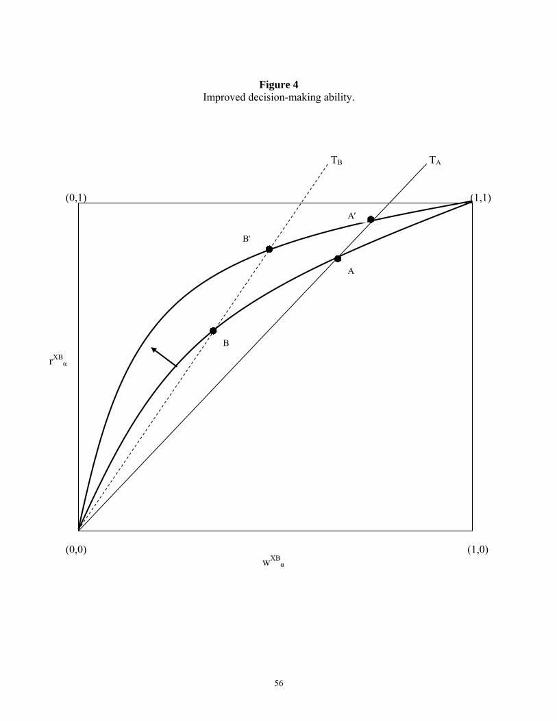
56

Figure 4

Improved decision-making ability. TB TA (0,1) (1,1)

rXBα (0,0) (1,0)

wXBα

A′

A

B′

B

57

Appendix Table A3 Corresponds to Table 3, but includes SPREAD on right-hand-side of regressions.

[1] [2] SCORER=AUTOAPP

[3] Discrete DISTANCE

Variable Coefficient p>Chi Sq. Coefficient p>Chi Sq. Coefficient p>Chi Sq.Intercept -6.9081 <.0001 -6.9446 <.0001 -6.8712 <.0001 SBA% 0.5633 0.0055 0.5198 0.0091 0.5773 0.0044 lnDISTANCE 0.0413 <.0001 0.0390 <.0001 DIST2550 0.1276 0.0206 DIST50UP 0.2622 <.0001 SCORER 0.3409 0.0003 0.2942 0.0265 0.2820 0.0001 SCORER*lnDISTANCE -0.0544 0.0184 -0.0572 0.0730 SCORER*DIST2550 -0.1415 0.3698 SCORER*50UP -0.3187 0.0023 SPREAD 0.1153 0.0067 0.1188 0.0051 0.1162 0.0063 MATURITY3 0.6195 <.0001 0.6164 <.0001 0.6229 <.0001 MATURITY7 0.6046 <.0001 0.6037 <.0001 0.6071 <.0001 FIRMSIZE 0.0003 0.0005 0.0003 0.0005 0.0003 0.0005 NEWFIRM 0.1959 <.0001 0.1984 <.0001 0.1954 <.0001 HHI 0.0336 0.8790 0.0389 0.8603 -0.0001 0.9995 HHI*URBAN -0.8361 0.0046 -0.8218 0.0053 -0.8630 0.0035 URBAN 0.1563 0.0561 0.1549 0.0581 0.1781 0.0293 CLP -0.1959 <.0001 -0.2006 <.0001 -0.1957 <.0001 PLP -0.3297 <.0001 -0.3293 <.0001 -0.3365 <.0001 BANKSIZE -0.0196 0.0288 -0.0133 0.1140 -0.0210 0.0187 RESERVES -0.0562 0.0041 -0.0580 0.0030 -0.0566 0.0038 CHARGEOFFS 6.3999 0.0006 6.5703 0.0004 6.4309 0.0005 INCOMEGROWTH -0.9512 0.0989 -0.9609 0.0956 -0.9524 0.0995 JOBGROWTH -4.2375 0.0009 -4.1615 0.0011 -4.2735 0.0009 POLICY9401 0.3185 <.0001 0.3289 <.0001 0.3166 <.0001 POLICYPOST89 -0.3703 <.0001 -0.3719 <.0001 -0.3661 <.0001 LOANAGE(4,5) 1.4850 <.0001 1.4847 <.0001 1.4850 <.0001 LOANAGE(6,7) 1.7037 <.0001 1.7031 <.0001 1.7036 <.0001 LOANAGE(8,9) 1.8043 <.0001 1.8037 <.0001 1.8043 <.0001 LOANAGE(10,12) 1.7527 <.0001 1.7519 <.0001 1.7527 <.0001 LOANAGE(13,15) 1.7034 <.0001 1.7018 <.0001 1.7034 <.0001 LOANAGE(16,20) 1.6204 <.0001 1.6176 <.0001 1.6197 <.0001 LOANAGE(21+) 1.3822 <.0001 1.3771 <.0001 1.3817 <.0001 Marginal effects: SBA% 0.00499 0.00460 0.00511 lnDISTANCE 0.00030 0.00031 DIST2550 0.00097 DIST50UP 0.00195 SCORER 0.00198 0.00151 0.00196 lnDISTANCE(SCORER=0) 0.00036 0.00034 lnDISTANCE(SCORER=1) -0.00014 -0.00019 DIST2550 (SCORER=0) 0.00109 DIST2550 (SCORER=1) -0.00016 DIST50UP (SCORER=0) 0.00225 DIST50UP (SCORER=1) -0.00063

58

Appendix Table A4a Corresponds to Table 4a, but includes SPREAD on right-hand-side of regressions.

[4]

Survey years only 1984 -1998

[5] First half

1984 -1992

[6] Second half 1993 -2001

[7] Second half 1993-2001

Variable Coefficient p>Chi Sq. Coefficient p>Chi Sq. Coefficient p>Chi Sq. Coefficient p>Chi Sq. SBA% 0.3219 0.1857 0.2526 0.5457 0.7998 0.0006 0.8801 0.0002 lnDISTANCE 0.0408 <.0001 0.0577 0.0003 0.0199 0.0643 0.0287 0.0197 SCORER 0.3755 0.0005 0.2981 0.0022 SCORER*lnDISTANCE -0.0489 0.0858 -0.0462 0.0560 SPREAD 0.0609 0.2492 -0.8236 <.0001 0.3854 <.0001 0.3833 <.0001 N 435,305 166,933 324,579 324,579 D=1 3,935 1,412 2,992 2,992 D=0 431,370 165,521 321,587 321,587 % SCORER=1 7.59% 0.00% 17.17% 17.27% Marginal effects: SBA% 0.00288 0.00211 0.00728 0.00801 lnDISTANCE 0.00032 0.00048 0.00018 0.00018 lnDISTANCE(SCORER=0) 0.00036 0.00026 lnDISTANCE(SCORER=1) -0.00009 -0.00019 SCORER 0.00246 0.00172

Appendix Table A4b

Corresponds to Table 4b, but includes SPREAD on right-hand-side of regressions.

[8] Loan ≤ $100,000

[9] Loan ≤ $250,000

[10] Loan > $100,000

Variable Coefficient p>Chi Sq. Coefficient p>Chi Sq. Coefficient p>Chi Sq. SBA% 0.8343 0.0014 0.7619 0.0007 -0.0353 0.9224 lnDISTANCE 0.0347 0.0056 0.0389 0.0002 0.0505 0.0010 SCORER 0.2269 0.0481 0.3319 0.0009 0.5860 0.0004 SCORER*lnDISTANCE -0.0257 0.3620 -0.0470 0.0554 -0.1070 0.0091 SPREAD 0.1453 0.0087 0.1201 0.0093 0.0667 0.3219 N 271,307 409,390 220,205 D=1 2,746 3,775 1,658 D=0 268,561 405,615 218,547 % SCORER=1 13.22% 12.11% 9.17% Marginal effects: SBA% 0.00833 0.00694 -0.00026 lnDISTANCE 0.00031 0.00030 0.00029 lnDISTANCE(SCORER=0) 0.00034 0.00035 0.00037 lnDISTANCE(SCORER=1) 0.00010 -0.00009 -0.00059 SCORER 0.00172 0.00211 0.00262

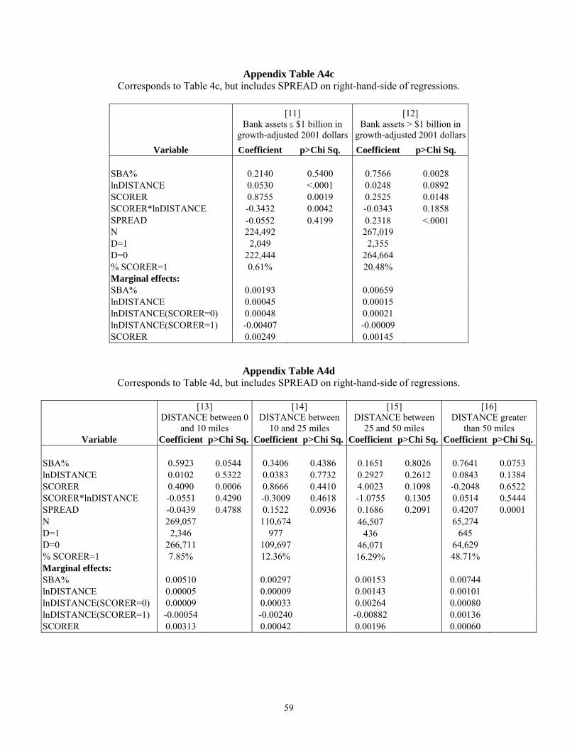
59

Appendix Table A4c Corresponds to Table 4c, but includes SPREAD on right-hand-side of regressions.

[11]

Bank assets ≤ $1 billion in growth-adjusted 2001 dollars

[12] Bank assets > $1 billion in

growth-adjusted 2001 dollarsVariable Coefficient p>Chi Sq. Coefficient p>Chi Sq.

SBA% 0.2140 0.5400 0.7566 0.0028 lnDISTANCE 0.0530 <.0001 0.0248 0.0892 SCORER 0.8755 0.0019 0.2525 0.0148 SCORER*lnDISTANCE -0.3432 0.0042 -0.0343 0.1858 SPREAD -0.0552 0.4199 0.2318 <.0001 N 224,492 267,019 D=1 2,049 2,355 D=0 222,444 264,664 % SCORER=1 0.61% 20.48% Marginal effects: SBA% 0.00193 0.00659 lnDISTANCE 0.00045 0.00015 lnDISTANCE(SCORER=0) 0.00048 0.00021 lnDISTANCE(SCORER=1) -0.00407 -0.00009 SCORER 0.00249 0.00145

Appendix Table A4d Corresponds to Table 4d, but includes SPREAD on right-hand-side of regressions.

[13]

DISTANCE between 0 and 10 miles

[14] DISTANCE between

10 and 25 miles

[15] DISTANCE between

25 and 50 miles

[16] DISTANCE greater

than 50 miles Variable Coefficient p>Chi Sq. Coefficient p>Chi Sq. Coefficient p>Chi Sq. Coefficient p>Chi Sq.

SBA% 0.5923 0.0544 0.3406 0.4386 0.1651 0.8026 0.7641 0.0753 lnDISTANCE 0.0102 0.5322 0.0383 0.7732 0.2927 0.2612 0.0843 0.1384 SCORER 0.4090 0.0006 0.8666 0.4410 4.0023 0.1098 -0.2048 0.6522 SCORER*lnDISTANCE -0.0551 0.4290 -0.3009 0.4618 -1.0755 0.1305 0.0514 0.5444 SPREAD -0.0439 0.4788 0.1522 0.0936 0.1686 0.2091 0.4207 0.0001 N 269,057 110,674 46,507 65,274 D=1 2,346 977 436 645 D=0 266,711 109,697 46,071 64,629 % SCORER=1 7.85% 12.36% 16.29% 48.71% Marginal effects: SBA% 0.00510 0.00297 0.00153 0.00744 lnDISTANCE 0.00005 0.00009 0.00143 0.00101 lnDISTANCE(SCORER=0) 0.00009 0.00033 0.00264 0.00080 lnDISTANCE(SCORER=1) -0.00054 -0.00240 -0.00882 0.00136 SCORER 0.00313 0.00042 0.00196 0.00060