container transport network for sustainable development in
TRANSCRIPT

sustainability
Article
Container Transport Network for SustainableDevelopment in South Korea
Kevin X. Li 1, Tae-Joon Park 2, Paul Tae-Woo Lee 3 , Heather McLaughlin 4 andWenming Shi 5,*
1 Ocean College, Zhejiang University, Zhoushan 316021, China; [email protected] Department of Business Administration, Yonsei University, Seoul 03722, South Korea; [email protected] Ocean College, Zhejiang University, Zhoushan 316021, China; [email protected] Faculty of Business and Law, Coventry University, Coventry CV1 5DL, UK; [email protected] Maritime and Logistics Management, Australian Maritime College, University of Tasmania,
Launceston TAS 7250, Australia* Correspondence: [email protected]; Tel.: +61-046-906-6614
Received: 16 July 2018; Accepted: 29 September 2018; Published: 7 October 2018�����������������
Abstract: The ever-increasing tendency toward economic globalization highlights the importanceof sustainable container transport networks to a country’s international trade, especially for aneconomy that is highly dependent on exports. This paper aims to develop a transport networkconnectivity index (TNCI) to measure the container transport connectivity from a multi-modalperspective. The proposed index is based on both graph theory and economics, considering transportinfrastructure and capacity, cargo flow, and capacity utilization. Using the case of South Korea asan example, we apply the TNCI to assess the connectivity of the Busan, Gwangyang, and Incheonports, representing approximately 96% of the container throughput in South Korea. The calculatedTNCI not only provides insight into the assessment of sustainable port competitiveness, it also helpspolicymakers identify bottlenecks in multi-modal transport networks. To eliminate these bottlenecks,this paper offers some appropriate measures and specific strategies for port development, which inturn improves the connectivity of container transport networks for sustainable development.
Keywords: sustainable container transport; multi-modal transport; graph theory; port managementinformation system; shipping policy
1. Introduction
The tendency toward economic globalization has emphasized world merchandise trade as well asinternational seaborne trade. According to the Review of Maritime Transport (2017) [1], the volumeof international seaborne trade has expanded significantly over the last four decades, rising from2.61 billion tons in 1970 to 4.01 billion tons in 1990, 8.41 billion tons in 2010, and 10.29 billion tons in 2016.Particularly, as shown in Table 1, container trade has also increased from 1001 million tons loaded in2005 to 1280 million tons loaded in 2010, reaching 1720 million tons loaded in 2016. The ever-increasingvolume of seaborne trade drives the demand for maritime transport services, especially for containertransport services [2]. When providing container transport services, ports play a substantial role as acluster of loading, unloading, and transshipment activities, shipbrokers, warehousing, and storageservices [3] (pp. 638–655), [4]. In this sense, connectivity between the port and its inland containertransport networks has a profound impact on port efficiency and port productivity, as well as on acountry’s exports and imports.
Sustainability 2018, 10, 3575; doi:10.3390/su10103575 www.mdpi.com/journal/sustainability

Sustainability 2018, 10, 3575 2 of 16
Table 1. Development of international seaborne trade (millions of tons loaded). Sources: Review ofMaritime Transport, 2017, UNCTAD (United Nations Conference on Trade and Development).
Year Oil and Gas Main Bulk Container Other Dry Cargo
2005 2422 1709 1001 29782006 2698 1814 1076 31882007 2747 1953 1193 33342008 2742 2065 1249 34222009 2642 2085 1127 31312010 2772 2335 1280 33022011 2794 2486 1393 35052012 2841 2742 1464 36142013 2829 2923 1544 37622014 2825 2985 1640 40332015 2932 3121 1661 39712016 3055 3172 1720 4059
When providing container transport services, better port connectivity with inland containertransport networks is more likely to reduce transit and transport time, and lower transport costs,thereby decreasing the risk of product damage and ensuring product quality. Meanwhile, productsunloaded at a port are likely to be delivered faster to customers, which can increase customersatisfaction with shippers, and consequently lead to positive word-of-mouth from satisfied customers.As a result, better port connectivity with inland container transport networks would enlarge a port’soverall captive area, and thereby enable it to serve larger hinterland markets [5]. This potentiallystrengthens a port’s efficiency and promotes port development in a sustainable manner. In addition,the local economy can also benefit when ports and inland container transport networks arewell-connected. For example, better connectivity usually indicates higher market reachability andaccessibility to goods and services, and then potentially reduces local firms’ logistics costs and facilitatestheir import and export business, shaping a sustainable and healthy economy [6]. Due to the decreasedlogistics costs, more foreign direct investments could be attracted to the local economy. In contrast,delivery delays and traffic congestions are more likely to occur when poor connectivity among roads,railways, and ports is observed. The congested container transport network can cause significantnegative impacts not only on port users and port authorities, but also on local environment andresidents [7]. Policymakers need to identify bottlenecks in multi-modal transport networks. By doingso, they can improve the efficiency of transport investments among roads, railways, and ports toachieve a better integration of sustainability in transporting containers. Using container transport inSouth Korea as a case study, this paper aims to develop a transport network connectivity index (TNCI)to examine how containers are transported from the multi-modal perspective. After consideringtransport infrastructure and capacity, cargo flow, and capacity utilization, the difference between thelink capacity and its cargo flow can be used to evaluate the container transport network connectivity,which enables port users to identify ports that have a better connection with inland containertransport networks.
Connectivity is a fundamental concept in graph theory. In a representative graph consisting ofnodes, arcs, and flows, a node is a connection point, a redistribution point, or a flow endpoint; an arc isa link between two different nodes reflecting costs, flow limits, or specific conditions; and flow showsthe quantity of an object movement, which is described by the sequence of a node and arc where flowpasses. Accordingly, connectivity can be defined as the minimum number of elements (nodes or edges)that need to be removed to disconnect the remaining nodes from each other [8] (p. 173). Since a graphand a transport network have a lot in common, graph theory has been widely applied in the fieldof transportation. Specifically, in a transport network, a node generally refers to the cargo-handlingfacility or origin/destination of cargo; an arc can be a road, railway, sea route, or airway that connectsnodes; and a flow usually represents the real cargo movement between two different regions. In this

Sustainability 2018, 10, 3575 3 of 16
regard, connectivity is redefined as the number of paths or maximum flow quantity between twodifferent nodes in this paper.
In the field of transportation, the air connectivity index (ACI) is a widely known connectivityindicator that seeks to measure the integration in the global air transport network. Using a generalizedgravity model, Arvis and Shepherd defined the ACI as the importance of a nation as a node withinthe global air transport system, and pointed out that the ACI was strongly correlated with the degreeof liberalization in air service markets [9]. Apart from the ACI, the liner shipping connectivity index(LSCI) developed by the United Nations Conference on Trade and Development (UNCTD) in 2007seeks to capture how well nations are connected to global shipping networks. Five componentsof the maritime transport sector involving the number of ships, their container-carrying capacity,maximum vessel size, number of services, and number of companies that deploy container shipsin a nation’s ports are included in the LSCI. Hoffman and Wilmsmeier identified the LSCI and portinfrastructure as important determinants of intra-Caribbean freight rates [10]. Additionally, the KOFSwiss Economic Institute published the globalization index to reflect global connectivity, integration,and interdependence in the economic, social, technological, cultural, political, and ecological spheres.A closer inspection of the economic globalization index reveals that two different types of dataare involved. One type represents actual flows regarding trade, foreign direct investment (FDI),portfolio investment, and income payments to foreign nationals. The other type represents restrictions,such as hidden import barriers, the mean tariff rate, taxes on international trade, and capital accountrestrictions [11].
Other popular applications of connectivity are as follows: transit connectivity measuringhow equitable the distribution of transit access is in a region [12,13], network connectivitypertaining to the issue of non-motorized transport and university populations [14], cultural heritageconnectivity regarding transportation infrastructure planning [15], city connectivity concerninginfrastructure networks among 67 important South Asian cities [16], and port connectivity in terms ofinter-port relationships from the perspective of a supply chain [17], its impact on the transportationnetwork [18,19], transport costs [20], transit time [21], and transportation access [22].
A more detailed discussion of port connectivity based on the graph theory can be found in [20].Focusing on degree, betweenness, and port accessibility index, they highlighted the crucial roleof port connectivity in keeping transport costs under control. Jiang et al. introduced two models,the minimum transportation time model and the maximum transportation capacity model, to measureport connectivity from a global container liner shipping network perspective [18]. Lam and Yap placedemphasis on shipping capacity, trade routes, and geographic regions, as well as on the extensity andintensity of inter-port relationships among ports [17]. Unlike the aforementioned studies, we focuson transport infrastructure and capacity, cargo flow, and capacity utilization, and derive the TNCI tomeasure container port connectivity from the multi-modal perspective, rather than from the inter-portperspective. The calculated TNCI not only provides insight into port competitiveness, but also helpspolicymakers to identify bottlenecks in multi-modal transport networks. After taking appropriatemeasures, these bottlenecks could be eliminated, which in turn can improve the connectivity ofcontainer transport networks in South Korea.
The remainder of this paper is structured as follows. Section 2 presents the potentialmethodological issues and derives the TNCI. Using the case of South Korea as an example, Section 3demonstrates data collection and parameter estimations. Section 4 gives a detailed discussion of SouthKorea’s container transport network connectivity. Finally, relevant conclusions and directions forfuture research are shown in Section 5.
2. Materials and Methods
Since the multi-modal transport network and the graph theory have a lot in common, it is widelyaccepted that a transport network can be represented as a graph, and then its connectivity can beexamined using the graph theory. Using container transport as an example, a node represents the

Sustainability 2018, 10, 3575 4 of 16
facility where a container is handled for transit, consolidation, or other specific purposes, while a linkdenotes the transport infrastructure that connects different nodes through roads/railways. Consideringthe capacity utilization rate and variance in cargo flow, we can compare the link capacity and the cargoflow to measure connectivity.
Specifically, when the link capacity is smaller than the cargo flow, it is generally believed thatroads/railways have been over-utilized, resulting in serious congestion. Then, poor connectivity canbe observed in the container transport network. On the other hand, when the link capacity is higherthan the cargo flow, the roads/railways have not been fully utilized; the larger the difference betweenthem, the lower the possibility of observing congestion. This can reduce the negative impacts of landtransport on environment and then promote the economy in a sustainable manner [23]. In other words,the container transport network is more likely to be well-connected, and better connectivity is likely tobe seen. In this regard, the difference between the link capacity and its cargo flow can be regarded as areasonable evaluation of connectivity, which can be used as a criterion for shipping lines’ port selection.
Before developing the TNCI, some parameters relevant to a multi-modal transport network aredefined as follows:
N set of nodesL set of links connecting two different nodesV(i,j) variance in cargo flow from node i to node j
U(i,j) capacity utilization ratio of link connecting node i and node j
F(i,j,t) cargo flow from node i to node j at time t
C(i,j,t) capacity of link connecting node i and node j
where t ∈ {c = current; f = f uture} and i, j ∈ N
First, V(i,j) is the variance in F(i,j,t) from node i to node j at time t, representing how far a set of cargoflows are spread out from their mean level over a given period. In general, frequent fluctuations incargo flows between different nodes are more likely to cause a higher variance, which pose challengesto transport infrastructure and require adaptations. Subsequently, a congestion problem is more likelyto occur due to the inappropriate provision of transport facilities and infrastructures. This, in turn,will negatively affect transport service providers and increase the transport time and transport costs.Let µ(i,j) be the mean of cargo flows from i to j over the given period, and then V(i,j) can be defined as:
V(i,j) = E[(
F(i,j,t) − µ(i,j)
)2]
(1)
However, the accurate calculation of variance is very difficult in reality. For the sake of simplicity,we consider formula (2) as an alternative since cargo flows between different nodes are usuallyunevenly distributed over the time of day. Let NTV be the nighttime traffic volume and DTV be thedaytime traffic volume. As a result, the calculated variance is 1.7522 for road cargo flow and is 2 forrailway cargo flow in the case study.
V = [NTV/(NTV + DTV)]−1 (2)
Second, U(i,j) is the capacity utilization rate of the link connecting two different nodes and isgenerally influenced by a variety of factors such as the accident ratio per mile and the number ofaccident-related deaths per registered vehicle or freight car. However, in practice, it is quite difficultto obtain an accurate U(i,j). We therefore consider the use of a proxy indicator. According to Changand Xiang, a higher U(i,j) often indicates a higher probability of accidents, because accidents are morelikely to occur in jammed or disordered situations [24]. This would reduce the overall utilization rateof the multi-modal transport network. In this sense, U(i,j) can be calculated as:
U(i,j) = NA/NR (3)

Sustainability 2018, 10, 3575 5 of 16
where NA is the total number of accidents, and NR is the total number of registered vehicles (or freightcars). Nevertheless, the capacity utilization rate of the link connecting two different nodes basedon Formula (3) is normally far below one, which generates an adjusted capacity that is close tozero. Meanwhile, the relation between cargo flow and capacity indicates that cargo flow can behigher or lower than capacity, which is affected by the utilization rate. Therefore, to avoid capacitydepletion, a revised Formula (4) is applied to calculate the overall capacity utilization rate of thelink [24]. As a result, the calculated capacity utilization rates are 1.0177 and 1.0714 for the railway androad, respectively.
U = 1 + NA/NR (4)
Third, with respect to C(i,j,t), the capacity of the link connecting two different nodes, current andfuture levels can be taken from government development plans, annual reports, and other guidelinesor news released to the public. Up to now, current cargo flow values can be calculated based oncontainer throughput, while their future values can be predicted using the autoregressive integratedmoving average (ARIMA) model [25,26].
Finally, the connectivity of container transport network can be developed according to thefollowing steps:
Step 1: For each pair of nodes (i, j), calculate the current and future values of cargo flow andcapacity F(i,j,t) and C(i,j,t), respectively.
Step 2: Calculate the total flow of cargo (F) transported to a port and the total capacity (C) as:
F = ∑(i,j∈N)
F(i,j,t) ×V(i,j); C = ∑(i,j∈N)
C(i,j,t) ×U(i,j) (5)
Step 3: Compute the difference between C and F, and then develop the TNCI:
TNCI = ∑(i,j∈N)
(C(i,j,t) ×U(i,j) − F(i,j,t) ×V(i,j)
)(6)
Note that choosing different values of t in Formula (6) will result in the current and future TNCIs.In the case study, Formula (7) is employed to consider that containers are transported to ports mainlyvia roads (99.5%) and railways (0.5%) in South Korea. Tables 3–5 offer more details.
TNCIGT,PMIS = C×(
0.995×Uroad + 0.005×Urailway
)− FGT,PMIS ×
(0.995×Vroad + 0.005×Vrailway
)(7)
Whether a specific transport mode is a bottleneck in the multi-modal transport network can bedetermined by examining the difference between capacity and cargo flow. After taking appropriatemeasures, the identified bottlenecks can be eliminated, which can improve the container transportnetwork connectivity.
To calculate the connectivity of the container transport network in South Korea, containerthroughput data in 2010 were collected from port authorities, while data on containers transportedvia roads and railways were obtained from the National Logistics Information Center, and otherrequired data were obtained from Statistics Korea. It should be mentioned here that road transportuses tonnage as units of container transport, while railway transport uses twenty-feet equivalent units(TEU). To ensure the consistency of measurement units, tonnage data were converted into TEU databy dividing by 18, because the transport regulations in South Korea limit the maximum weight of acontainer cargo trailer to 18 tons.
From the graph theory perspective, a node indicates a city or province in the container transportnetwork. As seen in Figure 1, 16 nodes were identified. Except for Jejudo (geographically isolatedfrom other regions, Jejudo has no railway lines; thus, we assume that there is only one cycle in Jejudo),each node has 56 arcs linking it to other nodes through roads and railways and one arc (the so-called

Sustainability 2018, 10, 3575 6 of 16
“cycle”) denotes container transport within this region. As a result, there are 856 arcs (consideringcontainer incoming and outgoing, each node is connected to 14 other nodes through roads and railways,and each node has a cycle. Thus, we have (14× 2× 2 + 1)× 15 + 1 = 856 arcs in total) in total. However,for simplicity, we excluded arcs with volumes below a certain level in this case study.Sustainability 2018, 10, x FOR PEER REVIEW 6 of 16
Figure 1. Administrative divisions of South Korea.
3. Results
3.1. Parameter Estimation
To calculate the TNCI, we first consider the current cargo flow by railway. The freeware
NodeXLGraph (https://nodexl.codeplex.com/) is used in this paper to represent the transport
network as a graph. An arc will be removed if the number of containers transported by this arc is
below 12, because regular service is defined as handling more than one container per month. With
the help of the maximum standardization method, values on arcs, divided by the maximum value
among all of the arcs, will lie between zero and one to reflect the number of containers handled
between two different regions (Appendix A). As demonstrated in Figure 2, the size of each node is
proportional to the total number of incoming and outgoing containers in this region. The width and
direction of an arc reflect the number of containers handled from origin to destination.
Second, the current cargo flow by road can be analyzed in a similar way. However, in a graph
representing the road container transport network, an arc with a cargo handling capacity below
10,000 TEU per month is removed. In general, Korean logistics companies provide more than 10,000
TEU line schedules per month between regions. In other words, when the cargo-handling capacity is
below 10,000 TEU per month (Jejudo is not connected to other regions via roads or railways and it
has a cycle of 72,047 TEU; it is thus not considered in the TNCI calculation because of its unique
geographical location.), it is considered a non-regular service. The network is displayed in Figure 3.
After comparing figures 2 and 3, it can be clearly seen that the arc distribution in the road network is
thicker and more balanced than that in the railway network (Appendix B). This is because the road
network has better accessibility, reachability, and capacity in South Korea, and thus it is more
frequently utilized.
Third, with respect to capacity, calculations of road and railway capacity are quite challenging
in civil engineering, because there are too many variables influencing the road and railway conditions
[27]. Although some indicators, such as road or railway length, lane number, and type (express or
Figure 1. Administrative divisions of South Korea.
3. Results
3.1. Parameter Estimation
To calculate the TNCI, we first consider the current cargo flow by railway. The freewareNodeXLGraph (https://nodexl.codeplex.com/) is used in this paper to represent the transport networkas a graph. An arc will be removed if the number of containers transported by this arc is below 12,because regular service is defined as handling more than one container per month. With the help of themaximum standardization method, values on arcs, divided by the maximum value among all of thearcs, will lie between zero and one to reflect the number of containers handled between two differentregions (Appendix A). As demonstrated in Figure 2, the size of each node is proportional to the totalnumber of incoming and outgoing containers in this region. The width and direction of an arc reflectthe number of containers handled from origin to destination.
Second, the current cargo flow by road can be analyzed in a similar way. However, in a graphrepresenting the road container transport network, an arc with a cargo handling capacity below 10,000TEU per month is removed. In general, Korean logistics companies provide more than 10,000 TEU lineschedules per month between regions. In other words, when the cargo-handling capacity is below10,000 TEU per month (Jejudo is not connected to other regions via roads or railways and it has a cycleof 72,047 TEU; it is thus not considered in the TNCI calculation because of its unique geographicallocation.), it is considered a non-regular service. The network is displayed in Figure 3. After comparing

Sustainability 2018, 10, 3575 7 of 16
Figures 2 and 3, it can be clearly seen that the arc distribution in the road network is thicker and morebalanced than that in the railway network (Appendix B). This is because the road network has betteraccessibility, reachability, and capacity in South Korea, and thus it is more frequently utilized.
Sustainability 2018, 10, x FOR PEER REVIEW 7 of 16
non-express), can reflect road or railway capacity, it is hard to synthesize these data to obtain a
comprehensive capacity indicator. To address this problem, the concept of source and sink in the
graph theory is applied [6] (p.173), [28]. In a directed graph, (a directed graph is a finite set of nodes,
some of which are connected by arrows. In graph theory, a flow network, which is also known as a
transportation network, is a directed graph where each edge has a capacity, and each edge receives
flow. The amount of flow cannot exceed its capacity (https://en.wikipedia.org/wiki/Flow_network, a
source is a node such that the arrows touching the node point away from the node, while a sink is a
node such that all of the arrows touching the node point into the node. Likewise, in a transport
network, a source generates flow, while a sink receives flow. Moreover, the flow in the network must
arrive at the destination. Otherwise, the network will become jammed by overloading. When using
containers for export, they are generally transported to ports via roads, railways, or inland
waterways, and then they are transported to their destination ports by maritime transport.
Meanwhile, when using containers for import, containers arriving at ports by maritime transport will
be delivered all over the country by inland transport. In this sense, a port acts as both a source and a
sink in container transport networks.
Figure 2. The current railway cargo flow. Sources: Authors. Figure 2. The current railway cargo flow. Sources: Authors.
Third, with respect to capacity, calculations of road and railway capacity are quite challenging incivil engineering, because there are too many variables influencing the road and railway conditions [27].Although some indicators, such as road or railway length, lane number, and type (express ornon-express), can reflect road or railway capacity, it is hard to synthesize these data to obtain acomprehensive capacity indicator. To address this problem, the concept of source and sink in thegraph theory is applied [6] (p. 173), [28]. In a directed graph, (a directed graph is a finite set of nodes,some of which are connected by arrows. In graph theory, a flow network, which is also known as atransportation network, is a directed graph where each edge has a capacity, and each edge receivesflow. The amount of flow cannot exceed its capacity (https://en.wikipedia.org/wiki/Flow_network,a source is a node such that the arrows touching the node point away from the node, while a sinkis a node such that all of the arrows touching the node point into the node. Likewise, in a transportnetwork, a source generates flow, while a sink receives flow. Moreover, the flow in the network mustarrive at the destination. Otherwise, the network will become jammed by overloading. When usingcontainers for export, they are generally transported to ports via roads, railways, or inland waterways,and then they are transported to their destination ports by maritime transport. Meanwhile, when usingcontainers for import, containers arriving at ports by maritime transport will be delivered all overthe country by inland transport. In this sense, a port acts as both a source and a sink in containertransport networks.

Sustainability 2018, 10, 3575 8 of 16Sustainability 2018, 10, x FOR PEER REVIEW 8 of 16
Figure 3. The current cargo road cargo flow. Sources: Authors.
In the case of South Korea, we consider the Busan, Gwangyang, and Incheon ports, because these
ports accounted for roughly 96% of the total container port throughput in 2010 (see Table 2). In reality,
the port capacity is usually calculated based on the container volume handled per year at the port.
Table 3 shows the capacity information provided by port authorities. From Table 3, capacities were
13,865,000 TEU, 4,600,000 TEU, and 1,120,000 TEU for the Busan, Gwangyang, and Incheon ports in
2010, respectively.
Table 2. Container throughput of main ports in South Korea in 2010 (1000 TEU).
2007 2008 2009 2010 2011 2012 2013 2014
Busan 13,261 13,453 11,980 14,194 16,185 17,046 17,686 18,683
Gwangyang 1723 1810 1810 2073 2073 2154 2285 2338
Incheon 1664 1703 1578 1903 1998 1982 2161 2335
Others 699 757 697 783 856 890 905 938
% Top 3 96 96 96 96 96 96 96 96
Notes: Other includes the Pyeongtak and Ulsan ports. % Top 3 = 100×he container throughput of
Busan, Gwangyang, and Incheon/Total container throughput of all the international trade ports in
South Korea. Sources: Port authorities, The National Logistics Center, and Statistics Korea.
Figure 3. The current cargo road cargo flow. Sources: Authors.
In the case of South Korea, we consider the Busan, Gwangyang, and Incheon ports, because theseports accounted for roughly 96% of the total container port throughput in 2010 (see Table 2). In reality,the port capacity is usually calculated based on the container volume handled per year at the port.Table 3 shows the capacity information provided by port authorities. From Table 3, capacities were13,865,000 TEU, 4,600,000 TEU, and 1,120,000 TEU for the Busan, Gwangyang, and Incheon ports in2010, respectively.
Table 2. Container throughput of main ports in South Korea in 2010 (1000 TEU).
2007 2008 2009 2010 2011 2012 2013 2014
Busan 13,261 13,453 11,980 14,194 16,185 17,046 17,686 18,683Gwangyang 1723 1810 1810 2073 2073 2154 2285 2338
Incheon 1664 1703 1578 1903 1998 1982 2161 2335Others 699 757 697 783 856 890 905 938
% Top 3 96 96 96 96 96 96 96 96
Notes: Other includes the Pyeongtak and Ulsan ports. % Top 3 = 100×he container throughput of Busan, Gwangyang,and Incheon/Total container throughput of all the international trade ports in South Korea. Sources: Port authorities,The National Logistics Center, and Statistics Korea.

Sustainability 2018, 10, 3575 9 of 16
Table 3. Capacity of the Busan, Gwangyang, and Incheon ports in 2010 (1000 TEU).
Capacity Number of Terminal
Busan 13,865 9Gwangyang 4600 4
Incheon 1120 6Total 19,585 19
Notes: The Busan container port has nine terminals (e.g., Jasungdae, Shinsundae, Gamman, Shin Gamman, Uam,Pusan New Port International Terminal, Pusan New Port Terminal, Hanjin New Port Terminal, and Hyundai PusanNew-port Terminal), the Gwangyang port has four sub-terminals, and the Incheon port has six sub-terminals,respectively. Regarding the Gwangyang port, container and bulk cargo are separated when calculating the transportnetwork connectivity index (TNCI). Sources: Port authorities, The National Logistics Center, and Statistics Korea.
3.2. Calculation of the Connectivity Index
After estimating the required parameters, we move on to calculate the connectivity of the containertransport networks in South Korea. As previously discussed, the Busan, Gwangyang, and Incheonports can be seen as both sinks and sources. The TNCI can be calculated for each port to reflectits container transport network connectivity. Table 4 reports the calculated incoming, outgoing,and cycle containers based on graph theory. As reported in Table 4, the container throughputs were2,296,000 TEU, 5,192,000 TEU, and 14,136,000 TEU for the Gwangyang, Incheon, and Busan ports,respectively. To facilitate the daily operation of a port by giving users the information, notifications,and analysis that they need, port management information systems (PMISs) have been widely usedaround the world. As seen in Table 5, the container throughputs based on the PMIS were 2,088,000 TEU,1,902,000 TEU, and 14,113,000 TEU for the Gwangyang, Incheon, and Busan ports, respectively.The capacity of each port provided by port authorities is also given in Table 5. Then, the containerthroughput differences between the graph theory approach and the PMIS approach are larger in thecases of the Gwangyang and Incheon ports. A possible explanation lies in the type of cargo that ishandled at each port. For example, the large percentage of dry bulk that is handled at the Gwangyangand the Incheon ports has to be transformed into TEU units for comparison, which could magnify thecargo flow.
Table 4. Container throughput of the main ports based on graph theory (1000 TEU).
Gwangyang Incheon Busan
Incoming 386 1123 7886Outgoing 490 2284 3737
Cycle 1420 1785 2513Total 2296 5192 14,136
Notes: Cycle indicates the transshipment of containers within or near a port. Total indicates the calculated containerthroughput. Sources: Port authorities, The National Logistics Center, and Statistics Korea.
Table 5. Summary of container throughput of the main ports (1000 TEU). PMIS: port managementinformation systems.
Gwangyang Incheon Busan
Graph theory (GT) based 2296 5192 14,136PMIS based 2088 1902 14,113Capacity (C) 4600 1120 13,865
C-GT 2304 −4072 −271C-PMIS 2512 −782 −248
Sources: Authors.
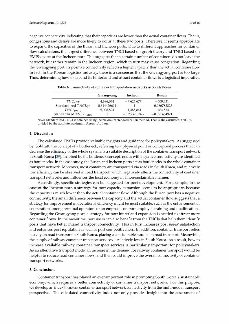
Using Formula (7), we obtain the needed TNCIs and report them in Table 6. As revealed by thestandardized TNCIs, in both cases, the Gwangyang port has the best connectivity, followed by theBusan port, and then the Incheon port. Specifically, the Busan and Incheon ports are found to have
Sustainability 2018, 10, 3575 10 of 16
negative connectivity, indicating that their capacities are lower than the actual container flows. That is,congestions and delays are more likely to occur at these two ports. Therefore, it seems appropriateto expand the capacities of the Busan and Incheon ports. Due to different approaches for containerflow calculations, the largest difference between TNCI based on graph theory and TNCI based onPMISs exists at the Incheon port. This suggests that a certain number of containers do not leave thenetwork, but rather remain in the Incheon region, which in turn may cause congestion. Regardingthe Gwangyang port, its positive connectivity reflects a higher capacity than the actual container flow.In fact, in the Korean logistics industry, there is a consensus that the Gwangyang port is too large.Thus, determining how to expand its hinterland and attract container flows is a logistical imperative.
Table 6. Connectivity of container transportation networks in South Korea.
Gwangyang Incheon Busan
TNCIGT 4,686,034 −7,626,677 −509,331Standardized TNCIGT 0.614426694 −1 −0.066782825
TNCIPMIS 5,078,824 −1,465,841 −464,534Standardized TNCIPMIS 1 −0.288618363 −0.091464971
Notes: Standardized TNCI is obtained using the maximum standardization method. That is, the calculated TNCI isdivided by the absolute maximum. Sources: Authors.
4. Discussion
The calculated TNCIs provide valuable insights and guidance for policymakers. As suggestedby Goldratt, the concept of a bottleneck, referring to a physical point or conceptual process that candecrease the efficiency of the whole system, is a suitable description of the container transport networkin South Korea [29]. Inspired by the bottleneck concept, nodes with negative connectivity are identifiedas bottlenecks. In the case study, the Busan and Incheon ports act as bottlenecks in the whole containertransport network. Moreover, most containers are transported via roads in South Korea, and relativelylow efficiency can be observed in road transport, which negatively affects the connectivity of containertransport networks and influences the local economy in a non-sustainable manner.
Accordingly, specific strategies can be suggested for port development. For example, in thecase of the Incheon port, a strategy for port capacity expansion seems to be appropriate, becausethe capacity is much lower than the actual container flow. Although the Busan port has a negativeconnectivity, the small difference between the capacity and the actual container flow suggests that astrategy for improvement in operational efficiency might be most suitable, such as the enhancement ofcooperation among terminal operators or an emphasis on port employee training and qualifications.Regarding the Gwangyang port, a strategy for port hinterland expansion is needed to attract morecontainer flows. In the meantime, port users can also benefit from the TNCIs that help them identifyports that have better inland transport connectivity. This in turn increases port users’ satisfactionand enhances port reputation as well as port competitiveness. In addition, container transport reliesheavily on road transport in South Korea, placing a considerable burden on road transport. Meanwhile,the supply of railway container transport services is relatively low in South Korea. As a result, how toincrease available railway container transport services is particularly important for policymakers.As an alternative transport mode, an increase in the demand for railway container transport would behelpful to reduce road container flows, and then could improve the overall connectivity of containertransport networks.
5. Conclusions
Container transport has played an ever-important role in promoting South Korea’s sustainableeconomy, which requires a better connectivity of container transport networks. For this purpose,we develop an index to assess container transport network connectivity from the multi-modal transportperspective. The calculated connectivity index not only provides insight into the assessment of
Sustainability 2018, 10, 3575 11 of 16
sustainable port competitiveness, it also helps policymakers identify bottlenecks in multi-modaltransport networks. Specifically, from the congestion perspective, a well-connected port usuallyindicates that the capacity is higher than the usage of links. The lower the difference, the higher thepossibility of observing congestion in container transport networks. This potentially reduces portattractiveness and moves shipping lines to call at other ports. In this sense, the connectivity index canbe used as a criterion for shipping lines’ port selection. On the other hand, the probability of congestionbecomes higher when the cargoes that are handled in a port are higher than the capacity, which usuallyindicates that the links are over-utilized. This also reflects that the container transport network isnot well-connected because of insufficient capacity, which in turn motivates capacity investment.In this regard, the developed connectivity index can also be used as a criterion for policymakers’investment decisions.
Using container transport in South Korea as a case study, some specific strategies are proposed toimprove port operations. For the Incheon port, it is suggested that port capacity needs to be expandedto facilitate the increasing container flows, resulting in the lower possibility of observing congestionsand delays. For the Busan port, more emphasis should be placed on improvements in operationalefficiency by effectively cooperating with terminal operators and training port employees. For theGwangyang port, the recommendation is to expand its hinterland and attract more container flows.At the same time, the bottleneck analysis also provides valuable insight and guidance for port userswho would benefit from identifying ports with superior container transport network connectivity.In addition, expanding the supply of railway container transport services in South Korea could reduceits heavy reliance on road transport.
Nevertheless, some potential limitations still exist in the current paper. For example, we onlyconsider connectivity for a single year, which may not enable us to explore the evolution of connectivityin container transport networks over time or model the future connectivity. Another limitation isthe potential underestimation of the road container cargo flow when using the maximum weight ofa container cargo trailer to convert the tonnage data. However, these limitations do present a newperspective and avenue for our future research.
Author Contributions: Conceptualization, K.X.L., T.-J.P. and W.S.; Methodology, T.-J.P. and W.S.; Software, T.-J.P.;Validation, P.T.-W.L. and H.M.; Formal Analysis, T.-J.P. and W.S.; Investigation, K.X.L., P.T.-W.L. and H.M.;Resources, T.-J.P.; Data Curation, T.-J.P.; Writing-Original Draft Preparation, T.-J.P. and W.S.; Writing-Review &Editing, K.X.L.; Visualization, P.T.-W.L. and H.M.; Supervision, K.X.L. and W.S.; Project Administration, K.X.L.
Funding: This research received no external funding.
Conflicts of Interest: The authors declare no conflict of interest.
Sustainability 2018, 10, 3575 12 of 16
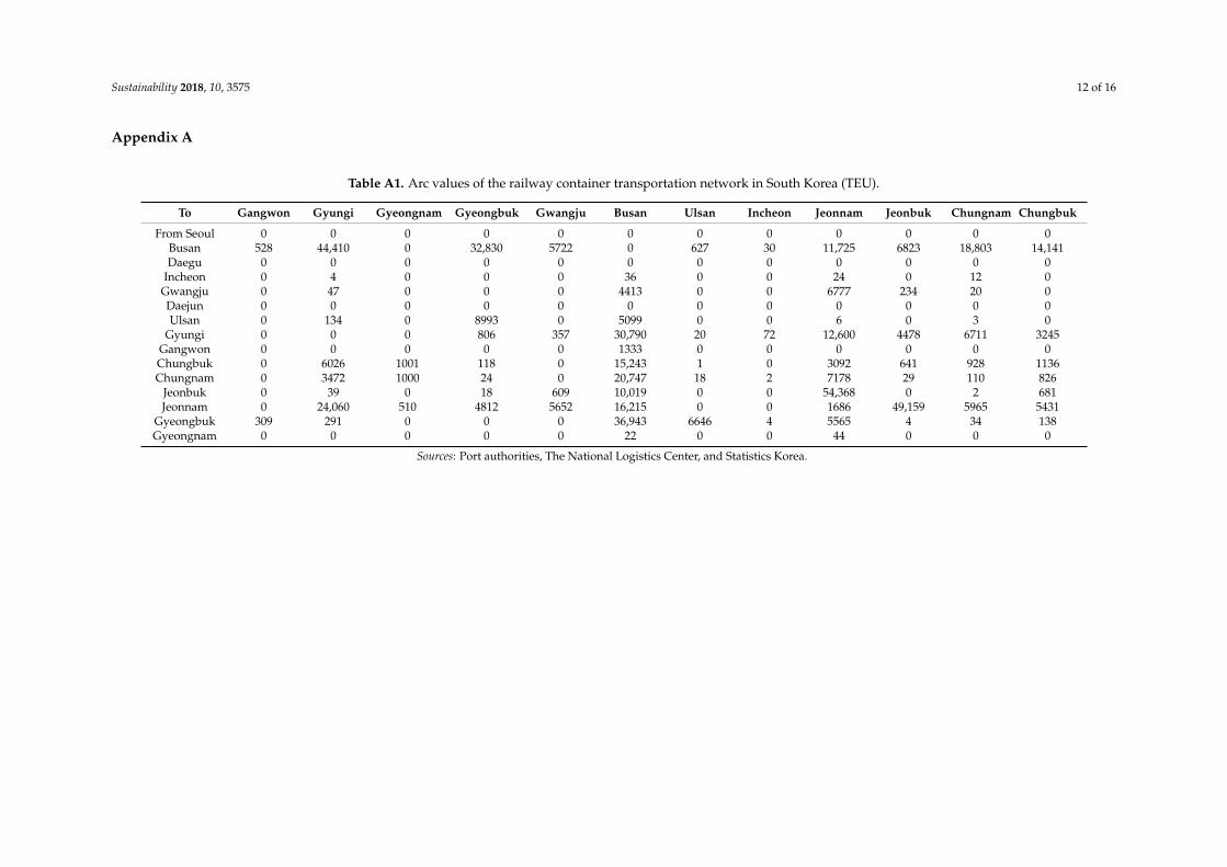
Appendix A
Table A1. Arc values of the railway container transportation network in South Korea (TEU).
To Gangwon Gyungi Gyeongnam Gyeongbuk Gwangju Busan Ulsan Incheon Jeonnam Jeonbuk Chungnam Chungbuk
From Seoul 0 0 0 0 0 0 0 0 0 0 0 0Busan 528 44,410 0 32,830 5722 0 627 30 11,725 6823 18,803 14,141Daegu 0 0 0 0 0 0 0 0 0 0 0 0
Incheon 0 4 0 0 0 36 0 0 24 0 12 0Gwangju 0 47 0 0 0 4413 0 0 6777 234 20 0Daejun 0 0 0 0 0 0 0 0 0 0 0 0Ulsan 0 134 0 8993 0 5099 0 0 6 0 3 0
Gyungi 0 0 0 806 357 30,790 20 72 12,600 4478 6711 3245Gangwon 0 0 0 0 0 1333 0 0 0 0 0 0Chungbuk 0 6026 1001 118 0 15,243 1 0 3092 641 928 1136Chungnam 0 3472 1000 24 0 20,747 18 2 7178 29 110 826
Jeonbuk 0 39 0 18 609 10,019 0 0 54,368 0 2 681Jeonnam 0 24,060 510 4812 5652 16,215 0 0 1686 49,159 5965 5431
Gyeongbuk 309 291 0 0 0 36,943 6646 4 5565 4 34 138Gyeongnam 0 0 0 0 0 22 0 0 44 0 0 0
Sources: Port authorities, The National Logistics Center, and Statistics Korea.

Sustainability 2018, 10, 3575 13 of 16
Appendix B
Table A2. Arc values of the road container transportation network in South Korea (TEU).
To Seoul Busan Daegu Incheon Gwangju Daejun Ulsan Gyungi Gangwon Chungbuk Chungnam Jeonbuk Jeonnam Gyeongbuk Gyeongnam
From Seoul 2,350,329 89,787 2708 336,403 1951 19,709 22,947 1,111,748 50,306 39,599 83,187 9051 10,392 7485 3746Busan 147,022 2,513,435 168,715 64,377 45,589 33,349 395,028 491,555 8738 106,332 124,008 93,698 92,769 495,698 1,334,919Daegu 12,526 178,332 722,271 3971 12,598 32,100 46,331 15,145 7147 32,856 21,911 27,955 18,831 374,277 207,934
Incheon 1,387,564 99,712 10,211 3,419,471 3176 27,706 8831 2,347,380 58,981 82,233 248,102 15,448 14,892 22,885 48,069Gwangju 6901 130,746 5618 1357 373,325 13,904 553 6156 361 5207 12,872 67,781 295,619 4374 18,952Daejun 32,577 51,462 10,827 4610 6785 233,730 786 32,551 3932 67,942 65,152 47,436 15,661 16,986 6941Ulsan 31,193 2,117,696 199,047 2646 11,729 18,156 3,818,570 53,042 13,349 25,616 48,687 22,429 48,260 423,677 880,629
Gyungi 3,390,682 504,339 15,394 1,289,431 9153 129,154 64,676 4,518,351 340,024 332,779 1,036,782 151,315 99,286 79,782 20,555Gangwon 126,908 21,467 19,584 29,838 545 15,294 4581 216,160 2,316,112 176,307 70,435 7218 2394 167,301 8940Chungbuk 221,506 93,735 48,384 41,334 9915 305,613 4672 311,151 163,131 634,277 403,875 77,694 31,765 187,757 50,220Chungnam 400,235 212,339 38,066 238,951 42,037 371,458 68,990 911,092 133,815 490,061 4,867,992 445,558 129,090 181,834 133,814
Jeonbuk 90,005 149,466 29,190 20,251 214,841 177,097 6615 81,697 8968 89,960 427,670 1,553,702 394,135 53,563 89,662Jeonnam 46,556 236,925 22,208 9450 616,446 19,955 26,719 76,534 4784 40,370 121,154 372,709 6,219,892 42,804 400,574
Gyeongbuk 95,983 944,981 937,104 95,165 17,790 118,332 374,247 83,123 132,688 228,287 167,701 72,472 54,291 4,330,971 553,570Gyeongnam 47,704 2,914,258 410,766 13,750 82,571 38,764 411,662 43,517 15,420 44,909 171,912 181,828 384,976 634,232 6,506,301
Sources: Port authorities, The National Logistics Center, and Statistics Korea. Jeju has cycle 72,047 TEU.
Appendix C
Table A3. Incoming and outgoing containers of the Busan port (1000 TEU).
Seoul Busan Daegu Incheon Gwangju Daejun Ulsan Gyungi Gangwon Chungbuk Chungnam Jeonbuk Jeonnam Gyeongbuk Gyeongnam Total
Outgoing 892513
178 99 135 51 2122 535 22 108 233 159 253 981 2914Incoming 147 168 64 51 33 395 535 9 120 142 100 104 528 1334
Total 236 2513 347 164 186 84 2518 1071 32 229 375 260 357 1510 4249 14,136% Total 2% 18% 2% 1% 1% 1% 18% 8% 0% 2% 3% 2% 3% 11% 30% 100%

Sustainability 2018, 10, 3575 14 of 16
Appendix D
Table A4. Incoming and outgoing containers of the Gwangyang port (1000 TEU).
Seoul Busan Daegu Incheon Gwangju Daejun Ulsan Gyungi Gangwon Chungbuk Chungnam Jeonbuk Jeonnam Gyeongbuk Gyeongnam Total
Incoming 3 1334 207 48 18 6 880 20 8 51 134 89 553 6506 0Outgoing 47 2914 410 13 82 38 411 43 15 44 171 181 6221 634
Total 51 4249 618 61 101 45 1292 64 24 96 306 271 6221 1187 6506 21,099% Total 0% 20% 3% 0% 0% 0% 6% 0% 0% 0% 1% 1% 29% 6% 31% 100%
Appendix E
Table A5. Incoming and outgoing containers of the Incheon port (1000TEU).
Seoul Busan Incheon Daegu Gwangju Daejun Ulsan Gyungi Gangwon Chungbuk Chungnam Jeonbuk Jeonnam Gyeongbuk Gyeongnam Total
Incoming 336 64 3419 3 1 4 2 1289 29 41 238 20 9 95 13 1808Outgoing 1387 99 10 3 27 8 2347 58 82 248 15 14 22 48 4358
Total 1723 164 3419 14 4 32 11 3636 88 123 487 35 24 118 61 9946% Total 17% 2% 34% 0% 0% 0% 0% 37% 1% 1% 5% 0% 0% 1% 1% 100%
Sources: Port authorities, The National Logistics Center, and Statistics Korea. Total=incoming + outgoing + cycle.
Sustainability 2018, 10, 3575 15 of 16
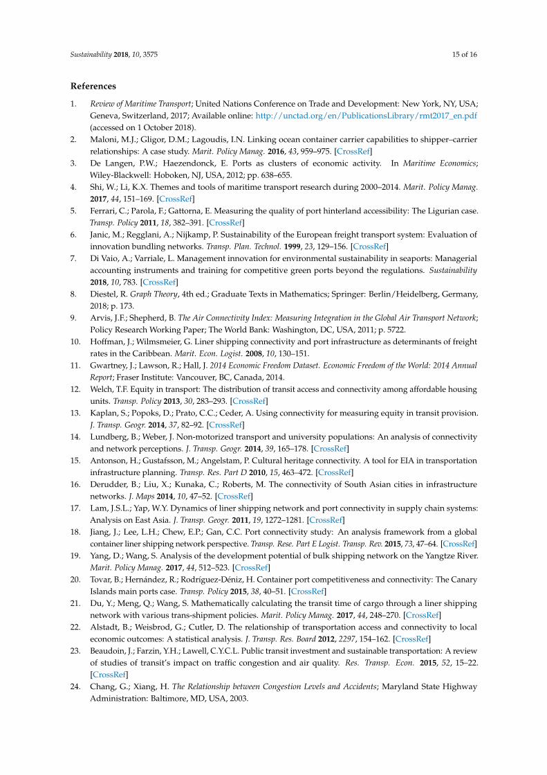
References
1. Review of Maritime Transport; United Nations Conference on Trade and Development: New York, NY, USA;Geneva, Switzerland, 2017; Available online: http://unctad.org/en/PublicationsLibrary/rmt2017_en.pdf(accessed on 1 October 2018).
2. Maloni, M.J.; Gligor, D.M.; Lagoudis, I.N. Linking ocean container carrier capabilities to shipper–carrierrelationships: A case study. Marit. Policy Manag. 2016, 43, 959–975. [CrossRef]
3. De Langen, P.W.; Haezendonck, E. Ports as clusters of economic activity. In Maritime Economics;Wiley-Blackwell: Hoboken, NJ, USA, 2012; pp. 638–655.
4. Shi, W.; Li, K.X. Themes and tools of maritime transport research during 2000–2014. Marit. Policy Manag.2017, 44, 151–169. [CrossRef]
5. Ferrari, C.; Parola, F.; Gattorna, E. Measuring the quality of port hinterland accessibility: The Ligurian case.Transp. Policy 2011, 18, 382–391. [CrossRef]
6. Janic, M.; Regglani, A.; Nijkamp, P. Sustainability of the European freight transport system: Evaluation ofinnovation bundling networks. Transp. Plan. Technol. 1999, 23, 129–156. [CrossRef]
7. Di Vaio, A.; Varriale, L. Management innovation for environmental sustainability in seaports: Managerialaccounting instruments and training for competitive green ports beyond the regulations. Sustainability2018, 10, 783. [CrossRef]
8. Diestel, R. Graph Theory, 4th ed.; Graduate Texts in Mathematics; Springer: Berlin/Heidelberg, Germany,2018; p. 173.
9. Arvis, J.F.; Shepherd, B. The Air Connectivity Index: Measuring Integration in the Global Air Transport Network;Policy Research Working Paper; The World Bank: Washington, DC, USA, 2011; p. 5722.
10. Hoffman, J.; Wilmsmeier, G. Liner shipping connectivity and port infrastructure as determinants of freightrates in the Caribbean. Marit. Econ. Logist. 2008, 10, 130–151.
11. Gwartney, J.; Lawson, R.; Hall, J. 2014 Economic Freedom Dataset. Economic Freedom of the World: 2014 AnnualReport; Fraser Institute: Vancouver, BC, Canada, 2014.
12. Welch, T.F. Equity in transport: The distribution of transit access and connectivity among affordable housingunits. Transp. Policy 2013, 30, 283–293. [CrossRef]
13. Kaplan, S.; Popoks, D.; Prato, C.C.; Ceder, A. Using connectivity for measuring equity in transit provision.J. Transp. Geogr. 2014, 37, 82–92. [CrossRef]
14. Lundberg, B.; Weber, J. Non-motorized transport and university populations: An analysis of connectivityand network perceptions. J. Transp. Geogr. 2014, 39, 165–178. [CrossRef]
15. Antonson, H.; Gustafsson, M.; Angelstam, P. Cultural heritage connectivity. A tool for EIA in transportationinfrastructure planning. Transp. Res. Part D 2010, 15, 463–472. [CrossRef]
16. Derudder, B.; Liu, X.; Kunaka, C.; Roberts, M. The connectivity of South Asian cities in infrastructurenetworks. J. Maps 2014, 10, 47–52. [CrossRef]
17. Lam, J.S.L.; Yap, W.Y. Dynamics of liner shipping network and port connectivity in supply chain systems:Analysis on East Asia. J. Transp. Geogr. 2011, 19, 1272–1281. [CrossRef]
18. Jiang, J.; Lee, L.H.; Chew, E.P.; Gan, C.C. Port connectivity study: An analysis framework from a globalcontainer liner shipping network perspective. Transp. Rese. Part E Logist. Transp. Rev. 2015, 73, 47–64. [CrossRef]
19. Yang, D.; Wang, S. Analysis of the development potential of bulk shipping network on the Yangtze River.Marit. Policy Manag. 2017, 44, 512–523. [CrossRef]
20. Tovar, B.; Hernández, R.; Rodríguez-Déniz, H. Container port competitiveness and connectivity: The CanaryIslands main ports case. Transp. Policy 2015, 38, 40–51. [CrossRef]
21. Du, Y.; Meng, Q.; Wang, S. Mathematically calculating the transit time of cargo through a liner shippingnetwork with various trans-shipment policies. Marit. Policy Manag. 2017, 44, 248–270. [CrossRef]
22. Alstadt, B.; Weisbrod, G.; Cutler, D. The relationship of transportation access and connectivity to localeconomic outcomes: A statistical analysis. J. Transp. Res. Board 2012, 2297, 154–162. [CrossRef]
23. Beaudoin, J.; Farzin, Y.H.; Lawell, C.Y.C.L. Public transit investment and sustainable transportation: A reviewof studies of transit’s impact on traffic congestion and air quality. Res. Transp. Econ. 2015, 52, 15–22.[CrossRef]
24. Chang, G.; Xiang, H. The Relationship between Congestion Levels and Accidents; Maryland State HighwayAdministration: Baltimore, MD, USA, 2003.

Sustainability 2018, 10, 3575 16 of 16
25. Kim, C.B. Estimating and forecasting the trading volumes of airway transport. Air Transp. J. 2007, 10, 78–99.26. Peng, W.Y.; Chu, C.W. A comparison of univariate methods for forecasting container throughput volumes.
Math. Comput. Model. 2009, 50, 1045–1057. [CrossRef]27. Garber, N.; Hoel, L. Traffic and Highway Engineering; Cengage Learning: Boston, MA, USA, 2014.28. Gibbons, A. Algorithmic Graph Theory; Cambridge University Press: Cambridge, UK, 1985.29. Goldratt, E.M. Theory of Constraints; North River: Croton-on-Hudson, NY, USA, 1990.
© 2018 by the authors. Licensee MDPI, Basel, Switzerland. This article is an open accessarticle distributed under the terms and conditions of the Creative Commons Attribution(CC BY) license (http://creativecommons.org/licenses/by/4.0/).