constraint generation for two-stage robust network flow ... · pdf fileconstraint generation...
TRANSCRIPT

Constraint Generation for Two-Stage RobustNetwork Flow Problem
David Simchi-LeviDepartment of Civil and Environmental Engineering, Institute for Data, Systems and Society, Operations Research Center,
Massachusetts Institute of Technology, [email protected]
He WangSchool of Industrial and Systems Engineering, Georgia Institute of Technology, [email protected]
Yehua WeiCarroll School of Management, Boston College, [email protected]
In this paper, we propose new constraint generation algorithms for solving the two-stage robust minimum
cost flow problem, a problem that arises from various applications such as transportation and logistics. In
order to develop efficient algorithms under general polyhedral uncertainty set, we repeatedly exploit the
network-flow structure to reformulate the two-stage robust minimum cost flow problem as a single-stage
optimization problem. The reformulation gives rise to a natural constraint generation (CG) algorithm, and
more importantly, leads to a method for solving the separation problem using a pair of mixed integer linear
programs (MILPs). We then propose another algorithm by combining our MILP-based method with the
column-and-constraint generation (C&CG) framework of Zeng and Zhao (2013). We establish convergence
guarantees for both CG and C&CG algorithms. In computational experiments, we show that both algorithms
are effective at solving two-stage robust minimum cost flow problems with hundreds of nodes.
Key words : robust optimization, two-stage adaptive models, network flows, constraint generation
1. Introduction
In real-world applications, the exact model parameters in optimization problems are often not
known to the decision maker until some initial decisions have been made. For example, a retail chain
may need to determine product storage levels at its warehouses when demand is still unknown.
After demand is realized through orders placed by individual stores, the company can ship products
from warehouses to stores. As another example, a manufacturer may need to invest in equipment
and labor before production season starts, while product demand is still unpredictable at this stage.
Once the production season approaches, the manufacturer observes product orders and schedules
its production. In both examples, the firms decisions can be naturally modeled as a two-stage
(adaptive) optimization problem.
In a two-stage adaptive optimization problem, there are two sets of decision variables: the here-
and-now variables that are decided in the first stage before uncertainties are realized, as well as
the wait-and-see variables that are decided in the second stage after the exact model parameters
1

Author: Article Short Title 2
are observed. The uncertainties are typically modeled through one of the two approaches. The
traditional approach quantifies uncertainties using stochastic distribution, which leads to two-stage
stochastic optimization models (Birge and Louveaux 2011). Alternatively, the uncertainties can be
modeled using the worst-case scenario in an uncertainty set (Ben-Tal et al. 2009), which leads to
two-stage robust optimization models, and is the focus of this paper.
Over the last two decades, two-stage robust optimization models have drawn much research
interest, as they are often more tractable compared to their stochastic counterparts. We refer to
recent surveys by Gabrel et al. (2014b) and Gorissen et al. (2015) for a detailed review of two-
stage robust optimization problems. Some applications of two-stage robust optimization include
supply chain contracts (Ben-Tal et al. 2005), empty resource repositioning (Erera et al. 2009),
emergency planning for disasters (Ben-Tal et al. 2011, Simchi-Levi et al. 2017), unit commitment
in electric power network (Bertsimas et al. 2013a), vehicle routing problems (Agra et al. 2013),
location-transportation problems (Ardestani-Jaafari and Delage 2017, Gabrel et al. 2014a), supply
chain risk mitigation (Simchi-Levi et al. 2016) and defense against bioterrorism (Simchi-Levi et al.
2017). Interestingly, a significant portion of these examples (Erera et al. 2009, Ben-Tal et al. 2011,
Simchi-Levi et al. 2017, 2016, Ardestani-Jaafari and Delage 2017, Gabrel et al. 2014a) possess the
network-flow structure in the second stage decision problems. This motivates us to study general
two-stage robust network flow problems.
Literature Review. Bertsimas and Sim (2003) were among the first to study static robust opti-
mization problems for network flows. Atamturk and Zhang (2007) studied the two-stage robust
network flow problem and showed that while the problem is NP-hard in general, there exists
polynomial-time algorithms when the networks have certain special structures. Bertsimas et al.
(2013b) studied maximum flow problems in both robust and two-stage settings when arcs in the
network can fail. The authors provided hardness results and proposed an approximate solution
method using a path-based formulation. A key difference between this paper and Atamturk and
Zhang (2007) and Bertsimas et al. (2013b) is that we focus on developing exact algorithms for
the two-stage minimum cost flow problem with general network structure and general polyhedral
uncertainty set.
Two-stage robust optimization problems are usually much harder to compute compared to single-
stage robust optimization problems. Ben-Tal et al. (2004) studied two-stage robust linear programs,
and showed that they are NP-hard in general. The current computation methods for two-stage
robust optimization can be classified into two categories: those that provide approximate solutions
and those that provide exact solutions.
Approximate Solutions: Ben-Tal et al. (2004) proposed a tractable approximation solution called
Affinely Adjustable Robust Counterpart (AARC), which also referred to as the affine decision rule

Author: Article Short Title 3
or the linear decision rule. For some special cases, AARC is proven to be optimal (Bertsimas et al.
2010, Iancu et al. 2013, Ardestani-Jaafari and Delage 2016, Simchi-Levi et al. 2017); for general
cases, however, AARC can only approximate the optimal policy, and its approximation gap and
performance are studied by Kuhn et al. (2011), Bertsimas and Goyal (2012), Gorissen et al. (2015),
Bertsimas and de Ruiter (2016). Another approximate solution technique for two-stage robust
optimization is finite adaptability, or k-adaptability, which is studied recently by Bertsimas and
Caramanis (2010), Hanasusanto et al. (2015), Buchheim and Kurtz (2017), among others.
Exact Solutions: Researchers have also proposed using constraint generation (CG) to find exact
solutions for problems that fall into the two-stage robust optimization framework (Gorissen and
Den Hertog 2013, Bertsimas et al. 2013a, Zeng and Zhao 2013, Billionnet et al. 2014, Gabrel et al.
2014a, Ayoub and Poss 2016). Zeng and Zhao (2013) proposed a column-and-constraint generation
(C&CG) algorithm, and showed it is usually much faster than regular CG algorithm in numerical
experiment. For both CG and C&CG methods, a key challenge is solving the separation problem at
each iteration. Thiele et al. (2010) considered a mixed integer linear program (MILP) reformulation
of the separation problem when the uncertainty set has special structure. Zeng and Zhao (2013)
proposed an MILP reformulation of the separation problem for general polyhedral uncertainty
sets. The reformulation in Zeng and Zhao (2013) requires the two-stage problem to have relatively
complete recourse, i.e., the second-stage problem is feasible for any first-stage decision and any
parameter in the uncertainty set. Ayoub and Poss (2016) proposed an MILP reformulation of the
separation problem for general polyhedral uncertainty sets without assuming relatively complete
recourse. (A summary of Ayoub and Poss (2016)’s approach is included in Appendix 5.) The
MILP reformulations in Zeng and Zhao (2013) and Ayoub and Poss (2016) are based on bilevel
formulations of the separation problem using the KKT conditions and big-M method. Recently,
Georghiou et al. (2016) proposed a robust dual dynamic programming (RDDP) scheme for multi-
stage robust optimization problems. The RDDP scheme can be used with or without relatively
complete recourse. With relatively complete recourse, the RDDP scheme solves the separation
problem using the method in Zeng and Zhao (2013); without relatively complete recourse, the
RDDP scheme solves relaxations to the separation problem iteratively.
Main Contribution. Our paper proposes a method to find exact solutions to two-stage robust
minimum cost flow (TRMCF) problems. Because TRMCF problems are in general NP-hard, we
look for easy-to-implement algorithms that take advantage of the powerful state-of-the-art mixed
integer linear program (MILP) solvers. A key idea of our approach is that when we apply con-
straint generation to TRMCF, we can take advantage of the network structure to reformulate the
separation problems as MILPs. Our method works for general polyhedral uncertainty set and does
not require the two-stage problem to have relatively complete recourse. Comparing to the existing

Author: Article Short Title 4
methods for solving the separation problem for general two-stage robust optimization (Zeng and
Zhao 2013, Ayoub and Poss 2016), our MILP formulations are more compact and do not involve
the big-M method. We demonstrate that this new MILP reformulation can be applied to both
CG and C&CG-based methods to obtain exact algorithms for the TRMCF problem. In numerical
experiments, we show that the algorithms are potentially viable to real-world applications such
as location-transportation and production postponement problems. In addition, we reformulate
the TRMCF problem using network flow structure, and derive an theoretical upper-bound on the
number of iterations for CG and C&CG algorithms to find the optimal solution.
Notation. Throughout the paper, we write vectors and matrices in bold font, sets in script font,
and scalars in normal font. All inequality signs represent entry-wise inequalities. We use I to denote
the identity matrix of appropriate dimension. The vectors 0 and 1 represent vectors with all zeros
and ones, respectively. The symbol “◦” denotes entry-wise product of two vectors or two matrices
with the same dimension. The symbol “ ∨ ” denotes the join operator a ∨ b = max{a, b}, and
max{a,0} is denoted by a+. We use R, Z and N to denote the set of reals, integers, and nonnegative
integers respectively.
2. The Model
We define the two-stage robust network flow problem over a directed network G = (N ,A) with
nodes in set N and arcs in set A. The number of nodes in the network is denoted by n := |N | and
the number of arcs is denoted by m := |A|. We use N ∈ Rn×m to denote the node-arc incidence
matrix of the network: for each arc (i, j)∈A, column Nij has a “+1” in the ith row, a “−1” in the
jth row; the rest of its entries are zero.
In the first stage, the decision maker chooses variables x ∈ X in anticipation of uncertain out-
comes. The variables x are often called first-stage decisions or “here-and-now” decisions. The set X
represents all the constraints on the first-stage decisions x. In all applications that we will discuss
in the paper, X represents a set of linear constraints. However, the algorithms we develop in this
paper also allows general constraint set X as long as an oracle can solve the optimization problem
of the following form: maxx∈X{cTx, s.t. Ax≤ b}.
Uncertainties in the model are represented by a vector of uncertain parameters ζ ∈ U ⊂Rr. We
make the following assumption on the uncertainty set U .
Assumption 1. The set U is a polytope defined by U = {ζ ∈Rr : Dζ ≤ d}. That is, the uncer-
tainty set is defined by a set of linear inequalities and is bounded.
We note that polytope uncertainty sets are widely used in the robust optimization literature,
and special cases include popular choices such as box uncertainty sets and budget uncertainty

Author: Article Short Title 5
sets (Bertsimas and Sim 2004). As we will show in the next section, Assumption 1 enables us to
solve the model using mixed integer linear programs (MILPs). Although it is possible to consider
other forms of uncertainty sets with nonlinear constraints, our solution method would then involve
solving mixed integer nonlinear programs. For example, if ellipsoidal uncertainty sets are used, our
proposed method requires solving a sequence of mixed integer conic quadratic programs (MICQPs).
Although there are several open-source solvers for MICQPs, the dimensions of solvable MICQP by
current solvers are much smaller compared to MILPs (Bonami et al. 2012). Therefore, we focus on
polytope uncertainty sets in the paper.
In the second stage, the uncertainty parameters ζ are realized. The realized value of ζ and the
first-stage decisions x together define a minimum cost flow problem. For the network G, we assume
that the arc costs are known in advance, but supply and demand on the nodes and capacity of
the arcs are uncertain. More specifically, each node i ∈ G is associated with a function bi(x,ζ),
indicating that it is a supply node if bi(x,ζ)> 0, demand node if bi(x,ζ)< 0; and transhipment
node if bi(x,ζ) = 0.
We assume that the net flow balance condition∑
i∈N bi(x,ζ) = 0 always holds for any x∈X ,ζ ∈U so the network flow problem is well-defined. Moreover, each arc (i, j) ∈ A is associated with a
constant cost fij per unit of flow and flow capacity uij(x,ζ). Without of loss of generality, we assume
the lower bounds of flows on all arcs are zero.1 For brevity, we often write the supply/demand and
capacity coefficients in the vector form, b(x,ζ),u(x,ζ), and we assume they satisfy the following
assumption.
Assumption 2. We assume b(x,ζ),u(x,ζ) are affine mappings in x and ζ. Furthermore,
u(x,ζ)≥ 0 for all x∈X ,ζ ∈ U .
In sum, the second-stage decision y is defined by the following minimum cost flow problem:
Π(x,ζ) = miny
fTy (1)
s.t. Ny = b(x,ζ)
0≤ y≤ u(x,ζ).
The first set of constraints in (1) represents flow balance constraints (recall that N is the node-
arc incidence matrix of the network), and the second set of constraints represents arc capacity
constraints. Note that the second-stage decision y, also known as “wait-and-see” decisions, should
be treated as a function of x and ζ; but we write y in (1) instead of y(x,ζ) to simplify notation.
Throughout the paper, we also make the following assumption on the cost vector f of the network
flow problem.
1 In general, suppose lij(x,ζ) is the lower bound of flow on arc (i, j), we can reduce the problem to one with zero lowerbound by defining a new flow variable y′ij = yij − lij(x,ζ) and a new upper bound u′ij(x,ζ) = uij(x,ζ)− lij(x,ζ).

Author: Article Short Title 6
Assumption 3. The values f are nonnegative integers.
In general, if the values of f are rational numbers, one can transform them into integers by rescaling
the objective function. Also, if fij is negative for some arc (i, j) ∈A, we can study an equivalent
problem using arc (j, i) with cost −fij instead of arc (i, j), plus appropriate modifications to the
flow capacity.
In a two-stage adaptive robust optimization framework, uncertain parameters ζ are chosen
adversarially from the uncertainty set after the first-stage decisions x but before the second-stage
decisions y. Therefore, using the second stage funcion Π(x,ζ) defined by (1), the two-stage robust
minimum cost flow (TRMCF) problem is formulated as
minx,δ
cTx+ δ (2)
s.t. Π(x,ζ)≤ δ, ∀ζ ∈ U ,
x∈X .
As we discussed in §1, the TRMCF model defined above can be applied to a wide range of
problem domains. We also note that the TRMCF problem includes the two-stage robust network
problem studied in Atamturk and Zhang (2007) as a special case.
For each x ∈ X , if the second stage problem (1) is feasible for every ζ ∈ U , we say that x is
feasible for TRMCF. If there is some ζ ∈ U such that no feasible second stage solution exists, we
say that x is infeasible for TRMCF; we use the convention that the optimal value of an infeasible
minimization problem is infinity. When the second-stage problem is feasible for any x ∈ X and
ζ ∈ U , we say that problem (2) satisfies the relatively complete recourse condition.
Our proposed method does not require the assumption of relatively complete recourse. This is
important, because in some applications, there is no cost associated with the second-stage problem;
the decision maker only needs to find a feasible solution to the network flow problem defined in the
second stage. Problems without second stage cost are known as a feasible flow problem, and they
are also NP-hard in general (Atamturk and Zhang 2007). A typical application of the feasible flow
problem is in scheduling, where finding a feasible schedule is often equivalent to finding a feasible
flow in some network (Ahuja et al. 1993). Problems with no second-stage cost correspond to a
special case of TRMCF with f = 0, which we call the two-stage robust feasible flow problem.
3. Computational Algorithms
In this section, we develop two algorithms for solving the TRMCF problem. In §3.1, we first develop
some useful properties of the TRMCF problem, and reformulate the problem into a single-stage
optimization problem with linear constraints. Then, based on this reformulation, we propose a con-
straint generation algorithm for the TRMCF problem in §3.2, and develop a subroutine for solving

Author: Article Short Title 7
the separation problem at each iteration with at most two mixed integer linear programs (MILPs).
In §3.3, we propose a column-and-constraint generation algorithm for the TRMCF problem by
combining the subroutine developed in §3.2 with the column-and-constraint generation framework
from Zeng and Zhao (2013).
3.1. TRMCF Reformulation
Our reformulation of the TRMCF problem exploits the network flow structure of Π(x,ζ) defined
in (1). To reformulate TRMCF, our goal is to rewrite constraint
Π(x,ζ)≤ δ, ∀ζ ∈ U ,
as a finite set of linear constraints with respect to x, ζ and δ. To this end, we consider two sets of
conditions. The first set of conditions ensure the feasibility of x for the TRMCF problem, which
states that Π(x,ζ) is finite for all ζ ∈ U ; the second set of conditions ensure that given x and δ,
the inequality Π(x,ζ)≤ δ is feasible for all ζ ∈ U .
We first describe the set of constraints which ensures feasibility of x. Using the duality theorem
for the feasible flow problem, one can show that Π(x,ζ) is finite if and only if∑i∈S
bi(x,ζ)≤∑
(i,j)∈A:i∈S,j∈N/S
uij(x,ζ), ∀S ⊂N . (3)
Equation (3) has the following interpretation: if we consider any cut (S,N/S) of the network, the
left-hand side is the net outflow from all nodes in S, and the right-hand side is the capacity of
all arcs in the cut-set determined by the cut (S,N/S). Clearly, if there exists a feasible flow, the
outflow must be upper bounded by the capacity of the cut-set, which proves the “only-if” part of
(3). The strong duality of feasible flow also establishes the “if” part. The proof of (3) is standard
and thus omitted; a proof can be found in Ahuja et al. (1993). Using (3), we provide the following
conditions that are equivalent to the feasibility of x.
Proposition 1. For any x∈X , x is feasible for TRMCF if and only if the optimization problem
below has an optimal objective value equal to zero.
maxp,q,ζ
b(x,ζ)Tp−u(x,ζ)Tq (4)
s.t. NTp≤ q,p∈ {0,1}n,q∈ {0,1}m,ζ ∈ U .
Furthermore, for each p∈ {0,1}n and some fixed x0 ∈X , let
ζp
= arg maxζ∈U
b(x0,ζ)Tp−u(x0,ζ)T (0∨NTp), (5)
then x is feasible for TRMCF if and only if
b(x, ζp)Tp−u(x, ζ
p)T (0∨NTp)≤ 0, ∀p∈ {0,1}n. (6)

Author: Article Short Title 8
Remark 1. Because bi(·) and uij(·) are separable in x and ζ, the solution of the optimization
problem (5), denoted by ζp, is independent to the choice of x0.
Proof of Proposition 1. By the strong duality theorem of the feasible flow problem, we know
that Π(x,ζ)<∞ holds for all ζ ∈ U if and only if Equation (3) is satisfied for all ζ ∈ U and S ⊂N .
For each p∈ {0,1}n and (i, j)∈A, we have (NTp)ij = pi− pj. Equation (3) can be rewritten as
b(x,ζ)Tp−u(x,ζ)Tq≤ 0,∀p∈ {0,1}n,q∈ {0,1}m,NTp≤ q.
Therefore, Π(x,ζ)<∞ holds for all ζ ∈ U if and only if problem defined by (4) has nonpositive
optimal objective value. Moreover, the optimal objective of (4) is also at least zero because p and
q both equal to 0 is a feasible solution of (4). Thus, x is feasible if and only if the the optimal
value of (4) is zero.
Recall that u(x,ζ)≥ 0 for any pair of (x,ζ) in our TRMCF formulation. This implies that the
coefficient associated with the variable q in the dual objective function is nonpostive (−u(x,ζ)),
so an optimal solution would assign the smallest possible value to q. Thus, for each fixed p, the
objective of (4) is maximized by setting q = 0∨NTp, and ζ = ζp
(defined in (5)) for any x. This
implies that x is feasible for TRMCF if and only if Equation (6) holds. �
Next, we reformulate the TRMCF model under the assumption that x is feasible. The dual
problem of network flow formulation (1) is given by
Π(x,ζ) = maxp,q
b(x,ζ)Tp−u(x,ζ)Tq (7)
s.t. NTp− Iq≤ f
p∈Rn,q∈Rm+ .
It is well known that if N is the node-arc incidence matrix of a directed network, the matrix
[NT − I;O − I] associated with the constraints in (7) is totally unimodular (see Ahuja et al. 1993).
Since f are integers by Assumption 3, we can restrict p,q to be integers in the dual problem (7).
We can further restrict p to be nonnegative since shifting all variables p by a constant does not
change the objective function and constraints.
Next, note that given an optimal flow y in (1), the dual variables p are interpreted as node
potentials for the residual network of G with respect to the optimal second-stage flow y (see Ahuja
et al. 1993). That is, the value pi − pj is the shortest path distance from node i to node j in the
residual network defined by the flow y. Therefore, when Π(x,ζ) <∞, we can upper-bound the
dual variables by p by∑
(i,j)∈A fij and obtain an equivalent dual problem.
In the rest of the paper, when Π(x,ζ)<∞, we let constant pmaxi be an upper bound of the node
potential pi that does not change the dual of Π(x,ζ). As mentioned, we can set pmaxi =
∑(i,j)∈A fij,
and in special cases such as bipartite networks, we can often find tighter bound for pmaxi (see
examples in §4). Next, we provide the conditions where Π(x,ζ)≤ δ for all ζ ∈ U , when x is feasible.

Author: Article Short Title 9
Proposition 2. Suppose x∈X is a feasible first stage solution. Then Π(x,ζ)≤ δ for all ζ ∈ U
if and only if the optimization problem below has an objective value less than or equal to δ.
maxp,q,ζ
b(xk,ζ)Tp−u(xk,ζ)Tq (8)
s.t. NTp−q≤ f ,p≤ pmax,p∈Nn,q∈Nm,ζ ∈ U .
Furthermore, for all vectors p∈Nn with p≤ pmax and some x0 ∈X , let
ζp = arg maxζ∈U
b(x0,ζ)Tp−u(x0,ζ)T (NTp− f)+. (9)
Then, Π(x,ζ)≤ δ for all ζ ∈ U if and only if
b(x,ζp)Tp−u(x,ζp)T (NTp− f)+ ≤ δ, ∀p∈Nn,p≤ pmax. (10)
Proof of Proposition 2. From the strong duality theorem, totally unimodularity of the minimum
cost flow problem, and the fact that Π(x,ζ)<∞, we know that maxζ∈U Π(x,ζ) can be reformulated
as (8). This implies that Π(x,ζ) ≤ δ for all ζ ∈ U if and only if the optimal objective of (8)
is less than or equal to δ. Also, for each fixed p, the objective of (8) is maximized if we pick
q= (NTp− f)+, and ζ = ζp. Therefore, Π(x,ζ)≤ δ for all ζ ∈ U if and only if Equation (10) holds.
�
Combining Proposition 1 and Proposition 2, we obtain the following reformulation for the
TRMCF problem.
Theorem 1. The TRMCF problem can be formulated as
minx∈X ,δ
cTx+ δ (11a)
s.t. b(x, ζp)Tp−u(x, ζ
p)T (0∨NTp)≤ 0, ∀p∈ {0,1}n, (11b)
b(x,ζp)Tp−u(x,ζp)T (NTp− f)+ ≤ δ, ∀p∈Nn,p≤ pmax, (11c)
where ζp
and ζp are defined by Equations (5) and (9).
Proof of Theorem 1. First, the TRMCF problem can be reformulated as
minx∈X ,δ
cTx+ δ
s.t. Π(x,ζ)≤ δ, ∀ζ ∈ U .
By Proposition 1 and Proposition 2, Π(x,ζ)≤ δ for all ζ ∈ U if and only if Equations (6) and (10)
are satisfied, and this completes the proof. �
Author: Article Short Title 10
Theorem 1 shows that the TRMCF problem can be reformulated as an optimization problem
with just the first stage variables x, an additional variable δ, and at most (K + 1)n + 2n linear
constraints, where K = maxi∈N pmaxi , which is upper-bounded by
∑(i,j)∈A fij. An interesting prop-
erty of formulation (11) is that the number of additional constraints depends on the structure of
the second stage problem, instead of the number of vertices in the uncertainty set which typically
occurs in formulations for two-stage robust linear problems. As a consequence, when n is small, one
may enumerate all of the constraints in (11b)–(11c) to solve optimization problem (11) directly.
In the next subsection, we will also use the formulation in Theorem 1 to develop a constraint
generation algorithm for the case when n is large.
Finally, we remark that if the second stage cost is zero (f = 0) or if the TRMCF problem has
relative complete recourse (any x∈X is feasible), then we can obtain a more compact formulation
compared to (11). Note that when f = 0, the TRMCF is reduced to the two-stage robust feasible
flow problem.
Corollary 1. 1) If f = 0, then TRMCF can be formulated as
minx∈X
cTx (12)
s.t. b(x, ζp)Tp−u(x, ζ
p)T (0∨NTp)≤ 0, ∀p∈ {0,1}n,
where ζp
is defined by Equation (5).
2) If Π(x,ζ)<∞ for any x∈X and ζ ∈ U , then TRMCF can be formulated as
minx∈X ,δ
cTx+ δ (13)
s.t. b(x,ζp)Tp−u(x,ζp)T (NTp− f)+ ≤ δ, ∀p∈Nn,p≤ pmax,
where ζp is defined by Equation (9).
Proof. If f = 0, then for any feasible x, the objective value of the TRMCF problem is equal to
cTx. By Proposition 1, x is feasible if and only if Equation (6) are satisfied, implying that TRMCF
can be formulated as (12).
If Π(x,ζ) < ∞ for any x ∈ X and any ζ ∈ U , then x is always feasible. By Proposition 2,
Π(x,ζ)< δ for all ζ ∈ U if and only if Equation (10) are satisfied, implying that TRMCF can be
formulated as (13). �.
3.2. Constraint Generation Procedure
In this section, we provide a constraint generation procedure for solving the TRMCF problem when
the number of constraints in formulation (11) is huge. The basic idea of the constraint generation
algorithm is straightforward. The algorithm starts by solving (11) without any constraints. At each
Author: Article Short Title 11
iteration, the constraint algorithm solves a master problem to obtain a pair of solutions (x∗, δ∗).
Then, the algorithm solves a subproblem known as the separation problem, which either returns a
certificate that (x∗, δ∗) is optimal, or a violating constraint in the form of (11b) or (11c). If (x∗, δ∗)
is optimal, the algorithm terminates; and if not, a violating constraint is added to the master
problem, and the algorithm continues to next iteration.
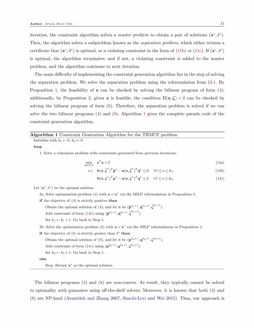
The main difficulty of implementing the constraint generation algorithm lies in the step of solving
the separation problem. We solve the separation problem using the reformulation from §3.1. By
Proposition 1, the feasibility of x can be checked by solving the bilinear program of form (4);
additionally, by Proposition 2, given x is feasible, the condition Π(x,ζ) < δ can be checked by
solving the bilinear program of form (8). Therefore, the separation problem is solved if we can
solve the two bilinear programs (4) and (8). Algorithm 1 gives the complete pseudo code of the
constraint generation algorithm.
Algorithm 1 Constraint Generation Algorithm for the TRMCF problem.Initialize with k1← 0, k2← 0.
loop
1. Solve a relaxation problem with constraints generated from previous iterations:
minx∈X ,δ
cTx+ δ (14a)
s.t. b(x, ζκ)T pκ−u(x, ζ
κ)T qκ ≤ 0, ∀1≤ κ≤ k1, (14b)
b(x,ζκ)Tpκ−u(x,ζκ)Tqκ ≤ δ, ∀1≤ κ≤ k2, (14c)
Let (x∗, δ∗) be the optimal solution.
2a. Solve optimization problem (4) with x = x∗ via the MILP reformulation in Proposition 3.
if the objective of (4) is strictly positive then
Obtain the optimal solution of (4), and let it be (pk1+1, qk1+1, ζk1+1
).
Add constraint of form (14b) using (pk1+1, qk1+1, ζk1+1
).
Set k1← k1 + 1. Go back to Step 1.
2b. Solve the optimization problem (8) with x = x∗ via the MILP reformulation in Proposition 4.
if the objective of (8) is strictly greater than δ∗ then
Obtain the optimal solution of (8), and let it be (pk2+1,qk2+1,ζk2+1).
Add constraint of form (14c) using (pk2+1,qk2+1,ζk2+1).
Set k2← k2 + 1. Go back to Step 1.
else
Stop. Return x∗ as the optimal solution.
The bilinear programs (4) and (8) are non-convex. As result, they typically cannot be solved
to optimality with guarantee using off-the-shelf solvers. Moreover, it is known that both (4) and
(8) are NP-hard (Atamturk and Zhang 2007, Simchi-Levi and Wei 2015). Thus, our approach is

Author: Article Short Title 12
to reformulate (4) and (8) to a pair of mixed integer linear programs (MILPs). While the MILP
formulation does not guarantee polynomial runtime, we observe through numerical experiment in
§4 that the MILP formulation usually can be solved efficiently using off-the-shelf MILP solvers.
For deriving MILP formulations, we use the following notations. Since b(x,ζ) and u(x,ζ) are
affine functions of x and ζ (Assumption 2), we write them explicitly as
b(x,ζ) =β(x) +Bζ, u(x,ζ) = υ(x) +Uζ,
where β(x) : X → Rn,υ(x) : X → Rm are affine mappings of x, and B ∈ Rn×`,U ∈ Rm×`
are fixed matrices. Since the uncertainty set U (a polytope) is bounded, we can find vectors
bmin,bmax,umin,umax such that
bmin ≤Bζ ≤ bmax, umin ≤Uζ ≤ umax, ∀ζ ∈ U .
Now, we derive an MILP reformulation for the bilinear program in the form of (4) by applying
the classical McCormick envelopes (McCormick 1976).
Proposition 3. The optimization problem (4) can be reformulated as
max 1Tz+β(x)Tp−1Tw−υ(x)Tq (15)
s.t. z≤ bmax ◦p, z≤Bζ−bmin ◦ (1−p)
w≥ umin ◦q, w≥Uζ−umax ◦ (1−q)
NTp≤ q
p∈ {0,1}n,q∈ {0,1}m,ζ ∈ U .
Proof. The first two sets of constraints in (15) are known as overestimates of z and underes-
timates of w in McCormick envelops. It is easily verified that z≤ (Bζ) ◦p and w≥ (Uζ) ◦ q are
implied by the first two constraints (recall that we use symbol “◦” to denote entry-wise product);
moreover, the inequality signs hold as equality in the optimal solution since the coefficients of z
and w in the objective function are positive and negative, respectively. Therefore, the objective
function of (15) is equal to
1Tz+β(x)Tp−1Tw−υ(x)Tq
=1T [(Bζ) ◦p] +β(x)Tp−1T [(Uζ) ◦q]−υ(x)Tq
=(Bζ)Tp+β(x)Tp− (Uζ)Tq−υ(x)Tq
=b(x,ζ)Tp−u(x,ζ)Tq,
and the last line is the objective function of optimization problem (4). �

Author: Article Short Title 13
We next develop an MILP reformulation for (8). Unlike formulation (4), the integer variables in
(8) are not binary, so we cannot directly apply the McCormick envelops to linearize the bilinear
terms in the objective function. To resolve this issue, we consider a reformulation of (8) where
the integer variables p, q, are replaced with their binary representations (Gupte et al. 2013). To
derive the binary representation, we use the fact that p is upper-bounded by pmax; and because
the objective of (8) for fixed p is maximized if we pick q= (NTp− f)+, if we let qmaxij = pmax
i − fij,
then q can be upper-bounded by qmax without loss of optimality. Therefore, we can replace pi and
qij by a set of binary variables pki and q`ij such that
pi =P∑k=0
2kpki , qij =
Q∑`=0
2`q`ij,
where P = maxi∈N{dlog2(pmaxi +1)e−1} and Q= max(i,j)∈A{dlog2(q
maxij +1)e−1}. With the binary
representations, we apply the McCormick envelops to reformulate (8).
Proposition 4. The optimization problem (8) can be formulated as
δ(x) = maxP∑k=0
2k(1Tzk +β(x)Tpk
)−
Q∑`=0
2`(1Tw`−υ(x)Tq`
)(16)
s.t. zk ≤ bmax ◦pk, zk ≤Bζ−bmin ◦ (1−pk), ∀k
w` ≥ umin ◦q`, w` ≥Uζ−umax ◦ (1−q`), ∀`
NT
(P∑k=0
2kpk
)−
Q∑`=0
2`q` ≤ f
∀k : pk ∈ {0,1}n,∀` : q` ∈ {0,1}m,ζ ∈ U .
Proof. The first two sets of constraints in (16) (McCormick envelops) ensure zk ≤ (Bζ)◦pk and
w` ≥ (Uζ)◦q`. Because the coefficients for zk are positive and the coefficients for w` are negative in
the objective function, if zk and wl are optimal, then zk = (Bζ)◦pk and w` = (Uζ)◦q`. Therefore,
letting p=∑P
k=0 2kpk, q=∑Q
`=0 2`q`, the objective of (16) is equal to
P∑k=0
2k(1Tzk +β(x)Tpk
)−
Q∑`=0
2`(1Tw`−υ(x)Tq`
)=
P∑k=0
2k(1T[(Bζ) ◦pk
]+β(x)Tpk
)−
Q∑`=0
2`(1T[(Uζ) ◦q`
]−υ(x)Tq`
)=
P∑k=0
2kb(x,ζ)Tpk−Q∑`=0
2`u(x,ζ)Tq`
=b(x,ζ)Tp−u(x,ζ)Tq,
and the last line is the objective of (8). The third constraint of (16) holds if and only if NTp−Iq≤ f .
So problem (16) is equivalent to the problem (8). �

Author: Article Short Title 14
It is important to note that when (pκ,qκ, ζκ) is an optimal solution for (4) or (8), the constraint
generated by (pκ,qκ, ζκ) in Algorithm 1 corresponds to exactly one constraint defined by Equation
(11b) or (11c), respectively. As a result, it is guaranteed that Algorithm 1 terminates in at most T
iterations, where T is the number of linear constraints in the reformulation (11). Recall from §3.1
that T is upper-bounded by (K + 1)n + 2n, where K only depends on the structure of the second
stage problem. Interestingly, this is in contrast to the standard constraint generation or cutting
plane algorithms proposed for general two-stage robust optimization problems (Thiele et al. 2010,
Zeng and Zhao 2013), where the number of constraints generated typically depends on the structure
of uncertainty sets. This observation is mainly of theoretical interest, as numerical examples suggest
that the actual number of constraints generated is typically much smaller than T .
A few comments are in order for implementing Algorithm 1. First, there are several advantages
of using the MILP reformulations instead of using the bilinear program formulations stated in
Algorithm 1 directly. Over the past few decades, there has been vast improvement in MILP solution
techniques, so solving (15) and (16) allows us to take advantage of the progress made in the
state-of-the-art MILP solvers. Moreover, at each iteration, we can use the MILP solution from the
previous iteration for warm start, therefore significantly reducing the computational time required
by MILP solvers. In our computational experiment, we use the Gurobi Mixed Integer Solver (7.0.2)
on a standard laptop, which is able to solve the separation problem for networks with hundreds of
nodes consistently in a few seconds.
Second, notice that in order to generate a constraint in Step 2a (or 2b) of Algorithm 1, it is
not necessary to solve the optimization problem to optimality. Instead, the algorithm can add a
cut whenever the MILP solver finds a feasible solution (p,q,ζ) such that the objective function is
strictly larger than zero (or δ). Using the solution (p,q,ζ), we can generate a valid constraint in
each iteration, while saving computation time by stopping the MILP solver early. After a feasible
solution (p,q,ζ) is found by the MILP solver, we can use it as an initial point to solve the bilinear
program form of the separation problem to local optimal using an alternating iterative method.
Namely, we fix either (p,q) or ζ while optimizing over the other, in order to strengthen the
constraint generated. Because the alternating iterative method only involves linear optimization,
it can be performed very fast. In our implementation of this method, the last iteration is always an
optimization over ζ with fixed (p,q), so it ensures that Algorithm 1 always generate a constraint
of form (11b) or (11c) in each iteration.
Third, when the uncertainty set lies in a unit hypercube, i.e., U ⊂ [0,1]r, there is an alternative
MILP reformulation of the separation problem. This reformulation is sometimes stronger than the
reformulations in Propositions 3 and 4, and is provably stronger for box uncertainty set, i.e., U =
[0,1]r. To define this formulation, we introduce continuous decision variables Z∈Rn×r,W ∈Rm×r.

Author: Article Short Title 15
Let 1n ∈ Rn,1m ∈ Rm, and 1r ∈ Rr be vectors with all elements equal to 1. Below is an MILP
reformulation for the optimization problem in Proposition 3. (The problem in Proposition 4 can
be reformulated using the same approach and is omitted here.)
Proposition 5. If U ⊂ [0,1]r, the optimization problem (4) can be reformulated as
max tr(BTZ) +β(x)Tp− tr(UTW)−υ(x)Tq (17)
s.t. Z≤ p1Tr , Z≤ 1nζT , Z≥ (1n−p)1Tr −1nζ
T , Z≥ 0
W≤ q1Tr , W≤ 1mζT , W≥ (1m−q)1Tr −1mζ
T , W≥ 0
NTp≤ q
p∈ {0,1}n,q∈ {0,1}m,ζ ∈ U .
Moreover, when U = [0,1]r, the optimal value of the LP relaxation of (17) is no greater than that
of the LP relaxation of (15).
Proof. In (17), since p and q are binary variables and 0 ≤ ζ ≤ 1, applying the McCormick
envelopes (McCormick 1976), the first two sets of constraints are equivalent to Z= pζT ,W = qζT .
Therefore, the objective function of (17) is equal to
tr(BTZ) +β(x∗)Tp− tr(UTW)−υ(x∗)Tq
=tr(BTpζT ) +β(x)Tp− tr(UTqζT )−υ(x)Tq
=ζTBTp+β(x)Tp− ζTUTq−υ(x)Tq
=b(x,ζ)Tp−u(x,ζ)Tq,
which is exactly the objective function of (4).
To prove the second part of the proposition, given a feasible solution to the LP relaxation of
(17), define z := diag(BZT ), w := diag(UWT ) (diag(·) here is the vector containing the diagonal
elements of a matrix). Let B+ =B∨0 and B− = (−B)∨0. Since Z≤ p1Tr , Z≥ 0, we have
z= diag(B+ZT )−diag(B−ZT )≤ diag(B+ ·1rpT )−0= diag(B+ ·1rpT ) = bmax ◦p,
where the last step follows from bmax := maxζ∈[0,1]r Bζ =B+1r. Since Z≤ 1nζT , Z≥ (1n−p)1Tr −
1nζT , we have
z=diag(B+ZT )−diag(B−ZT )≤ diag(B+ · ζ1Tn )−diag(B− · ζ1Tn )−diag(B− ·1r(1n−p)T )
= diag(B · ζ1Tn )−diag(B− ·1r(1n−p)T ) =Bζ−bmin ◦ (1−p),
where the last step follows from bmin := minζ∈[0,1]r Bζ = −B−1r. Similarly, one can prove that
w≥ umin ◦q, w≥Uζ−umax ◦ (1−q). Therefore, (z, w) is feasible for the LP relaxation of problem
(15). Finally, tr(BTZ) = tr(BZT ) = 1T z, tr(UTW) = tr(UWT ) = 1T w, so the optimal value of the
LP relaxation of (17) is no greater than that of the LP relaxation of (15). �
Author: Article Short Title 16
3.3. Column-and-Constraint Generation Algorithm
The efficiency of Algorithm 1 critically depends on the number of constraints generated until the
algorithm terminates. An approach commonly used in the two-stage robust optimization literature
to reduce the number of constraint generation iterations is the column-and-constraint generation
procedure introduced by Zeng and Zhao (2013). In this section, we present another algorithm for
the TRMCF problem. This second algorithm incorporates the MILP reformulations developed in
§3.2 into the column-and-constraint generation procedure of Zeng and Zhao (2013).
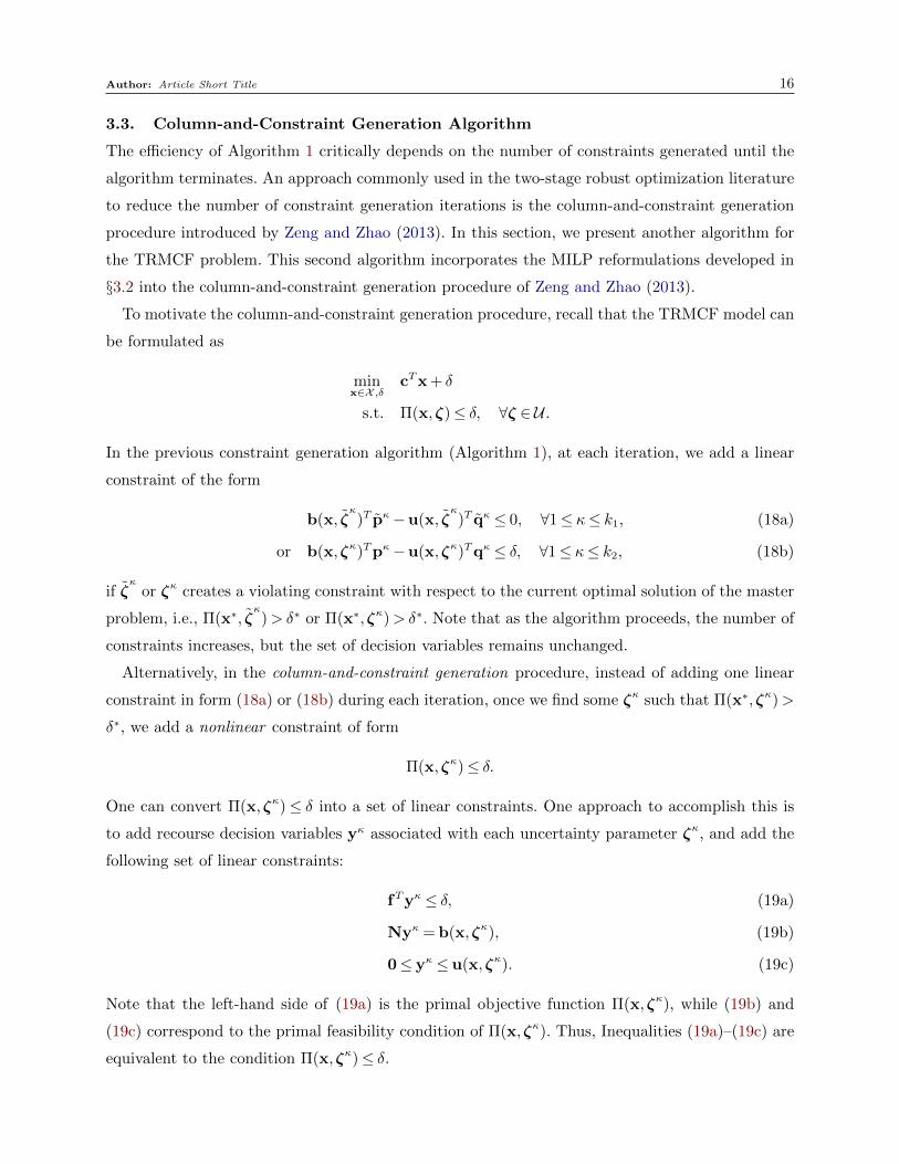
To motivate the column-and-constraint generation procedure, recall that the TRMCF model can
be formulated as
minx∈X ,δ
cTx+ δ
s.t. Π(x,ζ)≤ δ, ∀ζ ∈ U .
In the previous constraint generation algorithm (Algorithm 1), at each iteration, we add a linear
constraint of the form
b(x, ζκ)T pκ−u(x, ζ
κ)T qκ ≤ 0, ∀1≤ κ≤ k1, (18a)
or b(x,ζκ)Tpκ−u(x,ζκ)Tqκ ≤ δ, ∀1≤ κ≤ k2, (18b)
if ζκ
or ζκ creates a violating constraint with respect to the current optimal solution of the master
problem, i.e., Π(x∗, ζκ)> δ∗ or Π(x∗,ζκ)> δ∗. Note that as the algorithm proceeds, the number of
constraints increases, but the set of decision variables remains unchanged.
Alternatively, in the column-and-constraint generation procedure, instead of adding one linear
constraint in form (18a) or (18b) during each iteration, once we find some ζκ such that Π(x∗,ζκ)>
δ∗, we add a nonlinear constraint of form
Π(x,ζκ)≤ δ.
One can convert Π(x,ζκ)≤ δ into a set of linear constraints. One approach to accomplish this is
to add recourse decision variables yκ associated with each uncertainty parameter ζκ, and add the
following set of linear constraints:
fTyκ ≤ δ, (19a)
Nyκ = b(x,ζκ), (19b)
0≤ yκ ≤ u(x,ζκ). (19c)
Note that the left-hand side of (19a) is the primal objective function Π(x,ζκ), while (19b) and
(19c) correspond to the primal feasibility condition of Π(x,ζκ). Thus, Inequalities (19a)–(19c) are
equivalent to the condition Π(x,ζκ)≤ δ.

Author: Article Short Title 17
The separation problem for the column-and-constraint generation procedure requires checking
whether the optimization problem maxζ∈U Π(x∗,ζκ) has an optimal value greater than δ∗. Note
that this separation problem is the same separation problem solved in Algorithm 1. Therefore, as
in §3.2, we can convert maxζ∈U Π(x∗,ζκ) into two bilinear programs. Moreover, Propositions 3 and
4 show that the two bilinear programs can be reformulated as MILPs and solved using state-of-
the-art MILP solvers. Having described the intuition behind the column-and-constraint generation
procedure for the TRMCF problem, we formally define it in Algorithm 2.
We note that Zeng and Zhao (2013) have proposed an MILP formulation for solving the sepa-
ration problem of general two-stage robust linear programs with the additional relatively complete
recourse assumption. Ayoub and Poss (2016) extended the approach in Zeng and Zhao (2013) to
relax the relatively complete recourse assumption. Both Zeng and Zhao (2013) and Ayoub and Poss
(2016) uses the KKT conditions and their method can be applied if the second-stage problem is a
general LP. In contrast, our MILP reformulation of the separation problem exploits the network
flow structure of the second-stage problem, and thus is more compact (with fewer variables and
constraints) compared to methods in Zeng and Zhao (2013) and Ayoub and Poss (2016) for solving
the separation problem.
Algorithm 2 Column-and-Constraint Generation Algorithm for the TRMCF problem.Initialize with k← 0.
loop
1. Solve a relaxation of the TRMCF problem with k scenarios:
minx∈X ,y,δ
cTx+ δ (20)
s.t. fTyκ ≤ δ, ∀κ= 1, . . . , k
Nyκ = b(x,ζκ), ∀κ= 1, . . . , k
0≤ yκ ≤ u(x,ζκ), ∀κ= 1, . . . , k.
Let (x∗, δ∗) be the optimal solution.
2a. Solve optimization problem (4) with x = x∗ via the MILP reformulation in Proposition 3.
if the objective of (4) is strictly positive then
Let ζk+1 be the value of ζ in the optimal solution of (4). Go to Step 3.
2b. Solve the optimization problem (8) with x = x∗ via the MILP reformulation in Proposition 4.
if the objective of (8) is strictly greater than δ∗ then
Let ζk+1 be the value of ζ in the optimal solution of (8). Go to Step 3.
else
Stop. Return x∗ as an optimal solution.
3. Store ζk+1; create decision variables yk+1 ∈Rm, and add constraints (19a)–(19c) using ζk+1 and yk+1. Set
k← k+ 1. Go to Step 1.

Author: Article Short Title 18
In Algorithm 2, formulation (20) is equivalent to
minx∈X ,δ
cTx+ δ (21)
s.t. Π(x,ζκ)≤ δ,∀1≤ κ≤ k.
Thus, formulation (20) is a relaxation of the original TRMCF problem by partially enumerating a
small subset of scenarios in the uncertainty set U . Compared to formulation (14) from Algorithm 1
— which is another relaxation of the TRMCF problem — the relaxation (20) includes both x and
y variables, while (14) has only first-stage variables and fewer constraints. Moreover, the number
of y variables in (20) increases as the number of iterations k goes up. Therefore, with the same
number of iterations, Step 1 of Algorithm 2 usually requires more computation time than Step 1
of Algorithm 1. However, the benefit of introducing y variables in (2) is that at each iteration, it
generates much tighter constraints (i.e., cuts) to the relaxation of the TRMCF problem. In other
words, suppose (x∗, δ∗) is part of the optimal solution we obtained from Step 1 of Algorithm 2 and
there exists ζ∗ ∈ U such that Π(x∗,ζ∗)> δ∗. Then, the constraints generated by Algorithm 2 using
ζ∗ are stronger than the constraint generated by Algorithm 1 (Step 2a or Step 2b) using the same
ζ∗. This observation is formalized in the next proposition.
Proposition 6. Given any ζ∗ ∈ U , for any x∈X and δ, the condition Π(x,ζ∗)≤ δ implies the
following:
b(x,ζ∗)T p−u(x,ζ∗)T q≤ 0, for all (p, q) feasible for (4), (22a)
b(x,ζ∗)Tp−u(x,ζ∗)Tq≤ δ, for all (p,q) feasible for (8). (22b)
Proof. If x and δ satisfies Π(x,ζ∗) ≤ δ, then we obviously have Π(x,ζ∗) <∞, which by the
strong duality of the feasible flow problem (see Equation (3)), implies that (x, δ) satisfies Inequal-
ities (22a). Also, by taking the dual of the network problem representing Π(x,ζ∗) (see Equation
(7)), we have that Π(x,ζ∗)≤ δ implies (x, δ) satisfies Inequalities (22b). �.
By Proposition 6, each iteration of the column-and-constraint procedure is effectively adding
exponentially many constraints in the form of (22a)–(22b); in contrast, the constraint generation
procedure in §3.2 adds only a single constraint at each iteration that maximizes the left-hand-side
of (22a) and (22b). Therefore, the column-and-constraint generation algorithm usually terminate
in much fewer iterations than the constraint generation algorithm.
In §3.2, we argued that Algorithm 1 terminates within T steps, where T is the number of linear
constraints in the reformulation given by Theorem 1. It turns out that Algorithm 2 has a slightly
stronger theoretical termination guarantee: the maximum number of iterations is bounded by the
number of extreme points of the uncertainty set, or T , whichever is smaller.

Author: Article Short Title 19
Corollary 2. The number of iterations of Algorithm 2 is bounded by
min{|ext(U)|, T},
where ext(U) is the set of extreme points of uncertainty set U , and T is the number of linear
constraints in formulation (11) from Theorem 1.
Proof. Let k denote the number of iterations of Algorithm 2. First, we show that k≤ |ext(U)|.For each iteration κ= 1, . . . , k, scenario ζκ is either an optimal solution of (4) or (8). In both cases,
ζκ is an extreme point of U . By Step 1 of Algorithm 2, the same ζκ cannot be generated more
than once. Therefore, we have k≤ |ext(U)|.Next, we show that k ≤ T . For each iteration κ= 1, . . . , k, if scenario ζκ is generated from Step
2a, then by Proposition 6, Π(x,ζκ)≤ δ includes at least one constraint of form (11b); and if the
scenario ζκ is generated from Step 2b, Π(x,ζκ)≤ δ includes at least one constraint of form (11c).
Because the same constraint cannot be generated more than once, we have k ≤ T , the number of
constraints of form (11b) or (11c). This complete the proof. �
To see the bound from Corollary 2 is indeed an improvement over either |ext(U)| or T , consider
U1 = {ζ ∈Rn :n∑i=1
(ζi− k)+ ≤ (n− k+ 1)(n− k)
2, ∀1≤ k≤ n},
and U2 = {ζ ∈Rn :n∑i=1
ζi = (n− 1)l+u, l≤ ζi ≤ u,∀1≤ i≤ n}.
First, observe that ζ∗ = [1,2, . . . , n]T is an extreme point in U1. Because U1 is defined symmetrically,
if we permute the entries in ζ∗ by any permutation, we get a different extreme point in U1, as
the entires in ζ∗ are unique. Therefore, U1 has at least n! extreme points, and since T grows
exponentially with a constant base, we have |ext(U1)|> T when n is large enough. Next, observe
that ext(U2) is consisted of all vectors with n − 1 entries equal to u and one entry equal to l.
Therefore, we have that |ext(U2)| = n and hence |ext(U2)| < T for large n. Finally, we note that
Corollary 2 is mainly of theoretical interest. In numerical studies, we observe that Algorithm 2
typically converges in several iterations, much smaller than the value of min{|ext(U)|, T}.We conclude §3.3 by stating that in our numerical examples, the column-and-constraint gener-
ation (C&CG) algorithm usually converges faster than the constraint generation (CG) algorithm,
confirming the intuition behind Proposition 6 and Corollary 2. However, the C&CG algorithm does
significantly increase the complexity of the master problem (the optimization problem solved in
Step 1 of Algorithm 1 and 2). While our numerical results consistently show that C&CG is the
superior method, when the master problem is difficult to solve, it is possible that C&CG algorithm
spends much longer time each iteration and therefore result in an inferior performance compared
to the CG algorithm.

Author: Article Short Title 20
4. Numerical Examples and Applications
In this section, we test the constraint generation (CG) algorithm and the column-and-constraint
generation (C&CG) algorithm using numerical examples.
4.1. Joint Inventory-Transportation Problem
We consider a classical problem in logistics with joint inventory and transportation decisions. The
problem can be naturally formulated into the two-stage robust optimization framework, and several
variants of this problem have been studied in the robust optimization literature by Atamturk and
Zhang (2007), Gabrel et al. (2014a), Ardestani-Jaafari and Delage (2017), Bertsimas and de Ruiter
(2016).
Suppose a firm needs to distribute a product through a network with multiple supply nodes
(i= 1, . . . ,Ns) and multiple demand nodes (j = 1, . . . ,Nd). In the first stage, the firm determines the
storage level (xi) at each supply node, without actual demand realization. We assume the demand
realization at all demand nodes is given by d(ζ) = d+σ ◦ζ, where ζ belongs to an uncertainty set
of the following form:
U = {ζ ∈RNd :−1≤ ζ ≤ 1, |ζ|1 ≤ β,1Tζ ≤ γ}.
Here, σ limits demand variation of each individual demand node, while parameters β and γ bound
the aggregate demand variation across all the demand nodes. We note that U is not a budget
uncertainty set in the form of Bertsimas and Sim (2004). In the special case with γ = +∞, U
becomes a budget uncertainty set. Furthermore, when β is an integer, U is a 0-1 polytope. In that
case, it is known that the separation problem can be solved by enumerating all extreme points of
U or by applying the MILP reformulation (see Thiele et al. 2010, Zeng and Zhao 2013, Ayoub and
Poss 2016). However, in the general case with γ <+∞, the set U does not admit a compact 0-1
polytope representation. In the algorithms we use below, we treat U as a general polyhedral set.
We assume that inventory stored at supply node i in the first stage incurs a unit holding cost of
ci. In the second stage, parameter ζ (and demand d(ζ)) is realized, and the firm must transport
items from the supply nodes to the demand nodes through a bipartite network with arcs A. A flow
from supply node i to demand node j has a unit transportation cost of fij. The problem can be
formulated as follows:
minx≥0
maxζ∈U
miny≥0
Ns∑i=1
cixi +∑
(i,j)∈A
fijyij (23)
s.t.∑
j:(i,j)∈A
yij ≤ xi, ∀i= 1, . . . ,Ns∑i:(i,j)∈A
yij = dj(ζ), ∀j = 1, . . . ,Nd.
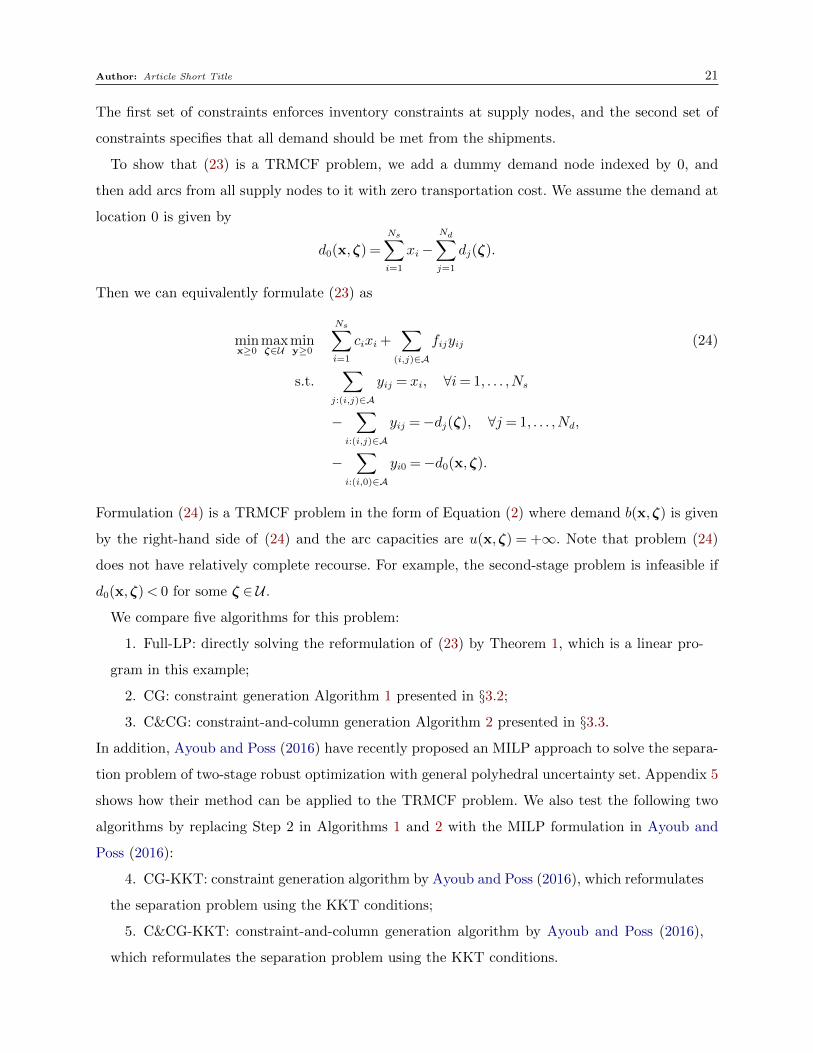
Author: Article Short Title 21
The first set of constraints enforces inventory constraints at supply nodes, and the second set of
constraints specifies that all demand should be met from the shipments.
To show that (23) is a TRMCF problem, we add a dummy demand node indexed by 0, and
then add arcs from all supply nodes to it with zero transportation cost. We assume the demand at
location 0 is given by
d0(x,ζ) =
Ns∑i=1
xi−Nd∑j=1
dj(ζ).
Then we can equivalently formulate (23) as
minx≥0
maxζ∈U
miny≥0
Ns∑i=1
cixi +∑
(i,j)∈A
fijyij (24)
s.t.∑
j:(i,j)∈A
yij = xi, ∀i= 1, . . . ,Ns
−∑
i:(i,j)∈A
yij =−dj(ζ), ∀j = 1, . . . ,Nd,
−∑
i:(i,0)∈A
yi0 =−d0(x,ζ).
Formulation (24) is a TRMCF problem in the form of Equation (2) where demand b(x,ζ) is given
by the right-hand side of (24) and the arc capacities are u(x,ζ) = +∞. Note that problem (24)
does not have relatively complete recourse. For example, the second-stage problem is infeasible if
d0(x,ζ)< 0 for some ζ ∈ U .
We compare five algorithms for this problem:
1. Full-LP: directly solving the reformulation of (23) by Theorem 1, which is a linear pro-
gram in this example;
2. CG: constraint generation Algorithm 1 presented in §3.2;
3. C&CG: constraint-and-column generation Algorithm 2 presented in §3.3.
In addition, Ayoub and Poss (2016) have recently proposed an MILP approach to solve the separa-
tion problem of two-stage robust optimization with general polyhedral uncertainty set. Appendix 5
shows how their method can be applied to the TRMCF problem. We also test the following two
algorithms by replacing Step 2 in Algorithms 1 and 2 with the MILP formulation in Ayoub and
Poss (2016):
4. CG-KKT: constraint generation algorithm by Ayoub and Poss (2016), which reformulates
the separation problem using the KKT conditions;
5. C&CG-KKT: constraint-and-column generation algorithm by Ayoub and Poss (2016),
which reformulates the separation problem using the KKT conditions.

Author: Article Short Title 22
We first test a setting without second-stage transportation costs. We generate four groups of
bipartite networks with numbers of nodes ranging from 20 to 500. Each group includes 100 random
problem instances. We assume the number of warehouses and number of demand locations are
equal, and each demand location can be served by a random number of warehouses which is
uniformly distributed between 1 and 10. The inventory holding cost at each warehouse is uniformly
distributed between 1 and 10.
The tests were performed using the Gurobi 7.0.2 solver on a 2.8GHz Intel CPU. In Table 1,
we show the average CPU time of different algorithms. By Corollary 1, the linear programming
reformulation of this special case has exactly 2n constraints, where n is the number of nodes in the
network. In this example, because the network is bipartite and there is no uncertainty associated
with supply nodes (warehouses), we can further reduce the number of constraints to 2Nd = 2n/2.
We notice that for networks with small size (n= 20), the speed of Full-LP is comparable to CG and
C&CG. However, when the network size grows, Full-LP quickly becomes impractical to solve since
the number of constraints grows exponentially fast. Full-LP is not able to solve for networks with
more than 100 nodes. CG is able to solve network with hundreds of nodes. C&CG is extremely
efficient, and is able to solve a logistics network with 500 nodes under 3 seconds. The CG and
C&CG algorithms by Ayoub and Poss (2016) (CG-KKT and C&CG-KKT), on the other hand,
require significantly longer CPU time than our CG and C&CG algorithms and even the Full-LP
algorithm. When the number of nodes is greater than 50, the method by Ayoub and Poss (2016)
does not terminate in six hours for a single test instance, so we are not able to report average
CPU time for n≥ 50. When n= 20, the method by Ayoub and Poss (2016) is about 10,000 times
slower than our CG and C&CG algorithms. We note that while our algorithms exploit the network
flow structure of the second-stage problem, the method of Ayoub and Poss (2016) assumes the
second-stage problem is a general LP. In spite of its generality, Ayoub and Poss (2016) mentioned
that their method might be inefficient because it involves a large number of binary variables and
uses big-M reformulation.
Table 1 also lists a few additional statistics about the various algorithms we tested. “Number
of iterations” gives the average number of iterations in CG, C&CG, CG-KKT, and C&CG-KKT
before the optimal solution is found. “MIP/LP ratio” measures the average ratio of the optimal
value of an MILP reformulation of the separation problem and its LP relaxation; since the value of
the MILP is positive (otherwise the algorithm terminates), the ratio is between 0 and 1, and a ratio
close to 1 means the LP relaxation is tight. “% of time on SP” shows the percentage of the time
that CG and C&CG algorithms spend on solving separation problems, i.e., step 2 in Algorithms 1
and 2.
Author: Article Short Title 23
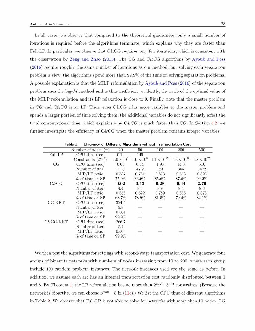
In all cases, we observe that compared to the theoretical guarantees, only a small number of
iterations is required before the algorithms terminate, which explains why they are faster than
Full-LP. In particular, we observe that C&CG requires very few iterations, which is consistent with
the observation by Zeng and Zhao (2013). The CG and C&CG algorithms by Ayoub and Poss
(2016) require roughly the same number of iterations as our method, but solving each separation
problem is slow: the algorithms spend more than 99.9% of the time on solving separation problems.
A possible explanation is that the MILP reformulation by Ayoub and Poss (2016) of the separation
problem uses the big-M method and is thus inefficient; evidently, the ratio of the optimal value of
the MILP reformulation and its LP relaxation is close to 0. Finally, note that the master problem
in CG and C&CG is an LP. Thus, even C&CG adds more variables to the master problem and
spends a larger portion of time solving them, the additional variables do not significantly affect the
total computational time, which explains why C&CG is much faster than CG. In Section 4.2, we
further investigate the efficiency of C&CG when the master problem contains integer variables.
Table 1 Efficiency of Different Algorithms without Transportation Cost
Number of nodes (n) 20 50 100 200 500Full-LP CPU time (sec) 0.12 149 — — —
Constraints (2n/2) 1.0× 10³ 1.0× 10⁶ 1.1× 10¹⁵ 1.3× 1030 1.8× 1075
CG CPU time (sec) 0.03 0.34 1.98 14.0 516Number of iter. 11.3 47.2 123 365 1472MIP/LP ratio 0.837 0.781 0.853 0.853 0.823
% of time on SP 75.0% 83.9% 85.6% 87.6% 90.2%C&CG CPU time (sec) 0.02 0.13 0.28 0.44 2.70
Number of iter. 4.4 8.5 8.9 8.4 8.3MIP/LP ratio 0.656 0.622 0.789 0.858 0.878
% of time on SP 68.7% 78.9% 81.5% 79.4% 84.1%CG-KKT CPU time (sec) 324.5 — — — —
Number of iter. 9.8 — — — —MIP/LP ratio 0.004 — — — —
% of time on SP 99.9% — — — —C&CG-KKT CPU time (sec) 266.7 — — — —
Number of Iter. 5.4 — — — —MIP/LP ratio 0.003 — — — —
% of time on SP 99.9% — — — —
We then test the algorithms for settings with second-stage transportation cost. We generate four
groups of bipartite networks with numbers of nodes increasing from 10 to 200, where each group
include 100 random problem instances. The network instances used are the same as before. In
addition, we assume each arc has an integral transportation cost randomly distributed between 1
and 8. By Theorem 1, the LP reformulation has no more than 2n/2 +8n/2 constraints. (Because the
network is bipartite, we can choose pmax = 8 in (11c).) We list the CPU time of different algorithms
in Table 2. We observe that Full-LP is not able to solve for networks with more than 10 nodes. CG

Author: Article Short Title 24
and C&CG are able to solve networks with 100 nodes, and again C&CG is much faster than CG
and terminates in much fewer iterations. Similar to the results in Table 1, the method of Ayoub
and Poss (2016) is slow and is not able to solve networks with more than 20 nodes. The MILP
reformulation of the separation problem has a nearly zero MIP/LP ratio, and the algorithms spend
more than 99.9% of the time on solving separation problems.
Table 2 Efficiency of Different Algorithms with Transportation Cost
Number of nodes (n) 10 20 50 100Full-LP CPU time (sec) 3.34 — — —
Total constraints 3.3× 10⁴ 1.1× 10⁹ 3.8× 10²² 1.4× 1045
CG CPU time (sec) 0.05 0.35 22.3 480Number of iter. 5.8 13.9 64.9 213MIP/LP ratio 0.763 0.590 0.437 0.438
% of time on SP 92.6% 97.5% 99.8% 99.9%C&CG CPU time (sec) 0.04 0.17 16.1 66.7
Number of iter. 2.8 4.6 12.2 25.5MIP/LP ratio 0.627 0.463 0.272 0.243
% of time on SP 90.6% 95.3% 98.9% 99.6%CG-KKT CPU time (sec) 1.02 321.3 — —
Number of iter. 7.4 16 — —MIP/LP ratio 0.001 0.000 — —
% of time on SP 98.8% 99.9% — —C&CG-KKT CPU time (sec) 0.95 224.8 — —
Number of iter. 3.2 7.5 — —MIP/LP ratio 0.000 0.000 — —
% of time on SP 98.6% 99.9% — —
4.2. Joint Location-Transportation Problem
In this example, we extend the previous lot-sizing and transportation setting by including facility
location decisions. For each supply node i= 1, . . . ,Ns, let zi ∈ {0,1} be a binary variable indicating
if a facility is open at location i. If the facility at location i is open, we assume a fixed cost gi is
incurred, and the facility has capacity Ki. The other model assumptions remain the same as in the
previous lot-sizing/ transportation example. Then, the two-stage robust location-transportation
problem is formulated as follows:
minx,z
maxζ
miny
Ns∑i=1
gizi +
Ns∑i=1
cixi +∑
(i,j)∈A
fijyij (25)
s.t. xi ≤Kizi, ∀i= 1, . . . ,Ns∑j:(i,j)∈A
yij ≤ xi, ∀i= 1, . . . ,Ns∑i:(i,j)∈A
yij = dj(ζ), ∀j = 1, . . . ,Nd
x≥ 0, z∈ {0,1}Ns , ζ ∈ U , y≥ 0.

Author: Article Short Title 25
Similar to §4.1, we test CG (Algorithm 1), C&CG (Algorithm 2), CG-KKT and C&CG-KKT
for this problem. We randomly generate four groups of networks with numbers of nodes ranging
from 10 to 100. We use the same demand uncertainty sets and cost parameters defined in §4.1. We
assume that the fixed cost is gi = 5 and capacity is Ki = 10.
Table 3 lists the CPU time, number of iterations, MIP/LP ratio, and percentage of time spent
on separation problems for different algorithms (see the definition of these statistics in §4.1).
Compared with Table 2, we find that adding first-stage binary variables does not significantly affect
the computation time of CG and C&CG when n≤ 50. This is because even if the master problem
is now an MILP, the number of iterations (and thus the size of the master problem) is small when
n≤ 50. When n= 100, the computation time of CG becomes significantly worse. The reason is that
CG needs to add about 500 constraints to the master problem. The master problem, now having
binary variables, becomes harder and harder to solve as more constraints are added.
Surprisingly, the C&CG algorithm remains efficient for n= 100, even if the algorithm adds more
constraints and variables to the master problem per iteration. We suspect that the reason is that
C&CG terminates after only 22 iterations, while CG terminates after 581 iterations on average.
Therefore, the size of the master problem of C&CG is still smaller than that of CG, even if it adds
more variables and constraints per iteration. Finally, similar to §4.1, CG-KKT and C&CG-KKT
cannot solve networks with more than 20 nodes.
Table 3 Efficiency of Different Algorithms with Location Decisions
Number of nodes (n) 10 20 50 100Total constraints 3.3× 10⁴ 1.1× 10⁹ 3.8× 10²² 1.4× 1045
CG CPU time (sec) 0.07 0.46 32.8 4849Number of Iter. 5.4 13.9 91.8 581MIP/LP ratio 0.834 0.696 0.578 0.579
% of time on SP 77.1% 80.6% 61.2% 8.6%C&CG CPU time (sec) 0.05 0.22 7.8 71.7
Number of Iter. 2.6 3.9 11.3 21.9MIP/LP ratio 0.687 0.513 0.313 0.307
% of time on SP 78.0% 78.4% 66.7% 50.8%CG-KKT CPU time (sec) 4.19 — — —
Number of Iter. 6.1 — — —MIP/LP ratio 0.004 — — —
% of time on SP 98.4% — — —C&CG-KKT CPU time (sec) 1.74 — — —
Number of Iter. 2.4 — — —MIP/LP ratio 0.005 — — —
% of time on SP 98.7% — — —
4.3. Production Postponement
We next perform numerical experiment on a production postponement application described in
Chou et al. (2014), which is based on the Sports Obermeyer Ltd. case by Hammond and Raman

Author: Article Short Title 26
(1994). In this application, Sports Obermeyer Ltd. sells ten different styles of parkas. The company
is required to order a portion of its parkas before demand is realized, while the rest of the order
can be postponed after demand is revealed. Each style j has its own price, and its demand follows
normal distribution with mean µj and standard deviation σj that is truncated at zero. The price,
mean demand, and standard deviation of demand for different styles are listed in Table 4. Demand
is lost if there is not enough parkas produced, and lost sales cost of each parka style j is equal to
24% of its price.
Table 4 Sports Obermeyer Data
Demand and price information for different stylesGail Isis Entice Assault Tri Electra Stephanie Seduced Anita Daphane
ID (j) 1 2 3 4 5 6 7 8 9 10Mean (µj) 1017 1042 1358 2525 1100 2150 1113 4017 3296 2383Std.v. (σj) 194 323 248 340 381 404 524 556 1047 697Price (πj) 110 99 80 90 123 173 133 73 93 148
In the first stage, Sports Obermeyer Ltd. needs to produce a total of C units of parkas. In the
second stage, after the demand d(ζ) (defined as d(ζ) = µ + ζ ◦σ) is realized, the firm produces
the remaining parkas from its ten facilities. We use x and y to denote the first and second-stage
production quantities, respectively. For 1 ≤ i ≤ 10, facility i has (second-stage) capacity ci. The
production capability of facilities is represented by set F , where (i, j)∈F implies that facility i is
capable of producing style j. In sum, the decisions of Sports Obermeyer Ltd. can be modeled as
the following two-stage robust optimization problem:
minx≥0
maxζ∈U
miny,l≥0
10∑j=1
ujlj (26)
s.t.∑
i: (i,j)∈F
yij + lj ≥ dj(ζ)−xj, ∀1≤ j ≤ 10,∑j: (i,j)∈F
yij ≤ ci, ∀1≤ i≤ 10,
10∑j=1
xj =C.
The objective of (26) is to minimize worst-case lost sales, where uj is the lost sales cost. The first
set of constraints specifies that demand not met is lost. The second set of constraints specifies the
production capacity at the second stage. The third constraint represents the production capacity
at the first stage. We assume uncertainty set U to be all ζ satisfying
U = {ζ :10∑j=1
|ζj| ≤ Γ,−2≤ ζj ≤ 2,∀1≤ j ≤ 10}.

Author: Article Short Title 27
Recall that d(ζ) = µ + ζ ◦σ, thus, our choice of uncertainty set essentially uses Γ to bound the
aggregate demand variations, and ensures for each individual style, its demand does not deviate
more than two standard deviation away from its mean.
The second-stage minimization problem in (26) can be converted into a minimum cost flow
problem. Therefore, we can convert (26) into a TRMCF problem, and solve it using algorithms
developed in §3. Also, it is easy to check that any first-stage decision x ≥ 0 is feasible for (26),
implying that problem (26) has relatively complete recourse. As a result, by Corollary 1, the
reformulation of TRMCF for problem (26) is simpler than the general TRMCF model. Finally, we
can also take advantage of the specific structures in (26) to show that the dual of the second stage
network flow problem can be rewritten as an integer program with just integer variables {pj}10j=1,
and constraints pj ≤ uj for 1≤ j ≤ 10. This implies that the reformulation of TRMCF have at most
linear Π10j=1(uj + 1) constraints.
Like §4.1 and 4.2, we test the performance of the constraint generation (CG) algorithm and
the constraint-and-column generation (C&CG) algorithm for this postponement problem. We ran-
domly generate test instances as follows. We generate F by starting with the set {(i, i)|1≤ i≤ 10},
implying facility i can always produce parka style i. Then for any i, j with i 6= j, we add arc (i, j)
with probability 0.1. The additional arcs represent the flexibility of facilities for producing different
styles. The first-stage capacity parameter C is drawn uniformly at random from [0.7µT ,0.9µT ].
where µT =∑
1≤j≤10 µj. The second-stage capacity is assumed to be 20% of the expected demand
of style i, i.e., ci = 0.2µi. The parameter Γ is drawn uniformly at random from [2.5,6.5]. Finally,
because our algorithms require the coefficient of the objective function (uj) to be integers, we
rescale and round lost sales cost uj in increments of U by rounding uj to the nearest integer to
0.24 · πj/U for U ∈ {10,4,1,0.1}. Note that a bigger U implies that uj is smaller after rounding.
Therefore the total number of constraints in formulation (11) decreases as we increase the rounding
unit U , which improves our computational time. However, picking a big rounding unit U decreases
the precision of our estimation to the true lost sales cost.
In Table 5, we list the CPU time of different methods under different rounding unit. For the
Full-LP algorithm, we list the number of constraints in the LP formulation in the table; however,
as most of instances contains too many constraints, it is impractical to apply the Full-LP algorithm
for this problem. Like §4.1 and 4.2, we observe that C&CG is always faster than CG and requires
less iterations across different rounding units. Since problem (26) has relatively complete recourse,
we were also able to apply the method in Zeng and Zhao (2013) for solving two-stage robust
optimization with general polyhedral sets. The results are reported as CG-KKT and C&CG-KKT
in Table 5. Notice that the method in Zeng and Zhao (2013) does not require the second-stage cost
to be integral, so there is only one column of results. We observe that the method by Zeng and Zhao
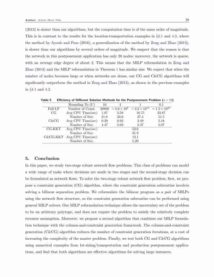
Author: Article Short Title 28
(2013) is slower than our algorithms, but the computation time is of the same order of magnitude.
This is in contrast to the results for the location-transportation examples in §4.1 and 4.2, where
the method by Ayoub and Poss (2016), a generalization of the method by Zeng and Zhao (2013),
is slower than our algorithms by several orders of magnitude. We suspect that the reason is that
the network in this postponement application has only 20 nodes; moreover, the network is sparse,
with an average edge degree of about 2. This means that the MILP reformulation in Zeng and
Zhao (2013) and the MILP reformulation in Theorem 1 has similar size. We expect that when the
number of nodes becomes large or when networks are dense, our CG and C&CG algorithms will
significantly outperform the method in Zeng and Zhao (2013), as shown in the previous examples
in §4.1 and 4.2.
Table 5 Efficiency of Different Solution Methods for the Postponement Problem (n= 10)
Rounding To (U) 10 4 1 0.1Full-LP Number of Const. 38800 ∼ 5.6× 10⁸ ∼ 2.2× 10¹⁴ ∼ 1.5× 1024
CG Avg CPU Time(sec) 1.07 3.59 16.75 33.87Number of Iter. 21.8 33.6 37.4 51.5
C&CG Avg CPU Time(sec) 0.29 0.92 3.49 5.18Number of Iter. 4.47 5.03 5.37 5.07
CG-KKT Avg CPU Time(sec) 53.6Number of Iter. 31.9
C&CG-KKT Avg CPU Time(sec) 13.1Number of Iter. 5.29
5. Conclusion
In this paper, we study two-stage robust network flow problems. This class of problems can model
a wide range of tasks where decisions are made in two stages and the second-stage decision can
be formulated as network flows. To solve the two-stage robust network flow problem, first, we pro-
pose a constraint generation (CG) algorithm, where the constraint generation subroutine involves
solving a bilinear separation problem. We reformulate the bilinear program as a pair of MILPs
using the network flow structure, so the constraint generation subroutine can be performed using
general MILP solvers. Our MILP reformulation technique allows the uncertainty set of the problem
to be an arbitrary polytope, and does not require the problem to satisfy the relatively complete
recourse assumption. Moreover, we propose a second algorithm that combines our MILP formula-
tion technique with the column-and-constraint generation framework. The column-and-constraint
generation (C&CG) algorithm reduces the number of constraint generation iterations, at a cost of
increasing the complexity of the master problem. Finally, we test both CG and C&CG algorithms
using numerical examples from lot-sizing/transportation and production postponement applica-
tions, and find that both algorithms are effective algorithms for solving large instances.

Author: Article Short Title 29
Appendix
A. An alternative MILP reformulation of the separation problem using KKTconditions
Ayoub and Poss (2016) proposed an MILP reformulation of the separation problem for two-stage robust
optimization. The reformulation applies to general second-stage problems under general polyhedral uncer-
tainty, without assuming relatively complete recourse. The key idea of Ayoub and Poss (2016) is to formulate
the separation problem as a bilevel optimization problem and then use big-M method to linearize comple-
mentary slackness conditions (referred to as KKT conditions in Zeng and Zhao (2013)). Similar ideas have
appeared in Mattia (2013), Zeng and Zhao (2013). We present the method by Ayoub and Poss (2016) below
in the context of robust network flow problems.
Let (x, δ) be a first-stage solution to the TRMCF problem (2). By definition, the solution is feasible if and
only if Π(x,ζ)≤ δ, ∀ζ ∈ U . Equivalently, by Eq (1), (x, δ) is feasible when the optimization problem below
has an optimal objective value equal to 0.
maxζ∈U
miny
0
s.t. fTy≤ δ
Ny = b(x,ζ)
0≤ y≤ u(x,ζ).
By strong duality, we can reformulate the problem above as
maxζ∈U
maxp,q
b(x,ζ)Tp−u(x,ζ)Tq− δr
s.t. NTp− Iq− rf ≤ 0
p∈Rn,q∈Rm+ , r≥ 0.
Because N is the node-arc incidence matrix and 1Tnb(x,ζ) = 0 by flow balance condition, we can assume
p≥ 0 without changing optimal value of the objective. Moreover, given any solution (p,q, r), we can rescale
all the decision variables by the same positive constant factor without changing the sign of the objective
function. Therefore, (x, δ) is feasible for the first-stage problem if and only if the optimization problem below
has a nonpositive optimal value (i.e., g(x, δ)≤ 0).
g(x, δ) = maxζ∈U
maxp,q
b(x,ζ)Tp−u(x,ζ)Tq− δr
s.t. NTp− Iq− rf ≤ 0 (27a)
pT1n +qT1m + r≤ 1 (27b)
p∈Rn+,q∈Rm+ , r≥ 0.
By strong duality again, we have
g(x, δ) = maxζ∈U
miny≥0,z≥0
z
s.t. − fTy+ z ≥−δ (28a)
Ny+ z1n ≥ b(x,ζ) (28b)
−y+ z1m ≥−u(x,ζ). (28c)

Author: Article Short Title 30
This is a bilevel optimization problem. Note that the lower-level problem always has a finite optimal value
since the feasible set (27a)–(27b) is bounded and nonempty (p = 0,q = 0, r = 0 is a feasible solution).
Therefore, we can rewrite the lower-level problem by KKT conditions as
g(x, δ) = maxζ,y,z,p,q,r
z (29a)
s.t. (27a)− (28c)
[Ny+ z1n−b(x,ζ)]Tp= 0 (29b)
[−y+ z1m +u(x,ζ)]Tq = 0 (29c)[
−fTy+ z+ δ]r= 0 (29d)[
NTp− Iq− rf]T
y = 0 (29e)[pT1n +qT1m + r− 1
]Tz = 0 (29f)
ζ ∈ U ,p∈Rn+,q∈Rm+ , r≥ 0,y ∈Rm+ , z ≥ 0.
Equations (27a)–(28c) guarantee primal and dual feasibility, and the constraints (29b)–(29f) guarantee the
KKT conditions. The KKT conditions are special ordered sets of type 1 (SOS-1). They can also be represented
as linear constraints using binary variables and big-M method. For example, if we introduce a vector of
binary variables µ for constraint (29b), then it can be reformulated as
Ny+ z1n−b(x,ζ)≤Mµ, p≤M(1n−µ), µ∈ {0,1}n.
The other constraints can be reformulated similarly. Therefore, the bilevel problem (29) can be solved as an
MILP, and the first-stage variables (x, δ) is feasible if and only if g(x, δ)≤ 0.
References
Agra, A., Christiansen, M., Figueiredo, R., Hvattum, L. M., Poss, M., and Requejo, C. (2013). The robust
vehicle routing problem with time windows. Computers & Operations Research, 40(3):856–866.
Ahuja, R. K., Magnanti, T. L., and Orlin, J. B. (1993). Network flows: theory, algorithms, and applications.
Prentice hall.
Ardestani-Jaafari, A. and Delage, E. (2016). Robust optimization of sums of piecewise linear functions with
application to inventory problems. Operations research, 64(2):474–494.
Ardestani-Jaafari, A. and Delage, E. (2017). The value of flexibility in robust location–transportation prob-
lems. Transportation Science.
Atamturk, A. and Zhang, M. (2007). Two-stage robust network flow and design under demand uncertainty.
Operations Research, 55(4):662–673.
Ayoub, J. and Poss, M. (2016). Decomposition for adjustable robust linear optimization subject to uncer-
tainty polytope. Computational Management Science, 13(2):219–239.
Ben-Tal, A., Do Chung, B., Mandala, S. R., and Yao, T. (2011). Robust optimization for emergency logis-
tics planning: Risk mitigation in humanitarian relief supply chains. Transportation Research Part B:
Methodological, 45(8):1177–1189.

Author: Article Short Title 31
Ben-Tal, A., El Ghaoui, L., and Nemirovski, A. (2009). Robust optimization. Princeton University Press.
Ben-Tal, A., Golany, B., Nemirovski, A., and Vial, J.-P. (2005). Retailer-supplier flexible commitments con-
tracts: A robust optimization approach. Manufacturing & Service Operations Management, 7(3):248–
271.
Ben-Tal, A., Goryashko, A., Guslitzer, E., and Nemirovski, A. (2004). Adjustable robust solutions of uncer-
tain linear programs. Mathematical Programming, 99(2):351–376.
Bertsimas, D. and Caramanis, C. (2010). Finite adaptability in multistage linear optimization. IEEE
Transactions on Automatic Control, 55(12):2751–2766.
Bertsimas, D. and de Ruiter, F. J. (2016). Duality in two-stage adaptive linear optimization: Faster compu-
tation and stronger bounds. INFORMS Journal on Computing, 28(3):500–511.
Bertsimas, D. and Goyal, V. (2012). On the power and limitations of affine policies in two-stage adaptive
optimization. Mathematical programming, 134(2):491–531.
Bertsimas, D., Iancu, D. A., and Parrilo, P. A. (2010). Optimality of affine policies in multistage robust
optimization. Mathematics of Operations Research, 35(2):363–394.
Bertsimas, D., Litvinov, E., Sun, X. A., Zhao, J., and Zheng, T. (2013a). Adaptive robust optimization for the
security constrained unit commitment problem. IEEE Transactions on Power Systems, 28(1):52–63.
Bertsimas, D., Nasrabadi, E., and Stiller, S. (2013b). Robust and adaptive network flows. Operations
Research, 61(5):1218–1242.
Bertsimas, D. and Sim, M. (2003). Robust discrete optimization and network flows. Mathematical Program-
ming, 98(1):49–71.
Bertsimas, D. and Sim, M. (2004). The price of robustness. Operations Research, 52(1):35–53.
Billionnet, A., Costa, M.-C., and Poirion, P.-L. (2014). 2-stage robust milp with continuous recourse variables.
Discrete Applied Mathematics, 170:21–32.
Birge, J. R. and Louveaux, F. (2011). Introduction to stochastic programming. Springer Science & Business
Media.
Bonami, P., Kilinc, M., and Linderoth, J. (2012). Algorithms and software for convex mixed integer nonlinear
programs. In Mixed Integer Nonlinear Programming, pages 1–39. Springer.
Buchheim, C. and Kurtz, J. (2017). Min–max–min robust combinatorial optimization. Mathematical Pro-
gramming, 163(1-2):1–23.
Chou, M. C., Chua, G. A., and Zheng, H. (2014). On the performance of sparse process structures in partial
postponement production systems. Operations Research, 62(2):348–365.
Erera, A. L., Morales, J. C., and Savelsbergh, M. (2009). Robust optimization for empty repositioning
problems. Operations Research, 57(2):468–483.

Author: Article Short Title 32
Gabrel, V., Lacroix, M., Murat, C., and Remli, N. (2014a). Robust location transportation problems under
uncertain demands. Discrete Applied Mathematics, 164:100–111.
Gabrel, V., Murat, C., and Thiele, A. (2014b). Recent advances in robust optimization: An overview.
European Journal of Operational Research, 235(3):471–483.
Georghiou, A., Tsoukalas, A., and Wiesemann, W. (2016). Robust dual dynamic programming. Working
paper (available on Optimization Online).
Gorissen, B. L. and Den Hertog, D. (2013). Robust counterparts of inequalities containing sums of maxima
of linear functions. European Journal of Operational Research, 227(1):30–43.
Gorissen, B. L., Yanıkoglu, I., and den Hertog, D. (2015). A practical guide to robust optimization. Omega,
53:124–137.
Gupte, A., Ahmed, S., Cheon, M. S., and Dey, S. (2013). Solving mixed integer bilinear problems using milp
formulations. SIAM Journal on Optimization, 23(2):721–744.
Hammond, J. and Raman, A. (1994). Sport Obermeyer, Ltd. Harvard Business School Case 9-695-022.
Hanasusanto, G. A., Kuhn, D., and Wiesemann, W. (2015). K-adaptability in two-stage robust binary
programming. Operations Research, 63(4):877–891.
Iancu, D. A., Sharma, M., and Sviridenko, M. (2013). Supermodularity and affine policies in dynamic robust
optimization. Operations Research, 61(4):941–956.
Kuhn, D., Wiesemann, W., and Georghiou, A. (2011). Primal and dual linear decision rules in stochastic
and robust optimization. Mathematical Programming, 130(1):177–209.
Mattia, S. (2013). The robust network loading problem with dynamic routing. Computational Optimization
and Applications, 54(3):619–643.
McCormick, G. P. (1976). Computability of global solutions to factorable nonconvex programs: Part I –
convex underestimating problems. Mathematical Programming, 10(1):147–175.
Simchi-Levi, D., Trichakis, N., and Zhang, P. Y. (2017). Designing response supply chain against bioattacks.
working paper.
Simchi-Levi, D., Wang, H., and Wei, Y. (2016). Increasing supply chain robustness through process flexibility
and inventory. Working paper, Available at SSRN: https://ssrn.com/abstract=2433175.
Simchi-Levi, D. and Wei, Y. (2015). Worst-case analysis of process flexibility designs. Operations Research,
63(1):166–185.
Thiele, A., Terry, T., and Epelman, M. (2010). Robust linear optimization with recourse. University of
Michigan, IOE Technical Report TR09-01.
Zeng, B. and Zhao, L. (2013). Solving two-stage robust optimization problems using a column-and-constraint
generation method. Operations Research Letters, 41(5):457–461.