Constraining hydrologic interpretations using near-surface geophysical methods Brady Flinchum*, W. Steven Holbrook, James St. Clair, Department of Geology and Geophysics, University of Wyoming Summary We have collected 18 geophysical transects of resistivity and p-wave velocities in a catchment in the Laramie Range, Wyoming to identify structures that influence the movement and storage of water. When we independently invert the data, we observe similar structures in the resistivity and p-wave velocity data despite being completely different geophysical parameters. We map the resistivity and seismic velocities over over the catchment to identify hydrostratigraphic boundaries and areas of high fluid saturation. Introduction To calculate the water budget for a particular watershed hydrologists use precipitation and stream flow data. The inability to make measurements of the deeper subsurface (10-15 m) on a large spatial scale makes it difficult to determine if groundwater is leaving the watershed. Geophysical measurements have the potential to change the way hydrologic boundaries are mapped and quantified because they can provide measurements over large areas at greater depths. Resistivity and p-wave velocities are not parameters for hydrological models but are, to a first order approximation, related to porosity and water saturation. In an environment composed of mostly, if not all granite, simple assumptions can be made to understand the seismic velocities and resistivity and their relationship to the hydrological boundaries of this catchment. Field Site The catchment is located approximately 21 km south east of Laramie in the Laramie Range (Figure 1) and lies in the heart of the Sherman batholith which is composed of 1.43 Ma granitic rocks (Frost et al., 1999; Zielinski et al., 1982). The Sherman Granite is a course-grained, biotite hornblende granite and is usually reddish orange in color and weathers to a thick gruss (Frost et al., 1999; Edwards, 1993). The land is located in the Medicine Bow National Forest. A small housing development just west of the National Forest boundary have drilled water wells and usually encounter water about 80 ft (~25 m). Surface flow only occurs in large precipitation events and there is a large lag time observed between precipitation and the time it take for the runoff to be observed downstream. These

hydrological observations indicate flow is dominated by preferential and fractured flow.

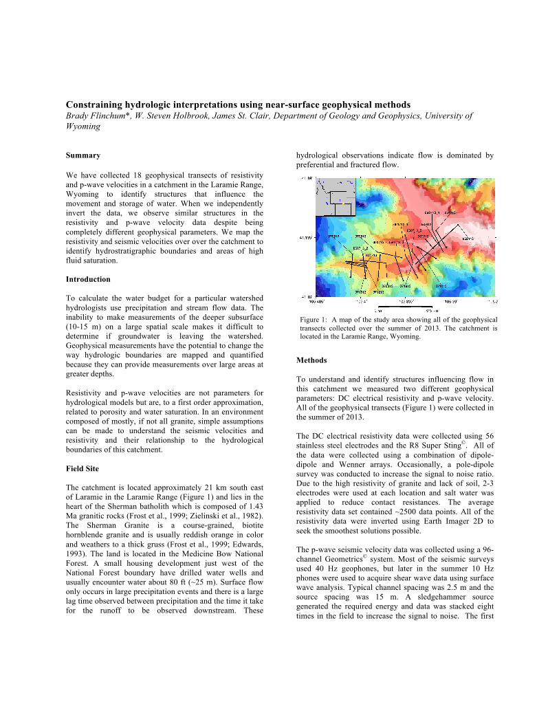
Methods To understand and identify structures influencing flow in this catchment we measured two different geophysical parameters: DC electrical resistivity and p-wave velocity. All of the geophysical transects (Figure 1) were collected in the summer of 2013. The DC electrical resistivity data were collected using 56 stainless steel electrodes and the R8 Super Sting©. All of the data were collected using a combination of dipole-dipole and Wenner arrays. Occasionally, a pole-dipole survey was conducted to increase the signal to noise ratio. Due to the high resistivity of granite and lack of soil, 2-3 electrodes were used at each location and salt water was applied to reduce contact resistances. The average resistivity data set contained ~2500 data points. All of the resistivity data were inverted using Earth Imager 2D to seek the smoothest solutions possible. The p-wave seismic velocity data was collected using a 96-channel Geometrics© system. Most of the seismic surveys used 40 Hz geophones, but later in the summer 10 Hz phones were used to acquire shear wave data using surface wave analysis. Typical channel spacing was 2.5 m and the source spacing was 15 m. A sledgehammer source generated the required energy and data was stacked eight times in the field to increase the signal to noise. The first

Figure 1: A map of the study area showing all of the geophysical transects collected over the summer of 2013. The catchment is located in the Laramie Range, Wyoming.

Constraining hydrologic interpretations using geophysics

arrivals were picked manually using Pickwin©. All of the velocity data were inverted using a shortest path algorithm (Dijkstra, 1959; Moser 1991). The inversion parameters were set to achieve smooth solutions. Results Due to the large amount of spatial data we are able plot the resistivity and seismic velocities over the entire catchment. Due to the shallow depth of our surveys (~20 – 30 m) we are unable to generate elevation slices because the total relief of the catchment is greater than 50 m. Instead we analyze p-wave velocity and resistivity at depths below the surface. The resistivity response of a material is a combination of the pore fluid and the mineralogy of the rock (Archie, 1941). If all of the material is resistive granite, we can interpret lower resistivity values as locations where the subsurface is saturated. The resistivity data (Figure 2) show a conductor following the stream and drainage bottom. The streams drawn in Figure 2 were derived from the 10 m DEM following the methods of Tarboton (1997). The DEM derived streams correspond with conductors in the resistivity data and visual evidence of surface streams. The conductive areas at shallow depths (Figure 2A-2B) occur at

topographically low points and correlate with the DEM derived streams. The seismic velocities are a function of effective pressure, porosity, mineralogy and critical porosity (Holbrook, 2014; Mindlin, 1949). When the velocities are high, the porosity is low and vice versa. When the seismic velocities are plotted over the catchment scale (Figure 3) there is a clear increase of velocity with depth. In particular, near the drainage bottoms we observed higher velocities, whereas under hill slopes the velocities stay slower until much deeper depths. Conclusions Preliminary geophysical work in this catchment illustrates the ability of near surface geophysics to spatially constrain hydrological interpretations on a qualitative level. We can identify areas of high saturation and hydrostratigraphic boundaries in a simple lithology. Further studies will include the use of geostatistics to spatially interpolate the data and build a hydrologic model to better understand how water moves through this small catchment.

Figure 2: Plotted resistivity values at given depths. The thick black line represents streams calculated from the DEM. All resistivities are plotted on a log scale. (A) 2 m depth, (B) 4 m depth, (C) 6 m depth and (D) 8 m depth.

Constraining hydrologic interpretations using geophysics

Figure 3: P-wave velocities at given depths. (A) 2 m depth, (B) 4 m depth, (C) 6 m depth and (D) 8 m depth.