constitutive models to simulate failure of structures made...
TRANSCRIPT

Ali E
dala
t Beh
baha
ni
janeiro de 2017UMin
ho |
201
7C
onst
itutiv
e M
odel
s to
Sim
ulat
e Fa
ilure
of
Stru
ctur
es M
ade
by C
emen
t Bas
ed M
ater
ials
Universidade do MinhoEscola de Engenharia
Ali Edalat Behbahani
Constitutive Models to Simulate Failure ofStructures Made by Cement Based Materials

janeiro de 2017
Tese de DoutoramentoPlano de tese no âmbito do Programa Doutoral emEngenharia Civil
Trabalho efectuado sob a orientação doProfessor Joaquim António Oliveira de Barros
e co-orientação doProfessor António Ventura Gouveia
Ali Edalat Behbahani
Constitutive Models to Simulate Failure ofStructures Made by Cement Based Materials
Universidade do MinhoEscola de Engenharia


iv

v
Dedicated To:
My family
Without their help, this work would not be possible.

vi

vii
ACKNOWLEDEMENTS
The research reported in the present thesis is carried out at the Department of Civil
Engineering of University of Minho. The financial supports provided by the research
projects “PREPAM” with reference number of PTDC/ECM/114511/2009, and “SlabSys-
HFRC”, with reference PTCD/ECM/120394/2010, both supported by the Portuguese
Foundation for Science and Technology (FCT), are gratefully acknowledged.
I would like to express my deepest gratitude to my supervisor Professor Joaquim Barros,
from University of Minho, as well as my co-supervisor Professor António Ventura-
Gouveia from Polytechnic Institute of Viseu, for their guidance and patience along these
years. They provided me continuous support for following my ideas and development of
the work presented here. To them, my sincerely thanks. It was a pleasure to work with
you!
My sincerely thanks also go to Doctor Eduardo Pereira, Doctor Rajendra Varma, Doctor
Omid Omidi, Doctor Ziad Taqieddin for their willingness to share their thoughts and
ideas.
I also dedicate my deeply thanks to all the secretarial staff for the completely unselfish
help on the bureaucratic issues.
I am very grateful to all my friends and colleagues in University of Minho for their
supports and sincere friendship during the execution of this work.
The days would have passed far more slowly without the support of my parents, Mrs.
Eshrat Yazdanjoo and Mr. Abolghasem Edalat Behbahani, who encourage me to be an
independent thinker, and having confidence in my abilities to go after new things that
inspired me. I also would like to thank my sister, Azin Edalat Behbahani, and my brother,
Ehsan Edalat Behbahani, for understanding and emotional supports. I sincerely thank my
family for their constant support, encouragement and patience while I was far from them
during these years. I am especially thankful to my parents-in-law, Ahmad Soltanzadeh
and Fahimeh Taban Kia, and my sister-in-law, Firoozeh Soltanzadeh, who provided me
with unending encouragement and support.

viii
Ali found love of his life, Faranak, at University of Minho. Thank you, Faranak, for all
the unconditional supports and sacrifices that you made.
Most importantly, I thank God for all His blessing to live this unmemorable experience.
Ali Edalat Behbahani
September 2016
ix
ABSTRACT
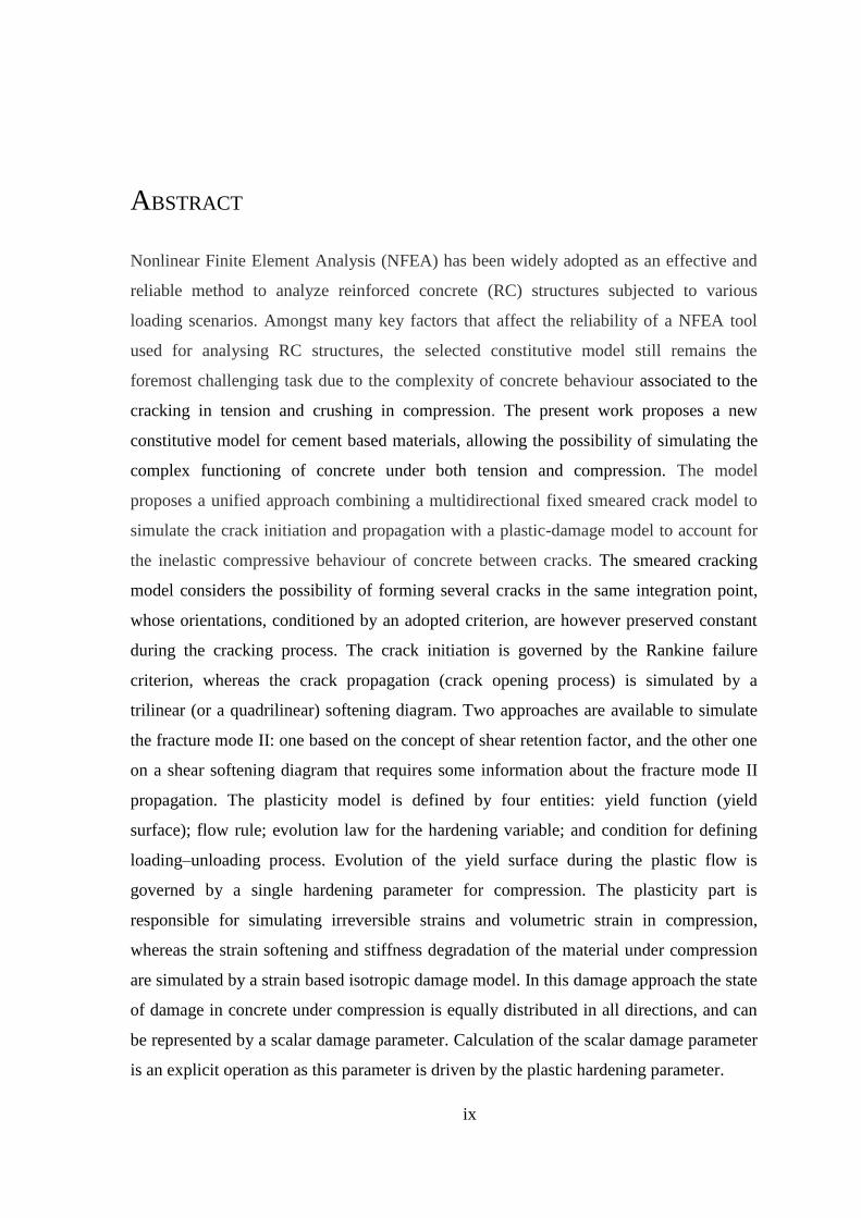
Nonlinear Finite Element Analysis (NFEA) has been widely adopted as an effective and
reliable method to analyze reinforced concrete (RC) structures subjected to various
loading scenarios. Amongst many key factors that affect the reliability of a NFEA tool
used for analysing RC structures, the selected constitutive model still remains the
foremost challenging task due to the complexity of concrete behaviour associated to the
cracking in tension and crushing in compression. The present work proposes a new
constitutive model for cement based materials, allowing the possibility of simulating the
complex functioning of concrete under both tension and compression. The model
proposes a unified approach combining a multidirectional fixed smeared crack model to
simulate the crack initiation and propagation with a plastic-damage model to account for
the inelastic compressive behaviour of concrete between cracks. The smeared cracking
model considers the possibility of forming several cracks in the same integration point,
whose orientations, conditioned by an adopted criterion, are however preserved constant
during the cracking process. The crack initiation is governed by the Rankine failure
criterion, whereas the crack propagation (crack opening process) is simulated by a
trilinear (or a quadrilinear) softening diagram. Two approaches are available to simulate
the fracture mode II: one based on the concept of shear retention factor, and the other one
on a shear softening diagram that requires some information about the fracture mode II
propagation. The plasticity model is defined by four entities: yield function (yield
surface); flow rule; evolution law for the hardening variable; and condition for defining
loading–unloading process. Evolution of the yield surface during the plastic flow is
governed by a single hardening parameter for compression. The plasticity part is
responsible for simulating irreversible strains and volumetric strain in compression,
whereas the strain softening and stiffness degradation of the material under compression
are simulated by a strain based isotropic damage model. In this damage approach the state
of damage in concrete under compression is equally distributed in all directions, and can
be represented by a scalar damage parameter. Calculation of the scalar damage parameter
is an explicit operation as this parameter is driven by the plastic hardening parameter.
x
Two versions of the model are developed, one dedicated to concrete structures subjected
to plane stress fields, and the second for being applied to concrete structures submitted to
three dimensional stress states. Both versions of the model are implemented into FEMIX
4.0 computer program. To appraise the performance of the model and to evidence the
interaction between cracking and plasticity-damage parts of the model, some numerical
tests at material level are executed, and the obtained results are discussed. The model
appraisal at the structural level is also considered. The set of experimental tests simulated
in this thesis covers a wide range of specimens regarding geometry, concrete type,
loading configurations, and reinforcement conditions, in order to demonstrate the
robustness of the developed model. These structures are of particular interest for the
assessment of the reliability of the model, since in these examples the failure mechanism
involved simultaneous occurrence of cracking and inelastic deformation in compression.
The predictive performance of the model in terms of load carrying capacity, ductility,
crack pattern, plastic zones, and failure modes is obtained by comparing the results of the
numerical simulations and the available experimental data.
Keywords: finite element analysis; plastic-damage multidirectional fixed smeared crack
model; compressive nonlinearity; cracked concrete; RC structures; cement based
materials.

xi
RESUMO
O método dos elementos finitos (MEF) tem-se revelado eficaz na análise não linear de
estruturas de betão armado submetidas a diferentes tipos de carregamentos. De entre os
muitos fatores que podem afetar a fiabilidade de uma ferramenta capaz de efetuar uma
análise não linear usando o MEF, o modelo constitutivo selecionado ainda continua a ser
o desafio mais importante, nomeadamente devido à complexidade do comportamento do
betão associado à fendilhação quando sujeito a tração e ao esmagamento em compressão.
O presente trabalho propõe um novo modelo constitutivo, capaz de simular o
comportamento complexo de materiais de matriz cimentícia quando sujeitos a esforços de
tração e de compressão. O modelo propõe uma abordagem unificada, combinando um
modelo de múltiplas fendas fixas distribuídas que permite simular o início de fendilhação
e a sua propagação com um modelo de dano e plasticidade para simular o comportamento
inelástico do betão entre fendas. O modelo de fendilhação permite a formação de várias
fendas por ponto de integração, cuja orientação é condicionada por um determinado
critério e preservada constante durante o processo de fendilhação. A abertura de fenda é
condicionada pelo critério de Rankine, sendo o seu desenvolvimento simulado por
intermédio de um diagrama de amolecimento trilinear ou quadrilinear. Duas abordagens
estão disponíveis para simular o modo II de fratura: uma baseada no conceito de fator de
retenção ao corte, e o outro utilizando um diagrama de amolecimento definido com base
nos parâmetros do modo II de fractura.
O modelo de plasticidade é definido: pela função de cedência (superfície de cedência); lei
de escoamento plástico; lei de endurecimento; condição para a definição do processo de
carga e descarga. A evolução da superfície de cedência durante o escoamento plástico é
governada por um único parâmetro de endurecimento. A parte da plasticidade é
responsável por simular as deformações irreversíveis e a deformação volumétrica em
compressão, enquanto o amolecimento e a degradação da rigidez do material sob
compressão são simulados por um modelo de dano isotrópico. Nesta abordagem, o estado
de dano no betão sob compressão é igualmente distribuído em todas as direções, e pode
ser representado por um escalar denominado parâmetro de dano.

xii
O modelo proposto é desenvolvido numa primeira fase para estados planos de tensão e
posteriormente generalizado para estados de tensão tridimensionais. Estas duas versões
do modelo foram integradas no código computacional denominado FEMIX 4.0. De forma
a evidenciar as partes do modelo que têm em conta a simulação da propagação da
fendilhação, do dano e da plasticidade, bem como da sua interação, são executados alguns
testes numéricos focados no comportamento do material, sendo os seus resultados
discutidos.
Os ensaios experimentais escolhidos para avaliar a robustez do modelo a nível estrutural
abrangem uma ampla gama de elementos no que respeita a geometria, tipo de betão,
configurações de carga e de reforço. Estas estruturas são de particular interesse para a
avaliação da fiabilidade do modelo, uma vez que nestes exemplos ocorrem
simultaneamente fendilhação e deformação plástica em compressão. O desempenho do
modelo em termos de previsão da capacidade de carga, da ductilidade, do padrão de
fendilhação, das zonas plásticas e dos modos de rutura é obtido comparando os resultados
das simulações numéricas com os dos ensaios experimentais disponíveis.

xiii
CONTENTS
ACKNOWLEDGEMENTS . . . . . . . . . . . . . . . . . . . . . . . . . . . . . . . . . . . . . . . . . vii
ABSTRACT . . . . . . . . . . . . . . . . . . . . . . . . . . . . . . . . . . . . . . . . . . . . . . . . . . . . ix
RESUMO . . . . . . . . . . . . . . . . . . . . . . . . . . . . . . . . . . . . . . . . . . . . . . . . . . . . . . . xi
CONTENTS . . . . . . . . . . . . . . . . . . . . . . . . . . . . . . . . . . . . . . . . . . . . . . . . . . . . xiii
LIST OF FIGURES . . . . . . . . . . . . . . . . . . . . . . . . . . . . . . . . . . . . . . . . . . . . . . . xix
LIST OF TABLES . . . . . . . . . . . . . . . . . . . . . . . . . . . . . . . . . . . . . . . . . . . . . . . . xxix
LIST OF SYMBOLS USED IN THE PROPOSED CONSTITUTIVE
MODELS. . . . . . . . . . . . . . . . . . . . . . . . . . . . . . . . . . . . . . . . . . . . . . . . . . . . . . . xxxiii
CHAPTER 1 - INTRODUCTION 1
1.1 MOTIVATION . . . . . . . . . . . . . . . . . . . . . . . . . . . . . . . . . . . . . . . . . . . . 1
1.2 SCOPES AND OBJECTIVES . . . . . . . . . . . . . . . . . . . . . . . . . . . . . . . . 2
1.3 OUTLINE OF THESIS . . . . . . . . . . . . . . . . . . . . . . . . . . . . . . . . . . . . . . 3
CHAPTER 2 – LITERATURE REVIEW 7
2.1 INTRODUCTION . . . . . . . . . . . . . . . . . . . . . . . . . . . . . . . . . . . . . . . . . . 7
2.2 MECHANICAL BEHAVIOUR OF CONCRETE . . . . . . . . . . . . . . . . . 7
2.2.1 Concrete behaviour under compression . . . . . . . . . . . . . . . . . . . 8
2.2.2 Concrete behaviour under tension. . . . . . . . . . . . . . . . . . . . . . . . 11

xiv
2.3 REVIEW OF THE THEORIES FREQUENTLY USED FOR
MODELLING THE MECHANICAL BEHAVIOUR OF CONCRETE 13
2.4 BASICS OF THE CONSTITUTIVE MODELS FREQUENTLY
USED FOR CONCRETE. . . . . . . . . . . . . . . . . . . . . . . . . . . . . . . . . . . . . 19
2.4.1 Discrete interface approach (DIA) . . . . . . . . . . . . . . . . . . . . . 19
2.4.2 Generalized finite element method (GFEM) . . . . . . . . . . . . . . . 24
2.4.3 Fixed smeared crack approach . . . . . . . . . . . . . . . . . . . . . . . . 27
2.4.4 Plasticity approach . . . . . . . . . . . . .. . . . . . . . . . . . . . . . . . . . . 29
2.5 CONCLUSIONS . . . . . . . . . . . . . . . . . . . . . . . . . . . . . . . . . . . . . . . . . 33
CHAPTER 3 – TWO DIMENSIONAL PLASTIC-DAMAGE
MULTIDIRECTIONAL FIXED SMEARED CRACK MODEL 35
3.1 INTRODUCTION . . . . . . . . . . . . . . . . . . . . . . . . . . . . . . . . . . . . . . . . . . 35
3.2 MULTIDIRECTIONAL FIXED SMEARED CRACK MODEL (SC
MODEL). . . . . . . . . . . . . . . . . . . . . . . . . . . . . . . . . . . . . . . . 35
3.3 PLASTIC-DAMAGE MULTIDIRECTIONAL FIXED SMEARED
CRACK MODEL (PDSC MODEL) . . . . . . . . . . . . . . . . . . . . . . . . . . . 41
3.3.1 Damage concept in the context of plastic-damage model . . . . . 42
3.3.2 Constitutive relationship for PDSC model . . . . . . . . . . . . . . . . 45
3.3.3 Plasticity model in effective stress space . . . . . . . . . . . . . . . . 46
3.3.3.1 Hardening law . . . . . . . . . . . . . . . . . . . . . . . . . . . . . 47
3.3.3.2 System of nonlinear equations . . . . . . . . . . . . . . . . 49
3.3.4 Coupling the plasticity and the SC models . . . . . . . . . . . . . . . . . 55
3.3.5 Isotropic damage law . . . . . . . . . . . . . . . . . . . . . . . . . . . . . . . 59
3.4 SIMULATIONS AT THE MATERIAL LEVEL . . . . . . . . . . . . . . . . . . 61

xv
3.5 CONCLUSIONS . . . . . . . . . . . . . . . . . . . . . .. . . . . . . . . . . . . . . . . . . 64
CHAPTER 4 – APPLICATION OF TWO DIMENSIONAL PDSC
MODEL IN STRUCTURAL ANALYSIS 66
4.1 INTRODUCTION . . . . . . . . . . . . . . . . . . . . . . . . . . . . . . . . . . . . . . . . . . 66
4.2 STRUCTURAL EXAMPLES . . . . . . . . . . . . . . . . . . . . . . . . . . . . . . . 67
4.2.1 Shear RC walls . . . . . . . . . . . . . . . . . . . . . . . . . . . . . . . . . . . . . 67
4.2.2 RC deep beams with openings . . . . . . . . . . . . . . . . . . . . . . . . . 75
4.2.3 Indirect (splitting) tensile test. . . . . . . . . . . . . . . . . . . . . . . . . . . . 84
4.2.4 RC short span beams . . . . . . . . . . . . . . . . . . . . . . . . . . . . . . . 91
4.2.5 Shear strengthened RC beams. . . . . . . . . . . . . . . . . . . . . . . . . . 97
4.2.5.1 Beam prototypes . . . . . . . . . . . . . . . . . . . . . . . . . 97
4.2.5.2 Material properties . . . . . . . . . . . . . . . . . . . . . . . . 99
4.2.5.3 Finite element modelling and constitutive laws for
the materials . . . . . . . . . . . . . . . . . . . . . . . . . . . . 100
4.2.5.4 Results and discussions . . . . . . . . . . . . . . . . . . . . 101
4.2.6 Effect of fiber dosage and prestress level on shear behavior of
RC beams . . . . . . . . . . . . . . . . . . . . . . . . . . . . . . . . . . . . . . . . .
107
4.3 CONCLUSIONS. . . . . . . . . . . . . . . . . . . . . . . . . . . . . . . . . . . . . . . . . . . 117
CHAPTER 5 – THREE DIMENSIONAL PDSC MODEL:
FORMULATION AND APPLICATION IN STRUCTURAL ANALYSIS 120
5.1 INTRODUCTION . . . . . . . . . . . . . . . . . . . . . . . . . . . . . . . . . . . . . . . . . . 120
5.2 MODEL DESCRIPTION . . . . . . . . . . . . . . . . . . . . . . . . . . . . . . . . . . . . 121
5.2.1 Part of the model corresponding to the cracking process . . . . . 121
5.2.2 Part of the model corresponding to the elasto-plasticity . . . . . . . 124
5.2.3 Part of the model corresponding to the damage process . . . . . . . 125

xvi
5.3 SIMULATIONS AT THE MATERIAL LEVEL . . . . . . . . . . . . . . . . . 126
5.4 SIMULATIONS AT THE STRUCTURAL LEVEL . . . . . . . . . . . . . . 130
5.4.1 RC columns subjected to different eccentric loadings. . . . . . . . . 130
5.4.2 RC beams made by different concrete strength classes. . . . . . . . 137
5.4.3 RC wall subjected to pure torsion . . . . . . . . . . . . . . . . . . . . . . . 143
5.5 PARAMETRIC STUDY FOR THE MODEL PARAMETERS . . . . . . . 149
5.5.1 Influence of cf . . . . . . . . . . . . . . . . . . . . . . . . . . . . . . . . . . . . 149
5.5.2 Influence of 1c . . . . . . . . . . . . . . . . . . . . . . . . . . . . . . . . . . . . . 151
5.5.3 Influence of ,f cG . . . . . . . . . . . . . . . . . . . . . . . . . . . . . . . . . . . . . 151
5.5.4 Influence of ,
cr
t p . . . . . . . . . . . . . . . . . . . . . . . . . . . . . . . . . . . 151
5.5.5 Influence of . . . . . . . . . . . . . . . . . . . . . . . . . . . . . . . . . . . . 152
5.5.6 Influence of ,f sG . . . . . . . . . . . . . . . . . . . . . . . . . . . . . . . . . . . . 153
5.6 CONCLUSIONS . . . . . . . . . . . . . . . . . . . . . . . . . . . . . . . . . . . . . . . . . . . 154
CHAPTER 6 - CONCLUSIONS AND FUTURE PERSPECTIVES 158
6.1 GENERAL CONCLUSIONS . . . . . . . . . . . . . . . . . . . . . . . . . . . . . . . . 158
6.2 RECOMMENDATIONS FOR FUTURE REASEARCH . . . . . . . . . . . 161
6.2.1 Creep model . . . . . . . . . . . . . . . . . . . . . . . . . . . . . . . . . . . . . . . 161
6.2.2 Numerical simulation of fire condition . . . . . . . . . . . . . . . . . . . 161
REFERENCES 164
ANNEXES
ANNEX A – GEOMETRIC REPRESENTAION OF STRESS
INVARIANTS . . . . . . . . . . . . . . . . . . . . . . . . . . . . . . . . . . . . . . . . . . . . 178
ANNEX B – EXTRACTING YIELD FUNCTION FROM FAILURE
CRITERION . . . . . . . . . . . . . . . . . . . . . . . . . . . . . . . . . . . . . . . . . . . . . . 180

xvii
ANNEX C – SIMULATION OF CYCLIC UNIAXIAL
COMPRESSIVE TEST . . . . . . . . . . . . . . . . . . . . . . . . . . . . . . . . . . . . . 186
ANNEX D – FIRST AND SECOND ORDER DERIVATIVES . . . . . . 188
ANNEX E – METHODOLOGY TO DERIVE COMPRESSIVE
FRACTURE ENERGY FROM EXPERIMENTAL DATA. . . . . . . . . . . 202

xviii

xix
LIST OF FIGURES
CHAPTER 1 - INTRODUCTION
1.1 Structure of the thesis . . . . . . . . . . . . . . . . . . . . . . . . . . . . . . . . . . . . . . . . . . . 5
CHAPTER 2 – LITERATURE RVERVIEW
2.1 Load-deformation behaviour of the cement based materials under uniaxial
compression (Shah et al., 1995) .. . . . . . . . . . . . . . . . . . . . . . . . . . . . . . .
8
2.2 Uniaxial compressive stress-strain curves for the concrete in different
strength (Wischers, 1978) . . . . . . . . . . . . . . . . . . . . . . . . . . . . . . . . . . . . . . 9
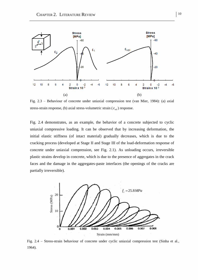
2.3 Behaviour of concrete under uniaxial compression test (van Mier, 1984):
(a) axial stress-strain response, (b) axial stress-volumetric strain ( vol )
response.. . . . . . . . . . . . . . . . . . . . . . . . . . . . . . . . . . . . . . . . . . . . . . .
10
2.4 Stress-strain behaviour of concrete under cyclic uniaxial compression test
(Sinha et al., 1964). . . . . . . . . . . . . . . . . . . . . . . . . . . . . . . . . . . . . . . . . . . 10
2.5 Basic fracture modes (Wang, 1996) . . . . . . . . . . . . . . . . . . . . . . . . . . . . . . . 11
2.6 Cyclic uniaxial tensile loading test (Reinhardt, 1984) . . . . . . . . . . . . . . . . 12
2.7 Cyclic uniaxial tensile-compressive loading test (Reinhardt, 1984) . . . . . . 13
2.8 Schematic unloading responses according to three approaches (Jason et
al., 2006): (a) damage model, (b) plasticity model, (c) plastic-damage
model (Note: in this figure the parameter E is the initial elastic stiffness,
and the parameter d is an scalar representing the state of damage in the
material) . . . . . . . . . . . . . . . . . . . . . . . . . . . . . . . . . . . . . . . . . . . . . . . . .
18
2.9 Domain crossed by a discontinuity d (Wells and Sluys, 2001) . . . . . . 20
2.10 Zero thickness interface elements with n pars of nodes with indication of
local (s, n) and global (x1, x2) coordinate systems (Malvern, 1969; Dias-
da-Costa 2010) . . . . . . . . . . . . . . . . . . . . . . . . . . . . . . . . . . . . . . . . . . . .
22
2.11 Propagation of discontinuity in GFEM (Dias-da-Costa 2010) . . . . . . . . . . 25

xx
CHAPTER 3 – TWO DIMENSIONAL PLASTIC-DAMAGE
MULTIDIRECTIONAL FIXED SMEARED CRACK MODEL
3.1 Diagrams for modelling the fracture mode I at the crack coordinate
system: (a) trilinear diagram (Sena-Cruz, 2004), (b) quadrilinear diagram
(Salehian and Barros, 2015). . . . . . . . . . . . . . . . . . . . . . . . . . . . . . . . . . . . .
38
3.2 Diagram for modelling the fracture mode II at the crack coordinate system
(Ventura-Gouveia, 2011) . . . . . . . . . . . . . . . . . . . . . . . . . . . . . . . . . . . . . . . 40
3.3 Relation between crack shear stress and crack shear strain for the
incremental approach based on a shear retention factor (Barros et al.,
2011) . . . . . . . . . . . . . . . . . . . . . . . . . . . . . . . . . . . . . . . . . . . . . . . . . . 41
3.4 One dimensional representation of the effective and nominal stresses
(Abu Al-Rub and Kim, 2010) . . . . . . . . . . . . . . . . . . . . . . . . . . . . . . . . . . . 43
3.5 Schematic representation of damage evolution in the proposed model . . . . 44
3.6 Diagrams for modelling the concrete compression behaviour: (a) the
c c relation used in the plasticity model; (b) the (1 )c dd relation
adopted in the isotropic damage model; (c) the (1 )c c cd diagram for
compression with indication of the compressive fracture energy, ,f cG . . .
49
3.7 Experimental (Kupfer et al., 1969) vs. predicted stress-strain response of
concrete under monotonic uniaxial compressive test: (Values for the
parameters of the constitutive model: poison’s ratio, =0.2; young’s
modulus, E=27 GPa; compressive strength, cf =32 MPa; strain at
compression peak stress 1c =0.0023; parameter to define elastic limit
state 0 =0.3; compressive fracture energy,
,f cG =15.1 N/mm) . . . . . . . .
62
3.8 Experimental (Karsan and Jirsa, 1969) vs. predicted stress-strain response
of concrete under cyclic uniaxial compressive test: (Values for the
parameters of the constitutive model: =0.2; E=27 GPa; 0 =0.3;
1c
=0.0017; cf =28 MPa;
,f cG =11.5 N/mm) . . . . . . . . . . . . . . . . . . . . . . . . .
63
3.9 Prediction of the PDSC model for closing a crack developed in one
direction, by imposing compressive load in the orthogonal direction
(Values for the parameters of the constitutive model: =0.2; E=36 GPa;
cf =30 MPa; ,f cG =30 N/mm;
1c =0.0022; 0 =0.3;
ctf =2.45 MPa; I
fG
=0.05 N/mm; 1 =0.2;
1 =0.7; 2 =0.75;
2 =0.2.. . . . . . . . . . . . . . . . . . . .
64
xxi
CHAPTER 4 – APPLICATION OF TWO DIMENSIONAL PDSC
MODEL IN STRUCTURAL ANALYSIS
4.1 Geometry and loading configurations of the shear walls tested by Maier
and Thürlimann (1985) (dimensions in mm): (a) the walls in group A
(with vertical flange); (b) the walls in group B (without vertical flange). . . 68
4.2 Simulation of the S4 shear wall tested by Maier and Thürlimann (1985):
(a) finite element mesh used for the analysis; (b) horizontal load vs.
horizontal displacement diagram, Fh-Uh; (c) experimentally observed
crack pattern (Maier and Thürlimann, 1985); (d) crack pattern and (e)
plastic zone (results of (d) and (e) correspond to 18hU mm , the final
converged step, for the simulation using ,f cG =30 N/mm) (Notes: (1) - In
pink color: crack completely open; in red color: crack in the opening
process; in cyan color: crack in the reopening process; in green color:
crack in the closing process; in blue color: closed crack; in red circle: the
plastic zone; (2) - The crack pattern and plastic zone are represented over
the finite element mesh adopted for the concrete) . . . . . . . . . . . . . . . . . . . .
70
4.3 Uniaxial constitutive model (for both tension and compression) for the
steel bars (Sena-Cruz, 2004) . . . . . . . . . . . . . . . . . . . . . . . . . . . . . . . . . . . . 71
4.4 Sensitivity of the analysis of the panel S4 respect to the size of finite
element mesh: (a) refined finite element mesh used for analysis; (b) Fh-Uh
relationship; (c) Numerical crack pattern obtained at final converged step
of the analysis. Note: the crack pattern is represented over the finite
element mesh adopted for the concrete.. . . . . . . . . . . . . . . . . . . . . . . . .
73
4.5 Simulation of the shear walls S1, S2, S3, S9, S10 tested by Maier and
Thürlimann (1985): (a) horizontal load vs. horizontal displacement
relationship, Fh-Uh; (b) numerical crack pattern predicted by PDSC model
and corresponding to the final converged step; (c) experimentally
observed crack pattern (Maier and Thürlimann, 1985). Note: the crack
pattern is represented over the finite element mesh adopted for the
concrete . . . . . . . . . . . . . . . . . . . . . . . . . . . . . . . . . . . . . . . . . . . . . . . . .
74
4.6 Deep beams with openings tested by El-Maaddawy and Sherif (2009): (a)
details of the reinforcement system, common for all the beams in the
experimental program; (b) geometry of the beams at group B, NS-200-B
and NS-250-B; (c) geometry of the beams at group T, NS-200-T and NS-
250-T; (d) geometry of the beams at group C, NS-200-C and NS-250-C . .
77

xxii
4.7 Finite element mesh, load and support conditions used for analysis of the
beam NS-200-C. . . . . . . . . . . . . . . . . . . . . . . . . . . . . . . . . . . . . . . . . . . . . . 78
4.8 Experimental load vs. mid-span deflection (El-Maaddawy and Sherif,
2009) in compare with the predictions of the PDSC and SC models for the
beams: (a) NS-200-B; (b) NS-200-T; (c) NS-200-C; (d) NS-250-B; (e)
NS-250-T; (f) NS-250-C. . . . . . . . . . . . . . . . . . . . . . . . . . . . . . . . . . . . .
80
4.9 Experimental crack patterns (El-Maaddawy and Sherif, 2009) for the
beams: (a) NS-200-B; (b) NS-200-T; (c) NS-250-B; (d) NS-250-T; (e)
NS-250-C . . . . . . . . . . . . . . . . . . . . . . . . . . . . . . . . . . . . . . . . . . . . . . . . 81
4.10 Numerical crack patterns (left) and plastic zones (right) predicted by
PDSC model for the beams in analysis (the results correspond to the final
converged step). Note: the crack pattern and plastic zone are represented
over the finite element mesh adopted for the concrete. . . . . . . . . . . . . . . . .
82
4.11 Details of the splitting tensile test: (a) setup of the test (Abrishambaf et
al., 2015); (b) geometry of the specimen, dimensions are in mm; (c)
experimental crack pattern at the failure stage (Abrishambaf, 2015) . . . . . 84
4.12 Finite element mesh, load and support conditions used for analysis of the
splitting tensile test. . . . . . . . . . . . . . . . . . . . . . . . . . . . . . . . . . . . . . . . . . 85
4.13 Experimental load vs. crack mouth opening displacement relationship
Abrishambaf et al. (2013) in comparison with the predictions of the PDSC
and SC models. . . . . . . . . . . . . . . . . . . . . . . . . . . . . . . . . . . . . . . . . . . . 86
4.14 Predictions of PDSC model for the splitting tensile test: (a) numerical
crack pattern; (b) numerical plastic zone (results of (a) and (b) correspond
to 1.9W mm, the final converged loading step). . . . . . . . . . . . . . . . . . . . . 87
4.15 Cube splitting tensile test: (a) coarse mesh; (b) fine mesh (dimensions in
mm) . . . . . . . . . . . . . . . . . . . . . . . . . . . . . . . . . . . . . . . . . . . . . . . . . . . . 89
4.16 Stress vs. vertical displacement under the load predicted by PDSC model
for the cube splitting tensile test . . . . . . . . . . . . . . . . . . . . . . . . . . . . . . . 90
4.17 Numerical crack pattern obtained by PDSC model for cube splitting
tensile test: (a) coarse mesh; (b) fine mesh (results correspond to the final
converged loading step) . . . . . . . . . . . . . . . . . . . . . . . . . . . . . . . . . . . . .
90
4.18 Numerical plastic zone obtained by PDSC model for cube splitting tensile
test: (a) coarse mesh; (b) fine mesh (results correspond to the final
91

xxiii
converged loading step) . . . . . . . . . . . . . . . . . . . . . . . . . . . . . . . . . . . . . . . .
4.19 Beam configuration and test setup (dimensions in mm) (Soltanzadeh et
al., 2016a) . . . . . . . . . . . . . . . . . . . . . . . . . . . . . . . . . . . . . . . . . . . . . . . . . . . 91
4.20 Finite element mesh used for the simulated beams (dimensions in mm) . . 93
4.21 Numerical prediction of the applied load vs. mid-span deflection in
comparison with the corresponding experimental results of the beam
series: (a) Bi-P0; (b) Bi-P20; (c) Bi-P30. . . . . . . . . . . . . . . . . . . . . . . . . . . . 94
4.22 Crack patterns predicted by the model (a) and crack patterns obtained in
the experimental tests (b) for the beam series: Bi-P0; Bi-P20; Bi-P30.. . . . 95
4.23 Strain in steel reinforcement (obtained at the closest IP to the symmetric
axis of the beam) vs. mid-span deflection predicted by the numerical
simulations.. . . . . . . . . . . . . . . . . . . . . . . . . . . . . . . . . . . . . . . . . . . . . . . 96
4.24 The predicted load-deformation behavior for all the beam series. . . . . . . . . 96
4.25 Geometry of the reference beam (3S-R), steel reinforcements common to
all beams, support and load conditions (dimensions in mm) (Barros and
Dias, 2013). . . . . . . . . . . . . . . . . . . . . . . . . . . . . . . . . . . . . . . . . . . . . . . . 97
4.26 NSM shear strengthening configurations (CFRP laminates at dashed lines;
dimensions in mm) (Barros and Dias, 2013) . . . . . . . . . . . . . . . . . . . . . . . . 98
4.27 Finite element mesh used for the beam 3S-4LI-S2 (dimensions are in
mm). . . . . . . . . . . . . . . . . . . . . . . . . . . . . . . . . . . . . . . . . . . . . . . . . . . . . 100
4.28 Experimental (Barros and Dias, 2013) and numerical load vs. the
deflection at loaded deflection: (a) 3S-R; (b) 3S-4LI-S2; (c) 3S-4LI-P2;
(d) 3S-4LI4LI-SP1; (e) 3S-4LI4LV-SP1. . . . . . . . . . . . . . . . . . . . . . . . .
103
4.29 Crack patterns of the tested beams at failure (Barros and Dias, 2013) . . . . 104
4.30 Crack patterns and plastic zones predicted by PDSC model for the beams:
(a) 3S-R; (b) 3S-4LI-S2; (c) 3S-4LI-P2; (d) 3S-4LI4LI-SP1; (e) 3S-
4LI4LV-SP1 (the results are correspondent to the final converged step) . . 104
4.31 Experimental and numerical presentations of load-strain diagram for the
beam 3S-4LI-S2: (a) monitored laminates; (b) NSM laminate A; (c) NSM
laminate B; (e) monitored still stirrup . . . . . . . . . . . . . . . . . . . . . . . . . . . . .
106

xxiv
4.32 Geometry, reinforcement and test setup of the beams of (a) group 1 (G1-
F1.1-S0; G1-F1.1-S23; G1-F1.1-S46), (b) group 2 except G2-F0-ST, (c)
G2-F0-ST (dimensions in mm) (Soltanzadeh et al., 2016b) . . . . . . . . . . . . 107
4.33 Finite element mesh, load and support conditions used for analysis of the
beam G1-F1.1-S0 . . . . . . . . . . . . . . . . . . . . . . . . . . . . . . . . . . . . . . . . . . . . . 109
4.34 Experimental and numerical load vs. mid-span deflection of the beams of
the first group: (a) G1- F1.1-S0; (b) G1- F1.1-S23; (c) G1- F1.1-S46 . . . . 112
4.35 Experimental and numerical load vs. mid-span deflection of the beams of
the second group: (a) G2- F0; (b) G2- F0-ST; (c) G2- F1.1; (d) G2-F1.5 . . 113
4.36 Crack pattern at failure of the first and second group of beams
(Soltanzadeh et al., 2016b).. . . . . . . . . . . . . . . . . . . . . . . . . . . . . . . . . . . . . 113
4.37 Numerical crack pattern predicted by PDSC model for the beam G2- F1.5
(The results correspond to the final converged step) . . . . . . . . . . . . . . . . . . 114
4.38 Experimental and numerical load vs. strain in steel stirrups of beam G2-
F0-ST . . . . . . . . . . . . . . . . . . . . . . . . . . . . . . . . . . . . . . . . . . . . 114
4.39 Experimental and numerical load vs. GFRP strain at mid-span of the
beams . . . . . . . . . . . . . . . . . . . . . . . . . . . . . . . . . . . . . . . . . . . . . . . . . . 115
4.40 Numerical load vs. strain of strand in mid-span of the beams relationships
. . . . . . . . . . . . . . . . . . . . . . . . . . . . . . . . . . . . . . . . . . . . . . . . . . . . . . . . . 116
CHAPTER 5 – THREE DIMENSIONAL PDSC MODEL:
FORMULATION AND APPLICATION IN STRUCTURAL ANALYSIS
5.1 Crack stress components, displacements and local coordinate system of
the crack (Ventura-Gouveia et al., 2008; Ventura-Gouveia, 2011) . . . . . . . 122
5.2 Simulation of cyclic compression-tension load sequence at the material
level (values for the parameters of the constitutive model: =0.2; E =22
GPa; cf =30 MPa; ,f cG =7 N/mm; ctf =3 MPa; 1c =0.0025; 0 =0.3;
fG
=0.04 N/mm; 1 =0.2; 1 =0.7; 2 =0.75; 2 =0.2) . . . . . . . . . . . . . . . . . . .
127
5.3 Prediction of the PDSC model for closing a crack developed in one
direction, by imposing compressive load in the orthogonal direction
(values for the parameters of the constitutive model: =0.2; E =36 GPa;

xxv
cf =30 MPa; ,f cG =30 N/mm; ctf =2.45 MPa; 1c =0.0025; 0 =0.3;
fG
=0.05 N/mm; 1 =0.2; 1 =0.7; 2 =0.75; 2 =0.2) . . . . . . . . . . . . . . . . . . . 128
5.4 Prediction of the PDSC model for closing two cracks developed along
two orthogonal directions, by imposing compressive load in the third
orthogonal direction (values for the parameters of the constitutive model
adopted the same as those mentioned in Fig. 5.3). . . . . . . . . . . . . . . . . . . . .
130
5.5 Details of the test specimen (El-Maaddawy, 2009) (dimensions in mm) . . 131
5.6 Test set up (El-Maaddawy, 2009) . . . . . . . . . . . . . . . . . . . . . . . . . . . . . . . . 132
5.7 Finite element mesh used for the simulation of the column C-e0.86: (a)
concrete and steel plates; (b) reinforcements . . . . . . . . . . . . . . . . . . . . . 133
5.8 Experimental vs. numerical P-Uh responses (El-Maaddawy, 2009) for the
specimen: (a) C-e0.3; (b) C-e0.57; (c) C-e0.86 . . . . . . . . . . . . .. . . . . . . . . 134
5.9 Experimental vs. numerical ,r tP responses (El-Maaddawy, 2009) for
the specimen: (a) C-e0.3; (b) C-e0.57; (c) C-e0.86 . . . . . . . . . . . . . . . . . . . 135
5.10 Results of the specimen C-e0.3: (a) experimentally observed damage (El-
Maaddawy, 2009); (b) numerical crack pattern and (c) plastic zone
(results of (b) and (c) correspond to the last converged step ( 9.2hU mm )
. . . . . . . . . . . . . . . . . . . . . . . . . . . . . . . . . . . . . . . . . . . . . . . . . . . . . . . . 136
5.11 Geometry and reinforcement layout for the beams tested by Yang et al.
(2003) (dimensions in mm) . . . . . . . . . . . . . . . . . . . . . . . . . . . . . . . . . . . . . 137
5.12 Finite element mesh used for the simulation of the beam L-75 (due to
symmetry conditions only half beam was modelled) . . . . . . . . . . . . . . . . . . 139
5.13 Experimental (Yang et al., 2003) and numerical load versus the mid-span
deflection for the beams: (a) L-60; (b) L-75; (c) L-100; (d) H-60; (e) H-
75; (f) H-100. . . . . . . . . . . . . . . . . . . . . . . . . . . . . . . . . . . . . . . . . . . . . .
141
5.14 Results of the beam H-60: (a) experimental crack patterns; (b) numerical
crack pattern; (c) plastic zone (for (b) and (c) the damage stages are
obtained at the last converged step) . . . . . . . . . . . . . . . . . . . . . . . . . . . . . . . 142
5.15 General arrangement of the wall specimens tested by Peng and Wong
(2011) (dimensions in mm).. . . . . . . . . . . . . . . . . . . . . . . . . . . . . . . . . . . . . 144

xxvi
5.16 Setup for the test of shear walls subjected to torsion (Peng and Wong,
2011) . . . . . . . . . . . . . . . . . . . . . . . . . . . . . . . . . . . . . . . . . . . . . . . . . . . 145
5.17 Finite element mesh used for the simulation of the wall S10 . . . . . . . . . . . 146
5.18 Experimental (Peng and Wong, 2011) and numerical torque-twist angle
per length for: (a) the wall S8; (b) the wall S10 . . . . . . . . . . . . . . . . . . . . . . 148
5.19 Results of the S8 wall: (a) experimentally observed crack pattern (Peng
and Wong, 2011); (b) numerically predicted crack pattern, obtained at the
last converged step. Note: the numerical crack pattern is represented over
the finite element mesh adopted for concrete, i.e., the finite element mesh
adopted for the reinforcement is hidden.. . . . . . . . . . . . . . . . . . . . . . . . . . .
148
5.20 Sensitivity of the analysis of the beam L-75 with respect to the values of
the parameters: (a) cf ; (b)
1c ; (c) ,f cG .. . . . . . . . . . . . . . . . . . . . . . . . . 150
5.21 Sensitivity of the analysis of the S10 wall with respect to the value of the
parameter ,
cr
t p .. . . . . . . . . . . . . . . . . . . . . . . . . . . . . . . . . . . . . . . . . . . . 152
5.22 Sensitivity of the analysis of the S10 wall with respect to the value of the
parameter . . . . . . . . . . . . . . . . . . . . . . . . . . . . . . . . . . . . . . . . . . . . . 153
5.23 Sensitivity of the analysis of the S10 wall with respect to the value of the
parameter ,f sG . . . . . . . . . . . . . . . . . . . . . . . . . . . . . . . . . . . . . . . . . . . . . . 154
ANNEX A – GEOMETRIC REPRESENTAION OF STRESS
INVARIANTS
A.1 Haigh-Westergaard stress space (Grassl et al., 2002) . . . . . . . . . . . . . . . . . 179
ANNEX B – EXTRACTING YIELD FUNCTION FROM
FAILURE CRITERION
B.1 Willam-Warnke failure surface represented in (a) meridian plane; (b)
deviatoric plane (1 ,
2 ,3 are the principle effective stresses) . . . . . . . 180
ANNEX C – SIMULATION OF CYCLIC UNIAXIAL
COMPRESSIVE TEST
C.1 Cyclic uniaxial compressive test of Karsan and Jirsa (1969) ; (a) the
c c law of the model, (b) Experimental (Karsan and Jirsa, 1969) vs.

xxvii
predicted stress-strain response (assuming 0l =4.5) . . . . . . . . . . . . . . . . . . . 187
ANNEX E – METHODOLOGY TO DERIVE COMPRESSIVE
FRACTURE ENERGY FROM EXPERIMENTAL DATA
E.1 Set up of uniaxial compression test (Cunha, 2010) . . . . . . . . . . . . . . . . . . . 202
E.2 Model for determination of inel . . . . . . . . . . . . . . . . . . . . . . . . . . . . . . . . . . 204

xxviii

xxix
LIST OF TABLES
CHAPTER 4 – APPLICATION OF TWO DIMENSIONAL PDSC
MODEL IN STRUCTURAL ANALYSIS
4.1 Details for the shear wall panels . . . . . . . . . . . . . . . . . . . . . . . . . . . . . . . . . 69
4.2 Values of the parameters of the steel constitutive model for the shear walls tests. 70
4.3 Values of the parameters of the concrete constitutive model for shear wall
test . . . . . . . . . . . . . . . . . . . . . . . . . . . . . . . . . . . . . . . . . . . . . . . . . . . . . . . . 71
4.4 Details for the deep beam tests . . . . . . . . . . . . . . . . . . . . . . . . . . . . . . . . . . . 76
4.5 Values of the parameters of the steel constitutive model for deep beams
tests . . . . . . . . . . . . . . . . . . . . . . . . . . . . . . . . . . . . . . . . . . . . . . . . . . . . . . 78
4.6 Values of the parameters of the concrete constitutive model for the deep
beam (with openings) test . . . . . . . . . . . . . . . . . . . . . . . . . . . . . . . . . . . . . 79
4.7 Values of the parameters of the concrete constitutive model for the test of
cylinder splitting specimen made of SFRSCC . . . . . . . . . . . . . . . . . . . . . . . 86
4.8 Values of the parameters of the concrete constitutive model for the test of
cube splitting specimen made of plain concrete . . . . . . . . . . . . . . . . . . . . . 88
4.9 General information about the simulation of the prestress load by means
of temperature variation . . . . . . . . . . . . . . . . . . . . . . . . . . . . . . . . . . . . . . 92
4.10 Mechanical properties of the GFRP bar . . . . . . . . . . . . . . . . . . . . . . . . . . . . . . 93
4.11 Values of the parameters of the steel constitutive model for short beams
tests . . . . . . . . . . . . . . . . . . . . . . . . . . . . . . . . . . . . . . . . . . . . . . . . . . . . 93
4.12 Values of the parameters of the concrete constitutive model for the test of
short span beams . . . . . . . . . . . . . . . . . . . . . . . . . . . . . . . . . . . . . . . . . . 94
4.13 CFRP shear strengthening configurations of the tested beams . . . . . . . . . 100

xxx
4.14 Values of the parameters of the steel constitutive model for test of the
shear strengthened RC beams . . . . . . . . . . . . . . . . . . . . . . . . . . . . . . . . . . . 101
4.15 Values of the parameters of the concrete constitutive model for the test of
the shear strengthened RC beams . . . . . . . . . . . . . . . . . . . . . . . . . . . . . . . . 102
4.16 Details of the beams in first and second group . . . . . . . . . . . . . . . . . . . . 109
4.17 Values of the parameters of the steel constitutive model . . . . . . . . . . . . . . . 110
4.18 General information about the simulation of the prestress load by means
of temperature variation . . . . . . . . . . . . . . . . . . . . . . . . . . . . . . . . . . . . . 110
4.19 Values of the parameters of the concrete constitutive model for concretes
SCC-F0, SCC-F1.1, and SCC-F1.5 . . . . . . . . . . . . . . . . . . . . . . . . . . . . . . . 111
4.20 Details of the experimental results and the numerical analysis . . . . . . . . . . 115
CHAPTER 5 – THREE DIMENSIONAL PDSC MODEL:
FORMULATION AND APPLICATION IN STRUCTURAL ANALYSIS
5.1 Values of the parameters of the steel constitutive model for the tests with
RC column subjected to eccentric loading . . . . . . . . . . . . . . . . . . . . . . . . 133
5.2 Values of the parameters of the concrete constitutive model for the tests
with RC column subjected to eccentric loading . . . . . . . . . . . . . . . . . . . . . . 133
5.3 Details of the beams tested by Yang et al. (2003) . . . . . . . . . . . . . . . . . . . . . . . 138
5.4 Values of the parameters of the steel constitutive model for modelling the
beams tested by Yang et al. (2003) . . . . . . . . . . . . . . . . . . . . . . . . . . . . 139
5.5 Values of the parameters of the concrete constitutive model for simulating
the beams tested by Yang et al. (2003) . . . . . . . . . . . . . . . . . . . . . . . . . . . . 140
5.6 Experimental and numerical failure loads of the beams. . . . . . . . . . . . . . . . 143
5.7 Details of the RC walls submitted to torsion . . . . . . . . . . . . . . . . . . . . . . . . 144
5.8 Values of the parameters of the steel constitutive model for the test of RC
walls . . . . . . . . . . . . . . . . . . . . . . . . . . . . . . . . . . . . . . . . . . . . . . . . . . . . . . . 147
5.9 Values of the parameters of the concrete constitutive model for the test of
RC walls . . . . . . . . . . . . . . . . . . . . . . . . . . . . . . . . . . . . . . . . . . . . . . . . . . . . 147

xxxi
ANNEX B
B.1 Experimental failure points to determine the constants of tensile meridian 182

xxxii

xxxiii
LIST OF SYMBOLS USED IN THE PORPOSED CONSTITUTIVE
MODELS
effective stress vector at global coordinate system
nominal stress vector at global coordinate system
eD linear elastic constitutive matrix
the positive component, corresponding to tensile state of stress, of stress
vector
the negative component, corresponding to compressive state of stress, of
stress vector
i ith principle stress extracted from the vector
iP the normalized eigenvector associated with the ith principle stress i
cr incremental crack strain vector
co incremental concrete strain vector
incremental total strain vector
p incremental plastic strain vector
i orientation corresponding to the i-th crack
IP integration point
cr incremental crack strain vector at crack coordinate system
cr incremental stress vector at crack coordinate system
cr
n normal components of the local crack stress vector
cr
t shear components of the local crack stress vector
cr
n normal components of the local crack strain vector

xxxiv
cr
t shear components of the local crack strain vector
crT transformation matrix from the coordinate system of the finite element to the
local crack coordinate system
crD crack constitutive matrix
cr
nD the stiffness modulus correspondent to the fracture mode I
cr
tD the stiffness modulus correspondent to the fracture mode II
E modulus of elasticity
Poisson’s coefficient
i normalized stress parameters (i=1, 2) in trilinear diagram
shear retention factor
i normalized strain parameter (i =1, 2) in trilinear diagram
cf compressive strength of concrete
ctf tensile strength of concrete
cG elastic shear modulus
If
G mode I fracture energy
,f sG mode II fracture energy
,f cG compressive fracture energy
bl crack bandwidth
cl Compressive characteristic length which was assumed identical to the crack
bandwidth
,
cr
n u ultimate crack normal strain
1P parameter that defines the amount of the decrease of upon increasing cr
n
,
cr
t p peak crack shear strain
,crt p peak crack shear stress
,
cr
t u ultimate crack shear strain

xxxv
1I first invariant of the effective stress tensor
2J second invariant of the deviatoric effective stress tensor
3J third invariant of deviatoric eddective stress tensor
angle of similarity
hydrostatic stress invariant
deviatoric stress invariants
, ,a b c parameters of Willam-Warnke yield surface depending to state of stress
c hardening function of the plasticity model
1c strain at compression peak stress
( , )cf yield function
c compressive hardening variable
plastic multiplier
1c accumulated plastic strain at uniaxial compressive peak stress
0cf uniaxial compressive stress at plastic threshold
0 material constant to define the beginning of the nonlinear behaviour in
uniaxial compressive stress-strain test
cd scalar describing the amount compressive damage
d internal damage variable for compression
ca non-dimensional parameter of damage
, ,sy sh su three strain points at the steel constitutive law
, ,sy sh su three stress points at the steel constitutive law
P parameter that defines the shape of the last branch of the steel stress-strain
curve

xxxvi
syE unloading-reloading slop for the steel constitutive law

C H P A T E R 1
INTRODUCTION
1.1 MOTIVATION
Concrete is known as one of the most widely used construction material in civil
engineering. The main advantages of concrete are: high workability and formability that
allows its application to various structural elements in buildings, bridges, dams, etc; high
durability in severe environmental condition; it is a relatively cheap material with a few
maintenance requirements; fire resistance of reinforced concrete (RC) structures, since
concrete bulk limits the elevation of temperature in the reinforcement rebars. However,
concrete exhibits highly nonlinear behaviour by increasing deformation, with
dissymmetric responses in tension and in compression (i.e. concrete has relatively low
tensile strength when compared to its compressive strength).
Since the advent of concrete, the analysis and design of concrete structures have been
objective of many researchers and designers. The development of computer oriented FEM
(finite element method) based numerical models for two- and three- dimensional
structural analysis contributed much to the possibility of calculating nowadays concrete
structures with complex/arbitrary geometry. Analysis of structural engineering problems
by FEM is based on solution of a set of equilibrium equations between the internal forces
(those supported by the consitituent materials of the structure) and the external ones
(combination of load cases). To determine with appropriate accuracy the internal forces,

CHAPTER 1. INTRODUCTION 2
the FEM-based approach must take into consideration the strain/stress limits capable of
supporting by the materials. The physical/mathematical representation of these limits
simulates the behaviour of a material, and is generally designated by the “material
constitutive model”. Many constitutive models, from simple to sophisticated, have been
developed for material nonlinear analysis of RC structures. However, during the course of
these developments, modelling of concrete structures has always proven to be a
challenge, particularly due to the complexity of concrete behaviour. Concrete exhibits
highly nonlinear behaviour by increasing deformation, with dissymmetric responses in
tension and in compression. Experimental tests demonstrate that concrete behaviour in
tension is brittle, and after cracking initiation it develops a softening behaviour with a
decay of tensile capacity with the widening of the cracks. This crack opening process is
followed by a decrease of crack shear stress transfer due to the deterioration of aggregate
interlock. Concrete in compression also exhibits a pronounced nonlinear behaviour with
an inelastic irreversible deformation. In the pre-peak stage of concrete response in
uniaxial compression, a nonlinear stage is observed, whose amplitude depends of the
concrete strength class, followed by a softening stage where brittleness is also dependent
of the strength class. The complexity of concrete behaviour increases when submitted to
multiaxial stress field that is the current situation of the major RC structures. For a
realistic Nonlinear Finite Element Analysis (NFEA) of RC structures, constitutive models
are required to adequately describe these complex behaviours of concrete.
One possible theoretical framework to develop a constitutive model capable of simulating
both dissymmetric responses of concrete under tension and compression, is coupling a
fracture approach to the plasticity theory. In this class of models, the theory of plasticity
is used to deal with the elastoplastic behaviour of material under compression, whereas
various fracture theories can be used to simulate the cracking behaviour (de Borst, 1986;
Cervenka and Papanikolaou, 2008). However, numerical difficulties may occur with this
class of models when applied to simulate structures whose failure is governed,
simultaneously, by cracking and inelastic behaviour in compression (Feenstra, 1993;
Cervenka and Papanikolaou, 2008). The problem is that in this kind of simulations both
fracture and plasticity parts of the model might be active over a large region of the
simulated structure, therefore several types of nonlinearities are occurring simultaneously.
1.2 SCOPES AND OBJECTIVES

CHAPTER 1. INTRODUCTION 3
The primary aim in this thesis is the development of two- and three- dimensional
constitutive models based on the combination of fracture and plasticity theories, to
perform material nonlinear analysis of structures made by cement based materials. So, the
main objectives of the research carried out in the scope of this thesis are:
Develop a robust constitutive model able to be used in relatively large scale
structures whose failure is governed by cracking and inelastic behaviour in
compression.
Develop a constitutive model that is stable and numerically effective in the entire
loading regime until failure.
Integrate the proposed model into FEMIX FEM based computer program (Sena-
Cruz et al., 2007), and assess its predictive performance, at both material and
structural levels, by considering available experimental data. The developed
model should be able to predict with good accuracy the load carrying capacity,
ductility, crack pattern, plastic (compressive) zone, and failure modes of structures
subjected to different loading paths.
Validate the model by choosing a set of experimental tests that should cover a
wide range of geometry of specimens, concrete type, loading configurations, and
reinforcement conditions in order to demonstrate the robustness of the developed
model.
Perform an extensive parametric study to demonstrate the sensitivity of the
simulations to the values adopted for the model parameters.
Compare the results obtained by the proposed model with those obtained by the
already existing constitutive approaches available in FEMIX computer program.
Advantages of the proposed model over the already existing ones should be
critically commented.
1.3 OUTLINE OF THESIS
The present thesis is divided into six chapters. The introduction represented in this
chapter, chapter 1, defines the motivation and the objectives of the present doctoral study.
Chapter 2 is dedicated to review the most important mechanical/material behavior of
concrete under different loading states. A review of several theories frequently used to

CHAPTER 1. INTRODUCTION 4
model these mechanical behaviours of concrete is also presented. The theoretical
framework for the proposed model, developed in the next chapters, is selected based on
the discussions made in chapter 2.
In chapter 3, a two dimensional (2D) constitutive model, called herein as plastic-damage
multidirectional fixed smeared crack (PDSC) model, is developed. The description of the
model is made at the domain of an integration point (IP) of a plane stress finite element.
The proposed model is based on the combination of an already existing multidirectional
fixed smeared crack model (Sena-Cruz, 2004; Ventura-Gouveia, 2011) to simulate crack
initiation and propagation, and a numerical strategy that combines plasticity and damage
theories to simulate the inelastic behaviour of material between cracks. All the theoretical
aspects related to the fracture, plasticity, and damage components of the model are
described in detail. This chapter establishes the system of nonlinear equations that should
be solved to update the local variables of the PDSC model at a generic load increment of
the incremental/iterative Newton–Raphson algorithm generally adopted in FEM-based
material nonlinear analysis. A special attention is dedicated in this chapter to the
algorithm when both smeared cracking and plastic-damage parts of the model are
simultaneously active in an IP. In this chapter the numerical model is appraised at the
material level using several single element tests.
Chapter 4 is dedicated to the application of the 2D PDSC model in the analysis of
concrete and RC structures. The set of experimental tests simulated in this chapter covers
a wide range of geometry of specimens, concrete type, loading configurations, and
reinforcement conditions in order to show the robustness of the developed model. These
simulated examples are of particular interest for the assessment of the reliability of the
proposed model, since in these examples the failure mechanism involved simultaneous
occurrence of cracking and inelastic deformation in compression. In this chapter the
predictive performance of the PDSC model is also compared with another constitutive
model, available in FEMIX computer, which includes the same multidirectional fixed
smeared crack to account for cracking, but considers the linear elastic behaviour for the
material under compressive deformations. The two models are critically compared to
demonstrate the advantages of the PDSC model in the simulation of this type of tests.
Chapter 5 proposes a new three dimensional (3D) constitutive model for cement based
materials, based in the generalization of the 2D plastic-damage multidirectional fixed

CHAPTER 1. INTRODUCTION 5
smeared crack model. The principal theoretical aspects of the model, called herein as 3D
PDSC model, are described. In this chapter the 3D PDSC model is validated in both
material and structural levels. A wide range of experimental tests from literature,
including RC column under combined axial and flexural loading condition, RC beams
made by different concrete strength classes, and RC walls subjected to torsion, are
simulated to highlight the capability of the model to predict with good accuracy the
deformation and cracking behaviour of these types of structures.
Finally, Chapter 6 gives the conclusions of this research, as well as some suggestions for
future researches. Fig. 1.1 represents an overview over the structure of the present thesis.
Fig. 1.1 - Structure of the thesis.
Application of two dimensional PDSC model
in structural analysis
Litereture review
Introduction CHAPTER 1
CHAPTER 2
CHAPTER 4CHAPTER 3
Conclusion and future works
Two dimensional Plastic-damage
multidirectional fixed smeared crack model
Three dimensional PDSC model: formulation
and application in structural analysis
CHAPTER 5
CHAPTER 6

CHAPTER 1. INTRODUCTION 6

C H A P T E R 2
LITERATURE REVIEW
2.1 INTRODUCTION
During the last decades several constitutive models have been developed in an attempt of
capturing the quite sophisticated behaviour of concrete when submitted to multi-stress
fields. To simulate the complex functioning of the structures made by this material, those
constitutive models are in general implemented in computer programs based on the Finite
Element Method (FEM) (Hillerborg et al., 1976; Bazant and Oh, 1983; Lubliner et al.,
1989; Moës and Belytschko, 2002). Getting reliable FEM-based simulations is still a
challenge due to the high complexity of concrete behaviour, mainly its brittle nature.
Thereby, the section 2.2 is dedicated to review the most important mechanical/material
behavior of concrete under different loading states. Later, section 2.3 reviews several
theories frequently used to model these mechanical behaviours of concrete, while section
2.4 is dedicated to briefly present the formulations of some of these theories. Then, as a
conclusion, the theoretical framework for the proposed model, that is developed in the
next chapters, is selected based on the discussions made in sections 2.3 and 2.4.
2.2 MECHANICAL BEHAVIOUR OF CONCRETE
Concrete exhibits highly nonlinear behaviour by increasing deformation, with
dissymmetric responses in tension and in compression. In this section the main

CHAPTER 2. LITERATURE REVIEW 8
mechanical behavioural aspects of concrete under tension and compression are reviewed
based on experimental observations.
2.2.1 Concrete behaviour under compression
Concrete in compression exhibits a pronounced nonlinear behaviour. Fig. 2.1 identifies
the three consecutive load-deformation stages that can be identified in concrete under
uniaxial compressive load, based on initiation and propagation of cracks (Shah et al.,
1995):
Stage I - below ≈30% of the peak stress. The formation of internal cracks at this stage is
negligible, and the stress-strain response of the material may be assumed as linear. The
amplitude of stage I increases with the concrete compressive strength;
Stage II - between ≈30% and ≈100% of the peak stress. At the beginning of this stage the
internal cracks initiate and propagate at the interface zone, and new micro-cracks
develop. Around 60% of the peak stress, the micro-cracks at the cementitious matrix start
to develop randomly over volume of the material. At approximately 80% up to 100% of
the peak stress, all the small internal cracks become unstable and start to localize into
major cracks. The amplitude of stage II decreases with the concrete compressive strength;
Stage III - after peak load. At this stage the major cracks continuously propagate,
although the applied load is decreasing.
Fig. 2.1 – Load-deformation behaviour of the cement based materials
under uniaxial compression (Shah et al., 1995).
Compressive deformation
Sta
ge
Sta
ge
S
tage
Co
mp
ress
ive
load

CHAPTER 2. LITERATURE REVIEW 9
Uniaxial compressive strength of concrete, cf , typically ranges from 15 MPa to 120 MPa.
A concrete with the compressive strength less than 55 MPa is usually referred as normal
strength concrete, while to the one considered of high strength has a compressive strength
higher than 55 MPa. The value of axial strain at (uniaxial) compressive strength, 1c ,
increases with the compressive strength (see Fig. 2.2). The value of 1c typically ranges
from 1.8 ‰ and 3.0 ‰ (CEB-FIP Model Code 2010).
Fig. 2.2 – Uniaxial compressive stress-strain curves for the
concrete in different strength (Wischers, 1978).
Concrete in uniaxial compression also exhibits pronounced volumetric strain. Results of a
test executed by van Mier (1984) are represented in Fig. 2.3 to show the variation of
volumetric strain ( vol ) in uniaxial compressive test. As can be seen in Fig. 2.3b, near the
peak load the volumetric strain changes its sign to positive which means that the volume
of sample increases (volumetric expansion). The volumetric expansion, also referred as
dilatancy, has a significant effect on the behavior of plain and reinforced concrete
structures in multiaxial stress states (Lee and Fenves, 1998), and should be properly
considered in the development of a concrete constitutive model.
Strain, %
Str
ess
(N
/mm
2)
1c
CHAPTER 2. LITERATURE REVIEW 10
(a) (b)
Fig. 2.3 – Behaviour of concrete under uniaxial compression test (van Mier, 1984): (a) axial
stress-strain response, (b) axial stress-volumetric strain ( vol ) response.
Fig. 2.4 demonstrates, as an example, the behavior of a concrete subjected to cyclic
uniaxial compressive loading. It can be observed that by increasing deformation, the
initial elastic stiffness (of intact material) gradually decreases, which is due to the
cracking process (developed at Stage II and Stage III of the load-deformation response of
concrete under uniaxial compression, see Fig. 2.1). As unloading occurs, irreversible
plastic strains develop in concrete, which is due to the presence of aggregates in the crack
faces and the damage in the aggregates-paste interfaces (the openings of the cracks are
partially irreversible).
Fig. 2.4 – Stress-strain behaviour of concrete under cyclic uniaxial compression test (Sinha et al.,
1964).
25.8cf MPa20
10Str
ess
(M
Pa)
Strain (mm/mm)

CHAPTER 2. LITERATURE REVIEW 11
2.2.2 Concrete behaviour under tension
According to the principles of nonlinear fracture mechanics of cement based materials,
three different types of fracture modes can be identified: crack opening mode (fracture
mode I); shearing mode (fracture mode II – in-plane shear); tearing mode (fracture mode
III – out-of-plane shear). Fig. 2.5 shows schematically these fracture modes. Fracture
mode I is one of the most common failure modes in cement based materials, since it
occurs in uniaxial, splitting and bending tensile failure. In Fracture mode II, the
displacement of crack surfaces is in the plain of the crack and perpendicular to the leading
edge of the crack. The tearing mode is not so common like the previous failures modes,
and occurs in massive structures where 3D stress field can be developed (Ayatollahi and
Aliha, 2005), or in slab or shell type structures where punching failure mode is a concern
(Ventura-Gouveira, 2011, Teixeira et al., 2015).
Fig. 2.5- Basic fracture modes (Wang, 1996).
Uniaxial tensile test is frequently executed to define the fracture Mode I related properties
of cement based materials. Experimental tests demonstrate that the concrete response in
uniaxial tension is almost linear elastic up to attain its tensile strength, ctf , (assumed as
being the crack initiation), and after cracking initiation develops a softening behaviour
with a decay of tensile capacity with the widening of the cracking process. Concrete has
low tensile strength, ctf , when compared to its compressive strength, resulting in the
appearance of cracks at relatively low stress level. The ratio between the uniaxial tensile
and compressive strength of concrete, ct cf f , is reported in literature by values usually in
the range 0.05 to 0.1 (Hugues and Chapman, 1966). Beside, by increasing crack opening
Mode IMode I Mode II Mode III

CHAPTER 2. LITERATURE REVIEW 12
the unloading-reloading stiffness of concrete gradually decreases, see Fig. 2.6 (Reinhardt,
1984).
Fig. 2.6 – Cyclic uniaxial tensile loading test (Reinhardt, 1984).
In a tensile cyclic test the permanent tensile deformation developed in each unloading is
caused by the occurrence of some sliding during the opening process due to the granular
nature of concrete and non-homogeneous geometry of aggregates and their distribution.
Mechanical behavior of concretes under the fracture mode II is generally evaluated using
a shear test suggested by JSCE-G 553-1999 (or the ones suggested by some researchers,
such as: Petrova and Sadowski 2012, Xu and Reinhardt 2005, Sagaseta and Vollum 2011,
etc). In general, plain concrete represent a brittle shear behavior after forming a crack
(Hisabe et al., 2006). The aggregate interlock and friction at the crack faces are known as
the responsible for transferring shear stresses across the crack (Kim et al. 2010).
Application of fibers as shear reinforcement is pronounced recently to avoid the brittle
failures of unreinforced concrete. As concrete matrix is combined with fibers randomly
distributed over volume of concrete at relatively small spacing, the resulting composite
exhibits uniform resistance in all the directions and alters brittle material in to ductile one
(Rao and Rao, 2009). This increase in ductility is due to successive pull-out of the fiber,
which consumes large amounts of energy. These advantages are dependant mainly to the
type and volume of fiber added to the matrix.

CHAPTER 2. LITERATURE REVIEW 13
Fig. 2.7 – Cyclic uniaxial tensile-compressive loading test (Reinhardt, 1984).
Typical behaviour of concrete under cyclic uniaxial tension-compression test is shown in
Fig. 2.7 (Reinhardt, 1984). According to this figure, as the unloading from tension to
compression occurs, i.e., as the tensile cracks are completely closed and the state of stress
is changed to compression, the material almost attains its original compressive stiffness.
This phenomenon is called unilateral effect. In fact according to this experimental
observation, the stiffness of stress-strain response in compression is marginally affected
by the already existing tensile cracks, since these cracks (tensile cracks) are almost
orthogonal to the cracks developed in compression.
2.3 REVIEW OF THE THEORIES FREQUENTLY USED FOR MODELLING
THE MECHANICAL BEHAVIOUR OF CONCRETE
Mechanical behaviour of concrete was briefly introduced in section 2.2 based on the
experimental observations. Concrete behaviour in tension and compression is
dissymmetric and exhibits nonlinear phenomena like strain softening, stiffness
degradation, volumetric expansion. Many theories can be found in literature to capture
these concrete behaviours. The plasticity, continuum damage mechanics (CDM),
combination of plasticity and CDM, smeared cracking approach, microplane theory,
Axial deformation ( )
Axial stress (MPa)
m

CHAPTER 2. LITERATURE REVIEW 14
discrete interface approach, and generalised finite element method are common theories
for modelling the nonlinear behaviour of concrete. These models can be categorized into
two different approaches in respect to their strategies to simulate the failure process of the
materials: the continuum and the discrete modelling (discrete crack) approaches.
The models based on discrete approach simulate the cracking by introducing a geometric
discontinuity in the domain. For instance, in the discrete interface approach (DIA) cracks
are introduced by explicitly modeling the discontinuity using zero thickness finite
elements, whereas the surrounding bulk is discretized by regular finite elements (e.g.
Ortiz and Pandolfi, 1999; Tijssens et al., 2000). Discrete interface approach was initially
applied to simulate discontinuities in rock mechanics, and later this approach was
extended to simulate fracture mode I (Rots, 1988; Schellekens and de Borst, 1993),
fracture mode II (Schellekens, 1990) in brittle materials like concrete. Further
applications of discrete interface approach can be found in modelling delamination and
fracture in multi-layered composites (Alfano et al., 2001; Seguarado and LLorca, 2004),
masonry structures (Thanoon et al., 2008; Ghiasi et al., 2012), soil-structure interaction
(Coutinho et al., 2003; Cerfontaine et al., 2015), and bond between concrete and
reinforcement (Kaliakin and Li, 1995; Sena-Cruz, 2004; Wu and Gilbert, 2009; Hawileh,
2012). Drawback of the discrete interface approach is that the failure zone should be
predefined before the analysis. Adoption of the discrete interface approach for capturing
arbitrary crack initiation and propagation requires sophisticated automated mesh
regeneration techniques to adjust side the finite element mesh to the propagated crack
surface (Camacho and Ortiz, 1996; May et al., 2016). An interesting discrete crack model
which allows for capturing arbitrary crack initiation and propagation is the generalised
finite element method, GFEM (e.g. Wells and Sluys, 2001). This approach incorporates in
the shape function of the finite element the displacement discontinuity that represents the
occurrence of a crack.
In contrast, the models based on the continuum approach maintain the notion of
continuity of displacement field, and interpret the failure zone by a stress-strain
relationship. The basic idea of continuum approach is that a large number of small cracks
usually develop in concrete mainly due to its heterogeneity, but only at the later

CHAPTER 2. LITERATURE REVIEW 15
deformation stage of structures these cracks joint and form the critical cracks (dominant
crack at the failure stage) (de Borst et al., 2004; Simone, 2007).
The smeared cracking approach is the most popular continuum approach to simulate
concrete cracking. The models based on a smeared crack approach assume that the local
displacement discontinuities at cracks are assumed distributed over a certain length used
to transform crack width/sliding in a strain concept, also assumed to represent the length
zone of the fracture process. This length dimension is related to the finite element
characteristics in order to assure that the results are independent of the adopted finite
element mesh refinement (Oliver, 1989; de Borst et al., 2004; Oliver, et al., 2008),
preserving the fracture energy as a material property (de Borst et al., 2004). In the
smeared crack models the cracks are allowed to form in any directions (according to the
rules adopted for cracking formation), by preserving the topology of the finite element
mesh during the cracking process. However, these models cannot predict the precise
localization and propagation of the discrete cracks, especially the crack opening, since the
assumption of continuity of displacement field does not reflect the nature of displacement
discontinuities at the cracks. However, for simulating relatively large concrete structures,
mainly those with reinforcement that assures the formation of relatively high number of
cracks, the smeared cracking approach is very convenient, since modelling the cracking
process is almost resumed to the adoption of a proper constitutive model.
The models based on the smeared crack approach can be categorized into two main
groups: fixed and rotating crack models. When the maximum principal tensile stress in an
integration point attains the concrete tensile strength for the first time, a crack is formed
and a local ns-coordinate system (where n and s-axes represent the direction normal and
tangential to crack, respectively) can be assumed for the crack. In fixed crack approach,
the direction of n-axis is assumed to be fixed for the rest of analysis. This permanent
allocation of the local crack coordinate system is the main characteristic of fixed smeared
crack approach. After the crack initiation, the orientation and the values of the principal
stresses may change during subsequent loading, due to the shear stress transfer between
the faces of the crack (Rots and de Borst, 1987; Sena-Cruz, 2004). In this case, the local
ns-coordinate system does not remain coincident with the directions of the actual
principal stresses. In the multidirectional fixed smeared crack models, another set of

CHAPTER 2. LITERATURE REVIEW 16
smeared cracks is allowed to propagate if the following two criteria are met
simultaneously (de Borst and Nauta, 1985; Sena-Cruz, 2004): (i) the calculated maximum
principal stress attains the tensile strength; (ii) the angle between the direction of the
existing cracks and newly calculated maximum principal stress exceeds a predefined
threshold angle. In the rotating crack approach the direction of principal stresses are
calculated for every load increment, and then based on the orientations of principal
stresses, the direction of crack keeps rotating in order to assure coaxiality between
principal stresses and strains.
It is to be noted that the material behaviour in the direction normal to the crack plane
(crack opening response) and the behaviour in the direction tangential to the crack plane
(shear sliding response) can be simulated by different damage evolution laws. In the
models based on the smeared crack approach the concept of shear retention factor (Suidan
and Schnobrich, 1973) or a local strain-softening law (crack shear stress-shear strain
softening law) (Rots and de Borst, 1987; Suryanto et al., 2010; Ventura-Gouveia, 2011)
are the strategies usually adopted to simulate the shear sliding process for cracked
oncrete.
The models based on the microplane theory, CDM, and plasticity theory, lie in the
category of the continuum approach. In the microplane model, the constitutive equation is
integrated based on volumetric, deviatoric, and tangential microscopic stress and strain
components on the planes of any orientation, called microplanes, composing a spherical
surface. Various characteristic behaviour of concrete can be adequately described using
the microplane theory (Bazant et al., 2000; Cervenka et al., 2005; Kozar and Ozbolt,
2010). The main shortcoming of the models based on the microplane theory is that
computational cost and storage requirements are high, since this class of models deal with
the stress components acting on all the microplanes.
The plasticity theory has been widely used for modelling concrete behaviour subjected to
multiaxial stress field (Park and Kim, 2005; Papanikolaou and Kappos, 2007; Pereira,
2012; Zhang and Li, 2012; Carrazedo et al., 2013; Poltronieri et al., 2014). The plasticity
theory adopts the split of strain field into the elastic (reversible) and plastic (irreversible)
parts that realistically represents the experimentally observed inelastic deformation of
concrete. Plasticity models are defined by four entities: yield function; hardening law;

CHAPTER 2. LITERATURE REVIEW 17
flow rule; and conditions describing loading-unloading paths. The yield surface is derived
from a failure criterion that defines the strength capacity of a material when submitted to
a generic stress field. The hardening law defines the evolution of the yield surface during
the plastic flow. The flow rule defines size and direction of the increment of plastic
deformation.
The models based on the plasticity alone fail to address the damage process due to crack
initiation and propagation, therefore the experimentally observed stiffness degradation of
the material is not captured accurately by using exclusively the plasticity theory (Gernay,
2012; Carrazedo et al., 2013; Omidi et al., 2013). In fact, the recent numerical models
complement the plasticity theory with other approaches that provide a better
interpretation of concrete behaviour in tension. Combining the plasticity theory with
CDM (Grassl and Jirasek, 2006; Wu et al., 2006; Taqieddin et al., 2012; Grassl et al.,
2013; Gernay et al., 2013; Omidi and Lotfi, 2013), and with the nonlinear fracture
mechanics (de Borst, 1986; Cervenka and Papanikolaou, 2008) are alternatives that have
been explored.
The theoretical framework of the CDM is based on the gradual reduction of the elastic
stiffness. The damage is defined as the loss of strength and stiffness of the material when
subjected to a certain loading process. There are several possibilities of how the state of
damage can be represented by a model. The isotropic (scalar) damage models assume a
state of damage is equally distributed in all directions by means of a scalar measure. As
stated before, concrete materials exhibit different responses (damage mechanisms) in
tension and compression. Some isotropic damage models accounted for both the damage
mechanisms in tension and compression using a single damage variable (Lee and Fenves,
1998; Willam et al., 2001; Ferrara and di Prisco, 2001; Nechnech et al., 2002; Luccioni
and Rougier, 2005; Jason et al., 2006; Grassl and Jirásek, 2006). The other isotropic
damage models account for different responses of concrete under various loadings using
multiple hardening scalar damage variables (Mazars and Pijaudier-Cabot, 1989; Faria et
al, 1998; Willam et al., 2003; Jirásek, 2004; Marfia et al., 2004; Tao and Phillips, 2005).
However, it was argued that isotropic damage models (with single or multiple damage
variables) cannot simulate anosotropic damage effects, i.e. different cracking in different
directions, in concrete. This shortcoming is eliminated in the anisotropic damage models

CHAPTER 2. LITERATURE REVIEW 18
that consider a damage tensor to account for micro-cracking (damage) in different
directions, but the adoption of this approach is limited due to the high level of
sophistication, especially when it is combined with the other theories, like plasticity
(Meschke et al., 1998; Hansen et al., 2001; Carol et al., 2001; Cicekli et al., 2007).
Drawback of the models based on CDM is that these models are not suitable for
simulating the irreversible (plastic) deformations and inelastic volumetric expansion in
compression (Abu Al-Rub and Kim, 2010; Omidi and Lotfi, 2013). At nonlinear stage of
stress–strain response of a concrete like material, neglecting the irreversible deformations
according to a pure damage model would result in an artificial increase of damage (a
secant branch is assumed in this approach to simulate unloading phase), see Fig. 2.8.
Neglecting damage effects in a pure plasticity model would result in maintaining initial
elastic stiffness (stiffness of intact material) by increasing deformation (i.e. at any given
point of the stress-strain response the slope of the unloading branch is the same as initial
elastic stiffness). Therefore plasticity and damage theories can be merged in an attempt of
constituting reliable approaches capable of simulating the strength and stiffness
degradation and occurrence of irreversible deformations.
(a) (b) (c)
Fig. 2.8 – Schematic unloading responses according to three approaches (Jason et al., 2006): (a)
damage model, (b) plasticity model, (c) plastic-damage model (Note: in this figure the
parameter E is the initial elastic stiffness, and the parameter d is an scalar representing the state
of damage in the material).
One popular class of plastic-damage models incorporate the plasticity approach
formulated in effective stress space (Ju, 1989; Mazars and Pijaudier-Cabot, 1989; Lee and
Fenves, 1998; Jefferson, 2003; Voyiadjis and Kattan, 2006; Jason et al., 2006; Voyiadjis
(1-d)EE
Strain
Stress
E
Strain
Stress
E E
Strain
Stress
E (1-d)E(1-d)EE
Strain
Stress
E
Strain
Stress
E
Strain
Stress
E

CHAPTER 2. LITERATURE REVIEW 19
et al., 2008), while another group relies on the plasticity part formulated in nominal stress
space (Lubliner et al., 1989; Krätzig and Pölling, 2004). Effective stress is the stress
acting on undamaged configuration of the material, while the nominal stress is defined as
the stress acting on damaged configuration of the material. In the models which the
plasticity is formulated in the effective stress space, the plasticity part is responsible to
simulate irreversible deformations, while the damage part account for stiffness
degradation of the materials. The advantage of this approach is that the stiffness
degradation is decoupled from the plastic deformation in the computation process. It was
demonstrated by Grassl and Jirásek (2006) local uniqueness condition (i.e. the condition
that for any prescribed displacement there is a unique response for stress and internal
variables) is guaranteed for the plastic-damage models with the plasticity part formulated
in effective stress space, while for the other group (the plastic-damage models with the
plasticity part formulated in nominal stress space) local uniqueness requires severe
restriction. Besides, it was demonstrated by some authors that the plastic-damage models
with the plasticity part formulated in effective stress space are more stable and
numerically efficient in comparison to those with the plasticity part formulated in
nominal stress space (Taqieddin, 2008; Gernay, 2012; Omidi and Lotfi, 2013).
2.4 BASICS OF THE CONSTITUTIVE MODELS FREQUENTLY USED FOR
CONCRETE
Several theories frequently used to model the mechanical behaviour of concrete were
reviewed in section 2.3. In the current section, the basic formulations of some of them,
namely discrete interface approach, generalized finite element method, fixed smeared
crack approach, and plasticity theory are presented.
2.4.1 Discrete interface approach (DIA)
Consider a body with the boundary which contains a discontinuity surface d
separating the body into two subregions , and (see Fig. 2.9). The body containing
the discontinuity is designated hereafter as \ d .

CHAPTER 2. LITERATURE REVIEW 20
Fig. 2.9 – Domain crossed by a discontinuity d (Wells and Sluys, 2001).
The load applied to \ d consist of body forces b , and natural1 boundary conditions t
. The natural boundary conditions are distributed over the external bonndary t . The
essential boundary conditions are applied on the remaining part of the boundary, u , in a
way that t u and
t u . The vector n is normal to the boundary surface
pointing outward the body, while n is the vector normal to d pointing inward the
region .
The displacement field for each point in the domain , u , can be decomposed into two
parts: a regular (continuum) displacement field, u , and enhanced displacement field u
induced by the jumps at the discontinuity d , such that:
ˆ
ˆ
u u inu
u u in
(2.1)
Following the principle work for the continuum body with a discontinuity, shown in Fig.
2.9, the following variational formulation can be written (Malvern, 1969; Dias-da-Costa
2010):
\ \
( ) : ( ). . . 0
d d d
s
t
u d u u t d u b d u t d
(2.2)
1 If a condition involves the applied loads, it is natural. A condition is essential if it directly
involves the nodal freedom, such as displacement or rotaion.
d
t
t
nn
tn
t
u

CHAPTER 2. LITERATURE REVIEW 21
where (.)s implies symmetric part of (.) , (.) and (.) denote the quantity (.) at the
and side of the discontinuity, respectively, and (.) implies gradient of (.) , and (.)
means virtual variation of (.) .
The variational formulations of the DIA and GFEM are derived based on Eq. (2.2). In this
equation the term \
( ) :d
s u d
is the internal work, and the term
\. .
d t
u b d u t d
is the external work, which both are the regular terms
adopted in a continuum finite element approach. The term ( ).d
u u t d
is the
work produced at the discontinuity.
In DIA the discontinuity is modelled explicitly by adopting zero thickness finite elements,
while the surrounding domain is modelled by regular finite elements. For this approach
the Eq. (2.2) can be written separately for the domains \ d and d according to the
following form (Dias-da-Costa 2010):
\ \
( ) : . .
d d t
s u d u b d u t d
( ). .
d d
u u t d u t d
(2.3a)
(2.3b)
Eq. (2.3a) can be assumed as the application of usual virtual work principle to the domain
\ d . Eq. (2.3b) corresponds to virtual work principle applied to the domain of the
discontinuity d , and the procedure used to discretize this equation is addressed in this
section.
Consider the interface finite elements with n pairs of nodes as shown in Fig. 2.10. The
displacement field for each interface finite element can be approximated as following:
u u u NW (2.4)

CHAPTER 2. LITERATURE REVIEW 22
Fig. 2.10 – Zero thickness interface elements with n pars of nodes with
indication of local (s, n) and global (x1, x2) coordinate systems (Malvern, 1969;
Dias-da-Costa 2010).
Eq. (2.4) in incremental form can be written as:
d u N dW (2.5)
The matrix N includes the interpolation functions of n pairs of nodes, such that:
1
1
0 ... 0
0 ... 0
n
n
N NN
N N
(2.6)
The term dW is obtained by computing the difference between the incremental
displacements of each pairs of nodes at the domains d
and d
:
dW Lda (2.7)
where L is a (2n4n) matrix defined as:
d
x2
x1
s
n+
2+
n+
(n-1
)+
n-
(n-1
)-
2-
1-
1+
d

CHAPTER 2. LITERATURE REVIEW 23
1 0 1 0 ... 0 0 0 0
0 1 0 1 ... 0 0 0 0
... ... ... ... ... ... ... ... ...
0 0 0 0 ... 1 0 1 0
0 0 0 0 ... 0 1 0 1
L
(2.8)
and the term da includes incremental displacements of the nodes 1 to n, as the following:
1 1...T T T T T
n nda da da da da
(2.9)
where (.)T implies transpose of (.) .
The constitutive equations at the discontinuity can be represented by the following
traction-relative displacement at discontinuity (jump) relationship:
d ddt D d u D N dW (2.10)
where dD is the constitutive matrix of the discontinuity, and it can be represented as:
0
0
n
d
t
DD
D
(2.11)
where nD , and
tD represent, respectively, the normal and tangential stiffness modulus.
Substituting Eq. (2.5) and Eq. (2.10) into Eq. (2.3b), and taking to account B N L ,
yields:
aaK da df (2.12)
In Eq. (2.12), df , is the vector of external loads and aaK is the stiffness matrix obtained
as:

CHAPTER 2. LITERATURE REVIEW 24
d
T
aa dK B D B d
(2.13)
2.4.2 Generalized finite element method (GFEM)
As discussed before, in the DIA the discontinuity is explicitly modelled using interface
finite elements, so the discontinuity can only propagate along the interface finite
elements. In GFEM the discontinuity is implicitly modelled using the element own shape
function, not the shape function of interface finite elements (Dias-da-Costa 2010).
Consider an element before the formation of a crack discontinuity. The element has the
nodal displacements of a , which is the regular displacement adopted in a continuum
finite element approach. As the element is crossed by a discontinuity, GFEM incorporate
the nodal enrichment techniques by adding an additional nodal displacements ( a ) to each
node of the element (in the GFEM the nodes at the edge containing the tip are not
enriched (Wells and Sluys, 2001)). Then the displacement field can be represented such
that:
ˆdu u H u
1
0d
inH
otherwise
(2.14)
(2.15)
The term dH
=1 (which appears in Eq. (2.15)) for the domain , implies the jump of
displacement in discontinuity is entirely transmitted to the domain (see Fig. 2.11).
The displacement at discontinuity can be written as the following:
| | |( ) ( )d d d
u u u u u u
(2.16)

CHAPTER 2. LITERATURE REVIEW 25
Fig. 2.11 – Propagation of discontinuity in GFEM (Dias-da-Costa 2010).
To obtain the variational formulation of GFEM, the term ( )u u u (see Eq.
(2.16)) is inserted into Eq. (2.2), such that:
\ \
( ) : . . . 0
d d d
s
t
u d u t d u b d u t d
(2.17)
Similar to Eq. (2.14), the virtual displacements u are decomposed into regular end
enhanced parts, as the following:
ˆdu u H u (2.18)
By inserting Eq. (2.18) into Eq. (2.17) and considering: i) u =0; and ii) u =0, the
variational formulation of GFEM in the final form can be written as (Dias-da-Costa
2010):
\ \
ˆ ˆ ˆ( ) : . .
d d t
s u d u b d u t d
( ) : . . .
d t
s u d u t d u b d u t d
(2.19a)
(2.19b)
The displacement field ( u ) in Eq. (2.19a) and Eq. (2.19b) can be approximated as:
enriched elements
regular node
enhanced node

CHAPTER 2. LITERATURE REVIEW 26
ˆ( ) \d du N a H a in (2.20)
The displacement at discontinuity can be written as the following:
| |( ) ( )d d
u u u u u N a
(2.21)
where N is the matrix of element shape function evaluated at d .
The strain field can be represented as:
ˆ( ) \e
d dLN a B a H a in (2.22)
The incremental stress and incremental traction are computed by the following equations:
ˆ( ) \d dd D B da H da in
el el ddt T d u T N Lda at
(2.23)
(2.24)
being D the constitutive matrix of the material.
By inserting Eqs. (2.20) to (2.24) the variational formulation of GFEM (Eq. (2.19a), and
Eq. (2.19b)) can be discretized as:
ˆ ˆ ˆˆˆ
aa aaK da K da df
ˆˆ ( )aa aa dK da K K da df
(2.25)
(2.26)
where the stiffness matrixes ˆ ˆaaK , aaK , ˆaaK , aaK , dK are given by:
ˆ ˆ
\ d
T
aaK B D B d
(2.27)
ˆ ˆ ˆ;T T
aa aa aa aaK B D B d K K K
(2.28)

CHAPTER 2. LITERATURE REVIEW 27
d
T
d dK N D N d
(2.29)
and the force vectors ˆdf and df are defined as:
\
ˆ
d t
T Tdf N db d N dt d
t
T Tdf N db d N dt d
(2.30)
(2.31)
2.4.3 Fixed smeared crack approach
This section represents the fundamental theoretical aspects of the non-orthogonal fixed
smeared crack approach, considering the presentation is restricted to plane stress state,
and at the domain of an IP. In the smeared crack approach, total strain increment, ,
can be decomposed into an incremental crack strain component, cr , and an incremental
concrete strain component, co , as proposed by de Borst and Nauta (1985),
co cr . The cr
is obtained from the incremental local crack strain vector,
cr , as the followings:
Tcr cr cr
T
(2.32)
Assuming m cracks can be formed in a generic IP, the incremental local crack strain (
cr ) is given:
,1 ,1 , , , ,... ...Tcr cr cr cr cr cr cr
n t n i t i n m t m (2.33)
being cr
n , cr
t normal and tangential crack strain components of the m cracks. cr
T is
the matrix that transforms the stress components from the coordinate system of the finite
element to the local coordinate system of each crack (a subscript is used to identify
entities in the local crack coordinate system). If m cracks occur at an IP:

CHAPTER 2. LITERATURE REVIEW 28
1 ... ...T
cr cr cr cr
i mT T T T
(2.34)
The constitutive equation at the crack coordinate system has the following form:
cr cr crD (2.35)
where cr is the vector of the incremental crack stress in the crack coordinate system
with the contribution of normal, cr
n , and tangential components, cr
t . For m crack,
cr can be obtained as:
,1 ,1 , , , ,... ...Tcr cr cr cr cr cr cr
n t n i t i n m t m (2.36)
where crD is the matrix that includes the constitutive law of the m active cracks (de Borst
and Nauta, 1985; Rots and de Borst, 1987).
The following relation is hold between the increment of global stress, , and increment
of stress at local crack coordinate system:
cr crT (2.37)
The constitutive equation for the elastic-cracked material is given by:
e coD (2.38)
Including Eq. (2.32), Eq. (2.35) and Eq. (2.38) into Eq. (2.37) and taking to account
co cr , yields:
1
Tcr cr e ecr cr crD T D T T D
(2.39)

CHAPTER 2. LITERATURE REVIEW 29
Substituting Eq. (2.39) into Eq. (2.38) and taking into account that co cr , and
T crcr crT , gives, after some arrangements (Borst and Nauta, 1985):
1
T Tcrco e e cr e ecr cr cr crD D D T D T D T T D
(2.40)
Eq. (2.40) represents the constitutive relation for the cracked concrete.
2.4.4 Plasticity approach
The classical plasticity theory emerged through the study of the behavior of metal
materials in the late nineteen century. Nowadays many constitutive models for simulating
mechanical behaviour of concrete are based in this theory (e.g. Poltronieri et al., 2014;
Xenos and Grassl, 2016; Zhang et al., 2016; Lu et al., 2016). In the plasticity approach
the total strain increment, , is decomposed into an incremental plastic strain
component, p , and an incremental elastic strain component, e
, e p .
The incremental elastic strain vector is related to the incremental stress vector, ,
according to the following constitutive equation:
( )e p
D (2.41)
In general, a plasticity model needs to be defined by four components:
1) Yield function: the yield function, also known as yield surfaces or loading
surfaces, is derived from a failure criterion. The strength capacity of a material
when submitted to a generic stress field can be represented by a failure criterion.
The yield function is a scalar function which represents a surface in a stress space
coordinate system. The yield function is used in a plasticity model to identify the
permissible stress states from non-permissible ones. If the current state of stress is
inside the yield surface, the deformation is purely elastic. The plastic deformation
(plastic flow) can only occur if the stress point is on the yield surface. Stress states

CHAPTER 2. LITERATURE REVIEW 30
outside the yield surface are not possible in this concept. During the plastic flow,
size and shape of the yield surfaces can be changed by means of at least one
internal variable, called here hardening variables, . In general, a yield function,
f, has the following form:
, 0ijf (2.42)
Where ,( , 1,2,3)ij i j
is the stress tensor which is defined in Cartesian coordinate
system as:
x xy xz
ij xy y yz
xz yz z
(2.43)
2) Flow rule; The following equation represent a generic flow rule:
p
ij
g
(2.44)
where g is a scalar function, called plastic potential function, is the non-
negative plastic multiplier.
The flow rule, represented in Eq. (2.44), defines the magnitude ( ) and the
direction (ijg ) of the increment of plastic strains ( p
) developed during
the plastic flow.
3) Evolution law for the hardening variable: the state of hardening parameter, ,
during the plastic flow is changed according to an evolution law of the hardening
variable. An evolution law, in general, has the following form (Grassl and Jirasek,
2006):
( , )ijpk (2.45)

CHAPTER 2. LITERATURE REVIEW 31
where pk an scalar function depending on the state of stress and hardening
variable (i.e. ( , )p ijk ).
4) Conditions describing loading-unloading paths: at any stage of loading-
unloading process the following conditions, Kuhn–Tucker conditions, must be
satisfied:
0, ( , ) 0, ( , ) 0ij ijf f (2.46)
The first condition indicates the plastic multiplier is always non-negative. The
second condition implies the stress state must be inside or on the yield surface,
whereas the last condition ensures the stress state during the plastic flow is on the
yield surface.
In three dimensional problems, the state of stress is defined by six independent
components of the stress tensor (ij ), see Eq. (2.43). For isotropic materials, the values
of the three principle stresses (1 ,
2 ,3 ) are sufficient to describe the state of stress,
since in this case the orientation of principle stresses is immaterial (Chen and Han, 1988;
Dunne and Petrinic, 2005). The principle stresses for the stress tensor ij , represented in
Eq. (2.43), are roots of the following characteristic equation:
3 2
1 2 3 0I I I (2.47)
where represents the three roots, and 1I ,
2I , 3I are the constants known as first,
second and third invariants of hydrostatic stresses, respectively. These constants are
defined as:
1 x y zI (2.48)
2 2 2
2 ( )x y y z z x xy yz zxI (2.49)
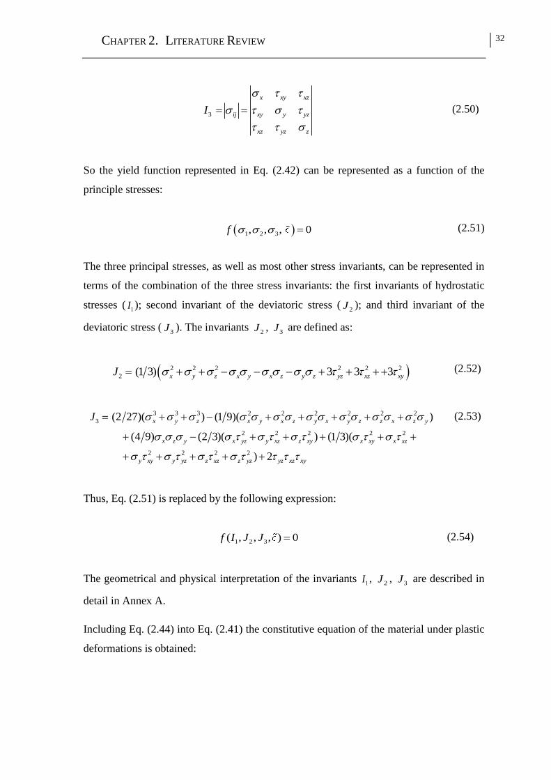
CHAPTER 2. LITERATURE REVIEW 32
3
x xy xz
ij xy y yz
xz yz z
I
(2.50)
So the yield function represented in Eq. (2.42) can be represented as a function of the
principle stresses:
1 2 3, , , 0f (2.51)
The three principal stresses, as well as most other stress invariants, can be represented in
terms of the combination of the three stress invariants: the first invariants of hydrostatic
stresses (1I ); second invariant of the deviatoric stress (
2J ); and third invariant of the
deviatoric stress (3J ). The invariants
2J , 3J are defined as:
2 2 2 2 2 2
2 (1 3) 3 3 3x y z x y x z y z yz xz xyJ
3 3 3 2 2 2 2 2 2
3
2 2 2 2 2
2 2 2 2
(2 27)( ) (1 9)( )
(4 9) (2 3)( ) (1 3)(
) 2
x y z x y x z y x y z z x z y
x z y x yz y xz z xy x xy x xz
y xy y yz z xz z yz yz xz xy
J
(2.52)
(2.53)
Thus, Eq. (2.51) is replaced by the following expression:
1 2 3( , , , ) 0f I J J (2.54)
The geometrical and physical interpretation of the invariants 1I ,
2J , 3J are described in
detail in Annex A.
Including Eq. (2.44) into Eq. (2.41) the constitutive equation of the material under plastic
deformations is obtained:

CHAPTER 2. LITERATURE REVIEW 33
( )e
ij
gD
(2.55)
The system of equations for the plasticity model includes the Eqs. (2.45), (2.54), and
(2.55) that should be solved for set of the unknowns that are components of the stress
tensor, and the plasticity internal variables, and .
2.5 CONCLUSIONS
Based on the literature review presented in this chapter, the following decisions are made
for the development of a new constitutive model described in the next chapters:
The model adopts a multidirectional fixed smeared cracking approach to account
for crack opening and shear sliding process of concrete. It was discussed in this
chapter that the models based on the smeared cracking approach are less precise
on prediction of localization and propagation of the discrete cracks, but they are
more appropriate for simulating relatively large concrete structures, mainly those
with reinforcement that assure the formation of relatively high number of cracks.
Besides, it is of special interest to use the proposed model for simulating
structures made of steel fiber cement based materials. Since this type of materials
assures formation of diffuse crack patterns, due to reinforcing mechanisms of
fibers bridging the cracks, thus a smeared crack model can be practically more
appropriate when compared to a model based on discrete crack approach.
The proposed model simulates the inelastic compressive behaviour of material
between cracks, by a numerical strategy that combines plasticity and damage
theories. As it was argued in literature review, the models based on plasticity or
damage theories alone are not able to describe some important mechanical
behaviour of concrete (see section 2.3). So, in the proposed model, plasticity and
damage theories are being merged in an attempt of constituting reliable
approaches capable of simulating the strength and stiffness degradation and
occurrence of irreversible deformations of concrete in compression.

CHAPTER 2. LITERATURE REVIEW 34
Combination of the plasticity and damage theories is assured by considering that
the plastic flow occurs in undamaged (with respect to compression) material,
together with the strain based damage approach assuming state of damage equally
distributed in all the material directions (isotropic damage). This type of coupling
between the damage and plasticity was noticed robust and numerically efficient by
many authors (as discussed in section 2.3). The isotropic damage approach is
considered for the proposed model because of its convenience and applicability in
structural analysis.

C H A P T E R 3
TWO DIMENSIONAL PLASTIC-DAMAGE
MULTIDIRECTIONAL FIXED SMEARED CRACK
MODEL
3.1 INTRODUCTION
In this chapter the development of an efficient model capable of simulating the
nonlinearities of cement based materials, like concrete, subjected to several loading paths
is presented. For this purpose a brief description of an already existing multidirectional
fixed smeared crack (SC) model is made (Sena-Cruz, 2004; Ventura- Gouveia, 2011).
Then, a plasticity-damage model is proposed to consider the inelastic compressive
deformation of material between the cracks, and its coupling with the SC is described.
The predictive performance of the developed model is validated at the material level by
simulating the stress-strain histories of a single element with one integration point (IP),
loaded under some different scenarios. The model appraisal at the structural level is
assessed in the next chapter.
3.2 MULTIDIRECTIONAL FIXED SMEARED CRACK MODEL (SC MODEL)

CHAPTER 3. TWO DIMENSIONAL PLASTIC-DAMAGE MULTIDIRECTIONAL FIXED
SMEARED CRACK MODEL
36
In the present section the SC model is briefly discussed and its presentation is restricted to
plane stress state and at the domain of an IP. In this approach modelling cracked materials
is based on the decomposition of the total incremental strain vector into an incremental
crack strain vector ( cr ) and an incremental concrete strain vector ( co
), as earlier
discussed in section 2.4.3. For the present stage of the model description, it is assumed
that material between cracks develops linear elastic behaviour, therefore the co is the
incremental elastic strain vector ( co e ). To simulate the plastic response of
material in compression, the co should also include the plastic part of the material
deformation, co e p , which will be discussed in the next section.
The constitutive law for the elastic-cracked material can be, therefore, written as:
( )e cr
D (3.1)
being 1 2 12{ , , } the incremental stress vector induced into the material due
to 1 2 12{ , , } and considering the constitutive matrix of the intact material,
eD .
The cr is obtained from the incremental local crack strain vector, cr
, and the
transformation matrix crT according to Eq. (2.32).
The vector cr includes normal ( cr
n ) and tangential ( cr
t ) crack strain components
of the m cracks that can be formed in an IP (see Eq. (2.33)). The transformation matrix of
generic ith crack, cr
iT , is obtained by having orientation of the ith crack, i , that is the
angle between 1x axis and the vector perpendicular to the ith crack (Sena-Cruz, 2004).
At the crack zone (damage material) of an IP, the opening and sliding process is governed
by the crack constitutive relationship introduced in Eq. (2.35), (i.e. cr cr crD ).
As defined in section 2.4.3, cr is the vector of the incremental crack stress in the crack
coordinate system with the contribution of normal, cr
n , and tangential components,

CHAPTER 3. TWO DIMENSIONAL PLASTIC-DAMAGE MULTIDIRECTIONAL FIXED
SMEARED CRACK MODEL
37
cr
t , of the m cracks that can be formed in an IP (see Eq. (2.36)). Accordingly the
constitutive law of ith generic crack, cr
iD , is given:
0
0
crcr n
i cr
t
DD
D
(3.2)
where cr
nD and cr
tD represent, respectively, the stiffening/softening modulus
corresponding to fracture mode I (normal), and fracture mode II (shear), of the ith crack.
At the IP the equilibrium condition is assured by imposing the Eq. (2.37), (i.e.
cr crT ).
In the course of the implementation of the constitutive model, it is assumed that at a
certain loading step, n, the stress and strain quantities are known, and the local crack
variables are updated as well. At the onset of the next loading step, n+1, Eq. (2.37) must
be accomplished:
1, 1 1
cr cr
nn nT (3.3)
Including Eqs. (3.1), (2.32) and (2.35) into Eq. (3.3), and taking into account that
, 1 , , 1
cr cr cr
n n n and 1 1n n n , yields, after some arrangements, in:
1 1 1 1 1, , 1 1 , 1 0T
cr cr cr cr cr e cr e cr cr
n n n n nn n n n nD T T D T D T
(3.4)
From the load step n to n+1, the the total strain increment (1 n ) is already calculated
by the main FEM iterative solving algorithm. Afterward the Newton-Raphson method is
used to solve the Eq. (3.4), the system of nonlinear equations, where the unknowns are
the components of , 1
cr
n . After obtaining , 1
cr
n , the 1
cr
n and , 1
cr
n are determined
from Eqs. (2.32) and (2.35), respectively, and finally 1 n is calculated from Eq. (3.1).

CHAPTER 3. TWO DIMENSIONAL PLASTIC-DAMAGE MULTIDIRECTIONAL FIXED
SMEARED CRACK MODEL
38
The crack initiation is governed by the Rankine failure criterion that assumes that a crack
occurs when the maximum principal tensile stress in a IP attains the concrete tensile
strength, ctf , under an assumed tolerance. After crack initiation, the relationship between
the normal stress and the normal strain in the crack coordinate system, i.e. cr cr
n n , is
simulated via the trilinear (Sena-Cruz, 2004) or the quadrilinear (Salehian and Barros,
2015) diagrams represented in Fig. 3.1. Normalized strain, i (for trilinear i=1,2; for
quadrilinear i=1,2,3), and stress, i (for trilinear i=1,2; for quadrilinear i=1,2,3),
parameters are used to define the transition points between linear segments, being fG the
fracture energy mode I, while bl is the characteristic length (crack bandwidth) used to
assure that the results of a material nonlinear analysis is not dependent of the refinement
of the finite element mesh.
(a) (b)
Fig. 3.1 – Diagrams for modelling the fracture mode I at the crack coordinate system: (a) trilinear
diagram (Sena-Cruz, 2004), (b) quadrilinear diagram (Salehian and Barros, 2015).
The model considers shear behaviour of the cracked concrete according to two methods:
,sec
cr
nD ,3
cr
nD
,2
cr
nD
2 ctf
1 ctf
,
cr
n u2 ,
cr
n u 1 ,
cr
n u
cr
n
ctf
cr
n
f
b
G
l
,1
cr
nD
cr
n
3 ,
cr
n u
3 ctf,sec
cr
nD,4
cr
nD
,2
cr
nD
2 ctf
1 ctf
,
cr
n u2 ,
cr
n u 1 ,
cr
n u
cr
n
ctf
cr
n
f
b
G
l
,1
cr
nD
,3
cr
nD

CHAPTER 3. TWO DIMENSIONAL PLASTIC-DAMAGE MULTIDIRECTIONAL FIXED
SMEARED CRACK MODEL
39
1) using an incremental crack shear stress shear strain approach based on a shear retention
factor, . According to this approach the fracture mode II modulus, cr
tD , is simulated
as:
1
cr
t cD G
(3.5)
where cG is the concrete elastic shear modulus, while the shear retention factor , , can
be a constant value or, alternatively, as a function of current crack normal strain, cr
n , and
of ultimate crack normal strain, ,
cr
n u , such as:
1
,
1
Pcr
n
cr
n u
(3.6)
being the exponent P1 a parameter that defines the decrease rate of with increasing cr
n
.
2) adopting a cr cr
t t softening law to simulate more correctly the shear stress transfer
during the crack opening process, which allows better predictions in terms of load
carrying capacity, deformability, and crack pattern of RC elements failing in shear
(Ventura-Gouveia, 2011). The adopted shear softening law is represented in Fig. 3.2, and
can be formulated by the following equation (Ventura-Gouveia, 2011):
,1 ,
,
, , , ,
, ,
,
0
0
cr cr cr cr
t t t t p
cr
t pcr cr cr cr cr cr cr
t t p t t p t p t t ucr cr
t u t p
cr cr
t t u
D
(3.7)
where ,
cr
t p is the crack shear strength (shear stress at peak), , , ,1
cr cr cr
t p t p tD is the crack
shear strain at peak, and ,
cr
t u is the ultimate crack shear strain:

CHAPTER 3. TWO DIMENSIONAL PLASTIC-DAMAGE MULTIDIRECTIONAL FIXED
SMEARED CRACK MODEL
40
,
,
,
2 f scr
t u cr
t p b
G
l
(3.8)
being ,f sG the fracture energy corresponding to fracture mode II, and
bl the crack
bandwidth that is assumed to be equal to the one adopted to simulate the fracture mode I.
Since no dedicated research is available on the process of determining the crack
bandwidth parameter that bridges crack shear slide with shear deformation in the smeared
shear crack band, it was decided to adopt the same strategy for the crack bandwidth
regardless the type of fracture process. This decision has, at least, the advantage of
assuring the same results regardless the mesh refinement, which is not assured when
using the concept of shear retention factor in structures failing in shear. The inclination of
the hardening branch of diagram, ,1
cr
tD (see Fig. 3.2), is introduced according to (3.5)
where is set as a constant value in the range 0,1 . More details corresponding to the
crack shear softening diagram can be found elsewhere (Ventura-Gouveia, 2011).
Fig. 3.2 – Diagram for modelling the fracture mode II at the crack
coordinate system (Ventura-Gouveia, 2011).
Fig. 3.3 represents a schematic representation of the crack shear stress-shear strain
diagram for the incremental approach based on shear retention factor (Eq. (3.5) and Eq.
1 - Stiffening
2 - Softening
3 - Unloading
4 - Reloading
5 - Free-sliding
Shear Crack Statuses
t,p
constant shear
retention factor
Dt,3-4
Gf,s
lb
cr
cr
t,max cr
cr
t,u cr
t,max cr
t,p
t,max- cr
- cr
t,u- cr
t,max- cr
t,p
t,p- cr
cr
2
1
3
4
5
1
2
43
5
crDt,1
cr
Dt,2
cr
t
t

CHAPTER 3. TWO DIMENSIONAL PLASTIC-DAMAGE MULTIDIRECTIONAL FIXED
SMEARED CRACK MODEL
41
(3.6)). It is verified that with the increase of cr
t the crack shear modulus, cr
tD , decreases
but the crack shear stress, cr
t , increases up to attain a maximum that depends on the
parameters considered for the Eq. (3.6). This value can be much higher than the concrete
shear strength according to available experimental data and design guidelines.
Fig. 3.3 – Relation between crack shear stress and crack shear strain for the
incremental approach based on a shear retention factor (Barros et al., 2011).
For RC elements failing in bending the maximum value of cr
t is relatively small,
therefore simulating shear stress degradation with the evolution of cr
t has not relevant
impact of the predictive performance of the simulations. However, in RC structures
failing in shear, the adoption of a constitutive law capable of simulating the crack shear
stress degradation, as the one adopted in the present work, is fundamental for the
predictive performance. The computing time consuming and the convergence stability of
the incremental and iterative procedure of the model when adopting softening diagrams
for simulating all the fracture processes are, however, increased, therefore shear softening
approach is only recommended when shear is the governing failure mode.
3.3 PLASTIC-DAMAGE MULTIDIRECTIONAL FIXED SMEARED CRACK
MODEL (PDSC MODEL)
The SC model described in the section 3.2 is now extended in order to simulate the
inelastic behaviour of cement based materials in a compression-compression and
,5
cr
tD
,3
cr
tD
,2
cr
tD
cr
t
cr
t
,1
cr
tD
,4
cr
tD

CHAPTER 3. TWO DIMENSIONAL PLASTIC-DAMAGE MULTIDIRECTIONAL FIXED
SMEARED CRACK MODEL
42
compression-tension stress fields. For this purpose a plastic-damage approach is coupled
with the SC model, deriving a model herein designated as plastic-damage multidirectional
fixed smeared crack (PDSC) model, which is capable of simulating the nonlinear
behaviour of cement based materials due to both cracking and inelastic deformation in
compression.
3.3.1 Damage concept in the context of plastic-damage model
To demonstrate the process of damage evolution in compression when an isotropic
damage model is applied to simulate strength and stiffness degradation in compression, a
simple bar loaded in compression is presented. This problem is similar to the case of the
bar under tension proposed by Kachonov (1958). Consider a bar made by cement based
materials and exposed to a certain level of damage due to uniaxial compressive force, N ,
as illustrated in Fig. 3.4a (Abu Al-Rub and Kim, 2010). The total cross-sectional area of
the bar in damaged, nominal, status is denoted by A , then the stress developed on this
area is defined as N A , herein designated as nominal stress. Due to the thermo-
hygrometric effects during the curing process of cement based materials, voids and
micro-cracks are formed even before these materials have been loaded by external loads
(Pereira, 2012). However, the impact of these “defects” in terms of stiffness and strength
of the material can be neglected, and the degeneration of the micro- into meso- and macro
cracks is generally a gradual damage process depending on the evolution of the external
loading conditions. Let’s assume the variable DA represents the area corresponding to
these defects (meso- and macro cracks) (Fig. 3.4b). According to the principle of
isotropic damage approach, a scalar measure, cd , is defined to represent this damage
level in total cross-sectional area ( A ), such that:
Dc
Ad
A (3.9)
that can take values from 0 to 1. The state cd =0 implies the area of A is intact, while
cd =1 denotes the area of A is completely damaged.

CHAPTER 3. TWO DIMENSIONAL PLASTIC-DAMAGE MULTIDIRECTIONAL FIXED
SMEARED CRACK MODEL
43
Fig. 3.4 – One dimensional representation of the effective and nominal
stresses (Abu Al-Rub and Kim, 2010).
A fictitious undamaged, effective, area of A , is defined by removing all the damage
regions from the area of A ( 1D cA A A d A ), then the uniaxial stress developed
on the area A , N A , is denoted as effective stress (Fig. 3.4c). Since the applied
force on both damaged and undamaged areas is N , then the following relation holds
between the uniaxial stress at damaged (nominal), , and undamaged (effective), ,
configurations:
1 cd (3.10)
By extending this concept for a multidimensional stress field, the relation between the
nominal stress vector ( ), and the effective stress vector ( ) for isotropic damage
models can be expressed as:
1 cd (3.11)
The present study adopts a stress based plasticity model formulated in effective stress
space in combination with an isotropic damage model. The resultant plastic-damage
approach is meant to utilize for modelling inelastic deformation of material under
compression.
(a) the bar under compression (c) Effective (undamaded)
configuration
N
A
NA
N
A
A
Remove the cracks
DA (Area of the cracks)
N
(b) Nominal (damaded)
configuration

CHAPTER 3. TWO DIMENSIONAL PLASTIC-DAMAGE MULTIDIRECTIONAL FIXED
SMEARED CRACK MODEL
44
Fig. 3.5 – Schematic representation of damage evolution in the proposed model.
An important assumption of the proposed plastic-damage model is to define the stage that
damage initiation takes place. In this study the damage threshold was assumed based on
the phenomenological interpretation of the behaviour of current concrete under
compressive loading. In section 2.2.1 the three distinct consecutive stages (stage I, stage
II, and stage III) of cracking that can be identified in concrete under uniaxial compressive
load were introduced. In this study damage initiation is assumed to be related to
development of the major cracks formed after the peak load (i.e. stage III). Then
evolution of the damage through the stage II is considered to be null ( cd =0), and
nonlinear behaviour of the current concrete in this stage is reproduced by only a plasticity
model. At the stage III the plasticity model is responsible for simulating irreversible
plastic deformation and inelastic volumetric expansion of the material whereas the
isotropic damage model deals with strength and stiffness degradation of the material due
to formation of the major cracks. Fig. 3.5 demonstrates the schematic representation of
the damage evolution at the proposed plastic-damage model for the three stages of
cracking in uniaxial compression.
It is noted the statement of “damage” in the text intends to simulate the inelastic
behaviour of concrete in compression by using a plastic-damage model, while cracking
formation and propagation is simulated by a SC model. Therefore, if concrete is cracked
and concrete between cracks experience inelastic deformation in compression, both
models are coupled.
1-d
c
Stag
e
Stage
0
1.0
Compressive deformation

CHAPTER 3. TWO DIMENSIONAL PLASTIC-DAMAGE MULTIDIRECTIONAL FIXED
SMEARED CRACK MODEL
45
3.3.2 Constitutive relationship for PDSC model
For modelling of a cracked member with material between cracks in compression, the
term co is further decomposed into its elastic, e
, and plastic parts, p , (
co e p ), thereby the incremental constitutive relation for the PDSC model is
given by:
( )e p cr
D (3.12)
where the incremental crack strain vector, cr , is evaluated by the SC model described
in section 3.2. A stress based plasticity model formulated in effective stress space, i.e.
without considering damage, is responsible for the evaluation of p . The plasticity
model assumes that plastic flow occurs on the undamaged material between the damaged
regions formed during the strain softening compression stage of the material. Then the
effective stress state obtained according to Eq. (3.12) needs to be mapped into nominal
stress space according to the principle of CDM. This mapping process should distinguish
the tensile from the compressive stress components, since the damage is only applied to
these last ones. Ortiz (1985) proposed the split of the effective stress vector, , into
positive (tensile) and negative (compressive) components to adopt different scalar
damage variables for tension and compression. Such operation is given by:
,i ii
i
P P
(3.13)
where
and
are the positive and the negative parts of the effective stress vector,
respectively, and i is the ith
principal stress extracted from vector , and iP is the
normalized eigenvector associated with the ith
principal stress ( i ). The symbol .
denotes Macaulay bracket function operating as ( ) 2x x x .

CHAPTER 3. TWO DIMENSIONAL PLASTIC-DAMAGE MULTIDIRECTIONAL FIXED
SMEARED CRACK MODEL
46
The compressive damage scalar, cd , must affect only the negative part of the effective
stress vector, i.e. , therefore a similar approach to Eq. (3.11) gives the nominal stress
vector, such as:
(1 )cd
(3.14)
3.3.3 – Plasticity model in effective stress space
The plastic strain vector, p , is evaluated by a time-independent plasticity model that is
defined by four entities: yield function (yield surface); flow rule; evolution law for the
hardening variable; and condition for defining loading-unloading process. In this study
the yield function, f, was derived from the five-parameter Willam and Warnke (W-W)
failure criterion (Willam and Warnke, 1974) (the details of this process are in the Annex
B), which shows a good ability to represent the experimental results of cement based
materials (Willam and Warnke, 1974; Swaddiwudhipong and Seow, 2006), and also
satisfies all the requirements of being smooth, convex, pressure dependent, and curved in
the meridian plane. The equation of this yield function is:
1/2
12 2
2 2; ( ) ( ) ( ) 0
3c c c c c c
I b af J J
c cc
(3.15)
where 1I is the first invariant of the effective stress tensor, 2J is the second invariant of
the deviatoric effective stress tensor (see Eq. (2.48) and Eq. (2.52), respectively). The
variables a, b and c are the scalars used to interpolate the current yield meridian between
the tensile and compressive meridians, as described in detail in the Annex B.
The term ( )c c , which appears in Eq. (3.15), is the hardening function depending on the
hardening parameter (c). The hardening parameter is a scalar measure used to
characterize the plastic state of the material under compressive stress field. Therefore c
is an indicator of the degree of inelastic deformation the material has experienced during
the loading history. The evolution of the yield surface during the plastic flow is governed

CHAPTER 3. TWO DIMENSIONAL PLASTIC-DAMAGE MULTIDIRECTIONAL FIXED
SMEARED CRACK MODEL
47
by c. As long as
c is null, no inelastic deformation occurred, and ( ; ( 0)) 0 c cf
corresponds to the initial yield surface.
When the effective stress state reaches to the yield surface at generic stage (i) of yielding
process, 0if , plastic strains are developed, being its increment evaluated by a flow
rule:
p g
(3.16)
where g is a scalar function, called plastic potential function, and is the non-negative
plastic multiplier. In the present version of the model, g f was assumed (Dunne and
Petrinic, 2005).
The state of hardening parameter, c , during the plastic flow is changed according to the
following evolution law (Ristinmaa et al., 2007):
c
c
f
(3.17)
The yield function ( f ) and plastic multiplier ( ) at any stage of loading and unloading
paths are constrained to follows Kuhn-Tucker conditions:
0, ( , ) 0, ( , ) 0c cf f (3.18)
3.3.3.1 Hardening law
Compressive behaviour of the material in effective stress space is governed by the
uniaxial hardening law of c c (Fig. 3.6a). The term
c is the uniaxial compressive
stress in effective stress space, and the hardening parameter ( c ) is an equivalent plastic
strain measure that is proportional to the plastic strain (p
) developed in the material.

CHAPTER 3. TWO DIMENSIONAL PLASTIC-DAMAGE MULTIDIRECTIONAL FIXED
SMEARED CRACK MODEL
48
Hardening parameter corresponding to total axial strain at compression peak stress (1c)
is obtained such that:
1 1c c cf E (3.19)
being 1c the total strain at compression peak stress, and cf the compressive strength.
In this study it is assumed that the compressive damage, cd , is initiated at the plastic
deformation corresponding to 1c, i.e. if
1c c, then
cd =0 (Fig. 3.6b). According to this
assumption, the effective and nominal responses are identical for the domain of 1c c
(Eq. (3.15) assuming cd =0). Then c c for the domain of
1c c can be directly
obtained by experimental uniaxial stress-strain curves, which are in the nominal stress
space, such relation was adopted according to the following equation:
1 2c c cE E (3.20)
where:
2 2
0 0 0 1 1( 1) ( ) 2 ( )c c c c cf f E f E
1/22
1( ) ( (2 ))c c cE f E E
(3.21)
(3.22)
where 0cf is the uniaxial compressive strength at plastic threshold, i.e.
0 0( 0) c c c cf f , and 0 is a material constant to define the beginning of the
nonlinear behaviour in uniaxial compressive stress-strain test.
For 1c c, the damage takes place ( 0cd ), then the effective stresses cannot be
determined by direct identifications from relevant uniaxial compressive stress-strain tests
(Gernay et al., 2013; Abu Al-Rub and Kim, 2010). For this domain (1c c) and in order
to reduce the number of parameters required in the plasticity model, a perfectly-plastic
behaviour is assumed for the c c law, with an effective stress capacity equal to the

CHAPTER 3. TWO DIMENSIONAL PLASTIC-DAMAGE MULTIDIRECTIONAL FIXED
SMEARED CRACK MODEL
49
compressive strength of the material, ( ) c c cf . Fig. 3.6a represents the above
described hardening law ( c c ). In Annex C, the adopted c c law for the domain
1c c is replaced by a more elaborated equation, and the resultant response of the
proposed model in cyclic uniaxial compressive test is discussed.
(a) (b)
(c)
Fig. 3.6 – Diagrams for modelling the concrete compression behaviour: (a) the c c relation
used in the plasticity model; (b) the (1 )c dd relation adopted in the isotropic damage
model; (c) the (1 )c c cd diagram for compression with indication of the compressive
fracture energy, ,f cG .
3.3.3.2 System of nonlinear equations
Assuming the material is in uncracked stage, or eventually the former active cracks are
completely closed, then the incremental crack strain is null, 0cr
, and the
constitutive law of PDSC model, Eq. (3.12), is reduced to:
c
cf
1c,c u
c
0 0c cf f
,( . . )c c ui e 0d
d
1( . . )c ci e , 1d c u c
1.0
(1 )cd
0 0c cf f
cf
1c
(1 )c cd
,f c
c
G
l
c
,c u

CHAPTER 3. TWO DIMENSIONAL PLASTIC-DAMAGE MULTIDIRECTIONAL FIXED
SMEARED CRACK MODEL
50
( )e p
D (3.23)
It is assumed that at a certain loading step of the incremental/iterative Newton-Raphson
algorithm generally used for solving the equilibrium of the structure, n, the stress and
strain quantities and the local variables of the plasticity (n and
,c n) are known at all
IPs. At the next loading step (n+1) the increment of total strain vector (1n ) is
calculated by the main FEM iterative solving algorithm, and the problem is to update the
effective stress vector (1n ), the increment of plastic strain vector (
1
p
n ) and the local
variables of the plasticity (1n and
, 1c n), in a way that is consistent with the
constitutive law.
A mathematical basis scheme called return-mapping algorithm (Simo and Hughes, 1998)
is used to calculate these unknowns within a generic loading step (n+1). The return-
mapping algorithm is strain driven and basically consists of two steps: calculation of the
elastic trial stress, elastic-predictor step, and mapping back to the proper yield surface
using a local iterative process, plastic-corrector step. In the first approximation (elastic-
predictor step), the effective stress vector (1
trial
n ) is calculated assuming null value for the
plastic strain increment (the total strain increment is assumed to be elastic, 1 1
e
n n
). In this step null plastic multiplier is assumed (1 0n ) and hardening parameter has
the value corresponding to the previous loading step (n). The conditions at the elastic-
predictor step can be written as:
,
1 1
,
1 1 11
1 1
,
1 , 1 ,
, 1 ,
0; 0
( )
;
p trial trial
n n
p trialtrial e e
n n nn
trial trial
n n n
p trial p trial
n n c n c n
trial
c n c n
D D
(3.24)
Substitution of Eq. (3.24) into Eq. (3.15), gives the yield surface in trial state as:

CHAPTER 3. TWO DIMENSIONAL PLASTIC-DAMAGE MULTIDIRECTIONAL FIXED
SMEARED CRACK MODEL
51
1 1 1 , 1( , )trial trial trial trial
n n n c nf f (3.25)
Then behaviour of the material remains elastic if:
1 1 , 1( , ) 0trial trial trial
n n c nf (3.26)
In this case (1 0trial
nf ), it can be seen that the Kuhn-Tucker conditions are satisfied (
1 1 , 1( , ) 0trial trial trial
n n c nf and 1 0trial
n ), implying that the trial state of stress (1
trial
n ) is
acceptable. The updated variables at the load step n+1 are given as:
11 1 , 1 ,; ;p ptrial
n nn n c n c n (3.27)
Otherwise, if 1 1 , 1( , ) 0trial trial trial
n n c nf , the material enters into elasto-plastic behaviour
(plastic flow occurs). In this case (1 0trial
nf ), the effective stress vector, at the load step
n+1, should be corrected by applying a plastic-corrector step such that:
1 11
1 1 11
( )
( )
pe
n nn n
p pe e trial e
n n nn n
elastic predictor Plastic corrector
D
D D D
(3.28)
Including Eq. (3.16) in Eq. (3.38), yields:
1 1 1 1 1( )trial e
n n n n n
elastic predictor Plastic corrector
D f (3.29)
The hardening variable at the loading step n+1 should be updated according to the
following equations:
1, 1 1
, 1
, 1 , , 1
nc n n
c n
c n c n c n
f
(3.30)
(3.31)

CHAPTER 3. TWO DIMENSIONAL PLASTIC-DAMAGE MULTIDIRECTIONAL FIXED
SMEARED CRACK MODEL
52
The system of equations for the proposed plasticity model includes the Eqs. (3.15),
(3.29), (3.31) which can be rewritten in the form:
11
1, 1 1 1 1
1
12, 1 , 1 1
, 1
3, 1 1 1 , 1
( ) 0
0
, 0
e trial nn n n n
n
nn c n c n
c n
n n n c n
ff D
ff
f f
(3.32a)
(3.32b)
(3.32c)
The unknowns of the system of equations are the components of effective stress vector,
1n , and the plasticity internal variables,
1n and , 1c n
. An iterative local Newton-
Raphson method is used to solve this system of equations, according to the following
equation:
( 1) ( )
1 1, 1
( ) ( 1) ( )
1 , 1 2, 1
( 1) ( )
1 3, 1
k k
n n
k k k
n c n n
k k
n n
d r
J d r
d r
(3.33)
Within this procedure the objective is to minimize the residues vector,
( ) ( ) ( )
1, 1 2, 1 3, 1
Tk k k
n n nr r r , to be less than an assumed tolerance. The variable k
denotes the iteration required to minimize the residues vector. For this system of
equations the residues ( )
1, 1
k
nr , ( )
2, 1
k
nr , ( )
3, 1
k
nr are given as:
( )1
( ) ( ) ( ) 11, 1 1 1 1 ( )
1
( )( ) ( ) ( ) 1
2, 1 , 1 , 1 ( )
, 1
( ) ( ) ( ) ( )
3, 1 1 1 , 1
( )
,
kk e k trial k nn n n n k
n
kk k k nn c n c n n k
c n
k k k k
n n n c n
fr D
fr
r f
(3.34)

CHAPTER 3. TWO DIMENSIONAL PLASTIC-DAMAGE MULTIDIRECTIONAL FIXED
SMEARED CRACK MODEL
53
The Jacobian matrix (( )
1
k
nJ ) used in the iterative local Newton-Raphson method is given:
( )
1, 1 1, 1 1, 1
1 , 1 1
2, 1 2, 1 2, 1( )
1
1 , 1 1
3, 1 3, 1 3, 1
1 , 1 1
k
n n n
n c n n
n n nk
n
n c n n
n n n
n c n n
f f f
f f fJ
f f f
(3.35)
where the components of the Jacobian matrix are as follows:
211, 1 1
1 2
1 1
21, 1 , 11
1
, 1 1 , 1 , 1
1, 1 1
1 1
n e nn
n n
n c nnn
c n n c n c n
n n
n n
f fD
f f
f f
(3.36)
22, 1 1
1
1 , 1 1
22, 1 , 11
1 2
, 1 , 1, 1
2, 1 1
1 , 1
1
n nn
n c n n
n c nnn
c n c nc n
n n
n c n
f f
f f
f f
(3.37)
3, 1 1
1 1
3, 1 , 11
, 1 , 1 , 1
3, 1
1
0
n n
n n
n c nn
c n c n c n
n
n
f f
f f
f
(3.38)

CHAPTER 3. TWO DIMENSIONAL PLASTIC-DAMAGE MULTIDIRECTIONAL FIXED
SMEARED CRACK MODEL
54
The implementation of Eq. (3.35) requires other derivatives which are exposed in details
in Annex D. These derivatives are: first and second order derivatives of the yield function
respect to components of the effective stress vector (i.e. f , 2 2( )f ); first and
second order derivatives of the yield function respect to the hardening function (cf ,
2 2( )cf ); the second order derivative of the yield function respect to the stress, and
respect to the hardening function ( 2 ( )cf ).
Once the convergence is obtained through the certain number of iteration (k), i.e. the
residues ( )
1, 1
k
nr , ( )
2, 1
k
nr , ( )
3, 1
k
nr are less than an assumed tolerance, the unknowns can be
obtained by summation of the increments calculated in each iteration (i=1 to k):
( ) ( )
1 1
1
( ) ( )
, 1 , , 1
1
( ) ( )
1 1
1
kk i
n n n
i
kk i
c n c n c n
i
kk i
n n
i
d
d
d
(3.39)
3.3.4 – Coupling the plasticity and the SC models
In this section the plasticity model, formulated in effective stress space, and the
multidirectional smeared crack (SC) model are combined within an integrated approach
in order to be capable of evaluating cr and p
simultaneously at a generic IP. For a
loading path the computation of the unknowns, which are the effective stress state and the
local variables of the plasticity and cracking models, follows an iterative process similar
to the return-mapping algorithm indicated in 3.3.3.2.
In the first approximation of the unknowns (elastic-predictor step), values of effective
stress vector, i.e. trial stress (1
trial
n ), and incremental crack strain vector ( ,
1
cr trial
n ), and
the local crack variables are calculated by only the SC model assuming the elastic
behaviour for the material under compressive deformations. In this step null plastic
multiplier is assumed (1 0trial
n ) and hardening parameter has the value corresponding

CHAPTER 3. TWO DIMENSIONAL PLASTIC-DAMAGE MULTIDIRECTIONAL FIXED
SMEARED CRACK MODEL
55
to the previous loading step (n). The conditions at the elastic-predictor step can be written
as:
, ,
1 11
,
1 11
1 1
, 1 , , 1 ,
0 ; 0 ;
( )
;
p trial p trial ptrial
n n nn
cr trialtrial e
n nn
trial trial
n n n
trial trial
c n c n c n c n
D
(3.40)
The value of yield function at the trial state, 1 1 , 1( , )trial trial trial
n n c nf , is calculated next.
Behaviour of the material remains elastic-cracked if 1 0trial
nf , while for 1 0trial
nf ,
material enters into elasto-plastic-cracked behaviours and the state of effective stress
needs to be corrected by determining the plastic part of strain increment (1
p
n ), (plastic-
corrector step).
As indicated in section 3.1, the equilibrium condition for a cracked IP is assured when:
Introducing 1 1n n n into Eq. (3.41), yields after some arrangements in:
1 1, , 1 11, 1 0cr cr cr cr
n nn n nnf D T (3.42)
The system of equations proposed for the plasticity model (in section 3.3.3.2) needs also
to be modified to include the deformational contribution of the sets of active smeared
cracks ( cr ). By considering
1 1n n n and introducing Eqs. (2.32) and (3.16)
into Eq. (3.12), yields after some arrangements in:
11 1 , 12, 1 1
1
( ) 0T
e cr cr e
nn n n nn n
n
ff D T D
(3.43)
1 1, , 1 1
cr cr cr cr
n nn n n nD T (3.41)

CHAPTER 3. TWO DIMENSIONAL PLASTIC-DAMAGE MULTIDIRECTIONAL FIXED
SMEARED CRACK MODEL
56
The equations describing the yield function (Eq. (3.32c)) and the evolution law for
hardening variable (Eq. (3.32b)), still hold in the form deduced in section 3.3.3.2, since
these equations are not affected by cr . In this section these two equations are
designated as the followings:
13, 1 , 1 1
, 1
0nn c n c n
c n
ff
4, 1 1 1 , 1, 0n n n c nf f
(3.44)
(3.45)
The system of equations includes the Eqs. (3.42)-(3.45) which should be solved for set of
the unknowns, namely, the effective stress vector, 1n , the incremental local crack strain
vector, , 1
cr
n , the plastic multiplier, 1n , and the hardening parameter,
, 1c n, all of
them at the n+1 loading increment. An iterative local Newton-Raphson method is used to
solve this system of equations, according to the following equation:
( ),( 1)
1, 1, 1
( )( 1)2, 1( ) 1
1 ( )( 1)3, 1, 1
( )( 1)4, 11
kcr k
nn
kknk n
n kknc n
kknn
rd
rdJ
rd
rd
(3.46)
where the residues are:
,( ) ,( ) ,( ) ,( )( )
1 1, , 1 11, 1
( )1 ( ) ,( ) ,( )( ) ( ) ( ) 1
11 , 12, 1 1 1 ( )
1
( )( ) ( ) ( ) 1
3, 1 , 1 , 1
cr k cr k cr k cr kk
n nn n nn
kT
k cr k cr kk e k e k nnn n nn n n k
n
kk k k nn c n c n n
r D T
fr D D T
fr
( )
, 1
( ) ( ) ( ) ( )
4, 1 1 1 , 1,
k
c n
k k k k
n n n c nr f
(3.47a)
(3.47b)
(3.47c)
(3.47d)
The Jacobian matrix (( )
1
k
nJ ) used in the iterative local Newton-Raphson method is given:

CHAPTER 3. TWO DIMENSIONAL PLASTIC-DAMAGE MULTIDIRECTIONAL FIXED
SMEARED CRACK MODEL
57
1, 1 1, 1 1, 1 1, 1
1 , 1 1, 1
2, 1 2, 1 2, 1 2, 1
1 , 1 1, 1( )
1
3, 1 3, 1 3, 1 3, 1
1 , 1 1, 1
4, 1 4, 1 4
1, 1
n n n n
cr
n c n nn
n n n n
cr
n c n nnk
n
n n n n
cr
n c n nn
n n
cr
nn
f f f f
f f f f
Jf f f f
f f f
( )
, 1 4, 1
, 1 1
k
n n
c n n
f
(3.48)
where the components of the Jacobian matrix, Eq. (3.52), are as follows:
1, 1
1
, 1
1, 1
1
1
1, 1
, 1
1, 1
1
0
0
n cr
ncr
n
n cr
n
n
n
c n
n
n
fD
fT
f
f
(3.49)
2, 1
1
, 1
212, 1 1
1 2
1 1
22, 1 , 1 1
1
, 1 , 1 , 1 1
2, 1 1
1 1
Tn cr
ncr
n
n e nn
n n
n c n nn
c n c n c n n
n n
n n
fT
f fD
f f
f f
(3.50)

CHAPTER 3. TWO DIMENSIONAL PLASTIC-DAMAGE MULTIDIRECTIONAL FIXED
SMEARED CRACK MODEL
58
3, 1
, 1
23, 1 1
1
1 1 , 1
23, 1 , 1 1
1 2
, 1 , 1, 1
3, 1 1
1 , 1
0
1
n
cr
n
n nn
n n c n
n c n nn
c n c nc n
n n
n c n
f
f f
f f
f f
(3.51)
4, 1
, 1
4, 1 1
1 1
4, 1 , 1 1
, 1 , 1 , 1
4, 1
1
0
0
n
cr
n
n n
n n
n c n n
c n c n c n
n
n
f
f f
f f
f
(3.52)
Finally, once the convergence is obtained, i.e. the residues of the system of equations are
less than an assumed tolerance, the unknowns can be obtained by summation of the
increments calculated in each iteration (i=1 to k), such as:
( ) ( )
1 1
1
( ) ( )
, 1 , , 1
1
( ) ( )
1 1
1
,( ) ,( )
, 1 , 1
1
kk i
n n n
i
kk i
c n c n c n
i
kk i
n n
i
kcr k cr i
n n
i
d
d
d
d
(3.53)

CHAPTER 3. TWO DIMENSIONAL PLASTIC-DAMAGE MULTIDIRECTIONAL FIXED
SMEARED CRACK MODEL
59
3.3.5 – Isotropic damage law
The stress vector (1n ) obtained by solving the system of equations presented in the
sections 3.3.3.2 and 3.3.4 is in the effective stress space, and must be transferred to the
nominal stress space (1n ). For the damage models based on the isotropic damage
mechanics, the evaluation of the nominal stress is performed by a damage-corrector step
(Eq. (3.11)) without an iterative calculation process. The present model adopts a damage-
corrector process according to the Eq. (3.14), which considers the compressive damage
scalar (cd ) only for negative (compressive) part of effective stress vector. The evaluation
of the compressive damage scalar (cd ) during loading history is obtained according to
the approach proposed by Gernay et al. (2013):
( ) 1 exp( )c d c dd a (3.54)
where d
is a scalar parameter known as damage internal variable.
Accordingly, the damage internal variable, d
, can be evaluated as a function of the
plasticity hardening variable, c, which is available at the end of plasticity analysis. As
indicated in section 3.3.3.1, damage initiates at the plastic deformation corresponding to
1c, then the damage internal variable,
d, can be defined as:
1
1 1
0 c c
d
c c c c
if
if
(3.55)
The non-dimensional parameter ca indicates the rate of damage with the variation of
d,
obtained from:
, 12.3 / ( )c c u ca (3.56)

CHAPTER 3. TWO DIMENSIONAL PLASTIC-DAMAGE MULTIDIRECTIONAL FIXED
SMEARED CRACK MODEL
60
being ,c u
the ultimate hardening parameter that is related to the compressive fracture
energy, ,f cG , the characteristic length for compression,
cl , the compressive strength, cf ,
and 1c according to the following equation:
,
, 1
3.1 11
48
f c
c u c
c c
G
l f (3.57)
The characteristic lengths in tension (crack bandwidth) and compression (cl ) are usually
considered the same (Feenstra, 1993; Lee and Fenves, 2001; Gernay et al., 2013), then in
the present approach c bl l was assumed. The parameters E,
0 , cf ,
1c , ,f cG , which
simulate the response of the material under compression, can be obtained by executing
uniaxial compression tests carried out in high stiff rigs, under displacement control, with
specimens of slenderness capable of assuring a central zone considered in uniaxial stress
field (it is assumed the same E in compression and tension). The instruction to derive the
parameter ,f cG , from the uniaxial compressive tests, independent of geometry of
specimens is represented in Annex E, but the detailed exposition can be found elsewhere
(Jansen and Shah, 1997; Vasconcelos et al., 2009).
3.4 SIMULATION AT THE MATERIAL LEVEL
The stress-strain histories at the material (single element with one IP), loaded on some
different scenarios are simulated by the proposed PDSC model. The loading procedure of
the tests consists of imposing prescribed displacement increments and the crack
bandwidth (bl ) was assumed equal to 100 mm. Since the concrete properties in each test
were different, the corresponding values are indicated in the caption of the figures.
- Monotonic and cyclic uniaxial compressive tests (Fig. 3.7 and Fig. 3.8): A
monotonic uniaxial compressive test of Kupfer et al. (1969), and a cyclic uniaxial
compressive test of Karsan and Jirsa (1969) are simulated, and the predictive
performance of the proposed model is appraised by comparing the numerical and
experimental results. Fig. 3.7 shows that the hardening and softening stress-strain
branches registered experimentally by Kupfer et al. (1969) are properly fitted by

CHAPTER 3. TWO DIMENSIONAL PLASTIC-DAMAGE MULTIDIRECTIONAL FIXED
SMEARED CRACK MODEL
61
the nominal response of the proposed model. For comparison, Fig. 3.7 also
represents the response of the model in effective stress space. As can be seen the
stress-strain response in both effective and nominal stress spaces are identical for
the domain before attaining the peak (1c c ), whereas for higher deformations (
1c c ) the two responses starts diverging because of the damage initiation
process ( 0cd ). Under the cyclic uniaxial compression the model (nominal stress
response) accurately simulate the stress-strain envelope response registered
experimentally, but overestimates the plastic deformation of the material when
unloading occurs (Fig. 3.8), since the assumption of perfect-plastic behaviour (
( )c c cf ) for the post peak stage (domain 1c c ) of the
c c law is a
simplified approach to reduce the number of parameters required in the plasticity
model.
Fig. 3.7 – Experimental (Kupfer et al., 1969) vs. predicted stress-strain response of
concrete under monotonic uniaxial compressive test: (Values for the parameters of the
constitutive model: poison’s ratio, =0.2; young’s modulus, E=27 GPa; compressive
strength, cf =32 MPa; strain at compression peak stress
1c =0.0023; parameter to define
elastic limit state 0 =0.3; compressive fracture energy,
,f cG =15.1 N/mm).
In Annex D the adopted c c law for the domain
1c c is replaced by a more
elaborated equation which gives better approximation in simulation of the
-0.012-0.01-0.008-0.006-0.004-0.00200.0020.0040
5
10
15
20
25
30
35
40
Axial strain
PDSC model (nominal stress space)
PDSC model (effective stress space)
Experimental results
(MPa)
(,
)
X1
X2

CHAPTER 3. TWO DIMENSIONAL PLASTIC-DAMAGE MULTIDIRECTIONAL FIXED
SMEARED CRACK MODEL
62
unloading phase. Another alternative to better predict the residual strain in
unloading phases is to follow a more sophisticated diagram, like the one proposed
by Barros et al. (2008) but this approach it too demanding in terms of computer
time consuming when integrated in a PDSC model, and when the final goal is
using this model for the analysis of structures of relatively large dimensions.
Fig. 3.8 – Experimental (Karsan and Jirsa, 1969) vs. predicted stress-strain response of
concrete under cyclic uniaxial compressive test: (Values for the parameters of the constitutive
model: =0.2; E=27 GPa; 0 =0.3;
1c =0.0017; cf =28 MPa;
,f cG =11.5 N/mm).
- Simulation of closing a crack developed in one direction, by imposing
compressive load in the orthogonal direction (Fig. 3.9): The element is initially
subjected to the uniaxial tension in the direction of X1 (Step 1). Then a crack is
formed with the orientation of 0º , and further propagated up to a stage that
the crack does not be able to transfer more tensile stresses (fully opened crack
status). At this stage the displacement in the direction of X1 is fixed (Step 2), and
the element is loaded by compressive displacements in the X2 direction up to end
of the analysis (Step 3).
Due to applied compressive displacements, uniaxial compressive stresses are
induced in the material in the X2 direction. Consequently, expansion of the
material in the X1 direction imposes the crack be gradually closing. When the
0 0.001 0.002 0.003 0.004 0.005 0.006 0.0070
5
10
15
20
25
30
35Experimental results
PDSC model (nominal stress space)
PDSC model (effective stress space)
(-1)
(MP
a)
(1-dC)E
E

CHAPTER 3. TWO DIMENSIONAL PLASTIC-DAMAGE MULTIDIRECTIONAL FIXED
SMEARED CRACK MODEL
63
material is in the compression softening phase, in X2 direction, the crack will be
completely closed. When the crack closes, the state of stress is changed to biaxial
compression, and a second hardening-softening response is reproduced
corresponding to the appropriate biaxial state of stress. The above-described
loading path was successfully simulated by the proposed model, and the
prediction agrees well with the solution of Cervenka and Papanikolaou (2008).
Fig. 3.9 – Prediction of the PDSC model for closing a crack developed in one direction,
by imposing compressive load in the orthogonal direction (Values for the parameters of
the constitutive model: =0.2; E=36 GPa; cf =30 MPa;
,f cG =30 N/mm; 1c =0.0022;
0 =0.3; ctf =2.45 MPa;
I
fG =0.05 N/mm; 1 =0.2;
1 =0.7; 2 =0.75;
2 =0.2.
3.5 CONCLUSIONS
This Chapter describes a two dimensional (plane stress) plastic-damage multidirectional
fixed smeared cracking (PDSC) model to simulate the failure process of concrete and
reinforced concrete (RC) structures subjected to different loading paths. The model
proposes a unified approach combining a multidirectional fixed smeared crack model to
simulate the crack initiation and propagation with a plastic-damage model to account for
the inelastic compressive behaviour of concrete between cracks. The smeared crack model
-0.01-0.008-0.006-0.004-0.00200.002
-35
-30
-25
-20
-15
-10
-5
0
5
Cervenka and Papanikolaou (2008)
PDSC model
Str
ess
(MP
a)
Strain (-)
Crack is closed
Compressive strength fc
4
2
23
5
3
Second hardening-softening branches
)(
Biaxial compressive strength
5
4
1
1 First hardening-softening branches
Step3
Step2
closed crack
X2
X1
fully open crack
Step1

CHAPTER 3. TWO DIMENSIONAL PLASTIC-DAMAGE MULTIDIRECTIONAL FIXED
SMEARED CRACK MODEL
64
considers the possibility of forming several cracks in the same integration point during the
cracking process. The plasticity part accounts for the development of irreversible strains
and volumetric strain in compression, whereas the strain softening and stiffness
degradation of the material under compression are controlled by an isotropic strain base
damage model. The model appraisal is performed by simulating several tests at the
material level (single element with one IP). Monotonic and cyclic uniaxial compressive
tests were simulated at first, followed by a sophisticated biaxial tension-compression
numerical test which is intended to demonstrate the interaction between cracking and
plasticity-damage parts of the model. The results of the simulated examples are in close
agreement with the experimental data or the results reported by the other authors.
It should be noted that the applications of the proposed model in structural analysis are
described in the next chapter (chapter 4).

C H A P T E R 4
APPLICATION OF TWO DIMENSIONAL PDSC
MODEL IN STRUCTURAL ANALYSIS
4.1 INTRODUCTION
In this chapter, the structural performance of the proposed model is assessed. For this
purpose, PDSC constitutive model, described in chapter 3, was implemented into
FEMIX 4.0 computer program (Sena-Cruz et al., 2007) as a new approach to simulate the
nonlinear behaviour of cement based structures. FEMIX 4.0 is a computer code whose
purpose is the analysis of structures by the Finite Element Method (FEM). This code is
based on the displacement method, being a large library of types of finite elements
available, e.g., 3D frames and trusses, plane stress elements, flat or curved elements for
shells, and 3D solid elements. Linear elements may have two or three nodes, plane stress
and shell elements may be 4, 8 or 9-noded and 8 or 20 noded hexahedra may be used in
3D solid analyses. This element library is complemented with a set of point, line and
surface springs that model elastic contact with the supports, and also several types of
interface elements to model inter-element contact. Embedded line elements can be added
to other types of elements to model reinforcement bars. All these types of elements can be
simultaneously included in the same analysis, with the exception of some incompatible
combinations. The analysis may be static or dynamic and the material behaviour may be
linear or nonlinear. Data input is facilitated by the possibility of importing CAD models.

CHAPTER 4. APPLICATION OF TWO DIMENSIONAL PDSC MODEL IN STRUCTURAL
ANALYSIS
66
Post processing is performed with a general purpose scientific visualization program
named drawmesh, or more recently by using GID.
In the same nonlinear analysis several nonlinear models may be simultaneously
considered, allowing, for instance, the combination of reinforced concrete with
strengthening components, which exhibit distinct nonlinear constitutive laws. Interface
elements with appropriate friction laws and nonlinear springs may also be simultaneously
considered. The global response history is recorded in all the sampling points for selected
post-processing. Advanced numerical techniques are available, such as the
Newton-Raphson method combined with arc-length techniques and path dependent or
independent algorithms. When the size of the systems of linear equations is very large, a
preconditioned conjugate gradient method can be advantageously used.
The set of experimental tests simulated in this chapter, has covered a wide range of
geometry of specimens, concrete type, loading configurations, and reinforcement
conditions in order to demonstrate the robustness of the developed model. Moreover, the
simulated structural elements are of particular interest for the assessment of the reliability
of the proposed model, since in these examples the failure mechanism involved
simultaneous occurrence of cracking and inelastic deformation in compression. In this
type of simulations the concrete of a large number of IP is submitted to cracking and
inelastic compressive deformations. This situation can be considered as a complex
loading scenario, since both smeared cracking and plastic-damage parts of the model are
active over a large region of the simulated structure.
4.2 STRUCTURAL EXAMPLES
4.2.1 Shear RC walls
To highlight the efficiency of the proposed constitutive model, the shear wall panels,
tested by Maier and Thürlimann (1985), were simulated. The analysed specimens are
registered at the experiment as S1, S2, S3, S4, S9, and S10. The experimental loading
procedure introduces an initial vertical compressive force, vF , and then a horizontal
force, hF , that was increased up to the failure of the wall. These shear walls had a

CHAPTER 4. APPLICATION OF TWO DIMENSIONAL PDSC MODEL IN STRUCTURAL
ANALYSIS
67
relatively thick beam at their bottom and top edges for fixing the walls to the foundation,
and for applying hF and
vF , respectively, as depicted in Fig. 4.1. The analysed shear
walls differ in geometry, reinforcement ratio, and initial vertical load (vF ).
(a)
(b)
Fig. 4.1 – Geometry and loading configurations of the shear walls tested by
Maier and Thürlimann (1985) (dimensions in mm): (a) the walls in group A
(with vertical flange); (b) the walls in group B (without vertical flange).
These walls can be categorized considering geometry of the walls in two groups: group A,
which includes walls with vertical flanges at their lateral edges; group B, which contains
the walls with uniform rectangular cross section (without vertical flanges). All the walls
are reinforced in both vertical and horizontal directions with the reinforcement ratios
section A
section A
100
400100
F
vF
hF
100 3003001180 260260
380
1200 x
y
240
vF
section A
section A
100
vF
hF
100 3003001180 260260
380
1200 x
y
240
vF
section A
section A

CHAPTER 4. APPLICATION OF TWO DIMENSIONAL PDSC MODEL IN STRUCTURAL
ANALYSIS
68
designated as x and y . For the walls at the group A (specimens with vertical flanges),
F indicates the reinforcement ratio of the vertical flanges. Table 4.1 includes the details
corresponding to geometry, reinforcement ratios, and initial vertical force for each shear
wall analysed in this section.
Table 4.1 – Details for the shear wall panels.
Specimen
ID
geometry x
(%)
y
(%)
F
(%) vF
(kN)
exp
,h uF
(kN)
,
num
h uF
(kN)
exp exp
, , ,
num
h u h u h uF F F
(%)
S1 group A 1.03 1.16 1.16 433 680 721 6.0
S2 group A 1.03 1.16 1.16 1653 928 958 3.3
S3 group A 1.03 2.46 2.46 424 977 991 1.4
S4 group B 1.03 1.05 1.05 262 392 364 7.1
S9 group B 0.0 0.99 0.99 260 342 310 9.3
S10 group B 0.98 1.0 5.71 262 670 656 2
average 4.85
FEM modelling of the walls and top beams were performed using 8-noded serendipity
plane stress finite elements with 33 Gauss-Legendre IP scheme. Fig. 4.2a presents, as an
example, the finite element mesh used for analysis of the wall S4. Instead of modelling
the foundation, the bottom nodes of the panels are fixed in vertical and horizontal
directions. The vertical and horizontal loads are uniformly distributed over the edges of
the top beam, as schematically represented in Fig. 4.2a. Elements of the top beam are
assumed to exhibit linear elastic behaviour during the analysis, since no damage is
reported for these elements in the original papers. For modelling the behaviour of the
steel bars, the stress-strain relationship represented in Fig. 4.3 was adopted (Sena-Cruz,
2004). The reinforcement is meshed using 2-noded perfect bonded embedded cables with
two IPs. The values of parameters used to define the constitutive models of steel and
concrete are included in Table 4.2 and Table 4.3, respectively. The effect of tension-
stiffening was indirectly simulated using the trilinear tension-softening diagram.
The experimental relationship between the applied horizontal force and the horizontal
displacement of the top beam, Fh-Uh, for the wall S4 is represented in Fig. 4.2b. This
figure also includes the predicted Fh-Uh response obtained by both PDSC and SC models.

CHAPTER 4. APPLICATION OF TWO DIMENSIONAL PDSC MODEL IN STRUCTURAL
ANALYSIS
69
(a) (b)
(c) (d) (e)
Fig. 4.2 – Simulation of the S4 shear wall tested by Maier and Thürlimann (1985): (a) finite
element mesh used for the analysis; (b) horizontal load vs. horizontal displacement diagram, Fh-
Uh; (c) experimentally observed crack pattern (Maier and Thürlimann, 1985); (d) crack pattern
and (e) plastic zone (results of (d) and (e) correspond to 18hU mm , the final converged step,
for the simulation using ,f cG =30 N/mm) (Notes: (1) - In pink color: crack completely open; in
red color: crack in the opening process; in cyan color: crack in the reopening process; in green
color: crack in the closing process; in blue color: closed crack; in red circle: the plastic zone; (2)
- The crack pattern and plastic zone are represented over the finite element mesh adopted for the
concrete).
Table 4.2 – Values of the parameters of the steel constitutive model for the shear walls tests.
(%)sy
2( )sy N mm
(%)sh 2( )sh N mm
(%)su
2( )su N mm
Third branch
exponent
8 0.287 574 0.287 574 2.46 764 1
hF
vF
* * *
* * *
* * *
2 4 6 8 10 12 14 16 180
100
200
300
400
500
Ho
rizo
nta
lfo
rce
Horizontal displacement
Experimental results
SC model
PDSC model with Gf,c
= 40 N/mm
PDSC model with Gf,c
= 30 N/mm
PDSC model with Gf,c
= 20 N/mm
Fh
_(k
N)
(mm)_ Uh

CHAPTER 4. APPLICATION OF TWO DIMENSIONAL PDSC MODEL IN STRUCTURAL
ANALYSIS
70
Fig. 4.3 – Uniaxial constitutive model (for both tension and
compression) for the steel bars (Sena-Cruz, 2004).
Table 4.3 – Values of the parameters of the concrete constitutive model for shear wall test.
Property Value
Poisson’s ratio 0.2
Young’s modulus E =26000 2
N mm
Parameters defining the plastic-damage part of
the model
0 = 0.4; cf =30.0 N/mm
2;
1c =0.0035;
,f cG =20, 30, 40 N/mm for the wall S4;
,f cG = 30 N/mm for other walls
Trilinear tension softening diagram (Fig. 3.1a) 2.2ctf N/mm
2; 0.14fG N/mm;
1 0.15
; 1 0.3 ;
2 0.575 ; 2 0.15
Parameter defining the mode I fracture energy
available to the new crack (Sena-Cruz, 2004) 2
Type of shear retention factor law P1 = 2
Crack bandwidth Square root of the area of Gauss integration
point
Threshold angle (Sena-Cruz, 2004) 30 degree
Maximum number of cracks per integration
point (Sena-Cruz, 2004) 2
According to the experimental observations, the wall S4 exhibits a ductile Fh-Uh response
after attaining the peak load, and the failure was governed by crushing of concrete at the
bottom left side of the panel. Predictions of the PDSC model are obtained for three levels
of compressive fracture energy (, 20,30,40 /f cG N mm ) to evident the effect of
different rate of compressive softening on behaviour of the simulated wall. At
4hU mm the IP closest to the left bottom side of the wall enters to the compressive
softening phase ( 0cd ). After 7hU mm the load carrying capacity and ductility of the
( , )su su
( , )sh sh ( , )sy sy
3PT
2PT1PT
SE
s
s
SE

CHAPTER 4. APPLICATION OF TWO DIMENSIONAL PDSC MODEL IN STRUCTURAL
ANALYSIS
71
simulated Fh-Uh responses are significantly affected by changing the compressive fracture
energy; the load carrying capacity and ductility increase with ,f cG . Ductility of the wall is
underestimated for the simulation with ,f cG =20 N/mm, and overestimated when using
,f cG =40 N/mm. A proper fit of the experimentally observed ductility and softening
response after peak load was obtained for ,f cG =30 N/mm. This value is close to the upper
limit of the interval values obtained by Vonk (1992). Fig. 4.2d and Fig. 4.2e present,
respectively, the numerical crack pattern and the plastic zone, i.e. the area indicating
those IPs under inelastic compressive deformation ( 0c ), for the simulation using ,f cG
=30 N/mm, at the deformation corresponding to 18hU mm (final converged step). A
general analysis of Fig. 4.2d and Fig. 4.2e demonstrate the cracks with fully opened status
are spread over the right lower side of the panel (tensile zone) while the plastic zones are
concentrated at the bottom left corner of the panel. This numerical prediction correlates
well with the experimental observations (see Fig. 4.2c).
The Fh-Uh prediction of the SC model is similar to those of the PDSC model only in the
beginning stage (up to 1hU mm ) when inelastic deformation due to compression is
negligible, but for higher displacements the two models start diverging significantly. The
SC model does not consider the inelastic behaviour of concrete under compression that
justifies the significant overestimation of the predicted load carrying capacity of the
simulated panel.
Size of the finite element mesh used for the analysis of the wall S4 is refined with a factor
of four in order to show that the structural response predicted by the PDSC model is not
dependent of the adopted mesh refinement. Fig. 4.4a shows the refined mesh adopted for
this analysis. Eight-noded serendipity plane stress finite elements with 33 Gauss–
Legendre IP scheme are adopted. The Fh-Uh relationship predicted by the analysis with
the refined mesh is compared in Fig. 4.4b with that of the analysis with the coarse mesh
(the one already obtained in Fig.4.2b using ,f cG =30 N/mm). From this figure it is verified
that sensitivity of the structural response of the PDSC model to the applied mesh schemes
is negligible. Both meshes show similar cracking patterns (see Fig. 4.2d and Fig. 4.4c).

CHAPTER 4. APPLICATION OF TWO DIMENSIONAL PDSC MODEL IN STRUCTURAL
ANALYSIS
72
(a) (b)
(c)
Fig. 4.4 – Sensitivity of the analysis of the panel S4 respect to the size of finite element
mesh: (a) refined finite element mesh used for analysis; (b) Fh-Uh relationship; (c)
Numerical crack pattern obtained at final converged step of the analysis. Note: the
crack pattern is represented over the finite element mesh adopted for the concrete.
Results of the analysis for the other shear walls are represented in Fig. 4.5 in terms of Fh-
Uh relationship and crack pattern. As can be seen in this figure the PDSC model assuming
,f cG =30 N/mm was able to accurately predict the overall experimental Fh-Uh behaviour
and the experimental crack patterns of these walls.
hF
vF
5 10 15 200
100
200
300
400
500
hori
zonta
lfo
rce
horizontal displacement
Experimental
Coarse mesh
Fine mesh
_F
h(k
N)
Uh
_(mm)

CHAPTER 4. APPLICATION OF TWO DIMENSIONAL PDSC MODEL IN STRUCTURAL
ANALYSIS
73
Pan
el S
1
(a) (b) (c)
Pan
el S
2
(a) (b) (c)
Pan
el S
3
(a) (b) (c)
Fig. 4.5 – Simulation of the shear walls S1, S2, S3, S9, S10 tested by Maier and Thürlimann
(1985): (a) horizontal load vs. horizontal displacement relationship, Fh-Uh; (b) numerical crack
pattern predicted by PDSC model and corresponding to the final converged step; (c)
experimentally observed crack pattern (Maier and Thürlimann, 1985). Note: the crack pattern is
represented over the finite element mesh adopted for the concrete.
In Table 4.1, the numerical peak load, ,
num
h uF , predicted by the PDSC model are compared
with the experimental ones, exp
,h uF , for all the 6 shear walls. The information provided at
Table 4.1 verifies that the peak loads of all shear walls are precisely simulated with the
0 5 10 15 20 250
100
200
300
400
500
600
700
800
900
1000
hori
zonta
lfo
rce
horizontal displacement
Experimental
PDSC model
SC model
_F
h(k
N)
Uh
_(mm)
0 5 10 150
250
500
750
1000
1250
1500
hori
zonta
lfo
rce
horizontal displacement
Experimental
PDSC model
SC model
_F
h(k
N)
Uh
_(mm)
0 5 10 15 200
250
500
750
1000
1250
1500
hori
zonta
lfo
rce
horizontal displacement
Test
PDSC model
SC model
_F
h(k
N)
Uh
_(mm)

CHAPTER 4. APPLICATION OF TWO DIMENSIONAL PDSC MODEL IN STRUCTURAL
ANALYSIS
74
average error of 4.85%. Comparing the Fh-Uh responses obtained by both PDSC and SC
models reveals the major influence of simulating compressive nonlinearity on the
predicted deformational behaviour and failure mechanism of these shear walls. If
nonlinear compressive behaviour is neglected in these analyses, as the approach adopted
in SC model, the ductility and load carrying capacity are significantly overestimated.
Pan
el S
9
(a) (b) (c)
Pan
el S
10
(a) (b) (c)
Fig. 4.5 – (Continued)
4.2.2 RC deep beams with openings
Application of the proposed model for simulating reinforced concrete deep beams with
openings, tested by El-Maaddawy and Sherif (2009), is considered in this section. A total
of six beams (NS-200-B, NS-250-B, NS-200-T, NS-250-T, NS-200-C, NS-250-C) are
analysed which have the same shear span over dept ratio, thickness, and reinforcement
layout. All the beams include two square openings, one in each shear span, while the
differences between these beams are restricted to the location and size of the openings.
These beams can be categorized considering the location of the openings within shear
2 4 6 8 10 12 140
100
200
300
400
500
hori
zonta
lfo
rce
horizontal displacement
Experimental
PDSC model
SC model
_F
h(k
N)
Uh
_(mm)
0 5 10 15 200
250
500
750
1000
ho
rizo
nta
lfo
rce
horizontal displacement
Experimental
PDSC model
SC model
_F
h(k
N)
Uh
_(mm)

CHAPTER 4. APPLICATION OF TWO DIMENSIONAL PDSC MODEL IN STRUCTURAL
ANALYSIS
75
span in three groups: group C which includes the beams whose openings are installed at
the middle points of the shear spans; group B, and group T, which contain the beams that
their openings are located, respectively, at bottom of shear spans near loading points, and
at top of the shear spans near supports. The opening size for each beam was either
200×200 mm2 or 250×250 mm
2 giving the opening height over the dept (a/h) ratios of 0.4
and 0.5 respectively. More details corresponding to the geometry and loading
configuration of these beams are provided at Fig. 4.6, and Table 4.4.
Table 4.4 – Details for the deep beam tests.
specimen
ID
geometry opening size
(mm2)
a/h(4)
ratio
exp
uP
(kN)
num
uP
(kN)
exp expnum
u u uP P P
(%)
NS-200-B group B(1)
200×200
0.4 210.7 212 0.61
NS-250-B group B 250×250 0.5 137.9 143.15 3.8
NS-200-C group C(2)
200×200
0.4 163 183 12.2
NS-250-C group C 250×250 0.5 106.6 108.9 2.1
NS-200-T group T(3)
200×200
0.4 220 236 7.2
NS-250-T group T 250×250 0.5 127.6 128.6 0.78
average 4.45
(1) Opening is located at bottom of shear span near loading point.
(2) Opening is located at middle of the shear span.
(3) Opening is located at top of shear span near support.
(4) a: height of openings; h: dept of the beam.
The tensile reinforcement consists of 4 steel bars of 14 mm diameter, with the cross-
sectional area of 153.9 mm2 for each bar, while two steel bar of 8 mm diameter, with the
cross-section area of 50.3 mm2 for each bar, are applied as the compressive
reinforcement. The web reinforcements are applied with the steel bar of 6 mm diameter,
with the cross-section area of 28.3 mm2, spaced at 150 mm in both vertical and horizontal
directions (see Fig. 4.6). The web reinforcement intersecting the opening spaces is cut
prior to casting the corresponding specimen (El-Maaddawy and Sherif, 2009).
Due to symmetry of the beams about the vertical axis at the center of the beam, only half
beam was modelled. Horizontal displacements of all the nodes on the symmetry axis of
the beam are fixed, by applying roller support, to impose the symmetry condition.

CHAPTER 4. APPLICATION OF TWO DIMENSIONAL PDSC MODEL IN STRUCTURAL
ANALYSIS
76
(a)
(b) (c)
(d)
Fig. 4.6 – Deep beams with openings tested by El-Maaddawy and Sherif (2009): (a) details of
the reinforcement system, common for all the beams in the experimental program; (b) geometry
of the beams at group B, NS-200-B and NS-250-B; (c) geometry of the beams at group T, NS-
200-T and NS-250-T; (d) geometry of the beams at group C, NS-200-C and NS-250-C.
Eight-noded serendipity plane stress finite elements with 33 Gauss–Legendre IP scheme
were used for modelling the beams, supports and loading plates. In Fig. 4.7 is
represented, as an example, the finite element mesh used for the simulation of the beam
NS-200-C.
10
15
100100
4 No. 14
2 No. 8
No. 6 @ 150 mm
80
150
4 No. 6
No. 6 @ 150 mm
150
200
400400
100100 1000
500
web mesh
200 250a or500
75
300300
100100 1000
a
75
a
a
a
200 250a or
500
75
300300
100100 1000
a
75
a
a a
a
500
300300
100100 1000
250
150
200 250a or
150
250 a
a a

CHAPTER 4. APPLICATION OF TWO DIMENSIONAL PDSC MODEL IN STRUCTURAL
ANALYSIS
77
Fig. 4.7 – Finite element mesh, load and support conditions used for
analysis of the beam NS-200-C.
The steel reinforcement is meshed using 2-noded perfect bonded embedded cables with
two IPs. For modelling the behaviour of the steel bar elements, the stress-strain
relationship represented in Fig. 4.3 was adopted. The values of parameters used to define
the stress-strain diagram indicated in Fig. 4.3 are included in Table 4.5. Support and
loading plates are modeled as a linear-elastic material with Poisson’s coefficient of 0.3
and elasticity modulus of 200 GPa. Properties of concrete are taken from Hawileh et al.
(2012), and the values of the parameters to define the PDSC model are, accordingly,
included in Table 4.6.
Table 4.5 – Values of the parameters of the steel constitutive model for deep beams tests.
sy
(%)
sy
(N/mm2)
sh
(%) sh
(N/mm2)
su
(%) su
(N/mm2)
Third branch
exponent
14 0.21 420 1.4 430 4.4 540 1
8 0.21 420 1.4 430 4.4 540 1
6 0.15 300 1.4 330 4.4 440 1
elements of steel plate
LC

CHAPTER 4. APPLICATION OF TWO DIMENSIONAL PDSC MODEL IN STRUCTURAL
ANALYSIS
78
Table 4.6 – Values of the parameters of the concrete constitutive model for the deep beam (with
openings) test.
Property Value
Poisson’s ratio 0.2
Young’s modulus E =20000 2
N mm
Parameters defining the plastic-damage part of
the model
0 =0.4; cf =20.0 N/mm
2;
1c =0.0035;
,f cG =8 N/mm
Trilinear tension softening diagram (Fig. 3.1a) 1.1ctf N/mm
2; 0.04fG N/mm;
1 0.0022 ; 1 0.3 ;
2 0.1 ; 2 0.15
Parameter defining the mode I fracture energy
available to the new crack (Sena-Cruz, 2004) 2
Type of shear retention factor law P1 = 2
Crack bandwidth Square root of the area of Gauss integration
point
Threshold angle (Sena-Cruz, 2004) 30 degree
Maximum number of cracks per integration
point (Sena-Cruz, 2004) 2
Fig. 4.8 shows the experimental load vs. mid-span deflection ( P U relationship) for the
beams in analysis and the respective numerical predictions with the SC and PDSC
models. Table 4.4 gives the failure loads of the beams obtained in the experimental
program (exp
uP ) and in the numerical simulations (num
uP ). Amongst the beams with the
opening size of 200×200 mm2 (NS-200-B, NS-200-T, NS-200-C), i.e. the beams having
the a/h ratio of 0.4, the beam NS-200-T has the maximum experimental failure load (see
Fig. 4.8 and Table 4.4). The failure load of the beam NS-200-T is close to that of the
beam NS-200-B (the load corresponding to the beam NS-200-T is 4.4% larger than that
of NS-200-B), and is 35% higher than that of the beam NS-200-C. The beam NS-200-C
has the minimum failure load among these three beams, since its openings, located at the
center of the shear spans, significantly interrupts the loading path which is a line
connecting loading to the support plates. In case of the beams NS-200-B and NS-200-T
whose openings are located at the corners of the shear spans, the loading paths are less
interrupted and higher load carrying capacities are obtained at the experimental program.
A close inspection of Table 4.4 also reveals that the PDSC model was able to simulate
this experimental observation, since the numerical failure load (num
uP ) predicted for the
beam NS-200-B is higher than that of NS-200-C and is lower than the value calculated
for the beam NS-200-T.

CHAPTER 4. APPLICATION OF TWO DIMENSIONAL PDSC MODEL IN STRUCTURAL
ANALYSIS
79
(a) (b) (c)
(d) (e) (f)
Fig. 4.8 – Experimental load vs. mid-span deflection (El-Maaddawy and Sherif, 2009)
in compare with the predictions of the PDSC and SC models for the beams: (a) NS-
200-B; (b) NS-200-T; (c) NS-200-C; (d) NS-250-B; (e) NS-250-T; (f) NS-250-C.
By comparing the experimental failure loads of the beams in the same geometry group
(group B, group C, or group T) but with the different opening sizes (different a/h ratios of
0.4 or 0.5), e.g. compare the failure load of the beam NS-200-T with that of the beam NS-
250-T, it can be concluded as the opening size increases, the loading path of the beam is
more interrupted, and the failure load decreases. From Fig. 4.8 and Table 4.4, it is evident
that PDSC model was able to simulate the reduction of the load carrying capacity as the
a/h ratio of the beams increases from 0.4 to 0.5.
0 1 2 3 4 50
50
100
150
200
250
300
350
400
450
PDSC model
Experimental
tota
llo
ad-
(kN
)
mid-span deflection - (mm)
SC model
P
U
NS-200-B
0 1 2 3 4 50
50
100
150
200
250
300
350
400
450
PDSC model
Experimental
tota
llo
ad-
(kN
)
mid-span deflection - (mm)
SC model
P
U
NS-200-T
0 1 2 3 4 5 60
50
100
150
200
250
300
350
PDSC model
Experimental
tota
llo
ad-
(kN
)
mid-span deflection - (mm)
SC model
P
U
NS-200-C
0 1 2 3 4 5 6 70
50
100
150
200
250
300
PDSC model
Experimental
tota
llo
ad-
(kN
)
mid-span deflection - (mm)
SC model
P
U
NS-250-B
0 1 2 3 4 5 6 70
50
100
150
200
250
300
PDSC model
Experimental
tota
llo
ad-
(kN
)
mid-span deflection - (mm)
SC model
P
U
NS-250-T
0 1 2 3 4 5 6 70
50
100
150
200
250
300
PDSC model
Experimental
tota
llo
ad-
(kN
)
mid-span deflection - (mm)
SC model
P
U
NS-250-C

CHAPTER 4. APPLICATION OF TWO DIMENSIONAL PDSC MODEL IN STRUCTURAL
ANALYSIS
80
Fig. 4.8 also shows that the PDSC model fit with high accuracy the experimental P U
curves at all stages of loading till failure. The failure loads were predicted with the
average error of 4.45% (see Table 4.4).
(a) (b)
(c) (d)
(e)
Fig. 4.9 – Experimental crack patterns (El-Maaddawy and Sherif,
2009) for the beams: (a) NS-200-B; (b) NS-200-T; (c) NS-250-B; (d)
NS-250-T; (e) NS-250-C.
100150
150 170
170
190
160
21080
100
120
200
90220
14090
95
8080
110 11580
6070
80 80 110

CHAPTER 4. APPLICATION OF TWO DIMENSIONAL PDSC MODEL IN STRUCTURAL
ANALYSIS
81
If SC approach is taken into account to simulate these beams, the predicted P U
responses consider the stiffness degradation only due to cracking of concrete and yielding
of steel reinforcements. Since the SC model assumes a linear behaviour for the concrete
in compression, the stiffness and ultimate load is overestimated for all the beams, and the
final failure mode is incorrectly predicted as yielding of reinforcement (see Fig. 4.8).
The experimental cracking patterns of all the beams at the failure stage demonstrated two
critical diagonal cracks in the above and below of one of the openings, see Fig. 4.9. As
can be seen in Fig. 4.10, the crack patterns predicted by PDSC model demonstrate
flexural cracks with insignificant opening status in middle of the beams, whereas more
propagated diagonal cracks (cracks with the orientation of 45º ) can be observed
along the line connecting the support and loading plates.
NS
-200
-B
NS
-200
-T
Fig. 4.10 – Numerical crack patterns (left) and plastic zones (right) predicted by PDSC
model for the beams in analysis (the results correspond to the final converged step).
Note: the crack pattern and plastic zone are represented over the finite element mesh
adopted for the concrete.

CHAPTER 4. APPLICATION OF TWO DIMENSIONAL PDSC MODEL IN STRUCTURAL
ANALYSIS
82
NS
-20
0-C
\
NS
-25
0-B
NS
-250
-T
NS
-25
0-C
Fig. 4.10 – (Continued)
It seems clear that the PDSC model was able to simulate with high accuracy the
experimentally observed crack patterns of the beams in analysis. The simulated plastic

CHAPTER 4. APPLICATION OF TWO DIMENSIONAL PDSC MODEL IN STRUCTURAL
ANALYSIS
83
zones for these beams, see Fig. 4.10, evidence formation of the compressive struts
connecting the loading points and supports.
4.2.3 Indirect (splitting) tensile test
Splitting tensile tests are frequently executed as the indirect method for determining the
tensile strength of cement based materials. In this section the model ability to predict the
concrete behaviour under the splitting tensile test is investigated. The model is applied to
simulate the test executed in the work of Abrishambaf et al. (2013), and the model
predictions are compared with the results reported at the experimental program. The
specimen is a cylinder with a diameter of 150 mm and length of 60 mm made by a steel
fibre reinforced self-compacting concrete, SFRSCC, of 60 kg per m3 steel fibers. To
localize the crack plane, the specimen includes two 5 mm notches cut on each opposite
face of the specimen. Fig. 4.11 shows the specimen geometry, loading configuration and
experimental crack pattern observed at the failure stage.
(a) (b) (c)
Fig. 4.11 – Details of the splitting tensile test: (a) setup of the test (Abrishambaf et al., 2015);
(b) geometry of the specimen, dimensions are in mm; (c) experimental crack pattern at the
failure stage (Abrishambaf, 2015).
Only a quarter of the specimen is modelled, due to the double symmetry condition. Roller
supports were imposed at all the nodes on the both axes of symmetry to fix the
displacements perpendicular to the axes of symmetry (see Fig. 4.12). The finite element
mesh of 8-noded plane stress finite elements with 33 Gauss-Legendre IP scheme was
5
150
60
5
notch

CHAPTER 4. APPLICATION OF TWO DIMENSIONAL PDSC MODEL IN STRUCTURAL
ANALYSIS
84
adopted for the specimen and the loading plate, see Fig. 4.12. Elements of the loading
plate are assumed to exhibit linear elastic behaviour with the elastic modulus and
Poisson’s ratio corresponding to 200E GPa, and 0.3 .
Fig. 4.12 – Finite element mesh, load and support conditions used for analysis of the
splitting tensile test.
The applied load is uniformly distributed over the edges of the elements of the loading
plate, under the displacement control by the arc-length method. The properties of
concrete are taken from Abrishambaf et al. (2013), and the values of the parameters to
define the constitutive law for concrete are included in Table 4.7.
Fig. 4.13 shows the relationship between the applied load vs. crack opening mouth
displacement ( F W ) obtained at the experiment in comparison to the predictions of
both SC and PDSC constitutive models. The good predictive performance of the PDSC
model is further demonstrated by providing the numerical crack pattern and the plastic
elements of steel plate
+ +
++ +
++ +
+
LC
C
w/2
L

CHAPTER 4. APPLICATION OF TWO DIMENSIONAL PDSC MODEL IN STRUCTURAL
ANALYSIS
85
zone obtained at the final converged loading step of the calculation process (see Fig.
4.14).
Table 4.7 – Values of the parameters of the concrete constitutive model for the test of cylinder
splitting specimen made of SFRSCC.
Property Value
Poisson’s ratio 0.2
Young’s modulus E =36000 2
N mm
Parameters defining the plastic-damage part
of the model
0 =0.4; cf =48.0 N/mm
2;
1c =0.0035;
,f cG =35 N/mm
Trilinear tension softening diagram (Fig. 3.1a) 3.5ctf N/mm
2; 3.0fG N/mm;
1 0.007 ;
1 0.5 ; 2 0.15 ;
2 0.55
Parameter defining the mode I fracture energy
available to the new crack (Sena-Cruz, 2004) 2
Type of shear retention factor law P1 = 2
Crack bandwidth Square root of the area of Gauss integration
point
Threshold angle (Sena-Cruz, 2004) 30 degree
Maximum number of cracks per integration
point (Sena-Cruz, 2004) 2
Fig. 4.13 – Experimental load vs. crack mouth opening displacement
relationship (Abrishambaf et al., 2013) in comparison with the predictions of
the PDSC and SC models.
The analysis executed by SC model reveals at the load corresponding to 45 kN that the
splitting cracks are initiated (see Fig. 4.13). These cracks have an orientation of o0
and have formed in IPs in the vicinity of the vertical symmetry axis of the cylinder. Once
these cracks start to propagate ( 0W ), the stiffness of F W response slightly
0 0.25 0.5 0.75 1 1.25 1.5 1.75 2 2.250
10
20
30
40
50
60
70
80
90
100
PDSC model
Experimental
crack mouth opening - (mm)
tota
llo
ad-
(kN
)
SC model
F
W

CHAPTER 4. APPLICATION OF TWO DIMENSIONAL PDSC MODEL IN STRUCTURAL
ANALYSIS
86
decreases, but the predicted load carrying capacity continuously increases without the
occurrence of a failure load, since this model (SC model) assumes an elastic behaviour
for the concrete in compression. However according to the to the PDSC response, after
the initiation of the splitting cracks ( 0W ), the predicted load increases and attains a
hardening branch followed by a softening stage that is mainly governed by the nonlinear
inelastic behaviour of concrete under compression. From Fig. 4.13 it is evident that there
is a close correlation between the experimental F W response and the one predicted by
the PDSC model. Fig. 14a demonstrates that the cracks with highly propagated opening
status are spread along the vertical symmetry axis of the specimen, while Fig. 4.14b
shows the plastic zone is concentrated at the region under the loading plate. These
observations imply the final failure mechanism of this test (see Fig. 4.11c) is a
combination of the tensile splitting crack and the compressive failure modes.
(a) (b)
Fig. 4.14 – Predictions of PDSC model for the splitting tensile test: (a) numerical crack pattern; (b)
numerical plastic zone (results of (a) and (b) correspond to 1.9W mm, the final converged
loading step).
It should be aware that in the approach followed in the current work for modelling the
behaviour of SFRSCC, this material is considered to be homogeneous. However SFRSCC
can be regarded as a heterogeneous medium, like the approach proposed by Cunha et al.
(2012). Within their numerical model, SFRSCC was modeled as a material composed of

CHAPTER 4. APPLICATION OF TWO DIMENSIONAL PDSC MODEL IN STRUCTURAL
ANALYSIS
87
two phases: matrix and discrete steel fibres. The matrix phase is simulated with a 3D
multidirectional fixed smeared crack model, while the stress transfer between crack
planes due to the reinforcing mechanisms of fibres bridging active cracks is modeled with
3D embedded elements. This approach is, however, too demanding in terms of computer
time consuming when applied to elements of structural scale, which is the type of
structures aimed to be analyzed in the present chapter.
Another splitting tensile test, which was simulated in the work of Feenstra and de Borst
(1996) is here presented. The specimen is a cube with a side dimension of 150 mm made
by a concrete with the compressive strength of 35 MPa. Fig. 4.15 summarizes the
specimen geometry and loading configuration of the test. A quarter of the specimen is
modelled, due to double symmetry condition, with two different mesh schemes (coarse
and fine mesh sizes) in order to demonstrate that the structural response of the model is
mesh independent. For both meshes, 8-noded plane stress finite element with 33 Gauss–
Legendre IP scheme were used. The applied load for each mesh discretization is
uniformly distributed over the edges of those elements at the left top corner according to
Fig. 4.15. The properties of concrete are taken from Feenstra and de Borst (1996), and the
values of the parameters to define the constitutive law for concrete are included in Table
4.8.
Table 4.8 – Values of the parameters of the concrete constitutive model for the test of cube
splitting specimen made of plain concrete.
Property Value
Poisson’s ratio 0.2
Young’s modulus E=27000 2
N mm
Parameters defining the plastic-damage part
of the model
0 =0.4; cf =35.0 N/mm
2;
1c =0.0022;
,f cG =4.5 N/mm
Trilinear tension softening diagram (Fig. 3.1a) 2.7ctf N/mm
2; 0.06fG N/mm;
1 0.01 ;
1 0.3 ; 2 0.25 ;
2 0.2
Parameter defining the mode I fracture energy
available to the new crack (Sena-Cruz, 2004) 2
Type of shear retention factor law P1 = 2
Crack bandwidth Square root of the area of Gauss integration
point
Threshold angle (Sena-Cruz, 2004) 30 degree
Maximum number of cracks per integration
point (Sena-Cruz, 2004) 2

CHAPTER 4. APPLICATION OF TWO DIMENSIONAL PDSC MODEL IN STRUCTURAL
ANALYSIS
88
Fig. 4.16 shows that the mesh refinement has small influence on the relationships
between the applied stress (applied vertical load over the area the load is distributed,
21.4150 mm2) vs. the vertical displacement under the load (
v vf U relationship) when
the PDSC model is used. This figure also includes the v vf U relationships predicted by
Feenstra and de Borst (1996), as well as the response obtained with the SC model. The
predictive performance of the model is further demonstrated by providing the numerical
crack pattern and the plastic zone obtained at the final converged loading step of the
calculation process (see Fig. 4.17 and Fig. 4.18). Fig. 4.17 and Fig. 4.18 show that the
final failure mode of the test is a combination of the splitting cracks in middle of the cube
cross section area, and inelastic compressive deformations in the region under the loading
platen.
(a) (b)
Fig. 4.15 – Cube splitting tensile test: (a) coarse mesh; (b) fine mesh (dimensions in mm).
21.4 / 2
150 / 2
150 / 2
LC
LC
Uv
21.4 / 2
150 / 2
150 / 2
LC
LC
Uv

CHAPTER 4. APPLICATION OF TWO DIMENSIONAL PDSC MODEL IN STRUCTURAL
ANALYSIS
89
Fig. 4.16 – Stress vs. vertical displacement under the load for the cube
splitting tensile test.
(a) (b)
Fig. 4.17 – Numerical crack pattern obtained by PDSC model for cube splitting tensile test: (a)
coarse mesh; (b) fine mesh (results correspond to the final converged loading step).
0 0.1 0.2 0.3 0.4 0.5 0.60
10
20
30
40
50
Feenstra and de Borst (1996)-coarse mesh
Feenstra and de Borst (1996)-refined mesh
SC model
PDSC model-coarse mesh
PDSC model-refined mesh
Vertical displacement under the loading platen- Uv
(mm)
Str
ess
-f v
(N/m
m2)

CHAPTER 4. APPLICATION OF TWO DIMENSIONAL PDSC MODEL IN STRUCTURAL
ANALYSIS
90
(a) (b)
Fig. 4.18 – Numerical plastic zone obtained by PDSC model for cube splitting tensile test: (a)
coarse mesh; (b) fine mesh (results correspond to the final converged loading step).
4.2.4 RC short span beams
The experimental program (Soltanzadeh et al., 2016a) is composed of six beams of a span
length, L, of 1050 mm and a rectangular cross section of 150 mm wide, b, and 300 mm
height, h. Two longitudinal steel bars of 12 mm diameter, 12 , and one of 10 mm
diameter, 10 , positioned at a depth of 230 mm, sd , and a ribbed GFRP rebar of 12 mm
diameter, 12 , with a depth of 270 mm, GFRPd , were used for the flexural reinforcement.
The general configuration of the beams and the arrangement of the reinforcements are
represented in Fig. 4.19.
Fig. 4.19 - Beam configuration and test setup (dimensions in mm) (Soltanzadeh et al.,
2016a).

CHAPTER 4. APPLICATION OF TWO DIMENSIONAL PDSC MODEL IN STRUCTURAL
ANALYSIS
91
The prestress levels of 0% (control beam), 20% and 30% of GFRP ultimate tensile
strength ( ,GFRP uf =1350 MPa) were adopted for the experimental program. Table 4.9
presents the details of each series of fabricated beams, introduced by the label “Bi-Pj”,
where “i” identifies the number of the tested beams in each series (two beams were tested
per each series) and “j” is the percentage of prestress applied to the GFRP bar. The three-
point bending test setup adopted in the present study is illustrated in Fig. 4.19. All the
beams are developed by a steel fibre reinforced self-compacting concrete, SFRSCC, of 90
kg per m3 steel fibers.
Table 4.9- General information about the simulation of the prestress load by means of temperature
variation.
Prestress
percentage
(%)
Stress applied to
GFRP corresponding
to prestress level
t a (MPa)
Coefficient of
thermal expansion
( / ( ))mm mm c
Temperature
variation
( )T c
Bi-P0 (i=1, 2) 0 - - -
Bi-P20 (i=1, 2) 20 270
1 10-5
-482
Bi-P30 (i=1, 2) 30 405
1 10-5
-723 a
,prestress percentaget GFRP uf ; , 1350GFRP uf MPa .
Note: the thermal strain and corresponding stress are calculated from: t T ;
t GFRP tE .
The finite element mesh of 8-noded plane stress finite elements with 33 Gauss-Legendre
IP scheme, represented in Fig. 4.20, was adopted for the beams (the differences between
beams in different series are limited to the prestress load applied to the GFRP bar). The
GFRP bar was modeled using 2-noded truss elements (one degree-of-freedom per each
node) with two IPs. The longitudinal steel bars are meshed using 2-noded embedded
cables with two IPs. Perfect bond was assumed between the reinforcement bars and the
surrounding concrete. For modeling the behavior of the steel bars, the stress-strain
relationship represented in Fig. 4.3 was adopted.

CHAPTER 4. APPLICATION OF TWO DIMENSIONAL PDSC MODEL IN STRUCTURAL
ANALYSIS
92
Fig. 4.20 - Finite element mesh used for the simulated beams (dimensions in mm).
The behavior of GFRP bar was modeled using a linear-elastic stress-strain relationship
defined by the values indicated in Table 4.10. The prestress load was simulated by means
of temperature variation applied to the truss elements modeling the GFRP bar. Table 4.9
represents the values of the temperature variation applied to each simulated beam. The
values of parameters used to define the constitutive models of steel and concrete
(FRSCC) are included in Table 4.11 and Table 4.12, respectively.
To simulate the shear crack initiation and the degradation of crack shear stress transfer,
the shear softening diagram represented in Fig. 3.2 is assumed. To define this diagram the
values of the corresponding parameters, included in Table 4.12, were obtained by
simulating the experimental results of the reference beams (Bi-P0) as best as possible.
Then the same values of the parameters of the constitutive model were adopted for the
prestressed beams (Bi-P20, and Bi-P30).
Table 4.10–Mechanical properties of the GFRP bar.
Diameter
(mm)
Density
(gr/cm3)
GFRPEa
(GPa) ,GFRP uf
b
(N/mm2)
12 2.23 56 1350 a
GFRPE
Modulus of elasticity. b
,GFRP uf Ultimate tensile strength.
Table 4.11 – Values of the parameters of the steel constitutive model for short beams tests.
Diameter
(mm) sy
(%)
sy
(N/mm2)
sh
(%) sh
(N/mm2)
su
(%) su
(N/mm2)
Third branch
exponent
10, 12 0.28 500 0.28 500 10.0 591 1
GFRP bar elements
Steel bar elements
IP
Plane stress element with 8 nodes LC
52580
30
40
230

CHAPTER 4. APPLICATION OF TWO DIMENSIONAL PDSC MODEL IN STRUCTURAL
ANALYSIS
93
Table 4.12 – Values of the parameters of the concrete constitutive model for the test of short span
beams
Property Value
Poisson’s ratio 0.2
Young’s modulus E =34000 2
N mm
Parameters defining the plastic-damage part
of the model
0 =0.4; cf =65.0 N/mm
2;
1c =0.004;
,f cG =65 N/mm
Quadrilinear tension softening diagram (Fig.
3.1b)
ctf 3.25 N/mm2;
fG 6 N/mm;
1 0.0005; 1 0.75;
2 0.0025;
2 0.1; 3 0.1;
3 0.6
Parameter defining the mode I fracture energy
available to the new crack (Sena-Cruz, 2004) 2
Parameters defining the crack shear stress-
crack shear strain softening diagram (Fig. 3.2) ,
cr
t p 1.75 N/mm2; 0.2 ; ,f sG 1.0 N/mm
Crack bandwidth Square root of the area of Gauss integration
point
Threshold angle (Sena-Cruz, 2004) 30 degree
Maximum number of cracks per integration
point (Sena-Cruz, 2004) 2
The experimental and the numerical relationships between the applied load and the
deflection at the mid-span for all the beam series are compared in Fig. 4.21.
(a) (b)
(c)
Fig. 4.21 - Numerical prediction of the applied load vs. mid-span deflection in comparison with the
corresponding experimental results of the beam series: (a) Bi-P0; (b) Bi-P20; (c) Bi-P30.
0 2 4 6 8 10 12 14 160
50
100
150
200
250
300
350
Deflection (mm)
B1-P0-experimental
B2-P0-experimental
Bi-P0-numerical simulation
Lo
ad (
kN
)
Bi-P0
0 2 4 6 8 10 12 14 16 18 20 22 240
50
100
150
200
250
300
350
400
B1-P20-experimental
B2-P20-experimental
Bi-P20-numerical simulation
Lo
ad (
kN
)
Deflection (mm)
Bi-P20
0 2 4 6 8 10 12 14 16 18 20 220
50
100
150
200
250
300
350
400
B1-P30-experimental
B2-P30-experimental
Bi-P30-numerical simulation
Lo
ad
(k
N)
Deflection (mm)
Bi-P30

CHAPTER 4. APPLICATION OF TWO DIMENSIONAL PDSC MODEL IN STRUCTURAL
ANALYSIS
94
In Fig. 4.22 the numerical crack patterns of these beam series at the end of the analysis (at
the end of the last converged load increment) are compared with the obtained
experimental crack patterns. These two figures show that the numerical model is able to
capture with good accuracy the deformational response of the beams and captured profile
of the failure crack.
Bi-
P0
Bi-
P20
Bi-
P30
(a) (b)
Fig. 4.22 - Crack patterns predicted by the model (a) and crack patterns obtained in the
experimental tests (b) for the beam series: Bi-P0; Bi-P20; Bi-P30.
The predicted strain in steel reinforcement (at the closest IP of the symmetric axis of the
beams) versus mid-span displacement corresponding to each simulation is represented in
Fig. 4.23. These curves shows that at a deflection of about 2.3 mm the longitudinal steel

CHAPTER 4. APPLICATION OF TWO DIMENSIONAL PDSC MODEL IN STRUCTURAL
ANALYSIS
95
reinforcements of the reference beam (Bi-P0) started yielding, which indicates that the
reinforcing mechanisms of the adopted content of steel fibres (90 kg per m3) were
sufficient to assure yield initiation of longitudinal reinforcement before the occurrence of
the reference beam’s shear failure.
Fig. 4.23 – Strain in steel reinforcement (obtained at the closest IP to the
symmetric axis of the beam) vs. mid-span deflection predicted by the
numerical simulations.
The numerically predicted relationship between the applied load and the deflection at the
mid-span for all the beam series are gathered in Fig. 4.24. The points at crack initiation
and at yield initiation of the steel reinforcement are also represented in this figure by
using markers, demonstrating that by both the load at crack initiation and at yield
initiation of steel reinforcements increase with the prestress level.
Fig. 4.24 – The predicted load-deformation behavior for all the beam series.
0 2 4 6 8 10 12 14 16 18 20 220.000
0.002
0.004
0.006
0.008
0.010
0.012
0.014
0.016
0.018S
train
(-)
Deflection (mm)
sy= 0.0028)Yielding of steel reinfocements
Bi-P0
Bi-P20
Bi-P30
0 2 4 6 8 10 12 14 16 18 200
50
100
150
200
250
300
350
400
Lo
ad
(k
N)
Deflection (mm)
Bi-P0
Bi-P20
Bi-P30
First crack initiation
Yielding of
steel reinforcements

CHAPTER 4. APPLICATION OF TWO DIMENSIONAL PDSC MODEL IN STRUCTURAL
ANALYSIS
96
4.2.5 Shear strengthened RC beams
4.2.5.1 Beam prototypes
The experimental program (Barros and Dias, 2013) is composed of a reference beam
(Fig. 4.25) and four NSM shear strengthened beams (Fig. 4.26). Fig. 4.25 represents the T
cross section geometry and the steel reinforcement detailing for the series of beams, as
well as the loading configuration and support conditions. The adopted reinforcement
systems were designed to assure shear failure mode for all the tested beams. All the tested
beams had a percentage of longitudinal tensile steel bars (sl) of 2%. To localize the shear
failure in only the monitored shear spans, asp, a three point loading configuration with a
distinct length for the beam shear spans was selected, as shown in Fig. 4.25. Steel stirrups
of 6 mm diameter at a spacing of 112 mm (6@112mm) were applied in the bsp beam
span to avoid shear failure.
Fig. 4. 25 - Geometry of the reference beam (3S-R), steel reinforcements common to all beams, support and
load conditions (dimensions in mm) (Barros and Dias, 2013).
The differences between the tested beams are restricted to the shear reinforcement
systems applied in the asp beam span. The reference beam is designated as 3S-R (three
steel stirrups in the asp shear span, 3S, leading a steel shear reinforcing ratio, ρsw, of
0.09%), while the following different NSM strengthening configurations were adopted
for the other four beams that also include 3 steel stirrups in the asp shear span (Fig. 4.26
and Table 4.13):
6//65
(horizontal stirrups)
Steel plate
350
350
350
350
a = 1400
200 25x112 (strirrups 6)
b = 2800
F10//50 (vertical stirrups)
Steel plate
6//112 em b
232+216
200
180
612
6//65
(horizontal stirrups)
6//175 em a e 6//112 em b
450
100
500
6//350 em a
d = 558
10//50 (vertical stirrups)
6//65
10//50
10//50horizontal stirrups
2800spb 1400spa steel plate
6//65 vertical stirrups
horizontal stirrups
6//65
(horizontal stirrups)
Steel plate
350
350
350
350
a = 1400
200 25x112 (strirrups 6)
b = 2800
F10//50 (vertical stirrups)
Steel plate
6//112 em b
232+216
200
180
612
6//65
(horizontal stirrups)
6//175 em a e 6//112 em b
450
100
500
6//350 em a
d = 558
10//50 (vertical stirrups)
6//65
10//50
10//50horizontal stirrups
2800spb 1400spa steel plate
6//65 vertical stirrups
horizontal stirrups
spaspb
spa
d=
558
6//175 in spa &6//112 in spb

CHAPTER 4. APPLICATION OF TWO DIMENSIONAL PDSC MODEL IN STRUCTURAL
ANALYSIS
97
Fig. 4.26 – NSM shear strengthening configurations (CFRP laminates at dashed lines;
dimensions in mm) (Barros and Dias, 2013).
3S-4LI-S2 - four CFRP laminates of type 2 (with a cross section of 1.4×20 mm2) per face,
inclined at 52 degrees with respect to the longitudinal axis of the beam (f = 52º), and
installed from the bottom surface of the flange to the bottom tensile surface of the beam’s
web, i.e., bridging the total lateral surfaces of the beam’s web; each CFRP laminate was
installed in the outer part of a slit of a depth of 21 mm executed on the beam’s web lateral
surfaces. The length of each laminate was 634 mm;
337
350
350
350
13
390
350
350
350
40
200 350
350
350
350
40
350
350
350
390
175
350
350
350
3S-4LI4LV-SP1
200 350
350
350
350
F
3S-4LI4LI-SP1
350
200 350
350
350
F
F
3S-4LI-P2
13
350
350
350
350
350
350
350
200
390
350
350
350
40
3S-4LI-S2
F
2760
25x112 200
2760
25x112 200
25x112
2800
200
25x112
2760
200
monitored stirrup
2 monitored laminates
4 monitored laminates (2 per each slit)
monitored stirrup
4 monitored laminates
2 monitored laminates
monitored stirrup
monitored stirrup

CHAPTER 4. APPLICATION OF TWO DIMENSIONAL PDSC MODEL IN STRUCTURAL
ANALYSIS
98
3S-4LI-P2 - four CFRP laminates of type 2 (with a cross section of 1.4×20 mm2) per face,
inclined at 52 degrees with respect to the longitudinal axis of the beam (f = 52º), and
installed from the bottom surface of the flange up to 10 mm above the top surface of the
longitudinal tensile steel reinforcement. Each CFRP laminate was installed in the deeper
part of a slit of a depth of 35 mm from the surface of the beam’s web lateral surfaces. The
length of each laminate was 527 mm;
3S-4LI4LI-SP1 - eight CFRP laminates of type 1 (with a cross section of 1.4×10 mm2)
per face, inclined at 52 degrees with respect to the longitudinal axis of the beam (f =
52º). The configuration of the slits executed in this section combines the configurations of
the beams 3S-4LI-P2 and 3S-4LI-S2. In each slit, with a depth of 35mm, was installed
one laminate as deeper as possible and one laminate as superficial as possible.
3S-4LI4LV-SP1 - eight CFRP laminates of type 1 (with a cross section of 1.4×10 mm2)
per face, four of them inclined at 52 degrees with respect to the longitudinal axis of the
beam (f = 52º) and bridging the total lateral surfaces of the beam’s web (the length of
each inclined laminate was 634 mm), while the other four laminates were installed in
vertical slits executed from the bottom surface of the web up to 10 mm above the top
surface of the longitudinal tensile steel reinforcement (the length of each vertical laminate
was 432 mm). The vertical laminates were installed as deeper as possible into a slit of a
depth of 35 mm from the surface of the beam’s web lateral surfaces. The inclined
laminates were installed as outer as possible into a slit of a depth of 15 mm executed on
the beam’s web lateral surfaces.
4.2.5.2 Material properties
All the NSM shear strengthened beams were executed with a concrete that presented an
average compressive strength (cf ) of 40.1 MPa. For the reference beam 3S-R the value of
cf was 36.4 MPa. The average value of the yield stress of the steel bars of 6, 12, 16 and
32 mm diameter was 556.1, 566.6, 560.8 and 654.5 MPa, respectively, while average
value of the ultimate stress for these corresponding bars was: 682.6, 661.6, 675.0 and
781.9 MPa. The constitutive law for the steel bars follows the stress-strain relationship
represented in Fig. 4.3, and values for its definition are those indicated in Table 4.14. The

CHAPTER 4. APPLICATION OF TWO DIMENSIONAL PDSC MODEL IN STRUCTURAL
ANALYSIS
99
CFRP laminates presented a linear-elastic stress-strain response with a tensile strength of
3009 MPa and an elasticity modulus of 169 GPa and 166 GPa for the laminate type 1 and
2, respectively. The complementary discussion on the characterization of the CFRP
laminates and epoxy adhesive can be found in Barros and Dias (2013).
Table 4.13 - CFRP shear strengthening configurations of the tested beams.
Beam
Shear reinforcement system in the shear span asp
Material Quantity Percentage
(%)
Spacing
(mm)
Angle
(º)
3S-4LI-S2
Steel stirrups 3ϕ6 0.09 350 90
NSM CFRP
laminates
2×4 laminates
(1.4×20 mm2)
0.113 350 52
3S-4LI-P2
Steel stirrups 3ϕ6 0.09 350 90
NSM CFRP
laminates
2×4 laminates
(1.4×20 mm2)
0.113 350 52
3S-4LI4LI-SP1
Steel stirrups 3ϕ6 0.09 350 90
NSM CFRP
laminates
2×(4×2) laminates
(1.4×10 mm2)
0.113 350 52
3S-4LI4LV-SP1
Steel stirrups 3ϕ6 0.09 350 90
NSM CFRP
laminates
2×4 laminates
(1.4×10 mm2)
0.056 350 90
NSM CFRP
laminates
2×4 laminates
(1.4×10 mm2)
0.044 350 52
4.2.5.3 Finite element modelling and constitutive laws for the materials
The finite element mesh of 8-noded plane stress finite element with 22 Gauss-Legendre
IP scheme, represented in Fig. 4.27, was adopted (corresponds to the 3S-4LI-S2 beam,
but the differences for the other beams are limited to the CFRP strengthening
configurations).
Fig. 4.27 – Finite element mesh used for the beam 3S-4LI-S2 (dimensions are in mm).
50
100
30
30
500
50
50
200200 28001400
CFRP Laminates

CHAPTER 4. APPLICATION OF TWO DIMENSIONAL PDSC MODEL IN STRUCTURAL
ANALYSIS
100
To avoid local crushing of the concrete, the load and support conditions were applied
through steel plates that are modeled as a linear-elastic material with Poisson’s coefficient
of 0.3 and elasticity modulus of 200 GPa. The longitudinal steel bars, stirrups and CFRP
laminates were modelled using 2-noded embedded cables (one degree-of-freedom per
each node) with two IPs. Perfect bond was assumed between the reinforcement and the
surrounding concrete. The behaviour of CFRP laminates was modeled using a linear-
elastic stress-strain relationship. The values correspondent to the parameters of the
constitutive model for concrete is gathered in Table 4.15. These values are obtained from
the experimental program for the characterization of the relevant properties of the
intervening materials.
Table 4.14 – Values of the parameters of the steel constitutive model for test of the shear
strengthened RC beams.
Property 6 10 12 16 32
(%)sy 0.27805 0.2833 0.2833 0.2804 0.32725 2( )sy N mm 556.1 566.6 566.6 560.8 654.5
(%)sh 1 1 1 1 1 2( )sh N mm 583.905 594.93 594.93 588.8 687.2
(%)su 10 10 10 10 10 2( )su N mm 682.6 661.6 661.6 675.0 781.9
Third branch
exponent
1 1 1 1 1
To simulate the shear crack initiation and the degradation of crack shear stress transfer,
the shear softening diagram represented in Fig. 3.2 is assumed, and the values of the
parameters to define this diagram are included in Table 4.15.
4.2.5.4 Results and discussions
For the shear strengthened beams (3S-4LI-S2; 3S-4LI-P2; 3S-4LI4LI-SP1; 3S-4LI4LV-
SP1), the transversal reinforcement (CFRP laminates and steel stirrups) provides
additional confinement effect on the surrounding concrete bulk. This confinement
enhances the aggregate interlock effect in the shear cracks crossed by these shear
reinforcements.

CHAPTER 4. APPLICATION OF TWO DIMENSIONAL PDSC MODEL IN STRUCTURAL
ANALYSIS
101
Table 4.15 – Values of the parameters of the concrete constitutive model for the test of the shear
strengthened RC beams.
Property Value
Poisson’s ratio 0.15
Young’s modulus E=32000 2
N mm
Parameters defining the plastic-damage part
of the model
0 =0.4; 1c =0.0035;
,f cG =20 N/mm ;
for strengthened beams cf =40.1 N/mm
2;
for the reference beam (3S_R) cf =36.4
N/mm2
Trilinear tension softening diagram (Fig.
3.1a)
ctf 2.5 N/mm2;
fG 0.1 N/mm;
1 0.008; 1 0.25;
2 0.4; 2 0.05
Parameter defining the mode I fracture energy
available to the new crack (Sena-Cruz, 2004) 2
Parameters defining the crack shear stress-
crack shear strain softening diagram (Fig. 3.2)
,
cr
t p =1.6 N/mm2; 0.03 ;
for strengthened beams ,f sG =0.3 N/mm;
for the reference beam ,f sG =0.04 N/mm
Crack bandwidth Square root of the area of Gauss integration
point
Threshold angle (Sena-Cruz, 2004) 30 degree
Maximum number of cracks per integration
point (Sena-Cruz, 2004) 2
For these beams, even though the CFRP laminates and steel stirrups are separately
modelled with embedded cable elements, their favourable effect in terms of aggregate
interlock was considered by adopting different values of shear fracture energy (,f sG ) for
the reference and strengthened beams.
Since the equivalent shear reinforcement ratio (CFRP laminates and steel stirrups) was
not too different amongst the strengthened beams, the same value of ,f sG =0.3 N/mm was
adopted in the constitutive model, while in the reference beam a ,f sG =0.04 N/mm was
assumed, see Table 4.15. In fact, by increasing ,f sG the beam’s stiffness and load carrying
capacity also increase, which indirectly simulates the favorable effect of the shear
reinforcements on the aggregate interlock.
Predictions of the PDSC model in terms of the applied load versus displacement at the
loaded section for all the beams of the experimental program are represented at Fig. 4.28.
The good predictive performance was not only in terms of the load-deformation
responses, but also in regards of the crack patterns (Figs. 4.29 and 4.30). The plastic zone

CHAPTER 4. APPLICATION OF TWO DIMENSIONAL PDSC MODEL IN STRUCTURAL
ANALYSIS
102
for each beam is also represented in Fig. 4.30 that shows the formation of the
compressive strut in this type of shear tests.
(a) (b)
(c) (d)
(e)
Fig. 4.28 – Experimental (Barros and Dias, 2013) and numerical load vs. the deflection at loaded
deflection: (a) 3S-R; (b) 3S-4LI-S2; (c) 3S-4LI-P2; (d) 3S-4LI4LI-SP1; (e) 3S-4LI4LV-SP1.
Fig. 4.31 represents the strain development in the stirrups and CFRP laminates measured
through the test of the beam 3S-4LI-S2 in compare to those of the proposed model. The
results demonstrate the reasonable level of accuracy for this beam, but this conclusion can
0 2 4 6 8 100
100
200
300
400
PDSC model
Experimental results
3S_R
Fo
rce
(kN
)
Displacement at loaded section (mm)
0 5 10 15 200
200
400
600
PDSC model
Experimental results
3S_4LI_S2
Fo
rce
(kN
)
Displacement at loaded section (mm)
0 5 10 15 200
200
400
600
PDSC model
Experimental results
3S_4LI_P2
Displacement at loaded section (mm)
Fo
rce
(kN
)
0 5 10 15 200
200
400
600
PDSC model
Experimental results
3S_4LI4LI_SP1
Fo
rce
(kN
)
Displacement at loaded section (mm)
0 5 10 150
200
400
600
PDSC model
Experimental results
Displacement at loaded section (mm)
Fo
rce
(kN
)
3S_4LI4LV_SP1
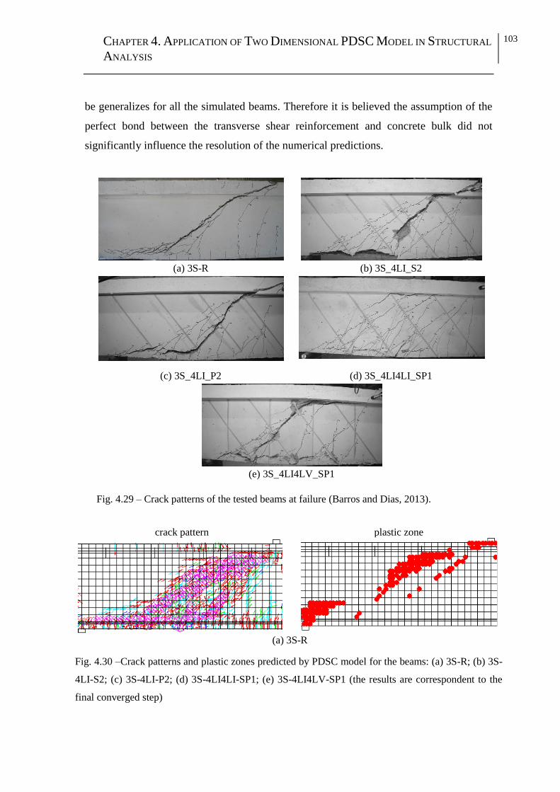
CHAPTER 4. APPLICATION OF TWO DIMENSIONAL PDSC MODEL IN STRUCTURAL
ANALYSIS
103
be generalizes for all the simulated beams. Therefore it is believed the assumption of the
perfect bond between the transverse shear reinforcement and concrete bulk did not
significantly influence the resolution of the numerical predictions.
(a) 3S-R (b) 3S_4LI_S2
(c) 3S_4LI_P2 (d) 3S_4LI4LI_SP1
(e) 3S_4LI4LV_SP1
Fig. 4.29 – Crack patterns of the tested beams at failure (Barros and Dias, 2013).
crack pattern plastic zone
(a) 3S-R
Fig. 4.30 –Crack patterns and plastic zones predicted by PDSC model for the beams: (a) 3S-R; (b) 3S-
4LI-S2; (c) 3S-4LI-P2; (d) 3S-4LI4LI-SP1; (e) 3S-4LI4LV-SP1 (the results are correspondent to the
final converged step)

CHAPTER 4. APPLICATION OF TWO DIMENSIONAL PDSC MODEL IN STRUCTURAL
ANALYSIS
104
crack pattern plastic zone
(b) 3S-4LI-S2
(c) 3S-4LI-P2
(d) 3S-4LI4LI-SP1
(e) 3S-4LI4LV-SP1
Fig. 4.30 – (Continued)

CHAPTER 4. APPLICATION OF TWO DIMENSIONAL PDSC MODEL IN STRUCTURAL
ANALYSIS
105
(a)
(b)
(c)
(d)
Fig. 4.31 – Experimental and numerical presentations of load-strain diagram for the beam 3S-4LI-
S2: (a) monitored laminates; (b) NSM laminate A; (c) NSM laminate B; (d) monitored still
stirrup.
Monitored laminate(Laminate B)
Monitored laminate(Laminate A)
Laminate A
SG_L2
SG_L1
SG_L3
SG_L4
0.2 0.4 0.6 0.8 1 1.2 1.4 1.60
100
200
300
400
500
600
Exp. Num.
SG_L3
SG_L1
SG_L3
SG_L4
SG_L1
SG_L2
SG_L4
SG_L2
Forc
e(k
N)
Strain in laminate A (%)
SG_L2
SG_L4
SG_L1
SG_L3
Laminate B0.2 0.4 0.6 0.8 1
0
100
200
300
400
500
600
Exp. Num.
SG_L3
SG_L1
SG_L3
SG_L4
SG_L1
SG_L2
SG_L4
SG_L2
Forc
e(k
N)
Strain in laminate B (%)
0.2 0.4 0.6 0.80
100
200
300
400
500
600
SG_S1
Fo
rce
(kN
)
Strain in the steel stirrup (%)
Num.
SG_S1
Exp.

CHAPTER 4. APPLICATION OF TWO DIMENSIONAL PDSC MODEL IN STRUCTURAL
ANALYSIS
106
4.2.6 Effect of fiber dosage and prestress level on shear behavior of RC beams
The experimental program (Soltanzadeh et al., 2016b) is composed of seven real-scale I
cross section beams of 4000 mm total length, L, and 500 mm cross section height, h.
These beams are categorized in two groups with, respectively, three and four members.
The cross sectional dimensions and arrangement of the reinforcements of the beams in
both, the first and second group, is illustrated in Fig. 4.32. The members of both groups
shared the same configuration and geometry, but featured different level of prestress (in
the first group of beams with three members) and fiber volume fraction (in the second
group of beams with four members). Two different shear spans, of 1475 mm and 1650
mm, were also adopted, respectively, for the beams of first and second group, as shown in
Fig. 4.32.
(a)
(b)
(c)
Fig. 4.32 - Geometry, reinforcement and test setup of the beams of (a) group 1 (G1-F1.1-S0; G1-
F1.1-S23; G1-F1.1-S46), (b) group 2 except G2-F0-ST, (c) G2-F0-ST (dimensions in mm)
(Soltanzadeh et al., 2016b).

CHAPTER 4. APPLICATION OF TWO DIMENSIONAL PDSC MODEL IN STRUCTURAL
ANALYSIS
107
The influence of prestressing the steel longitudinal reinforcements on the shear behavior
of the beams was studied by testing the three beams of the first group, while the four
beams of second group were tested to investigate the effect of fiber dosage on improving
the shear resistance of the developed elements. The beams in both groups were
longitudinally reinforced with one steel strand (15.2 mm diameter with a nominal cross
section of 140 mm2) of seven wires (of 5 mm diameter each, 5 ), and 2 GFRP rebars of
12 mm diameter, 12 , with ribbed surface. For the GFRP rebars elasticity modulus of 56
GPa (GFRPE =56 GPa), and tensile strength of 1350 (
,GFRP uf =1350 MPa) was reported at
the experimental program (Soltanzadeh et al., 2016b).
In the beams of the first group the level of prestress, solely applied to the steel strand, was
the main variable investigated. These beams were developed without conventional steel
stirrups by using the concrete composition SCC-F1.1 that includes 90 kg/m3 steel fibers
(equal to 1.1% of the concrete volume). The beams of the second group were developed
with constant level of prestress and different dosage of steel fibers, namely: 0%, 1.1%
and 1.5% in volume (or respectively 0, 90, 120 kg/m3 steel fibers in weight). The
concretes with 0% and 1.5% steel fibers are designated as SCC-F0 and SCC-F1.5,
respectively. Both the steel and GFRP reinforcements of this group (group 2) of the
beams were prestressed, the steel strand at 56% of its tensile strength (974 MPa, since the
tensile strength of the strand is 1740 MPa), while the two GFRP bars were prestressed at
30% of its tensile strength (405 MPa, since ,GFRP uf =1350 MPa). These beams of the
second group were developed without conventional steel stirrups except the beam G2-F0-
ST. The beam G2-F0-ST was reinforced with steel stirrup of 6 mm diameter, 6 , with
spacing of 130 mm. The steel stirrups had the elastic modulus of 200 GPa and yield, and
ultimate tensile strength of respectively 556 MPa and 682 MPa. Table 4.16 presents the
relevant characteristics of the beams of the first and second groups.
Eight-noded serendipity plane stress finite elements with 33 Gauss–Legendre IP scheme
were used for modeling the beams of both groups 1 and 2. In Fig. 4.33 is represented, as
an example, the finite element mesh used for the simulation of the beam G1-F1.1-S0. The
longitudinal steel strand and GFRP bars were modeled using 2-noded cable elements (one
degree-of-freedom per each node) with two IPs. The compressive reinforcement and steel

CHAPTER 4. APPLICATION OF TWO DIMENSIONAL PDSC MODEL IN STRUCTURAL
ANALYSIS
108
stirrups installed in the beam G2-F0-ST are meshed using 2-noded embedded cables with
two IPs. Perfect bond was assumed between the reinforcement bars/strand and the
surrounding concrete. For modeling the behavior of the steel reinforcement, the stress-
strain relationship represented in Fig. 4.3 was adopted. The values of the parameters that
define the stress-strain law (Fig. 4.3) for the steel strand, stirrups, and compressive
reinforcement are included in Table 4.17. The behavior of GFRP bar was modeled using
a linear-elastic stress-strain relationship. The prestress load was simulated by means of
temperature variation applied to the cable elements modeling the GFRP bars and steel
strand. Table 4.18 includes the values of the temperature variation applied for each
simulated beam. The values of the parameters used to define the constitutive law for
concretes SCC-F0, SCC-F1.1 and SCC-F1.5 are indicated in Table 4.19.
Table-4.16 Details of the beams in first and second group.
Specimen ID Concrete
type
Prestress level
fV
(%)
Stirrup Steel strand
(% of syf ;
stress level in
MPa)
GFRP
(% of ,GFRP uf ; stress
level in MPa)
Gro
up 1
G1-F1.1-S0 SCC-F1.1 0; 0 0 1.1 NO
G1-F1.1-S23 SCC-F1.1 23; 400 0 1.1 NO
G1-F1.1-S46 SCC-F1.1 46; 800 0 1.1 NO
Gro
up 2
G2-F0 SCC-F0 56; 974 30; 405 0 NO
G2-F0-ST SCC-F0 56; 974 30; 405 0 YES
G2-F1.1 SCC-F1.1 56; 974 30; 405 1.1 NO
G2-F1.5 SCC-F1.5 56; 974 30; 405 1.5 NO
Fig. 4.33 - Finite element mesh, load and support conditions used for analysis of the beam G1-
F1.1-S0.
plane stress element with 8 nodesLC
2D-cable element
(GFRP bars)
P/2
2D-cable element
(steel strand)

CHAPTER 4. APPLICATION OF TWO DIMENSIONAL PDSC MODEL IN STRUCTURAL
ANALYSIS
109
Table-4.17 Values of the parameters of the steel constitutive model.
Diameter
(mm) sy
(%)
sy
(N/mm2)
sh
(%) sh
(N/mm2)
su
(%) su
(N/mm2)
Third branch
exponent a 15.2 0.87 1740 0.87 1740 20.0 1917 1 b 10 0.28 566 1 594 10.0 661 1
c 6 0.278 556 1 583 10.0 682 1
a steel strand;
b compressive reinforcement;
c stirrups.
Table-4.18 General information about the simulation of the prestress load by means of
temperature variation.
Specimen ID
a
,t S
(MPa)
b
,t GFRP
(MPa)
c
( / ( ))mm mm C
d
ST
( )C
e
GFRPT
( )C
G1-F1.1-S0 - - - - -
G1-F1.1-S23 400 - 1 10-5
-200 -
G1-F1.1-S46 800 - 1 10-5
-400 -
G2-F0 974 405 1 10-5
-487 -723
G2-F0-ST 974 405 1 10-5
-487 -723
G2-F1.1 974 405 1 10-5
-487 -723
G2-F1.5 974 405 1 10-5
-487 -723 a
,t s thermal stress applied to the steel strand; b
,GFRPt thermal stress applied to the GFRP
bars; c coefficient of thermal expansion;
d( C)O
ST temperature variation applied to the
steel strand; e
( C)O
GFRPT temperature variation applied to the GFRP bars.
Note: the thermal strain and corresponding stress for the steel strand are calculated from:
,t S ST ; , ,t S S t SE . For the GFRP bars the following equations are taken:
,GFRPt GFRPT ;
, ,GFRPt GFRP GFRP tE .
To simulate the shear crack initiation and the degradation of crack shear stress transfer,
the shear softening diagram represented in Fig. 3.2 is assumed, and the values of the
parameters to define this diagram for each concrete are included in Table 4.19. For the
concretes SCC-F1.1 and SCC-F1.5 the same crack shear strength was used (,
cr
t p =1.75
MPa), while for the concrete SCC-F0 the value 1.2 MPa was adopted for ,
cr
t p . The shear
fracture energy for the concrete without steel fiber (concrete SCC-F0) was adopted as
,f sG =0.08 N/mm. For the concretes including the steel fibers (concretes SCC-F1.1 and
SCC-F1.5) higher values of ,f sG are adopted, as indicated in Table 4.19, to simulate the
effect of fiber reinforcement in resisting the degradation of shear stress transfer between
the faces of the cracks during the cracking process.

CHAPTER 4. APPLICATION OF TWO DIMENSIONAL PDSC MODEL IN STRUCTURAL
ANALYSIS
110
Table 4.19 – Values of the parameters of the concrete constitutive model for concretes SCC-F0,
SCC-F1.1, and SCC-F1.5.
Property Value
Poisson’s ratio 0.2
Young’s modulus
for SCC-F0 E=32100 2
N mm ;
for SCC-F1.1 E =33230 2
N mm ;
for SCC-F1.5 E =30580 2
N mm
Parameters defining the plastic-damage part
of the model
for SCC-F0: cf =66.45 N/mm
2 ;
,f cG =25 N/mm ; 1c =0.0035;
0 =0.4;
for SCC-F1.1: cf =67.05 N/mm
2 ;
,f cG =55
N/mm ; 1c =0.004;
0 =0.4;
for SCC-F1.5: cf =60.03 N/mm
2 ;
,f cG =65 N/mm ; 1c =0.004;
0 =0.4
Quadrilinear tension softening diagram (Fig.
3.1b)
for SCC-F0: ctf 3.25 N/mm
2;
fG 0.08 N/mm; 1 0.007;
1 0.3;
2 0.1; 2 0.15;
3 0.15; 3 0.05;
for SCC-F1.1: ctf 3.25 N/mm
2;
fG 6.0 N/mm; 1 0.0005;
1 0.75;
2 0.0025; 2 1.0;
3 0.1; 3 0.6;
for SCC-F1.5: ctf 3.25 N/mm
2;
fG 7.5 N/mm; 1 0.0005;
1 0.75;
2 0.0025; 2 1.0;
3 0.1; 3 0.6
Parameter defining the mode I fracture energy
available to the new crack (Sena-Cruz, 2004) 2
Parameters defining the crack shear stress-
crack shear strain softening diagram (Fig. 3.2)
for SCC-F0: ,
cr
t p 1.2 N/mm2; 0.4;
,f sG =0.08 N/mm;
for SCC-F1.1: ,
cr
t p 1.75 N/mm2; 0.2;
,f sG =1.5 N/mm;
for SCC-F1.5: ,
cr
t p 1.75 N/mm2; 0.2;
,f sG =2.0 N/mm
Crack bandwidth Square root of the area of Gauss integration
point
Threshold angle (Sena-Cruz, 2004) 30 degree
Maximum number of cracks per integration
point (Sena-Cruz, 2004) 2
Fig. 4.34 and Fig. 4.35 compare the numerical and the experimental load vs. mid-span
deflection for the beams of first and second groups, respectively. Fig. 4.36 represents the
experimental crack pattern of all the beams in both groups at the failure stage.

CHAPTER 4. APPLICATION OF TWO DIMENSIONAL PDSC MODEL IN STRUCTURAL
ANALYSIS
111
(a) (b)
(c)
Fig. 4.34 - Experimental and numerical load vs. mid-span deflection of the beams of the first
group: (a) G1- F1.1-S0; (b) G1- F1.1-S23; (c) G1- F1.1-S46.
In Fig. 4.37 is represented, as an example, the numerical crack pattern for the simulation
of the beams G2-F1.5 at the end of the analysis (at the end of the last converged loading
step). The figures 4.34 to 4.37 show that the numerical model is able to capture with good
accuracy the deformational response of the beams and the experimentally observed
profile of the failure crack. For all the beams the numerical peak load, max
NumF , predicted
by the model are compared with the experimental ones, maxF , in Table 4.20. The
information provided in Table 4.20 shows that the peak loads of all beams are closely
simulated with the average error of 6.07%.
0 10 20 30 40 50 60 70 800
50
100
150
200
250
300
Numerical
Experimental
L
oad
- P
(k
N)
Deflection (mm)
G1-F1.1-S0
0 10 20 30 40 50 60 70 800
50
100
150
200
250
300
Experimental
Numerical
L
oad
-P
(k
N)
Deflection (mm)
G1-F1.1-S23
0 10 20 30 40 50 60 70 800
50
100
150
200
250
300
Numerical
Experimental
L
oad
- P
(k
N)
Deflection (mm)
G1-F1.1-S46

CHAPTER 4. APPLICATION OF TWO DIMENSIONAL PDSC MODEL IN STRUCTURAL
ANALYSIS
112
(a) (b)
(c) (d)
Fig. 4.35 - Experimental and numerical load vs. mid-span deflection of the beams of the second
group: (a) G2- F0; (b) G2- F0-ST; (c) G2- F1.1; (d) G2-F1.5.
G1-F1.1-S0 (Reference) G1-F1.1-S23
G1-F1.1-S46
G2-F0 (Reference) G2-F0-ST
G2-F1.1 G2-F1.5
Fig. 4.36 – Crack pattern at failure of the first and second group of beams
(Soltanzadeh et al., 2016b).
0 10 20 30 40 50 60 70 800
50
100
150
200
250
300
Numerical
Experimental
Lo
ad -
P (
kN
)
Deflection (mm)
G2-F0
0 10 20 30 40 50 60 70 800
50
100
150
200
250
300
Numerical
Experimental
Lo
ad -
P (
kN
)
Deflection (mm)
G2-F0-ST
0 10 20 30 40 50 60 70 800
50
100
150
200
250
300
Numerical
Experimental
Lo
ad -
P (
kN
)
Deflection (mm)
G2-F1.1
0 10 20 30 40 50 60 70 800
50
100
150
200
250
300
Numerical
Experimental
Lo
ad -
P (
kN
)
Deflection (mm)
G2-F1.5

CHAPTER 4. APPLICATION OF TWO DIMENSIONAL PDSC MODEL IN STRUCTURAL
ANALYSIS
113
Fig. 4.37 - Numerical crack pattern predicted by PDSC model for the beam G2- F1.5 (The results
correspond to the final converged step).
Fig. 4.38 compares the numerical and the experimental load vs. strain (STIRRUPP )
relationship, where strain was registered in the location where the strain gauges SG4 and
SG5 were installed in the stirrups of the beam G2-F0-ST (see Fig. 4.32). This figure
indicates the both stirrups are already yielded at the failure stage of the beam G2-F0-ST,
which was also observed in the experimental program.
(a) (b)
Fig. 4.38 - Experimental and numerical load vs. strain in steel stirrups of beam G2-F0-ST.
The predicted GFRPP relationships (load versus strain obtained in the IP closest to the
mid-span of the beam) for all the beams, except for the G1-F1.1-S46 beam (due to
malfunctioning of the corresponding strain gauge), are compared with those of
experiments in Fig. 4.39.
P/2
0 10000 200000
100
200
300
( )Yielding of steel stirrup
STIRRUP
Numerical
Experimental
( )
L
oad
- P
(k
N)
strain of steel stirup -
Strain gauge No. SG4
2780sy
0 100000
100
200
300
( )Yielding of steel stirrup
STIRRUP
Numerical
Experimental
( )
L
oad
- P
(k
N)
strain of steel stirrp -
Strain gauge No. SG5
2780sy

CHAPTER 4. APPLICATION OF TWO DIMENSIONAL PDSC MODEL IN STRUCTURAL
ANALYSIS
114
Fig. 4.38 and Fig. 4.39 show the numerical simulations, in general, predict with good
accuracy the strain measured in the stirrups and GFRP bars, which means the assumption
of perfect bond between the steel stirrups and GFRP bars and surrounding concrete
adopted in these simulations, is acceptable. It should be aware that strains recorded by
strain gauges are quite dependent on their distance to the cracks crossing the
reinforcements where they are installed.
Table 4.20 – Details of the experimental results and the numerical analysis.
Specimen ID maxF
(kN)
max
NumF
(kN)
max max max/NumF F F
(%)
G1-F1.1-S0 240.12 221.04 7.9
G1-F1.1-S23 244.80 249.08 1.74
G1-F1.1-S46 245.6 251.53 2.41
G2-F0 229.52 207.63 9.53
G2-F0-ST 277.98 263.88 5.0
G2-F1.1 263 296.91 12.89
G2-F1.5 293.75 302.78 3.07
Average 6.07
(a) (b) (c)
(d) (e) (f)
Fig. 4.39 - Experimental and numerical load vs. GFRP strain at mid-span of the beams.
0 3000 6000 90000
50
100
150
200
250
300
GFRP
Numerical
Experimental
( )
L
oad
- P
(k
N)
GFRP strain at mid-span -
G1-F1.1-S0
0 3000 6000 90000
50
100
150
200
250
300
GFRP
Numerical
Experimental
( )
L
oad
- P
(k
N)
GFRP strain at mid-span -
G1-F1.1-S23
0 10000 200000
50
100
150
200
250
300
( )7230
GFRP
Numerical
Experimental
( )
L
oad
- P
(k
N)
GFRP strain at mid-span -
G2-F0
0 10000 200000
50
100
150
200
250
300
( )7230
GFRP
Numerical
Experimental
( )
L
oad
- P
(k
N)
GFRP strain at mid-span -
G2-F0-ST
0 10000 200000
50
100
150
200
250
300
( )7230
GFRP
Numerical
Experimental
( )
L
oad
- P
(k
N)
GFRP strain at mid-span -
G2-F1.1
0 10000 200000
50
100
150
200
250
300
( )7230
GFRP
Numerical
Experimental
( )
L
oad
- P
(k
N)
GFRP strain at mid-span -
G2-F1.5

CHAPTER 4. APPLICATION OF TWO DIMENSIONAL PDSC MODEL IN STRUCTURAL
ANALYSIS
115
The numerical relationships of the load vs. strain of steel strand at the beam’s mid-span (
STRANDP ) for all the developed beams are represented in Fig. 4.40 (the strain is
obtained at the IP closest to the mid-span of the beam). Fig. 4.40 shows that the steel
strand is not yielded in the control beam of the group 1 (the beam G1-F1.1-S0), while in
the beams G1-F1.1-S23 and G1-F1.1-S46 (the beams in group 1 and with prestress
applied to the steel strand) the steel strand has yielded at the loads about 230 kN.
(a) (b)
(c) (d)
(e) (f)
Fig. 4.40 - Numerical load vs. strain of strand in mid-span of the beams relationships.
0 6000 12000 180000
100
200
300
( )Yielding of steel strand
STRAND
Numerical
( )
L
oad
- P
(k
N)
strain of steel strand at mid-span -
G1-F1.1-S0
8700sy
0 6000 12000 180000
100
200
300 Deflection
( )
( )2000
Yielding of steel strand
STRAND
Numerical
( )
L
oad
- P
(k
N)
strain of steel strand at mid-span -
G1-F1.1-S23
8700sy
38mm
0 6000 12000 180000
100
200
300
( )
( )
4000
Yielding of steel strand
STRAND
Numerical
( )
L
oad
- P
(k
N)
strain of steel strand at mid-span -
G1-F1.1-S46
8700sy
Deflection 20.9mm
0 6000 12000 180000
100
200
300
( )
( )
4870
Yielding of steel strand
STRAND
Numerical
( )
L
oad
- P
(k
N)
strain of steel strand at mid-span -
G2-F0
8700sy
23.1mmDeflection
0 6000 12000 180000
100
200
300
( )
( )
4870
Yielding of steel strand
STRAND
Numerical
( )
L
oad
- P
(k
N)
strain of steel strand at mid-span -
G2-F0-ST
8700sy
16.9mmDeflection
0 6000 12000 180000
100
200
300
( )
( )
4870
Yielding of steel strand
STRAND
Numerical
( )
L
oad
- P
(k
N)
strain of steel strand at mid-span -
G2-F1.1
8700sy
Deflection 15.2mm

CHAPTER 4. APPLICATION OF TWO DIMENSIONAL PDSC MODEL IN STRUCTURAL
ANALYSIS
116
(g)
Fig. 4.40 – (Continued)
For the beams G2-F0 and G2-F0-ST, which are in the second group and made by
concrete SCC-F0, the steel strands has yielded at the load of about 200 kN. The predicted
strain in the strand at failure stage of the beam G2-F0-ST is about 77% higher than that of
the G2-F0, which is mainly due to the larger ultimate deflection of the beam G2-F0-ST.
For the beams in the second group and made by SFRSCC (the beams G2-F1.1 and G2-
F1.5), the yield initiation of steel strands has occurred at the load of about 240 kN. This
load is higher than those predicted for the beams made by concrete SCC-F0 (the beams
G2-F0 and G2-F0-ST), since the steel fibers bridging the flexural cracks crossing the steel
strand have contributed to decrease the average strain installed in the strand
(Mazaheripour et al., 2016).
Taking into account that the steel strand of the G1-F1.1-S0 beam was the unique to have
not yielded, the remaining beams can be considered as having failed in flexural-shear,
since the formation of a critical shear crack in these beams has occurred after yield
initiation of the steel strand and was caused by the strain-hardening character of this type
of steel, and the linear behavior and relatively high ultimate tensile strain of GFRP bars.
4.3 CONCLUSIONS
The constitutive model developed in chapter 3, was integrated in plane stress element of
the FEMIX computer code, which is a general purpose finite element program. The
chapter 4 is mainly dedicated to explore the potentialities of the proposed constitutive
model for the analysis of concrete and RC structures. The model is employed to simulate
0 6000 12000 180000
100
200
300
( )
( )
4870
Yielding of steel strand
STRAND
Numerical
( )
L
oad
- P
(k
N)
strain of steel strand at mid-span -
G2-F1.5
8700sy
Deflection 15.6mm

CHAPTER 4. APPLICATION OF TWO DIMENSIONAL PDSC MODEL IN STRUCTURAL
ANALYSIS
117
experimental tests that are governed by nonlinear phenomenon due to simultaneous
occurrence of cracking and inelastic deformation in compression. The simulated
examples cover a wide range of geometry of specimens, concrete type, loading
configurations, and reinforcement conditions.
The numerical simulations have predicted with good accuracy the load carrying capacity
ductility, crack pattern, plastic (compressive) zone, and failure modes of all types of
structures analysed. The results of these analyses indicate the robustness and accuracy of
the proposed model for simulating concrete and RC structures subjected to multi-axial
loading configurations.

CHAPTER 4. APPLICATION OF TWO DIMENSIONAL PDSC MODEL IN STRUCTURAL
ANALYSIS
118

C H A P T E R 5
THREE DIMENSIONAL PDSC MODEL:
FORMULATION AND APPLICATION IN STRUCTURAL
ANALYSIS
5.1 INTRODUCTION
Three dimensional FEM analyses can be simplified into two dimensional ones when
geometry of the structure under analysis and the distribution of loads allow the structure
to be treated as bi-dimensional body. In this case the two dimensional analysis can be
used to save the computational cost with sufficient accuracy. However in some cases, due
to specific geometry of the structure or the distribution of the loads, the two-dimensional
analyses are incapable to predict with sufficient accuracy the behaviour of the structures
under analysis, therefore three dimensional approaches should be used instead
The present chapter proposes a new three dimensional (3D) constitutive model for cement
based materials, based in the generalization of the two dimensional (2D) plastic-damage
multidirectional fixed smeared crack model (represented in chapter 3), allowing the
possibility of simulating its failure in structures with arbitrary geometry and dimensions.
The proposed model simulates the crack opening and shear sliding according to an
already existing 3D multidirectional fixed smeared crack model (Ventura-Gouveia et al.,
2008; Ventura-Gouveia, 2011). The model simulates the nonlinear compressive

CHAPTER 5. THREE DIMENSIONAL PDSC MODEL: FORMULATION AND
APPLICATION IN STRUCTURAL ANALYSIS
120
behaviour of concrete between the cracks using a numerical strategy that combines the
elasto-plasticity (plasticity) and damage theories.
Later in this chapter the three dimensional PDSC model was included in the 3D solid
element of the FEMIX computer code (Sena-Cruz et al., 2007; Ventura-Gouveia et al.,
2008), and its performance validated by simulating examples at the material and
structural levels. The numerical tool is employed to simulate the experimental tests of RC
column subjected to different eccentric loadings, RC beams made by different concrete
strength classes, and RC walls subjected to pure torsion. The predicted load carrying
capacity, ductility, crack pattern, plastic (compressive) zone, and failure modes of all
types of analysed structures are discussed and compared with the experimental data.
Finally, a parametric study is executed for highlighting the sensitivity of the numerical
simulations to the values adopted for the model parameters.
5.2 MODEL DESCRIPTION
5.2.1 Part of the model corresponding to the cracking process
To derive the constitutive equation of the proposed model, the additive decomposition of
the incremental strain vector, , into an incremental crack strain vector, cr , and an
incremental elastic strain vector, e , and an incremental plastic strain vector, p
, is
adopted (i.e. cr e p ). The incremental elastic strain vector is related to
the incremental stress vector, , according to the following constitutive equation:
( )e p cr
D (5.1)
Being 1 2 3 23 31 12{ , , , , , } the incremental stress vector induced into
the material due to 1 2 3 23 31 12{ , , , , , } and considering the constitutive
matrix of the intact material, eD .
The cr is obtained from the incremental local crack strain vector, cr
according to
the Eq. (2.32).

CHAPTER 5. THREE DIMENSIONAL PDSC MODEL: FORMULATION AND
APPLICATION IN STRUCTURAL ANALYSIS
121
where:
1 2, ,
Tcr cr cr cr
n t t (5.2)
with the subscripts n , 1t , and
2t indicating the axes of the local coordinate system of the
crack (see Fig. 5.1). The component cr
n is the mode I incremental crack normal strain,
while 1
cr
t and 2
cr
t are the sliding mode incremental crack shear strains in the
directions 1t and
2t , respectively.
Fig. 5.1 – Crack stress components, displacements and local coordinate system of the crack
(Ventura-Gouveia et al., 2008; Ventura-Gouveia, 2011).
At the crack zone of an IP, the opening and sliding process is governed by the following
crack constitutive relationship according to Eq. (2.35), (i.e. cr cr crD ).
where cr is the vector of the incremental crack stress in the crack coordinate system
with the contribution of normal, cr
n , and tangential components, 1
cr
t , 2
cr
t :
1 2, ,
Tcr cr cr cr
n t t (5.3)
x3
x2
x1
crack plane
x3
x2
x1
n
t1
t2
crack plane
tcr
s2
n
cr
w
s1
2 tcr
1

CHAPTER 5. THREE DIMENSIONAL PDSC MODEL: FORMULATION AND
APPLICATION IN STRUCTURAL ANALYSIS
122
Fig. 5.1 represents the components of the crack stress vector (i.e. cr
n , 1
cr
t , 2
cr
t ) in the
local coordinate system of the crack, and the corresponding displacements (i.e. w , 1s ,
2s
), being w the opening displacement, 1s the sliding displacement in
1t direction, and 2s
sliding displacement in 2t direction.
At the IP the equilibrium condition is assured by imposing the Eq. (2.37), (i.e.
cr crT ).
The matrix crD that includes the constitutive law of the active cracks, i.e., the ones not
completely closed, is defined as:
1
2
0 0
0 0
0 0
cr
n
cr cr
t
cr
t
D
D D
D
(5.4)
where cr
nD , 1
cr
tD and 2
cr
tD represent, respectively, the modulus corresponding to fracture
mode I (normal), sliding modulus in the 1t direction, and sliding modulus in the
2t
direction.
The crack normal stress, cr
n , and the modulus cr
nD are obtained from a
trilinear/quadrilinear diagram i.e. cr cr
n n law, like the one represented in Fig. 3.1.
The sliding modulus 1
cr
tD and 2
cr
tD can be simulated as:
1 2 1
cr cr
t t cD D G
(5.5)
where cG is the concrete elastic shear modulus, while the shear retention factor, , can
be a constant value or, alternatively, obtained by Eq. (3.6).
The cr cr
t t softening law (represented in Fig. 3.2) adopted to simulate more correctly
the shear stress transfer during the crack opening process (Ventura-Gouveia, 2011; Baghi

CHAPTER 5. THREE DIMENSIONAL PDSC MODEL: FORMULATION AND
APPLICATION IN STRUCTURAL ANALYSIS
123
and Barros, 2016; Soltanzadeh et al., 2016b). In this approach the crack shear stress (
1
cr
t or 2
cr
t ), and the modulus cr
tD are obtained from the cr cr
t t softening law. The
modulus of the first branch, ,1
cr
tD (see Fig. 3.2), is obtained according to Eq. (5.5) and
using a constant value in the range 0,1 for . For each crack shear component, the
crack shear strain at peak (1 ,
cr
t p or 2 ,
cr
t p ) is obtained using the crack shear strength ,
cr
t p and
the crack shear modulus ,1
cr
tD from the following equation (Ventura-Gouveia, 2011):
1 2
,
, ,
,1
cr
t pcr cr
t p t p cr
tD
(5.6)
The ultimate crack shear strain in each sliding directions (1 ,
cr
t u or 2 ,
cr
t u ) depends on the
shear fracture energy, ,f sG , crack shear strength,
,
cr
t p , and the crack bandwidth, bl , as
follows (Ventura-Gouveia, 2011):
1 2
,
, ,
,
2 f scr cr
t u t u cr
t p b
G
l
(5.7)
As demonstrated in the previous 2D version of the PDSC model (represented in chapter
3), for accurate predictions of the behavior of RC elements failing in shear, is
fundamental the adoption of a crack shear softening approach.
It should be noted the above-described equations are represented for the particular case of
only one crack per IP, however, the model is able to consider forming several cracks in
the same IP. The details corresponding to this development can be found elsewhere
(Ventura-Gouveia et al., 2008; Ventura-Gouveia, 2011).
5.2.2 Part of the model corresponding to the elasto-plasticity
The plastic strain vector, p , which appears in Eq. (5.1), is evaluated by a time-
independent plasticity model that is defined by four entities: yield function (yield

CHAPTER 5. THREE DIMENSIONAL PDSC MODEL: FORMULATION AND
APPLICATION IN STRUCTURAL ANALYSIS
124
surface); flow rule; evolution law for the hardening parameter; and conditions for
defining loading-unloading process. The plasticity part of the model is formulated in the
effective stress space, and accounts for the development of irreversible strains and
inelastic volumetric expansion of material under compression. To define the effective
stress space a distinction is made between the stress acting on damaged and undamaged
configurations of the material when subjected to a compression stress field. Effective
stress means the stress acting in the undamaged configuration of the material, defined as
the force divided by the undamaged area. Force divided by the total area (damaged plus
undamaged area) is called nominal stress (Edalat-Behbahani et al., 2015; Edalat-
Behbahani et al., 2016). Formulation of the plastic response in the effective stress space
implies the plasticity model do not account for the damage formed when the material is
loaded in compression. In this model, the state of damage in material under compression
is simulated in the framework of CDM as will be discussed in section 5.2.3.
For the three dimensional model, the equations describing yield function (Eq. (3.15)),
flow rule (Eq. (3.16)), evolution law for the hardening parameter (Eq. (3.17)), and
onditions for defining loading-unloading process (Eq. (3.18)) still hold in the form
deduced in section 3.3.3.
5.2.3 Part of the model corresponding to the damage process
In this model, the stiffness degradation and softening behaviour of concrete under
compression are simulated in the framework of CDM, in which the damage is considered
as an isotropic process. In this approach the state of damage in concrete under
compression is equally distributed in all directions, and can be represented by a scalar
measure, represented by cd . The scalar damage parameter
cd calculated according to Eq.
(3.54). The scalar damage parameter cd is used to map the effective stress vector ( )
into the nominal stress vector ( ) according to Eq. (3.14).
The coupling between the presented parts of the model and the corresponding obtained
system of nonlinear equations, that should be solved to update the local variables of the
3D PDSC model at a generic load increment of the incremental/iterative Newton–
Raphson algorithm generally adopted in FEM-based material nonlinear analysis, are

CHAPTER 5. THREE DIMENSIONAL PDSC MODEL: FORMULATION AND
APPLICATION IN STRUCTURAL ANALYSIS
125
similar to the described in the section 3.3.3.2 and 3.3.4 of the chapter 3 for the 2D PDSC
model.
5.3 SIMULATIONS AT THE MATERIAL LEVEL
The proposed model is initially validated by executing numerical tests at the material
level (single cube-shaped 8-noded solid element with one IP), which are intended as an
elementary verification of the basic capabilities of the model. The loading procedure of
the tests consists of imposing prescribed displacement increments and assuming the crack
bandwidth (bl ) equal to 100 mm. Since the concrete properties in each test were different,
the corresponding values are indicated in the caption of the figures.
- Simulation of cyclic compression-tension loading sequence (Fig. 5.2): The element is
initially loaded in compression, along the direction X2, up to a stage where the
concrete enters in the softening phase (1c c ). Due to compressive loading beyond
the uniaxial compressive strength of the concrete ( 30cf MPa), damage due to
inelastic compressive deformation is developed ( 0cd ). Then the element is unloaded
to tension and the unloading occurs with the damaged stiffness (1 )cd E , being E the
undamaged stiffness at the plasticity model. By increasing the tensile loading, a crack
(with the crack plane orthogonal to the loading direction X2) initiates and further
propagates. The element is then reloaded to compression, which causes the crack to be
gradually closed with a secant unloading branch. By increasing compressive loading
the crack is completely closed and later the response returns back to the softening
stage in compression. The loading procedure is continued for one more cycle of
compression-tension-compression, and the similar material response as that of the first
cycle was simulated. The response of the proposed model (in nominal stress space) is
compared in Fig. 5.2a with the solution reported at the work of Gernay et al. (2013).

CHAPTER 5. THREE DIMENSIONAL PDSC MODEL: FORMULATION AND
APPLICATION IN STRUCTURAL ANALYSIS
126
(a)
(b)
Fig. 5.2 – Simulation of cyclic compression-tension load sequence at the
material level (values for the parameters of the constitutive model: =0.2;
E =22 GPa; cf =30 MPa; ,f cG =7 N/mm; ctf =3 MPa; 1c =0.0025; 0 =0.3;
fG
=0.04 N/mm; 1 =0.2; 1 =0.7; 2 =0.75; 2 =0.2).
For comparison, Fig. 5.2b represents the response of the proposed model in nominal
stress space (represented at Fig. 5.2a) and the one in effective stress space. In
compression zone (2 0 ), the stress-strain responses in both effective and nominal
stress spaces are identical for the domain before attaining the peak (1c c ), whereas
for higher deformations (1c c ) the two responses starts diverging because of the
damage evolution process ( 0cd ). In tension zone, the simulated responses in both
effective and nominal stress spaces are also identical, since the compressive damage
-0.004 -0.003 -0.002 -0.001 0
-35
-30
-25
-20
-15
-10
-5
0
(-)
PDSC model (Nominal stress space)
Garney et al. (2013)
(MP
a)
2
2
2
22
2
2
2
2 2
X1
X3
X2
-0.004 -0.003 -0.002 -0.001 0
-40
-35
-30
-25
-20
-15
-10
-5
0
(MP
a)
PDSC model (Nominal stress space)
PDSC model (Effective stress space)
E
(1-dc)E
(-)

CHAPTER 5. THREE DIMENSIONAL PDSC MODEL: FORMULATION AND
APPLICATION IN STRUCTURAL ANALYSIS
127
scalar (cd ) only affects the negative (compressive) part of effective stress vector (
), (see Eq. (5.14)).
- Simulation of closing a crack developed in one direction, by imposing compressive
load in the orthogonal direction (Fig. 5.3): The element is initially subjected to the
uniaxial tension in the direction of X2 (Step 1).
Fig. 5.3 – Prediction of the PDSC model for closing a crack developed in one direction, by
imposing compressive load in the orthogonal direction (values for the parameters of the
constitutive model: =0.2; E =36 GPa; cf =30 MPa; ,f cG =30 N/mm; ctf =2.45 MPa; 1c
=0.0025; 0 =0.3; fG =0.05 N/mm; 1 =0.2; 1 =0.7; 2 =0.75; 2 =0.2).
Then a crack is formed with the orientation of 0º , and further propagated up to a
stage that the crack does not be able to transfer more tensile stresses (fully opened
crack status). At this stage the displacement in the direction of X2 is fixed (Step 2), and
the element is loaded by compressive displacements in the X3 direction up to end of
the analysis (Step 3).
-0.01-0.008-0.006-0.004-0.00200.002
-35
-30
-25
-20
-15
-10
-5
0
5
Cervenka & Papanikolaou (2008)
PDSC model
Str
ess
(MP
a)
Strain (-)
Crack is closed
Compressive strength fc
4
2
23
5
3
Second hardening-softening branches
)(
Biaxial compressive strength
5
4
1
1 First hardening-softening branches
Step3
Step2
Step1
3
3
2
X1
X3
X2
2

CHAPTER 5. THREE DIMENSIONAL PDSC MODEL: FORMULATION AND
APPLICATION IN STRUCTURAL ANALYSIS
128
Due to applied compressive displacements, uniaxial compressive stresses are induced
in the material in the X3 direction. Consequently, expansion of the material in the X2
direction imposes the crack be gradually closing. When the material is in the
compression softening phase, in X3 direction, the crack will be completely closed.
When the crack closes, the state of stress is changed to biaxial compression, and a
second hardening-softening response is reproduced corresponding to the appropriate
biaxial state of stress. The above-described loading path was successfully simulated by
the proposed model (see Fig. 5.3), and the prediction agrees well with the solution of
Cervenka and Papanikolaou (2008).
- Simulation of closing two cracks developed along two orthogonal directions, by
imposing compressive load in the third orthogonal direction (Fig. 5.4): The element is
initially subjected to equal tensile displacements along orthogonal directions X1 and
X2, therefore, two orthogonal cracks are developed (Step 1 in Fig. 5.4). The tensile
displacements are increased up to the stage that the two orthogonal cracks attain the
fully opened crack status.
At this stage the displacements of the elements in directions X1 and X2 are fixed (Step
2 in Fig. 5.4) and, simultaneously, compressive displacements are imposed in direction
X3 up to end of the analysis (Step 3 in Fig. 5.4). Due to compressive contraction in
direction X3, the material expands along X1 and X2 directions, consequently the both
existing cracks are gradually closing. When the material is in compressive softening
stage (in direction X3), both cracks become completely closed, and the state of stress in
direction X3 changes from uniaxial compression to triaxial compressive state. Fig. 5.4
presents the simulated loading path, and its comparison to the solution reported by
Cervenka and Papanikolaou (2008). A good agreement can be observed.

CHAPTER 5. THREE DIMENSIONAL PDSC MODEL: FORMULATION AND
APPLICATION IN STRUCTURAL ANALYSIS
129
Fig. 5.4 – Prediction of the PDSC model for closing two cracks developed along two
orthogonal directions, by imposing compressive load in the third orthogonal direction
(values for the parameters of the constitutive model adopted the same as those mentioned
in Fig. 5.3).
5.4 SIMULATIONS AT THE STRUCTURAL LEVEL
5.4.1 RC columns subjected to different eccentric loadings
To highlight the efficiency of the proposed model, three RC columns, here designated as
C-e0.3, C-e0.57, and C-e0.86 tested by El-Maaddawy (2009), were simulated. All the
specimens have the same geometry and reinforcement layout as represented in Fig. 5.5.
The test setup used for the execution of these tests is represented in Fig. 5.6. The test
specimen includes two end corbels, with the cross sections of 250250 mm and length of
350 mm, to transfer the load to the central region of the specimen, designated by “test
region”, which has the cross section of 125125 mm and length of 500 mm. The flexural
and shear reinforcement adopted for the end corbels are designed to ensure the damage
only occurs in the “test region” (El-Maaddawy, 2009). The differences between the
specimens C-e0.3, C-e0.57, and C-e0.86 are restricted only to the length of the
-0.006-0.004-0.00200.002
-50
-45
-40
-35
-30
-25
-20
-15
-10
-5
0
5
10
Cervenka & Papanikolaou (2008)
PDSC model
Str
ess
(MP
a)
Strain (-)
=
=
Crack is closed
Compressive strength fc
1
2
Hardening branch correspondingto triaxial compressive stresses
)(
4
1
First hardening-softening branches
3
2
1
3
4
Step3
Step2
Step1
1
1
2
X1
X3
X2
2
3
3

CHAPTER 5. THREE DIMENSIONAL PDSC MODEL: FORMULATION AND
APPLICATION IN STRUCTURAL ANALYSIS
130
eccentricity (e) of the load applied to each specimen. The value of “e” for the C-e0.3, C-
e0.57, and C-e0.86 is, respectively, 37.5, 71, and 107.5 mm that correspond to an
eccentricity length over the section height (e/h) ratios of 0.3, 0.57, and 0.86 (h=125 mm).
The longitudinal steel reinforcement in the “test region” consists of 4 steel bars of 10 mm
diameter while 6 mm diameter hoops are applied as the shear reinforcement. More details
about the geometry, reinforcing system and support conditions are indicated in Fig. 5.5
and Fig. 5.6.
Fig. 5.5 – Details of the test specimen (El-Maaddawy, 2009) (dimensions in mm).
FEM modelling of the concrete, and the loading steel plates are performed using twenty-
noded solid elements with 222 Gauss–Legendre integration scheme. The loading steel
plates are modeled as a linear-elastic material with Poisson’s coefficient of 0.3 and
elasticity modulus of 200 GPa. Fig. 5.7 represents, as an example, the finite element mesh
used for the simulation of the column C-e0.86 (the differences between each column test
are limited to the length of eccentricity for the load application). The longitudinal steel
bars and steel hoops are modeled with 3D embedded cables of 2 nodes (one degree-of-
5 No. 10T
est
reg
ion
2 No. 10
h = 125
No. 10 @ 70
No. 6
eP
35
0 5 No. 10
section B-B
2 No. 14
2 No. 14 25
0
250
B B
No. 6
250
section A-A
clear cover 15 mm
12
5A A
2 No. 10
12
51
25
50
03
50
12
51
25
4 No. 10
25
0
No. 10 @ 70
2 No. 14

CHAPTER 5. THREE DIMENSIONAL PDSC MODEL: FORMULATION AND
APPLICATION IN STRUCTURAL ANALYSIS
131
freedom per node), by using a 2 Gauss-Legendre integration scheme, and assuming
perfect bond to the surrounding medium.
Fig. 5.6 – Test set up (El-Maaddawy, 2009).
For modelling the behaviour of the steel bar elements, the stress-strain relationship
represented in Fig. 4.3 was adopted, and the values of parameters used to define this
diagram are included in Table 5.1. Properties of concrete are taken from (El-Maaddawy,
2009), and the values of the parameters to define the PDSC model are, accordingly,
included in Table 5.2. Elements of the top and bottom corbels are assumed exhibiting
linear elastic behaviour during the analysis, since no damage is reported for these
elements in the original papers. The applied load is uniformly distributed over the
appropriate edges of those elements of the top steel plate (see Detail A of Fig. 5.6), and
the simulation is performed under the displacement control by the arc-length method
considering the horizontal X2 translational degree of freedom of a point located at the
mid-height of tensile zone of the column.
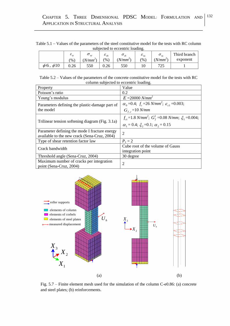
CHAPTER 5. THREE DIMENSIONAL PDSC MODEL: FORMULATION AND
APPLICATION IN STRUCTURAL ANALYSIS
132
Table 5.1 – Values of the parameters of the steel constitutive model for the tests with RC column
subjected to eccentric loading.
sy
(%)
sy
(N/mm2)
sh
(%) sh
(N/mm2)
su
(%) su
(N/mm2)
Third branch
exponent
6 , 10 0.26 550 0.26 550 10 725 1
Table 5.2 – Values of the parameters of the concrete constitutive model for the tests with RC
column subjected to eccentric loading.
Property Value
Poisson’s ratio 0.2
Young’s modulus E =20000 N/mm2
Parameters defining the plastic-damage part of
the model
0 =0.4; cf =26 N/mm
2;
1c =0.003;
,f cG =10 N/mm
Trilinear tension softening diagram (Fig. 3.1a) ctf =1.8 N/mm
2;
fG =0.08 N/mm; 1 =0.004;
1 = 0.4; 2 =0.1;
2 = 0.15
Parameter defining the mode I fracture energy
available to the new crack (Sena-Cruz, 2004) 2
Type of shear retention factor law P1 = 2
Crack bandwidth Cube root of the volume of Gauss
integration point
Threshold angle (Sena-Cruz, 2004) 30 degree
Maximum number of cracks per integration
point (Sena-Cruz, 2004) 2
(a) (b)
Fig. 5.7 – Finite element mesh used for the simulation of the column C-e0.86: (a) concrete
and steel plates; (b) reinforcements.
1X
3X
elements of column
elements of corbels
elements of steel plates
roller supports
2X
measured displacement
hU
hU
2X
3X

CHAPTER 5. THREE DIMENSIONAL PDSC MODEL: FORMULATION AND
APPLICATION IN STRUCTURAL ANALYSIS
133
The experimental relationship between the applied load versus the lateral mid-height
displacement (hP U ) of the column C-e0.3 is represented in Fig. 5.8a. This figure
includes the predicted hP U responses obtained by PDSC model and the SC model. The
SC model includes the same 3D multidirectional fixed smeared crack approach (Ventura-
Gouveia et al., 2008; Ventura-Gouveia, 2011) to account for cracking, but considers the
linear elastic behaviour for the material under compressive deformations.
(a)
(b) (c)
Fig. 5.8 – Experimental vs. numerical P-Uh responses (El-Maaddawy, 2009) for the specimen:
(a) C-e0.3; (b) C-e0.57; (c) C-e0.86.
According to the experimental observations, the column C-e0.3 exhibits a ductile hP U
response, and its failure was governed mainly by crushing of concrete at the compression
0 2 4 6 8 100
150
300
450
Load
-P
(kN
)
Lateral mid-height displacement - (mm)
Experimental
PDSC model
SC model
Linear analysis
Uh
0 2 4 6 8 10 120
50
100
150
Lo
ad-
P(k
N)
Lateral mid-height displacement - (mm)
Experimental
PDSC model
Uh
0 2 4 6 8 100
30
60
90
Lo
ad-
P(k
N)
Lateral mid-height displacement - (mm)
Experimental
PDSC model
Uh

CHAPTER 5. THREE DIMENSIONAL PDSC MODEL: FORMULATION AND
APPLICATION IN STRUCTURAL ANALYSIS
134
side of the column, without yielding of the longitudinal steel in the tensile side of the
specimen.
The experimental load vs. strain (,r tP ) relationships, where strain was recorded in
mid-height of the longitudinal steel reinforcement located at tensile zone, corresponding
to the column C-e0.3 is provided at Fig. 5.9a. This figure, Fig. 5.9a, indicates that the
strain in the reinforcement at failure stage is about ,tr 0.0008, which is less than the
strain corresponding to the yield initiation of steel bar (,t 0.0026r ).
(a) (b) (c)
Fig. 5.9 – Experimental vs. numerical ,r tP responses (El-Maaddawy, 2009) for the specimen:
(a) C-e0.3; (b) C-e0.57; (c) C-e0.86.
The numerical analysis using the SC model reveals that at the load corresponding to 40
kN the cracks in the tension-side of the column C-e0.3 are initiated (see Fig. 5.8a). Once
these cracks start to propagate, the stiffness of hP U response slightly decreases, but the
predicted load carrying capacity continuously increases without the occurrence of a
failure load, since the SC model assumes an elastic behaviour for the concrete in
compression. However, according to the PDSC response, after the initiation of the cracks
in the tension-side of the column, the hP U response is mainly governed by the
nonlinear compressive behaviour of concrete at compression side of the column.
Fig. 5.10b and 5.10c present, respectively, the numerical crack pattern and the plastic
zone, at the deformation corresponding to 9.2hU mm (last converged step). As can be
0 0.0005 0.001
08
01
60
24
0
Load
-P
(kN
)
Strain in tensile long. steel- (-)
PDSC model
sy = 0.0026
Yield initiation of steel
Experimental
r,t
at
0 0.001 0.002 0.003
05
01
00
15
0L
oad
-P(k
N)
Strain in tensile long. steel- (-)
PDSC model
sy = 0.0026
Yie
ldin
itia
tion
of
stee
l
Experimental
r,t
0 0.001 0.002 0.003
03
06
09
0L
oad
-P(k
N)
Strain in tensile long. steel- (-)
PDSC model
sy= 0.0026
Yie
ldin
itia
tio
no
fst
eel
Experimental
r,t

CHAPTER 5. THREE DIMENSIONAL PDSC MODEL: FORMULATION AND
APPLICATION IN STRUCTURAL ANALYSIS
135
seen in Fig. 5.10b, the cracks with large opening status are spread at the tension-side of
the column, while Fig. 5.10c shows the plastic zone is concentrated at the compression
side of the column. This numerical prediction correlates well with the experimental
observations (see Fig. 5.10a). The ,r tP response predicted by PDSC model, also,
confirms the longitudinal steel bars located in the tensile side of the column have not
yielded at the failure stage (see Fig. 5.9a).
(a) (b) (c)
Fig. 5.10 – Results of the specimen C-e0.3: (a) experimentally observed damage (El-Maaddawy,
2009); (b) numerical crack pattern and (c) plastic zone (results of (b) and (c) correspond to the
last converged step ( 9.2hU mm ).
According to the experimental program, the columns C-e0.57 and C-e0.86 have failed by
yielding of longitudinal tension steel and crushing of concrete at compression side of the
specimen (El-Maaddawy, 2009). Predictions of PDSC model for the columns C-e0.57
and C-e0.86 are represented in Fig. 5.8 and Fig. 5.9 in terms of hP U and
,r tP
relationships, respectively. As can be in seen in these two figures the PDSC model was
able to predict with good accuracy the overall experimental hP U and
,r tP

CHAPTER 5. THREE DIMENSIONAL PDSC MODEL: FORMULATION AND
APPLICATION IN STRUCTURAL ANALYSIS
136
responses of the columns C-e0.57 and C-e0.86. The predicted ,r tP relationships for
both columns confirm the tensile longitudinal steel bars are already yielded at their failure
stages. By comparing the experimental hP U and
,r tP responses of the three
columns, it can be concluded that by increasing the e/h ratio the failure load decreases
whereas the strains in tensile longitudinal reinforcement bars increase. This experimental
observation was successfully simulated by the PDSC model as revealed in Fig. 5.8 and
Fig. 5.9.
5.4.2 RC beams made by different concrete strength classes
The proposed model is applied in this section on the simulation of RC beams made by
different concrete strength classes, tested by Yang et al. (2003). The six beams analysed:
L-60, L-75, L-100, H-60, H-75, H-100, have the same shear span over cross-section depth
ratio (a/h) and thickness (b). Fig. 5.11 and Table 5.3 provide the relevant information
about these beams. The tensile longitudinal reinforcement ratio for all the beams is about
1.0%, applied in one or two layers, while no shear reinforcement at the shear spans is
adopted for these beams. The tensile reinforcement consists of steel bars of 19 mm
diameter and 22 mm diameter, with a total cross sectional area represented by Ast in Table
5.3.
Fig. 5.11 – Geometry and reinforcement layout for the beams tested by Yang et al.
(2003) (dimensions in mm).
( 100 10)b
steel plate
steel plate
L
d
stA
15
25
100100
2 No. 10
b
2l aaa
150150l
h
total area of
( 100 10)b

CHAPTER 5. THREE DIMENSIONAL PDSC MODEL: FORMULATION AND
APPLICATION IN STRUCTURAL ANALYSIS
137
Table 5.3 – Details of the beams tested by Yang et al. (2003).
ID group cf
(MPa)
h
(mm)
a
(mm)
d
(mm) L
(mm)
l
(mm) stA (a)
(mm2)
Web
Reinf.
a/h
(-)
b
(mm)
L-60 L 31.4 600 300 555 2400 2100 861
No 0.5
160
H-60 H 78.5 600 300 555 2400 2100 861 160
L-75 L 31.4 750 375 685 1650 1350 1148 160
H-75 H 78.5 750 375 685 1650 1350 1148 160
L-100 L 31.4 1000 500 935 1900 1600 1348 160
H-100 H 78.5 1000 500 935 1900 1600 1348 160
(a)stA : 861 (= 3 No. 19); 1148 (= 4 No. 19); 1348 (= 2 No. 19 + 2 No. 22)
In order to prevent flexural failure by the yielding of tension bars prior to shear failure,
some of the bars (namely those of 19 mm diameter) were of high tensile strength. Two
steel bars of 10 mm diameter were used as compressive reinforcements for all the beams.
The properties of the steel bars are indicated in Table 5.4. The beams can be assembled in
two groups according to the concrete strength level: L group that contains the beams of
concrete strength of 31.4 MPa (cf =31.4 MPa); and H group formed by the beams made
by high strength concrete (cf =78.5 MPa). Each group (L or H) contains three beams that
differ on the overall depth of the cross section (h=600, 750, or 1000 mm), while all the
beams have the same a/h ratio equal to 0.5.
Twenty-noded solid elements with 333 Gauss–Legendre integration scheme were used
for modelling the beams, supports and loading plates. Fig. 5.12 presents, as an example,
the finite element mesh used for the simulation of the beam L-75. The steel reinforcement
is modelled by 2-noded perfect bonded embedded cables with two IPs. For modelling the
behaviour of the steel bar elements, the stress-strain relationship represented in Fig. 4.3
was adopted, whose defining values are included in Table 5.4.
Support and loading plates are modeled as a linear-elastic material with Poisson’s
coefficient of 0.3 and elasticity modulus of 200 GPa. Properties of both regular and high
strength concrete (cf =31.4 MPa,
cf =78.5 MPa) are taken from Yang et al. (2003), and
the values of the parameters to define the PDSC model are, accordingly, included in
Table 5.5.

CHAPTER 5. THREE DIMENSIONAL PDSC MODEL: FORMULATION AND
APPLICATION IN STRUCTURAL ANALYSIS
138
Fig. 5.12 – Finite element mesh used for the simulation of the beam L-75
(due to symmetry conditions only half beam was modelled).
For the concrete with cf =31.4 MPa the value of ,f cG = 10 N/mm was considered, which is
the lower limit of the interval values proposed by Vonk (1992). For the high strength
concrete the average value of the interval proposed by Vonk (1992) was assumed (,f cG =
15 N/mm). To simulate the shear crack initiation and the degradation of crack shear stress
transfer, the shear softening diagram represented in Fig. 3.2 is assumed, and the values of
the parameters to define this diagram are included in Table 5.5. Due to lack of reliable
experimental evidences to characterise this diagram, the adopted values were estimated
taking into account the results obtained in previous simulations with RC beams failing in
shear, as well as the influence of the concrete strength class in the values of these
parameters (Barros et al., 2016; Baghi and Barros, 2016; Edalat-Behbahani et al., 2015).
Table 5.4 – Values of the parameters of the steel constitutive model for modelling the beams
tested by Yang et al. (2003).
Bar
diameter sy
(%)
sy
(N/mm2)
sh
(%)
sh
(N/mm2)
su
(%)
su
(N/mm2)
Third branch
exponent
22 0.21 407 2.5 420 10 553 1
19 0.413 804 1.3 808 10 890 1
10 0.209 408 1.42 412 4.4 549 1
3X
1X
2X
roller supports
elements of steel
plates
elements of concrete

CHAPTER 5. THREE DIMENSIONAL PDSC MODEL: FORMULATION AND
APPLICATION IN STRUCTURAL ANALYSIS
139
Table 5.5 – Values of the parameters of the concrete constitutive model for simulating the beams
tested by Yang et al. (2003).
Property Group Value
Poisson’s ratio L, H =0.15
Young’s modulus L E =27000 N/mm
2
H E =39000 N/mm2
Parameters defining the plastic-
damage part of the model
L 0 =0.4;
cf =31.4 N/mm2;
1c =0.0025;
,f cG =10 N/mm
H 0 =0.4;
cf =78.5 N/mm2;
1c =0.0035;
,f cG =15 N/mm
Trilinear tension softening
diagram (Fig. 3.1a)
L ctf =1.8 N/mm
2;
fG =0.07 N/mm; 1 =0.005;
1 =
0.3; 2 =0.1;
2 = 0.15
H ctf =2.0 N/mm
2;
fG =0.08 N/mm; 1 =0.005;
1 =
0.3; 2 =0.1;
2 = 0.15
Parameter defining the mode I
fracture energy available to the
new crack (Sena-Cruz, 2004)
L, H 2
Parameters defining the crack
shear stress-crack shear strain
softening diagram (Fig. 3.2)
L, H ,
cr
t p =1.2 N/mm2; =0.1 ;
,f sG =0.08 N/mm
Crack bandwidth L, H Cube root of the volume of Gauss integration point
Threshold angle (Sena-Cruz,
2004) L, H 30 degree
Maximum number of cracks
per integration point (Sena-
Cruz, 2004)
L, H 2
The relationships between the applied force and the mid-span displacement, F-U, for all
the beams, registered experimentally and obtained numerically with the PDSC model, are
represented in Fig. 5.13.
According to the experimental observations, all the beams exhibited large load carrying
capacity after the formation of the first diagonal crack, due to the resisting mechanism
ensured by the compressive strut connecting the loading points and the supports. The
experimental cracking patterns of all beams at the failure stage demonstrated the
formation of flexural cracks with very small crack width in middle of the beam, whereas
highly propagated diagonal cracks were observed along the line connecting the support
and loading plates. All beams failed by crushing of concrete compressive strut in brittle

CHAPTER 5. THREE DIMENSIONAL PDSC MODEL: FORMULATION AND
APPLICATION IN STRUCTURAL ANALYSIS
140
and sudden manner (Yang et al., 2003). In Fig. 5.14 is represented, as an example, the
experimental cracking patterns of the beams H-60 at its failure stage, while the same
pattern was observed for the other beams at the test (Yang et al., 2003).
(a) (b) (c)
(d) (e) (f)
Fig. 5.13 – Experimental (Yang et al., 2003) and numerical load vs. mid-span deflection
for the beams: (a) L-60; (b) L-75; (c) L-100; (d) H-60; (e) H-75; (f) H-100.
Table 5.6 gives the failure loads of the beams obtained in the experimental program ( expF
) and in the numerical simulations ( numF ), where it is verified that PDSC model was able
to simulate, with high accuracy, the experimental failure loads with an average error of
5.13% (see Table 5.6).
0 1 2 3 4 50
400
800
1200
PDSC model
Experimental
L-60
Tota
llo
ad-
F(k
N)
Mid-span deflection - (mm)U0 1 2 3
0
400
800
1200
PDSC model
Experimental
L-75
Tota
llo
ad-
F(k
N)
Mid-span deflection - (mm)U0 1 2 3
0
400
800
1200
PDSC model
Experimental
L-100
Tota
llo
ad-
F(k
N)
Mid-span deflection - (mm)U
0 1 2 3 4 5 60
400
800
1200
1600
2000
PDSC model
Experimental
H-60
Tota
llo
ad-
F(k
N)
Mid-span deflection - (mm)U
0 1 2 30
400
800
1200
1600
2000
PDSC model
Experimental
H-75
Tota
llo
ad-
F(k
N)
Mid-span deflection - (mm)U0 1 2 3
0
400
800
1200
1600
2000
PDSC model
Experimental
H-100T
ota
llo
ad-
F(k
N)
Mid-span deflection - (mm)U

CHAPTER 5. THREE DIMENSIONAL PDSC MODEL: FORMULATION AND
APPLICATION IN STRUCTURAL ANALYSIS
141
(a) (b)
(c)
Fig. 5.14 – Results of the beam H-60: (a) experimental crack patterns; (b) numerical
crack pattern; (c) plastic zone (for (b) and (c) the damage stages are obtained at the last
converged step).
By comparing expF of the beams with the same cross section depth but of different
concrete compressive strength, it can be concluded the increase of cf from 31.4 to 78.5
MPa resulted in an average increase of 66% in the failure loads. This experimental
observation was successfully captured by the PDSC model, as shown in Table 5.6 and
Fig. 5.13. This figure also shows that the PDSC model fit with high accuracy the
experimental F U curves at all stages of loading till failure. Fig. 5.14b shows that the
diagonal cracks at the last converged step of the analysis are in the full opening status
(cracks in pink colour), which means that the cracks are not capable of transferring any
type of stresses, while the simulated plastic zone for this beam (Fig. 5.14c) evidences the
formation of the compressive struts connecting the loading points and supports.

CHAPTER 5. THREE DIMENSIONAL PDSC MODEL: FORMULATION AND
APPLICATION IN STRUCTURAL ANALYSIS
142
Table 5.6 – Experimental and numerical failure loads of the beams.
ID group expF
(kN)
numF
(kN)
exp
exp
numF F
F
(%)
L-60 L 1070.2 1047.8 2.09
H-60 H 1646.4 1583.6 3.81
L-75 L 1193.6 1140.7 4.43
H-75 H 2020.8 1841.6 8.86
L-100 L 1164.2 1144.3 1.7
H-100 H 2058.0 1854.1 9.9
average 5.13
5.4.3 RC wall subjected to pure torsion
In this section the PDSC model is used for simulating reinforced concrete walls under
pure torsion loading configuration, tested by Peng and Wong (2011). The walls that were
designated by S8, S10 in the experimental program were selected for the numerical
simulations. The experimental loading procedure introduces the horizontal-pushing forces
F1 and F2 (the force F2 acts in the opposite direction of F1) to produce a torque on the
wall specimens. The magnitude of the forces F1 and F2 at the experimental program was
almost identical varying in the range of 1 kN (Peng and Wong 2011). The distance
between the two pushing forces was 500 mm. These walls had relatively thick slabs (with
the dimension of 1250 mm ×750 mm ×200 mm) at their bottom and top edges for fixing
the walls to the foundation, and for applying the forces (F1 and F2), respectively (see Fig.
5.15).
The walls are reinforced in both vertical and horizontal directions with the reinforcement
ratios designated as v and
h , respectively (see Table 5.7). Both walls have the same
thickness, tw, and height, hw, as indicated in Table 5.7, and are made of a concrete with a
compressive strength of 29.5 MPa. Details corresponding to the reinforcement applied in
horizontal and vertical directions are included in Table 5.7. The primary variable of these
two walls is the length of the wall (lw): the lw of S8 and S10 is, respectively, 800 mm and
1000 mm.

CHAPTER 5. THREE DIMENSIONAL PDSC MODEL: FORMULATION AND
APPLICATION IN STRUCTURAL ANALYSIS
143
Fig. 5.15 – General arrangement of the wall specimens tested by Peng and Wong (2011)
(dimensions in mm)..
Table 5.7 – Details of the RC walls submitted to torsion.
ID wt
(mm)
wh
(mm) wl
(mm)
(1)Vertical reinforcement
(5)Horizontal reinforcement
(2)N
(3)D
(mm)
(4)v
(%)
(6)D
(mm)
(7)Sh
(mm)
(8)h
(%)
S8 150 1500 800 9 10 1.18 8 125 0.57
S10 150 1500 1000 8 12 1.2 10 200 0.55
(1) vertical reinforcement is applied in two layers; (2) number of bars applied in each layer of
vertical reinforcement; (3) diameter of each bar in vertical reinforcement; (4) vertical
reinforcement ratio; (5) horizontal reinforcement was applied in the form of the rectangular
hoop; (6) diameter of one leg of each stirrup; (7) spacing of the stirrups; (8) horizontal
reinforcement ratio.
The test setup used for execution these tests is represented in Fig. 5.16a. Figs. 5.16b and
16c indicate the arrangement of linear variable displacement transducers (LVDTs) used to
measure the twist angle per unit length ( ) of these walls. As can be seen in these figures,
four LVDTs (designated by 3iL ,
3 jL , 2iL ,
2 jL ) are installed at two height levels (here is
called “level 2” and “level 3”) of each wall. The twist angle per unit length ( ) was
F2
F1
300
300
Steel transfer
plates
Face C
Face D
Face A
wt
wh
750
1250
200
wl

CHAPTER 5. THREE DIMENSIONAL PDSC MODEL: FORMULATION AND
APPLICATION IN STRUCTURAL ANALYSIS
144
calculated at the experimental program by using the measured data of these four LVDTs
according to the following equation:
3 3 2 2arctan( ) arctan( ) /
i j i j
h
l l
L L L Ld
d d
(6.1)
where the values of hd and
ld are defined in Fig. 5.16c.
(a) (b)
(c)
Fig. 5.16 – Setup for the test of shear walls subjected to torsion (Peng and
Wong, 2011).
Fo
r b
oth
wal
ls d
h=
75
0 m
mFace D
Level 3
represents LVDT
For the wall S10 dl=920 mm
For the wall S8 dl=720 mm
3 jL3iL
2 jL
Mea
surm
ent
len
gth
(d
h)
Face BFace A
2iL
Distance between
two LVDTs (dl)
For both walls dh=750 mm
Level 2

CHAPTER 5. THREE DIMENSIONAL PDSC MODEL: FORMULATION AND
APPLICATION IN STRUCTURAL ANALYSIS
145
FEM modelling of the walls, top slabs and steel plates were performed using twenty-
noded solid finite elements with 333 Gauss-Legendre IP scheme. Fig. 5.17 presents, as
an example, the finite element mesh used for analysis of the wall S10. Instead of
modelling the foundation, all the degrees-of-freedom of the bottom nodes of the walls are
considered fixed. The loads F1 and F2 are uniformly distributed over the appropriate
faces of the steel plate elements, as schematically represented in Fig. 5.17. The loading
steel plates are modeled as a linear-elastic material with Poisson’s coefficient of 0.3 and
elasticity modulus of 200 GPa. Elements of the top slab are assumed to exhibit linear
elastic behaviour during the analysis, since no damage is reported for this RC Slab in the
original paper. For modelling the behaviour of the steel bars, the stress-strain relationship
represented in Fig. 4.3 was adopted. The reinforcement is meshed using 2-noded perfect
bonded embedded cables with two IPs.
Fig. 5.17 – Finite element mesh used for the simulation of the wall S10.
The values of parameters used to define the constitutive models of steel and concrete are
included in Table 5.8 and Table 5.9, respectively. For modelling the shear stress transfer
1X
2X
elements of the steel
plates
elements of the RC wall
elements of the RC top
slab
roller supports
3X

CHAPTER 5. THREE DIMENSIONAL PDSC MODEL: FORMULATION AND
APPLICATION IN STRUCTURAL ANALYSIS
146
during the crack opening process, the crack shear softening law (Fig. 3.2) was adopted,
whose defining values are included in Table 5.9. Fig. 5.18 shows the experimental torque
vs. twist angle per length (T ) relationships for both walls and the respective
numerical predictions with the PDSC model. According to the experimental observations,
these walls exhibit ductile T responses after the crack initiation, and their failure
were governed by the formation of diagonal cracks inclined about 45° to the vertical axis.
Fig. 5.19 represents, as an example, the experimental crack pattern of the S8 wall at its
failure stage and the respective numerical prediction. For both walls the ductility and the
torque carrying capacity are predicted by the PDSC model with good accuracy, although
a slight higher torque was obtained numerically, mainly in the Wall S10. The numerical
crack pattern shows that the inclined cracks with highly propagated opening status are
spread over all faces of the wall which is in agreement with the experimental observation.
Table 5.8 – Values of the parameters of the steel constitutive model for the test of RC walls.
sy
(%)
sy
(N/mm2)
sh
(%)
sh
(N/mm2)
su
(%)
su
(N/mm2)
Third branch
exponent
8 0.228 422 0.2284 422 10 574 1
10 0.253 450 0.253 450 10 576 1
12 0.261 481 0.261 481 10 600 1
Table 5.9 – Values of the parameters of the concrete constitutive model for the test of RC walls.
Property Value
Poisson’s ratio 0.2
Young’s modulus E =26000 N/mm2
Parameters defining the plastic-damage part of
the model
0 =0.4; 1c =0.003;
,f cG =10 N/mm ;
cf =29.5 N/mm2
Trilinear tension softening diagram (Fig. 3.1a) ctf =2.0 N/mm
2;
fG =0.07 N/mm;
1 =0.006; 1 = 0.3;
2 =0.2; 2 = 0.1
Parameter defining the mode I fracture energy
available to the new crack (Sena-Cruz, 2004) 2
Parameters defining the crack shear stress-
crack shear strain softening diagram (Fig. 3.2) ,
cr
t p =1.2 N/mm2; =0.3 ;
,f sG =0.07 N/mm
Crack bandwidth Cube root of the volume of Gauss integration
point
Threshold angle (Sena-Cruz, 2004) 30 degree
Maximum number of cracks per integration
point (Sena-Cruz, 2004) 2
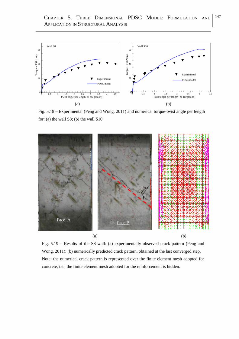
CHAPTER 5. THREE DIMENSIONAL PDSC MODEL: FORMULATION AND
APPLICATION IN STRUCTURAL ANALYSIS
147
(a) (b)
Fig. 5.18 – Experimental (Peng and Wong, 2011) and numerical torque-twist angle per length
for: (a) the wall S8; (b) the wall S10.
(a) (b)
Fig. 5.19 – Results of the S8 wall: (a) experimentally observed crack pattern (Peng and
Wong, 2011); (b) numerically predicted crack pattern, obtained at the last converged step.
Note: the numerical crack pattern is represented over the finite element mesh adopted for
concrete, i.e., the finite element mesh adopted for the reinforcement is hidden.
0 0.5 1 1.5 2 2.5 3 3.5 4 4.50
20
40
60
Twist angle per length - (degree/m)
Experimental
PDSC model
Wall S8
To
rque
-T
(kN
.m)
0 0.5 1 1.5 2 2.5 3 3.5
0
20
40
60
Twist angle per length - (degree/m)
Experimental
PDSC model
Wall S10
To
rque
-T
(kN
.m)
Face AFace B

CHAPTER 5. THREE DIMENSIONAL PDSC MODEL: FORMULATION AND
APPLICATION IN STRUCTURAL ANALYSIS
148
5.5 PARAMETRIC STUDY FOR THE MODEL PARAMETERS
A parametric study is performed to assess the influence of the values of the model
parameters on the simulated behaviour of the structures analyzed in the previous section
(section 5.4). The parameters under consideration are those simulating the nonlinear
behaviour of concrete under compression (cf ,
,f cG , 1c ), and those used to define the
crack shear softening diagram (,
cr
t p ,,f sG , ). To assess the influence of the parameters
cf
,,f cG and
1c the RC beam L-75 was chosen since its failure behavior is governed mainly
by crushing of the compressive strut. The RC wall S10 was selected to study the
influence of the parameters ,
cr
t p , ,f sG , , because the influence of the crack shear
softening diagram, which simulate the degradation of the shear stress transfer between the
faces of the crack, is significant to predict correctly the deformational and cracking
behaviour of this wall.
5.5.1 Influence of cf
Three different values for cf were adopted, 20, 31.4 and 40 N/mm
2 in the simulations of
the L-75 beam, the first one is lower than the value considered in the analysis of Section
5.4.2 (cf =31.4 N/mm
2), while the third is higher.
Fig. 5.20a indicates that the beam’s stiffness and the load carrying capacity increase with
cf . As expected, the SC model predicts a much higher ultimate load since the concrete in
compression is assumed having a linear behaviour.
The stages where the effect of inelastic compressive deformation becomes relevant on the
force-deflection responses of the beam in analysis are indicated in Fig. 5.20a using
markers. It is verified that these markers are localized in the force-deflection response of
this beam when predictions with the PDSC model start diverging from that of SC model.
The higher is the concrete compressive strength the larger is the load carrying capacity of
the beam corresponding to the marker, which is justified by the adoption of a constant
value for the 0 parameter, which defines the initiation of the inelastic deformation of
concrete in compression (0 0c cf f ). Since experimental research demonstrates (Hassan

CHAPTER 5. THREE DIMENSIONAL PDSC MODEL: FORMULATION AND
APPLICATION IN STRUCTURAL ANALYSIS
149
et al., 2012) the amplitude of the initial linear-elastic branch of the uniaxial compressive
behaviour increases with the concrete compressive strength (and consequently 0
increases with cf ), the initiation of the influence of the concrete inelastic compressive
deformation in the response of the beam will be postponed for larger deflection.
(a) (b) (c)
Fig. 5.20 – Sensitivity of the analysis of the beam L-75 with respect to the values
of the parameters: (a) cf ; (b)
1c ; (c) ,f cG .
5.5.2 Influence of 1c
To assess the influence of the parameter 1c on the response of the beam in analysis,
three values were considered, 0.0018, 0.0025 and 0.0035, the first one is lower than the
value considered in the analysis executed in Section 5.4.2 (1c =0.0025), while the third
value is higher. The parameter 1c influences both plasticity and damage parts of the
PDSC model. Within the plasticity part, the value of the hardening parameter at
compressive strength, 1c, is calculated according to Eq. (3.19) by attributing a certain
value to 1c . According to this equation
1c follows the tendency of
1c , therefore the
pre-peak branch (hardening phase) of the 1c c diagram is as stiffer as smaller is
1c ,
as shown in Fig. 3.6a. According to the PDSC model, the damage threshold is assumed to
be related to 1c: when
1c c , 0cd , while for 1c c the scalar damage parameter is
0 1 2 30
400
800
1200
1600
PDSC model with
L-75
Tota
llo
ad-
F(k
N)
Mid-span deflection - (mm)
PDSC model with
PDSC model with
fc
=40 MPa
Initiation of nonlinearcompressivedeformation
fc
=31.4 MPa
=20 MPa
fc
SC model
U
0 1 2 30
400
800
1200
PDSC model with
L-75
Tota
llo
ad-
F(k
N)
Mid-span deflection - (mm)
PDSC model with
PDSC model with c1
= 0.0035
c1
= 0.0025
c1
= 0.0018
U0 1 2 3
0
400
800
1200
PDSC model with
L-75
Tota
llo
ad-
F(k
N)
Mid-span deflection - (mm)
PDSC model with
PDSC model withGf,c=17 N/mm
=10 N/mm
=5 N/mm
Gf,c
Gf,c
U

CHAPTER 5. THREE DIMENSIONAL PDSC MODEL: FORMULATION AND
APPLICATION IN STRUCTURAL ANALYSIS
150
0cd . Since 1c increases with
1c , the occurrence of damage (i.e. 0cd , which
characterize the entrance of concrete in its compressive strain softening stage), initiates at
higher compressive deformation. These effects are reflected in the deformational
behaviour of the beam, since its stiffness in the initial force-deflection stage has
decreased with the increase of 1c (Fig. 5.20b). However, the entrance in the post-peak
concrete compressive softening stage is postponed with the increase of 1c , resulting a
increase of the beam’s ductility and load carrying capacity at the ultimate stage. This
means that by increasing 1c the stiffness of the load vs. deflection response decreases,
but the ultimate load, and its deflection increase, with benefits in terms of the ductility
response and load capacity of the beam.
5.5.3 Influence of ,f cG
The parameter of compressive fracture energy (,f cG ) controls the rate of strain softening
in compression, i.e. the level of stress decrease with the increase of compressive strain
(see Fig. 3.6c). As larger is ,f cG as smoother is this stress decay, which is a characteristic
of very ductile materials like fibre reinforced concrete (Barros and Sena-Cruz, 2001). Fig.
5.20c compares the force-deflection responses obtained for three different values of the
,f cG , 5, 10 and 17 N/mm, the first one is lower than the value considered in the analysis
of Section 5.4.2 (,f cG =10 N/mm), while the third is higher. Fig. 5.20c shows that the
parameter ,f cG influences the force-deflection response of the beam only after the
deflection of 1.7 mm, which corresponds to the deflection stage above that the effect of
strain softening behaviour of concrete under compression becomes relevant. By
increasing ,f cG the ultimate load capacity and deflection performance are increased.
5.5.4 Influence of ,
cr
t p
Fig. 5.21a represents the influence of the parameter ,
cr
t p on the torque vs. twist angle per
length (T ) relationship of the S10 wall. Three different values for ,
cr
t p were chosen,

CHAPTER 5. THREE DIMENSIONAL PDSC MODEL: FORMULATION AND
APPLICATION IN STRUCTURAL ANALYSIS
151
0.5, 1.2 and 3.0 N/mm2, the first one is lower while the last one is higher than the value
considered in the analysis of Section 5.4.3 (,
cr
t p =1.2 N/mm2).
(a) (b)
Fig. 5.21 – Sensitivity of the analysis of the S10 wall with respect to the value of the
parameter ,
cr
t p .
As expected, increasing ,
cr
t p leads to higher torque carrying and deformation capacity at
structural level. This is justified by the crack shear stress-shear strain diagrams
represented in Fig. 5.21b, since for the simulation with higher ,
cr
t p , the entrance of the
shear cracks in their softening stage is postponed for larger crack shear deformations,
conducting to higher torque carrying capacity for the simulated wall.
5.5.5 Influence of
The parameter is used to define the crack shear stress variation in the pre-peak stage,
,1
cr
tD , of the cr cr
t t diagram, see Eq. (5.5). The value of crack shear strain at peak, ,
cr
t p ,
is then evaluated in accordance to the calculated ,1
cr
tD . To better understand the influence
of , the S10 wall was simulated by adopting three distinct values for : =0.05,
=0.3, =0.85. The T curves corresponding to these simulations are depicted in Fig.
5.22a, where it is visible that the stiffness in the initial cracking stage of the wall’s
response increases with , while the wall maximum torque capacity increases with the
decrease of . The stiffness of the pre-peak branch of the cr cr
t t diagram increases
0 1 2 3 4 50
20
40
60
80
cr
Gf,s
wall S10
PDSC model = 3 MPa
PDSC model = 1.2 MPa
Gf,s
PDSC model = 0.5 MPa
Gf,s
Torq
ue
(kN
.m)
Twist angle per length (degree/m)
cr
cr
0.000 0.005 0.0100
1
2
3
N/mm2
N/mm2
N/mm2 N/mm
2
N/mm2
N/mm2
0.5cr
p
1.2cr
p
3.0cr
p
0.5cr
p
1.2cr
p
3.0cr
p
Cra
ck
sh
ear
stre
ss (
MP
a)
Crack shear strain (-)
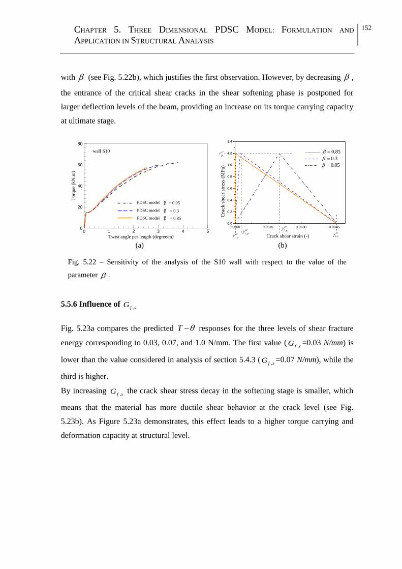
CHAPTER 5. THREE DIMENSIONAL PDSC MODEL: FORMULATION AND
APPLICATION IN STRUCTURAL ANALYSIS
152
with (see Fig. 5.22b), which justifies the first observation. However, by decreasing ,
the entrance of the critical shear cracks in the shear softening phase is postponed for
larger deflection levels of the beam, providing an increase on its torque carrying capacity
at ultimate stage.
(a) (b)
Fig. 5.22 – Sensitivity of the analysis of the S10 wall with respect to the value of the
parameter .
5.5.6 Influence of ,f sG
Fig. 5.23a compares the predicted T responses for the three levels of shear fracture
energy corresponding to 0.03, 0.07, and 1.0 N/mm. The first value (,f sG =0.03 N/mm) is
lower than the value considered in analysis of section 5.4.3 (,f sG =0.07 N/mm), while the
third is higher.
By increasing ,f sG the crack shear stress decay in the softening stage is smaller, which
means that the material has more ductile shear behavior at the crack level (see Fig.
5.23b). As Figure 5.23a demonstrates, this effect leads to a higher torque carrying and
deformation capacity at structural level.
0 1 2 3 4 50
20
40
60
80
wall S10
PDSC model = 0.05
PDSC model = 0.3
PDSC model = 0.85
Torq
ue
(kN
.m)
Twist angle per length (degree/m)
0.0000 0.0015 0.0030 0.00450.0
0.2
0.4
0.6
0.8
1.0
1.2
1.4
0.85
0.3
0.05
cr
p
,
cr
t p,
cr
t p ,
cr
t p
Cra
ck
sh
ear
stre
ss (
MP
a)
Crack shear strain (-) ,u
cr
t

CHAPTER 5. THREE DIMENSIONAL PDSC MODEL: FORMULATION AND
APPLICATION IN STRUCTURAL ANALYSIS
153
(a) (b)
Fig. 5.23 – Sensitivity of the analysis of the S10 wall with respect to the value of the
parameter ,f sG .
5.6 CONCLUSION
This chapter propose a 3D constitutive model for cement based materials, based in the
generalization of a 2D plastic-damage multidirectional fixed smeared crack model. The
proposed model was then included in the 3D solid element of the FEMIX computer code,
and its valdation was executed at the material and structural levels. Cyclic tension-
compression test were simulated at first, followed by sophisticated biaxial and triaxial
tension-compression numerical tests. In these numerical tests the interaction between
cracking and plasticity-damage parts of the model were discussed. It was shown that the
stress-strain predictions of the model for these numerical tests were in a very good
agreement with the solution reported by another author.
A wide range of experimental data from literature including RC column under combined
axial and flexural loading condition, RC beams made by different concrete strength
classes, and RC walls subjected to torsion, are simulated to highlight the capability of the
model to predict with good accuracy the deformation and cracking behaviour of these
types of structures. According to these simulations, the following results can be drawn:
Results of the experimental program executed by El-Maaddawy (2009) reveals
that by increasing length of the eccentricity (e) of the load applied to each column,
the failure load decreases whereas the strains in tensile longitudinal reinforcement
0 1 2 3 4 50
20
40
60
80
cr
Gf,s
wall S10
PDSC model = 1 N/mm
PDSC model = 0.07 N/mmGf,s
PDSC model = 0.03 N/mmGf,s
To
rqu
e(k
N.m
)
Twist angle per length (degree/m)
0.00 0.01 0.02 0.03 0.04 0.05 0.06 0.070.0
0.5
1.0
1.5
N/mm2
N/mm
N/mm
, 1.0f sG
, 0.07f sG
, 0.03f sG
1.2cr
p
Cra
ck
sh
ear
stre
ss (
MP
a)
Crack shear strain (-)
N/mm

CHAPTER 5. THREE DIMENSIONAL PDSC MODEL: FORMULATION AND
APPLICATION IN STRUCTURAL ANALYSIS
154
bars increase. This experimental observation was successfully simulated by the
PDSC model.
In the experimental program of Yang et al. (2003), the primary variable of the test
is the compressive strength of concrete. The specimens are categorized into two
groups: L group which includes the specimens with cf =31.4 MPa, and H group
which includes the specimens having the compressive strength of 78.5 MPa. The
PDSC model was able to simulate with high accuracy the deformational and
cracking behavior of the beams in both groups L and H.
Two walls subjected to torsion loading configuration are simulated by the
proposed model. Predicted torque carrying capacity, ductility, crack pattern for
these walls are in reasonable agreement with the experimental observations.
In this chapter a parametric study is also executed, to acess the sensitivity of the
simulations to the values of the model parameters. In general, for the structure failing in
shear the effect of the model parameters ,f sG ,
,
cr
t p , can be summarized as the
following:
By increasing ,f sG the crack shear stress decay in the softening stage of cr cr
t t
diagram is smaller, which leads to a higher load carrying and deformation
capacity at structural level.
By increasing ,
cr
t p the entrance of the shear cracks in their softening stage is
postponed for larger crack shear deformations, conducting to higher load carrying
and deformation capacity at structural level.
By decreasing the entrance of the critical shear cracks in the shear softening
phase is postponed for larger deflection levels of the beam, providing an increase
on its load carrying capacity at ultimate stage.
For the structures whose failures are governed by inelastic compressive behaviour of the
concrete, the effects of the model parameters cf ,
1c , ,f cG can be summarized as the
following:

CHAPTER 5. THREE DIMENSIONAL PDSC MODEL: FORMULATION AND
APPLICATION IN STRUCTURAL ANALYSIS
155
The higher is the concrete compressive strength (cf ), the higher is the value of
peak stress at c c diagram (i.e.
cf is the stress at peak of c c diagram), and
the larger is the load carrying capacity of the structure.
By increasing 1c the stiffness in the initial force-deflection behaviour of the
structure decreases, but ductility and load carrying capacity at the ultimate stage
of force-deflection behaviour increase.
By increasing ,f cG a more ductile strain softening stage in compression is
simulated, which leads to a higher load carrying and deformation capacity at
structural level.

CHAPTER 5. THREE DIMENSIONAL PDSC MODEL: FORMULATION AND
APPLICATION IN STRUCTURAL ANALYSIS
156

C H A P T E R 6
CONCLUSIONS AND FUTURE PERSPECTIVES
6.1 GENERAL CONCLUSIONS
A two dimensional (2D) constitutive model was developed for predicting the failure
behaviour of structures made by cement based materials when submitted to different
loading paths. The proposed model incorporates a multidirectional fixed smeared crack
approach to simulate crack initiation and propagation, whereas the inelastic behaviour of
material between cracks is treated by a numerical strategy that combines plasticity and
damage theories. The smeared crack model considers the possibility of forming several fixed
cracks in the same integration point during the cracking process. The crack initiation occurs
when the maximum principal tensile stress in an IP attains the concrete tensile strength
under an assumed tolerance. After crack initiation, the relationship between normal stress
and normal strain in the crack coordinate system is simulated via a trilinear or a
quadrilinear diagrams. Two methods are available to simulate the crack shear stress
transfer: one based on the concept of shear retention factor, and the other on a shear
softening diagram that requires some information about fracture mode II propagation.
The plasticity model is formulated in effective stress space and is defined by four entities:
yield function (yield surface); flow rule; evolution law for the hardening variable; and

CHAPTER 6. CONCLUSIONS AND FUTURE PERSPECTIVES 158
condition for defining loading–unloading process. The yield function was derived from
the Willam–Warnke failure criterion, and its evolution during the plastic flow is governed
by a single hardening parameter (for compression). The plasticity part is responsible for
simulating irreversible strains and volumetric strain in compression, whereas the strain
softening and stiffness degradation of the material under compression are simulated in the
framework of continuum damage mechanics, in which the damage is considered as an
isotropic process. In this approach the state of damage in concrete under compression is
equally distributed in all directions, and can be represented by a scalar measure that is
evaluated as a function of the concrete plastic strain.
The model was implemented into the plane stress state element of the FEMIX 4.0
computer program as a new approache to simulate the nonlinear behaviour of concrete
structures. The model is initially validated by simulating stress-strain histories of the
materials loaded on some different scenarios. Monotonic and cyclic uniaxial compressive
tests were simulated at first, followed by a biaxial tension-compression numerical test that
is intended to demonstrate the interaction between cracking and plasticity-damage parts
of the model. The results of the simulated example under uniaxial compressive load
demonstrate the accuracy of the model in capturing the uniaxial behavior of concrete
under compression. Under the cyclic uniaxial compression, the model (nominal stress
response) accurately simulated the stress–strain envelope response registered
experimentally, but overestimates the plastic deformation of the material when unloading
occurs. Under the biaxial tension-compression test the model succeeded to simulate
closing a crack developed in one direction, by imposing compressive load in the
orthogonal direction. The stress-strain prediction of the model for this numerical test was
in a very good agreement with the solution reported by another author.
Subsequently, the model appraisal is performed by simulating experimental tests with
structural reinforced concrete (RC) elements. For this propose, a wide range of
experimental tests was simulated to demonstrate the robustness of the developed model
(two dimensional PDSC model). The numerical simulations have predicted with good
accuracy the load carrying capacity, deformation, crack pattern, and plastic (compressive)
zones of all types of tests analyzed. The results of these analyses demonstrate the

CHAPTER 6. CONCLUSIONS AND FUTURE PERSPECTIVES 159
applicability of the proposed model for simulating structures made by cement based
materials subjected to multi-axial loading configurations.
The previous model (2D-PDSC) was extended in order to be capable of simulating RC
structures modelled by solid finite elements (those where is important to consider a 3D
stress field). This model (3D-PDSC) was implemented in the FEMIX computer code and
its predictive performance was initially validated by executing some numerical tests at the
material level, which were intended as an elementary verification of the basic capabilities
of the model. Next the model appraisal was performed at the structural level.
Experimental tests, from literature, including RC column subjected to different eccentric
loadings, RC beams made by different concrete strength classes, and RC walls subjected
to torsion, are simulated to highlight the capability of the model to predict with good
accuracy the deformation and cracking behaviour of these types of structures. Results of
these analysis indicates the robustness and accuracy of the proposed model for simulating
the structures made by cement based material as subjected to different loading paths.
At the end, a feedback can be presented to the objectives already defined in the
Introduction section (see section 1.2). It can be concluded that all of these objectives are
achieved in this thesis, based on the following justifications: The numerical simulations,
represented in the chapters 3, 4, and 5 shows the proposed models are stable and
numerically effective in the entire loading regime until failure; Experimental tests from
literature, covering a wide range of geometry of specimens, concrete type, loading
configurations, and reinforcement conditions, are simulated to demonstrate the
applicability of the model for simulating the structures subjected to different loading
paths; A parametric study for the model parameters is executed. Through the parametric
study it was explained how changing each model parameter can affect the predictive
performance of the model; Results of the analysis obtained by the proposed model were
compared also with those of another constitutive model (available in FEMIX) that
includes the same multidirectional fixed smeared crack, to simulate cracking, but
considers the linear elastic behavior for the material between the cracks. In general, and
considering the type of structures analysed, this comparison clearly demonstrated the
advantages of the proposed model for simulating the experimental behaviour of cement

CHAPTER 6. CONCLUSIONS AND FUTURE PERSPECTIVES 160
based material, mainly when relatively large volume of concrete can enter in the
compression softening stage.
6.2 RECOMMENDATIONS FOR FUTURE RESEARCH
6.2.1 Creep model
The constitutive models developed in this study (two and three dimensional PDSC
models), can simulate time dependent irreversible deformations of the material under load
(creep phenomenon). In the current version of the models the incremental concrete strain
vector, co
, (which characterize the deformation of the intact material between the
cracks) is decomposed into its elastic (e
) and plastic parts (p
), (co e p
).
This strain decomposition concept can be extended in order to integrate the parcel due to
creep, crp
, (i.e. co e p crp
). Thereby the incremental constitutive
relation of the new model is obtained as: ( )e p cr crp
D . The
definition of , e
D , , cr
are the same as those introduced in Chapter 3.
Due to this additional term (crp
) the flow rule and isotropically hardening of the yield
surface are remained as before. Stress update process must be augmented by stress
components due to time dependent deformations. Based on the stress update, internal
nodal forces will be calculated and compared by the external one to satisfy the
equilibrium equation.
6.2.2 Numerical simulation of fire condition
Another phenomenon that can be captured by the concept of strain decomposition is the
dependence of the material properties to the temperature. In this way another term of T
related to the thermal variation must be introduced into the constitutive equation of the
plastic-damage multidirectional fixed smeared crack model. Such constitutive equation
can be written as ( )e p cr T
D .
In a previous work (Ventura-Gouveia, 2011) a general thermal model was developed and
introduced in the FEMIX computer code. Steady-state and transient thermal analysis are

CHAPTER 6. CONCLUSIONS AND FUTURE PERSPECTIVES 161
available, including early-age heat generation during the hardening phase of concrete.
Furthermore, the multidirectional fixed 3D smeared crack model was adapted to
incorporate the incremental strain decomposition and a thermo-mechanical model
obtained.
In future developments, the model can be adapted to incorporate the possibility of
simulating structures under high temperatures, like fire condition. A possible application
of the numerical tool can be mentioned in simulating behavior of ECC/FRP panel
strengthening system subjected to the high temperatures. This composite system has been
designed to show considerable residual strength after exposure to fire condition

CHAPTER 6. CONCLUSIONS AND FUTURE PERSPECTIVES 162

REFERENCES
Abrishambaf, A. (2015), “Creep behaviour of cracked steel fibre reinforced self-
compacting concrete laminar structures”, PhD thesis, Department of Civil Engineering,
University of Minho.
Abrishambaf, A., Barros, J.A.O., Cunha, V.M.C.F. (2013), “Relation between fibre
distribution and post-cracking behaviour in steel fibre reinforced self-compacting
concrete panels”, Cement and Concrete Research, 51, 57–66.
Abrishambaf, A., Barros, J.A.O., Cunha, V.M.F.C. (2015), “Tensile stress-crack width
law for steel fibre reinforced self-compacting concrete obtained from indirect (splitting)
tensile tests”, Cement and Concrete Composites, 57, 153–165.
Abu Al-Rub, R.K., Kim, S.M. (2010), “Computational applications of a coupled
plasticity–damage constitutive model for simulating plain concrete fracture”, Engineering
Fracture Mechanics, 77 (10), 1577–1603.
Alfano, G., Crisfield, M.A. (2001), “Finite element interface models for delamination
analysis of laminated composites: mechanical and computational issues”, International
Journal for Numerical Methods in Engineering, 50:1701-1736.
Ayatollahi, M.R., Aliha, M.R.M. (2005), “Cracked Brazilian disc specimen subjected to
mode II deformation”, Engineering Fracture Mechanics, 72, 493-503.
Baghi, H., Barros, J.A.O. (2016), “Shear strengthening of reinforced concrete T beams
with Hybrid Composite Plate”, Composites for Construction Journal, 20 (6).
Ghiassi, B., Marcari, G., Oliveira, D.V., Lourenço, P.B. (2012),” Numerical analysis of
bond behavior between masonry bricks and composite materials”, Engineering Structures,
43, 210-220.
Barros, J.A.O., Dias, S.J.E., Baghi, H., Ventura-Gouveia, A. (2016), “Exploring new
potentialities of NSM CFRP laminates for the shear strengthening of RC beams”, ACI
Structural Journal, 111 (3), 1275-1287.

REFERENCES 164
Barros, J.A.O., Costa, I.G., Ventura-Gouveia, A. (2011), “CFRP flexural and shear
strengthening technique for RC beams: experimental and numerical research”, Advances
in Structural Engineering Journal, 14 (3), 559–81.
Barros, J.A.O., Dias, S. (2013), “Assessment of the effectiveness of the NSM shear
strengthening technique for deep T cross section RC beams”, FRPRCS11, Guimaraes,
Portugal.
Barros, J.A.O., Sena-Cruz, J.M. (2001), “Fracture energy of steel fibre reinforced
concrete“, Journal of Mechanics of Composite Materials and Structures, 8 (1), 29-45.
Barros, J.A.O., Varma, R.K., Sena-Cruz, J.M., Azevedo, A.F.M. (2008), “Near surface
mounted CFRP strips for the flexural strengthening of RC columns - experimental and
numerical research”, Engineering Structures Journal, 30 (12), 3412-3425.
Bazant, Z.P., Oh, B.H. (1983), “Crack band theory for fracture of concrete”, Materials
and Structures, 16 (3), 155-177.
Bazant, Z.P., Caner, F.C., Carol, I., Adley, M.D., Akers, S.A. (2000), “Microplane model
M4 for concrete: I Formulation with work-conjugate deviatoric stress”, Journal of
Engineering Mechanics, 126 (9), 944-953.
Camacho, G.T., Ortiz M. (1996), “Computational modeling of impact damage in brittle
materials”, International Journal of Solids and Structures, 33, 2899-2938.
Carrazedo, R., Mirmiran, A., Hanai, J.B. (2013), “Plasticity based stress–strain model for
concrete confinement”, Engineering Structures, 48, 645–657.
Carol, I., Rizzi, E., William, K.J. (2001), “On the formulation of anisotropic elastic
degradation.: II. Generalized pseudo-Rankine model for tensile damage”, International
Journal Solids and Structures, 38, 519–46.
CEB-FIP. Model Code 2010 (2010), Tomas Telford, Lausanne, Switzerland.
Cervenka, J., Papanikolaou, V. (2008), “Three dimensional combined fracture–plastic
material model for concrete”, International Journal of Plasticity, 24:2192–2220.

REFERENCES 165
Cerfontaine, B., Dieudonné, A.C., Radu, J.P., Collin, F., Charlier, R. (2015), “3D zero-
thickness coupled interface finite element: Formulation and application”, Computers and
Geotechnics, 69, 124-140.
Cervenka, J., Bažant, Z.P., Wierer, M. (2005), “Equivalent localization element for crack
band approach to mesh sensitivity in microplane model”, International Journal for
Numerical Methods in Engineering, 62 (5), 700–726.
Chen, W.F., Han, D.J., (1988), “Plasticity for structural engineers”, Springer, New York.
Cicekli, U., Voyiadjis, G.Z., Abu Al-Rub R.K. (2007), “A plastic and anisotropic damage
model for plain concrete”, International Journal of Plasticity, 23, 1874–900.
Coutinho, A.L.G.A., Martins, M.A.D., Sydenstricker, R.M., Alves, J.L.D., Landau, L.
(2003), “Simple zero thickness kinematically consistent interface elements”, Computers
and Geotechnics, 30 (5), 347–374.
Cunha, V.M.C.F. (2010), “Steel fibre reinforced self-compacting concrete-from
micromechanics to composite behaviour”, University of Minho, Guimaraes, Portugal,
(PhD thesis).
Cunha, V.M.C.F., Barros, J.A.O., Sena-Cruz, J.M. (2012), “A finite element model with
discrete embedded elements for fibre reinforced composites”, Computers and Structures,
94-95, 22-33.
de Borst, R., Remmers, J.J.C., Needleman, A., Abellan, M. A. (2004), “Discrete vs
smeared crack models for concrete fracture: bridging the gap”, International Journal for
Numerical and Analytical Methods in Geomechanics, 28, 583-607.
de Borst, R., Nauta, P. (1985), “Non-orthogonal cracks in a smeared finite element
model”, Engineering Computations, 2, 35-46.
de Borst, R. (1986), “Computational aspects of smeared crack analysis”, In: Hinton, E.,
Owen, D.R.J. (Eds.), Computational Modelling of Reinforced Concrete. Pineridge Press,
Swansea, 44–83.
Dias-da-Costa, D.A.S.G. (2010), “Strong discontinuities in the scope of the discrete crack
approach”, PhD thesis, Department of Civil Engineering, University of Coimbra.
REFERENCES 166
Dunne, F., Petrinic, N. (2005), “Introduction to computational plasticity”, Oxford
University Press.
Edalat-Behbahani, A., Barros, J.A.O., Ventura-Gouveia, A. (2015), “Plastic-damage
smeared crack model to simulate the behaviour of structures made by cement based
materials”, International Journal of Solids Structures, 73-74, 20-40.
Edalat-Behbahani, A., Barros, J.A.O., Ventura-Gouveia, A. (2016), “Application of
plastic-damage multidirectional fixed smeared crack model in analysis of RC structures”,
Engineering Structures, 125, 374-391.
El-Maaddawy, T. (2009), “Strengthening of eccentrically loaded reinforced concrete
columns with fiber-reinforced polymer wrapping system: experimental investigation and
analytical modeling”, Journal of Composites for Construction, 13 (1), 13-24.
El-Maaddawy, T.A, Sherif, S. (2009), “FRP composites for shear strengthening of
reinforced concrete deep beams with openings”, Composite Structures, 89, 60–69.
Faria, R. Oliver, J. Cervera, M. (1998), “A strain-based plastic viscous-damage model for
massive concrete structures”, International Journal Solids and Structures, 35 (14), 1533-
1558.
Feenstra, P.H. (1993), “Computational aspect of biaxial stress in plain and reinforced
concrete” PhD thesis, Department of Civil Engineering, Delft University of Technology.
Feenstra, P.H., de Borst, R. (1996), “A composite plasticity model for concrete”,
International Journal of Solids and Structures, 33 (5), 707-730.
Ferrara, L., di Prisco, M. (2001), “Mode I fracture behavior in concrete: nonlocal damage
modeling”, Journal of Engineering Mechanics, 127 (7), 678-692.
Gernay, T. (2012), “A multiaxial constitutive model for concrete in the fire situation
including transient creep and cooling down phases”, PhD Thesis, University of Liege,
Belgium.

REFERENCES 167
Gernay, T., Millard, A., Franssen, J. (2013), “A multiaxial constitutive model for concrete
in the fire situation: Theoretical formulation”, International Journal of Solids Structures,
50, 3659-3673.
Grassl, P., Jirasek, M. (2006), “Damage–plastic model for concrete failure”, International
Journal of Solids and Structures, 43, 7166–7196.
Grassl, P., Lundgren, K., Gylltoft. K. (2002), “Concrete in compression: a plasticity
theory with a novel hardening law”, International Journal of Solids and Structures, 39,
5205–5223.
Grassl, P., Xenos, D., Nystrom, U., Rempling, R., Gylltoft, K. (2013), “CDPM2: A
damage-plasticity approach to modelling the failure of concrete”, International Journal of
Solids and Structures, 50, 3805–3816.
Hansen, E., William, K., Carol, I. (2001), “A two-surface anisotropic damage/plasticity
model for plain concrete”, In: de Borst R., Mazars J., Pijaudier-Cabot G., van Mier
J.G.M., editors. Fracture mechanics of concrete structures, Lisse: Balkema, 549–556.
Hassan, A.M.T., Jones, S.W., Mahmud, G.H. (2012), “Experimental test methods to
determine the uniaxial tensile and compressive behaviour of ultra high performance fibre
reinforced concrete (UHPFRC)”, Construction and Building Materials, 37, 874–882.
Hawileh, R.A. (2012), “Nonlinear finite element modeling of RC beams strengthened
with NSM FRP rods”, Construction and Building Materials, 27, 461–471.
Hawileh, R.A, El-Maaddawy, T.A, Naser, M.Z. (2012), “Nonlinear finite element
modelling of concrete deep beams with openings strengthened with externally-bonded
composites”, Materials and Design, 42, 378-387.
Hillerborg, A., Modéer, M., Petersson, P.E. (1976), “Analysis of crack formation and
crack growth in concrete by means of fracture mechanics and finite elements”, Cement
and Concrete Research, 6 (6), 773-781.
Hisabe, N., Yoshitake, I., Tanaka, H., Hamada, S. (2006), “Mechanical behaviour of fiber
reinforced concrete element subjected to pure shearing stress”, International RILEM

REFERENCES 168
workshop on high performance finer reinforced cementitious composites in structural
applications, RILEM Publication SARL, 375-381.
Hugues, B.P., Chapman, G.P. (1966), “The deformation of concrete and micro-concrete
in compression and tension with particular reference to aggregate size”, Magazine of
Concrete Research, 18 (54), 19-24.
Jason, L., Huerta, A., Pijaudier-Cabot, G., Ghavamian, S. (2006), “An elastic plastic
damage formulation for concrete: Application to elementary tests and comparison with an
isotropic damage model”, Computer Methods in Applied Mechanics and Engineering,
195 (52), 7077-7092.
Jefferson, A.D. (2003), “Craft—a plastic damage contact model for concrete - I. Model
theory and thermodynamic considerations”, International Journal of Solids Structures, 40,
5973-5999.
Jirásek, M. (2004), “Non-local damage mechanics with application to concrete”, RFGC–
8/2004. Failure, Degradation and Instabilities, 683-707.
JSCE-G 553-1999. (2005), “Test method for shear strength of steel fiber reinforced
concrete, Standard specification for concrete structures, Test method and specification”,
JSCE.
Ju, J.W. (1989), “On energy-based coupled elasto-plastic damage theories: constitutive
modeling and computational aspects”, International Journal of Solids and Structures, 25
(7), 803-833.
Kachonov, L.M. (1958), “On the creep fracture time”, Izv. Akad. Nauk USSR Otd. Tech,
8:26–31 [in Russian].
Kaliakin, V.N., Li, J. (1995), “Insight into deficiencies associated with commonly used
zero-thickness interface elements”, Computers and Geotechnics, 17 (2), 225–252.
Karsan, I.D., Jirsa, J.O. (1969), “Behaviour of concrete under compressive loadings”
Journal of Structure Division, ASCE, 95 (12), 2535–2563.

REFERENCES 169
Kim Y.H., Hueste, M.B.D., Trejo, D., Cline, D.B.H. (2010), “Shear characteristics and
design for high strength self-consolidating concrete”, Journal of Structural Engineering,
136 (8), 989-1000.
Kozar, I., Ozbolt, J. (2010), “Some aspects of load-rate sensitivity in visco-elastic
microplane material model”, Computers and Concrete, 7 (4), 317–329.
Krätzig, W.B., Pölling, R. (2004), “An elasto-plastic damage model for reinforced
concrete with minimum number of material parameters”, Computers and Structures, 82
(15-16), 1201-1215.
Kupfer, H., Hilsdorf, H.K., Rusch, H. (1969), “Behaviour of concrete under biaxial states
of stress”, American Concrete Institute journal, 66 (8), 656–666.
Lee, J., Fenves, G.L. (1998), “Plastic-damage model for cyclic loading of concrete
structures”, Journal of Engineering Mechanics Division, ASCE, 124, 892–900.
Lee, J., Fenves, G.L. (2001), “A return-mapping algorithm for plastic-damage models: 3-
D and plane stress formulation”, International Journal of Numerical Methods in
Engineering, 50, 487-506.
Lu, D., Du, X., Wang, G., Zhou, A, Li, A. (2016), “A three-dimensional elastoplastic
constitutive model for concrete”, Computers and Structures, 163, 41-55.
Lubliner, J., Oliver, J., Oller, S., Oñate, E. (1989), “A plastic-damage model for
concrete”, International Journal of Solids and Structures, 25 (3), 299-326.
Luccioni, B.M., Rougier, V.C. (2005), “A plastic damage approach for confined
concrete”, Computers & Structures, 83 (27), 2238-2256.
Maier, J., Thürlimann, B. (1985), “Bruchversuche an Stahlbetonscheiben”, IBK Bericht
8003-1, ETH Zürich, Institut für Baustatik und Konstruktion (IBK), Zürich.
Malvern, L.E., (1969), “Introduction to the mechanics of a continuous medium”,
Prentice-Hall International, Englewood Cliffs, New Jersey.

REFERENCES 170
Marfia, S., Rinaldi, Z., Sacco, E., (2004), “Softening behavior of reinforced concrete
beams under cyclic loading”, International Journal Solids and Structures, 41 (11-12),
3293-3316.
May, S., de Borst, R., Vignollet, J. (2016) “Powell–Sabin B-splines for smeared and
discrete approaches to fracture in quasi-brittle materials”, Computer Methods in Applied
Mechanics and Engineering, 307, 193-214.
Mazaheripour, H., Barros, J.A.O., Sena-Cruz, J.M. (2016), “Tension-stiffening model for
FRC reinforced by hybrid FRP and steel bars”, Composites Part B: Engineering, 88, 162-
181.
Mazars, J., Pijaudier-Cabot, G. (1989), “Continuum damage theory - application to
concrete”. J. Eng. Mech., 115 (2), 345-365.
Meschke, G., Lackner, R., Mang, H.A. (1998), “An anisotropic elastoplastic-damage
model for plain concrete”, International Journal of Numerical Methods in Engineering,
42, 703–727.
Moës, N., Belytschko, T. (2002), “Extended finite element method for cohesive crack
growth”, Engineering Fracture Mechanics, 69 (7), 813-833.
Nechnech, W., Meftah, F., Reynouard, J.M. (2002), “An elasto-plastic damage model for
plain concrete subjected to high temperatures”, Journal of Engineering Structures, 24 (5),
597-611.
Omidi, O., Valliappan, S., Lotfi, V. (2013), “Seismic cracking of concrete gravity dams
by plastic-damage model using different damping mechanisms”, Finite Element in
Analysis and Design, 63, 80-97.
Omidi, O., Lotfi, V. (2013), “Continuum large cracking in a rate-dependent plastic–
damage model for cyclic-loaded concrete structures”, International Journal for Numerical
and Analytical Methods in Geomechanics, 37, 1363–1390.
Oliver, J.A. (1989), “Consistent characteristic length for smeared cracking models”,
International Journal Numerical Methods in Engineering, 28, 461–474.

REFERENCES 171
Oliver, J., Linero, D.L., Huespe, A.E., Manzoli, O.L. (2008), “Two-dimensional
modeling of material failure in reinforced concrete by means of a continuum strong
discontinuity approach”, Computer Methods in Applied Mechanics and Engineering, 197,
332-348.
Ortiz, M. (1985), “A constitutive theory for inelastic behaviour of concrete”, Mechanics
of Materials, 4, 67–93.
Ortiz, M., Pandolfi, A. (1999), “Finite-deformation irreversible cohesive elements for
three-dimensional crack-propagation analysis, International Journal for Numerical
Methods in Engineering, 44, 1267-1282.
Papanikolaou, V.K., Kappos, A.J. (2007), “Confinement-sensitive plasticity constitutive
model for concrete in triaxial compression”, International Journal of Solids and
Structures, 44 (21), 7021–7048.
Park, H., Kim, J.Y. (2005), “Plasticity model using multiple failure criteria for concrete in
compression”, International Journal of Solids and Structures, 42 (8), 2303-2322, 2005.
Pereira, E.B. (2012), “Processes of cracking in strain hardening in cementitious
composites”, PhD Thesis, University of Minho, Portugal.
Petrova,V.E., Sadowski, T. (2012), “Theoretical analysis of Mode II cracks in a compact
shear specimen”, Computational Materials Science, 64, 248-252.
Poltronieri, F., Piccolroaz, A., Bigoni, D., Romero Baivier, S. (2014), “A simple and
robust elastoplastic constitutive model for concrete”, Engineering Structures, 60, 81–84.
Peng, X.N., Wong, Y.L. (2011), “Behavior of reinforced concrete walls subjected to
monotonic pure torsion-an experimental study”, Engineering structures, 33, 2495-2508.
Reinhardt, H.W. (1984), “Fracture mechanics of an elastic softening material like
concrete”, Heron, 29 (2), 1-42.
Ristinmaa, M., Wallin, M., Ottosen, N.S. (2007), “Termodynamic format and heat
generation of isotropic hardening plasticity”, Acta Mechanica.

REFERENCES 172
Rao, G.A., Rao, A.S. (2009), “Toughness indices of steel fiber reinforced concrete under
mode II loading”, Materials and Structures, 42, 1173–1184.
Rots, G.J., de Borst, R. (1987), “Analysis of mixed mode fracture in concrete”, Journal of
Engineering Mechanics, 113 (11), 1739-1758.
Rots, J.G. (1988), “Computational modeling of concrete structures”, PhD Thesis, Delft
University of Technology.
Sagaseta, J., Vollum, R.L. (2011), “Shear design of short-span beams”. Magazine of
Concrete Research, 62, 4, 267-282.
Schellekens, J.C.J. (1990), Interface elements in finite element analysis”, Report25.2-90-
2-17, Delft University of Technology, Delft.
Seguarado, J., LLorca, J. (2004), “A new three-dimensional interface finite element to
simulate fracture in composites”, International Journal of Solids and Structures, 41:2977-
2993.
Sena-Cruz, J.M. (2004), “Strengthening of concrete structures with near-surface mounted
CFRP laminate strips”, PhD thesis, Department of Civil Engineering, University of
Minho.
Sena-Cruz, J.M., Barros, J.A.O., Azevedo, A.F.M., Ventura-Gouveia, A. (2007),
“Numerical simulation of the nonlinear behaviour of RC beams strengthened with NSM
CFRP strips”, Proceedings of CMNE/CILAMCE Congress, FEUP, Porto, Portugal.
Soltanzadeh, F., Edalat-Behbahani, A., Mazaheripour, H., Barros, J.A.O. (2016a) “Shear
resistance of SFRSCC short-span beams without transversal reinforcements, Composites
Structures, 139, 42-61.
Soltanzadeh, F., Edalat-Behbahani, A., Barros, J.A.O., Mazaheripour, H. (2016b), “Effect
of fiber dosage and prestress level on shear behavior of hybrid GFRP-steel reinforced
concrete I-shape beams without stirrups”, Composites Part B: Engineering, 102, 57-77.
Simone, A. (2007), “Continuous-discontinuous modelling of failure”, Rev Eur Génie
Civil, 11(7–8), 1069–1085, http://dx.doi.org/10.1080/17747120.2007.9692977.

REFERENCES 173
Simo, J.C., Hughes, T.J.R. (1998), “Computational inelasticity”, Springer.
Sinha, B.P., Gerstle, K.H., Tulin, L.G. (1964), “Stress-strain relations for concrete under
uniaxial loading”, ACI Structural Journal, 61(2), 195-211.
Schellekens, J.C.J., de Borst, R. (1993), “On the numerical integration of interface
elements”, International Journal for Numerical Methods in Engineering, 36 (1), 43–66.
Shah, S.P., Swartz, S.E., Ouyang, C. (1995), “Fracture Mechanics of Concrete:
Applications of Fracture Mechanics to Concrete, Rock and Other Quasi-Brittle
Materials”, John Wiley & Sons, Inc.
Suidan, M., Schnobrich, W.C. (1973), “Finite element analysis of reinforced concrete”,
Journal of Structural Division, ASCE, 99 (10), 2109-2122.
Suryanto B., Nagai K, Maekawa K. (2010), “Modeling and analysis of shear-critical ECC
members with anisotropic stress and strain fields”, Journal of Advanced Concrete
Technology, 8 (2), 239–258.
Swaddiwudhipong, S., Seow, P.E.C. (2006), “Modelling of steel fiber-reinforced concrete
under multi-axial loads”, Cement and Concrete Research, 36, 1354–1361.
Tao, X., Phillips, D.V. (2005), “A simplified isotropic damage model for concrete under
bi-axial stress states”, Cement and Concrete Composites, 27 (6), 716-726.
Taqieddin, Z.N. (2008) “Elasto-plastic and damage modelling of reinforced concrete”,
PhD thesis, Department of Civil and Environmental Engineering, Louisiana State
University.
Taqieddin, Z., Voyiadjis, G.Z., Almasri, A.H. (2012), “Formulation and verification of a
concrete model with strong coupling between isotropic damage and elastoplasticity and
comparison to a weak coupling model”, Journal of Engineering Mechanics ASCE, 138,
530–541.
Thanoon, W.A., Alwathaf, A.H., Noorzaei, J., Jaafar, M.S., Abdulkadir, M.R. (2008),
“Nonlinear finite element analysis of grouted and ungrouted hollow interlocking
mortarless block masonry system”, Engineering Structures, 30, 1560-1572.

REFERENCES 174
Tijssens, M.G.A., Sluys B.L.J., Van der Giessen, E. (2000), “Numerical simulation of
quasi-brittle fracture using damaging cohesive surfaces”, European Journal of Mechanics
- A/Solids, 19 (5), 761-779.
Teixeira, M.D.E., Barros, J.A.O., Cunha, V.M.C.F., Moraes-Neto, B.N., Ventura-
Gouveia A. (2015), “Numerical simulation of the punching shear behaviour of self-
compacting fibre reinforced flat slabs” Construction and Building Material, 74, 25-36.
van Mier, J.G.M. (1984), “Strain-softening of concrete under multiaxial loading
conditions”, PhD thesis, Technical University of Eindhoven.
Ventura-Gouveia, A. (2011), “Constitutive models for the material nonlinear analysis of
concrete structures including time dependent effects”, PhD thesis, Department of Civil
Engineering, University of Minho.
Ventura-Gouveia, A., Barros, J.A.O., Azevedo, A.F.M., Sena-Cruz, J.M. (2008),
“Multifixed smeared 3D crack model to simulate the behaviour of fiber reinforced
concrete structures”, Challenges for Civil Construction International Conference
(CCC2008), Porto, Portugal, 16-18.
Vonk, R.A. (1992), “Softening of concrete loaded in compression”, PhD thesis,
Eindhoven University of Technology, The Netherlands.
Voyiadjis, G.Z., Kattan, P.I. (2006), “Advances in Damage Mechanics: Metals and Metal
Matrix Composites, with an Introduction to Fabric Tensors”, Second Edition, Elsevier,
Oxford.
Voyiadjis, G.Z., Taqieddin, Z.N., Kattan, P.I. (2008), “Anisotropic Damage-Plasticity
Model for Concrete”, International Journal of Plasticity, 24 (10), 1946-1965.
Wang, C.H. (1996), “Introduction to fracture mechanics”, DSTO-GD-0103, Airframes
and Engines Division Aeronautical and Maritime Research Laboratory.
Wells, G.N., Sluys, L.J. (2001), “A new method for modelling cohesive cracks using
finite elements”, International Journal of Numerical Methods in Engineering, 50, 2667–
2682.

REFERENCES 175
Willam, K., Rhee, I., Beylkin, G. (2001), “Multiresolution analysis of elastic degradation
in heterogeneous materials”, Meccanica, 36 (1), 131-150.
Willam, K., Rhee, I., Xi, Y. (2003), “Thermal degradation of heterogeneous concrete
materials”, Special issue on Durability, Journal of Materials in Civil Engineering, ASCE,
17 (3), 276-285.
Willam, K.J., Warnke, E.P. (1974), “Constitutive model for the triaxial behaviour of
concrete in Concrete Structures Subjected to Triaxial Stresses.”, volume 19 of IABSE
Report, International Association of Bridge and Structural Engineers, Zurich, 1-30,
Wischers, G. (1978), “Application of Effects of Compressive Loads on Concrete,”
Betontech., Berlin, Nos. 2 and 3, Düsseldorf.
Wu, J.U., Li J., Faria, R. (2006), “An energy release rate-based plastic-damage model for
concrete”, International Journal of Solids and Structures, 43, 583–612.
Wu, H.Q., Gilbert, R.I. (2009), “Modeling short-term tension stiffening in reinforced
concrete prisms using a continuum-based finite element model”, Engineering Structures,
31, 2380-2391.
Xenos, D., Grassl, P. (2016), “Modelling the failure of reinforced concrete with nonlocal
and crack band approaches using the damage-plasticity model CDPM2”, Finite Elements
in Analysis and Design, 117-118, 11-20.
Xu, S., Reinhardt, H.W. (2005), “Shear fracture on the basis of fracture mechanics”, Otto-
Graf Journal, 16, 21-78.
Yang, K.H., Chung, H.S., Lee, E.T, Eun, H.C. (2003), "Shear characteristics of high-
strength concrete deep beams without shear reinforcements", Engineering Structures, 25,
1343–1352.
Zhang, J., Li, J. (2012), “Investigation into Lubliner yield criterion of concrete for 3D
simulation”, Engineering Structures, 44, 122–127.

REFERENCES 176
Zhang, J., Li, J., Woody-Ju, J. (2016), “3D elastoplastic damage model for concrete based
on novel decomposition of stress”, International Journal of Solids and Structures, 94-95,
125-137.
Salehian, H., Barros, J.A.O. (2015), “Assessment of the performance of steel fibre
reinforced self-compacting concrete in elevated slabs”, Cement and Concrete
Composites, 55, 268-280.

ANNEX A
GEOMETRIC REPRESENTAION OF STRESS
INVARIANTS
Fig. A.1 represents a three dimensional orthogonal coordinate system aligned in the
directions of the principal stresses (1 ,
2 , 3 ), which is known as Haigh- Westergaard
coordinate system. An additional axis, called Hydrostatic axis, is also defined in this
figure, which is aligned in the direction of the bisector 1 2 3 . The state of stress for
every point on the hydrostatic axis is 1 2 3 . Any plane perpendicular to
Hydrostatic axis is called deviatoric plane.
Consider a generic state of stress represented by point P with the coordinates (1 ,
2 , 3
) in Haigh-Westergaard stress space. Assuming the stress point O is the origin, the stress
vector OP can be decomposed into two components: the component ON in the direction
of hydrostatic axis and the component NP perpendicular to ON (the vector NP is the
projection of OP on the deviatoric plane). The vector NP has the magnitude of
22J , while the magnitude of the vector ON is 1 3I (Chen and Han, 1988).
To trace the exact location of the stress point P in the deviatoric plane, the stress invariant
3J (third invariant of the effective deviatoric stress tensor) is also required. If the triplet
axes 1 ,
2 , 3 are projected on the deviatoric plane, and the axis
1 is taken as the

ANNEX A. GEOMETRIC REPRESENTATION OF STRESS INVARIANTS 178
vertical one, the orientation of the vector NP in the deviatoric plane is defined by the
angle of similarity ( ) according to the following equation (Chen and Han, 1988):
1 3
3/2
2
1 3 3
3 2
Jcos
J
(A.1)
where 2J is second invariant of the effective deviatoric stress tensor.
Fig. A.1 – Haigh-Westergaard stress space (Grassl et al., 2002).
1 2 3
Hydrostatic axis
1 2 3( , , )P
O
N
constant1 2 3
2
3
1
Deviatoric plane

ANNEX B
EXTRACTING YIELD FUNCTION FROM FAILURE
CRITERION
According to the Willam-Warnke failure criterion, two extreme meridians and an
elliptical function, used to interpolate the current failure meridian between the two
extreme meridians, can represent the entire failure surface. The extreme meridians are
called the tensile meridian where angle of similarity is zero ( 0 ), and the compressive
meridian where 60 (see Fig. B.1).
(a) (b)
Fig. B.1 – Willam-Warnke failure surface represented in (a) meridian plane; (b) deviatoric plane (
1 ,2 ,
3 are the principle effective stresses).
/ fc
/f
c
Compressive meridian
Tensile meridian
( 0 < < 60 )Intermediate failure meridian
( = 0 )
( = 60 )
_
_
_
_
_
/ fc
= a0
= b0=c
_
( , 0 )
( , )
( , 60 )
32
1 elliptical curve

ANNEX B. EXTRACTING YIELD FUNCTION FROM FAILURE CRITERION 180
The equations for the tensile and compressive meridians in ( , , ) coordinate system
are given by the following quadratic parabolas (Swaddiwudhipong and Seow, 2006):
2
( , 0 ) ( , 0 )
2 1 0
c c c
a a af f f
2
( , 60 ) ( , 60 )
2 1 0
c c c
b b bf f f
(B.1)
(B.2)
being the hydrostatic stress invariant defined as 1 3I , and the deviatoric stress
invariants also defined as 22 J . The term ( , )
implies the deviatoric stress
invariant ( ) that is corresponds to any set of and . For the tensile meridian (where
0 ) and compressive meridian (where 60 ), the deviatoric stress invariant ( )
are denoted, respectively, by ( , 0 )
and ( , 60 )
.
It is assumed that the tensile and compressive parabolas (meridians) intersect each other
at the hydrostatic axis, 22 J =0, therefore 0 0a b (Willam and Warnke, 1974;
Swaddiwudhipong and Seow, 2006).
The constants 0a ,
1a , 2a ,
1b , and 2b are the five constants of the W-W failure surface, and
the procedure used in their determination is discussed in the following. To obtain the
unknowns 0a ,
1a , 2a (which are the coefficients of the tensile meridian) it is sufficient to
choose three known failure states lying on the tensile meridian (Eq. B.1), such that:
1. Uniaxial tensile strength, (ctf ).
2. Biaxial compressive strength, ( 1.15cc cf f ), (Kupfer et al., 1969).
3. An experimental data corresponding to confined biaxial compression with the
coordinate, ( ,c cf f )=(-6.754, 3.461) (Kupfer et al., 1969).

ANNEX B. EXTRACTING YIELD FUNCTION FROM FAILURE CRITERION 181
These three failure points, expressed in ( , , ) coordinate system, are represented in
Table B.1.
Table B.1 – Experimental failure points to determine the constants of tensile meridian
Test Failure points
(cf ) (
cf ) ( )
Uniaxial tension 1
3
ct
c
f
f 2
3
ct
c
f
f
0
Biaxial compression 2(1.15)
3 2
(1.15)3
0
Confined biaxial compression -6.754
3.461 0
Including these three failure point, represented in Table B.1, into Eq. (B.1), yields after
some arrangement the following system of equations:
2
0
2
1
2 2
2 2 11
3 3 3
2 2 21 1.15 (1.15) (1.15)
3 3 3
1 3.461 (3.461) 6.754
a
a
a
(B.3)
being a non-dimensional parameter defined as ct cf f . According to the approach
adopted in the PDSC model, the tensile crack opening is initiated based on the Rankine
tensile criterion (i.e. a crack occurs when the maximum principal tensile stress in a IP
attains ctf ), so the plasticity part does not required to account for the tensile cracking
behavior of concrete. Therefore to determine the parameter for the plasticity model,
the value of concrete tensile strength, ctf , was replaced by
cf (i.e. 1c cf f ), which
is a higher value adopted to prevent the crack opening based on the plasticity failure
criterion.
The coefficients of the tensile meridian (0a ,
1a ,2a ), which are the unknowns of the
equation B.3, can be deduced as:

ANNEX B. EXTRACTING YIELD FUNCTION FROM FAILURE CRITERION 182
2
0 2
3(7.4241 0.6737 )
8.197 9.0605 1.6814a
(B.4a)
2
1 2
3( 5.7392 3.694 2.091 )
8.197 9.0605 1.6814a
(B.4b)
2 2
3( 1.0098 3.3911 )
8.197 9.0605 1.6814a
(B.4c)
The same procedure is repeated for the unknown coefficients of the compressive
meridians (b1, b2). Two failure states (failure points) lying on the compressive meridian (
60 ) are used as:
1. Uniaxial compressive strength, (cf ), ( ,c cf f )=( 1 3 , 2 3 ).
2. An experimental data corresponding to confined biaxial compression with the
coordinate, ( ,c cf f )=(-3.3774, 2.77), (Kupfer et al., 1969).
By substituting the coordinates of these two failure points into equation of compressive
meridian (Eq. B.2), the following system of equations is obtained:
1 0
22 0
2 2( 1 3)
3 33.3774
2.77 (2.77)
b b
b b
(B.5)
By taking into account 0b =
0a , the coefficients 1b and
2b are obtained by solving Eq. (B.5).
These coefficients in the final form are as the following:
2
1 2
3( 2.3328 9.169 1.5469 )
8.197 9.0605 1.6814b
(B.6d)

ANNEX B. EXTRACTING YIELD FUNCTION FROM FAILURE CRITERION 183
2
2 2
3( 1.2437 4.6489 0.04254 )
8.197 9.0605 1.6814b
(B.6e)
The W-W failure criterion uses the following elliptical equation to interpolate current
failure meridian, or the intermediate failure meridians, between the two extremes (tensile
and compressive meridians) (Willam and Warnke, 1974; Swaddiwudhipong and Seow,
2006):
( , )
s
t
(B.7a)
where
2 2
( , 60 ) ( , 60 ) ( , 0 ) ( , 60 ) ( , 0 ) ( , 60 )
1/22 2 2 2
( , 60 ) ( , 0 ) ( , 0 ) ( , 0 ) ( , 60 )
2 ( )cos (2 )
4( )cos 5 4
s
(B.7b)
and
2 2 2 2
( , 60 ) ( , 0 ) ( , 60 ) ( , 0 )4( )cos ( 2 )t
(B.7c)
being ( , )
is the deviatoric stress invariant of current failure meridian (see Fig. B.1b that
demonstrates the deviatoric plane of W-W). As Fig. B.1b shows, Eq. (B.7) ensures
convexity and smoothness of the surface anywhere. Eqs. (B.1), (B.2) and (B.7) describe
one sixth of the failure cone lying between 0 60 , then due to six fold symmetry,
these equations are sufficient to present the entire failure surface.
The intermediate failure meridians are also quadratic parabola in a form
(Swaddiwudhipong and Seow, 2006):
2
( , ) ( , )
c c c
a b cf f f
(B.8)

ANNEX B. EXTRACTING YIELD FUNCTION FROM FAILURE CRITERION 184
The intermediate meridian must also meet the hydrostatic axis at the same location that
tensile and compressive meridians already intersected, such a requirement implies that
(Swaddiwudhipong and Seow, 2006):
0 0c a b (B.9)
The two unknowns a and b are determined by solving Eq. (B.8) in two known failure
points laying on the intermediate failure meridian. Based on the current state of effective
stress vector ( ) the angle of similarity is calculated from Eq. (A.1) (see Annex A). The
arbitrary control points of cf =
1CP = -0.5 and cf =
2CP = -0.6 can be chosen, then
the corresponding failure points of 1( , )CP
, and 2( , )CP
were interpolated from Eq.
(B.7). The coefficients a and b can then be obtained from:
2
2
( , )
2 0
2
( , )
( ) CP
CP
CP
c
c
a bf
a
f
(B.10)
1 2
2 1 2 1
2 2
( , ) ( , )
2 0 1 0
2
( , ) ( , ) ( , ) ( , )
( ) ( )CP CP
CP CP CP CP
CP CP
c c
c c c c
a af f
b
f f f f
(B.11)
Including 1 3I and
2( , )2 J
into Eq. (B.8) and replacing
cf with the current
uniaxial compressive stress, i.e. the hardening function denoted by c , the equation of
yield function is obtained in the form of Eq. (3.15).
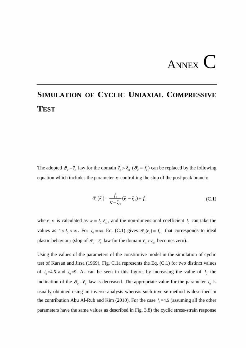
ANNEX C
SIMULATION OF CYCLIC UNIAXIAL COMPRESSIVE
TEST
The adopted c c law for the domain
1c c (c cf ) can be replaced by the following
equation which includes the parameter controlling the slop of the post-peak branch:
1
1
( ) ( )cc c c c c
c
ff
(C.1)
where is calculated as 0 1cl , and the non-dimensional coefficient
0l can take the
values as 01 l . For
0l Eq. (C.1) gives ( )c c cf that corresponds to ideal
plastic behaviour (slop of c c law for the domain
1c c becomes zero).
Using the values of the parameters of the constitutive model in the simulation of cyclic
test of Karsan and Jirsa (1969), Fig. C.1a represents the Eq. (C.1) for two distinct values
of 0l =4.5 and
0l =9. As can be seen in this figure, by increasing the value of 0l the
inclination of the c c law is decreased. The appropriate value for the parameter
0l is
usually obtained using an inverse analysis whereas such inverse method is described in
the contribution Abu Al-Rub and Kim (2010). For the case 0l =4.5 (assuming all the other
parameters have the same values as described in Fig. 3.8) the cyclic stress-strain response

ANNEX C. SIMULATION OF CYCLIC UNIAXIAL COMPRESSIVE TEST 186
of the model for the test of Karsan and Jirsa (1969) is represented in Fig. C.1b which
demonstrates a close approximation of the residual plastic deformations when compared
to those registered in the experimental test.
(a) (b)
Fig. C.1 – Cyclic uniaxial compressive test of Karsan and Jirsa (1969) ; (a) the c c law of the
model, (b) Experimental (Karsan and Jirsa, 1969) vs. predicted stress-strain response (assuming 0l
=4.5).
Eq. (3.20)
(C.1)
(C.1)
0 0.001 0.002 0.003 0.004 0.0050
5
10
15
20
25
30
35
40
45
50
Experimental results
PDSC model (nominal stress space)
PDSC model (effective stress space)
Axial strain (-1)
Ax
ial
stre
ss(M
Pa)
(1-dC)E
E

ANNEX D
FIRST AND SECOND ORDER DERIVATIVES
D.1 Derivative of the stress invariants with respect to the components of the effective
stress vector
For a general case of three dimensional problem, the effective stress tensor is written in
the vector format as:
T
i j x y z yz xz xy (D.1)
The first order derivatives of the stress invariants 1I ,
2J , and 3J with respect to
components of the effective stress vector (i ) are defined as the following:
1 1 1 1 1 11; 0x y z yz xz xy
I I I I I I
(D.2)

ANNEX D. FIRST AND SECOND ORDER DERIVATIVES 188
2 2
2 2
2 2
12 , 2
3
12 , 2
3
12 , 2
3
x y z yz
x yz
y x z xz
y xz
z x y xy
z xy
J J
J J
J J
(D.3a)
(D.3b)
(D.3c)
2 2 23
2 2 2
2 2 23
2 2 2
2 2 23
2 2 2
12 2 2 4
9
12
3
12 2 2 4
9
12
3
12 2 2 4
9
12
3
x y z x y x z y z
x
xy xz yz
y x z x y y z x z
y
xy yz xz
z x y x z y z x y
z
xz yz xy
J
J
J
(D.4a)
(D.4b)
(D.4c)
3
3
3
22 2
3
22 2
3
22 2
3
yz y z x xy xz
yz
xz x z y xy yz
xz
xy x y z xz yz
xy
J
J
J
(D.4d)
(D.4e)
(D.4f)
D.2 Derivative of the yield function with respect to the components of the effective
stress vector
The first order derivative of the yield function with respect to the components of the
effective stress vector (i ) is given by:

ANNEX D. FIRST AND SECOND ORDER DERIVATIVES 189
1
2
12 2
0.51 22 2
22
; ( ) 1 2 2
2 3
1 2 1
23
2( )
c c
c
i
c
i i i
i i
f I b aJ J
c cc
I JbJ J b
cc
JaJ a
c
(D.5)
D.3 Derivative of the coefficients of loading meridian (a, b) with respect to the
components of stress vector
First order derivatives of the coefficient of the loading meridian parabola (coefficients a,
and b) with respect to the components of the effective stress vector (i ), are as follows:
2 1
2 1
1 2
2 1 2
1
1 2
( , ) ( , )
1 0 2 0( , ) ( , )
( , ) ( , )1 2 2
( , ) ( , ) ( , )
( , )
( , ) ( , )
2 2
[ 2
2
CP CP
CP CP
CP CP
CP CP CP
CP
CP CP
CP CP
i i i
i i
i
bb b
B B A
2
1
( , )2
( , )]CP
CP
i
(D.6a)
2
2 2
2
2 2
( , ) 2
( , ) ( , )
( , )3
2 0( , ) ( , )2
CP
CP CP
CP
CP CP
i i i
CP
i
a bb
b b
(D.6b)
where the auxiliary variables A and B are defined as:
2 1
2 2
1 0 2 0( , ) ( , )CP CPCP CPA b b
(D.6c)
1 2 2 1
2 2
( , ) ( , ) ( , ) ( , )CP CP CP CPB
(D.6d)

ANNEX D. FIRST AND SECOND ORDER DERIVATIVES 190
It is also noted that according to Eq. (B.9), the constants 0a and
0b have the same value
(i.e. 0 0a b ).
D.4 Derivative of the interpolation function ( , )
(Eq. (B.7a)) with respect to the
components of the effective stress vector
The derivation of the interpolation function respect to the stress vector components (i )
is given by:
( , ) 1
i
D B E A
(D.7a)
0.5
2 2 2 2 2 22 cos 2 4 cos 5 4c c t c t c c t t t cA
(D.7b)
22 2 24 cos 2c t c tB (D.7c)
2 2 24 2 cos sinc t
i
E B
(D.7d)
0.52 2 2 2 2 2
2 2
12 sin 4 cos 5 4
2
2 4 2 cos sin
c c t c t t t c
i
c t c c t
i
D
(D.7e)
where the variables t and c are defined as ( , 0 )t
and ( , 60 )c
,
respectively.
D.5 Derivative of angle of similarity ( ) with respect to the component of the
effective stress vector

ANNEX D. FIRST AND SECOND ORDER DERIVATIVES 191
The angle of similarity is only dependent on the stress field. So, its first order derivation
with respect to the components of the stress vector (i ) is:
3/2 5/23 22 3 2
1 3 3
2 2sin(3 )i i i
J JJ J J
(D.8)
D.6 Derivative of the yield function with respect to the hardening function
First order derivation of the yield function with respect to the hardening function (c ) is
given by:
1/2
1 12 2 2
1 2 2 21
2 3 3c
c
I If b b aJ J J
c c cc
(D.9)
D.7 Second order derivative of stress invariants with respect to the components of
the effective stress vector
The second order derivative of the first invariant of the effective stress tensor, 1I , with
respect to the effective stress components (i ) and (
j ) is given by:
2
1 0j i
I
(D.10)
The second order derivative of of the second invariant of the deviatoric effective stress
tensor, 2J , with respect to the effective stress components (
i ) and (j ) is given by:

ANNEX D. FIRST AND SECOND ORDER DERIVATIVES 192
2 2 2 2 2 2
2 2 2 2
2 1 1; ; ; 0 ; 0 ; 0
3 3 3
1 2 1; ; ;
3 3 3
x x x y x z x yz x xz x xy
y x y y y z y
J J J J J J
J J J J
2 2
2 2 2 2 2 2
2
0 ; 0 ; 0
1 1 2; ; ; 0 ; 0 ; 0
3 3 3
0
yz y xz y xy
z x z y z z z yz z xz z xy
yz x
J J
J J J J J J
J
2 2 2 2 2
2 2 2 2
; 0 ; 0 ; 2 ; 0 ; 0
0 ; 0 ; 0 ; 0 ;
yz y yz z yz yz yz xz yz xy
xz x xz y xz z xz yz xz
J J J J J
J J J J
2 2
2 2 2 2 2 2
2 ; 0
0 ; 0 ; 0 ; 0 ; 0 ; 2
xz xz xy
xy x xy y xy z xy yz xy xz xy xy
J J
J J J J J J
(D.11)
The second order derivative of of the third invariant of the deviatoric effective stress
tensor, 3J , with respect to the effective stress components (
i ) and (j ) is given by:
3 3 3
3 3 3
3
2 2 2(2 ) ; (2 ) ; (2 )
9 9 9
2 2 2(2 ) ; (2 ) ; (2 )
9 9 9
x y z z y x y x z
x x x y x z
z y x y x z x y z
y x y y y z
z x
J J J
J J J
J
3 3
3 3 3
3 3
2 2 2(2 ) ; (2 ); (2 )
9 9 9
4 2 2; ;
3 3 3
2;
3
y x z x y z z y x
z y z z
yz yz yz
yz x yz y yz z
xz
xz x xz y
J J
J J J
J J
3
3 3 3
4 2;
3 3
2 2 4; ;
3 3 3
xz xz
xz z
xy xy xy
xy x xy y xy z
J
J J J
(D.12)

ANNEX D. FIRST AND SECOND ORDER DERIVATIVES 193
3 3 3
3 3 3
3 3
4 2 2; ;
3 3 3
2 4 2; ;
3 3 3
2 2;
3 3
yz xz xy
x yz x xz x xy
yz xz xy
y yz y xz y xy
yz x
z yz z xz
J J J
J J J
J J
3
3 3 3
3 3 3
4;
3
2( 2 ) ; 2 ; 2
3
22 ; ( 2 ) ; 2
3
z xy
z xy
y z x xy xz
yz yz yz xz yz xy
xy x z y yz
xz yz xz xz xz xy
x
J
J J J
J J J
3 3 3 22 ; 2 ; ( 2 )
3xz yz x y z
y yz xy xz xy xy
J J J
D.8 Second order derivative of the yield function with respect to the effective stress
components
The second order derivative of of the yield function with respect to the effective stress
components (i ) and (
j ) is given by:
3/2 1/2; ( ) 1 1
2 2
c c
j i j j
f A BA B A
(D.13a)
where functions A, B and their derivatives (jA ,
jB ) are:
12 2
2 2
3c
I b aA J J
c cc
(D.13b)
0.51 22 2
22
1 2 1
23
2( )
c
i i i
i i
I JbB J J b
cc
JaJ a
c
(D.13c)
1 2 22 2
2
1 2 1 2{ } { }
3 2c
j j j j j j
I J JA b aJ b J a
c cc J
(D.13d)

ANNEX D. FIRST AND SECOND ORDER DERIVATIVES 194
0.5 0.51 22 2
0.5 1.5 0.52 2 2 22 2 2
2 22
1 20.5
3
0.5 0.5
2
j j i j i j i
c
j i i j i j
j i j i j
I JB b bJ J
cc
J J J J bb J J b J
J Ja aJ
c
2
i j i
Jaa
(D.13d)
D.9 Second order derivative of the coefficients of the loading meridian (a, b) with
respect to the effective stress components
The second order derivative of coefficient b with respect to the effective stress
components (i ) and (
j ) is given by:
2 2 2
2
1 1 1
1
2
( , ) ( , ) ( , )
1 0 ( , )
2
( , ) ( , ) ( , )
2 0 ( , )
1 2 2 3
2( ){ }
2( ){ }
2
CP CP CP
CP
CP CP CP
CP
CP
j i j i j i
CP
j i j i
j j
bb
b
B AB B F B G B
2
2 2
1 2 2
2 1
2
1 2
2
2
( , )( 2, ) ( 2, )2
( , ) ( , )
( , ) ( , ) ( , )
( , ) ( , )
( , )
( , ) (
{ 2 }
{2 2
2
CP
CP CP
CP CP CP
CP CP
CP
CP CP
j
j i j i
j i j
i
BA G B A
2 1
1 2 1
2 1
1
1 2
1 2
1
2
( , ) ( , )
, )
( , ) ( , ) ( , )
( , ) ( , )
2
( , )
( , ) ( , )
( , ) ( , ) 2
( , ) (
} 2{
}
{2
CP CP
CP CP CP
CP CP
CP
CP CP
CP CP
CP
j i j
i j i
j i
j i
2
1
2
( , )
, )}CP
CP
j i
(D.14a)
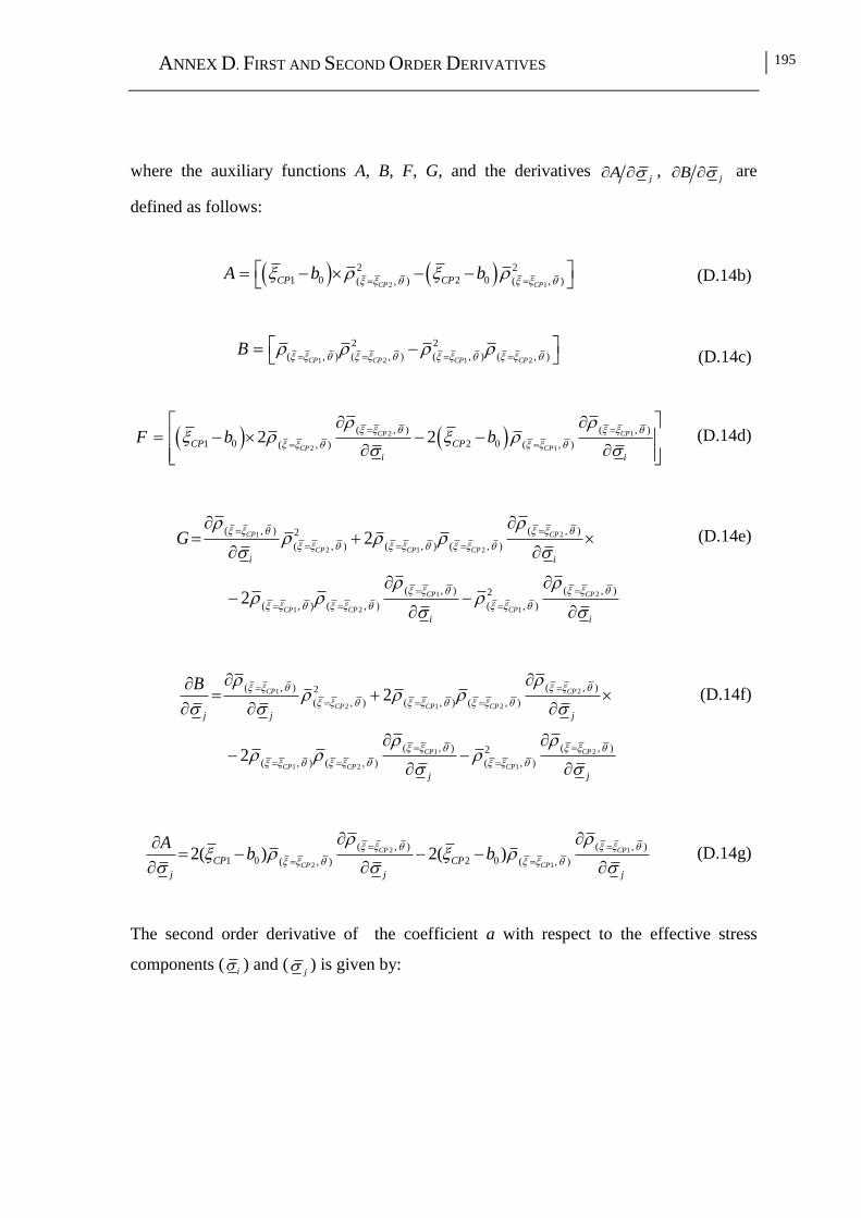
ANNEX D. FIRST AND SECOND ORDER DERIVATIVES 195
where the auxiliary functions A, B, F, G, and the derivatives jA ,
jB are
defined as follows:
2 1
2 2
1 0 2 0( , ) ( , )CP CPCP CPA b b
(D.14b)
1 2 1 2
2 2
( , ) ( , ) ( , ) ( , )CP CP CP CPB
(D.14c)
2 1
2 1
( , ) ( , )
1 0 2 0( , ) ( , )2 2CP CP
CP CPCP CP
i i
F b b
(D.14d)
1 2
2 1 2
1 2
1 2 1
( , ) ( , )2
( , ) ( , ) ( , )
( , ) ( , )2
( , ) ( , ) ( , )
2
2
CP CP
CP CP CP
CP CP
CP CP CP
i i
i i
G
(D.14e)
1 2
2 1 2
1 2
1 2 1
( , ) ( , )2
( , ) ( , ) ( , )
( , ) ( , )2
( , ) ( , ) ( , )
2
2
CP CP
CP CP CP
CP CP
CP CP CP
j j j
j j
B
(D.14f)
2 1
2 1
( , ) ( , )
1 0 2 0( , ) ( , )2( ) 2( )CP CP
CP CPCP CP
j j j
Ab b
(D.14g)
The second order derivative of the coefficient a with respect to the effective stress
components (i ) and (
j ) is given by:

ANNEX D. FIRST AND SECOND ORDER DERIVATIVES 196
2 2
2 2
2 2
2 2
2
2 2( , ) ( , )2
( , ) ( , )
2
( , ) ( , ) 3
( , ) ( , )
( , ) (
2{ }
2 [ 3
CP CP
CP CP
CP CP
CP CP
CP CP
j i j i i j j i
j i i i
j
a b b b
bb b
2 2
2
2
2 2 2
2 2
2 2
, ) ( , ) 4
2 0( , )
2
( , )3
2 0( , ) ( , ) ( , )
( , ) ( , )3
( , ) ( , )
[( )
]] [( )` ]
{ }
CP
CP
CP
CP CP CP
CP CP
CP CP
CP
j i
CP
j i
i j j
b
b b b
bb
(D.15)
D.10 Second order derivative of the interpolation function ( , ) with respect to the
effective stress components
The second order derivative of the interpolation function (( , )
) with respect to the
effective stress components (i ) and (
j ) is given by:
( , )
j i
F G H
.16a)D(
where the auxiliary functions F, G, and H are defined as follows:
22 2 1 2
2 2 2 2
2 {( cos ) ( sin )}
{4 2cos sin } {2 sin }
c c t
j i j i
c t c c t
j i
F B B
.16b)(D

ANNEX D. FIRST AND SECOND ORDER DERIVATIVES 197
2 2 3/2 2 2
1 2
22 1/2 1/2 2
2
1 12 4 2 4 2
2 2
cos ( sin ) ( cos ( sin )) {sin
cos sin cos } {
( sin ) 2 4 cos
c t c c t c t
j i j i
j i j i j
c
G C
B
C B B
2 1/2} cos ( sin )t
i
C
.16c)D(
3 2 2 2 2
2 2 2 2
22 2 2
1/2 2 2
1 { 2 2 4 cos ( sin ) (4 2 ) }
{4 2 (sin cos cos sin
1) } {2 sin (2 )
2
4 4 2 cos ( sin )
c t c t
j
c t
j i j i
c c t c t c
j i j
c t
i
H B D E
B E
C
2 2 2}4 c t B D
.16d)(D
and:
22 2 24 cos 2c t c tB (D.16e)
2 2 2 24 cos 5 4c t t t cC (D.16f)
cos sini
D
(D.16g)
0.5
2 2 2 2 2 22 cos 2 4 cos 5 4c c t c t c c t t t cE (D.16h)

ANNEX D. FIRST AND SECOND ORDER DERIVATIVES 198
where the variables t and
c are defined as ( , 0 )t
and ( , 60 )c
,
respectively.
D.11 Second order derivative of the angle of similarity with respect to the effective
stress components
The second order derivative of the angle of similarity with respect to the effective stress
components (i ) and (
j ) is given by:
3/232
25/2 3/2 5/232 2
3 2 2 2
5/2 7/23 3 2 2 22 2 3
5/
2
33 cot (3 ) cos (3 )
2
31.5
2
1.5 2.5
j i i i
i j i j
i j i j i
Jg ec J
JJ JJ J J J
J J J J JJ J J
J
2
2 33
1
sin(3 )j i
JJ
(D.17)
D.12 Second orderderivative of the yield function with respect to the hardening
function
The second order derivative of the yield function with respect to hardening function (c )
and (c ) is given by:
3/22
1 12 2 2
1 2 2 2
4 3 3c
c c
I If b b aJ J J
c c c
(D.18)
D.13 Second order derivative of the yield function with respect to the hardening
function and to components of stress vector
The second order derivative of the yield function with respect to the hardening function (
c ) and to the components of the effective stress vector (i ) is given by:

ANNEX D. FIRST AND SECOND ORDER DERIVATIVES 199
1/2
12 2
1 22
2
3/2
1 12 2 2
1 22
2
1 2 2
2 3
1 2 1( )
23
1 2 2 2
2 3 3
1 2 1 2( ) (
23
c
i c
i i i
c
i i i
If b aJ J
c c
I Jb bJ
cc J
I Ib a bJ J J
c c c
I Jb b a aJ
c cc J
22 )
i i
JJ a
(D.19)

ANNEX D. FIRST AND SECOND ORDER DERIVATIVES 200

ANNEX E
METHODOLOGY TO DERIVE COMPRESSIVE
FRACTURE ENERGY FROM EXPERIMENTAL DATA
To determine the compressive fracture energy of a generic intervening material, uniaxial
compression test with the set-up like the one represented in Fig. E.1 is recommended.
Fig. E.1 – Set up of uniaxial compression test (Cunha, 2010).
In general, two cones of confined concrete are formed at the top and bottom extremities
of the specimen due to the friction between the steel plates of the test setup and the

ANNEX E. METHODOLOGY TO DERIVE COMPRESSIVE FRACTURE ENERGY FROM
EXPERIMENTAL DATA
202
specimen’s top and bottom ends. The more concrete is confined, in the contact region of
the sample and the steel plates, the higher strength measurement is likely to be. To avoid
the effect of confinement on the measured strength of the specimens the following
treatments are recommended:
- Application of intermediate layers of teflon between the specimen’s top and
bottom ends and the steel plates to reduce the friction between the two surfaces.
- If a cylinder specimen is adopted, the height of the specimen should be higher
than, at least, two times of the cylinder diameter. Only the central region of the
cylinder specimen is monitored, since the state of stress in this region is more
likely to be uniaxial (i.e. the confined concrete cones at the top and bottom
extremities have minimum effect on the state of stress in the central region of the
specimen).
As can be seen in Fig. E.1, the two ring devices were positioned at top and bottom of the
central region of the specimen (here is called “test region”). The axial displacement of the
specimen at the “test region”, s , was measured using three linear voltage displacement
transducers, LVDTs, placed in such a way as depicted in Fig. E.1.
Considering denotes stress measured at the test, the compressive fracture energy can
be determined by the area under the post-peak branch of inel diagram, see Fig. E.2
(Jansen and Shah 1997; Vasconcelos et al., 2009). Inelastic displacement, inel , is
calculated from the following equation:
0
inel sk
(E.1)
where k0 is the initial stiffness of inel response (see Fig. E.2).

ANNEX E. METHODOLOGY TO DERIVE COMPRESSIVE FRACTURE ENERGY FROM
EXPERIMENTAL DATA
203
Fig. E.2 – Model for determination of inel .
cf
S
inel
0k0k 0k