conflict risk indicators: significance and data management...
TRANSCRIPT

Matina Halkia
Stefano Ferri
Inès Joubert-Boitat
Francesca Saporiti
Conflict Risk Indicators: Significance and Data Management in the GCRI
2017
EUR 28860 EN
This publication is a Technical report by the Joint Research Centre (JRC), the European Commission’s science
and knowledge service. It aims to provide evidence-based scientific support to the European policymaking
process. The scientific output expressed does not imply a policy position of the European Commission. Neither
the European Commission nor any person acting on behalf of the Commission is responsible for the use that
might be made of this publication.
Contact information
Name: Matina Halkia
Address: Joint Research Centre, Via Enrico Fermi 2749, TP 480, 21027 Ispra (VA), Italy
Email: [email protected]
Tel.: +39 0332786242
JRC Science Hub
https://ec.europa.eu/jrc
JRC107996
EUR 28860 EN
PDF ISBN 978-92-79-75768-6 ISSN 1831-9424 doi:10.2760/44005
Luxembourg: Publications Office of the European Union, 2017
© European Union, 2017
Reuse is authorised provided the source is acknowledged. The reuse policy of European Commission documents
is regulated by Decision 2011/833/EU (OJ L 330, 14.12.2011, p. 39).
For any use or reproduction of photos or other material that is not under the EU copyright, permission must be
sought directly from the copyright holders.
How to cite this report: Halkia, S., Ferri, S., Joubert-Boitat, I., Saporiti, F., Conflict Risk Indicators:
Significance and Data Management in the GCRI, EUR 28860 EN, Publications Office of the European Union,
Luxembourg, 2017, ISBN 978-92-79-75768-6, doi:10.2760/44005, JRC107996.
All images © European Union 2017, except: Cover Image, Photo taken during the 72hr ceasefire between
Hamas and Israel on 6th of August 2014. Destroyed ambulance in Shuja'iyya in the Gaza Strip, Boris Niehaus
(www.1just.de)www.1just.de, 6 August 2014, 17:49:24. Source:
https://commons.wikimedia.org/wiki/File:Destroyed_ambulance_in_the_CIty_of_Shijaiyah_in_the_Gaza_Strip.
jpg

Conflict Risk Indicators: Significance and Data Management in the GCRI

1

Table of contents
Abstract ............................................................................................................... 1
1. Introduction ................................................................................................. 2
2. Data Management ......................................................................................... 3
3. Variable definition ....................................................................................... 11
3.1. Regime Type (REG_U) .......................................................................... 11
3.2. Lack of Democracy (REG_P2) ................................................................ 15
3.3. Government effectiveness (GOV_EFF) .................................................... 17
3.4. Level of repression (REPRESS)............................................................... 18
3.5. Empowerment rights (EMPOWER) .......................................................... 20
3.6. Recent Internal Conflict (CON_INT) ........................................................ 22
3.7. Neighbouring Conflict (CON_NB) ............................................................ 26
3.8. Years Since Highly Violent Conflict (YRS_HVC) ......................................... 28
3.9. Corruption (CORRUPT) .......................................................................... 30
3.10. Ethnic Power Change (ETHNIC_NP) ........................................................ 32
3.11. Ethnic Compilation (ETHNIC_SN) ........................................................... 38
3.12. Transnational Ethnic Bonds (DISPER) ..................................................... 40
3.13. Homicide Rate (HOMIC) ........................................................................ 42
3.14. Infant Mortality (MORT) ........................................................................ 44
3.15. GDP Per capita (GDP) ........................................................................... 45
3.16. Income Inequality (INEQ_SWIID) .......................................................... 47
3.17. Openness (ECON_ISO) ......................................................................... 49
3.18. Food Security (FOOD)........................................................................... 53
3.19. Unemployment (UNEMP) ....................................................................... 59
3.20. Water Stress (WATER) .......................................................................... 60
3.21. Oil Producer (FUEL_EXP) ....................................................................... 62
3.22. Structural Constraints (STRUCT) ............................................................ 63
3.23. Population Size (POP) ........................................................................... 65
3.24. Youth Bulge (YOUTHBBOTH) ................................................................. 67

4. Composite Model ........................................................................................ 71
4.1. Model description ................................................................................. 71
4.2. Model results ....................................................................................... 74
5. Conclusion ................................................................................................. 76
6. References ................................................................................................. 77
7. List of figures ............................................................................................. 79
8. List of tables .............................................................................................. 80

1
Abstract
This technical report presents the composite model of the Global Conflict Risk Index, used
to give an insight into the contributing factors of conflict at country level. This release
features the data sources, the characteristics of the data, the model computing it and the
results, with the objective of improving the documentation on the variables and on the
composite model.
A reliable data management system is presented, which combines the data from various
sources and imputes missing data. Specific statistical methods (numerical classification,
imputation, linear and log rescaling and arithmetic mean) are then used so as to obtain
the final index score for each country since 2006, integrated in country profiles.
While the focus is on presenting the current composite model, as well as the optimization
effort which took place during the course of 2017, the present report also touches on the
potential for improvements with regard to specific aspects of the model input and the
running of the model.
This document focuses on the variables included in the GCRI and their influences on the
composite model. For details regarding the theoretical framework, please see the previous
scientific reports, doi 10.2788/184 and doi 10.2788/705817.

2
1. Introduction
The Global Conflict Risk Index (GCRI) is an early warning system designed to give policy
makers a global risk assessment based on economic, social, environmental, security and
political factors.
Previous versions of the GCRI have incrementally developed a statistical regression
methodology for defining conflict. The composite model was developed for providing an
overview on the factors contributing to conflict. Based on literature review from the conflict
science field, five theoretical risk areas were identified (see risk assessment factors
above). Within these, a further distinction was made between concepts, which were then
represented with individual variables. The variables used are all relatively stable, in that
little change is to be expected from year to year. The risk-of-conflict is assessed by the
composite model at country level based on these variables. It consists in computing raw
data for creating each of the variables, and in compiling all of them into one final score
(per country). Country profiles are finally produced, in which the composite model’s results
are visualized, namely the final score of conflict risk and the background data used to
calculate it using the variables.
This report presents the work done between February 2017 and September 2017, which
has focused on quality control of the dataset, and on improving the documentation of the
composite model. While the work presented here shows great advances in reliability and
reproducibility, there is still potential for improvements.
The report is structured to present the three main aspects of the GCRI composite model:
the data management, the variables and the model. While the first part gives an overview
on the variables and the datasets used, each indicator used for all the variables is
described in detail in the second part, including a general description, its relevance with
regard to conflict risk, where the data is sourced and how the data is transformed. In the
third part, the composite model is described and the results are presented through specific
examples.
3
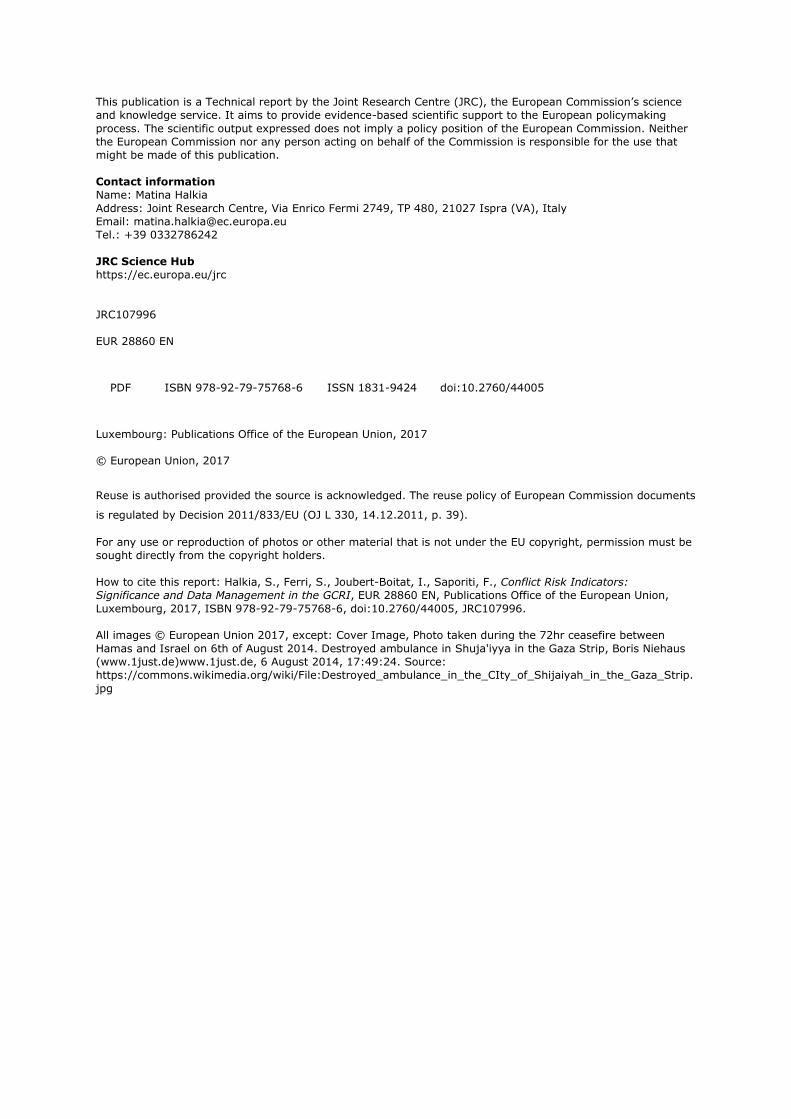
2. Data Management
This section is meant to provide all the necessary information for the user on the data
management.
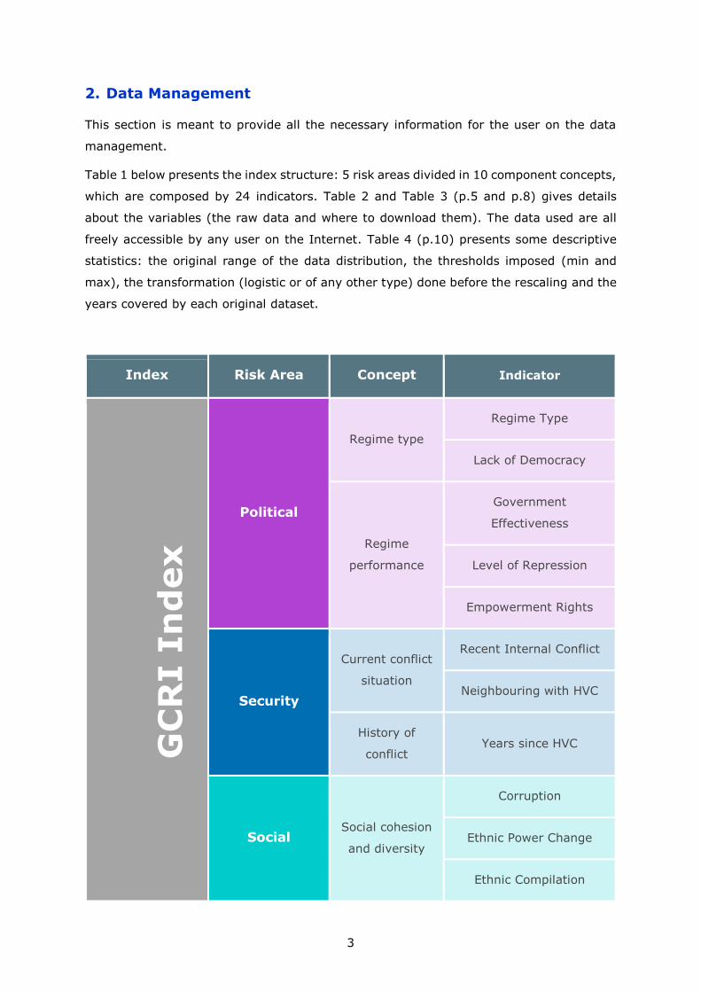
Table 1 below presents the index structure: 5 risk areas divided in 10 component concepts,
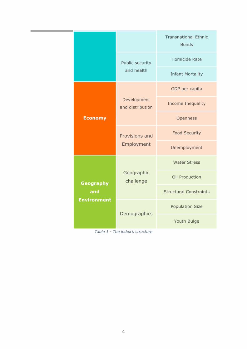
which are composed by 24 indicators. Table 2 and Table 3 (p.5 and p.8) gives details
about the variables (the raw data and where to download them). The data used are all
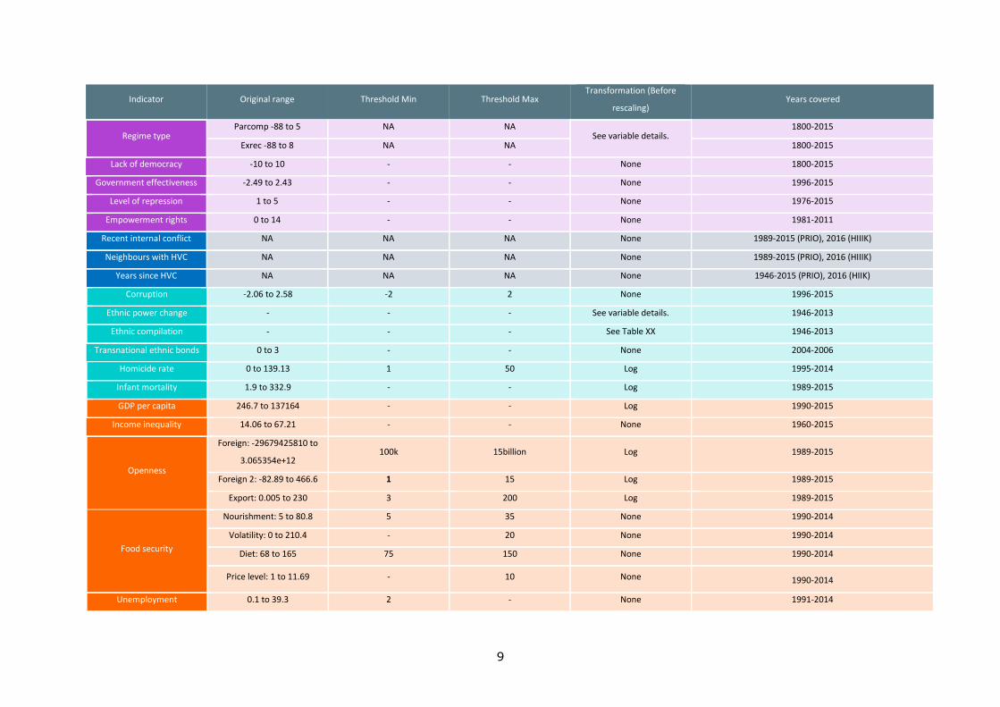
freely accessible by any user on the Internet. Table 4 (p.10) presents some descriptive
statistics: the original range of the data distribution, the thresholds imposed (min and
max), the transformation (logistic or of any other type) done before the rescaling and the
years covered by each original dataset.
Index Risk Area Concept Indicator
GC
RI I
nd
ex
Political
Regime type
Regime Type
Lack of Democracy
Regime
performance
Government
Effectiveness
Level of Repression
Empowerment Rights
Security
Current conflict
situation
Recent Internal Conflict
Neighbouring with HVC
History of
conflict Years since HVC
Social Social cohesion
and diversity
Corruption
Ethnic Power Change
Ethnic Compilation
4
Transnational Ethnic
Bonds
Public security
and health
Homicide Rate
Infant Mortality
Economy
Development
and distribution
GDP per capita
Income Inequality
Openness
Provisions and
Employment
Food Security
Unemployment
Geography
and
Environment
Geographic
challenge
Water Stress
Oil Production
Structural Constraints
Demographics
Population Size
Youth Bulge
Table 1 - The index’s structure

5
1 All datasets have been accessed on September 15th, 2017.
Table 2 - Variable sources (first part)1
Indicator Source Name of dataset Name of original indicator(s) URL
Regime type Center for Systemic Peace Polity IV Annual Time-Series,
1800-2015 PARCOM, EXREC http://www.systemicpeace.org/inscrdata.html
Lack of democracy Center for Systemic Peace Polity IV Annual Time-Series,
1800-2015 POLITY2 http://www.systemicpeace.org/inscrdata.html
Government effectiveness World Bank Government Effectiveness:
Estimate GE.EST
http://databank.worldbank.org/data/reports.aspx?source=worldwide-
governance-indicators
Level of repression Political Terror Scale Project PTS Data
Highest of the three indicators
in the set (PTS_A, PTS_H,
PTS_S)
http://www.politicalterrorscale.org/Data/Download.html
Empowerment rights CIRI Human Rights Data Project CIRI Data NEW_EMPINX http://www.humanrightsdata.com/p/data-documentation.html
Recent internal conflict HIIK; UCDP/PRIO
Battle related deaths, One-sided
violence, Non-state conflict,
Conflict Barometer 2016
Highest casualty estimates
http://ucdp.uu.se/downloads/
http://hiik.de/de/daten/ Neighbours with HVC HIIK; UCDP/PRIO
Battle related deaths, One-sided
violence, Non-state conflict,
Conflict Barometer 2016
Highest casualty estimates
Years since HVC HIIK; UCDP/PRIO Armed Conflict Dataset, Conflict
Barometer 2016 Conflicts of intensity level 2
Corruption World Bank Control of Corruption: Estimate CC.EST http://databank.worldbank.org/data/reports.aspx?source=worldwide-
governance-indicators
Ethnic Power Change ETH Zurich EPR Core Dataset Recording of dataset, see
variable page http://www.icr.ethz.ch/data/epr
6
Ethnic compilation ETH Zurich EPR Core Dataset Recording of dataset, see
variable page http://www.icr.ethz.ch/data/epr
Transnational ethnic bonds
CIDCM Center for International
Development &Conflict
Management
Marupdate_20042006 GC10 http://www.mar.umd.edu/mar_data.asp
Homicide rate World Bank World Development Indicators Intentional homicides (per
100,000 people) http://data.worldbank.org/indicator/VC.IHR.PSRC.P5
Infant mortality World Bank World Development Indicators Mortality rate, under-5 (per
1,000 live births) http://data.worldbank.org/indicator/SH.DYN.MORT

7
Indicator Source Name of dataset Name of original indicator(s) URL
GDP per capita World Bank World Development Indicators GDP per capita, PPP (constant 2011
international $) http://data.worldbank.org/indicator/NY.GDP.PCAP.PP.KD
Income inequality Harvard Dataverse Network
The Standardized World Income
Inequality Database
Net inequality https://dataverse.harvard.edu/dataset.xhtml?persistentId=hdl:1
902.1/11992
Openness Word Bank World Development Indicators
Foreign direct investment, net
inflows (BoP, current US$)
http://data.worldbank.org/indicator/BX.KLT.DINV.CD.WD
Foreign direct investment, net
inflows (% of GDP)
http://data.worldbank.org/indicator/BX.KLT.DINV.WD.GD.ZS
Exports of goods and services (% of
GDP)
http://data.worldbank.org/indicator/NE.EXP.GNFS.ZS
Food security FAO Food security indicators
Average dietary energy supply
adequacy
http://www.fao.org/economic/ess/ess-fs/ess-fadata/en/ Domestic food price index
Prevalence of undernourishment
Domestic food price volatility
Unemployment World Bank World Development Indicators
Unemployment, total (% of total
labour force) (modelled ILO
estimate)
http://data.worldbank.org/indicator/SL.UEM.TOTL.ZS
Water stress World Resources Institute Aqueduct Country and River Basin
Rankings (Raw country scores) tdefm
http://www.wri.org/resources/data-sets/aqueduct-country-and-
river-basin-rankings
Oil producer World Bank World Development Indicators Fuel exports (% of merchandise
exports) http://data.worldbank.org/indicator/TX.VAL.FUEL.ZS.UN
Structural constraints BTI: The Bertelsmann Stiftung BTI 2016 Structural constrains (Q13.1) http://www.bti-project.org/en/index/

8
2 All datasets have been accessed on September 15th, 2017.
Population size UN DESA/ Population Division Annual population by single age -
Both Sexes. Sum of all ages http://esa.un.org/unpd/wpp/Download/Standard/Interpolated/
Youth bulge UN DESA/ Population Division Annual population by single age -
Both Sexes.
Sum of ages 15-24 divided by sum
of ages 25+ http://esa.un.org/unpd/wpp/Download/Standard/Interpolated/
Table 3 - Variable sources (second part)2
9
Indicator Original range Threshold Min Threshold Max Transformation (Before
rescaling) Years covered
Regime type Parcomp -88 to 5 NA NA
See variable details. 1800-2015
Exrec -88 to 8 NA NA 1800-2015
Lack of democracy -10 to 10 - - None 1800-2015
Government effectiveness -2.49 to 2.43 - - None 1996-2015
Level of repression 1 to 5 - - None 1976-2015
Empowerment rights 0 to 14 - - None 1981-2011
Recent internal conflict NA NA NA None 1989-2015 (PRIO), 2016 (HIIIK)
Neighbours with HVC NA NA NA None 1989-2015 (PRIO), 2016 (HIIIK)
Years since HVC NA NA NA None 1946-2015 (PRIO), 2016 (HIIK)
Corruption -2.06 to 2.58 -2 2 None 1996-2015
Ethnic power change - - - See variable details. 1946-2013
Ethnic compilation - - - See Table XX 1946-2013
Transnational ethnic bonds 0 to 3 - - None 2004-2006
Homicide rate 0 to 139.13 1 50 Log 1995-2014
Infant mortality 1.9 to 332.9 - - Log 1989-2015
GDP per capita 246.7 to 137164 - - Log 1990-2015
Income inequality 14.06 to 67.21 - - None 1960-2015
Openness
Foreign: -29679425810 to
3.065354e+12 100k 15billion Log 1989-2015
Foreign 2: -82.89 to 466.6 1 15 Log 1989-2015
Export: 0.005 to 230 3 200 Log 1989-2015
Food security
Nourishment: 5 to 80.8 5 35 None 1990-2014
Volatility: 0 to 210.4 - 20 None 1990-2014
Diet: 68 to 165 75 150 None 1990-2014
Price level: 1 to 11.69 - 10 None 1990-2014
Unemployment 0.1 to 39.3 2 - None 1991-2014

10
Water stress 0.58 to 4.43 0.58 4.44 None NA
Oil producer 0 to 99.97 1 - Log 1989-2015
Structural constraints 1 to 10 - - None 2006-2016
Population size 0 to 1.38 billion 6 12.5 Log 1989-2016
Youth bulge 0.10 to 0.42 0.12 0.39 None 1989-2016
Table 4 - Descriptive statistics
11
3. Variable definition
The GCRI index is composed of 24 variables, grouped in 10 concepts, which are then
grouped in 5 risk areas. While Table 4 (p.10) provides some descriptive statistics, more
detailed information is available in the successive paragraphs. The purpose of the present
chapter is to describe in detail each variable and to explain the R code used for computing
the variables.
As presented in Table 4, data for calculating the Global Conflict Risk Index are extracted
from 14 different datasets. While some of the datasets are complete, others contain
missing data for specific years and/or specific countries. For each variable, the share of
available data is presented, as well as their geographical location. These graphical
representations (presented below within the variables’ descriptions) aim at providing an
understanding on the limitations of some variables and the limitations of some
geographical regions when it comes to producing and/or providing data.
In order to overcome the lack of data and be able to compute the model, the missing data
are imputed (replacing missing data with substituted values) and identified as exceptions.
In the imputation system adopted, data is taken from either the closest known historical
data (desk research is conducted for finding precise information which would then justify
the substituted value), or, if not possible, from regional averages, or from similar
countries. In this last case, the characteristics considered to identify a country as “similar”
are political, social-economic and/or geographic, according to what is acknowledged as
the most adequate one. Thereby, all missing data can be imputed in a relevant way
allowing the model to run trouble-free. The imputation is included in the data construction
phase, making the data a single and complete dataset ready for statistical analysis.
The 24 variables are used as input for the composite model.
3.1. Regime Type (REG_U)
Description: The regime type is one of the strongest indicators for the outbreak of
political violence. Empirical evidence shows that, with some restrictions, democracies
indeed do not resort to war against each other. The idea here is that some “side-effects”
of democracy, such as the rule of law, a certain level of socio-economic development, and
the inclusion into international trade networks, contribute to a more peaceful way of
solving conflicts. The regime type indicator is designed to capture the effect of the
democratic U-curve, where anocracies are seen as inherently less stable than autocracies
and democracies (Hegre, 2001).
12
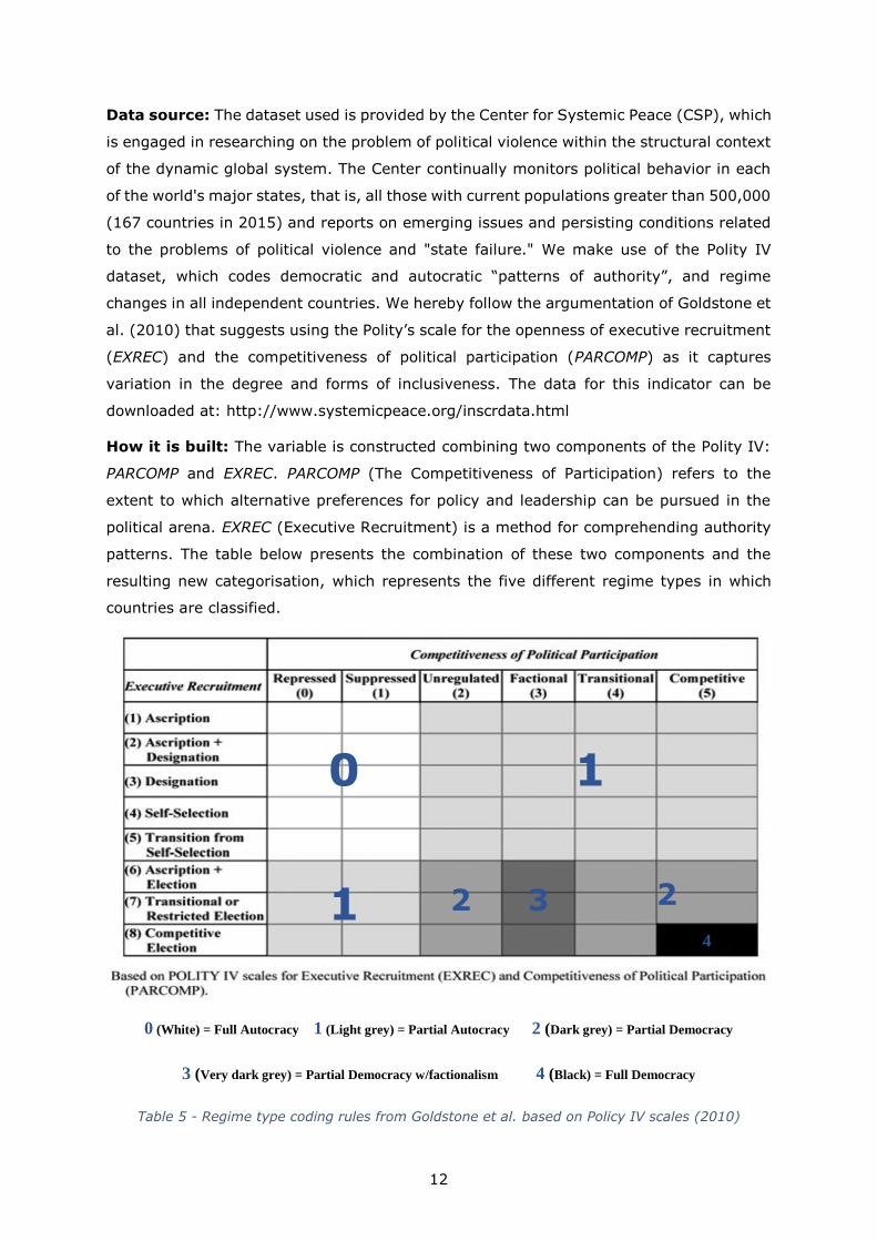
Data source: The dataset used is provided by the Center for Systemic Peace (CSP), which
is engaged in researching on the problem of political violence within the structural context
of the dynamic global system. The Center continually monitors political behavior in each
of the world's major states, that is, all those with current populations greater than 500,000
(167 countries in 2015) and reports on emerging issues and persisting conditions related
to the problems of political violence and "state failure." We make use of the Polity IV
dataset, which codes democratic and autocratic “patterns of authority”, and regime
changes in all independent countries. We hereby follow the argumentation of Goldstone et
al. (2010) that suggests using the Polity’s scale for the openness of executive recruitment
(EXREC) and the competitiveness of political participation (PARCOMP) as it captures
variation in the degree and forms of inclusiveness. The data for this indicator can be
downloaded at: http://www.systemicpeace.org/inscrdata.html
How it is built: The variable is constructed combining two components of the Polity IV:
PARCOMP and EXREC. PARCOMP (The Competitiveness of Participation) refers to the
extent to which alternative preferences for policy and leadership can be pursued in the
political arena. EXREC (Executive Recruitment) is a method for comprehending authority
patterns. The table below presents the combination of these two components and the
resulting new categorisation, which represents the five different regime types in which
countries are classified.
0 (White) = Full Autocracy 1 (Light grey) = Partial Autocracy 2 (Dark grey) = Partial Democracy
3 (Very dark grey) = Partial Democracy w/factionalism 4 (Black) = Full Democracy
Table 5 - Regime type coding rules from Goldstone et al. based on Policy IV scales (2010)
1 0
1 2 2 3
4

13
The countries that did not match any of the above mentioned regime types are classified
under “foreign intervention” (6 and 7) and “transition” (8).
Based on this categorization, a new score is associated to each regime type as presented
in the Table 6.
Type:
Full d
em
ocra
cy
Full a
uto
cra
cy
Part
ial dem
ocra
cy
Part
ial auto
cra
cy
Tra
nsitio
n
Part
ial
dem
ocra
cy
w/f
actionalism
Fore
ign I
nte
rvention
Regime
type
coding
rules
(Table
5)
4 0 2 1 8 3 6 and 7
Score: 1 1.07 3.91 3.98 4.49 10 10
Table 6 - Regime type scores
Descriptive Statistics: Missing data are imputed taking the closest available value.
The average percentage of available raw data is 95.4%. The remaining 4.6% is imputed.
The distribution of raw data by year shows that, in this variable, we always have a high
availability of data.

14
Table 7 - Data availability per year for the variable “Regime Type”
Citations: According to Vreeland, anocracies are more susceptible to civil war than either
pure democracies or pure dictatorships’ (Vreeland, 2008, p. 401). Other studies confirm
this claim (Ellingsen, 2000; Collier & Hoeffler, Greed and Grievance in civil wars, 2004;
Hegre, Ellingsen, Gates, & Gleditsch, 2001; Russett, Oneal, & Cox, 2000).
Practically, all quantitative studies rely on the Polity dataset, which provides global
coverage and open source access and is frequently updated (Collier & Hoeffler 2004; Hegre
2002; Goldstone et al. 2010).
0%
10%
20%
30%
40%
50%
60%
70%
80%
90%
100%
19
89
19
90
19
91
19
92
19
93
19
94
19
95
19
96
19
97
19
98
19
99
20
00
20
01
20
02
20
03
20
04
20
05
20
06
20
07
20
08
20
09
20
10
20
11
20
12
20
13
20
14
20
15
20
16
Figure 1 - Data availability per country for the variable “Regime Type”
15
Collier, P. & Hoeffler, A. 2004. Greed and Grievance in civil wars. Oxford Economic Papers
56, pp. 563-596.
Goldstone, J. A. et al. 2010. A Global Model for Forecasting Political Instability. American
Journal of Political Science 54, pp. 190-208.
Hegre, H. & Sambanis, N. 2006. Sensitivity Analysis of Empirical Results on Civil War
Onset. 4th ed. Journal of Conflict Resolution 50, pp. 508-536.
Vreeland, J. 2008. The Effect of Political Regime on Civil War: Unpacking Anocracy. 3rd ed.
Journal of Conflict Resolution 52, pp. 401-425.
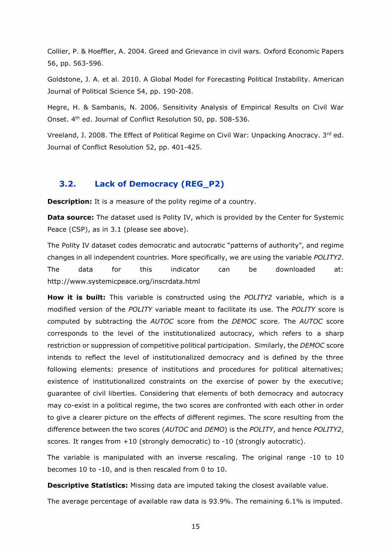
3.2. Lack of Democracy (REG_P2)
Description: It is a measure of the polity regime of a country.
Data source: The dataset used is Polity IV, which is provided by the Center for Systemic
Peace (CSP), as in 3.1 (please see above).
The Polity IV dataset codes democratic and autocratic “patterns of authority”, and regime
changes in all independent countries. More specifically, we are using the variable POLITY2.
The data for this indicator can be downloaded at:
http://www.systemicpeace.org/inscrdata.html
How it is built: This variable is constructed using the POLITY2 variable, which is a
modified version of the POLITY variable meant to facilitate its use. The POLITY score is
computed by subtracting the AUTOC score from the DEMOC score. The AUTOC score
corresponds to the level of the institutionalized autocracy, which refers to a sharp
restriction or suppression of competitive political participation. Similarly, the DEMOC score
intends to reflect the level of institutionalized democracy and is defined by the three
following elements: presence of institutions and procedures for political alternatives;
existence of institutionalized constraints on the exercise of power by the executive;
guarantee of civil liberties. Considering that elements of both democracy and autocracy
may co-exist in a political regime, the two scores are confronted with each other in order
to give a clearer picture on the effects of different regimes. The score resulting from the
difference between the two scores (AUTOC and DEMO) is the POLITY, and hence POLITY2,
scores. It ranges from +10 (strongly democratic) to -10 (strongly autocratic).
The variable is manipulated with an inverse rescaling. The original range -10 to 10
becomes 10 to -10, and is then rescaled from 0 to 10.
Descriptive Statistics: Missing data are imputed taking the closest available value.
The average percentage of available raw data is 93.9%. The remaining 6.1% is imputed.

16
The distribution of raw data by year shows that there is always a high coverage of data
across time.
Table 8 - Data availability per year for the variable “Lack of Democracy"
Figure 2 - Data availability per country for the variable “Lack of Democracy"
Citations: Robert Dahl defines democracy as effective participation, voting equality,
knowledge on the issue and its alternatives, control over what issues are placed on the
agenda, and all or most adults should be included in the process (Dahl, Robert A. 1998.
On Democracy. New Haven: Yale UP, pp. 36-38).
0%
10%
20%
30%
40%
50%
60%
70%
80%
90%
100%1
98
9
19
90
19
91
19
92
19
93
19
94
19
95
19
96
19
97
19
98
19
99
20
00
20
01
20
02
20
03
20
04
20
05
20
06
20
07
20
08
20
09
20
10
20
11
20
12
20
13
20
14
20
15
20
16

17
3.3. Government effectiveness (GOV_EFF)
Description: Government Effectiveness measures the quality of social and political
indicators, as it is perceived by citizens. Public and civil service, policy formulation,
credibility of the government are the main topics monitored.
Data source: The dataset used is the World Bank’s Worldwide Governance Indicators,
which are “aggregate and individual governance indicators for 215 countries and territories
over the period 1996–2015, for six dimensions of governance.”3 (The data are available
for download at: http://data.worldbank.org/data-catalog/worldwide-governance-
indicators). In this case we are using the series “Government Effectiveness: Estimate”.
How it is built: The variable used presents country's score on the aggregate indicator, in
units of a standard normal distribution. The original variable ranges approximately from -
2.5 to 2.5.
The variable values are then manipulated with an inverse rescaling in order to be
transformed to a 0 to 10 scale.
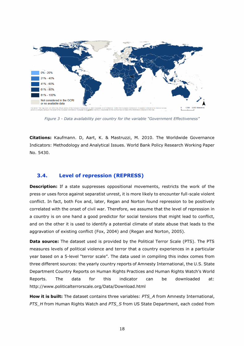
Descriptive Statistics: Missing data are imputed taking the closest available value.
The average percentage of available raw data is 62.5%. The remaining 37.5% is imputed.
The distribution of raw data by year shows that we have complete data only as of 2002.
Table 9 - Data availability per year for the variable “Government Effectiveness”
3 World Bank Website.
0%
10%
20%
30%
40%
50%
60%
70%
80%
90%
100%
19
89
19
90
19
91
19
92
19
93
19
94
19
95
19
96
19
97
19
98
19
99
20
00
20
01
20
02
20
03
20
04
20
05
20
06
20
07
20
08
20
09
20
10
20
11
20
12
20
13
20
14
20
15
20
16
18
Figure 3 - Data availability per country for the variable “Government Effectiveness”
Citations: Kaufmann. D, Aart, K. & Mastruzzi, M. 2010. The Worldwide Governance
Indicators: Methodology and Analytical Issues. World Bank Policy Research Working Paper
No. 5430.
3.4. Level of repression (REPRESS)
Description: If a state suppresses oppositional movements, restricts the work of the
press or uses force against separatist unrest, it is more likely to encounter full-scale violent
conflict. In fact, both Fox and, later, Regan and Norton found repression to be positively
correlated with the onset of civil war. Therefore, we assume that the level of repression in
a country is on one hand a good predictor for social tensions that might lead to conflict,
and on the other it is used to identify a potential climate of state abuse that leads to the
aggravation of existing conflict (Fox, 2004) and (Regan and Norton, 2005).
Data source: The dataset used is provided by the Political Terror Scale (PTS). The PTS
measures levels of political violence and terror that a country experiences in a particular
year based on a 5-level “terror scale”. The data used in compiling this index comes from
three different sources: the yearly country reports of Amnesty International, the U.S. State
Department Country Reports on Human Rights Practices and Human Rights Watch’s World
Reports. The data for this indicator can be downloaded at:
http://www.politicalterrorscale.org/Data/Download.html
How it is built: The dataset contains three variables: PTS_A from Amnesty International,
PTS_H from Human Rights Watch and PTS_S from US State Department, each coded from
19
1 to 5. The highest score of the three variables is used as the repression variable and
rescaled from 0 to 10.
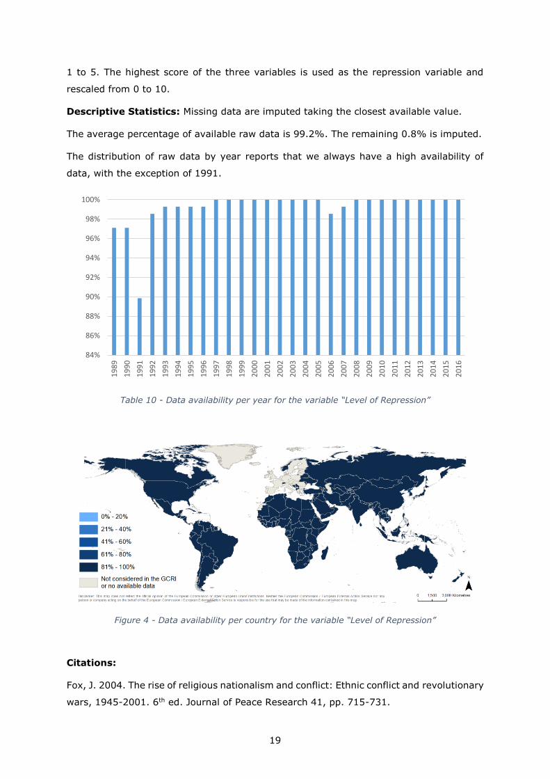
Descriptive Statistics: Missing data are imputed taking the closest available value.
The average percentage of available raw data is 99.2%. The remaining 0.8% is imputed.
The distribution of raw data by year reports that we always have a high availability of
data, with the exception of 1991.
Table 10 - Data availability per year for the variable “Level of Repression”
Figure 4 - Data availability per country for the variable “Level of Repression”
Citations:
Fox, J. 2004. The rise of religious nationalism and conflict: Ethnic conflict and revolutionary
wars, 1945-2001. 6th ed. Journal of Peace Research 41, pp. 715-731.
84%
86%
88%
90%
92%
94%
96%
98%
100%
19
89
19
90
19
91
19
92
19
93
19
94
19
95
19
96
19
97
19
98
19
99
20
00
20
01
20
02
20
03
20
04
20
05
20
06
20
07
20
08
20
09
20
10
20
11
20
12
20
13
20
14
20
15
20
16
20
Regan, P. M. & Norton, D. 2005. Greed, Grievance and Mobilization in Civil Wars. 3rd ed.
Journal of Conflict Resolution 49, pp. 319-336.
3.5. Empowerment rights (EMPOWER)
Description: Every political system claims to provide a certain set of civil rights, as the
very legitimacy of a government lies in providing services and granting rights for its
citizens. According to Merkel et al. (2003), the rule of law together with a system of checks
and balances, as well as the granting of civil rights constitute three of the five pillars of a
functioning political system. If one or several of these subsystems show deficiencies,
conflicts are much likelier to erupt (Merkel et al., 2003).
Data source: The Empowerment Rights index, provided by the CIRI Human Rights data
project, is being used here. The CIRI Human Rights Dataset contains standards-based
quantitative information on government. More specifically, the information gathered deals
with a wide range of human rights, internationally recognized, for countries of all regime
types and from all regions of the world. The data for this indicator can be downloaded at:
http://www.humanrightsdata.com/p/data-documentation.html.
How it is built: The Empowerment Rights Index, called NEW_EMPINX variable in the
dataset, is based on seven indicators: the Foreign Movement, Domestic Movement,
Freedom of Speech, Freedom of Assembly & Association, Workers’ Rights, Electoral Self-
Determination, and Freedom of Religion. It ranges from 0 (no government respect for
these seven rights) to 14 (full government respect for these seven rights). The original
range 0 to 14 becomes 14 to 0, and is then rescaled from 0 to 10.
Descriptive Statistics: Missing data are imputed taking the closest available value.
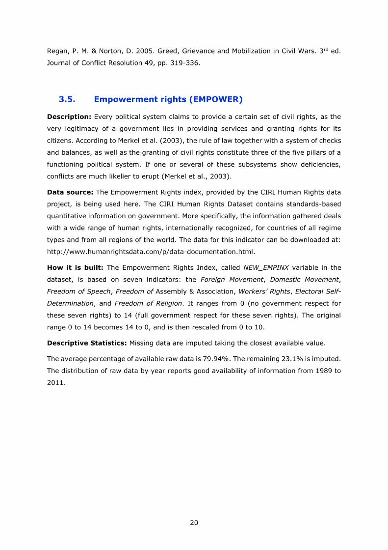
The average percentage of available raw data is 79.94%. The remaining 23.1% is imputed.
The distribution of raw data by year reports good availability of information from 1989 to
2011.

21
Table 11 - Data availability per year for the variable “Empowerment Rights”
Figure 5 - Data availability per country for the variable “Empowerment Rights”
Citations: Poe, Steven P. Carey, Sabine C. & Vazquez, Tanya C. 2001. How are these
pictures Different? A quantitative comparison of the US State Department and Amnesty
International human rights reports, 1976-1995. Human Rights Quarterly 23.3, pp. 650-
677.
Merkel, W. e. a. 2003. Defekte Demokratie Bd. 1: Theorie. Wiesbaden: VS Verlag für
Sozialwissenschaften.
0%
10%
20%
30%
40%
50%
60%
70%
80%
90%
100%
19
89
19
90
19
91
19
92
19
93
19
94
19
95
19
96
19
97
19
98
19
99
20
00
20
01
20
02
20
03
20
04
20
05
20
06
20
07
20
08
20
09
20
10
20
11
20
12
20
13
20
14
20
15
20
16

22
3.6. Recent Internal Conflict (CON_INT)
Description: This variable takes into account all the conflicts that have happened since
1989 and classifies the conflicts based on their types (national or subnational). Moreover,
it measures the intensity of the conflict (based on the number of battle-related deaths).
Data source: The three datasets used in the computation of this variable, are provided
by UCDP/PRIO Armed Conflict Dataset. This is a joint research project between the Uppsala
Conflict Data Program (UCDP) at the Department of Peace and Conflict Research Uppsala
University and the Centre for the Study of Civil War at the International Peace Research
Institute in Oslo (PRIO). The datasets used are: UCDP Battle-Related Deaths Dataset
(BRD), UCDP One-sided Violence (OSV) and UCDP Non-State Conflict datasets (NSC). The
first dataset contains information on the number of battle-related deaths in conflicts from
1989 to 2016. The second dataset provides data on intentional attacks on civilians by
governments and formally organized armed groups. The third one collects information on
armed conflict where none of the parties is the government of a state. The data for this
indicator can be downloaded at: http://ucdp.uu.se/downloads/.
How it is built: To create the variable Recent Internal Conflict, three databases are used.
For each of these three databases, statistical methods are applied. For all three databases
we reclassify the data into two categories: National and Subnational. The outputs are three
new datasets, which are then bound together in order to obtain the final scores.
Concerning the first dataset called BRD (Battle-Related Deaths Dataset), two variables are
used: Incomp (a general coding of the conflict issue) and Typeofconflict. This last one
classifies conflicts in four different categories: extra-systemic (1), interstate (2), internal
(3) and internationalized internal (4). The Typeofconflict extra-systemic (1) and interstate
(2) are not used by the GCRI. Based on the two variables, we reclassify the conflicts into
two categories (national and subnational) as shown in the table below.
Type of conflict
Incompatibility
3 4
1 Subnational Subnational
2 National National
A score of intensity is given to both national and subnational conflicts. Based on the
existing column BdHigh of the BRD dataset, a new column called Intensity is created. It

23
ranges from 0 to 3 according to the following rules: BdHigh values<25 deaths = 0; 25-
499 deaths = 1; 500-999 deaths = 2, >1000 deaths = 3.
The second dataset used is the OSV (One-sided Violence). We make a subset keeping only
the cases when the actors involved are governments. Then we create a new column called
SN (Subnational) and we apply a value range from 0 to 3 based on the existing
HighFatalityEstimate column of the OSV dataset, according to the following rules:
HighFatalityEstimate > 500 = 2, HighFatalityEstimate > 1000 = 3.
The third dataset used is NSC (Non-State Conflict datasets). In case conflicts happened in
more than one country, then they are attributed to just one country. Following this we
create a new column called SN (Subnational) and we apply a value range from 0 to 3
based on the existing HighFatalityEstimate column of the NSC dataset, according to the
following rules: HighFatalityEstimate > 500 = 2, HighFatalityEstimate > 1000 = 3.
We extract a subset from BRD considering only the subnational conflicts, then we append
to it OSV and NSC in order to obtain a list of all the subnational conflicts. This list contains
more than one record for each country/year. We apply two different functions to the list.
The first function is the max of the SN score, and it is used to calculate the highest SN
value for each country/year record. The second function is the sum of the column count.
We create this column in order to count the conflicts, therefore each record has a default
value of 1. The intensity indicator for subnational conflicts is created combining the SN
and Count column, as shown in the Table 12 below. In this way we obtain the intensity
table.
Count
Intensity
1 2 >2
1 5 6 7
2 8 8.5 9
3 10 10 10
Table 12 - Subnational Intensity
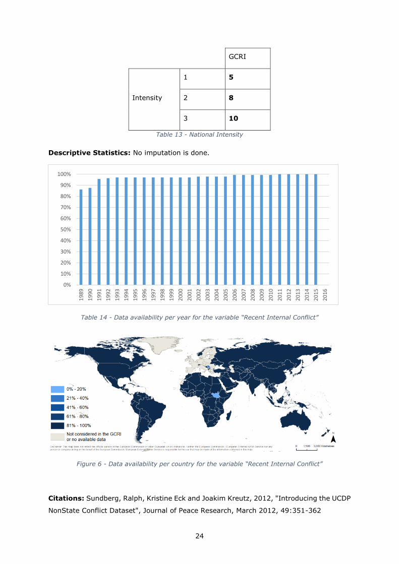
We create a second subset from BRD, this time considering only the national conflicts. The
intensity indicator for national conflicts is created as shown in the Table 13 below.
24
GCRI
Intensity
1 5
2 8
3 10
Table 13 - National Intensity
Descriptive Statistics: No imputation is done.
Table 14 - Data availability per year for the variable “Recent Internal Conflict”
Figure 6 - Data availability per country for the variable “Recent Internal Conflict”
Citations: Sundberg, Ralph, Kristine Eck and Joakim Kreutz, 2012, "Introducing the UCDP
NonState Conflict Dataset", Journal of Peace Research, March 2012, 49:351-362
0%
10%
20%
30%
40%
50%
60%
70%
80%
90%
100%
19
89
19
90
19
91
19
92
19
93
19
94
19
95
19
96
19
97
19
98
19
99
20
00
20
01
20
02
20
03
20
04
20
05
20
06
20
07
20
08
20
09
20
10
20
11
20
12
20
13
20
14
20
15
20
16

25
Eck, Kristine and Lisa Hultman, 2007. ‘One-sided violence against civilians in war: insights
from new fatality data´, Journal of Peace Research 44(2): 233-246.
Allansson, Marie, Erik Melander & Lotta Themnér (2017) Organized violence, 1989-2016.
Journal of Peace Research 54(4).
Complementary dataset
The UCDP/PRIO Armed Conflict Dataset is updated until 2015, and for this reason we use
a different dataset to cover the 2016. The dataset for 2016 is provided by the Heidelberg
Institute for International Conflict Research (HIIK), which is an independent research
association affiliated with the Department of Political Science at the University of
Heidelberg. The dataset, named Conflict Barometer 2016, is an analysis of global conflicts,
whether they are wars, crises, or peace negotiations.
We use two different files: the HIIK dataset and the Inform list, which is a name list with
country codes.
We use a max function to identify the max intensity of all the conflicts for each country,
then we count how many conflicts with that intensity are associable to each state.
A rescaling is applied according to the following table.
HIIK Based
PRIO/UCDP
Based
GCRI
Intensity
HIIK
intensity
Number of conflicts (of highest HIIK
intensity)
Casualties Number of
conflicts
0 0
<25
1 1
-
2 2 1 -
3 2 2 -
4 2 >2 -
5 3 1 25-499 1
6 3 2 25-499 2
7 3 >2 25-499 >2
8 4 1 500-999 1
8.5 4 2 500-999 2
9 4 >2 500-999 >2
26
10 5
>=1000
3.7. Neighbouring Conflict (CON_NB)
Description: Another factor that strongly correlates with violent conflict is the conflict
situation in neighbouring countries. Sambanis stated in 2001: “Living in a bad
neighbourhood can triple a country’s chance of having an ethnic war” (2001). Hegre and
Sambanis (2006) find that the positive impact of neighbouring conflict on the risk of civil
war remains robust under many possible specifications, and war in adjacent countries has
also been suggested as useful for predicting conflict or generating ‘early warning’ systems
(Hegre & Sambanis, 2006; Esty, Goldstone, Gurr, Harff, & Unger, 1998; Gleditsch, 2007).
In addition, there is evidence that conflicts raise the level of repression in neighbouring
countries, this in turn leading to national power conflicts (Danneman & Ritter, 2014).
This "spill-over effect" between countries is modelled by the inclusion of a neighbourhood
variable. This variable represents the highest conflict intensity that neighbouring countries
(of country A) have in both dimensions, national and subnational.
Data source: To construct this variable we combine the output produced with the Recent
internal conflict variable, with a matrix produced with the R package “cshapes” designed
by Nils B.Weidmann. This data package defines which country borders with which other
country.
How it is built: Once the matrix GCRI_NB is created (it is the matrix that associates each
country with all his neighbours for all the years), we create a subset in order to consider
only the conflicts between countries and to exclude the internal ones. We merge the
previous file with the recent internal conflict output. At this point we have three columns:
country A, country B, and the conflict intensity of B. We use the max function so that for
each year country A is associated with just one country B, the one that has the highest
conflict intensity score.
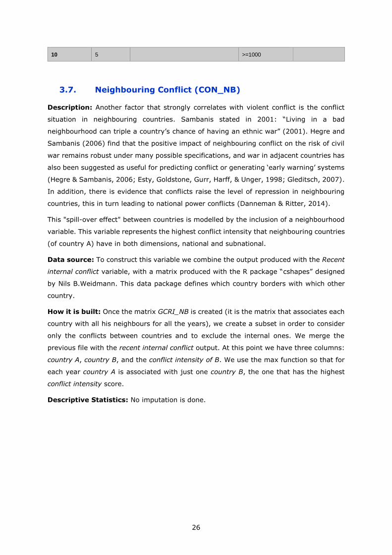
Descriptive Statistics: No imputation is done.
27
Table 15 - Data availability per year for the variable “Neighbouring Conflict”
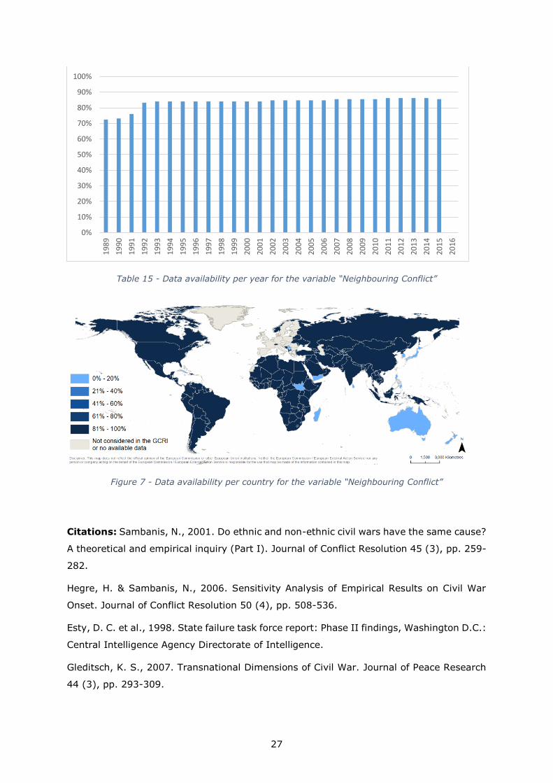
Figure 7 - Data availability per country for the variable “Neighbouring Conflict”
Citations: Sambanis, N., 2001. Do ethnic and non-ethnic civil wars have the same cause?
A theoretical and empirical inquiry (Part I). Journal of Conflict Resolution 45 (3), pp. 259-
282.
Hegre, H. & Sambanis, N., 2006. Sensitivity Analysis of Empirical Results on Civil War
Onset. Journal of Conflict Resolution 50 (4), pp. 508-536.
Esty, D. C. et al., 1998. State failure task force report: Phase II findings, Washington D.C.:
Central Intelligence Agency Directorate of Intelligence.
Gleditsch, K. S., 2007. Transnational Dimensions of Civil War. Journal of Peace Research
44 (3), pp. 293-309.
0%
10%
20%
30%
40%
50%
60%
70%
80%
90%
100%
19
89
19
90
19
91
19
92
19
93
19
94
19
95
19
96
19
97
19
98
19
99
20
00
20
01
20
02
20
03
20
04
20
05
20
06
20
07
20
08
20
09
20
10
20
11
20
12
20
13
20
14
20
15
20
16
28
Danneman, N. & Hencken Ritter, E., 2014. Contagious Rebellion and Preemptive
Repression. Journal of Conflict Resolution 58 (2), pp. 254-279.
Complementary dataset
As in 3.6, in order to have data also for 2016, it is necessary to use data beyond the
UCDP/PRIO Armed Conflict Dataset, which is updated until 2015. Therefore, the dataset
for 2016 is provided by the Heidelberg Institute for International Conflict Research (HIIK).
The dataset used to calculate the Neighbouring Conflict values (CON_NB) is the 2016 HIIK
Conflict Intensity (HIIK CON_INT). We first associate all the countries in HIIK CON_INT
with their neighbours using a matrix of distances. Then we calculate CON_NB as the
maximum HIIK CON_INT of the neighbours.
3.8. Years Since Highly Violent Conflict (YRS_HVC)
Description: Countries previously engaged in civil war have a high probability of
experiencing renewed violence or perpetuating conflict, even outbreak of numerous violent
conflicts at the same time. This phenomenon is the so-called “War Trap” (Bueno de
Mesquita, 1983) or “Conflict Trap” (Collier, et al., 2003), which is identified as a significant
predictor in many quantitative studies. Dixon (2009) lists eleven studies that found the
years since the last highly violent conflict to be highly significant in predicting the outbreak
of renewed violence.
This variable measures how many years have passed since a major conflict event has
taken place. It is an inverted count of years starting from the last high violent conflict in
the country and going back till a maximum of 10 years.
Data source: The dataset is provided by UCDP/PRIO Armed Conflict Dataset, as above
(see 3.6). The dataset used is Armed Conflict Dataset version 17.1, which collects
information on armed conflict where at least one party is the government of a state in the
time period 1946-2016. The data for this indicator can be downloaded at:
http://ucdp.uu.se/downloads/.
How it is built: We make a subset of the original dataset in order to exclude all those
cases where the intensity level is below 2. We reclassify the conflicts into two new columns
as presented in the following table:

29
Type of conflict
Incompatibility
3 4
1 Subnational (1) Subnational (1)
2 National (1) National (1)
We keep only the cases that fit in the above table.
We create the new column unicode. In this way a unique code, created by associating the
year with the location, is assigned to each record. We verify if there are double records,
and subsequently we eliminate them. A column called HVC is created equal to 1.
We apply the function that calculates the years since the last high violent conflict. We
make all the records >10 equal to 10, then an inverse rescaling from 10 to 0 is performed.
Descriptive Statistics: No imputation is done.
Table 16 - Data availability per year for the variable “Years Since Highly Violent Conflict “
0%
10%
20%
30%
40%
50%
60%
70%
80%
90%
100%
19
89
19
90
19
91
19
92
19
93
19
94
19
95
19
96
19
97
19
98
19
99
20
00
20
01
20
02
20
03
20
04
20
05
20
06
20
07
20
08
20
09
20
10
20
11
20
12
20
13
20
14
20
15
20
16

30
Figure 8 - Data availability per country for the variable “Years Since Highly Violent Conflict”
Citations: Bueno de Mesquita, B., 1983. The War Trap. Yale: Yale University Press.
Collier, P. et al., 2003. Breaking the Conflict Trap. Civil War and Development Policy. A
World Bank Policy Research Report. Oxford: Oxford University Press.
Dixon, J., 2009. What causes civil wars? Integrating Quantitative Research Findings.
International Studies Review 11, pp. 707-735.
Complementary dataset
As for the previous two variables, it is necessary to use a different dataset to cover the
reference year "2016". Data for this year are provided by the Heidelberg Institute for
International Conflict Research (HIIK), as in 3.6 and 3.7 (see above).
For this variable we use two different files: the processed 2015 HIIK dataset and the 2016
HIIK Conflict Intensity output. We apply the following rule to obtain values for Years since
HVC: if the variable CON_INT (from dataset 2016 Conflict Intensity) is >= 8 then Years
since HVC is 10. If CON_INT is < 8, then we use the value of column YRS_HVC from HIIK
2015 dataset minus 1.
3.9. Corruption (CORRUPT)
Description: Former World Bank President James Wolfensohn has many times called
corruption “the single greatest obstacle” to long-term development. In general, corruption
has proven to be one of the main challenges that post-conflict and in-transition countries
have to face and address as soon as possible. In fact, there had been many cases when
concerns about corruption have proven fatal to countries in delicate situations. If
31
corruption becomes endemic, then it can jeopardise both the political process and the
economic development of the state (O’Donnell, 2014).
Corruption measures the citizens' perception of how much public power is used for private
gain, and how important is the influence of private interests on the state.
Data source The dataset used is the World Bank’s Worldwide Governance Indicators, as
in 3.3 (please see above) (The data are available for download at:
http://data.worldbank.org/data-catalog/worldwide-governance-indicators). In this case
we are using the series “Control of Corruption”.
How it is built: The variable used presents country's score on the aggregate indicator, in
units of a standard normal distribution. The original variable ranges from -2,5 to 2,5.
Due to outliers, a minimum value of -2 and a maximum value of 2 are enforced. The
variable is imputed and rescaled from 0 to 10.
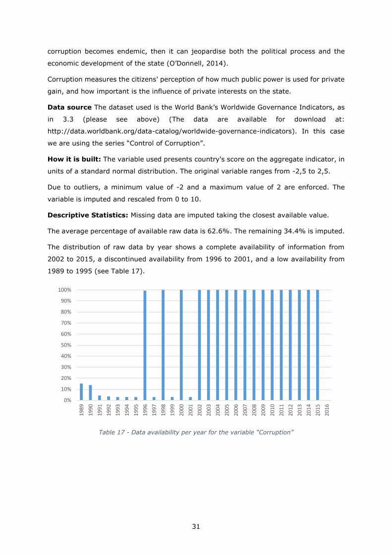
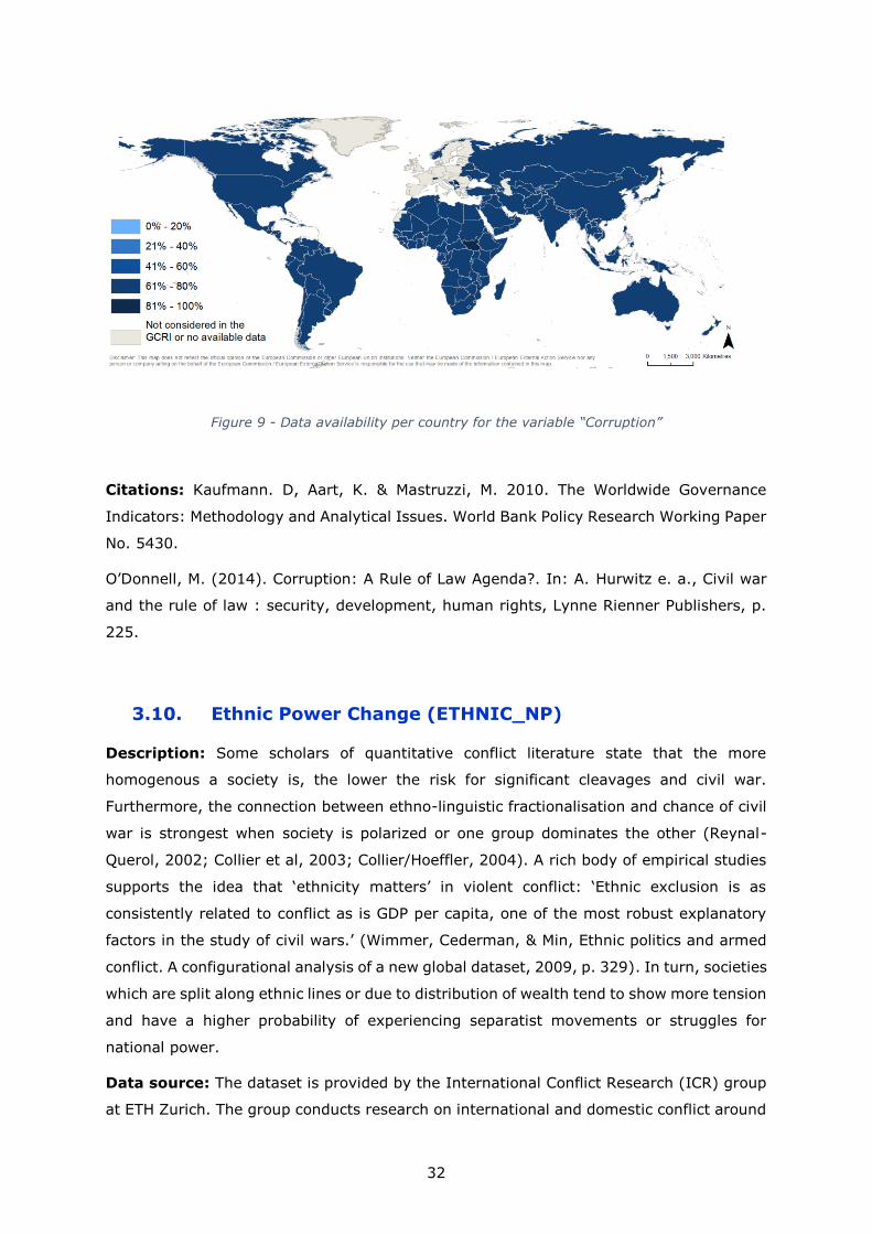
Descriptive Statistics: Missing data are imputed taking the closest available value.
The average percentage of available raw data is 62.6%. The remaining 34.4% is imputed.
The distribution of raw data by year shows a complete availability of information from
2002 to 2015, a discontinued availability from 1996 to 2001, and a low availability from
1989 to 1995 (see Table 17).
Table 17 - Data availability per year for the variable “Corruption”
0%
10%
20%
30%
40%
50%
60%
70%
80%
90%
100%
19
89
19
90
19
91
19
92
19
93
19
94
19
95
19
96
19
97
19
98
19
99
20
00
20
01
20
02
20
03
20
04
20
05
20
06
20
07
20
08
20
09
20
10
20
11
20
12
20
13
20
14
20
15
20
16
32
Figure 9 - Data availability per country for the variable “Corruption”
Citations: Kaufmann. D, Aart, K. & Mastruzzi, M. 2010. The Worldwide Governance
Indicators: Methodology and Analytical Issues. World Bank Policy Research Working Paper
No. 5430.
O’Donnell, M. (2014). Corruption: A Rule of Law Agenda?. In: A. Hurwitz e. a., Civil war
and the rule of law : security, development, human rights, Lynne Rienner Publishers, p.
225.
3.10. Ethnic Power Change (ETHNIC_NP)
Description: Some scholars of quantitative conflict literature state that the more
homogenous a society is, the lower the risk for significant cleavages and civil war.
Furthermore, the connection between ethno-linguistic fractionalisation and chance of civil
war is strongest when society is polarized or one group dominates the other (Reynal-
Querol, 2002; Collier et al, 2003; Collier/Hoeffler, 2004). A rich body of empirical studies
supports the idea that ‘ethnicity matters’ in violent conflict: ‘Ethnic exclusion is as
consistently related to conflict as is GDP per capita, one of the most robust explanatory
factors in the study of civil wars.’ (Wimmer, Cederman, & Min, Ethnic politics and armed
conflict. A configurational analysis of a new global dataset, 2009, p. 329). In turn, societies
which are split along ethnic lines or due to distribution of wealth tend to show more tension
and have a higher probability of experiencing separatist movements or struggles for
national power.
Data source: The dataset is provided by the International Conflict Research (ICR) group
at ETH Zurich. The group conducts research on international and domestic conflict around
33
the world. In recent years the group has been investigating the role of ethnic groups in
conflict, especially civil war, and their present research focuses on the link between ethnic
inequality and conflict. The dataset used is the EPR Core dataset, which records the access
to state power by all the ethnic groups of some political significance. It codes to which
level the group representative have held state power (from total control of the government
to overt political discrimination). The dataset provides data from 1946 till 2013 for all the
countries of the world. The data for this indicator can be downloaded at:
http://www.icr.ethz.ch/data/epr.
How it is built: The final variable transition measures the risk of conflict due to a change
in the distribution of state power among ethnic groups. It is scaled from 0 (no or irrelevant
power change with no strong ethnical domination) to 10 (power change with domination
of one group). The score for the variable transition is obtained by comparing seven
different variables on power change and power access. Among the seven variables used
(listed below), two are given by the EPR Core dataset and five are built by JRC.
Status (EPR Core dataset): it represents the amount of power owned by an ethnic group.
Power access is classified in nine categories (Dominant, Monopoly, Senior partner, Junior
partner, Powerless, Self-exclusion, Discriminated, Irrelevant, State collapsed), depending
on whether a group controls power alone, shares it with other ethnic groups, or is excluded
from it.
Status_lag (created by JRC): Using the variable Status, a lag4 is calculated in order to
analyse the change of status in the last year.
Reg_aut (EPR Core dataset): In addition to the previous variables which refer to the
national dimension of power, the EPR Core Dataset measures also the access to executive
power at the regional level. The variable in question is a separate regional autonomy
variable.
Reg_aut_lag (created by JRC): Using the variable Reg_aut, a lag is calculated in order to
analyse the change of access to executive power at the regional level in the last year.
Reg_aut_trans (created by JRC): It calculates the difference between the variables
Reg_aut and Reg_aut_lag in order to analyse the possible transition in the regional
autonomy.
4 A lag refers to a difference in time between an observation and a previous observation. (Eurostat
Statistics Explained, Glossary. Available at: http://ec.europa.eu/eurostat/statistics-
explained/index.php/Glossary:Lag. Retrieved on 26/07/2017)

34
Incexc (created by JRC): Using the variable Status, the results are categorised into four
new categories (Excluded, Included, Irrelevant, State collapse). The table below describes
the new categorisation:
INCEXC CLASSES
Excluded
(EXC)
Included
(INC)
Irrelevant
(IRR)
State
collapsed
(COL)
STATU
S
Dominant - x - -
Monopoly - x - -
Senior partner - x - -
Junior partner - x - -
Powerless x - - -
Self-exclusion x - - -
Discriminated x - - -
Irrelevant - - x -
State collapsed - - - x
Incexc_lag (created by JRC): Using the variable Incexc, a lag is calculated in order to
analyse the shift, if any, between exclusion and inclusion in the past years.
Specific comparisons are then conducted on the seven former variables. The outcomes of
these comparisons are the final scores. Below all the tables used for the comparisons (each
including always two variables) and the associated scores are presented.

35
INCEXC_LAG IN
CEXC
INC EXC
INC 0 -
EXC - 0
STATUS_LAG
Domin
ant
Monop
oly
Seni
or
part
ner
Juni
or
part
ner
Powerl
ess
Self-
exclus
ion
discrimin
ated
irrelev
ant
State
collap
sed
STATU
S
Dominan
t 0 - - -
- - - - -
Monopoly - 0 - - - - - - -
Senior
partner - - 0 -
- - - - -
Junior
partner - - - 0
- - - - -
Powerles
s - - - -
0 0 - - -
Self-
exclusion - - - -
6 0 6 6 -
Discrimin
ated - - - -
- 0 0 - -
Irrelevan
t - - - -
- - - 0 -
State
collapsed - - - -
- - - - 0
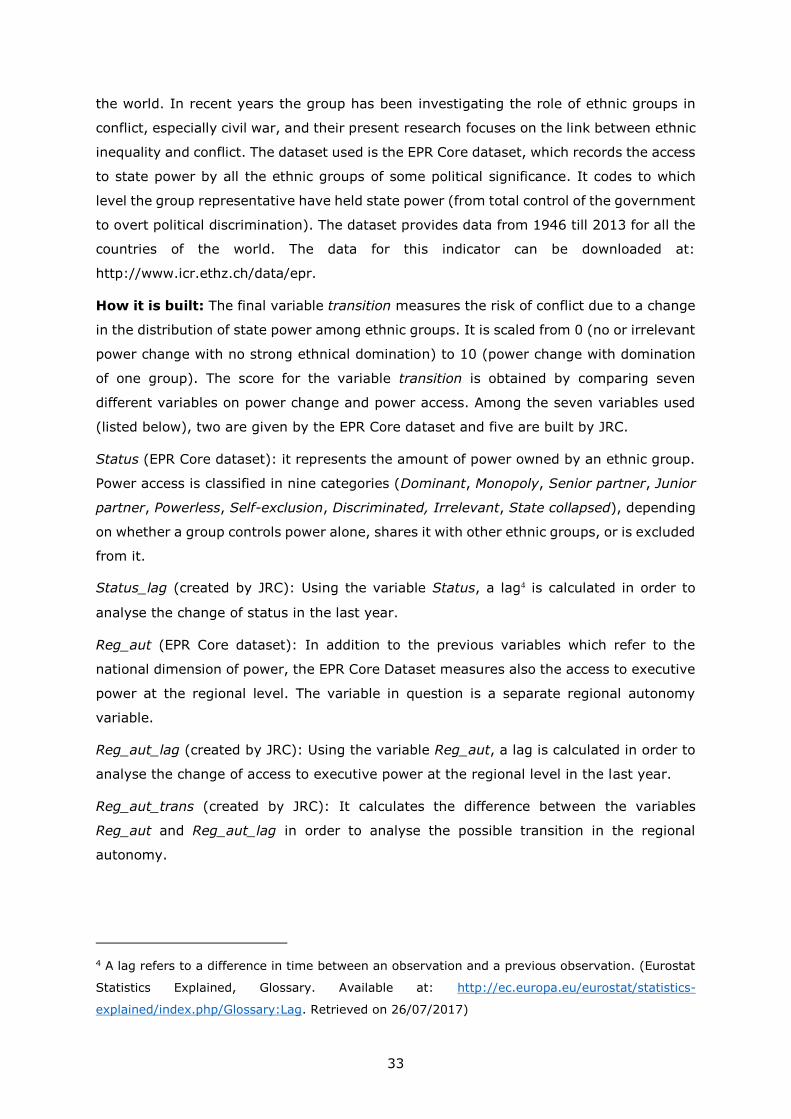
36
REG_AUT_TRANS
STATUS_LAG
1
IRRELEVANT 6
POWERLESS 6
DISCRIMINATED 6
INCEXC
STATUS
INC EXC
DOMINANT - 9
MONOPOLY - 9
IRRELEVANT 0 1
SENIOR PARTNER - 7
JUNIOR PARTNER - 7
DISCRIMINATION 3 -
SELF-EXCLUSION 1 -
POWERLESS 1 -
If the Incexc status is “included” and the regional autonomy scores 1, we assign 1.
In some cases, no comparisons are performed. If status is STATE COLLAPSED, then it is
coded as 10. If STATUS is IRRELEVANT, then we have 0 (zero). If status_lag is STATE
COLLAPSED, then we have 0 (zero).
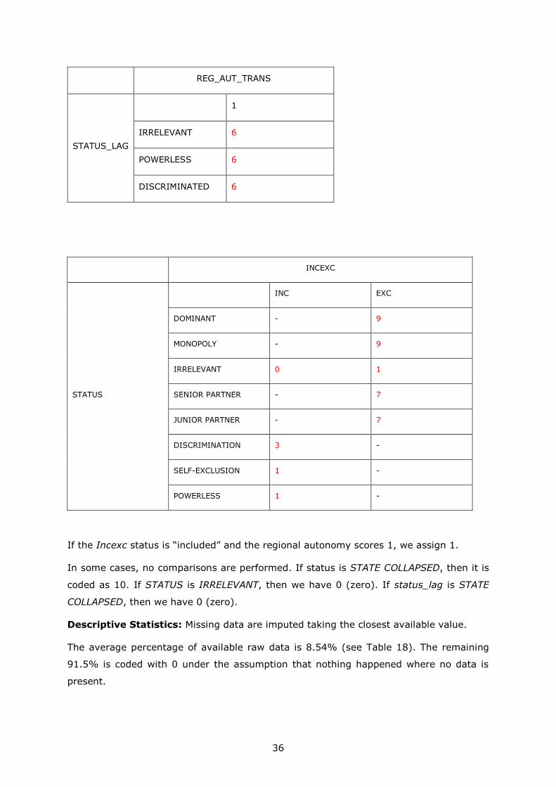
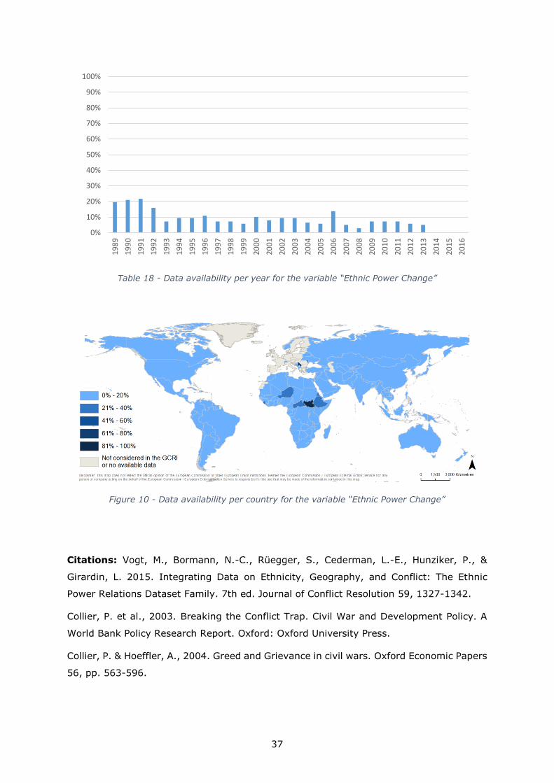
Descriptive Statistics: Missing data are imputed taking the closest available value.
The average percentage of available raw data is 8.54% (see Table 18). The remaining
91.5% is coded with 0 under the assumption that nothing happened where no data is
present.
37
Table 18 - Data availability per year for the variable “Ethnic Power Change”
Figure 10 - Data availability per country for the variable “Ethnic Power Change”
Citations: Vogt, M., Bormann, N.-C., Rüegger, S., Cederman, L.-E., Hunziker, P., &
Girardin, L. 2015. Integrating Data on Ethnicity, Geography, and Conflict: The Ethnic
Power Relations Dataset Family. 7th ed. Journal of Conflict Resolution 59, 1327-1342.
Collier, P. et al., 2003. Breaking the Conflict Trap. Civil War and Development Policy. A
World Bank Policy Research Report. Oxford: Oxford University Press.
Collier, P. & Hoeffler, A., 2004. Greed and Grievance in civil wars. Oxford Economic Papers
56, pp. 563-596.
0%
10%
20%
30%
40%
50%
60%
70%
80%
90%
100%
19
89
19
90
19
91
19
92
19
93
19
94
19
95
19
96
19
97
19
98
19
99
20
00
20
01
20
02
20
03
20
04
20
05
20
06
20
07
20
08
20
09
20
10
20
11
20
12
20
13
20
14
20
15
20
16

38
Wimmer, A., Cederman, L.-E. & Min, B., 2009. Ethnic Polictics and Armed Conflict: A
Configurational Analysis of a New Global Data Set. American Sociological Review, pp. 316-
337.
Reynal-Querol, M., 2002. Ethnicity, Political Systems, and Civil Wars, Sage Publications:
Journal of Conflict Resolution, Vol. 46, pp. 29-54.
3.11. Ethnic Compilation (ETHNIC_SN)
Description: If a country presents a very unbalanced distribution of power among ethnic
groups, then the political situation of that country is most likely not stable. The aim of
ethnic compilation is to measures how dangerous the unbalance of power between ethnic
groups can be.
Data source: This dataset is provided by the International Conflict Research (ICR) group
at ETH Zurich, as in 3.10 (please see above).
How it is built: The variable used is status which represents the amount of power owned
by an ethnic group. Power access is classified in nine categories (Dominant, Monopoly,
Senior partner, Junior partner, Powerless, Self-exclusion, Discriminated, Irrelevant, State
collapsed), depending on whether a group controls power alone, shares it with other ethnic
groups, or is excluded from it. We create a numerical classification of the variable as shown
in the table below.
STATUS SCORE
State collapse 10
Self-exclusion 9
Regional autonomy 7
Discriminated 5
Junior/Senior partner 5
Dominant/Monopoly 1
Powerless/Irrelevant 1
Table 19 - Ethnic compilation score
39
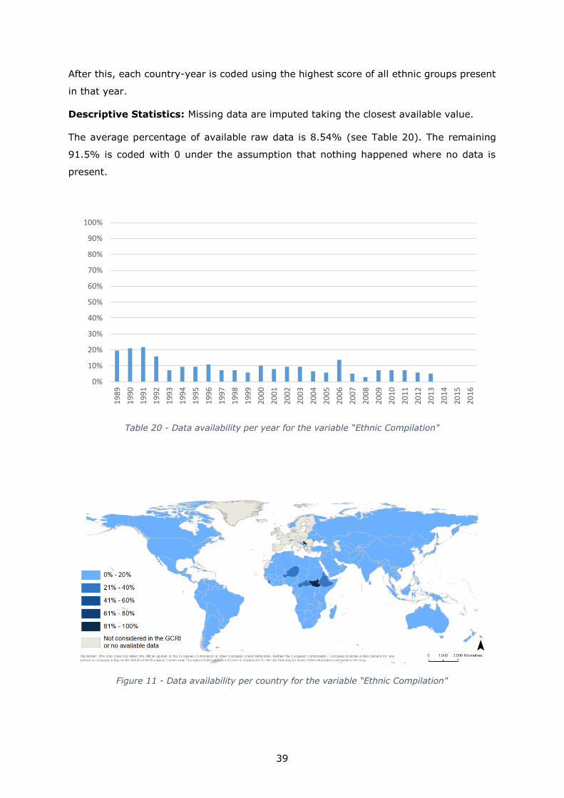
After this, each country-year is coded using the highest score of all ethnic groups present
in that year.
Descriptive Statistics: Missing data are imputed taking the closest available value.
The average percentage of available raw data is 8.54% (see Table 20). The remaining
91.5% is coded with 0 under the assumption that nothing happened where no data is
present.
Table 20 - Data availability per year for the variable “Ethnic Compilation"
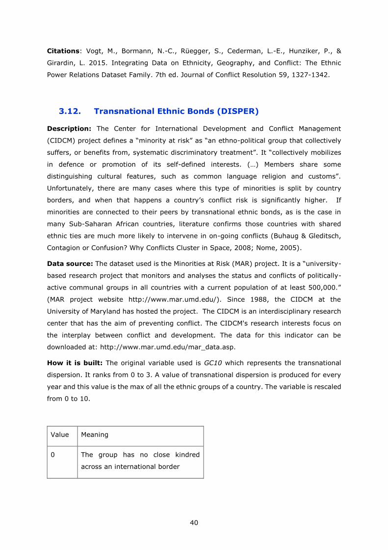
Figure 11 - Data availability per country for the variable “Ethnic Compilation"
0%
10%
20%
30%
40%
50%
60%
70%
80%
90%
100%
19
89
19
90
19
91
19
92
19
93
19
94
19
95
19
96
19
97
19
98
19
99
20
00
20
01
20
02
20
03
20
04
20
05
20
06
20
07
20
08
20
09
20
10
20
11
20
12
20
13
20
14
20
15
20
16
40
Citations: Vogt, M., Bormann, N.-C., Rüegger, S., Cederman, L.-E., Hunziker, P., &
Girardin, L. 2015. Integrating Data on Ethnicity, Geography, and Conflict: The Ethnic
Power Relations Dataset Family. 7th ed. Journal of Conflict Resolution 59, 1327-1342.
3.12. Transnational Ethnic Bonds (DISPER)
Description: The Center for International Development and Conflict Management
(CIDCM) project defines a “minority at risk” as “an ethno-political group that collectively
suffers, or benefits from, systematic discriminatory treatment”. It “collectively mobilizes
in defence or promotion of its self-defined interests. (…) Members share some
distinguishing cultural features, such as common language religion and customs”.
Unfortunately, there are many cases where this type of minorities is split by country
borders, and when that happens a country’s conflict risk is significantly higher. If
minorities are connected to their peers by transnational ethnic bonds, as is the case in
many Sub-Saharan African countries, literature confirms those countries with shared
ethnic ties are much more likely to intervene in on-going conflicts (Buhaug & Gleditsch,
Contagion or Confusion? Why Conflicts Cluster in Space, 2008; Nome, 2005).
Data source: The dataset used is the Minorities at Risk (MAR) project. It is a “university-
based research project that monitors and analyses the status and conflicts of politically-
active communal groups in all countries with a current population of at least 500,000.”
(MAR project website http://www.mar.umd.edu/). Since 1988, the CIDCM at the
University of Maryland has hosted the project. The CIDCM is an interdisciplinary research
center that has the aim of preventing conflict. The CIDCM's research interests focus on
the interplay between conflict and development. The data for this indicator can be
downloaded at: http://www.mar.umd.edu/mar_data.asp.
How it is built: The original variable used is GC10 which represents the transnational
dispersion. It ranks from 0 to 3. A value of transnational dispersion is produced for every
year and this value is the max of all the ethnic groups of a country. The variable is rescaled
from 0 to 10.
Value Meaning
0 The group has no close kindred
across an international border
41
1 The group has close kindred across
a border which does not adjoin its
regional base
2 The group has close kindred in one
country which adjoins its regional
base
3 The group has close kindred in more
than one country which adjoins its
regional base
Source: Minority at Risk Project (Available at:
http://www.mar.umd.edu/data/mar_codebook_Feb09.pdf)
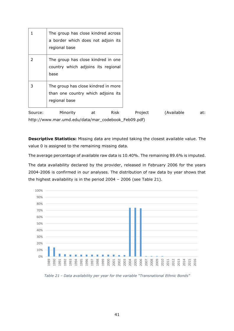
Descriptive Statistics: Missing data are imputed taking the closest available value. The
value 0 is assigned to the remaining missing data.
The average percentage of available raw data is 10.40%. The remaining 89.6% is imputed.
The data availability declared by the provider, released in February 2006 for the years
2004-2006 is confirmed in our analyses. The distribution of raw data by year shows that
the highest availability is in the period 2004 – 2006 (see Table 21).
Table 21 - Data availability per year for the variable “Transnational Ethnic Bonds”
0%
10%
20%
30%
40%
50%
60%
70%
80%
90%
100%
19
89
19
90
19
91
19
92
19
93
19
94
19
95
19
96
19
97
19
98
19
99
20
00
20
01
20
02
20
03
20
04
20
05
20
06
20
07
20
08
20
09
20
10
20
11
20
12
20
13
20
14
20
15
20
16
42
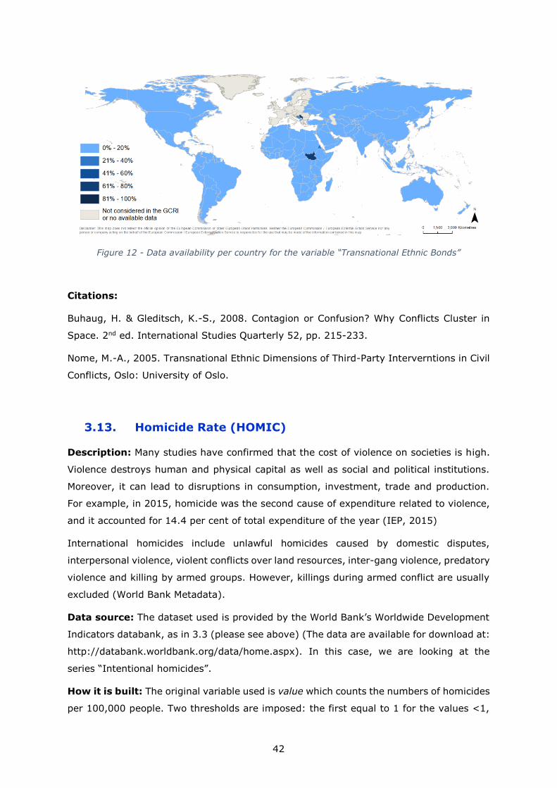
Figure 12 - Data availability per country for the variable “Transnational Ethnic Bonds”
Citations:
Buhaug, H. & Gleditsch, K.-S., 2008. Contagion or Confusion? Why Conflicts Cluster in
Space. 2nd ed. International Studies Quarterly 52, pp. 215-233.
Nome, M.-A., 2005. Transnational Ethnic Dimensions of Third-Party Interverntions in Civil
Conflicts, Oslo: University of Oslo.
3.13. Homicide Rate (HOMIC)
Description: Many studies have confirmed that the cost of violence on societies is high.
Violence destroys human and physical capital as well as social and political institutions.
Moreover, it can lead to disruptions in consumption, investment, trade and production.
For example, in 2015, homicide was the second cause of expenditure related to violence,
and it accounted for 14.4 per cent of total expenditure of the year (IEP, 2015)
International homicides include unlawful homicides caused by domestic disputes,
interpersonal violence, violent conflicts over land resources, inter-gang violence, predatory
violence and killing by armed groups. However, killings during armed conflict are usually
excluded (World Bank Metadata).
Data source: The dataset used is provided by the World Bank’s Worldwide Development
Indicators databank, as in 3.3 (please see above) (The data are available for download at:
http://databank.worldbank.org/data/home.aspx). In this case, we are looking at the
series “Intentional homicides”.
How it is built: The original variable used is value which counts the numbers of homicides
per 100,000 people. Two thresholds are imposed: the first equal to 1 for the values <1,
43
the second equal to 50 for the values >50. Then a log is applied to the distribution in order
to expand the low values and to shrink the high ones5. Two rescaling procedures are
performed the first with a min of 0 and a max of 30, the second with a min of 0 and a max
of 10.
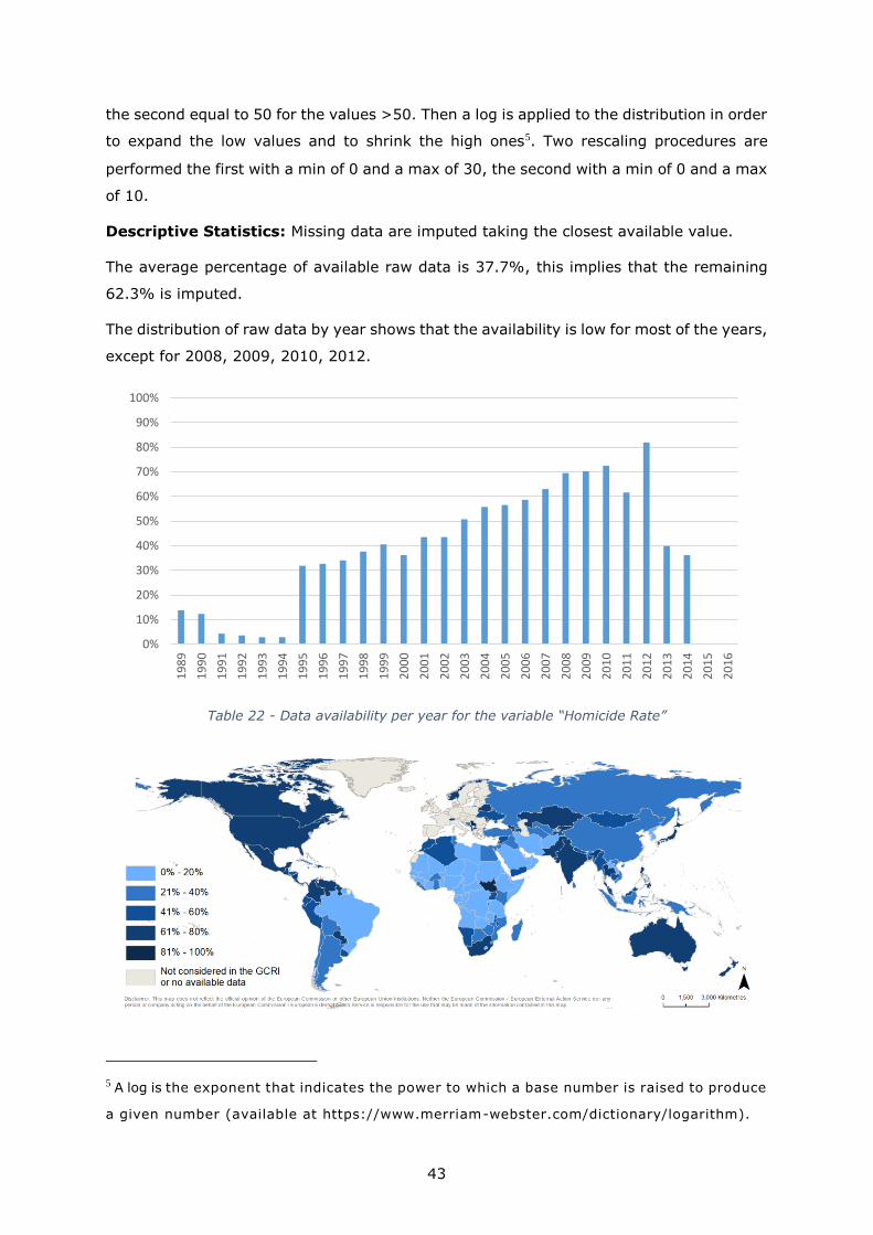
Descriptive Statistics: Missing data are imputed taking the closest available value.
The average percentage of available raw data is 37.7%, this implies that the remaining
62.3% is imputed.
The distribution of raw data by year shows that the availability is low for most of the years,
except for 2008, 2009, 2010, 2012.
Table 22 - Data availability per year for the variable “Homicide Rate”
5 A log is the exponent that indicates the power to which a base number is raised to produce
a given number (available at https://www.merriam-webster.com/dictionary/logarithm).
0%
10%
20%
30%
40%
50%
60%
70%
80%
90%
100%
19
89
19
90
19
91
19
92
19
93
19
94
19
95
19
96
19
97
19
98
19
99
20
00
20
01
20
02
20
03
20
04
20
05
20
06
20
07
20
08
20
09
20
10
20
11
20
12
20
13
20
14
20
15
20
16

44
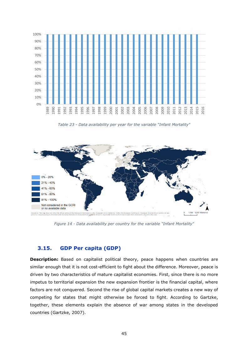
Figure 13 - Data availability per country for the variable “Homicide Rate”
Citations: IEP, 2015, Global Peace Index: measuring peace, its causes and its economic
value.
3.14. Infant Mortality (MORT)
Description: Two of the most frequently used indicators to evaluate the socioeconomic
progress or failure of a country are the life expectancy at birth and the survival to a certain
age. Both indicators provide a clear picture of how good the health system is, while the
under-five mortality captures also the effect of gender discrimination. Malnutrition and
medical services have a significant impact to this age group, and when female mortality
is higher, girls are likely to have less access to resources than boys (World Bank Metadata).
Data source: The dataset used is provided by the World Bank’s Worldwide Development
Indicators databank, as in 3.3 (please see above) (The data are available for download at:
http://databank.worldbank.org/data/home.aspx). In this case we are using the series
“Mortality rate, under-5 (per 1000 live births)”.
How it is built: The original variable used is SH.DYN.MORT which is the "under-five"
mortality rate. It measures the probability per 1,000 inhabitants that a newborn baby will
die before reaching the age of five, if subject to age-specific mortality rates of the specified
year. A log is firstly applied to the distribution and two rescaling procedures are then
performed: the first one with a minimum value of 0 and a maximum value of 130; and
the second one with a minimum value of 0 and a maximal value of 10.
Descriptive Statistics: Missing data are imputed taking the closest available value.
The average percentage of available raw data is 96.4%. The remaining 3.6% is imputed.
The distribution of raw data by year shows a very high availability of data.
45
Table 23 - Data availability per year for the variable “Infant Mortality"
Figure 14 - Data availability per country for the variable “Infant Mortality"
3.15. GDP Per capita (GDP)
Description: Based on capitalist political theory, peace happens when countries are
similar enough that it is not cost-efficient to fight about the difference. Moreover, peace is
driven by two characteristics of mature capitalist economies. First, since there is no more
impetus to territorial expansion the new expansion frontier is the financial capital, where
factors are not conquered. Second the rise of global capital markets creates a new way of
competing for states that might otherwise be forced to fight. According to Gartzke,
together, these elements explain the absence of war among states in the developed
countries (Gartzke, 2007).
0%
10%
20%
30%
40%
50%
60%
70%
80%
90%
100%
19
89
19
90
19
91
19
92
19
93
19
94
19
95
19
96
19
97
19
98
19
99
20
00
20
01
20
02
20
03
20
04
20
05
20
06
20
07
20
08
20
09
20
10
20
11
20
12
20
13
20
14
20
15
20
16
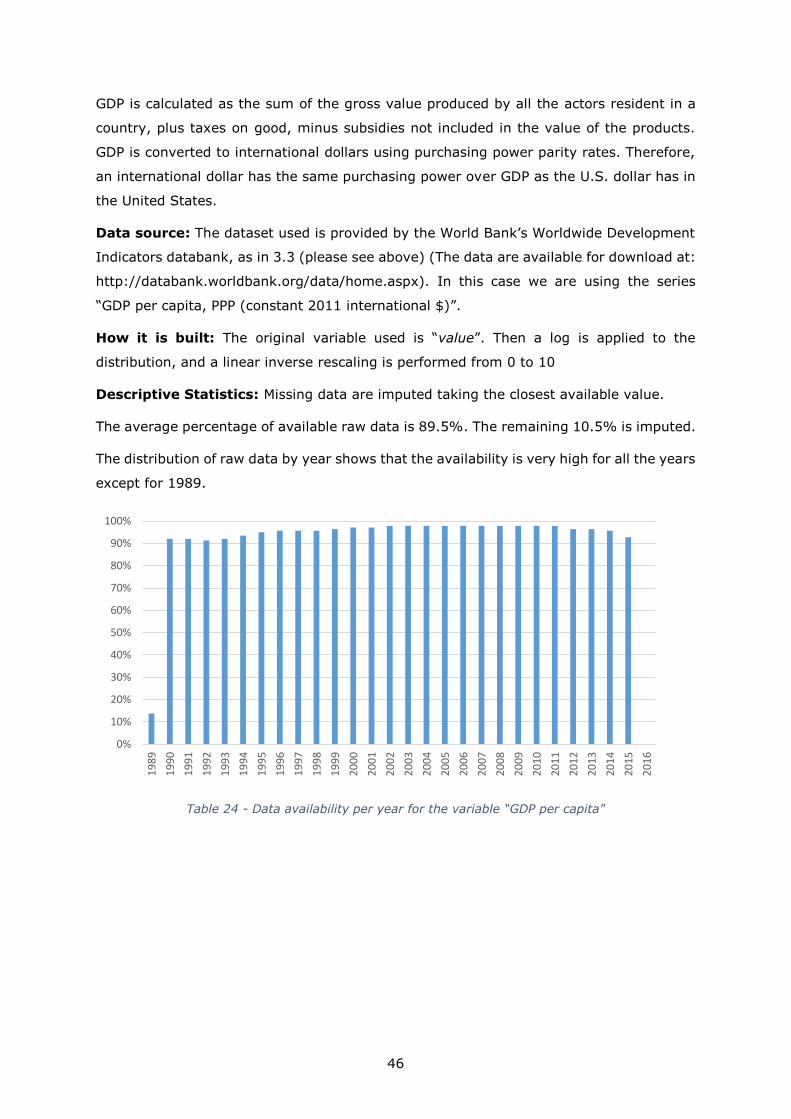
46
GDP is calculated as the sum of the gross value produced by all the actors resident in a
country, plus taxes on good, minus subsidies not included in the value of the products.
GDP is converted to international dollars using purchasing power parity rates. Therefore,
an international dollar has the same purchasing power over GDP as the U.S. dollar has in
the United States.
Data source: The dataset used is provided by the World Bank’s Worldwide Development
Indicators databank, as in 3.3 (please see above) (The data are available for download at:
http://databank.worldbank.org/data/home.aspx). In this case we are using the series
“GDP per capita, PPP (constant 2011 international $)”.
How it is built: The original variable used is “value”. Then a log is applied to the
distribution, and a linear inverse rescaling is performed from 0 to 10
Descriptive Statistics: Missing data are imputed taking the closest available value.
The average percentage of available raw data is 89.5%. The remaining 10.5% is imputed.
The distribution of raw data by year shows that the availability is very high for all the years
except for 1989.
Table 24 - Data availability per year for the variable “GDP per capita"
0%
10%
20%
30%
40%
50%
60%
70%
80%
90%
100%
19
89
19
90
19
91
19
92
19
93
19
94
19
95
19
96
19
97
19
98
19
99
20
00
20
01
20
02
20
03
20
04
20
05
20
06
20
07
20
08
20
09
20
10
20
11
20
12
20
13
20
14
20
15
20
16
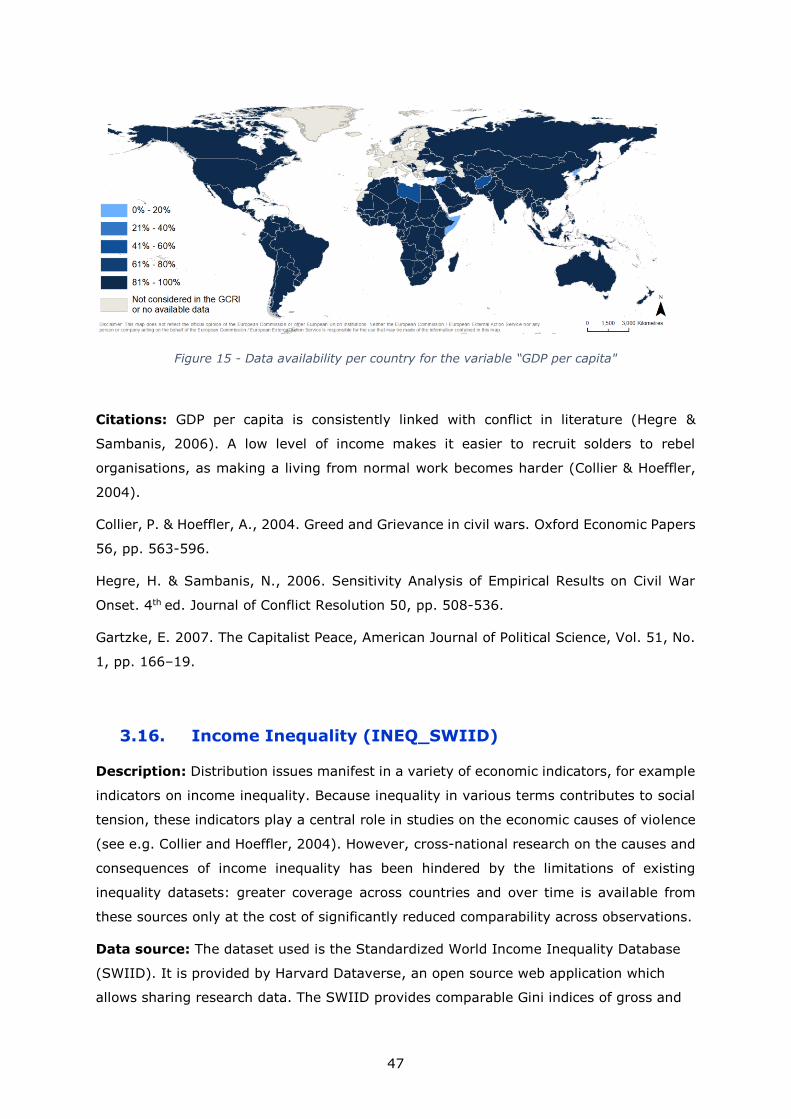
47
Figure 15 - Data availability per country for the variable “GDP per capita"
Citations: GDP per capita is consistently linked with conflict in literature (Hegre &
Sambanis, 2006). A low level of income makes it easier to recruit solders to rebel
organisations, as making a living from normal work becomes harder (Collier & Hoeffler,
2004).
Collier, P. & Hoeffler, A., 2004. Greed and Grievance in civil wars. Oxford Economic Papers
56, pp. 563-596.
Hegre, H. & Sambanis, N., 2006. Sensitivity Analysis of Empirical Results on Civil War
Onset. 4th ed. Journal of Conflict Resolution 50, pp. 508-536.
Gartzke, E. 2007. The Capitalist Peace, American Journal of Political Science, Vol. 51, No.
1, pp. 166–19.
3.16. Income Inequality (INEQ_SWIID)
Description: Distribution issues manifest in a variety of economic indicators, for example
indicators on income inequality. Because inequality in various terms contributes to social
tension, these indicators play a central role in studies on the economic causes of violence
(see e.g. Collier and Hoeffler, 2004). However, cross-national research on the causes and
consequences of income inequality has been hindered by the limitations of existing
inequality datasets: greater coverage across countries and over time is available from
these sources only at the cost of significantly reduced comparability across observations.
Data source: The dataset used is the Standardized World Income Inequality Database
(SWIID). It is provided by Harvard Dataverse, an open source web application which
allows sharing research data. The SWIID provides comparable Gini indices of gross and
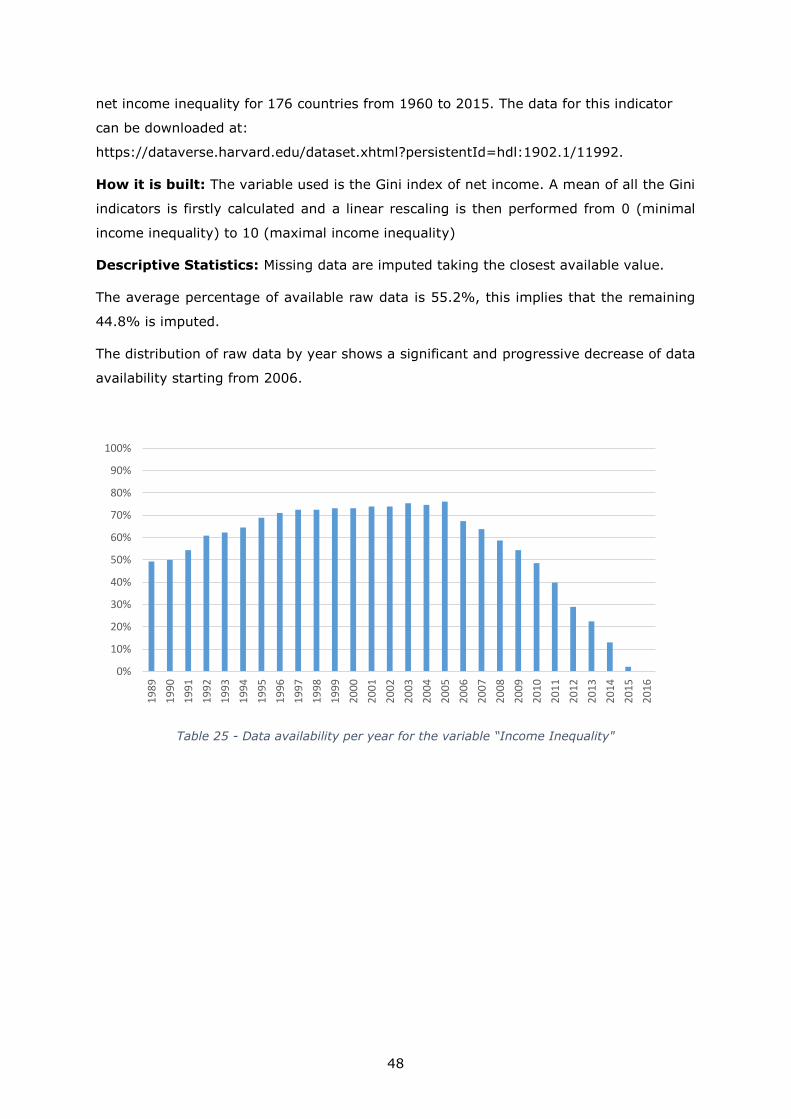
48
net income inequality for 176 countries from 1960 to 2015. The data for this indicator
can be downloaded at:
https://dataverse.harvard.edu/dataset.xhtml?persistentId=hdl:1902.1/11992.
How it is built: The variable used is the Gini index of net income. A mean of all the Gini
indicators is firstly calculated and a linear rescaling is then performed from 0 (minimal
income inequality) to 10 (maximal income inequality)
Descriptive Statistics: Missing data are imputed taking the closest available value.
The average percentage of available raw data is 55.2%, this implies that the remaining
44.8% is imputed.
The distribution of raw data by year shows a significant and progressive decrease of data
availability starting from 2006.
Table 25 - Data availability per year for the variable “Income Inequality"
0%
10%
20%
30%
40%
50%
60%
70%
80%
90%
100%
19
89
19
90
19
91
19
92
19
93
19
94
19
95
19
96
19
97
19
98
19
99
20
00
20
01
20
02
20
03
20
04
20
05
20
06
20
07
20
08
20
09
20
10
20
11
20
12
20
13
20
14
20
15
20
16
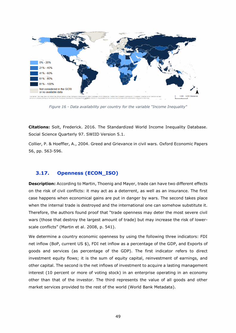
49
Figure 16 - Data availability per country for the variable “Income Inequality"
Citations: Solt, Frederick. 2016. The Standardized World Income Inequality Database.
Social Science Quarterly 97. SWIID Version 5.1.
Collier, P. & Hoeffler, A., 2004. Greed and Grievance in civil wars. Oxford Economic Papers
56, pp. 563-596.
3.17. Openness (ECON_ISO)
Description: According to Martin, Thoenig and Mayer, trade can have two different effects
on the risk of civil conflicts: it may act as a deterrent, as well as an insurance. The first
case happens when economical gains are put in danger by wars. The second takes place
when the internal trade is destroyed and the international one can somehow substitute it.
Therefore, the authors found proof that “trade openness may deter the most severe civil
wars (those that destroy the largest amount of trade) but may increase the risk of lower-
scale conflicts” (Martin et al. 2008, p. 541).
We determine a country economic openness by using the following three indicators: FDI
net inflow (BoP, current US $), FDI net inflow as a percentage of the GDP, and Exports of
goods and services (as percentage of the GDP). The first indicator refers to direct
investment equity flows; it is the sum of equity capital, reinvestment of earnings, and
other capital. The second is the net inflows of investment to acquire a lasting management
interest (10 percent or more of voting stock) in an enterprise operating in an economy
other than that of the investor. The third represents the value of all goods and other
market services provided to the rest of the world (World Bank Metadata).
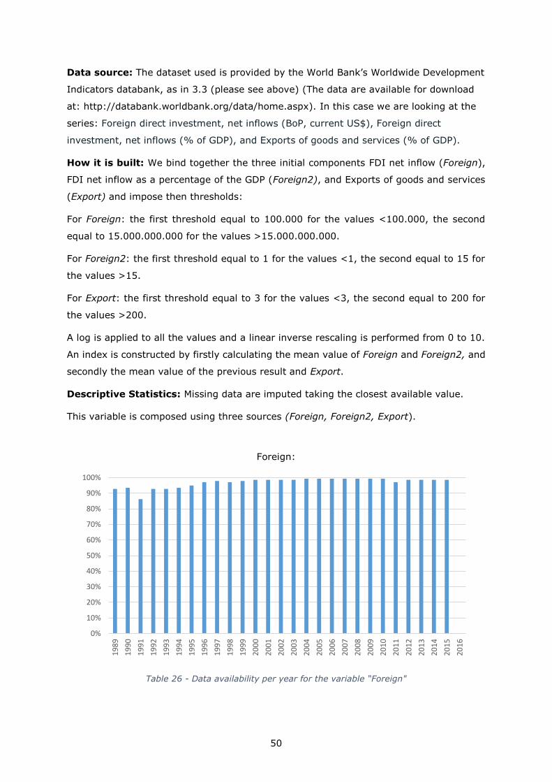
50
Data source: The dataset used is provided by the World Bank’s Worldwide Development
Indicators databank, as in 3.3 (please see above) (The data are available for download
at: http://databank.worldbank.org/data/home.aspx). In this case we are looking at the
series: Foreign direct investment, net inflows (BoP, current US$), Foreign direct
investment, net inflows (% of GDP), and Exports of goods and services (% of GDP).
How it is built: We bind together the three initial components FDI net inflow (Foreign),
FDI net inflow as a percentage of the GDP (Foreign2), and Exports of goods and services
(Export) and impose then thresholds:
For Foreign: the first threshold equal to 100.000 for the values <100.000, the second
equal to 15.000.000.000 for the values >15.000.000.000.
For Foreign2: the first threshold equal to 1 for the values <1, the second equal to 15 for
the values >15.
For Export: the first threshold equal to 3 for the values <3, the second equal to 200 for
the values >200.
A log is applied to all the values and a linear inverse rescaling is performed from 0 to 10.
An index is constructed by firstly calculating the mean value of Foreign and Foreign2, and
secondly the mean value of the previous result and Export.
Descriptive Statistics: Missing data are imputed taking the closest available value.
This variable is composed using three sources (Foreign, Foreign2, Export).
Foreign:
Table 26 - Data availability per year for the variable “Foreign"
0%
10%
20%
30%
40%
50%
60%
70%
80%
90%
100%
19
89
19
90
19
91
19
92
19
93
19
94
19
95
19
96
19
97
19
98
19
99
20
00
20
01
20
02
20
03
20
04
20
05
20
06
20
07
20
08
20
09
20
10
20
11
20
12
20
13
20
14
20
15
20
16

51
Figure 17 - Data availability per country for the variable “Foreign"
The average percentage of available raw data is 93.45%. The remaining 6.5% is imputed.
The distribution of raw data by year shows a complete availability of information in the
period 1989 – 2015.
Foreign2:
Table 27 - Data availability per year for the variable “Foreign2"
0%
10%
20%
30%
40%
50%
60%
70%
80%
90%
100%
19
89
19
90
19
91
19
92
19
93
19
94
19
95
19
96
19
97
19
98
19
99
20
00
20
01
20
02
20
03
20
04
20
05
20
06
20
07
20
08
20
09
20
10
20
11
20
12
20
13
20
14
20
15
20
16
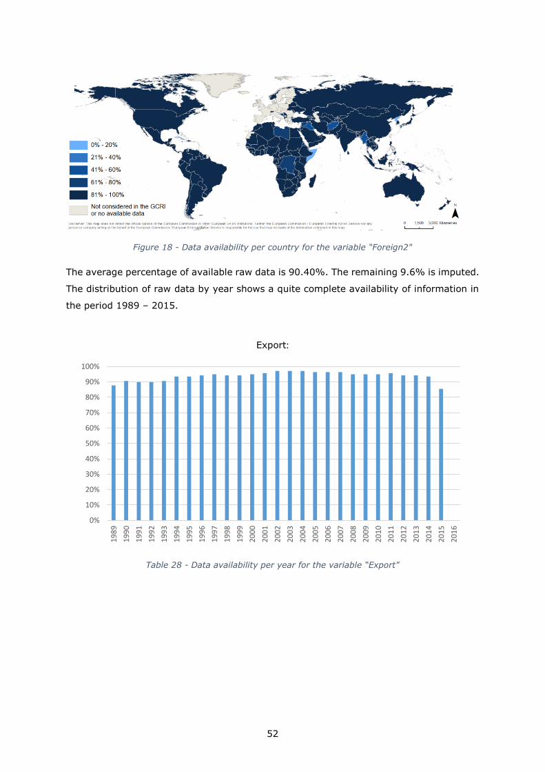
52
Figure 18 - Data availability per country for the variable “Foreign2"
The average percentage of available raw data is 90.40%. The remaining 9.6% is imputed.
The distribution of raw data by year shows a quite complete availability of information in
the period 1989 – 2015.
Export:
Table 28 - Data availability per year for the variable “Export"
0%
10%
20%
30%
40%
50%
60%
70%
80%
90%
100%
19
89
19
90
19
91
19
92
19
93
19
94
19
95
19
96
19
97
19
98
19
99
20
00
20
01
20
02
20
03
20
04
20
05
20
06
20
07
20
08
20
09
20
10
20
11
20
12
20
13
20
14
20
15
20
16
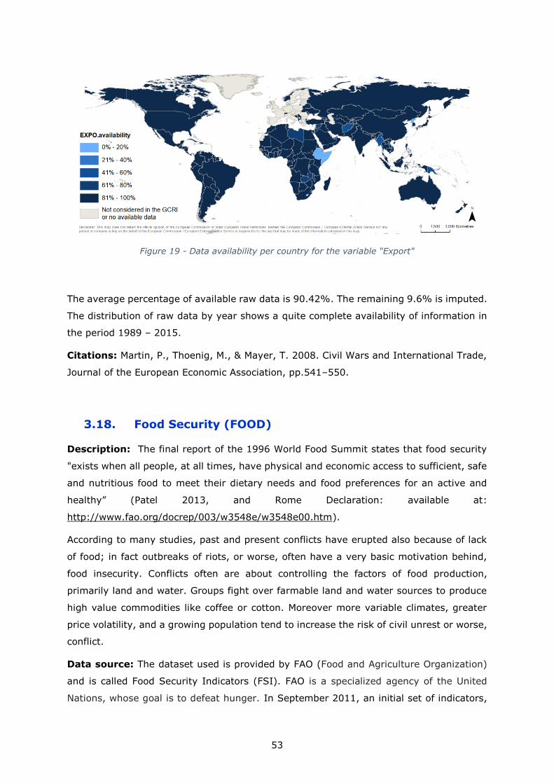
53
Figure 19 - Data availability per country for the variable “Export"
The average percentage of available raw data is 90.42%. The remaining 9.6% is imputed.
The distribution of raw data by year shows a quite complete availability of information in
the period 1989 – 2015.
Citations: Martin, P., Thoenig, M., & Mayer, T. 2008. Civil Wars and International Trade,
Journal of the European Economic Association, pp.541–550.
3.18. Food Security (FOOD)
Description: The final report of the 1996 World Food Summit states that food security
"exists when all people, at all times, have physical and economic access to sufficient, safe
and nutritious food to meet their dietary needs and food preferences for an active and
healthy” (Patel 2013, and Rome Declaration: available at:
http://www.fao.org/docrep/003/w3548e/w3548e00.htm).
According to many studies, past and present conflicts have erupted also because of lack
of food; in fact outbreaks of riots, or worse, often have a very basic motivation behind,
food insecurity. Conflicts often are about controlling the factors of food production,
primarily land and water. Groups fight over farmable land and water sources to produce
high value commodities like coffee or cotton. Moreover more variable climates, greater
price volatility, and a growing population tend to increase the risk of civil unrest or worse,
conflict.
Data source: The dataset used is provided by FAO (Food and Agriculture Organization)
and is called Food Security Indicators (FSI). FAO is a specialized agency of the United
Nations, whose goal is to defeat hunger. In September 2011, an initial set of indicators,
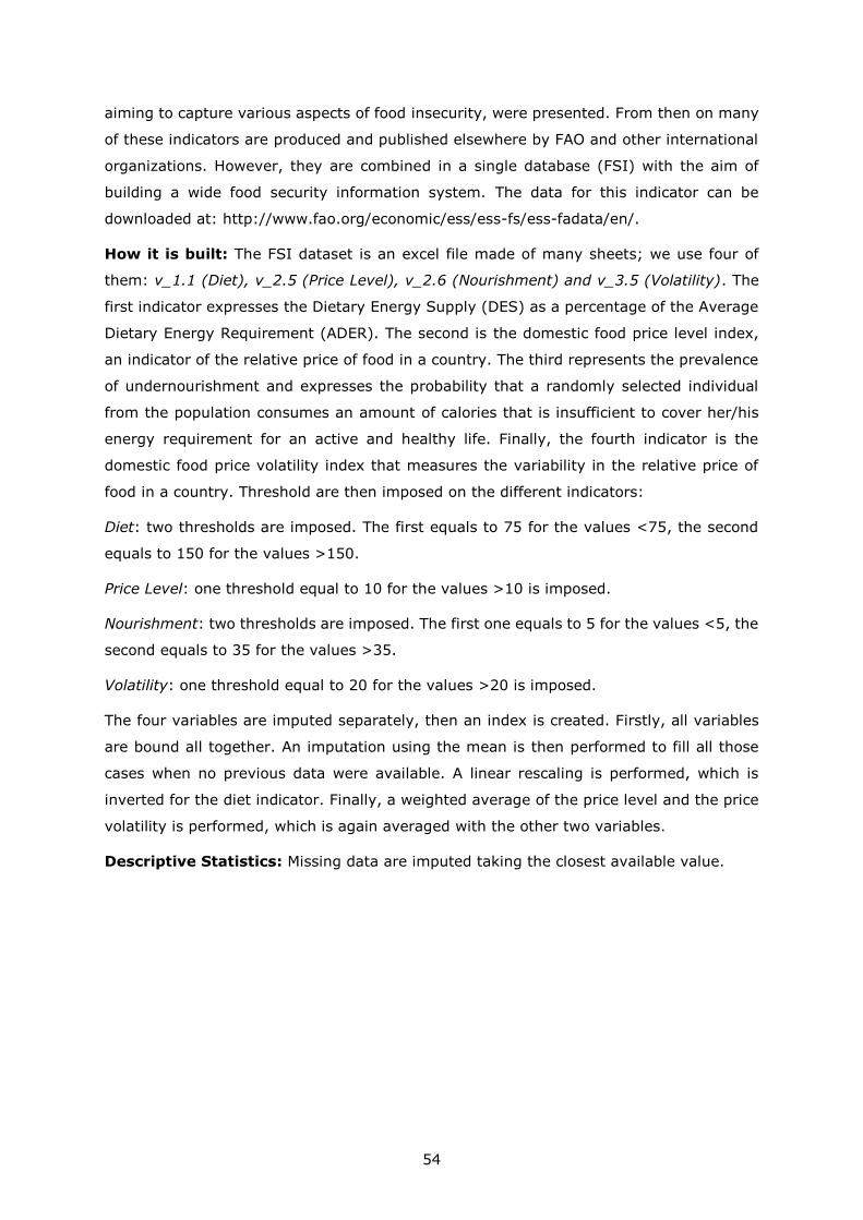
54
aiming to capture various aspects of food insecurity, were presented. From then on many
of these indicators are produced and published elsewhere by FAO and other international
organizations. However, they are combined in a single database (FSI) with the aim of
building a wide food security information system. The data for this indicator can be
downloaded at: http://www.fao.org/economic/ess/ess-fs/ess-fadata/en/.
How it is built: The FSI dataset is an excel file made of many sheets; we use four of
them: v_1.1 (Diet), v_2.5 (Price Level), v_2.6 (Nourishment) and v_3.5 (Volatility). The
first indicator expresses the Dietary Energy Supply (DES) as a percentage of the Average
Dietary Energy Requirement (ADER). The second is the domestic food price level index,
an indicator of the relative price of food in a country. The third represents the prevalence
of undernourishment and expresses the probability that a randomly selected individual
from the population consumes an amount of calories that is insufficient to cover her/his
energy requirement for an active and healthy life. Finally, the fourth indicator is the
domestic food price volatility index that measures the variability in the relative price of
food in a country. Threshold are then imposed on the different indicators:
Diet: two thresholds are imposed. The first equals to 75 for the values <75, the second
equals to 150 for the values >150.
Price Level: one threshold equal to 10 for the values >10 is imposed.
Nourishment: two thresholds are imposed. The first one equals to 5 for the values <5, the
second equals to 35 for the values >35.
Volatility: one threshold equal to 20 for the values >20 is imposed.
The four variables are imputed separately, then an index is created. Firstly, all variables
are bound all together. An imputation using the mean is then performed to fill all those
cases when no previous data were available. A linear rescaling is performed, which is
inverted for the diet indicator. Finally, a weighted average of the price level and the price
volatility is performed, which is again averaged with the other two variables.
Descriptive Statistics: Missing data are imputed taking the closest available value.
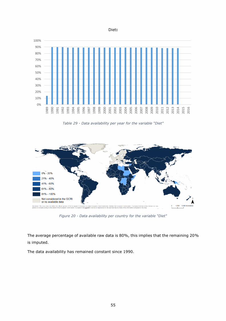
55
Diet:
Table 29 - Data availability per year for the variable “Diet"
Figure 20 - Data availability per country for the variable “Diet"
The average percentage of available raw data is 80%, this implies that the remaining 20%
is imputed.
The data availability has remained constant since 1990.
0%
10%
20%
30%
40%
50%
60%
70%
80%
90%
100%
19
89
19
90
19
91
19
92
19
93
19
94
19
95
19
96
19
97
19
98
19
99
20
00
20
01
20
02
20
03
20
04
20
05
20
06
20
07
20
08
20
09
20
10
20
11
20
12
20
13
20
14
20
15
20
16

56
Price Level:
Table 30 - Data availability per year for the variable “Price Level"
Figure 21 - Data availability per country for the variable “Price Level"
The average percentage of available raw data is 76%. The remaining 24% is imputed.
The data availability has remained constant during the years.
0%
10%
20%
30%
40%
50%
60%
70%
80%
90%
100%
19
89
19
90
19
91
19
92
19
93
19
94
19
95
19
96
19
97
19
98
19
99
20
00
20
01
20
02
20
03
20
04
20
05
20
06
20
07
20
08
20
09
20
10
20
11
20
12
20
13
20
14
20
15
20
16
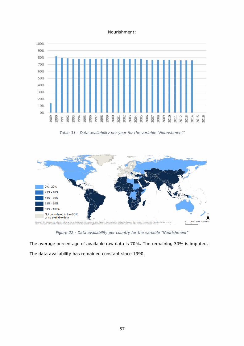
57
Nourishment:
Table 31 - Data availability per year for the variable “Nourishment"
Figure 22 - Data availability per country for the variable “Nourishment"
The average percentage of available raw data is 70%. The remaining 30% is imputed.
The data availability has remained constant since 1990.
0%
10%
20%
30%
40%
50%
60%
70%
80%
90%
100%
19
89
19
90
19
91
19
92
19
93
19
94
19
95
19
96
19
97
19
98
19
99
20
00
20
01
20
02
20
03
20
04
20
05
20
06
20
07
20
08
20
09
20
10
20
11
20
12
20
13
20
14
20
15
20
16

58
Volatility:
Table 32 - Data availability per year for the variable “Volatility"
Figure 23 - Data availability per country for the variable “Volatility"
The average percentage of available raw data is 40.1%. The remaining 59.9% is imputed.
The data availability is very poor until 2000. from 2001 until 2014 it improves sensibly.
Citations: FAO, UN. 2003. Trade Reforms and Food Security: Conceptualizing the
Linkages.
Patel, P. 2013. Food sovereignty is next big idea. Financial Times.
FAO, UN. 1996. Rome Declaration on Food Security and World Food Summit Plan of Action.
0%
10%
20%
30%
40%
50%
60%
70%
80%
90%
100%
19
89
19
90
19
91
19
92
19
93
19
94
19
95
19
96
19
97
19
98
19
99
20
00
20
01
20
02
20
03
20
04
20
05
20
06
20
07
20
08
20
09
20
10
20
11
20
12
20
13
20
14
20
15
20
16

59
Bora, S., Ceccacci, I., Delgado, C., & Townsend. R. 2010. Food security and Conflict, World
Bank: World Development Report 2011.
3.19. Unemployment (UNEMP)
Description: Unemployment is a key measure to monitor whether a country is
implementing policies for an inclusive economic growth and for full employment. What has
been noted is that low unemployment rates can disguise substantial poverty in a country,
while high unemployment rates can occur in countries highly economically developed. This
happens because if workers can rely on unemployment benefits and on a safety net, then
they can wait for suitable jobs. While in poor countries with no state support, citizens
accept jobs even if underpaid or unsafe.
Unemployed are those individuals without work, but that have been searching for a job in
a recent past period, and that are currently available for work. Persons who, although are
not looking for work, have an arrangement for a future job are also considered
unemployed. A certain unemployment level is unavoidable, also just because workers
change jobs and generally they are jobless in between. (World Bank Metadata).
Unemployment is considered a possible cause of recruiting members of insurgent groups,
gangs or even extremist cells, in fact, according to economic theories, unemployed people
have a low opportunity cost of engaging in violence and therefore low recruitment costs.
Data source: The dataset used is provided by the World Bank’s Worldwide Development
Indicators databank, as in 3.3 (please see above) (The data are available for download
at: http://databank.worldbank.org/data/home.aspx). In this case we are looking at the
series: Unemployment, total (% of total labour force).
How it is built: The variable used is value. A threshold equal to 2 has been imposed for
the values <2, then a linear rescaling is performed from 0 to 10.
Descriptive Statistics: Missing data are imputed taking the closest available value.
The average percentage of available raw data is 85.9%. The remaining 14.1% is imputed.
The distribution of raw data by year reports a very good data coverage since 1991, while
for the most part data for years 1989 and 1990, had to be imputed.
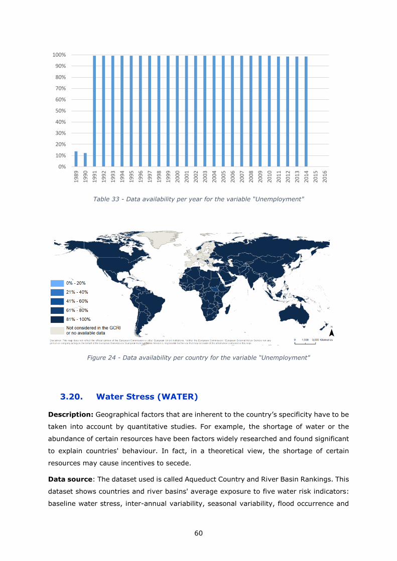
60
Table 33 - Data availability per year for the variable “Unemployment"
Figure 24 - Data availability per country for the variable “Unemployment"
3.20. Water Stress (WATER)
Description: Geographical factors that are inherent to the country’s specificity have to be
taken into account by quantitative studies. For example, the shortage of water or the
abundance of certain resources have been factors widely researched and found significant
to explain countries' behaviour. In fact, in a theoretical view, the shortage of certain
resources may cause incentives to secede.
Data source: The dataset used is called Aqueduct Country and River Basin Rankings. This
dataset shows countries and river basins' average exposure to five water risk indicators:
baseline water stress, inter-annual variability, seasonal variability, flood occurrence and
0%
10%
20%
30%
40%
50%
60%
70%
80%
90%
100%
19
89
19
90
19
91
19
92
19
93
19
94
19
95
19
96
19
97
19
98
19
99
20
00
20
01
20
02
20
03
20
04
20
05
20
06
20
07
20
08
20
09
20
10
20
11
20
12
20
13
20
14
20
15
20
16
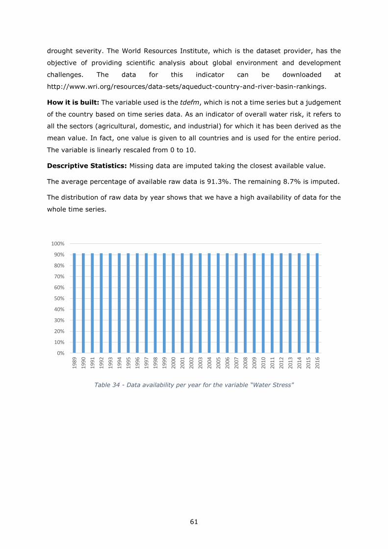
61
drought severity. The World Resources Institute, which is the dataset provider, has the
objective of providing scientific analysis about global environment and development
challenges. The data for this indicator can be downloaded at
http://www.wri.org/resources/data-sets/aqueduct-country-and-river-basin-rankings.
How it is built: The variable used is the tdefm, which is not a time series but a judgement
of the country based on time series data. As an indicator of overall water risk, it refers to
all the sectors (agricultural, domestic, and industrial) for which it has been derived as the
mean value. In fact, one value is given to all countries and is used for the entire period.
The variable is linearly rescaled from 0 to 10.
Descriptive Statistics: Missing data are imputed taking the closest available value.
The average percentage of available raw data is 91.3%. The remaining 8.7% is imputed.
The distribution of raw data by year shows that we have a high availability of data for the
whole time series.
Table 34 - Data availability per year for the variable “Water Stress"
0%
10%
20%
30%
40%
50%
60%
70%
80%
90%
100%
19
89
19
90
19
91
19
92
19
93
19
94
19
95
19
96
19
97
19
98
19
99
20
00
20
01
20
02
20
03
20
04
20
05
20
06
20
07
20
08
20
09
20
10
20
11
20
12
20
13
20
14
20
15
20
16

62
Figure 25 - Data availability per country for the variable “Water Stress"
Citations: Gassert, F., Reig, P., Luo, T., & Maddocks, A. 2013. Aqueduct country and river
basin rankings: a weighted aggregation of spatially distinct hydrological indicators.
Working paper. Washington, DC: World Resources Institute.
3.21. Oil Producer (FUEL_EXP)
Description: Several studies show that oil producers have a higher risk of conflict than
other countries, whereas the correlations for other resources and conflict are oftentimes
insignificant (Dixon, 2009). Indeed, based on a compilation of several quantitative
studies, Dixon shows a high degree of consensus on the increased vulnerability of oil
exporters to civil wars (2009).
Data source: The dataset used is provided by the World Bank’s Worldwide Development
Indicators databank, as in 3.3 (please see above) (The data are available for download at:
http://databank.worldbank.org/data/home.aspx). The World Bank measures fuels exports
for each country, where fuels comprise the commodities in SITC (Standard International
Trade Classification) section 3. We are looking at the series “Fuel exports (% of
merchandise exports)” in the databank “World Development Indicators”.
How it is built: The variable used is value which represents the fuel exports as percentage
of merchandise exports. A threshold equal to 1 is imposed for values <1. A log is then
applied to the distribution, which is linearly rescaled from 0 to 10.
Descriptive Statistics: Missing data are imputed taking the closest available value.
The average percentage of available raw data is 66.9%. The remaining 33.1% is imputed.
The data availability increased from 1992 to 2001, then it has remained quite stable.

63
Table 35 - Data availability per year for the variable “Oil Producer"
Figure 26 - Data availability per country for the variable “Oil Producer"
Citations: Dixon, J. 2009. What causes civil wars? Integrating Quantitative Research
Findings. International Studies Review 11, pp. 707-735.
3.22. Structural Constraints (STRUCT)
Description: Are countries in transition able to moderate and de-escalate conflict?
According to Hauke Hartmann6 this is still one of the main difficulties that transition
countries have to face. They still lack for the most part the ability to prevent conflict, and
“this has always made it more difficult for them to steer transformation processes (…).
6 Senior Project Manager at BTI
0%
10%
20%
30%
40%
50%
60%
70%
80%
90%
100%
19
89
19
90
19
91
19
92
19
93
19
94
19
95
19
96
19
97
19
98
19
99
20
00
20
01
20
02
20
03
20
04
20
05
20
06
20
07
20
08
20
09
20
10
20
11
20
12
20
13
20
14
20
15
20
16
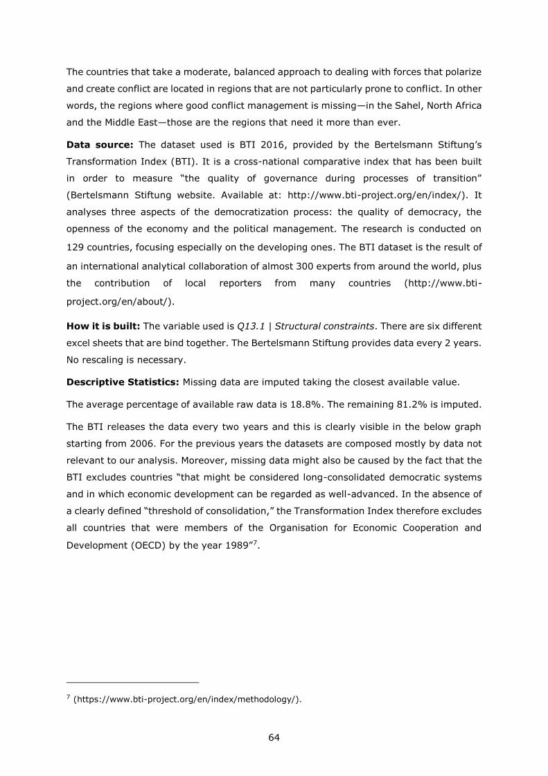
64
The countries that take a moderate, balanced approach to dealing with forces that polarize
and create conflict are located in regions that are not particularly prone to conflict. In other
words, the regions where good conflict management is missing—in the Sahel, North Africa
and the Middle East—those are the regions that need it more than ever.
Data source: The dataset used is BTI 2016, provided by the Bertelsmann Stiftung’s
Transformation Index (BTI). It is a cross-national comparative index that has been built
in order to measure “the quality of governance during processes of transition”
(Bertelsmann Stiftung website. Available at: http://www.bti-project.org/en/index/). It
analyses three aspects of the democratization process: the quality of democracy, the
openness of the economy and the political management. The research is conducted on
129 countries, focusing especially on the developing ones. The BTI dataset is the result of
an international analytical collaboration of almost 300 experts from around the world, plus
the contribution of local reporters from many countries (http://www.bti-
project.org/en/about/).
How it is built: The variable used is Q13.1 | Structural constraints. There are six different
excel sheets that are bind together. The Bertelsmann Stiftung provides data every 2 years.
No rescaling is necessary.
Descriptive Statistics: Missing data are imputed taking the closest available value.
The average percentage of available raw data is 18.8%. The remaining 81.2% is imputed.
The BTI releases the data every two years and this is clearly visible in the below graph
starting from 2006. For the previous years the datasets are composed mostly by data not
relevant to our analysis. Moreover, missing data might also be caused by the fact that the
BTI excludes countries “that might be considered long-consolidated democratic systems
and in which economic development can be regarded as well-advanced. In the absence of
a clearly defined “threshold of consolidation,” the Transformation Index therefore excludes
all countries that were members of the Organisation for Economic Cooperation and
Development (OECD) by the year 1989”7.
7 (https://www.bti-project.org/en/index/methodology/).
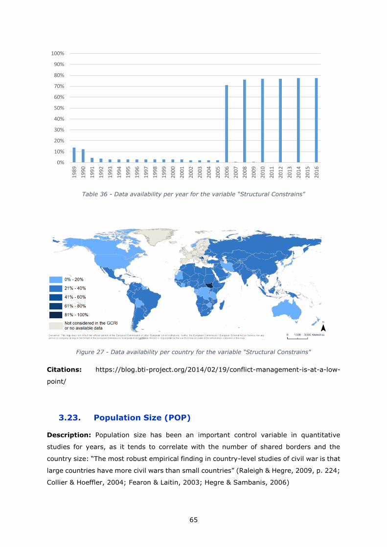
65
Table 36 - Data availability per year for the variable “Structural Constrains"
Figure 27 - Data availability per country for the variable “Structural Constrains"
Citations: https://blog.bti-project.org/2014/02/19/conflict-management-is-at-a-low-
point/
3.23. Population Size (POP)
Description: Population size has been an important control variable in quantitative
studies for years, as it tends to correlate with the number of shared borders and the
country size: “The most robust empirical finding in country-level studies of civil war is that
large countries have more civil wars than small countries” (Raleigh & Hegre, 2009, p. 224;
Collier & Hoeffler, 2004; Fearon & Laitin, 2003; Hegre & Sambanis, 2006)
0%
10%
20%
30%
40%
50%
60%
70%
80%
90%
100%
19
89
19
90
19
91
19
92
19
93
19
94
19
95
19
96
19
97
19
98
19
99
20
00
20
01
20
02
20
03
20
04
20
05
20
06
20
07
20
08
20
09
20
10
20
11
20
12
20
13
20
14
20
15
20
16

66
Data source: The dataset used is called “Annual Population by Age-both Sexes” and is
the twenty-fifth round of official United Nations population estimates and projections that
have been prepared by the Population Division of the Department of Economic and Social
Affairs of the United Nations Secretariat. The UN Population Division assists the
Department of Economic and Social Affairs in discharging its functions as member of the
Global Migration Group. The data for this indicator can be downloaded at:
http://esa.un.org/unpd/wpp/Download/Standard/Interpolated/.
How it is built: We sum the population, which is divided by age, in order to know the
total population of a country for a specific year. A log is firstly applied to the distribution.
Then, a threshold equal to 6 is imposed for values <6, and a threshold equal to 12.5 is
imposed for values <12.5. Finally, the values are rescaled from 0 to 10.
Descriptive Statistics: No missing data. The average percentage of available raw data
is 100%.
Table 37 - Data availability per year for the variable “Population Size"
0%
10%
20%
30%
40%
50%
60%
70%
80%
90%
100%
19
89
19
90
19
91
19
92
19
93
19
94
19
95
19
96
19
97
19
98
19
99
20
00
20
01
20
02
20
03
20
04
20
05
20
06
20
07
20
08
20
09
20
10
20
11
20
12
20
13
20
14
20
15
20
16
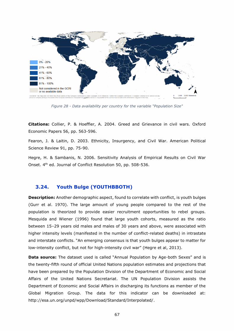
67
Figure 28 - Data availability per country for the variable “Population Size"
Citations: Collier, P. & Hoeffler, A. 2004. Greed and Grievance in civil wars. Oxford
Economic Papers 56, pp. 563-596.
Fearon, J. & Laitin, D. 2003. Ethnicity, Insurgency, and Civil War. American Political
Science Review 91, pp. 75-90.
Hegre, H. & Sambanis, N. 2006. Sensitivity Analysis of Empirical Results on Civil War
Onset. 4th ed. Journal of Conflict Resolution 50, pp. 508-536.
3.24. Youth Bulge (YOUTHBBOTH)
Description: Another demographic aspect, found to correlate with conflict, is youth bulges
(Gurr et al. 1970). The large amount of young people compared to the rest of the
population is theorized to provide easier recruitment opportunities to rebel groups.
Mesquida and Wiener (1996) found that large youth cohorts, measured as the ratio
between 15–29 years old males and males of 30 years and above, were associated with
higher intensity levels (manifested in the number of conflict-related deaths) in intrastate
and interstate conflicts. “An emerging consensus is that youth bulges appear to matter for
low-intensity conflict, but not for high-intensity civil war” (Hegre et al, 2013).
Data source: The dataset used is called “Annual Population by Age-both Sexes” and is
the twenty-fifth round of official United Nations population estimates and projections that
have been prepared by the Population Division of the Department of Economic and Social
Affairs of the United Nations Secretariat. The UN Population Division assists the
Department of Economic and Social Affairs in discharging its functions as member of the
Global Migration Group. The data for this indicator can be downloaded at:
http://esa.un.org/unpd/wpp/Download/Standard/Interpolated/.
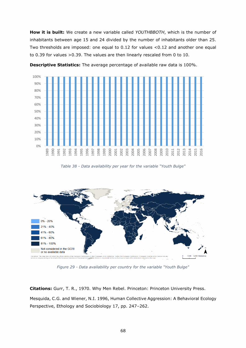
68
How it is built: We create a new variable called YOUTHBBOTH, which is the number of
inhabitants between age 15 and 24 divided by the number of inhabitants older than 25.
Two thresholds are imposed: one equal to 0.12 for values <0.12 and another one equal
to 0.39 for values >0.39. The values are then linearly rescaled from 0 to 10.
Descriptive Statistics: The average percentage of available raw data is 100%.
Table 38 - Data availability per year for the variable “Youth Bulge"
Figure 29 - Data availability per country for the variable “Youth Bulge"
Citations: Gurr, T. R., 1970. Why Men Rebel. Princeton: Princeton University Press.
Mesquida, C.G. and Wiener, N.I. 1996, Human Collective Aggression: A Behavioral Ecology
Perspective, Ethology and Sociobiology 17, pp. 247–262.
0%
10%
20%
30%
40%
50%
60%
70%
80%
90%
100%
19
89
19
90
19
91
19
92
19
93
19
94
19
95
19
96
19
97
19
98
19
99
20
00
20
01
20
02
20
03
20
04
20
05
20
06
20
07
20
08
20
09
20
10
20
11
20
12
20
13
20
14
20
15
20
16

69
Hegre, Håvard & Karlsen, Joakim & Nygård, Håvard & Strand, Håvard & Urdal, Henrik,
2013, Predicting Armed Conflict, 2010–2050. International Studies Quarterly. 57
Correlation between the variables and conflict intensity
Table 39 - Correlation matrix
Table 39 shows the correlation between all the variables. We observe that there seem to
be eleven cases where the variables are highly correlated, being the coefficient of
correlation8 (r) bigger than 0.7 (but still smaller than 0.9). Higher correlation is indicated
by a darker red colour. For instance, in the table above, we see that the coefficient of
correlation between the mortality rate index (MORT) and the GDP per capita index
(GDP_CAP) is 0.81.
8 r in statistics, the Pearson correlation coefficient is a measure of the linear correlation between
two variables X and Y. It has a value between +1 and −1, where 1 is total positive linear
correlation, 0 is no linear correlation, and −1 is total negative linear correlation.
(https://en.wikipedia.org/wiki/Pearson_correlation_coefficient)
CON_I
NT
CON_
NB
YRS_H
VC
CORR
UPT
DISPE
R
ECON
_ISO
EMPO
WER
ETHNI
C_SN
ETHNI
C_NPFOOD
FUEL_
EXP
GDP_
CAP
GOV_
EFF
HOMI
C
INEQ_
SWIIDMORT POP
REG_P
2
REG_
U
REPRE
SS
STRUC
T
UNEM
P
WATE
R
YOUT
HBBO
TH
CON_INT 1.00
CON_NB 0.25 1.00
YRS_HVC 0.67 0.16 1.00
CORRUPT 0.29 0.34 0.22 1.00
DISPER 0.32 0.37 0.20 0.25 1.00
ECON_ISO 0.11 0.11 0.10 0.24 -0.07 1.00
EMPOWER 0.20 0.32 0.12 0.39 0.16 0.09 1.00
ETHNIC_SN 0.24 0.09 0.16 0.11 0.21 0.03 0.16 1.00
ETHNIC_NP 0.16 0.12 0.18 0.19 0.04 0.07 0.03 0.12 1.00
FOOD 0.24 0.25 0.24 0.56 0.10 0.31 0.13 0.05 0.24 1.00
FUEL_EXP 0.05 0.07 0.06 0.08 0.03 -0.12 0.32 0.05 0.04 -0.23 1.00
GDP_CAP 0.25 0.32 0.20 0.61 0.14 0.31 0.10 0.09 0.26 0.78 -0.36 1.00
GOV_EFF 0.26 0.30 0.22 0.90 0.16 0.32 0.39 0.11 0.23 0.63 0.00 0.69 1.00
HOMIC 0.09 0.09 0.09 0.35 0.19 0.08 -0.23 -0.16 0.15 0.25 -0.11 0.26 0.33 1.00
INEQ_SWIID -0.05 -0.03 -0.06 0.10 -0.08 0.08 -0.12 -0.09 -0.05 0.19 -0.07 0.10 0.12 0.40 1.00
MORT 0.27 0.38 0.20 0.64 0.11 0.35 0.18 0.11 0.28 0.78 -0.13 0.81 0.69 0.33 0.23 1.00
POP 0.35 0.25 0.23 0.08 0.39 -0.07 0.16 0.04 0.00 -0.05 0.15 0.04 -0.05 -0.05 -0.12 -0.03 1.00
REG_P2 0.07 0.25 0.07 0.32 0.00 0.18 0.78 0.07 0.04 0.18 0.31 0.14 0.38 -0.22 -0.04 0.29 -0.07 1.00
REG_U 0.21 0.04 0.16 0.27 0.22 -0.02 -0.12 0.11 0.04 0.15 -0.20 0.22 0.24 0.22 0.05 0.14 0.00 -0.26 1.00
REPRESS 0.62 0.34 0.51 0.56 0.35 0.12 0.42 0.17 0.16 0.32 0.11 0.37 0.51 0.19 0.08 0.36 0.41 0.26 0.22 1.00
STRUCT 0.31 0.37 0.23 0.72 0.23 0.28 0.32 0.13 0.25 0.72 -0.12 0.77 0.77 0.30 0.15 0.78 0.05 0.31 0.22 0.48 1.00
UNEMP 0.02 0.02 0.06 0.08 0.05 -0.02 -0.04 0.03 -0.05 -0.09 0.06 -0.03 0.09 0.27 0.06 0.02 -0.14 -0.07 0.10 0.05 0.01 1.00
WATER 0.01 -0.04 0.02 0.02 -0.18 0.01 0.24 0.00 -0.07 -0.07 0.06 -0.11 0.01 -0.16 -0.05 -0.05 -0.06 0.23 -0.03 0.05 -0.05 0.16 1.00
YOUTHBBOTH 0.19 0.31 0.14 0.54 0.08 0.32 0.19 0.04 0.19 0.66 -0.14 0.67 0.59 0.32 0.30 0.82 -0.07 0.28 0.15 0.33 0.69 0.08 0.15 1.00
70
The correlation matrix is strictly symmetric (for instance, the correlation between MORT
and GDP_CAP is identical to the correlation between GDP_CAP and MORT), hence only the
lower-left part of the correlation matrix is shown here.
71
4. Composite Model
Based on economic, social, environmental and political data, the composite model gives
an insight into the contributing factors of conflict. It combines the 24 variables presented
in the previous chapter and provides a final score per country for each year. The present
chapter describes how the model works and what the outputs are.
4.1. Model description
The method used for combining the variables is a simple grouped mean method, its
calculation being much simpler and intuitively understood than other existing methods.
More specifically, the method reduces the number of variables in three steps: firstly from
24 (variables) to 10 (concepts); secondly from 10 (concepts) to 5 (risk areas), and from
5 (risk areas) to 1 (final score), using the arithmetic mean of the theoretically defined
groups (see Figure 30, p.72). One exception is applied for the concept “Social cohesion
and diversity”, in which the maximum value between the variables “Ethnic Power Change”
and “Ethnic Compilation” is firstly selected and then averaged with the two other variables
of this concept, namely “Corruption” and “Transnational ethnic bonds”.

72
Figure 30 - Influence of each variable in each concept on the overall score
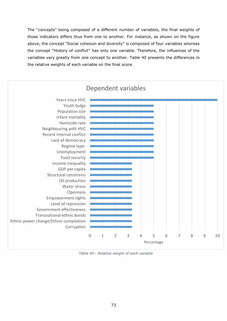
73
The “concepts” being composed of a different number of variables, the final weights of
those indicators differs thus from one to another. For instance, as shown on the figure
above, the concept “Social cohesion and diversity” is composed of four variables whereas
the concept “History of conflict” has only one variable. Therefore, the influences of the
variables vary greatly from one concept to another. Table 40 presents the differences in
the relative weights of each variable on the final score.
0 1 2 3 4 5 6 7 8 9 10
Corruption
Ethnic power change/Ethnic compilation
Transnational ethnic bonds
Government effectiveness
Level of repression
Empowerment rights
Openness
Water stress
Oil production
Structural constrains
GDP per capita
Income inequality
Food security
Unemployment
Regime type
Lack of democracy
Recent internal conflict
Neighbouring with HVC
Homicide rate
Infant mortality
Population size
Youth bulge
Years since HVC
Percentage
Dependent variables
Table 40 - Relative weight of each variable
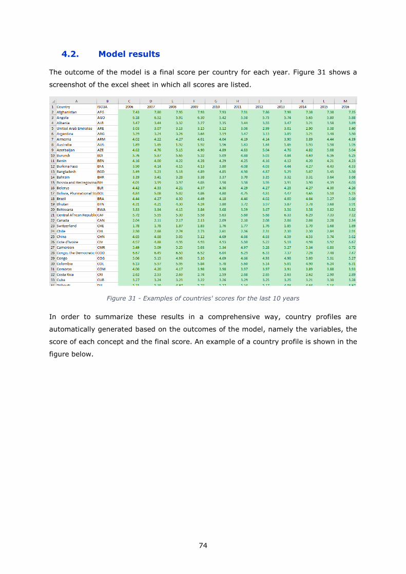
74
4.2. Model results
The outcome of the model is a final score per country for each year. Figure 31 shows a
screenshot of the excel sheet in which all scores are listed.
Figure 31 - Examples of countries' scores for the last 10 years
In order to summarize these results in a comprehensive way, country profiles are
automatically generated based on the outcomes of the model, namely the variables, the
score of each concept and the final score. An example of a country profile is shown in the
figure below.

75
Figure 32 – Example of a country profile

76
5. Conclusion
The latest version (2017) of the GCRI composite model has been greatly improved by
clearer documentation and improved traceability. The GCRI code has also been improved
with more transparency.
While there is still much room for improvement, the present data management provides
reliable data and the use of R scripts limits the possibility for human errors, while
development errors, if they happen, can easily be reported and effectively corrected.
The GCRI composite indicator is a tool that gives an easily interpretable presentation of
the variables. While it presents in a simple way how high the risk of conflict is at country
level, it also provides a great overview on the sector(s) that have the strongest
influence(s).
Further work should focus on improving specific aspects of the model. While the imputation
method used for the data is now (2017) uniform among the indicators, one improvement
could be to implement specialized methods for the variables depending on their nature.
There are also still some variables with very little data that rely on these imputations,
which introduces a considerable amount of noise. Having reliable data is crucial in
uncovering actual causal mechanisms and not random patterns in noisy data. Effort should
therefore also be put into finding improved data for the variables with the most serious
availability problems. This not only adds more input information, but also improves the
accuracy of imputed data.

77
6. References
Allansson, Marie, Erik Melander & Lotta Themnér (2017) Organized violence, 1989-2016.
Journal of Peace Research 54(4).
Bora, S., Ceccacci, I., Delgado, C., & Townsend. R. 2010. Food security and Conflict, World
Bank: World Development Report 2011.
Bueno de Mesquita, B., 1983. The War Trap. Yale: Yale University Press.
Buhaug, H. & Gleditsch, K.-S., 2008. Contagion or Confusion? Why Conflicts Cluster in
Space. 2nd ed. International Studies Quarterly 52, pp. 215-233.
Collier, P. et al., 2003. Breaking the Conflict Trap. Civil War and Development Policy. A
World Bank Policy Research Report. Oxford: Oxford University Press.
Collier, P. & Hoeffler, A. 2004. Greed and Grievance in civil wars. Oxford Economic Papers
56, pp. 563-596.
Dahl, Robert A. 1998. On Democracy. New Haven: Yale UP, pp. 36-38)
Danneman, N. & Hencken Ritter, E., 2014. Contagious Rebellion and Preemptive
Repression. Journal of Conflict Resolution 58 (2), pp. 254-279.
Dixon, J. 2009. What causes civil wars? Integrating Quantitative Research Findings.
International Studies Review 11, pp. 707-735.
Eck, Kristine and Lisa Hultman, 2007. ‘One-sided violence against civilians in war: insights
from new fatality data´, Journal of Peace Research 44(2): 233-246.
Esty, D. C. et al., 1998. State failure task force report: Phase II findings, Washington D.C.:
Central Intelligence Agency Directorate of Intelligence.
FAO, UN. 1996. Rome Declaration on Food Security and World Food Summit Plan of Action .
FAO, UN. 2003. Trade Reforms and Food Security: Conceptualizing the Linkages.
Fearon, J. & Laitin, D. 2003. Ethnicity, Insurgency, and Civil War. American Political
Science Review 91, pp. 75-90.
Fox, J. 2004. The rise of religious nationalism and conflict: Ethnic conflict and revolutionary
wars, 1945-2001. 6th ed. Journal of Peace Research 41, pp. 715-731.
Gartzke, E. 2007. The Capitalist Peace, American Journal of Political Science, Vol. 51, No.
1, pp. 166–19.
78
Gassert, F., Reig, P., Luo, T., & Maddocks, A. 2013. Aqueduct country and river basin
rankings: a weighted aggregation of spatially distinct hydrological indicators. Working
paper. Washington, DC: World Resources Institute.
Gleditsch, K. S., 2007. Transnational Dimensions of Civil War. Journal of Peace Research
44 (3), pp. 293-309.
Goldstone, J. A. et al. 2010. A Global Model for Forecasting Political Instability. American
Journal of Political Science 54, pp. 190-208.
Gurr, T. R., 1970. Why Men Rebel. Princeton: Princeton University Press.
Hegre, H. & Sambanis, N. 2006. Sensitivity Analysis of Empirical Results on Civil War
Onset. 4th ed. Journal of Conflict Resolution 50, pp. 508-536.
Hegre, Håvard & Karlsen, Joakim & Nygård, Håvard & Strand, Håvard & Urdal, Henrik,
2013, Predicting Armed Conflict, 2010–2050. International Studies Quarterly. 57
https://blog.bti-project.org/2014/02/19/conflict-management-is-at-a-low-point/
IEP, 2015, Global Peace Index: measuring peace, its causes and its economic value.
Kaufmann. D, Aart, K. & Mastruzzi, M. 2010. The Worldwide Governance Indicators:
Methodology and Analytical Issues. World Bank Policy Research Working Paper No. 5430
Martin, P., Thoenig, M., & Mayer, T. 2008. Civil Wars and International Trade, Journal of
the European Economic Association, pp.541–550.
Merkel, W. e. a. 2003. Defekte Demokratie Bd. 1: Theorie. Wiesbaden: VS Verlag für
Sozialwissenschaften
Mesquida, C.G. and Wiener, N.I. 1996, Human Collective Aggression: A Behavioral Ecology
Perspective, Ethology and Sociobiology 17, pp. 247–262.
Nome, M.-A., 2005. Transnational Ethnic Dimensions of Third-Party Interverntions in Civil
Conflicts, Oslo: University of Oslo.
O’Donnell, M. (2014). Corruption: A Rule of Law Agenda?. In: A. Hurwitz e. a., Civil war
and the rule of law : security, development, human rights, Lynne Rienner Publishers, p.
225.
Patel, P. 2013. Food sovereignty is next big idea. Financial Times.
Poe, Steven P. Carey, Sabine C. & Vazquez, Tanya C. 2001. How are these pictures
Different? A quantitative comparison of the US State Department and Amnesty
International human rights reports, 1976-1995. Human Rights Quarterly 23.3, pp. 650-
677.

79
Regan, P. M. & Norton, D. 2005. Greed, Grievance and Mobilization in Civil Wars. 3rd ed.
Journal of Conflict Resolution 49, pp. 319-336.
Reynal-Querol, M.. 2002. Ethnicity, Political Systems, and Civil Wars, Sage Publications:
Journal of Conflict Resolution, Vol. 46, pp. 29-54.
Sambanis, N., 2001. Do ethnic and non-ethnic civil wars have the same cause? A
theoretical and empirical inquiry (Part I). Journal of Conflict Resolution 45 (3), pp. 259-
282.
Solt, Frederick. 2016. The Standardized World Income Inequality Database. Social Science
Quarterly 97. SWIID Version 5.1.
Sundberg, Ralph, Kristine Eck and Joakim Kreutz, 2012, "Introducing the UCDP NonState
Conflict Dataset", Journal of Peace Research, March 2012, 49:351-362
Vogt, M., Bormann, N.-C., Rüegger, S., Cederman, L.-E., Hunziker, P., & Girardin, L. 2015.
Integrating Data on Ethnicity, Geography, and Conflict: The Ethnic Power Relations
Dataset Family. 7th ed. Journal of Conflict Resolution 59, 1327-1342.
Vreeland, J. 2008. The Effect of Political Regime on Civil War: Unpacking Anocracy. 3rd ed.
Journal of Conflict Resolution 52, pp. 401-425.
Wimmer, A., Cederman, L.-E. & Min, B., 2009. Ethnic Polictics and Armed Conflict: A
Configurational Analysis of a New Global Data Set. American Sociological Review, pp. 316-
337.
7. List of figures
Figure 1 - Data availability per country for the variable “Regime Type” ...................... 14
Figure 2 - Data availability per country for the variable “Lack of Democracy" .............. 16
Figure 3 - Data availability per country for the variable “Government Effectiveness” .... 18
Figure 4 - Data availability per country for the variable “Level of Repression” ............. 19
Figure 5 - Data availability per country for the variable “Empowerment Rights” .......... 21
Figure 6 - Data availability per country for the variable “Recent Internal Conflict” ....... 24
Figure 7 - Data availability per country for the variable “Neighbouring Conflict” .......... 27
Figure 8 - Data availability per country for the variable “Years Since Highly Violent Conflict”
......................................................................................................................... 30
Figure 9 - Data availability per country for the variable “Corruption” .......................... 32

80
Figure 10 - Data availability per country for the variable “Ethnic Power Change” ......... 37
Figure 11 - Data availability per country for the variable “Ethnic Compilation" ............. 39
Figure 12 - Data availability per country for the variable “Transnational Ethnic Bonds” . 42
Figure 13 - Data availability per country for the variable “Homicide Rate” .................. 44
Figure 14 - Data availability per country for the variable “Infant Mortality" ................. 45
Figure 15 - Data availability per country for the variable “GDP per capita" .................. 47
Figure 16 - Data availability per country for the variable “Income Inequality" ............. 49
Figure 17 - Data availability per country for the variable “Foreign" ............................ 51
Figure 18 - Data availability per country for the variable “Foreign2"........................... 52
Figure 19 - Data availability per country for the variable “Export" .............................. 53
Figure 20 - Data availability per country for the variable “Diet" ................................. 55
Figure 21 - Data availability per country for the variable “Price Level" ........................ 56
Figure 22 - Data availability per country for the variable “Nourishment" ..................... 57
Figure 23 - Data availability per country for the variable “Volatility"........................... 58
Figure 24 - Data availability per country for the variable “Unemployment" ................. 60
Figure 25 - Data availability per country for the variable “Water Stress" ..................... 62
Figure 26 - Data availability per country for the variable “Oil Producer" ...................... 63
Figure 27 - Data availability per country for the variable “Structural Constrains" ......... 65
Figure 28 - Data availability per country for the variable “Population Size" ................. 67
Figure 29 - Data availability per country for the variable “Youth Bulge" ...................... 68
Figure 30 - Influence of each variable in each concept on the overall score................. 72
Figure 31 - Examples of countries' scores for the last 10 years ................................. 74
Figure 32 – Example of a country profile ................................................................ 75
8. List of tables
Table 1 - The index’s structure ................................................................................ 4
Table 2 - Variable sources (first part) ...................................................................... 5
Table 3 - Variable sources (second part) .................................................................. 8

81
Table 4 - Descriptive statistics .............................................................................. 10
Table 5 - Regime type coding rules from Goldstone et al. based on Policy IV scales (2010)
......................................................................................................................... 12
Table 6 - Regime type scores ................................................................................ 13
Table 7 - Data availability per year for the variable “Regime Type” ............................ 14
Table 8 - Data availability per year for the variable “Lack of Democracy" ................... 16
Table 9 - Data availability per year for the variable “Government Effectiveness” ......... 17
Table 10 - Data availability per year for the variable “Level of Repression” ................. 19
Table 11 - Data availability per year for the variable “Empowerment Rights” .............. 21
Table 12 - Subnational Intensity ........................................................................... 23
Table 13 - National Intensity ................................................................................ 24
Table 14 - Data availability per year for the variable “Recent Internal Conflict” ........... 24
Table 15 - Data availability per year for the variable “Neighbouring Conflict” .............. 27
Table 16 - Data availability per year for the variable “Years Since Highly Violent Conflict “
......................................................................................................................... 29
Table 17 - Data availability per year for the variable “Corruption” ............................. 31
Table 18 - Data availability per year for the variable “Ethnic Power Change” ............... 37
Table 19 - Ethnic compilation score ....................................................................... 38
Table 20 - Data availability per year for the variable “Ethnic Compilation" .................. 39
Table 21 - Data availability per year for the variable “Transnational Ethnic Bonds” ...... 41
Table 22 - Data availability per year for the variable “Homicide Rate” ........................ 43
Table 23 - Data availability per year for the variable “Infant Mortality" ....................... 45
Table 24 - Data availability per year for the variable “GDP per capita" ....................... 46
Table 25 - Data availability per year for the variable “Income Inequality" ................... 48
Table 26 - Data availability per year for the variable “Foreign" .................................. 50
Table 27 - Data availability per year for the variable “Foreign2" ................................ 51
Table 28 - Data availability per year for the variable “Export" ................................... 52
Table 29 - Data availability per year for the variable “Diet" ....................................... 55
Table 30 - Data availability per year for the variable “Price Level" ............................. 56
82
Table 31 - Data availability per year for the variable “Nourishment" .......................... 57
Table 32 - Data availability per year for the variable “Volatility" ................................ 58
Table 33 - Data availability per year for the variable “Unemployment" ....................... 60
Table 34 - Data availability per year for the variable “Water Stress" .......................... 61
Table 35 - Data availability per year for the variable “Oil Producer" ........................... 63
Table 36 - Data availability per year for the variable “Structural Constrains" ............... 65
Table 37 - Data availability per year for the variable “Population Size" ....................... 66
Table 38 - Data availability per year for the variable “Youth Bulge" ........................... 68
Table 39 - Correlation matrix ................................................................................ 69
Table 40 - Relative weight of each variable ............................................................. 73

83
1
How to obtain EU publications
Our publications are available from EU Bookshop (http://bookshop.europa.eu),
where you can place an order with the sales agent of your choice.
The Publications Office has a worldwide network of sales agents.
You can obtain their contact details by sending a fax to (352) 29 29-42758.
Europe Direct is a service to help you find answers to your questions about the European Union
Free phone number (*): 00 800 6 7 8 9 10 11
(*) Certain mobile telephone operators do not allow access to 00 800 numbers or these calls may be billed.
A great deal of additional information on the European Union is available on the Internet.
It can be accessed through the Europa server http://europa.eu
2
JRC Mission
As the Commission’s
in-house science service,
the Joint Research Centre’s
mission is to provide EU
policies with independent,
evidence-based scientific
and technical support
throughout the whole
policy cycle.
Working in close
cooperation with policy
Directorates-General,
the JRC addresses key
societal challenges while
stimulating innovation
through developing
new methods, tools
and standards, and sharing
its know-how with
the Member States,
the scientific community
and international partners.
Serving society Stimulating innovation Supporting legislation
doi:10.2760/44005
ISBN 978-92-79-75768-6
doi: 10.2788/705817
KJ-N
A-2
8860-E
N-N