conditioning probabilistic databases dan olteanu (oxford ... · example: probabilistic database...

Conditioning Probabilistic DatabasesDan Olteanu (Oxford University Computing Laboratory)

Joint work with Christoph Koch (Cornell University Database Systems Group)

Main goals of the MayBMS project

Create a scalable DBMS for uncertain/probabilistic data

1 Representation and storage mechanisms

2 Uncertainty-aware query and data manipulation language

3 Efficient processing techniques for queries and constraints

This talk covers aspects of (3).

MayBMS available at sourceforge.net !

Conditioning c-table-like Probabilistic Databases

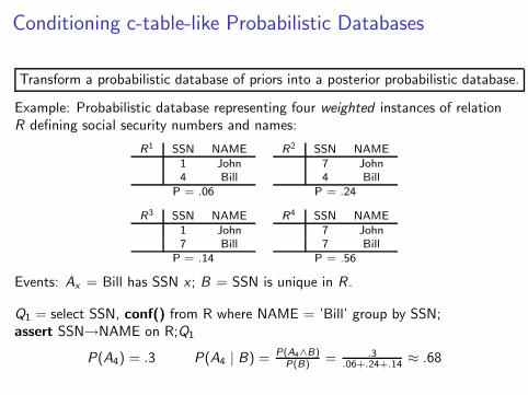
Transform a probabilistic database of priors into a posterior probabilistic database.

Example: Probabilistic database representing four weighted instances of relationR defining social security numbers and names:

R1 SSN NAME1 John4 Bill


P = .06 P = .24



P = .14 P = .56

Events: Ax = Bill has SSN x ; B = SSN is unique in R .

Q1 = select SSN, conf() from R where NAME = ’Bill’ group by SSN;assert SSN→NAME on R;Q1

P(A4) = .3 P(A4 | B) = P(A4∧B)P(B) = .3

.06+.24+.14 ≈ .68

Challenges

Conditioning/confidence computation is NP-hard on succinct representations.

No prior work on conditioning probabilistic databases (i.e., on using assert)

Some prior work on confidence computation (MystiQ, Trio, MayBMS, . . .)

Exact versus approximate computation.

Approximation problematic for compositional query languages forprobabilistic databases.

◮ Introduced errors aggregate and grow.◮ conf() used in comparison predicates.

Materialize the (succinct) probabilistic database result of conditioning.

assert is natural for data cleaning under possible worlds semantics.

Our representation system: U-Relational Databases

Discrete independent (random) variables.

Representation: U-relations + table W representing distributions.

The schema of each U-relation consists of◮ a set of column pairs WSD = (Var → Dom) representing variable assignments,◮ a set of value columns,◮ (a tuple id column).

W Var Dom Pj 1 .2j 7 .8b 4 .3b 7 .7

UR WSD SSN NAME{j 7→ 1} 1 John{j 7→ 7} 7 John{b 7→ 4} 4 Bill{b 7→ 7} 7 Bill

Properties of U-relational databases

Complete representation system for finite sets of possible worlds.

Purely relational representation of uncertainty at attribute-level.

Efficient relational evaluation of SPJ queries (without conf()).


W Var Dom Pj 1 .2j 7 .8b 4 .3b 7 .7



W Var Dom Pj 1 .2j 7 .8b 4 .3b 7 .7




P = .2 · .3 = .06 P = .8 · .3 = .24



P = .2 · .7 = .14 P = .8 · .7 = .56

Queries on U-Relational Databases

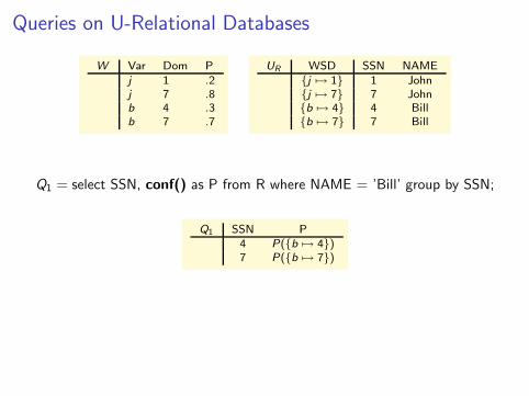
W Var Dom Pj 1 .2j 7 .8b 4 .3b 7 .7


Q1 = select SSN, conf() as P from R where NAME = ’Bill’ group by SSN;

Q1 SSN P4 P({b 7→ 4})7 P({b 7→ 7})

What makes confidence computation hard?1 Succinct representation of uncertainty.

◮ Each tuple in a probabilistic database is associated with a world-set descriptor

that succinctly encodes the set of worlds containing that tuple.World-set descriptor = Conjunction of variable assignments.Examples: {j → 1}, {j → 1, b → 4}.

◮ Arbitrary combinations of input world-set descriptors produced by query joins.

2 Queries with projections can create duplicate answer tuples.◮ Distinct tuples can be associated with sets of world-set descriptors.

Set of world-set descriptors = DNF expression over variable assigments.Examples: {{j → 1}} and {{j → 1}, {j → 1, b → 4}, {b → 7}}.

3 #SAT (Model counting) is #P-hard for arbitrary DNF expressions.◮ Model counting is a special case of confidence computation.◮ Arbitrary sets of world-set descriptors can be created by queries.◮ The sets of models of different conjunctions in a DNF expression can overlap

and have exponential size.

Knowledge Compilation Techniques to the Rescue

Useful for compiling formulas into propositional theories with tractableproperties, e.g., (#)SAT.ROBDDs (Bryant), d-NNFs (Darwiche), and variations thereof.

Successfully applied to system modelling and verification.

In this paper: ws-sets compiled into ws-trees.

more succinct than OBDDs and similar to d-NNFs

structurally limited (trees) and with multistate variables

ws-sets can be compiled into ws-trees of exponential sizebut like OBDDs tend to behave well in practice

Idea behind ws-tree construction: Given a tuple t with a ws-set S , partition S

into independent subsets (exploit contextual independence)

by variable elimination (Davis-Putnam procedure)

Building ws-trees

S = {{x 7→ 1}, {x 7→ 2, y 7→ 1}, {x 7→ 2, z 7→ 1}, {u 7→ 1, v 7→ 1}, {u 7→ 2}}

Assume domx = {1, 2, 3} and domy = domz = domu = domv = {1, 2}.

⊗

⊕

∅

x 7→ 1

⊗

x 7→ 2

⊕

∅

y 7→ 1

⊕

∅

z 7→ 1

⊕

⊕

u 7→ 1

∅

v 7→ 1

∅

u 7→ 2

Apply independence partitioning to S :

left: {{x 7→ 1}, {x 7→ 2, y 7→ 1}, {x 7→ 2, z 7→ 1}}

right: {{u 7→ 1, v 7→ 1}, {u 7→ 2}}.

Building ws-trees

S = {{x 7→ 1}, {x 7→ 2, y 7→ 1}, {x 7→ 2, z 7→ 1}, {u 7→ 1, v 7→ 1}, {u 7→ 2}}


⊗

⊕

∅

x 7→ 1

⊗

x 7→ 2

⊕

∅

y 7→ 1

⊕

∅

z 7→ 1

⊕

⊕

u 7→ 1

∅

v 7→ 1

∅

u 7→ 2

Apply variable elimination to {{x 7→ 1}, {x 7→ 2, y 7→ 1}, {x 7→ 2, z 7→ 1}}.

left: x 7→ 1 : ∅

right: x 7→ 2 : {{y 7→ 1}, {z 7→ 1}}.

Building ws-trees

S = {{x 7→ 1}, {x 7→ 2, y 7→ 1}, {x 7→ 2, z 7→ 1}, {u 7→ 1, v 7→ 1}, {u 7→ 2}}


⊗

⊕

∅

x 7→ 1

⊗

x 7→ 2

⊕

∅

y 7→ 1

⊕

∅

z 7→ 1

⊕

⊕

u 7→ 1

∅

v 7→ 1

∅

u 7→ 2

Apply independence partitioning to {{y 7→ 1}, {z 7→ 1}}.

left: {{y 7→ 1}}

right: {{z 7→ 1}}

Building ws-trees

S = {{x 7→ 1}, {x 7→ 2, y 7→ 1}, {x 7→ 2, z 7→ 1}, {u 7→ 1, v 7→ 1}, {u 7→ 2}}


⊗

⊕

∅

x 7→ 1

⊗

x 7→ 2

⊕

∅

y 7→ 1

⊕

∅

z 7→ 1

⊕

⊕

u 7→ 1

∅

v 7→ 1

∅

u 7→ 2

Apply variable elimination to {{u 7→ 1, v 7→ 1}, {u 7→ 2}}.

left: u 7→ 1 : {{v 7→ 1}}

right: u 7→ 2 : ∅

Confidence computation using ws-trees

S = {{x 7→ 1}, {x 7→ 2, y 7→ 1}, {x 7→ 2, z 7→ 1}, {u 7→ 1, v 7→ 1}, {u 7→ 2}}

Assume: domx = {1, 2, 3} and domy = domz = domu = domv = {1, 2}.

x.17→ 1, x

.47→ 2, y

.27→ 1, z

.47→ 1, u

.77→ 1, u

.37→ 2, v

.57→ 1.

⊗ 0.7578

⊕ 0.308

∅ 1.0

x.17→ 1

⊗ 0.52

x.47→ 2

⊕ 0.2

∅ 1.0

y.27→ 1

⊕ 0.4

∅ 1.0

z.47→ 1

⊕ 0.65

⊕ 0.5

u.77→ 1

∅ 1.0

v.57→ 1

∅ 1.0

u.37→ 2

P(S) = 0.7578.

Conditioning using ws-trees

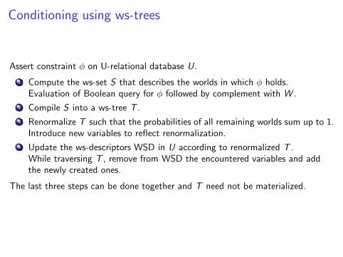
Assert constraint φ on U-relational database U.

1 Compute the ws-set S that describes the worlds in which φ holds.Evaluation of Boolean query for φ followed by complement with W .

2 Compile S into a ws-tree T .

3 Renormalize T such that the probabilities of all remaining worlds sum up to 1.Introduce new variables to reflect renormalization.

4 Update the ws-descriptors WSD in U according to renormalized T .While traversing T , remove from WSD the encountered variables and addthe newly created ones.

The last three steps can be done together and T need not be materialized.

Data cleaning example: Evaluate

W Var Dom Pj 1 .2j 7 .8b 4 .3b 7 .7


Keep only those worlds that satisfy the key constraint on R :

assert SSN→ NAME on R;

Expressed as a Boolean query as a complement of π∅(R ⊲⊳φ R) whereφ := (1.SSN = 2.SSN ∧ 1.NAME 6= 2.NAME ). On U-relation UR ,

πWSD(UR ⊲⊳φ∧1.WSD consistent with 2.WSD UR).

Result consists of WSD {j 7→ 7, b 7→ 7}. Its complement with the (entire)world-set given by W is:

{{j 7→ 1}, {j 7→ 7, b 7→ 4}}, or (equivalently)

{{b 7→ 4}, {b 7→ 7, j 7→ 1}}.

Data cleaning example: Compile and Renormalize

W Var Dom Pj 1 .2j 7 .8b 4 .3b 7 .7


SSN→NAME holds in the worlds defined by S = {{j 7→ 1}, {j 7→ 7, b 7→ 4}}.Compile S into a ws-tree and renormalize the latter.

⊕

∅

j.27→ 1

⊕

j.87→ 7

∅

b.37→ 4

⊕

∅

j ′.2.447→ 1

⊕

j ′.8·.3.447→ 7

∅

b′17→ 4

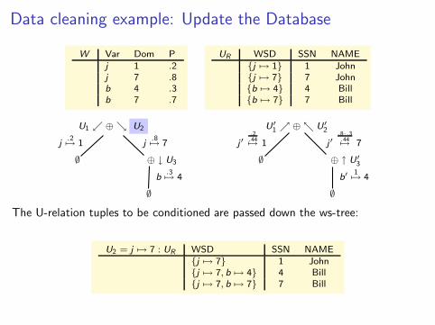
Data cleaning example: Update the Database

W Var Dom Pj 1 .2j 7 .8b 4 .3b 7 .7


U1 ւ ⊕ ց U2

∅

j.27→ 1

⊕ ↓ U3

j.87→ 7

∅

b.37→ 4

U′

1 ր ⊕ տ U′

2

∅

j ′.2.447→ 1

⊕ ↑ U′

3

j ′.8·.3.447→ 7

∅

b′17→ 4

The U-relation tuples to be conditioned are passed down the ws-tree:

U1 = j 7→ 1 : UR WSD SSN NAME{j 7→ 1} 1 John{j 7→ 1, b 7→ 4} 4 Bill{j 7→ 1, b 7→ 7} 7 Bill


W Var Dom Pj 1 .2j 7 .8b 4 .3b 7 .7


U1 ւ ⊕ ց U2

∅

j.27→ 1

⊕ ↓ U3

j.87→ 7

∅

b.37→ 4

U′

1 ր ⊕ տ U′

2

∅

j ′.2.447→ 1

⊕ ↑ U′

3

j ′.8·.3.447→ 7

∅

b′17→ 4


U2 = j 7→ 7 : UR WSD SSN NAME{j 7→ 7} 1 John{j 7→ 7, b 7→ 4} 4 Bill{j 7→ 7, b 7→ 7} 7 Bill


W Var Dom Pj 1 .2j 7 .8b 4 .3b 7 .7


U1 ւ ⊕ ց U2

∅

j.27→ 1

⊕ ↓ U3

j.87→ 7

∅

b.37→ 4

U′

1 ր ⊕ տ U′

2

∅

j ′.2.447→ 1

⊕ ↑ U′

3

j ′.8·.3.447→ 7

∅

b′17→ 4


U3 = b 7→ 4 : U2 WSD SSN NAME{j 7→ 7, b → 4} 1 John{j 7→ 7, b 7→ 4} 4 Bill


W Var Dom Pj 1 .2j 7 .8b 4 .3b 7 .7


U1 ւ ⊕ ց U2

∅

j.27→ 1

⊕ ↓ U3

j.87→ 7

∅

b.37→ 4

U′

1 ր ⊕ տ U′

2

∅

j ′.2.447→ 1

⊕ ↑ U′

3

j ′.8·.3.447→ 7

∅

b′17→ 4

Replace old variables by new variables in the U-relations to be pushed up thenormalized ws-tree:

U′

3 = Replace b by b′ in U3 WSD SSN NAME{j 7→ 7, b′ 7→ 4} 1 John{j 7→ 7, b′ 7→ 4} 4 Bill


W Var Dom Pj 1 .2j 7 .8b 4 .3b 7 .7


U1 ւ ⊕ ց U2

∅

j.27→ 1

⊕ ↓ U3

j.87→ 7

∅

b.37→ 4

U′

1 ր ⊕ տ U′

2

∅

j ′.2.447→ 1

⊕ ↑ U′

3

j ′.8·.3.447→ 7

∅

b′17→ 4

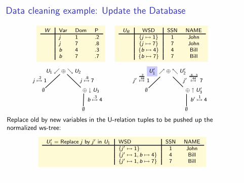
Replace old by new variables in the U-relation tuples to be pushed up thenormalized ws-tree:

U′

2 = Replace j by j ′ in U′

3 WSD SSN NAME{j ′ 7→ 7, b′ 7→ 4} 1 John{j ′ 7→ 7, b′ 7→ 4} 4 Bill


W Var Dom Pj 1 .2j 7 .8b 4 .3b 7 .7


U1 ւ ⊕ ց U2

∅

j.27→ 1

⊕ ↓ U3

j.87→ 7

∅

b.37→ 4

U′

1 ր ⊕ տ U′

2

∅

j ′.2.447→ 1

⊕ ↑ U′

3

j ′.8·.3.447→ 7

∅

b′17→ 4

Replace old by new variables in the U-relation tuples to be pushed up thenormalized ws-tree:

U′

1 = Replace j by j ′ in U1 WSD SSN NAME{j ′ 7→ 1} 1 John{j ′ 7→ 1, b 7→ 4} 4 Bill{j ′ 7→ 1, b 7→ 7} 7 Bill


W Var Dom Pj 1 .2j 7 .8b 4 .3b 7 .7


U1 ւ ⊕ ց U2

∅

j.27→ 1

⊕ ↓ U3

j.87→ 7

∅

b.37→ 4

U′

1 ր ⊕ տ U′

2

∅

j ′.2.447→ 1

⊕ ↑ U′

3

j ′.8·.3.447→ 7

∅

b′17→ 4

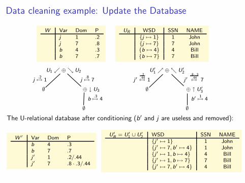
The U-relational database after conditioning (b′ and j are useless and removed):

W ′ Var Dom Pb 4 .3b 7 .7j ′ 1 .2/.44j ′ 7 .8 · .3/.44

U′

R= U′

1 ∪ U′

2 WSD SSN NAME{j ′ 7→ 1} 1 John{j ′ 7→ 7, b′ 7→ 4} 1 John{j ′ 7→ 1, b 7→ 4} 4 Bill{j ′ 7→ 1, b 7→ 7} 7 Bill{j ′ 7→ 7, b′ 7→ 4} 4 Bill

Experiments

Tuple-independent TPC-H DataQueries

1 select distinct true from customer c, orders o, lineitem l where c.mktsegment =

’BUILDING’ and c.custkey = o.custkey and o.orderkey = l.orderkey and o.orderdate >

’1995-03-15’

2 select distinct true from lineitem where shipdate between ’1994-01-01’ and ’1996-01-01’

and discount between ’0.05’ and ’0.08’ and quantity < 24

Query Size of TPC-H #Input Size of Userws-desc. Scale Vars ws-set Time(s)

0.01 77215 9836 5.10Q1 3 0.05 382314 43498 99.76

0.10 765572 63886 356.560.01 60175 3029 0.20

Q2 1 0.05 299814 15545 8.240.10 600572 30948 33.68

Tractable cases of query evaluation on probabilistic databases beyond safe plans:

Using OBDDs for Efficient Query Evaluation on Probabilistic Databases.O. and Huang. In Proc. SUM 2008.

Lazy versus Eager Query Plans for Tuple-Independent Probabilistic Databases.O., Huang, and Koch. 2008.

#P-hard casesInput: ws-sets similar to those associated with the answers of non-safe Booleanqueries on probabilistic databases.

Compared agorithms for confidence computation

INDVE: independence partitioning and variable elimination

VE: only variable elimination

KL: (adapted) optimal Monte Carlo simulation based on Karp-Luby FPRASfor DNF countingGiven a DNF formula with m clauses, compute an (ǫ, δ)-approximation c ofthe number of solutions c of the DNF formula such that

Pr[|c − c | ≤ ǫ · c] ≥ 1 − δ

for any given 0 < ǫ < 1, 0 < δ < 1. It does so within ⌈4 · m · log(2/δ)/ǫ2⌉iterations of an efficiently computable estimator.

INDVE is now part of the MayBMS engine!

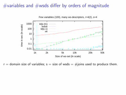
#variables and #wsds differ by orders of magnitude

0.01

0.1

1

10

100

1000

50k25k10k5k2k1k

time

in s

ec (

ln s

cale

)

Size of ws-set (ln scale)

Few variables (100), many ws-descriptors, r=4(2), s=4

kl(e.01)indve

kl(e.1)ve

r = domain size of variables; s = size of wsds = #joins used to produce them.

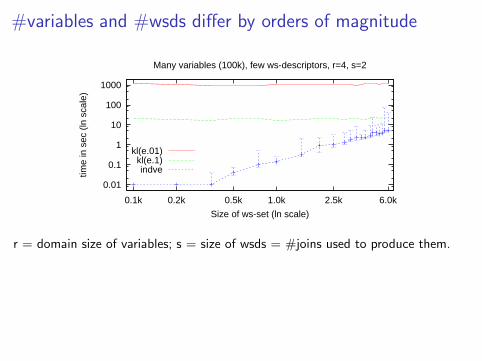
#variables and #wsds differ by orders of magnitude

0.01

0.1

1

10

100

1000

6.0k2.5k1.0k0.5k0.2k0.1k

time

in s

ec (

ln s

cale

)


Many variables (100k), few ws-descriptors, r=4, s=2

kl(e.01)kl(e.1)indve

r = domain size of variables; s = size of wsds = #joins used to produce them.

#variables and #wsds are close: Easy-hard-easy pattern

0.01

0.1

1

10

100

1000

10000

5000825500200905

time

in s

ec (

ln s

cale

)


Number of variables close to ws-set size, 70 variables, r=4, s=4

indve(ymax)indve(median)

kl(e.001)indve(ymin)

Known that the computation becomes harder in this case. The hard area issmaller for SAT than for #SAT.

Thanks!

Order of Variable Elimination Matters!

S = {{x 7→ 1}, {x 7→ 2, y 7→ 1}, {x 7→ 2, z 7→ 1}, {u 7→ 1, v 7→ 1}, {u 7→ 2}}


⊕

⊕y 7→ 1

⊗u 7→ 1

⊕

∅v 7→ 1

⊕

⊕(α)z 7→ 2

∅x 7→ 1

∅x 7→ 2

α

∅u 7→ 2

⊕y 7→ 2

∅x 7→ 1

⊗x 7→ 2

⊕

∅z 7→ 1

⊕(β)

∅u 7→ 2

⊕u 7→ 1

∅v 7→ 1

βx 7→ 3

Different ws-tree for the same ws-set S!

conditioning probabilistic databases dan olteanu (oxford ... · example: probabilistic database...

Documents