sensors

Article

Condition Assessment of Foundation Piles and UtilityPoles Based on Guided Wave Propagation Usinga Network of Tactile Transducers and SupportVector Machines

Ulrike Dackermann 1 ID , Yang Yu 2,*, Ernst Niederleithinger 3, Jianchun Li 2

and Herbert Wiggenhauser 3

1 Centre for Infrastructure Engineering and Safety, School of Civil and Environmental Engineering,Faculty of Engineering, University of New South Wales (UNSW), Sydney, NSW 2052, Australia;u.dackermann@unsw.edu.au

2 Centre for Built Infrastructure Research, School of Civil and Environmental Engineering,Faculty of Engineering and Information Technology, University of Technology, Sydney, NSW 2007, Australia;jianchun.li@uts.edu.au

3 Division 8.2, German Federal Institute for Material Research and Testing (BAM), 12205 Berlin, Germany;ernst.niederleithinger@bam.de (E.N.); herbert.wiggenhauser@bam.de (H.W.)

* Correspondence: yang.yu@uts.edu.au; Tel.: +61-2-9514-9059

Received: 15 November 2017; Accepted: 15 December 2017; Published: 18 December 2017

Abstract: This paper presents a novel non-destructive testing and health monitoring system usinga network of tactile transducers and accelerometers for the condition assessment and damageclassification of foundation piles and utility poles. While in traditional pile integrity testing an impacthammer with broadband frequency excitation is typically used, the proposed testing system utilizesan innovative excitation system based on a network of tactile transducers to induce controllednarrow-band frequency stress waves. Thereby, the simultaneous excitation of multiple stress wavetypes and modes is avoided (or at least reduced), and targeted wave forms can be generated. The newtesting system enables the testing and monitoring of foundation piles and utility poles where the topis inaccessible, making the new testing system suitable, for example, for the condition assessment ofpile structures with obstructed heads and of poles with live wires. For system validation, the newsystem was experimentally tested on nine timber and concrete poles that were inflicted with severaltypes of damage. The tactile transducers were excited with continuous sine wave signals of 1 kHzfrequency. Support vector machines were employed together with advanced signal processingalgorithms to distinguish recorded stress wave signals from pole structures with different typesof damage. The results show that using fast Fourier transform signals, combined with principalcomponent analysis as the input feature vector for support vector machine (SVM) classifiers withdifferent kernel functions, can achieve damage classification with accuracies of 92.5% ± 7.5%.

Keywords: Structural Health Monitoring; non-destructive testing; sensor network; tactile transducers;guided waves; support vector machine; principal component analysis; foundation piles; utilitypoles; pipelines

1. Introduction

Structural Health Monitoring (SHM) is a wide and multi-disciplinary field dealing with innovativemethods for monitoring structural safety, integrity and performance without affecting the operation ofthe structure [1]. For civil engineering structures, non-destructive testing (NDT) combined with activeSHM presents the future in infrastructure management including condition assessment, monitoring

Sensors 2017, 17, 2938; doi:10.3390/s17122938 www.mdpi.com/journal/sensors

Sensors 2017, 17, 2938 2 of 16

and maintenance. For foundation piles and utility poles, inspection routines are still primarily basedon traditional methods, including visual inspection, sounding and resistance drilling. While visualinspection is undoubtedly one of the oldest assessment methods, it is limited to accessible areasand surface damage, and like sounding and resistance drilling, its reliability and accuracy is highlydependent on the experience of the operator [2]. As an alternative to these limited low-tech conditionassessment methods, guided wave-based methods, such as pile integrity testing, are established testingmethods for concrete piles and deep foundations that provide objective quantitative data, and areable to potentially detect internal damage and evaluate the health condition of non-accessible areassuch as embedded sections of foundation piles and utility poles [3–5]. In guided wave testing, stresswaves are generated in a structure, typically through a sudden pressure or deformation caused byan impact excitation, which subsequently propagate through the structure similar to the propagationof sound waves through air [6]. In pile and pole structures, the wave types generated through guidedwave testing are longitudinal, bending and Rayleigh waves. While longitudinal and bending wavesare body waves that propagate inside the structure along hemispherical wave fronts, Rayleigh wavestravel away from the disturbance along the surface. Due to the dependency of the wave’s velocityto the modulus of elasticity, Poisson’s ratio, density and geometry of the structure, analyzing stresswaves can give indications of a structure’s soundness condition [7,8].

While stress-wave-based techniques have promising potentials in damage detection and healthmonitoring of foundation piles and utility poles, some important issues associated with the uncertaintyof wave propagation in in-service structures must be considered. These issues include the effect of soilembedment coupled with unknown soil and structure conditions below ground line; the generationof different wave modes due to broadband frequency excitation; the complexity of the structure’smaterial properties, which can be non-homogeneous (reinforced concrete) or anisotropic (timber),and can include inhomogeneities such as small voids, honey-comb or natural defects; the sensitivityto environmental changes such as moisture and temperature fluctuations; and the influence of theimpact location [9]. As such, in pile integrity testing, the excitation is typically applied at the top of thepile, which will generate pure longitudinal waves. For the testing of in-situ poles, however, which aretypically 10 m to 12 m long with a soil embedment of 1 m to 1.6 m, a top excitation is not feasible.Hence, a side impact must be performed, resulting in more complex wave propagation and responsewave patterns. Here, longitudinal waves, bending waves and Rayleigh waves will be generated atthe same time. Due to the broadband excitation from an impact hammer, various wave modes of thedifferent wave types will be generated simultaneously. Understanding the wave propagation behaviorin pile and pole structures is essential for the design of testing techniques and for the analysis of stresswave measurements for condition assessment and damage detection. Due to the vast complexity of thewave propagation, innovative testing and advanced signal processing techniques must be applied todeal with the issues described above. Using machine learning techniques for the condition assessmentand monitoring of foundation piles and utility poles has previously provided promising results forin-field integrity testing [3,10] and is further explored in this study.

This paper proposes a novel testing and analysis system that uses a network of low-cost tactiletransducer technology from the audio industry (instead of a broadband frequency excitation usingan impact hammer) to induce controlled narrow-band frequency stress wave signals, avoiding or atleast minimizing the generation of multiple wave types and modes. A network of accelerometers,arranged in three rings, is used to capture the wave propagation along the pile or pole structure.The innovative system is tested on a number of undamaged and damaged timber and concrete polesin the laboratory and in the field (with soil embedment), with controllable and axisymmetric excitation.For signal processing, fast Fourier transform (FFT) data combined with principal component analysis(PCA) are used to analyze the captured time-domain stress wave signals for features extraction.To evaluate the health condition and damage states of the poles, different types of classification modelsbased on state-of-the art machine learning techniques using support vector machines (SVMs) aretrained. The proposed method is based on the assumption that similar types of damage result in

Sensors 2017, 17, 2938 3 of 16

similar patterns in stress wave measurements, which can be extracted and identified using the methodpresented. The results of this study show that the proposed testing and analysis system has greatpotential to identify the damage condition of pile/pole structures.

2. New Wave Excitation System Based on Tactile Transducers

The proposed testing system utilizes low-cost tactile transducer technology from the audioindustry for the controlled induction of narrow-band frequency stress waves in foundation piles andutility poles. A tactile transducer is an electro-mechanical device, very similar to a traditional audiospeaker, which is mounted to a structure and driven by an amplifier. While traditional audio speakerstransfer sound waves through the air, tactile transducers transfer vibrations/sound waves throughthe structure, making it possible to feel the sound. Thereby, tactile transducers are able to inducecontrolled stress waves into a structure (such as a pole). This audio technology is very cost effectiveand readily available from Hi-Fi retailers. The tactile transducers employed in this study are Vidsonixtactile transducers (model VX-GH92) that have a frequency range of 0.35 to 16 kHz and an impedanceof 6.9 Ohm at 400 Hz and a maximum power of 70 Watt (Vidsonix® 2015).

As mentioned above, the motivation for adopting tactile transducers as excitation source for thecondition assessment and monitoring of foundation piles and utility poles is that hammer excitation(the typical excitation source for previous NDT research related to pile and pole structures) has thedisadvantage that only a broadband frequency range can be excited. Since a broadband frequencyexcitation results in the generation of different types and modes of stress waves, very complex wavepropagation occurs in the pole structure. The complexity of wave behavior is aggravated for reinforcedconcrete and timber poles due to the non-homogeneous material characteristics, which result incomplex wave propagation and dispersion effects of the travelling waves. A further disadvantage ofa hammer excitation is that it cannot be standardized, as each operator applies the hammer hit witha different force, as well as variations in the impact duration and angle, which results in waves ofdifferent amplitudes and frequency components. In addition, due to the setup of in-situ pole structures,a hammer impact can only be imparted from the side (not the top) of a pole, resulting in an asymmetricwave excitation. Using tactile transducers as a wave excitation source for the NDT of foundationpiles and utility poles can overcome the major issues associated with a hammer impact. For instance,a controlled narrow-band frequency range can be excited, the wave excitation can be standardized(no operator associated variations) and a mainly symmetric guided wave can be generated by usinga circumferential network of tactile transducers. The use of an excitation ring system for the generationof axisymmetric guided waves (with the suppression of nonaxisymmetric modes) has been studiedextensively for pipeline inspections and is a fairly established testing technique in this field [11].

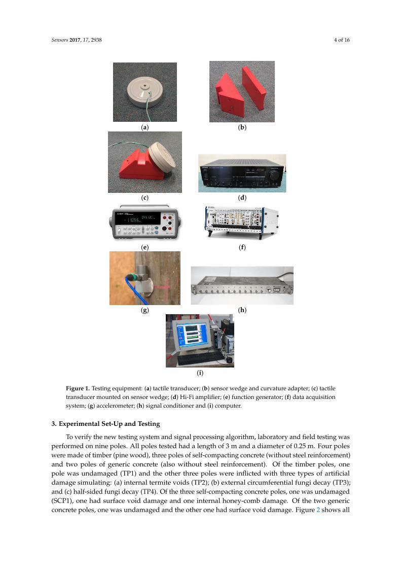
The testing equipment used for the experimental validation of the newly proposed testing systemis presented in Figure 1 and includes the following: (a) a tactile transducer for a symmetric andsynchronized narrow-band frequency excitation; (b) a sensor wedge (and curvature adapters) fordirecting the wave in the longitudinal direction of the structure; (c) a tactile transducer mountedon a sensor wedge; (d) a Hi-Fi amplifier for amplification and adjustment of the amplitude of theexcited wave; (e) a function generator for generation of the desired excitation waveform and frequency;(f) a data acquisition system; (h) accelerometers (PCB, model 352C34) with a frequency range of 0.5 Hzto 10,000 Hz for measuring the wave propagation along the structure; (g) a signal conditioner forsupplying the accelerometers with constant current; and (i) a computer for recording the data.

Sensors 2017, 17, 2938 4 of 16

Sensors 2017, 17, 2938 4 of 15

(a) (b)

(c) (d)

(e) (f)

(g) (h)

(i)

Figure 1. Testing equipment: (a) tactile transducer; (b) sensor wedge and curvature adapter; (c) tactile transducer mounted on sensor wedge; (d) Hi-Fi amplifier; (e) function generator; (f) data acquisition system; (g) accelerometer; (h) signal conditioner and (i) computer.

3. Experimental Set-Up and Testing

To verify the new testing system and signal processing algorithm, laboratory and field testing was performed on nine poles. All poles tested had a length of 3 m and a diameter of 0.25 m. Four poles were made of timber (pine wood), three poles of self-compacting concrete (without steel reinforcement) and two poles of generic concrete (also without steel reinforcement). Of the timber poles, one pole was undamaged (TP1) and the other three poles were inflicted with three types of artificial damage simulating: (a) internal termite voids (TP2); (b) external circumferential fungi decay (TP3); and (c) half-sided fungi decay (TP4). Of the three self-compacting concrete poles, one was undamaged (SCP1), one had surface void damage and one internal honey-comb damage. Of the two generic concrete poles, one was undamaged and the other one had surface void damage. Figure 2 shows all tested poles presenting dimensions and damage types. Figure 3 displays photos of some example damage cases. The pole identifier, material, damage type and dimensions of all nine tested poles are listed in Table 1.

Figure 1. Testing equipment: (a) tactile transducer; (b) sensor wedge and curvature adapter; (c) tactiletransducer mounted on sensor wedge; (d) Hi-Fi amplifier; (e) function generator; (f) data acquisitionsystem; (g) accelerometer; (h) signal conditioner and (i) computer.

3. Experimental Set-Up and Testing

To verify the new testing system and signal processing algorithm, laboratory and field testing wasperformed on nine poles. All poles tested had a length of 3 m and a diameter of 0.25 m. Four poleswere made of timber (pine wood), three poles of self-compacting concrete (without steel reinforcement)and two poles of generic concrete (also without steel reinforcement). Of the timber poles, onepole was undamaged (TP1) and the other three poles were inflicted with three types of artificialdamage simulating: (a) internal termite voids (TP2); (b) external circumferential fungi decay (TP3);and (c) half-sided fungi decay (TP4). Of the three self-compacting concrete poles, one was undamaged(SCP1), one had surface void damage and one internal honey-comb damage. Of the two genericconcrete poles, one was undamaged and the other one had surface void damage. Figure 2 shows all

Sensors 2017, 17, 2938 5 of 16

tested poles presenting dimensions and damage types. Figure 3 displays photos of some exampledamage cases. The pole identifier, material, damage type and dimensions of all nine tested poles arelisted in Table 1.Sensors 2017, 17, 2938 5 of 15

(a) (b) (c) (d) (e) (f) (g) (h) (i)

Figure 2. Dimensions and damage configurations of the tested poles in longitudinal and cross-sectional view: (a) undamaged timber pole, (b) timber pole with internal void damage, (c) timber pole with external circumferential cross-section loss damage, (d) timber poles with half-sided cross-section loss damage, (e) undamaged self-compacting concrete pole, (f) self-compacting concrete pole with surface void damage, (g) self-compacting concrete pole with internal honey-comb damage, (h) undamaged generic concrete pole, and (i) generic concrete pole with surface void damage.

(a) (b) (c) (d)

Figure 3. Examples of some damaged poles: (a) timber pole with internal void damage; (b) timber pole with external circumferential cross-section loss damage; (c) timber pole with half-sided cross-section loss damage and (d) self-compacting concrete pole with surface void damage.

Table 1. Pole identifier, material, damage type and dimensions of tested pole structures.

Identifier Material Damage Type Damage DimensionsTP1 Timber Undamaged - TP2 Timber Internal void damage Φ = 0.15 m, h = 0.7 m TP3 Timber External circumferential damage Φ = 0.15 m, h = 0.7 m TP4 Timber Half-sided cross-section loss damage w = 0.125 m, h = 0.7 m

SCP1 Self-compacting concrete Undamaged - SCP2 Self-compacting concrete Surface void damage wmax = 0.125 m, hmax = 0.4 m SCP3 Self-compacting concrete Internal honey-comb damage Φ = 0.2 m GCP1 Generic concrete Undamaged - GCP2 Generic concrete Surface void damage w = 0.125 m, h = 0.2 m

Figure 2. Dimensions and damage configurations of the tested poles in longitudinal and cross-sectionalview: (a) undamaged timber pole, (b) timber pole with internal void damage, (c) timber pole withexternal circumferential cross-section loss damage, (d) timber poles with half-sided cross-section lossdamage, (e) undamaged self-compacting concrete pole, (f) self-compacting concrete pole with surfacevoid damage, (g) self-compacting concrete pole with internal honey-comb damage, (h) undamagedgeneric concrete pole, and (i) generic concrete pole with surface void damage.

Sensors 2017, 17, 2938 5 of 15

(a) (b) (c) (d) (e) (f) (g) (h) (i)

Figure 2. Dimensions and damage configurations of the tested poles in longitudinal and cross-sectional view: (a) undamaged timber pole, (b) timber pole with internal void damage, (c) timber pole with external circumferential cross-section loss damage, (d) timber poles with half-sided cross-section loss damage, (e) undamaged self-compacting concrete pole, (f) self-compacting concrete pole with surface void damage, (g) self-compacting concrete pole with internal honey-comb damage, (h) undamaged generic concrete pole, and (i) generic concrete pole with surface void damage.

(a) (b) (c) (d)

Figure 3. Examples of some damaged poles: (a) timber pole with internal void damage; (b) timber pole with external circumferential cross-section loss damage; (c) timber pole with half-sided cross-section loss damage and (d) self-compacting concrete pole with surface void damage.

Table 1. Pole identifier, material, damage type and dimensions of tested pole structures.

Identifier Material Damage Type Damage DimensionsTP1 Timber Undamaged - TP2 Timber Internal void damage Φ = 0.15 m, h = 0.7 m TP3 Timber External circumferential damage Φ = 0.15 m, h = 0.7 m TP4 Timber Half-sided cross-section loss damage w = 0.125 m, h = 0.7 m

SCP1 Self-compacting concrete Undamaged - SCP2 Self-compacting concrete Surface void damage wmax = 0.125 m, hmax = 0.4 m SCP3 Self-compacting concrete Internal honey-comb damage Φ = 0.2 m GCP1 Generic concrete Undamaged - GCP2 Generic concrete Surface void damage w = 0.125 m, h = 0.2 m

Figure 3. Examples of some damaged poles: (a) timber pole with internal void damage; (b) timber polewith external circumferential cross-section loss damage; (c) timber pole with half-sided cross-sectionloss damage and (d) self-compacting concrete pole with surface void damage.

Sensors 2017, 17, 2938 6 of 16

Table 1. Pole identifier, material, damage type and dimensions of tested pole structures.

Identifier Material Damage Type Damage Dimensions

TP1 Timber Undamaged -TP2 Timber Internal void damage Φ = 0.15 m, h = 0.7 mTP3 Timber External circumferential damage Φ = 0.15 m, h = 0.7 mTP4 Timber Half-sided cross-section loss damage w = 0.125 m, h = 0.7 m

SCP1 Self-compacting concrete Undamaged -SCP2 Self-compacting concrete Surface void damage wmax = 0.125 m, hmax = 0.4 mSCP3 Self-compacting concrete Internal honey-comb damage Φ = 0.2 mGCP1 Generic concrete Undamaged -GCP2 Generic concrete Surface void damage w = 0.125 m, h = 0.2 m

All nine poles were tested with two types of setup configurations, that is: (1) in the laboratory(standing freely on a Styrofoam mat); and (2) in the field (with soil embedment and exposure toenvironmental conditions). The laboratory testing was executed at the German Federal Institute forMaterial Research and Testing (BAM) non-destructive testing laboratories of Division 8.2, and the fieldtesting at the BAM Test Site Technical Safety (BAM-TTS) in Horstwald. For all testing, four tactiletransducers were used as excitation sources and 12 accelerometers (A1 to A12) measured the waveresponse of the structure. The four tactile transducers were mounted to the sensor wedges via a screwconnection and were firmly attached to the pole structure at a height of 1.5 m in a ring formation withequal spacing using a ratchet strap. To allow full wave transmission from the sensor wedge to the pole,a thin layer of Vaseline was applied between the wedge and pole interface. The accelerometers wereattached to the pole using moulding clay. For both laboratory and field testing setup, all accelerometerswere attached in three rings with four accelerometers per ring. Sensor ring 1 was located 0.1 m belowthe excitation ring, and sensor rings 2 and 3 were distanced 0.3 m and 0.5 m below the excitationsource, respectively. For field testing, the poles were embedded in the ground with a soil embedmentof 1.0 m. As excitation force, continuous narrow-band sine wave signals with a frequency of 1 kHzwere induced simultaneously at all four tactile transducers. The wave response of the pole structureswas captured simultaneously by the 12 accelerometers with a sampling rate of 1 MHz and a recordingtime of 0.06 s. To generate multiple data sets, each pole configuration was tested 5 times. The detailedtest setup arrangements for both experimental and field testing are shown in Figure 4.

Sensors 2017, 17, 2938 6 of 15

All nine poles were tested with two types of setup configurations, that is: (1) in the laboratory (standing freely on a Styrofoam mat); and (2) in the field (with soil embedment and exposure to environmental conditions). The laboratory testing was executed at the German Federal Institute for Material Research and Testing (BAM) non-destructive testing laboratories of Division 8.2, and the field testing at the BAM Test Site Technical Safety (BAM-TTS) in Horstwald. For all testing, four tactile transducers were used as excitation sources and 12 accelerometers (A1 to A12) measured the wave response of the structure. The four tactile transducers were mounted to the sensor wedges via a screw connection and were firmly attached to the pole structure at a height of 1.5 m in a ring formation with equal spacing using a ratchet strap. To allow full wave transmission from the sensor wedge to the pole, a thin layer of Vaseline was applied between the wedge and pole interface. The accelerometers were attached to the pole using moulding clay. For both laboratory and field testing setup, all accelerometers were attached in three rings with four accelerometers per ring. Sensor ring 1 was located 0.1 m below the excitation ring, and sensor rings 2 and 3 were distanced 0.3 m and 0.5 m below the excitation source, respectively. For field testing, the poles were embedded in the ground with a soil embedment of 1.0 m. As excitation force, continuous narrow-band sine wave signals with a frequency of 1 kHz were induced simultaneously at all four tactile transducers. The wave response of the pole structures was captured simultaneously by the 12 accelerometers with a sampling rate of 1 MHz and a recording time of 0.06 s. To generate multiple data sets, each pole configuration was tested 5 times. The detailed test setup arrangements for both experimental and field testing are shown in Figure 4.

(a) (b) (c) (d) (e)

Figure 4. Laboratory and field testing set-up: (a) laboratory testing of timber pole; (b) laboratory testing of concrete pole; (c) field testing of timber pole; (d) field testing of concrete pole; and (e) labels and dimensions of test setup.

4. Signal Processing: Feature Extraction Using FFT and PCA

For signal processing, an advanced signal analysis algorithm is proposed, which extracts damage features from the wave signals of the accelerometer network for the condition assessment of

Figure 4. Laboratory and field testing set-up: (a) laboratory testing of timber pole; (b) laboratorytesting of concrete pole; (c) field testing of timber pole; (d) field testing of concrete pole; and (e) labelsand dimensions of test setup.

Sensors 2017, 17, 2938 7 of 16

4. Signal Processing: Feature Extraction Using FFT and PCA

For signal processing, an advanced signal analysis algorithm is proposed, which extracts damagefeatures from the wave signals of the accelerometer network for the condition assessment of bothtimber and concrete pole structures using FFT data and PCA. In the proposed method, first, time-seriesstress wave signals are recorded from the laboratory and field testing of the different pole structuresusing the new testing system. For the testing, the poles are excited with narrow-band continuous wavesignals in the shape of sine waves with an excitation frequency of 1 kHz. This frequency was chosen asit lies in the typical excitation range of traditional impact hammer testing. Second, the signals capturedfrom accelerometers of the same ring are summed up to generate a new signal sequence. This signalsummation is applied in order to suppress asymmetric wave components. Third, the newly generatedtime-domain signal sequence from each sensor ring is transferred to the frequency-domain usingFFT and subsequently mean FFT signals are calculated by averaging the FFTs from the three sensorrings. Fourth, to reduce measurement noise effects and the amount of feature data, PCA is adopted tocompress the mean FFT data. Finally, a selected number of the most dominant principal components(PCs) are chosen as damage specific indices distinguishing undamaged poles from different types ofdamaged poles. The detailed feature extraction procedure is presented in Figure 5.

Sensors 2017, 17, 2938 7 of 15

both timber and concrete pole structures using FFT data and PCA. In the proposed method, first, time-series stress wave signals are recorded from the laboratory and field testing of the different pole structures using the new testing system. For the testing, the poles are excited with narrow-band continuous wave signals in the shape of sine waves with an excitation frequency of 1 kHz. This frequency was chosen as it lies in the typical excitation range of traditional impact hammer testing. Second, the signals captured from accelerometers of the same ring are summed up to generate a new signal sequence. This signal summation is applied in order to suppress asymmetric wave components. Third, the newly generated time-domain signal sequence from each sensor ring is transferred to the frequency-domain using FFT and subsequently mean FFT signals are calculated by averaging the FFTs from the three sensor rings. Fourth, to reduce measurement noise effects and the amount of feature data, PCA is adopted to compress the mean FFT data. Finally, a selected number of the most dominant principal components (PCs) are chosen as damage specific indices distinguishing undamaged poles from different types of damaged poles. The detailed feature extraction procedure is presented in Figure 4.

Figure 5. Flow-chart of feature extraction based on FFT signals and PCA.

As an example of the summarized acceleration signals, Figure 6 presents a time-domain stress wave signal from sensor ring 3 of a timber pole with internal void damage tested in the laboratory. Signals from different sensor rings have similar wave patterns due to the continuous sine wave excitation (amplitude and frequency) with the exception of a phase shift resulting from the different ring positions with delayed up- and downward wave travel.

Figure 6. Original segmented time-domain acceleration signal from sensor ring 3 of a timber pole with internal void damage tested in the laboratory.

To extract damage-sensitive features from the measurement data, in the proposed method, the time-domain signals are transferred to the frequency domain using FFT. As an example, Figure 7 displays FFT data with a bandwidth of 0 to 5000 Hz of the four types of timber poles tested in the laboratory. It is noticeable that the energy distribution of the FFT signals from the intact pole is mainly concentrated around the 1 kHz frequency band (which is the excitation frequency of the transducers), while the response of the damaged poles contains higher amplitude harmonics at 2, 3 and 4 kHz. This suggests that the damage has introduced nonlinearities into the structure. In addition, different damage types produce different FFT amplitudes, in particular in the response at 1 kHz. These damage features can now be used by a classifier to identify the different types of damage.

Figure 5. Flow-chart of feature extraction based on FFT signals and PCA.

As an example of the summarized acceleration signals, Figure 6 presents a time-domain stresswave signal from sensor ring 3 of a timber pole with internal void damage tested in the laboratory.Signals from different sensor rings have similar wave patterns due to the continuous sine waveexcitation (amplitude and frequency) with the exception of a phase shift resulting from the differentring positions with delayed up- and downward wave travel.

Sensors 2017, 17, 2938 7 of 15

both timber and concrete pole structures using FFT data and PCA. In the proposed method, first, time-series stress wave signals are recorded from the laboratory and field testing of the different pole structures using the new testing system. For the testing, the poles are excited with narrow-band continuous wave signals in the shape of sine waves with an excitation frequency of 1 kHz. This frequency was chosen as it lies in the typical excitation range of traditional impact hammer testing. Second, the signals captured from accelerometers of the same ring are summed up to generate a new signal sequence. This signal summation is applied in order to suppress asymmetric wave components. Third, the newly generated time-domain signal sequence from each sensor ring is transferred to the frequency-domain using FFT and subsequently mean FFT signals are calculated by averaging the FFTs from the three sensor rings. Fourth, to reduce measurement noise effects and the amount of feature data, PCA is adopted to compress the mean FFT data. Finally, a selected number of the most dominant principal components (PCs) are chosen as damage specific indices distinguishing undamaged poles from different types of damaged poles. The detailed feature extraction procedure is presented in Figure 4.

Figure 5. Flow-chart of feature extraction based on FFT signals and PCA.

As an example of the summarized acceleration signals, Figure 6 presents a time-domain stress wave signal from sensor ring 3 of a timber pole with internal void damage tested in the laboratory. Signals from different sensor rings have similar wave patterns due to the continuous sine wave excitation (amplitude and frequency) with the exception of a phase shift resulting from the different ring positions with delayed up- and downward wave travel.

Figure 6. Original segmented time-domain acceleration signal from sensor ring 3 of a timber pole with internal void damage tested in the laboratory.

To extract damage-sensitive features from the measurement data, in the proposed method, the time-domain signals are transferred to the frequency domain using FFT. As an example, Figure 7 displays FFT data with a bandwidth of 0 to 5000 Hz of the four types of timber poles tested in the laboratory. It is noticeable that the energy distribution of the FFT signals from the intact pole is mainly concentrated around the 1 kHz frequency band (which is the excitation frequency of the transducers), while the response of the damaged poles contains higher amplitude harmonics at 2, 3 and 4 kHz. This suggests that the damage has introduced nonlinearities into the structure. In addition, different damage types produce different FFT amplitudes, in particular in the response at 1 kHz. These damage features can now be used by a classifier to identify the different types of damage.

Figure 6. Original segmented time-domain acceleration signal from sensor ring 3 of a timber pole withinternal void damage tested in the laboratory.

To extract damage-sensitive features from the measurement data, in the proposed method,the time-domain signals are transferred to the frequency domain using FFT. As an example, Figure 7displays FFT data with a bandwidth of 0 to 5000 Hz of the four types of timber poles tested in thelaboratory. It is noticeable that the energy distribution of the FFT signals from the intact pole is mainlyconcentrated around the 1 kHz frequency band (which is the excitation frequency of the transducers),while the response of the damaged poles contains higher amplitude harmonics at 2, 3 and 4 kHz.This suggests that the damage has introduced nonlinearities into the structure. In addition, differentdamage types produce different FFT amplitudes, in particular in the response at 1 kHz. These damagefeatures can now be used by a classifier to identify the different types of damage.

Sensors 2017, 17, 2938 8 of 16Sensors 2017, 17, 2938 8 of 15

(a) (b)

(c) (d)

Figure 7. Averaged fast Fourier transforms (FFTs) of wave signals from the three sensor rings of timber poles tested in the laboratory: (a) TP1; (b) TP2; (c) TP3; and (d) TP4.

If the full FFT data set is used as feature inputs for classifier training using machine learning techniques, it will result in slow training convergence and inefficient computations, since the full data set contains a vast amount of redundant information. Further, the FFT data contains disturbances from measurement noise, that are particularly present in field testing data, and which compromise the result accuracy. Due to these limitations, PCA is applied as an effective tool to filter noise and compress data by replacing the original FFTs with a small number of dominant PCs [12,13].

Pearson [14] originally developed the concept of PCA, which is based on the eigenvalue decomposition of the covariance matrix. PCA is a statistical method for achieving dimensionality reduction and is one of the most powerful multivariate data analysis techniques. Applying the concept of PCA, an original set of k variables is linearly transformed into a smaller set of n (n ≤ k) uncorrelated variables, the so-called principal components (PCs). The direction of the resulting eigenvectors represents the direction of the PCs and each PC is a linear combination of the original variables. After transformation, the PCs are weighted according to value of the corresponding eigenvalues. All the PCs are orthogonal to each other and form an orthogonal basis for the space of the data. So the first PC is weighted highest and has the largest eigenvalue. The corresponding first eigenvector represents the direction and amount of maximum variability of the original data set. The second PC is orthogonal to the first PC and represents the second most significant contribution in the data set, and so on [15]. By removing components that contribute least to the overall variance, the dimension of the original data set can drastically be reduced without significantly affecting the original data [16]. In addition to data reduction, PCA is also a powerful tool for filtering unwanted noise. As noise is a random feature that is not correlated with the global characteristics of the data set, it is represented by less significant PCs. Therefore, by ignoring PCs of low power, measurement noise is filtered.

Figure 7. Averaged fast Fourier transforms (FFTs) of wave signals from the three sensor rings of timberpoles tested in the laboratory: (a) TP1; (b) TP2; (c) TP3; and (d) TP4.

If the full FFT data set is used as feature inputs for classifier training using machine learningtechniques, it will result in slow training convergence and inefficient computations, since the full dataset contains a vast amount of redundant information. Further, the FFT data contains disturbances frommeasurement noise, that are particularly present in field testing data, and which compromise the resultaccuracy. Due to these limitations, PCA is applied as an effective tool to filter noise and compress databy replacing the original FFTs with a small number of dominant PCs [12,13].

Pearson [14] originally developed the concept of PCA, which is based on the eigenvaluedecomposition of the covariance matrix. PCA is a statistical method for achieving dimensionalityreduction and is one of the most powerful multivariate data analysis techniques. Applying the conceptof PCA, an original set of k variables is linearly transformed into a smaller set of n (n ≤ k) uncorrelatedvariables, the so-called principal components (PCs). The direction of the resulting eigenvectorsrepresents the direction of the PCs and each PC is a linear combination of the original variables.After transformation, the PCs are weighted according to value of the corresponding eigenvalues.All the PCs are orthogonal to each other and form an orthogonal basis for the space of the data.So the first PC is weighted highest and has the largest eigenvalue. The corresponding first eigenvectorrepresents the direction and amount of maximum variability of the original data set. The second PCis orthogonal to the first PC and represents the second most significant contribution in the data set,and so on [15]. By removing components that contribute least to the overall variance, the dimension ofthe original data set can drastically be reduced without significantly affecting the original data [16].In addition to data reduction, PCA is also a powerful tool for filtering unwanted noise. As noise is

Sensors 2017, 17, 2938 9 of 16

a random feature that is not correlated with the global characteristics of the data set, it is representedby less significant PCs. Therefore, by ignoring PCs of low power, measurement noise is filtered.

For this study, PCA transformation is applied to the FFT signals of the tested pole structures.As example, Figure 8 displays the individual and cumulative contributions of the first ten PCs of theFFTs of timber poles tested in (a) the laboratory and (b) the field. It can be seen that the first four PCscontain more than 99% contribution of all the information. So by only selecting a small number ofdominant PCs, the size of feature indices can be greatly reduced while maintaining the vast majorityof information, which is highly beneficial for the classifier training.

Sensors 2017, 17, 2938 9 of 15

For this study, PCA transformation is applied to the FFT signals of the tested pole structures. As example, Figure 8 displays the individual and cumulative contributions of the first ten PCs of the FFTs of timber poles tested in (a) the laboratory and (b) the field. It can be seen that the first four PCs contain more than 99% contribution of all the information. So by only selecting a small number of dominant PCs, the size of feature indices can be greatly reduced while maintaining the vast majority of information, which is highly beneficial for the classifier training.

(a) (b)

Figure 8. Contributions of the first ten principle components (PCs) of feature indices from timber pole specimens: (a) laboratory testing and (b) field testing.

To select the optimal number of PCs, which contain sufficient information for damage classification, an investigation on the effect of the different damage types to the PCs is conducted. Figure 9 presents the first ten PCs of FFT data of the four different timber poles tested in (a) the laboratory and (b) the field. Since each pole configuration was tested five times, five lines are plotted for each pole. It can be observed that the first four components show clearly distinguishable patterns for the different types of damage, which forms the basis of the proposed damage identification method. Further, for damage of the same type, the PCs obtained are of similar values, that is, in this study, the PCs are similar for the five tests of the same pole. Since the PCs from the fifth component onwards have only small contribution values, which indicate their negligible contributions, the first four dominant components are considered as suitable indices for subsequent damage classification. It is noted that PCA was applied separately to the laboratory and the field testing data, since the boundary conditions are substantially different (soil embedment vs. free standing). Hence, the derived PCs are of different values reflecting the different composition of structural features.

(a) (b)

Figure 9. First ten PCs of FFT data of timber poles with different damage conditions: (a) laboratory testing and (b) field testing.

1 2 3 4 5 6 7 8 9 10

-250

-200

-150

-100

-50

0

50

100

150

200

250

300

Prin

cipa

l com

pone

nt v

alue

Principal component index

TP1 TP2 TP3 TP4

1 2 3 4 5 6 7 8 9 10

-60

-30

0

30

60

90

120 TP1 TP2 TP3 TP4

Prin

cipa

l com

pone

nt v

alue

Principal component index

Figure 8. Contributions of the first ten principle components (PCs) of feature indices from timber polespecimens: (a) laboratory testing and (b) field testing.

To select the optimal number of PCs, which contain sufficient information for damageclassification, an investigation on the effect of the different damage types to the PCs is conducted.Figure 9 presents the first ten PCs of FFT data of the four different timber poles tested in(a) the laboratory and (b) the field. Since each pole configuration was tested five times, five lines areplotted for each pole. It can be observed that the first four components show clearly distinguishablepatterns for the different types of damage, which forms the basis of the proposed damage identificationmethod. Further, for damage of the same type, the PCs obtained are of similar values, that is, in thisstudy, the PCs are similar for the five tests of the same pole. Since the PCs from the fifth componentonwards have only small contribution values, which indicate their negligible contributions, the firstfour dominant components are considered as suitable indices for subsequent damage classification.It is noted that PCA was applied separately to the laboratory and the field testing data, since theboundary conditions are substantially different (soil embedment vs. free standing). Hence, the derivedPCs are of different values reflecting the different composition of structural features.

Figures 10–12 present the PC results of the different pole structures showing only the first andsecond PCs. For each pole condition, all five test results are presented. From the figures, it can be seenthat the PCs of the different pole types cluster together. This demonstrates that the selected indices areable to distinguish the different pole damage scenarios. It further shows that the proposed FFT andPCA-based signal processing method can effectively extract damage features from the wave signals.

Sensors 2017, 17, 2938 10 of 16

Sensors 2017, 17, 2938 9 of 15

For this study, PCA transformation is applied to the FFT signals of the tested pole structures. As example, Figure 8 displays the individual and cumulative contributions of the first ten PCs of the FFTs of timber poles tested in (a) the laboratory and (b) the field. It can be seen that the first four PCs contain more than 99% contribution of all the information. So by only selecting a small number of dominant PCs, the size of feature indices can be greatly reduced while maintaining the vast majority of information, which is highly beneficial for the classifier training.

(a) (b)

Figure 8. Contributions of the first ten principle components (PCs) of feature indices from timber pole specimens: (a) laboratory testing and (b) field testing.

To select the optimal number of PCs, which contain sufficient information for damage classification, an investigation on the effect of the different damage types to the PCs is conducted. Figure 9 presents the first ten PCs of FFT data of the four different timber poles tested in (a) the laboratory and (b) the field. Since each pole configuration was tested five times, five lines are plotted for each pole. It can be observed that the first four components show clearly distinguishable patterns for the different types of damage, which forms the basis of the proposed damage identification method. Further, for damage of the same type, the PCs obtained are of similar values, that is, in this study, the PCs are similar for the five tests of the same pole. Since the PCs from the fifth component onwards have only small contribution values, which indicate their negligible contributions, the first four dominant components are considered as suitable indices for subsequent damage classification. It is noted that PCA was applied separately to the laboratory and the field testing data, since the boundary conditions are substantially different (soil embedment vs. free standing). Hence, the derived PCs are of different values reflecting the different composition of structural features.

(a) (b)

Figure 9. First ten PCs of FFT data of timber poles with different damage conditions: (a) laboratory testing and (b) field testing.

1 2 3 4 5 6 7 8 9 10

-250

-200

-150

-100

-50

0

50

100

150

200

250

300Pr

inci

pal c

ompo

nent

val

ue

Principal component index

TP1 TP2 TP3 TP4

1 2 3 4 5 6 7 8 9 10

-60

-30

0

30

60

90

120 TP1 TP2 TP3 TP4

Prin

cipa

l com

pone

nt v

alue

Principal component index

Figure 9. First ten PCs of FFT data of timber poles with different damage conditions: (a) laboratorytesting and (b) field testing.

Sensors 2017, 17, 2938 10 of 15

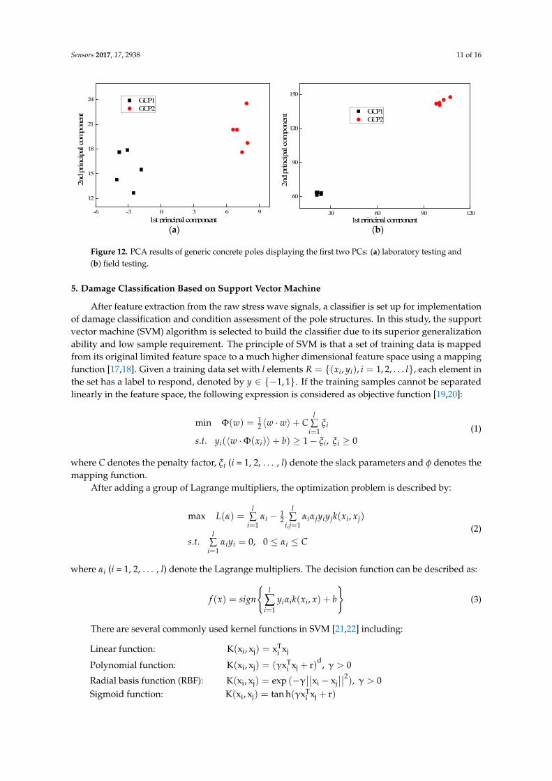
Figures 10–12 present the PC results of the different pole structures showing only the first and second PCs. For each pole condition, all five test results are presented. From the figures, it can be seen that the PCs of the different pole types cluster together. This demonstrates that the selected indices are able to distinguish the different pole damage scenarios. It further shows that the proposed FFT and PCA-based signal processing method can effectively extract damage features from the wave signals.

(a) (b)

Figure 10. First ten PCs of FFT data of timber poles with different damage conditions: (a) laboratory testing and (b) field testing.

(a) (b)

Figure 11. Principal component analysis (PCA) results of self-compacting concrete poles displaying the first two PCs: (a) laboratory testing and (b) field testing.

(a) (b)

Figure 12. PCA results of generic concrete poles displaying the first two PCs: (a) laboratory testing and (b) field testing.

40 80 120 160 200

-200

-160

-120

-80

-40 TP1 TP2 TP3 TP4

2nd

prin

cipa

l com

pone

nt

1st principal component

30 60 90 120

30

60

90

120 TP1 TP2 TP3 TP4

2nd

pinc

ipal

com

pone

nt

1st principal component

36 40 44 48 52

24

28

32

36

SCP1 SCP2 SCP3

2nd

prin

cipa

l com

pone

nt

1st principal component

-80 -60 -40 -20 0

-20

-16

-12

-8 SCP1 SCP2 SCP3

2nd

prin

cipa

l com

pone

nt

1st principal component

-6 -3 0 3 6 9

12

15

18

21

24 GCP1 GCP2

2nd

prin

cipa

l com

pone

nt

1st principal component

30 60 90 120

60

90

120

150

GCP1 GCP2

2nd

prin

cipa

l com

pone

nt

1st principal component

Figure 10. First ten PCs of FFT data of timber poles with different damage conditions: (a) laboratorytesting and (b) field testing.

Sensors 2017, 17, 2938 10 of 15

Figures 10–12 present the PC results of the different pole structures showing only the first and second PCs. For each pole condition, all five test results are presented. From the figures, it can be seen that the PCs of the different pole types cluster together. This demonstrates that the selected indices are able to distinguish the different pole damage scenarios. It further shows that the proposed FFT and PCA-based signal processing method can effectively extract damage features from the wave signals.

(a) (b)

Figure 10. First ten PCs of FFT data of timber poles with different damage conditions: (a) laboratory testing and (b) field testing.

(a) (b)

Figure 11. Principal component analysis (PCA) results of self-compacting concrete poles displaying the first two PCs: (a) laboratory testing and (b) field testing.

(a) (b)

Figure 12. PCA results of generic concrete poles displaying the first two PCs: (a) laboratory testing and (b) field testing.

40 80 120 160 200

-200

-160

-120

-80

-40 TP1 TP2 TP3 TP4

2nd

prin

cipa

l com

pone

nt

1st principal component

30 60 90 120

30

60

90

120 TP1 TP2 TP3 TP4

2nd

pinc

ipal

com

pone

nt

1st principal component

36 40 44 48 52

24

28

32

36

SCP1 SCP2 SCP3

2nd

prin

cipa

l com

pone

nt

1st principal component

-80 -60 -40 -20 0

-20

-16

-12

-8 SCP1 SCP2 SCP3

2nd

prin

cipa

l com

pone

nt

1st principal component

-6 -3 0 3 6 9

12

15

18

21

24 GCP1 GCP2

2nd

prin

cipa

l com

pone

nt

1st principal component

30 60 90 120

60

90

120

150

GCP1 GCP2

2nd

prin

cipa

l com

pone

nt

1st principal component

Figure 11. Principal component analysis (PCA) results of self-compacting concrete poles displayingthe first two PCs: (a) laboratory testing and (b) field testing.

Sensors 2017, 17, 2938 11 of 16

Sensors 2017, 17, 2938 10 of 15

Figures 10–12 present the PC results of the different pole structures showing only the first and second PCs. For each pole condition, all five test results are presented. From the figures, it can be seen that the PCs of the different pole types cluster together. This demonstrates that the selected indices are able to distinguish the different pole damage scenarios. It further shows that the proposed FFT and PCA-based signal processing method can effectively extract damage features from the wave signals.

(a) (b)

Figure 10. First ten PCs of FFT data of timber poles with different damage conditions: (a) laboratory testing and (b) field testing.

(a) (b)

Figure 11. Principal component analysis (PCA) results of self-compacting concrete poles displaying the first two PCs: (a) laboratory testing and (b) field testing.

(a) (b)

Figure 12. PCA results of generic concrete poles displaying the first two PCs: (a) laboratory testing and (b) field testing.

40 80 120 160 200

-200

-160

-120

-80

-40 TP1 TP2 TP3 TP4

2nd

prin

cipa

l com

pone

nt

1st principal component

30 60 90 120

30

60

90

120 TP1 TP2 TP3 TP4

2nd

pinc

ipal

com

pone

nt

1st principal component

36 40 44 48 52

24

28

32

36

SCP1 SCP2 SCP3

2nd

prin

cipa

l com

pone

nt

1st principal component

-80 -60 -40 -20 0

-20

-16

-12

-8 SCP1 SCP2 SCP3

2nd

prin

cipa

l com

pone

nt

1st principal component

-6 -3 0 3 6 9

12

15

18

21

24 GCP1 GCP2

2nd

prin

cipa

l com

pone

nt

1st principal component

30 60 90 120

60

90

120

150

GCP1 GCP2

2nd

prin

cipa

l com

pone

nt

1st principal component

Figure 12. PCA results of generic concrete poles displaying the first two PCs: (a) laboratory testing and(b) field testing.

5. Damage Classification Based on Support Vector Machine

After feature extraction from the raw stress wave signals, a classifier is set up for implementationof damage classification and condition assessment of the pole structures. In this study, the supportvector machine (SVM) algorithm is selected to build the classifier due to its superior generalizationability and low sample requirement. The principle of SVM is that a set of training data is mappedfrom its original limited feature space to a much higher dimensional feature space using a mappingfunction [17,18]. Given a training data set with l elements R = {(xi, yi), i = 1, 2, . . . l}, each element inthe set has a label to respond, denoted by y ∈ {−1, 1}. If the training samples cannot be separatedlinearly in the feature space, the following expression is considered as objective function [19,20]:

min Φ(w) = 12 〈w · w〉+ C

l∑

i=1ξi

s.t. yi(〈w ·Φ(xi)〉+ b) ≥ 1− ξi, ξi ≥ 0(1)

where C denotes the penalty factor, ξi (i = 1, 2, . . . , l) denote the slack parameters and φ denotes themapping function.

After adding a group of Lagrange multipliers, the optimization problem is described by:

max L(α) =l

∑i=1

αi − 12

l∑

i,j=1αiαjyiyjk(xi, xj)

s.t.l

∑i=1

αiyi = 0, 0 ≤ αi ≤ C(2)

where αi (i = 1, 2, . . . , l) denote the Lagrange multipliers. The decision function can be described as:

f (x) = sign

{l

∑i=1

yiαik(xi, x) + b

}(3)

There are several commonly used kernel functions in SVM [21,22] including:

Linear function: K(xi, xj) = xTi xj

Polynomial function: K(xi, xj) = (γxTi xj + r)d, γ > 0

Radial basis function (RBF): K(xi, xj) = exp (−γ∣∣∣∣xi − xj

∣∣∣∣2), γ > 0Sigmoid function: K(xi, xj) = tan h(γxT

i xj + r)

Sensors 2017, 17, 2938 12 of 16

In this work, all of the kernel functions above are used to train the SVM multi-classifier andthe results of the different kernel functions are eventually compared against each other to select theoptimal kernel function.

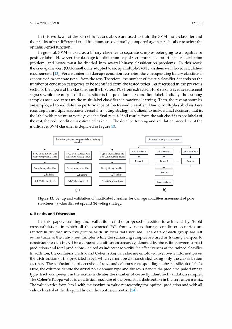
In general, SVM is used as a binary classifier to separate samples belonging to a negative orpositive label. However, the damage identification of pole structures is a multi-label classificationproblem, and hence must be divided into several binary classification problems. In this work,the one-against-rest (OAR) method is adopted to set up multiple SVM classifiers with fewer calculationrequirements [23]. For a number of i damage condition scenarios, the corresponding binary classifier isconstructed to separate type i from the rest. Therefore, the number of the sub classifier depends on thenumber of condition categories to be identified from the tested poles. As discussed in the previoussections, the inputs of the classifier are the first four PCs from extracted FFT data of wave measurementsignals while the output of the classifier is the pole damage condition label. Initially, the trainingsamples are used to set up the multi-label classifier via machine learning. Then, the testing samplesare employed to validate the performance of the trained classifier. Due to multiple sub classifiersresulting in multiple assessment results, a voting strategy is utilized to make a final decision; that is,the label with maximum votes gives the final result. If all results from the sub classifiers are labels ofthe rest, the pole condition is estimated as intact. The detailed training and validation procedure of themulti-label SVM classifier is depicted in Figure 13.

Sensors 2017, 17, 2938 12 of 15

(a) (b)

Figure 13. Set up and validation of multi-label classifier for damage condition assessment of pole

structures: (a) classifier set up, and (b) voting strategy.

6. Results and Discussion

In this paper, training and validation of the proposed classifier is achieved by 5-fold cross-

validation, in which all the extracted PCs from various damage condition scenarios are randomly

divided into five groups with uniform data volume. The data of each group are left out in turns as

the validation samples while the remaining samples are used as training samples to construct the

classifier. The averaged classification accuracy, denoted by the ratio between correct predictions and

total predictions, is used as indicator to verify the effectiveness of the trained classifier. In addition,

the confusion matrix and Cohen’s Kappa value are employed to provide information on the

distribution of the predicted label, which cannot be demonstrated using only the classification

accuracy. The confusion matrix consists of rows and columns corresponding to the classification

labels. Here, the columns denote the actual pole damage type and the rows denote the predicted pole

damage type. Each component in the matrix indicates the number of correctly identified validation

samples. The Cohen’s Kappa value is a statistical measure of the prediction distribution in the

confusion matrix. The value varies from 0 to 1 with the maximum value representing the optimal

prediction and with all values located at the diagonal line in the confusion matrix [24].

(a) (b)

Figure 14. Confusion matrices of support vector machine (SVM) classifiers constructed from data of

timber pole laboratory testing using: (a) the RBF kernel function; and (b) the linear kernel function.

As an example, Figure 14a,b present the results of the confusion matrix for the timber pole data

from the laboratory testing using (a) the RBF function and (b) the linear kernel function, respectively.

The results illustrate that the trained classifier can effectively separate the undamaged pole from the

damaged poles with internal, external circumferential and half-sided damage with a classification

accuracy of 100%. However, for the damage type identification, the classifier with the RBF kernel

function outperforms the linear kernel function in the classification of the external circumferential

Extracted principal components from training

samples

Type 1 data and rest data

with corresponding labels

Type 2 data and rest data

with corresponding labels

Type n data and rest data

with corresponding labels

Set up binary classifier Set up binary classifier Set up binary classifier

Sub SVM classifier 1 Sub SVM classifier 2 Sub SVM classifier n

Training Training Training

Extracted principal components

Sub classifier 1 Sub classifier 2 Sub classifier n......

Voting

Pole condition

Result 1 Result 2 Result n......

5

100%

0

0.0%

0

0.0%

0

0.0%

0

0.0%

0

0.0%

0

0.0%

5

100%

5

100%

0

0.0%

0

0.0%

0

0.0%

0

0.0%

0

0.0%

0

0.0%

5

100%

No damage Internal damage

External round damage

Half-sided damage

No

dam

ag

eIn

tern

al

dam

age

Ex

tern

al r

ou

nd

d

amag

eH

alf-

sid

ed

dam

age

100%

0.0%

100%

0.0%

100%

0.0%

100%

0.0%

Predicted type

Pra

ctic

al

typ

e

TPR/FNR

5

100%

0

0.0%

0

0.0%

0

0.0%

0

0.0%

0

0.0%

0

0.0%

5

100%

3

60%

0

0.0%

0

0.0%

2

40%

0

0.0%

1

20%

0

0.0%

4

80%

No damage Internal damage

External round damage

Half-sided damage

No

dam

ag

eIn

tern

al

dam

age

Exte

rnal

ro

un

d

dam

age

Hal

f-si

ded

d

amag

e

100%

0.0%

100%

0.0%

60%

40%

80%

20%

Predicted type

Pra

ctic

al

typ

e

TPR/FNR

Figure 13. Set up and validation of multi-label classifier for damage condition assessment of polestructures: (a) classifier set up, and (b) voting strategy.

6. Results and Discussion

In this paper, training and validation of the proposed classifier is achieved by 5-foldcross-validation, in which all the extracted PCs from various damage condition scenarios arerandomly divided into five groups with uniform data volume. The data of each group are leftout in turns as the validation samples while the remaining samples are used as training samples toconstruct the classifier. The averaged classification accuracy, denoted by the ratio between correctpredictions and total predictions, is used as indicator to verify the effectiveness of the trained classifier.In addition, the confusion matrix and Cohen’s Kappa value are employed to provide information onthe distribution of the predicted label, which cannot be demonstrated using only the classificationaccuracy. The confusion matrix consists of rows and columns corresponding to the classification labels.Here, the columns denote the actual pole damage type and the rows denote the predicted pole damagetype. Each component in the matrix indicates the number of correctly identified validation samples.The Cohen’s Kappa value is a statistical measure of the prediction distribution in the confusion matrix.The value varies from 0 to 1 with the maximum value representing the optimal prediction and with allvalues located at the diagonal line in the confusion matrix [24].

Sensors 2017, 17, 2938 13 of 16

As an example, Figure 14a,b present the results of the confusion matrix for the timber pole datafrom the laboratory testing using (a) the RBF function and (b) the linear kernel function, respectively.The results illustrate that the trained classifier can effectively separate the undamaged pole from thedamaged poles with internal, external circumferential and half-sided damage with a classificationaccuracy of 100%. However, for the damage type identification, the classifier with the RBF kernelfunction outperforms the linear kernel function in the classification of the external circumferential andthe half-sided damage. It can further be seen that the latter classifier predicts 40% of the poles withexternal circumferential damage as intact poles and 20% of the poles with half-sided damage as poleswith internal damage.

Sensors 2017, 17, 2938 12 of 15

(a) (b)

Figure 13. Set up and validation of multi-label classifier for damage condition assessment of pole

structures: (a) classifier set up, and (b) voting strategy.

6. Results and Discussion

In this paper, training and validation of the proposed classifier is achieved by 5-fold cross-

validation, in which all the extracted PCs from various damage condition scenarios are randomly

divided into five groups with uniform data volume. The data of each group are left out in turns as

the validation samples while the remaining samples are used as training samples to construct the

classifier. The averaged classification accuracy, denoted by the ratio between correct predictions and

total predictions, is used as indicator to verify the effectiveness of the trained classifier. In addition,

the confusion matrix and Cohen’s Kappa value are employed to provide information on the

distribution of the predicted label, which cannot be demonstrated using only the classification

accuracy. The confusion matrix consists of rows and columns corresponding to the classification

labels. Here, the columns denote the actual pole damage type and the rows denote the predicted pole

damage type. Each component in the matrix indicates the number of correctly identified validation

samples. The Cohen’s Kappa value is a statistical measure of the prediction distribution in the

confusion matrix. The value varies from 0 to 1 with the maximum value representing the optimal

prediction and with all values located at the diagonal line in the confusion matrix [24].

(a) (b)

Figure 14. Confusion matrices of support vector machine (SVM) classifiers constructed from data of

timber pole laboratory testing using: (a) the RBF kernel function; and (b) the linear kernel function.

As an example, Figure 14a,b present the results of the confusion matrix for the timber pole data

from the laboratory testing using (a) the RBF function and (b) the linear kernel function, respectively.

The results illustrate that the trained classifier can effectively separate the undamaged pole from the

damaged poles with internal, external circumferential and half-sided damage with a classification

accuracy of 100%. However, for the damage type identification, the classifier with the RBF kernel

function outperforms the linear kernel function in the classification of the external circumferential

Extracted principal components from training

samples

Type 1 data and rest data

with corresponding labels

Type 2 data and rest data

with corresponding labels

Type n data and rest data

with corresponding labels

Set up binary classifier Set up binary classifier Set up binary classifier

Sub SVM classifier 1 Sub SVM classifier 2 Sub SVM classifier n

Training Training Training

Extracted principal components

Sub classifier 1 Sub classifier 2 Sub classifier n......

Voting

Pole condition

Result 1 Result 2 Result n......

5

100%

0

0.0%

0

0.0%

0

0.0%

0

0.0%

0

0.0%

0

0.0%

5

100%

5

100%

0

0.0%

0

0.0%

0

0.0%

0

0.0%

0

0.0%

0

0.0%

5

100%

No damage Internal damage

External round damage

Half-sided damage

No

dam

ag

eIn

tern

al

dam

age

Ex

tern

al r

ou

nd

d

amag

eH

alf-

sid

ed

dam

age

100%

0.0%

100%

0.0%

100%

0.0%

100%

0.0%

Predicted type

Pra

ctic

al

typ

e

TPR/FNR

5

100%

0

0.0%

0

0.0%

0

0.0%

0

0.0%

0

0.0%

0

0.0%

5

100%

3

60%

0

0.0%

0

0.0%

2

40%

0

0.0%

1

20%

0

0.0%

4

80%

No damage Internal damage

External round damage

Half-sided damage

No

dam

ag

eIn

tern

al

dam

age

Ex

tern

al r

ou

nd

dam

age

Hal

f-si

ded

d

amag

e

100%

0.0%

100%

0.0%

60%

40%

80%

20%

Predicted type

Pra

ctic

al

typ

e

TPR/FNR

Figure 14. Confusion matrices of support vector machine (SVM) classifiers constructed from data oftimber pole laboratory testing using: (a) the RBF kernel function; and (b) the linear kernel function.

Figure 15a shows the classification accuracies of all pole structures for different kernel functioncases. The results demonstrate that the RBF function gives the best classification results compared to allother employed kernel functions. Using the RBF function can achieve classification accuracies of over80%, meeting the practical requirement of pole structure condition assessment. Figure 15b displaysthe associated Cohen’s Kappa values of the classifiers with different kernel functions. Again, the RBFfunction outperforms the other kernel function. Overall, the results in Figure 15 show that the linear,polynomial and sigmoid functions can neither provide a statistically better classification accuracy nora better Kappa value compared to the RBF function, which achieves classification accuracy results of92.5% ± 7.5% and a Cohen’s Kappa value range of [0.8, 1.0].

Sensors 2017, 17, 2938 13 of 15

and the half-sided damage. It can further be seen that the latter classifier predicts 40% of the poles with external circumferential damage as intact poles and 20% of the poles with half-sided damage as poles with internal damage.

Figure 15a shows the classification accuracies of all pole structures for different kernel function cases. The results demonstrate that the RBF function gives the best classification results compared to all other employed kernel functions. Using the RBF function can achieve classification accuracies of over 80%, meeting the practical requirement of pole structure condition assessment. Figure 15b displays the associated Cohen’s Kappa values of the classifiers with different kernel functions. Again, the RBF function outperforms the other kernel function. Overall, the results in Figure 15 show that the linear, polynomial and sigmoid functions can neither provide a statistically better classification accuracy nor a better Kappa value compared to the RBF function, which achieves classification accuracy results of 92.5% ± 7.5% and a Cohen’s Kappa value range of [0.8, 1.0].

(a) (b)

Figure 15. Statistical indicators for all tested pole specimen of the classifiers with different kernel functions: (a) classification accuracy; and (b) Cohen’s Kappa value.

Finally, the classification results for all pole specimens tested based on 5-fold cross validation are summarized in Table 2. It can be seen that the trained SVM-based multi-classifiers are able to identify the undamaged pole cases with 100% classification accuracy. Although several cases of damaged poles are inaccurately predicted, the models still achieve a very high performance (over 80%), which meets the condition assessment requirements of pole asset managements.

Table 2. Summary of classification results for all pole specimens tested in both the laboratory and the field.

Classification Accuracy (Correct/Total)

Type Undamaged

(TP1) Internal Damage (TP2) External Round (TP3) Half Sided

(TP4)

TP Lab 100% (5/5) 100% (5/5) 100% (5/5) 100% (5/5)

Field 100% (5/5) 100% (5/5) 80% (4/5) 80% (4/5)

Type Undamaged (SCP1)

Surface void (SCP2) Internal

honey-comb (SCP3)

SCP Lab 100% (5/5) 80% (4/5) 100% (5/5)

Field 100% (5/5) 80% (4/5) 80% (4/5) Type Undamaged (GP1) Surface void (GP2)

GP Lab 100% (5/5) 100% (5/5) Field 100% (5/5) 80% (4/5)

7. Conclusions

Linear Polynomial RBF Sigmoid0.75

0.80

0.85

0.90

0.95

1.00

Clas

sific

atio

n ac

cura

cy

Linear Polynomial RBF Sigmoid

0.6

0.7

0.8

0.9

1.0

Cohe

n's K

appa

val

ue

Figure 15. Statistical indicators for all tested pole specimen of the classifiers with different kernelfunctions: (a) classification accuracy; and (b) Cohen’s Kappa value.

Sensors 2017, 17, 2938 14 of 16

Finally, the classification results for all pole specimens tested based on 5-fold cross validation aresummarized in Table 2. It can be seen that the trained SVM-based multi-classifiers are able to identifythe undamaged pole cases with 100% classification accuracy. Although several cases of damaged polesare inaccurately predicted, the models still achieve a very high performance (over 80%), which meetsthe condition assessment requirements of pole asset managements.

Table 2. Summary of classification results for all pole specimens tested in both the laboratory andthe field.

Classification Accuracy (Correct/Total)

Type Undamaged(TP1) Internal Damage (TP2) External Round (TP3) Half Sided

(TP4)

TPLab 100% (5/5) 100% (5/5) 100% (5/5) 100% (5/5)

Field 100% (5/5) 100% (5/5) 80% (4/5) 80% (4/5)

Type Undamaged(SCP1) Surface void (SCP2)

Internalhoney-comb

(SCP3)

SCPLab 100% (5/5) 80% (4/5) 100% (5/5)

Field 100% (5/5) 80% (4/5) 80% (4/5)

Type Undamaged (GP1) Surface void (GP2)

GPLab 100% (5/5) 100% (5/5)

Field 100% (5/5) 80% (4/5)

7. Conclusions

This paper presented a novel testing system for foundation piles and utility poles usinga network of tactile transducers and accelerometers alongside an advanced signal processing techniquefor condition assessment and damage classification. The innovative testing system uses tactiletransducers in a ring configuration to excite narrow-band frequency stress waves, in order to generateaxisymmetric guided waves and thereby reduce the appearance of multi-wave types and modestypically encountered with broadband hammer excitation. The proposed advanced signal processingmethod utilized fast Fourier transform (FFT) signals and principal component analysis (PCA) toprocess measured stress wave signals containing specific damage signal features. The support vectormachine (SVM) algorithm was used to set up multi-label classifiers for the prediction of pole damageconditions. To validate the new testing system and proposed signal analysis technique, different typesof pole structures (timber and concrete poles) with various damage scenarios were tested in both thelaboratory and the field (with soil embedment), inducing continuous sine wave excitation signals.The results of the advanced signal processing method demonstrated that the damage condition of thetested poles can be identified from extracted damage features using FFT data and PCA, and that theSVM multi-label classifier with the RBF kernel function can provide very good classification resultswith an optimal accuracy of 92.5% ± 7.5% and a Kappa value in the range of 0.8 and 1. In futurework, the new narrow-band frequency excitation system will be tested in combination with theproposed advanced signal analysis technique for different excitation wave forms and frequencies,and it will be applied to actual in-situ foundation piles and utility poles with natural defects to verifythe performance for practical engineering applications.

Acknowledgments: This work was supported by the UTS International Research Development Scheme and theATN-DAAD collaborative researcher exchange grant. The technical and laboratory staff of Division 8.2 of theFederal Institute for Materials Research and Testing, Germany (BAM) is greatly thanked for assisting with theequipment setup and testing. In particular, Matthias Behrens is thanked for designing and manufacturing thesensor wedges, Andreas Zoëga and Frank Mielentz for supporting the equipment setup, and Marco Lange andSean Smith for their assistance with the laboratory and field testing.

Sensors 2017, 17, 2938 15 of 16

Author Contributions: Ulrike Dackermann developed the new testing system and conceived, designed andperformed the laboratory and field experiments; Yang Yu developed the signal processing methodology andanalyzed the data; Ulrike Dackermann and Yang Yu wrote the paper; Ernst Niederleithinger contributed to thedevelopment of the testing system and the experimental testing; Jianchun Li and Herbert Wiggenhauser providedessential mentoring that lead to the development of the proposed testing system.

Conflicts of Interest: The authors declare no conflict of interest.

References

1. Stepinski, T.; Uhl, T.; Staszewski, W. Advanced Structural Damage Detection—From Theory to EngineeringApplications; John Wiley & Sons, Ltd.: New York, NY, USA, 2013.

2. Tanasoiu, V.; Micleaa, C.; Tanasoiua, C. Nondestructive testing techniques and piezoelectric ultrasonicstransducers for wood and built in wooden structures. J. Optoelectron. Adv. Mater. 2002, 4, 949–957.

3. Dackermann, U.; Skinner, B.; Li, J. Guided wave–based condition assessment of in situ timber utility polesusing machine learning algorithms. Struct. Health Monit. 2014, 13, 374–388. [CrossRef]

4. Dackermann, U.; Yu, Y.; Li, J.; Niederleithinger, E.; Wiggenhauser, H. A new non-destructive testing systembased on narrow-band frequency excitation for the condition assessment of pole structures using frequencyresponse functions and principle component analysis. In Proceedings of the International SymposiumNon-Destructive Testing in Civil Engineering (NDT-CE 2015), Berlin, Germany, 15–17 September 2015.

5. Ertel, J.-P.; Niederleithinger, E.; Grohmann, M. Advances in pile integrity testing. Near Surf. Geophys.2016, 14, 503–512. [CrossRef]

6. Dackermann, U.; Crews, K.; Kasal, B.; Li, J.; Riggio, M.; Rinn, F.; Tannert, T. In situ assessment of structuraltimber using stress-wave measurements. Mater. Struct. 2013, 47, 787–803. [CrossRef]

7. Hertlein, B.; Davis, A. Nondestructive Testing of Deep Foundations; John Wiley & Sons, Ltd.: Chichester,UK, 2006.

8. Niederleithinger, E.; Wolf, J.; Mielentz, F.; Wiggenhauser, H.; Pirskawetz, S. Embedded ultrasonic transducersfor active and passive concrete monitoring. Sensors 2015, 15, 9756–9772. [CrossRef] [PubMed]

9. Li, J.; Subhani, M.; Samali, B. Determination of embedment depth of timber poles and piles using wavelettransform. Adv. Struct. Eng. 2012, 15, 759–770. [CrossRef]

10. Cui, D.-M.; Yan, W.; Wang, X.-Q.; Lu, L.-M. Towards intelligent interpretation of low strain pile integritytesting results using machine learning techniques. Sensors 2017, 17, 2443. [CrossRef] [PubMed]

11. Alleyne, D.N.; Cawley, P. The excitation of lamb waves in pipes using dry-coupled piezoelectric transducers.J. Nondestruct. Eval. 1996, 15, 11–20. [CrossRef]

12. Bianchini, A. Pavement maintenance planning at the network level with principal component analysis.J. Infrastruct. Syst. 2014, 20, 04013013. [CrossRef]

13. Li, J.; Dackermann, U.; Xu, Y.-L.; Samali, B. Damage identification in civil engineering structures utilizingPCA-compressed residual frequency response functions and neural network ensembles. Struct. Control.Health Monit. 2011, 18, 207–226. [CrossRef]

14. Pearson, K. On lines and planes of closest fit to systems of points in space. Philos. Mag. 1901, 2, 559–572.[CrossRef]

15. Tang, J. Frequency response based damage detection using principal component analysis. In Proceedingsof the IEEE International Conference on Information Acquisition, Hong Kong and Macau, China,27 June–3 July 2005; pp. 407–412.

16. Zang, C.; Imregun, M. Combined neural network and reduced FRF techniques for slight damage detectionusing measured response data. Arch. Appl. Mech. (Ing. Arch.) 2001, 71, 525–536. [CrossRef]

17. Zhang, X.; Chen, X.; He, Z. An aco-based algorithm for parameter optimization of support vector machines.Expert. Syst. Appl. 2010, 37, 6618–6628. [CrossRef]

18. Ao, H.; Cheng, J.; Zheng, J.; Truong, T.K. Roller bearing fault diagnosis method based on chemical reactionoptimization and support vector machine. J. Comput. Civil. Eng. 2015, 29, 04014077. [CrossRef]

19. Park, S.; Inman, D.J.; Lee, J.-J.; Yun, C.-B. Piezoelectric sensor-based health monitoring of railroad tracksusing a two-step support vector machine classifier. J. Infrastruct. Syst. 2008, 14, 80–88. [CrossRef]

20. Vapnik, V.N. Statistical Learning Theory; John Wiley & Sons, Inc.: New York, NY, USA, 1998.21. Lam, K.-C.; Lam, M.C.-K.; Wang, D. Efficacy of using support vector machine in a contractor prequalification

decision model. J. Comput. Civil. Eng. 2010, 24, 273–280. [CrossRef]

Sensors 2017, 17, 2938 16 of 16

22. Su, J.; Wang, X.; Liang, Y.; Chen, B. Ga-based support vector machine model for the prediction of monthlyreservoir storage. J. Hydrol. Eng. 2014, 19, 1430–1437. [CrossRef]

23. Qian, H.; Mao, Y.; Xiang, W.; Wang, Z. Recognition of human activities using svm multi-class classifier.Pattern Recogn. Lett. 2010, 31, 100–111. [CrossRef]

24. Witten, I.H.; Frank, E.; Hall, M.A. Data Mining: Practical Machine Learning Tools and Techniques, 3rd ed.;Morgan Kaufmann: San Francisco, CA, USA, 2011.

© 2017 by the authors. Licensee MDPI, Basel, Switzerland. This article is an open accessarticle distributed under the terms and conditions of the Creative Commons Attribution(CC BY) license (http://creativecommons.org/licenses/by/4.0/).