Concept Study and Design of a

New Torque Calibration Rig

Albin Lidgren

Automotive Engineering, bachelor's level

2017

Luleå University of Technology

Department of Engineering Sciences and Mathematics

i

Abstract

When buying a new car today, the customer often expects to get a vehiclewith high quality. Each vehicle or engine should therefore be checked toassure quality. The same goes for clutches and couplings. A powerful en-gine becomes useless when a clutch slips. Reliable torque measurement istherefore essential to the automotive industry. The herewith Bachelor thesisproposes a new torque calibration rig for online torque measurement in coup-ling applications.The concept encompasses a servo motor with its associated electronics, agearbox to create the high torques (3 kNm), a reference torque transducer,and mounting elements or adapters. From the concept generation phase, thethesis includes CAD-models of the torque calibration rig with mathematicalmodels leading to the calculation of the measurement uncertainty of the cal-ibration system.This work was performed at BorgWarner PowerDrive Systems AB in Landsk-rona during eight weeks; the two remaining weeks were completed in Lulea.

ii

iii

Sammanfattning

Nar man koper en ny bil, forvantar sig koparen hog kvalite. Varje fordoneller motor bor darfor vara kollad for att forsakra kvaliten. Det ar samma forkopplingar och lamellpaket. En kraftfull motor blir obrukbar nar kopplingenslirar. Palitlig vridmomentmatning ar darfor grundlaggande for bilindustrin.Detta kandidatexamen foreslar darfor en ny vridmomentkalibreringsrigg forvridmomentmatning i kopplingssystem i kopplingsapplikationer.I konceptet ingar en servomotor med tillhorande elektronik for styrning, envaxellada for att kunna skapa sa hoga moment som 3 kNm, referenssenorsom kalibreringen utgar ifran, vaxellads- och sensorfasten samt tillhorandeadaptrar sa att allt passar ihop. Utover konceptgenereringen har aven enmatosakerhetsberakning av kalibreringssystemet utforts. Det ar vid dennaberakning som mest tid har lagt under arbetet for att finna och utfora enkorrekt analys och berakning av matosakerhet.Arbetet har under atta veckor utforts pa BorgWarner PowerDrive SystemsAB i Landskrona, de tva resterande veckorna har utforts i Lulea.

iv

v

Acknowledgements

I would like to start by thanking my family who always is there for me. Iwant to say thanks to all teachers and professors at Lulea University of Tech-nology’s Automotive Engineering program, especially to Jan van Deventerfor his guidance throughout this thesis. I would like to say thanks to BjornHelander at BorgWarner PDS in Landskrona who has been my supervisorand to all other colleagues at the TTT-department.

vi

vii

Contents

Abstract ii

Sammanfattning iv

Acknowledgements vi

List of Figures xi

List of Tables xiii

Glossary xiv

1 Introduction 11.1 Background . . . . . . . . . . . . . . . . . . . . . . . . . . . . 1

1.1.1 Definition of Torque . . . . . . . . . . . . . . . . . . . 11.2 The Company . . . . . . . . . . . . . . . . . . . . . . . . . . . 2

1.2.1 Engine Group . . . . . . . . . . . . . . . . . . . . . . . 21.2.2 Drivetrain Group . . . . . . . . . . . . . . . . . . . . . 21.2.3 BorgWarner PowerDrive Systems . . . . . . . . . . . . 3

1.3 The Product . . . . . . . . . . . . . . . . . . . . . . . . . . . . 31.3.1 The Introduction to Generation V Clutch-Pack Coupling 4

1.4 The Problem . . . . . . . . . . . . . . . . . . . . . . . . . . . 51.5 The Purpose . . . . . . . . . . . . . . . . . . . . . . . . . . . . 61.6 Project Boundaries . . . . . . . . . . . . . . . . . . . . . . . . 7

2 Theory 92.1 Introduction of Measurements . . . . . . . . . . . . . . . . . . 92.2 Explanation of important expressions related to Measurements 10

2.2.1 Repeatability . . . . . . . . . . . . . . . . . . . . . . . 10

viii

2.2.2 Confidence Level . . . . . . . . . . . . . . . . . . . . . 102.2.3 Calibration . . . . . . . . . . . . . . . . . . . . . . . . 102.2.4 Adjustment . . . . . . . . . . . . . . . . . . . . . . . . 11

2.3 Measurement Uncertainty . . . . . . . . . . . . . . . . . . . . 112.3.1 Calculation of Measurement Uncertainty . . . . . . . . 112.3.2 Torque Transducer Measurement Uncertainty . . . . . 15

3 Method 183.1 Generating Concepts . . . . . . . . . . . . . . . . . . . . . . . 18

3.1.1 Specifications . . . . . . . . . . . . . . . . . . . . . . . 183.1.2 Torque Transducer . . . . . . . . . . . . . . . . . . . . 193.1.3 Gearbox . . . . . . . . . . . . . . . . . . . . . . . . . . 193.1.4 Motor . . . . . . . . . . . . . . . . . . . . . . . . . . . 193.1.5 Prop shaft . . . . . . . . . . . . . . . . . . . . . . . . . 193.1.6 Adapters . . . . . . . . . . . . . . . . . . . . . . . . . . 203.1.7 Mountings . . . . . . . . . . . . . . . . . . . . . . . . . 203.1.8 Electronic encapsulation . . . . . . . . . . . . . . . . . 223.1.9 Torque Limiter . . . . . . . . . . . . . . . . . . . . . . 22

3.2 Software . . . . . . . . . . . . . . . . . . . . . . . . . . . . . . 233.3 Calculation of Measurement Uncertainty . . . . . . . . . . . . 24

3.3.1 Parameters of the application . . . . . . . . . . . . . . 243.3.2 Method to calculate the measurement uncertainty . . . 25

4 Results 284.1 Measurement Uncertainty of the Torque Transducer . . . . . . 284.2 The Concepts (A & B) . . . . . . . . . . . . . . . . . . . . . . 30

4.2.1 Concept A - Gearbox from NORD . . . . . . . . . . . 304.2.2 Concept B - Gearbox from Siemens . . . . . . . . . . . 314.2.3 Shaft fixation . . . . . . . . . . . . . . . . . . . . . . . 344.2.4 Safety . . . . . . . . . . . . . . . . . . . . . . . . . . . 364.2.5 Cost analysis . . . . . . . . . . . . . . . . . . . . . . . 36

5 Discussion 38

6 Conclusion 41

7 Further work 43

A Requirement Specifications 45

ix

B Existing Rigs 48

C Concepts 52C.1 Concept A . . . . . . . . . . . . . . . . . . . . . . . . . . . . . 52C.2 Concept B . . . . . . . . . . . . . . . . . . . . . . . . . . . . . 55C.3 Adapters . . . . . . . . . . . . . . . . . . . . . . . . . . . . . . 59C.4 Adapters . . . . . . . . . . . . . . . . . . . . . . . . . . . . . . 61

D Project Planning 67D.1 Project plan . . . . . . . . . . . . . . . . . . . . . . . . . . . . 67D.2 Risk Analysis . . . . . . . . . . . . . . . . . . . . . . . . . . . 69D.3 Gantt . . . . . . . . . . . . . . . . . . . . . . . . . . . . . . . 71

Bibliography 72

x

List of Figures

1.1 Different setups using some of BorgWarner’s drivetrain products. 31.2 Example of a driveline with a Generation V coupling, the setup

is called “Hang on rear” [12]. . . . . . . . . . . . . . . . . . . . 41.3 Exploded view of a Generation V coupling [11]. . . . . . . . . 5

2.1 Parasitic loads - axial force Fa, lateral force Fr and bendingmoment Mb . . . . . . . . . . . . . . . . . . . . . . . . . . . . 16

2.2 Example of static forces applied on a beam. . . . . . . . . . . 17

3.1 Distance between mounting holes in to the floor. . . . . . . . . 213.2 Mounting for torque transducer with possibilities to adjust the

position in every direction. . . . . . . . . . . . . . . . . . . . 223.3 Torque limiter used in the application for safety [22]. . . . . . 23

4.1 Concept A from side view. . . . . . . . . . . . . . . . . . . . 314.2 Simulated displacements on mountings for NORD concept. . 324.3 Simulated stress (von Mises) on mountings for NORD concept. 324.4 Concept B from side view. . . . . . . . . . . . . . . . . . . . 334.5 Simulated displacements on mountings for Siemens concept. . 334.6 Simulated stress (von Mises) on mountings for Siemens concept.

. . . . . . . . . . . . . . . . . . . . . . . . . . . . . . . . . . . 344.7 Example of a shaft mounted to the fixation and adapters for

other shafts. . . . . . . . . . . . . . . . . . . . . . . . . . . . 35

A.1 Mind map to get an easier overview of the torque calibrationrig requirements. . . . . . . . . . . . . . . . . . . . . . . . . . 47

B.1 Drawing of steel plates in rig room with holes. . . . . . . . . 50B.2 Steel plate in rig room without dimensions. . . . . . . . . . . 51

xi

C.1 View from transducer and shaft side. . . . . . . . . . . . . . . 52C.2 View from servo motor and transducer side . . . . . . . . . . . 53C.3 View from shaft side. . . . . . . . . . . . . . . . . . . . . . . . 53C.4 View from above . . . . . . . . . . . . . . . . . . . . . . . . . 54C.5 Simulated displacements on mountings for NORD concept. . 54C.6 Simulated stress (von Mises) on mountings for NORD concept. 55C.7 View from transducer and shaft side. . . . . . . . . . . . . . . 56C.8 View from servo motor and transducer side . . . . . . . . . . . 56C.9 View from shaft side. . . . . . . . . . . . . . . . . . . . . . . . 57C.10 View from above . . . . . . . . . . . . . . . . . . . . . . . . . 57C.11 Simulated displacements on mountings for concept B. . . . . 58C.12 Simulated stress (von Mises) on mountings for concept B. . . 58C.13 Fixation for shafts, different adapters and an example shaft. . 59C.14 Shaft fixation viewed from above. . . . . . . . . . . . . . . . 60C.15 Adapter from 108 mm to 68 mm. . . . . . . . . . . . . . . . . 61C.16 Adapter from 108 mm to 74 mm. . . . . . . . . . . . . . . . . 62C.17 Adapter from 108 mm to 86 mm. . . . . . . . . . . . . . . . . 63C.18 Adapter for 108 mm at the fixation. . . . . . . . . . . . . . . 64C.19 Adapter between HOWDON and T12 (130 mm hole picture),

with recessed bolt holes. . . . . . . . . . . . . . . . . . . . . . 65C.20 Adapter between T12 (130 mm) and HOWDON, with recessed

bolt holes. . . . . . . . . . . . . . . . . . . . . . . . . . . . . 66

xii

List of Tables

2.1 Table of a methodical arrangement of quantity, estimate, stand-ard uncertainty, probability distribution, sensitivity coefficientand contribution the the standard uncertainty [19]. . . . . . . 14

2.2 Table of different coverage factors for normal distribution withcorresponding confidence interval. . . . . . . . . . . . . . . . . 15

3.1 The most vital parameters from the Appendix RequirementSpecifications. . . . . . . . . . . . . . . . . . . . . . . . . . . . 19

3.2 Measurement Uncertainty Parameters from the data sheet andapplication (Fieldbuses/ Frequency output). . . . . . . . . . . 25

4.1 Calculation of worst case scenario Measurement Uncertaintyof a HBM T12 Torque Transducer in laboratory environment. 29

4.2 Dimensions of the concepts. All measuremens are in milli-meters and kilograms. . . . . . . . . . . . . . . . . . . . . . . 34

4.3 Cost analysis of concepts. All prices are in SEK ex. VAT. . . . 37

xiii

Glossary

ABS Anti Block SystemCAD Computer Aided DesignESC Electronic Stability ControlFEM Finite Element MethodPa SI-unit for Pressure [N/m2]τ Torque [Nm]Yaw-rate Rotation per time unit around an objects Z-axis [rad/sec]

xiv

xv

Chapter 1

Introduction

This introduction gives a background to the thesis conducted at BorgWarnerPowerDrive Systems AB in Landskrona. This thesis is a part of the Auto-motive Engineering program at Lulea University of Technology. This reportis written for people with an engineering background.

1.1 Background

This thesis has a red thread around the subjects Torque, Measurements andTorque Measurements.The issue being addressed here is the correct meas-urement of torque with reference to international standards. This sectionintroduces the subject of torque, how it is defined and who discovered it.Later in this report, the idea of measurements is introduced.The concept of torque can be traced all the way back to Archimedes and hisstudies with levers [1], this was around 230 BC [2].

1.1.1 Definition of Torque

Torque is defined as: “the cross product of the distance vector, r, (the dis-tance from the pivot point to the point where force is applied) and the forcevector, f .” [3] Equation 1.1 shows the correct mathematical representation.

τ = r × f (1.1)

Torque is measured in Newton-meter [Nm].

1

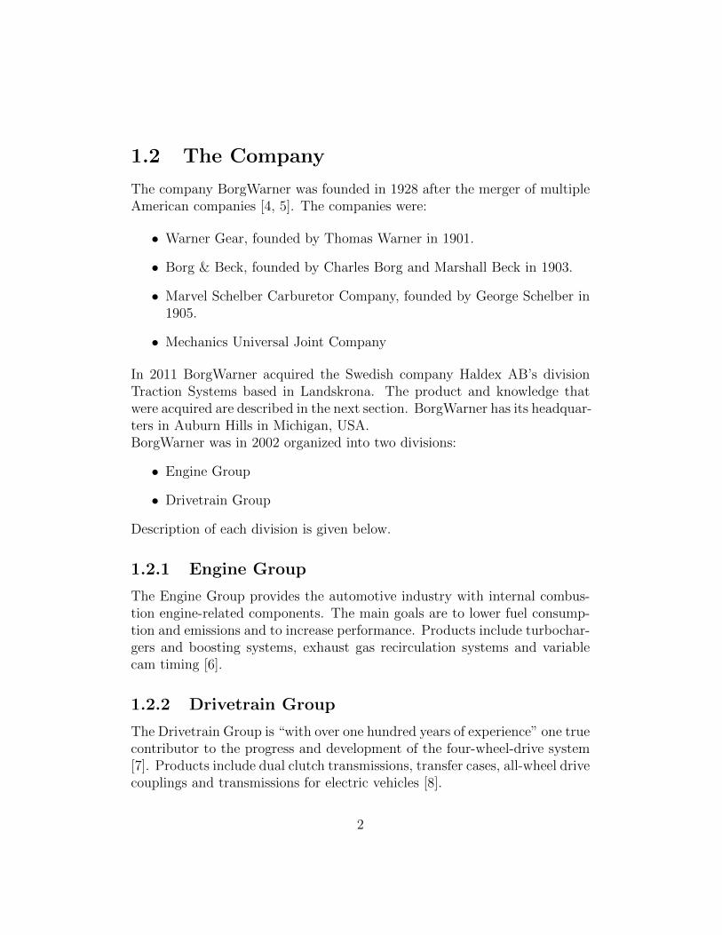
1.2 The Company

The company BorgWarner was founded in 1928 after the merger of multipleAmerican companies [4, 5]. The companies were:

• Warner Gear, founded by Thomas Warner in 1901.

• Borg & Beck, founded by Charles Borg and Marshall Beck in 1903.

• Marvel Schelber Carburetor Company, founded by George Schelber in1905.

• Mechanics Universal Joint Company

In 2011 BorgWarner acquired the Swedish company Haldex AB’s divisionTraction Systems based in Landskrona. The product and knowledge thatwere acquired are described in the next section. BorgWarner has its headquar-ters in Auburn Hills in Michigan, USA.BorgWarner was in 2002 organized into two divisions:

• Engine Group

• Drivetrain Group

Description of each division is given below.

1.2.1 Engine Group

The Engine Group provides the automotive industry with internal combus-tion engine-related components. The main goals are to lower fuel consump-tion and emissions and to increase performance. Products include turbochar-gers and boosting systems, exhaust gas recirculation systems and variablecam timing [6].

1.2.2 Drivetrain Group

The Drivetrain Group is “with over one hundred years of experience” one truecontributor to the progress and development of the four-wheel-drive system[7]. Products include dual clutch transmissions, transfer cases, all-wheel drivecouplings and transmissions for electric vehicles [8].

2

1.2.3 BorgWarner PowerDrive Systems

BorgWarner PowerDrive Systems has its origin in America and its devel-opment in the American and Asian automotive industry. To get into theEuropean automotive industry the Swedish company Haldex ABs divisionHaldex Traction Division was acquired in the beginning of 2011. HaldexTraction Division was developing, testing and manufacturing all-wheel-drivesystems for the European automotive industry. They have for example twotest facilities located in Sweden, one in Ljungbyhed near the plant in Land-skrona and another one in Arjeplog where they test their components duringwintertime in cold climate. Even prior to the purchase of ,the Traction Di-vision, BorgWarner had a good reputation in the automotive industry formaking solid all-wheel-drive systems. After the acquisition, the TractionDivision become a part of the Drivetrain Group at BorgWarner [9].

1.3 The Product

BorgWarners PowerDrive Systems products are found in several differentsetups, see examples in Figure 1.1.

Figure 1.1: Different setups using some of BorgWarner’s drivetrain products.

As shown in Figure 1.1 BorgWarner has many different solutions regard-ing torque vectoring and all-wheel-drive systems. In all these solutions andsystems above, the common factor is the Generation V coupling [10].

3

1.3.1 The Introduction to Generation V Clutch-PackCoupling

The Generation V coupling is as the name implies the fifth generation of thecoupling. Figure 1.2 shows the most common usage of the Gen V coupling[11].

Figure 1.2: Example of a driveline with a Generation V coupling, the setupis called “Hang on rear” [12].

The torque that is generated by the engine and is transferred via the drivelineto the wheels, which makes the car move forward. The driveline is everythingbetween the engine and the wheels. In most cases the driveline starts witha gearbox (manual or automatic), then comes a transmission, which dividesthe torque to the front- and back-wheels. From the transmission three driveshafts are attached, two for the front wheels and one prop shaft that transfersthe torque to the clutch-packs incoming axle. Torque is transferred from theclutch output axle via the final drive, the differential and then to the rearwheels [13].

4

Figure 1.3: Exploded view of a Generation V coupling [11].

The operation of the Gen V coupling begins at that the input flange, seeFigure 1.3, which is spun around by the prop shaft from the transmission.This makes the inner clutch plates rotate, but not the outer ones until thepiston pressures together the clutch plates. The outer plates are connected tothe outgoing axel of the coupling. The piston starts to pressurize the plateswhen the Centrifugal Electro-Hydraulic Actuator and the Axial Piston Pumphave build up a hydraulic pressure and the Control Module has given thesignal to send torque through the coupling to the rear wheels. The ControlModule calculates its signals from the car’s Yaw-rate, ABS-system, throttleposition, ESC-system and many more signals. The calculated results areready in microseconds.

1.4 The Problem

The problem that BorgWarner PowerDrive Systems had was that their torquesensors are fixed mounted to the test rigs, which were making the calibrationprocess time consuming and expensive. Earlier the calibration process weredangerous and not that accurate. The earlier calibration process were madewith a long rod used as a lever with different weights at different length from

5

the center. This procedure was very dangerous due to the fact that the rodkept on failing under high torque loads. When the rod failed, yes when notif, and the operators were in the work area surrounding the rod it could haveended very bad for the operator and even for the surrounding equipment.Today’s method is safer but is much more expensive. Today’s calibrationprocess starts with that the sensors are unmounted from the rig and thensent to an external company, which does the calibration. This unmounting,mounting and shipment is unwanted and expensive therefore, BorgWarnerwants to build there own torque calibration rig. With this torque calibrationrig, it is possible that the sensors retain mounted onto the existing rig. Thecalibration needs to be done against another torque sensor which is traceableagainst a national norms. BorgWarner needs to prove that their sensors arecalibrated against a national norms on their verified samples. The calibra-tion need to be traced to international standards. After the calibration aneventual adjustment to the sensor made.

1.5 The Purpose

The purpose of this thesis is to design a concept of a new torque calibrationrig that can ensure that the sensors measures the correct torque comparedto a national normal. A national norm is a standard calibrated at a certifiedcalibrator, e.g. RISE (former SP). If a sensor failed the calibration, all themeasurements done after the last calibration are invalid due to the fact thatit is impossible to tell if the sensor ever has been incorrect and when it stopmeasuring right. Therefore BorgWarner wants to, in a relatively simple way,calibrate their sensors often without needing to unmount the sensors fromthe rigs. The calibration needs to be done without missing out on accuracyor repeatability.

6

1.6 Project Boundaries

The thesis is like every bachelor thesis very short in terms of working time,ten weeks, which only eight of these are to be executed in Landskrona. Due tothat fact this thesis does not cover all the way through the process of concept,implementation and calibration of the new torque calibration rig. Instead itcovers the process of multiple concepts including concept studies, sharp bidsfrom manufacturers of transmissions and motors, and CAD models of theconcepts. The short period of shall will lead BorgWarner to order, build, testand implement this torque calibration rig by themselves. In the CAD modelssome simple strength of materials calculations are made (Finite ElementMethod-analysis and simulations). One extension of this thesis is that twodifferent presentations will be done, one at BorgWarner in Landskrona andone at Lulea University of Technology. This is necessary due to the distancebetween Landskrona and Lulea.

7

8

Chapter 2

Theory

This chapter covers the theory around the thesis. The theory goes into depthabout torque measurements and measurement uncertainty.

2.1 Introduction of Measurements

Why is measurements important today? Today humans keep track of everything,from the length of our body to the time it takes to get home with the bus. Itstarts when we are just a few years old and start to count (measure) how oldwe are or how many days it is until our birthday. Then we start to keep trackof time so that we do not miss the train or the bus. We measure when weare in the kitchen making dinner or a cake. The measurements in our livescontinue, our health could be measured by weight, blood pressure, pulse etc.Has measurements always been important for the humankind? In the be-ginning of measurements the body was used to measure, one example of anold unit is a ‘cubit’, which is the length of the arm from the elbow to thetip of the finger or units like a ‘foot’ [14]. This old length measurement isnot very accurate due to that no humans are alike, which makes this meas-urements dependent of who made it. The introduction of the units that isused today for measurements happened during the French Revolution. Onthe 22nd of June in 1799, two platinum standards representing the kilogramand the metre were displayed at the Archives de la Republique in Paris. Thistwo standards are seen as the first step to the development of the Interna-tional System of Units (SI) [15]. Today the unit meter is measured by thethe length of the path travelled by light in vacuum during a time interval of

9

1/299 792 458 of a second [16].

2.2 Explanation of important expressions re-

lated to Measurements

Here is a short explanation of expression often seen together with measure-ments and measurement uncertainty.

2.2.1 Repeatability

“Closeness of the agreement between repeated measurements of the same prop-erty under the same conditions” [17].Repeatability is the measurement process attribute to detain equal resultduring multiple measurements. The repeatability is one of the factors whichaffects the Measurement Uncertainty, see section Measurement Uncertainty.

2.2.2 Confidence Level

“The number (e.g. 95 %) expressing the degree of confidence in a result”[17].The confidence level tells the level of confidence in the result that the meas-urand is within the boundaries. The confidence level should, if possible, bestated as a probability. For example 95 % of all measurements are withinthe boundaries a and b.

2.2.3 Calibration

“Operation that, under specified conditions, in a first step, establishes a rela-tion between the quantity values with measurement uncertainties provided bymeasurement standards and corresponding indications with associated meas-urement uncertainties and, in a second step, uses this information to estab-lish a relation for obtaining a measurement result from an indication ” [18].Calibration of an instrument is a comparison between a known traceablestandard and the instruments measured value. The standard is a knownquantity, for example “exactly” 1.0000 kg.

10

2.2.4 Adjustment

“Set of operations carried out on a measuring system so that it providesprescribed indications corresponding to given values of a quantity to be meas-ured” [18]. Adjustment of this malfunction, see section Calibration, is some-thing else but it is needed for the instruments function. Adjustment is alsoknown as compensation.

2.3 Measurement Uncertainty

Measurement uncertainty is some kind of gray area surrounding the meas-urement result. How big this area is can be dependent of many factors, likethe human factor, environmental condition or the method of measurement.For example, if two different persons would measure a length of a stick witha measuring tape they could hold the tape differently and the measuringtape could have been stretched. Measurement uncertainty is a non-negativeparameter that belongs to the result of the measurement. This uncertaintydescribes the distribution of values that reasonably could be connected withthe result [19].

2.3.1 Calculation of Measurement Uncertainty

This section gives the necessary guidance to perform the calculation of meas-urement uncertainty. In calibration situations, it is usually only one meas-urand or output quantity Y . This measurand is dependent often of multipleinput quantities Xi (i = 1, 2, ..., N). The input quantities effect on the outputquantity is shown in equation 2.1. Input quantities can be everything fromhuman factors, if its measurable, to temperature deviation and non-linearity.

Y = f(X1, X2, . . . , XN) (2.1)

By using the estimations of the input quantities, xi, instead of the value Xi inequation 2.1 is an estimation, y, of the measurand Y obtained, see equation2.2.

y = f(x1, x2, . . . , xN) (2.2)

In evaluation of measurement uncertainty there is two different types of meth-ods, type A and type B. Evaluation method type A is based of statisticalanalysis on an observation series. In this case the measurement uncertainty

11

is the standard deviation of the mean by an average of the observation seriesor an appropriate regression analysis. Evaluation method type B is based onother methods than the statistical analysis. In this case it is based on sci-entific judgment using all of the relevant information available, for examplemanufacturer’s specifications (data sheets) or data provided in calibrationand other reports.

Type A evaluation of standard uncertainty

Type A is applicable if multiple independent observations have been made forone specific input quantity under unchanged circumstances. If the number ofobservations made is high enough there will be a spread of values obtained.An assumption of the repeatedly measured input quantity Xi is the quantityQ. The number of independent observations of Q is n, (n > 1). To calculatethe arithmetic mean or average of the estimation, of the quantity Q, qj (j =1, 2, . . . , n). qj is the individual observed values of the estimated quantity q.This is displayed in equation 2.3.

q =1

n

n∑j=1

qj (2.3)

The standard uncertainty u(qj) is to be associated with the qj through theestimated standard deviation of the arithmetic mean, seen in equation 2.4.

u(qj) = s(Qj) =

√√√√ 1

n(n− 1)

n∑k=1

(qj − qj)2 (2.4)

Type B evaluation of standard uncertainty

Type B is, like previous stated, based on other methods than a statisticalanalysis. There are three different types of cases to use type B, this threecases must by distinguished:

(i) If only one value for the quantity Xi is known, e.g. a reference valuefrom literature, a single measured value or a correction value, then thisvalue will be used for xi. If the standard uncertainty u(xi) is givenfor the value xi then this value is used. If the standard uncertainty is

12

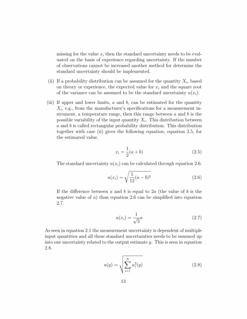
missing for the value xi then the standard uncertainty needs to be eval-uated on the basis of experience regarding uncertainty. If the numberof observations cannot be increased another method for determine thestandard uncertainty should be implemented.

(ii) If a probability distribution can be assumed for the quantity Xi, basedon theory or experience, the expected value for xi and the square rootof the variance can be assumed to be the standard uncertainty u(xi).

(iii) If upper and lower limits, a and b, can be estimated for the quantityXi, e.g., from the manufacturer’s specifications for a measurement in-strument, a temperature range, then this range between a and b is thepossible variability of the input quantity Xi. This distribution betweena and b is called rectangular probability distribution. This distributiontogether with case (ii) gives the following equation, equation 2.5, forthe estimated value.

xi =1

2(a+ b) (2.5)

The standard uncertainty u(xi) can be calculated through equation 2.6.

u(xi) =

√1

12(a− b)2 (2.6)

If the difference between a and b is equal to 2a (the value of b is thenegative value of a) than equation 2.6 can be simplified into equation2.7.

u(xi) =1√3a (2.7)

As seen in equation 2.1 the measurement uncertainty is dependent of multipleinput quantities and all these standard uncertainties needs to be summed upinto one uncertainty related to the output estimate y. This is seen in equation2.8.

u(y) =

√√√√ N∑i=1

u2i (y) (2.8)

13

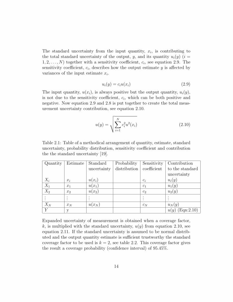
The standard uncertainty from the input quantity, xi, is contributing tothe total standard uncertainty of the output, y, and its quantity ui(y) (i =1, 2, . . . , N) together with a sensitivity coefficient, ci, see equation 2.9. Thesensitivity coefficient, ci, describes how the output estimate y is affected byvariances of the input estimate xi.

ui(y) = ciu(xi) (2.9)

The input quantity, u(xi), is always positive but the output quantity, ui(y),is not due to the sensitivity coefficient, ci, which can be both positive andnegative. Now equation 2.9 and 2.8 is put together to create the total meas-urement uncertainty contribution, see equation 2.10.

u(y) =

√√√√ N∑i=1

c2iu2(xi) (2.10)

Table 2.1: Table of a methodical arrangement of quantity, estimate, standarduncertainty, probability distribution, sensitivity coefficient and contributionthe the standard uncertainty [19].

Quantity

Xi

Estimate

xi

Standarduncertainty

u(xi)

Probabilitydistribution

Sensitivitycoefficient

ci

Contributionto the standarduncertaintyui(y)

X1 x1 u(x1) c1 u1(y)X2 x2 u(x2) c2 u2(y)...

......

......

XN xN u(xN) cN uN(y)Y y u(y) (Eqn:2.10)

Expanded uncertainty of measurement is obtained when a coverage factor,k, is multiplied with the standard uncertainty, u(y) from equation 2.10, seeequation 2.11. If the standard uncertainty is assumed to be normal distrib-uted and the output quantity estimate is sufficient trustworthy the standardcoverage factor to be used is k = 2, see table 2.2. This coverage factor givesthe result a coverage probability (confidence interval) of 95.45%.

14

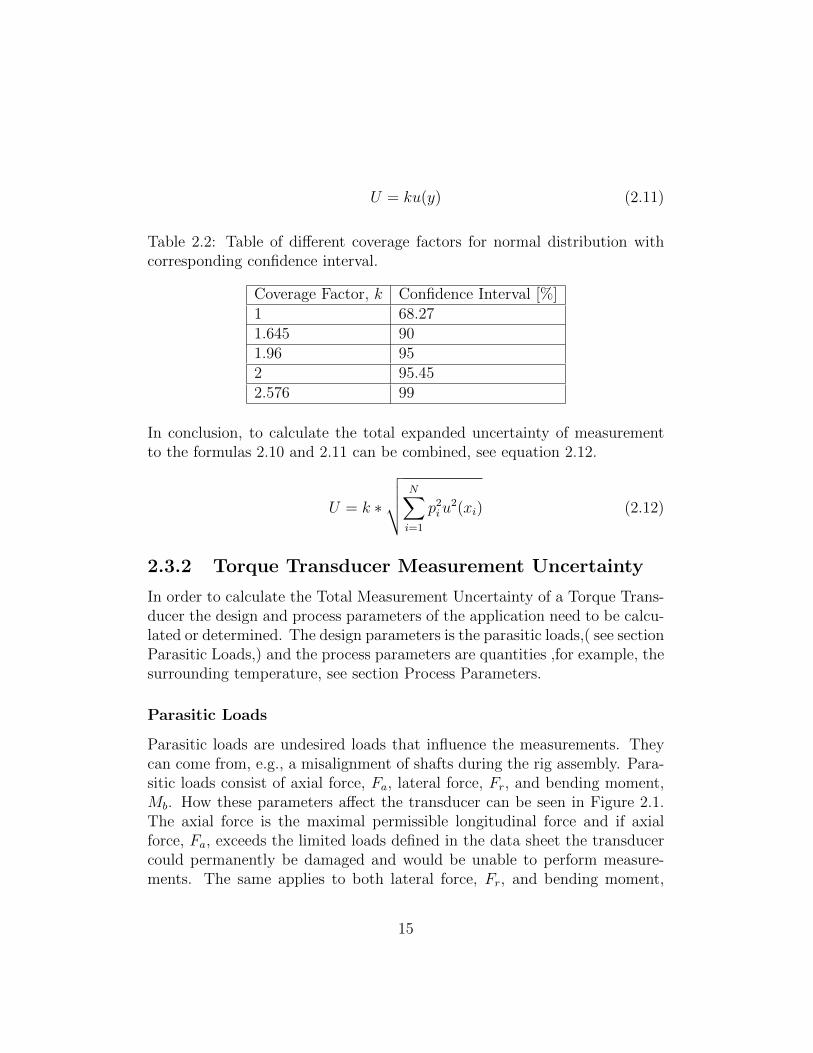
U = ku(y) (2.11)

Table 2.2: Table of different coverage factors for normal distribution withcorresponding confidence interval.

Coverage Factor, k Confidence Interval [%]1 68.271.645 901.96 952 95.452.576 99

In conclusion, to calculate the total expanded uncertainty of measurementto the formulas 2.10 and 2.11 can be combined, see equation 2.12.

U = k ∗

√√√√ N∑i=1

p2iu2(xi) (2.12)

2.3.2 Torque Transducer Measurement Uncertainty

In order to calculate the Total Measurement Uncertainty of a Torque Trans-ducer the design and process parameters of the application need to be calcu-lated or determined. The design parameters is the parasitic loads,( see sectionParasitic Loads,) and the process parameters are quantities ,for example, thesurrounding temperature, see section Process Parameters.

Parasitic Loads

Parasitic loads are undesired loads that influence the measurements. Theycan come from, e.g., a misalignment of shafts during the rig assembly. Para-sitic loads consist of axial force, Fa, lateral force, Fr, and bending moment,Mb. How these parameters affect the transducer can be seen in Figure 2.1.The axial force is the maximal permissible longitudinal force and if axialforce, Fa, exceeds the limited loads defined in the data sheet the transducercould permanently be damaged and would be unable to perform measure-ments. The same applies to both lateral force, Fr, and bending moment,

15

Mb. This three loads together at the same time in a application could beextremely devastating for the transducer. For example if both lateral andaxial force occur with 25% of maximal load, the bending moment is onlyallowed to be 50% of maximal moment. These three, forces and moment,combined cannot exceed 100 % in total [20].

Figure 2.1: Parasitic loads - axial force Fa, lateral force Fr and bendingmoment Mb

The calculation of the total parasitic loads of the system is easy to calculateif every part of the system is known. The first thing to do when calculatingthe parasitic loads (Lateral Force, Axial Force and Bending Moment) is todraw every force along the axis. After the forces are drawn it is to sum upevery force and to use the equilibrium equations for forces and moment, seeequation 2.13. From the equilibrium equations three equations with threeunknown parameters could be set up. A simple example of how the staticforces are applied to a beam or an axis can be see in figure 2.2.∑

Fx = 0,∑

Fy = 0,∑

Mb = 0 (2.13)

Process Parameters

Process Parameters are quantities determined or calculated before a meas-urement. Process parameters are quantities for example of temperature andhumidity surrounding the application as well as the maximal torque and fullrange of torque of the application. These values can be determined before-hand and/or measured during a calibration to get a correct reading.

16

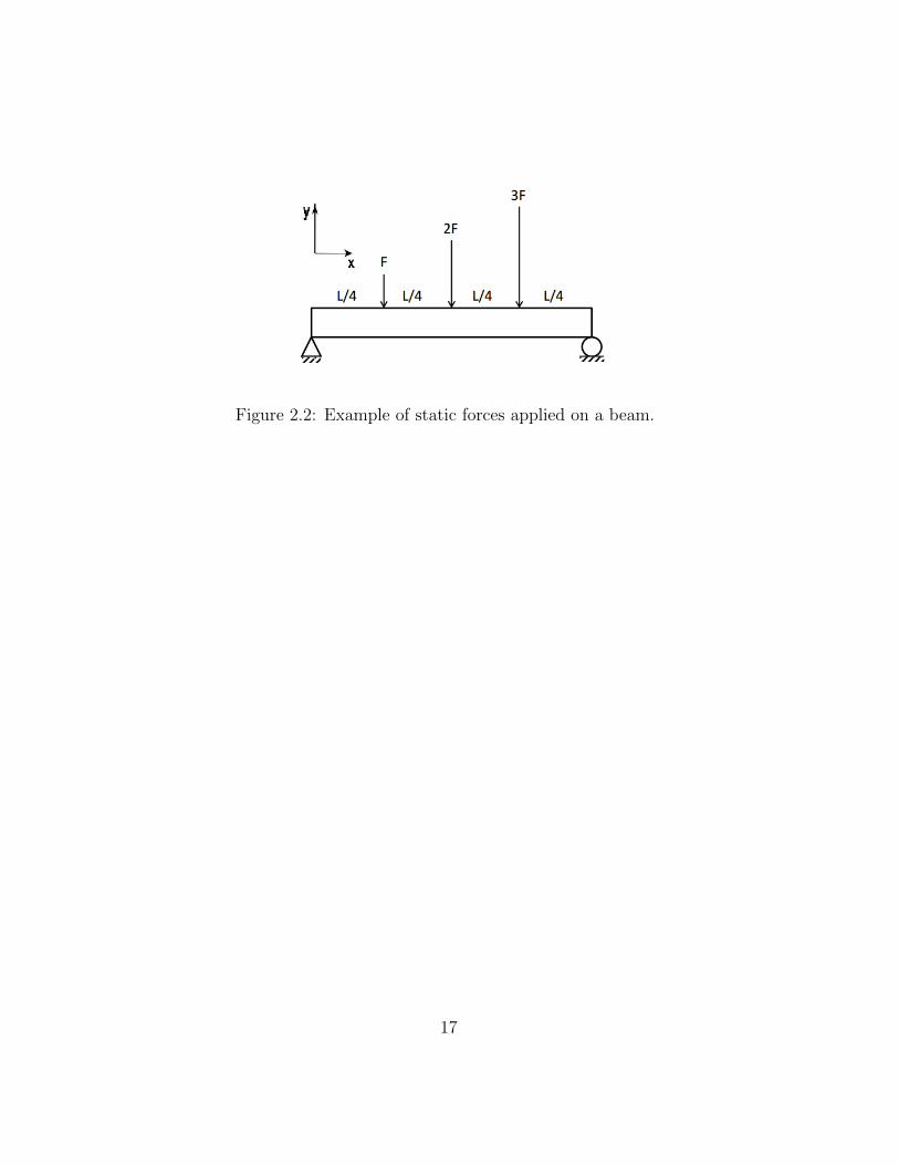
Figure 2.2: Example of static forces applied on a beam.

17

Chapter 3

Method

In this chapter the approach and method of this thesis are presented. Itconsists of the generation of concepts with CAD-drawings and parametersfor the calculation of measurement uncertainty.

3.1 Generating Concepts

The concept generating phase was not a regular concept generation withmatrices and brainstorming-drawings, since BorgWarner already knew howthey wanted the concepts to look like. The concept generating phase insteadconsisted of putting different gearboxes together with multiple adapters andmountings. To be able to use BorgWarner’s existing products (e.g. adapters,shafts etc.) and get better prices, the concepts focused on existing suppliersof gearboxes and motors.

3.1.1 Specifications

The process of generating concepts most important step is where the applic-ation requirements is set. The specification was set in the beginning of thesecond week at BorgWarner, which made the continued work easier and bet-ter organized. The specifications were set together with the supervisor andone of his colleagues at the department. The most vital parts of the require-ment specifications are presented in table 3.1 and the rest of the parameterscan be seen in Appendix Requirement Specifications.

18

Table 3.1: The most vital parameters from the Appendix Requirement Spe-cifications.

Mobile Lifting PointsMeasure up to ±5 kNm (Rev ±3 kNm) Measure in both directionsStatic measuring points Calibrated T12 as reference

3.1.2 Torque Transducer

The torque transducer that will be both the reference and the measurand isthe HBM T12 [21]. This torque transducer is, with its high accuracy overa large range of torque, perfect for this application. The T12 comes witheight different maximal nominal torques, from 100 Nm to 10 kNm. In thisrig concept the HBM T12 3 kNm is used. It is with data from the T12’s datasheet that the measurement uncertainty will be calculated.

3.1.3 Gearbox

The two existing gear and gearbox suppliers for BorgWarner are NORD andSiemens, which made the selection of gearbox suppliers very easy. Both sup-pliers are well known in the industry with high durability and good quality.Industry gearboxes comes in many forms and types, the gearboxes evaluatedin this thesis are parallel shaft gearboxes and helical gearboxes. These twotypes are the least space consuming with high strength.

3.1.4 Motor

The motor for all concepts is a servo motor from Kollmorgen. This motoris used because BorgWarner already has the knowledge, software and equip-ment to run and observe motors from Kollmorgen. The selection of a servomotor from Kollmorgen is based on the money saved in components andespecially the amount of time saved by avoiding to learn a new software.

3.1.5 Prop shaft

The prop shaft is a standard prop shaft used in other applications at BorgWarner.The selected prop shaft is a hollow shaft with flexible joints. Other propshafts could be mounted on to the system, but then additional adapters

19

would be needed. Prop- and drive shafts that have strain gauge attachedonto them to measure torque can also be calibrated in the rig, and requiredifferent adapters as well as a mounting for fixation.

3.1.6 Adapters

Multiple adapters are needed to be able to fit everything together. Thereare adapters from the gearbox output axle to the reference transducer, fromthe transducer to a torque limiter, and all the way to the transducer to becalibrated. A large amount of adapters are designed to work together withBorgWarners existing products.

3.1.7 Mountings

Mountings for the gearboxes are needed to get the rigs to be stable and atthe right place. If the mountings would be unstable or even worse be failingto keep the rigs in position the consequences would be devastating. Due tothe flexible joints on the shafts a small instability in the mounting would notdestroy the transducer but the calibration would be worthless. As mentionedin the previous section, a mounting for prop- and drive shafts that has sensorattached onto them is also needed. This mounting needs to have differentsizes and patterns in order to fit all the different prop- and drive shafts. Themountings for the gearboxes needs to center the output axle at a height of 240mm from the floor, see appendix Existing Rigs. The mounting itself needs tobe bolted to the floor, which consists of steel plates on top of a frame made outof beams. The steel plates are 1200 mm times 1200 mm and have a patternof holes drilled into them. The holes are drilled with a distance of 100 mmbetween them, see appendix Existing Rigs. To adjust the mounting positionof the calibration rig the mountings to the floor have elongated circular holesinstead of circular with a fixed diameter. The elongated holes are in theY-direction because the existing motor and transducer could move in the X-direction. The holes are fitted with a distance of 100 mm respectively 300 mmsee figure 3.1. On one side the mounting for the gearbox is combined witha mounting for the transducer. The transducers mounting is divided intotwo parts. One part is fixed the floor together with the gearbox mountingand the other part is free to move in the Y-direction. The second part haselliptical holes for the transducer mounting to easily adjust the position ofthe transducer in both X- and Z-direction, see figure 3.2.

20

(a) Concept A

(b) Concept B

Figure 3.1: Distance between mounting holes in to the floor.

21

Figure 3.2: Mounting for torque transducer with possibilities to adjust theposition in every direction.

3.1.8 Electronic encapsulation

Two boxes (encapsulation) for the servo motor drive and the measurementelectronics needs to be fitted to the application as well. These boxes needto be placed where they are not in the way for something else like boltsor screws but also are close to the transducer and the servo motor to savecabling. The electronic boxes needs extra mountings but thanks to the lowweight at the encapsulation the mountings could be kept simple.

3.1.9 Torque Limiter

A torque limiter is a device that lets torque be transferred until the torquegets too high. The value that can be transferred is selected with breakpins with different strength. The maximum torque transferred through this

22

limiter is 3100 Nm. The torque limiter is made by HOWDON Power Trans-mission Ltd in Great Britain. The torque limiter has four break pins and hasa hole pattern different from the transducer. The limiter is shown in figure3.3.

Figure 3.3: Torque limiter used in the application for safety [22].

3.2 Software

Different software were used at the company and the university to make theCAD-models, which caused a minor issue with the selection of software. Tosave time it was decided to continue with the already familiar program thatis used at the university which is the Siemens NX 11 [23]. With this programall the CAD-models, a simple FEM-analysis, and simulation on the gearboxmounting were made. The software to calculate the total measurement un-certainty is Microsoft Excel, which made the calculation easy to survey andadjust.

23

3.3 Calculation of Measurement Uncertainty

The method to calculate the measurement uncertainty of the transducer isdescribed here. The procedure captures the calculation of the systems para-sitic loads, total measurement uncertainty and expanded total measurementuncertainty.

3.3.1 Parameters of the application

The parameters needed to be evaluated in a calculation of measurementuncertainty are stated in the data sheet of the Torque Transducer T12,[24].In this application a T12 with a maximal measurable capacity of 3 kNm isused. Parameters from the data sheet and the application are summarized intable 3.2. In the table a column “Distribution Factor” is shown, these valuescome from the previous chapter Theory and the equation 2.7. The valuesunder “Process” are from the specification earlier mentioned. Under thecategory “Design of Arrangement” are a parameter “Total Parasitic Loads”stated, these loads needs to be calculated.

24

Table 3.2: Measurement Uncertainty Parameters from the data sheet andapplication (Fieldbuses/ Frequency output).

Distribution FactorParameter Unit Related to Rectangle Normal Value (±)

Transducer

Sensitivity Tolerance % Maximum Torque 0.58 0.05Relative standarddeviation of repeatability

% ∆ Torque 1 0.01

Non-linearity includinghysteresis

% Full Range 0.58 0.02

Temperature effectper 10 K in thenominal temperaturerange on the zero signal,related to the nominalsensitivity (TK0)

% Full Range 0.58 0.02

Temperature effectper 10 K in the nominaltemperature rangeon the output signal,related to theactual value of thesignal span (TKC)

% Maximum Torque 0.58 0.03

Design ofSystem

Total Parasitic loads % Full Range 0.58

Process

Maximal Torque ofthe application

Nm ±3000

Full Range of Torque Nm 3000Maximal Temperatureof the Transducer

◦C 25

Minimal Temperatureof the Transducer

◦C 21

3.3.2 Method to calculate the measurement uncertainty

To obtain a greater knowledge regarding how to perform a correct calculationof measurement uncertainty, sensor and transducer manufacturer HBM wascontacted. HBM has a great reputation in the measurement industry, withmany sensors and transducers measuring force, strain and torque. They oftenhave webinars and have many examples to perform calculations of uncertaintyof measurement systems with their sensors and transducers. HBM contrib-uted with different examples of calculations and descriptions of parametersand important steps in the procedure. With the help from the examples andthe supervisors at BorgWarner ensured a correct method was implemented

25

for the calculation of measurement uncertainty.

26

27

Chapter 4

Results

In this chapter the results are presented. It is divided into one section forthe results of the Measurement Uncertainty and one section for the conceptsand the cost analysis.

4.1 Measurement Uncertainty of the Torque

Transducer

The calculation matrix for the total measurement uncertainty of the torquetransducer can be seen in table 4.1. In this table every value contributingto the total measurement uncertainty is displayed. At the top of the tablethe Parameters of the application are displayed, these values are determinedtogether with a group of experts from BorgWarner. The parasitic loads weredetermined through the description above, but after consultation they wereconsidered to low so safety factors were included. As seen in table 3.2 thedistribution is rectangular, which means that it is considered to be this bador better. In other words, the calculated value of measurement uncertaintyis the worst case scenario. The result with a measured torque of 3000 Nmand a uncertainty of ±2.257 Nm at 95.45% is really good. The variation isunder 0.1%, which is considered good depending on the conditions for thetransducer. The work range of the transducer is from +100% to −100%which makes the small variation even more noticeable.

28

Table 4.1: Calculation of worst case scenario Measurement Uncertainty of aHBM T12 Torque Transducer in laboratory environment.

Parameters of theapplication

Unit

Max. Torque of theapplication = Max. Torque

[Nm] 3000

Min. Torque of theapplication = Min. Torque

[Nm] -3000

∆ Torque [Nm] 6000Max. Temp. of thetransducer = Max. Temp

[◦C] 26

Min. Temp. of thetransducer = Min. Temp

[◦C] 20

∆ Temp [◦C] 6Parasitic Loads Safety FactorAxial Force [kN] 2 0 0Lateral Force [kN] 2 0,135 0,27Bending Moment [Nm] 2 11 22

Parameters of the datasheet (Fieldbuses/Frequency output)

T12 - 3kNDistributionFactor

Distribution MU [Nm]

Full Range [Nm] 3000Sensitivity tolerance(% of max. Torque)

[%] 0,05 0,58 Rectangular 0,87

Non-Linearity deviationincluding Hysteresis(% of full range)

[%] 0,02 0,58 Rectangular 0,348

Temperature deviationon the zero point per 10Kdeviation from 23◦C(% of full range)

[%] 0,02 0,58 Rectangular 0,1044

Temperature deviation onthe sensitivity per 10Kdeviation from 23◦C(% of Max Torque)

[%] 0,03 0,58 Rectangular 0,1566

Relative standarddeviation of repeatability(% of max. Torque)

[%] 0,01 1 Normal 0,6

PercentageAxial Limit Force [kN] 42 0Lateral Limit Force [kN] 10 2,7Bending Limit Moment [Nm] 600 3,666666667Impact of ParasiticLoads (% of full range)

[%] 0,3

Total Parasitic Loads [%] 0,58 Rectangular 6,366666667 0,33234Factor

Total MeasurementUncertainty

[Nm] ± 1,128462193

Extended MeasurementUncertainty (90%)

[Nm] 1,645 ± 1,856320307

Extended MeasurementUncertainty (95,45%)

[Nm] 2 ± 2,256924385

Extended MeasurementUncertainty (99%)

[Nm] 2,576 ± 2,906918608

29

4.2 The Concepts (A & B)

The proposed concepts made are very similar to each other due to the sameimplications and products surrounding them. A few things are differentmainly: the height and width of the mounting holes on the sides of thegearbox. The displacement and the stress were simulated through a simpleFEM-analysis. The simulations make the displacement look bigger than itis in real life. The simulated loads could never appear in a real life situationbecause in the simulations all loads were applied to one single mounting andin real life there are at least three mountings bearing the load. The loadsapplied to this mounting is the load from the gearbox weight and the torqueproduced by the servo motor inside the gearbox divided into forces that wantto rotate the mounting. A discussion around the results follows in the chapterDiscussion. The forces applied on the mountings during the FEM-analysisare at the same amplitude for both mountings even if one gearbox is lighter.The forces applied during the FEM-analysis are the weight of the gearboxand the servomotor times the standard acceleration due to gravity appliedinside the bolt holes. To easily apply the torque in the analysis, it is dividedinto pressure and tensile forces times the distance from the center of thegearbox to the mounting. The total torque produced in the rig is 3 kNmbut it is divided on to multiple mountings. To have high safety factor in theFEM-analysis the simulated torque on one mounting is 3 kNm. The resultsof the FEM-simulation is presented later in this section.

Gearbox type

Earlier in this thesis different types of gearboxes were evaluated and the typethat has the most advantages is the parallel shaft gearbox. It has a highermaximum torque and a better range of ratios. One advantage that is shownlater is the high placement of the servo motor. This made the placement ofthe encapsulation easier, this can be seen in appendix Concepts.

4.2.1 Concept A - Gearbox from NORD

The final concept for concept A is shown in figure 4.1 and more pictures canbe found in appendix Concepts.

30

Figure 4.1: Concept A from side view.

Displacement

The displacement of the mounting is 0.140 mm, see figure 4.2

Stress - von Mises

The stress appeared in the mounting is 102.72 MPa, see figure 4.3, which isconsidered good and has a safety factor of around 4.

4.2.2 Concept B - Gearbox from Siemens

The final concept for concept B is shown in figure 4.4 and more pictures canbe found in appendix Concepts.

Displacement

The displacement of the mounting is 0.854 mm, see figure 4.5.

31

Figure 4.2: Simulated displacements on mountings for NORD concept.

Figure 4.3: Simulated stress (von Mises) on mountings for NORD concept.

32

Figure 4.4: Concept B from side view.

Figure 4.5: Simulated displacements on mountings for Siemens concept.

33

Stress - von Mises

The stress appeared in the mounting is 275.07 MPa, see figure 4.3, which isconsidered a bit high and has a safety factor of around 1.5.

Figure 4.6: Simulated stress (von Mises) on mountings for Siemens concept.

Dimensions

Dimensions of the different concepts could be found in Table 4.2.

Table 4.2: Dimensions of the concepts. All measuremens are in millimetersand kilograms.

Dimension Concept A Concept BHeight 650 720Length 1 070 1 090Width 790 830Weight 380 (225) 330 (187)

4.2.3 Shaft fixation

One fixation for prop- and drive shaft has been designed. The idea was to beable to mount every shaft on the fixation without adapters but unfortunatelythis was not possible. It was not possible because of the small change in

34

diameter of the different shafts. This made the design of the fixation simplewith adapters for every shaft. An example of a shaft mounted to the fixationis shown in figure 4.7. More pictures of the fixation and the adapters can befound in appendix Concepts.

Figure 4.7: Example of a shaft mounted to the fixation and adapters forother shafts.

35

4.2.4 Safety

One important aspect in the Requirement Specifications is the safety regard-ing high torque applications. With the rigs high static torque loads it isimportant to know that all the tensions in the shaft have been canceled tobe able to go into the room and work. Within the servo motor control pro-gram it could be seen if the motor have been rotating backwards to the pointwhere tension was present. A visual safety feature is also implemented forthe operator. The visual safety feature is a very simple line drawn with amarker of a different colour than the shaft. This line is drawn straight and ifthe line is curved the operator knows that some high residual torque is stillapplied to the shaft and thus should not work on the rig yet.

4.2.5 Cost analysis

Table 4.3 shows the cost estimates for the concepts. The prices for adaptersand mountings are the most uncertain estimate due to the fact that all ad-apters and mountings is going to be specially made for this rig. This makes ithard to get an exact offer without production ready drawings. If the price isassumed to be a relation between material and complexity than concept B’smountings should be cheaper because of the smaller volume. The exact priceof the adapters and mountings is not evaluated due to that there are not anyproduction ready drawings. To get the exact price from the manufacturerthere is a need of drawings and then they need time to estimate the correctprice. Unfortunately the time is not on this thesis side, and therefor is notany time available to wait for a price estimate. The price is based on earlierprices on adapters from the same manufacturer.

36

Table 4.3: Cost analysis of concepts. All prices are in SEK ex. VAT.

Product Concept A Concept BGearbox 28 587 25 501Servo motor 21 673 21 673Torque limiter 4 369 4 369Torque transducer 113 820 113 820Transducer certificate 9 963 9 963Servo motor cabling 2 226 2 226Servo motor drive 10 862 10 862Adapters 6 000 6 000Mounting 5 000 5 000Encapsulation 5 970 5 970Total 208 470 205 384

37

Chapter 5

Discussion

Concepts

The two concepts are very similar to each other. That is because BorgWarneralready had an idea of how the concept would look like. The concepts aremade to be as compact and have as high mobility as possible. This is why theconcepts have the same type of gearbox, it could have been two different typesbut then it would be easy to say which concept is better in the mobility pointof view. Different types of motors could also have been evaluated but, likestated earlier, it would have created more work during the implementationand testing phase. This is why the same servo motor from an already knownmanufacturer is chosen.

Measurement Uncertainty

The result of the calculated measurement uncertainty is considered reallygood for the torque calibration rig under controlled circumstances. Con-trolled circumstances meaning under the correct temperature and humidity.The correct temperature is between 20◦C to 26◦C which is the normal tem-perature indoors. Normal humidity indoors is somewhere between 25 to 55 %.The measurement uncertainty is like stated earlier the worst case measure-ment uncertainty, which means that the calculated value could not be higher.It is because of the rectangular distribution that are used to calculates themeasurement uncertainty from the highest and lowest values observed in e.g.,

38

the data sheet. The rectangular distributions are reasonable due to insuffi-cient knowledge about the input quantity. When measurements have beenmade and evaluated better distributions could be used. Distributions thatmight be better are triangle- or normal distribution. These distributions arebetter than rectangular distributions if the measured values is in the middleof the variability interval. Rectangular- or U-shaped distributions are pre-ferred if the measured values are more likely to be close to the limits. Evenmore noticeable is when lower torque is measured, then the uncertainty de-creases because of when determining the measurement uncertainty there aretwo parameters depending on what is measured. The parameters are the“Non-Linearity deviation including Hysteresis” and “Temperature deviationon the zero point per 10K deviation from 23◦C”, which both depends on the“Full Range” of the measurement. Another improvement of the measurementuncertainty is to only measure during 23◦C, because that is the transducer’sreference temperature. Then both “Temperature deviation on the zero pointper 10K deviation from 23◦C” and “Temperature deviation on the sensitivityper 10K deviation from 23◦C” would be decreasing. All these values can befound in Table 4.1 in Chapter Results.

39

40

Chapter 6

Conclusion

The conclusion is that this is an important area for BorgWarner to ensurecorrect measurements, both internally within BorgWarner and externally outto customers. Measurement uncertainty is an area where more work needsto be done at BorgWarner to get better knowledge in the subject. The resultof the calculated measurement uncertainty for the calibrated transducer isgood. The concept models are designed and awaits decision from higherinstances to go forward with one of the concepts.

41

42

Chapter 7

Further work

Due to this thesis only being a concept study of a new torque calibration rig,much work is still needed to implement torque calibration. In this project,many things are still needed to convert the process into reality. The firststep into making this project reality is to take a decision if torque calibrationof the sensors is needed and if it would be more expensive than today. Aproper cost investigation for today’s calibration has to be done. This invest-igation is needed to find out whether there is money to be saved or not. Ifthe decision is to go on and build a torque calibration rig, there is still muchwork to do. All CAD-models must be checked for errors, and to make surethat the models runs smooth. Drawings of mountings and adapters has to bemade and sent to the manufacturer. Together with adapters and mountingsbeing checked, all the other equipment needs to be ordered from the suppli-ers. After everything is ordered and has arrived the installation begins. Allparts are mounted together and all the electronics are wired and encapsu-lated. Then the implementation and testing of the rig begins. Calibrationinstructions and report templates are needed to be done in order to simplifythe calibration of the torque transducers in the existing rigs.

43

44

Appendix A

Requirement Specifications

45

Kravspec Mobil, lyftöglor

Mäta upp till 5kNm

Kalibrera kardan, extra fixtur för att låsa kardan

Använda T12 som referens

Fast höjd-distans under (lägsta höjden i tiltriggen) (240 mm)

Undersöka momentalstrare

Motortyp (ex servo, asynkron, hydraulisk)

Moment i båda riktningar

Statiska mätpunkter

Koncept för axel och axelkopplingar

Pris-estimat,

Figure A.1: Mind map to get an easier overview of the torque calibration rigrequirements.

47

Appendix B

Existing Rigs

Drawing of height in existing rigs.

48

Figure B.1: Drawing of steel plates in rig room with holes.

50

Figure B.2: Steel plate in rig room without dimensions.

51

Appendix C

Concepts

C.1 Concept A

Figure C.1: View from transducer and shaft side.

52

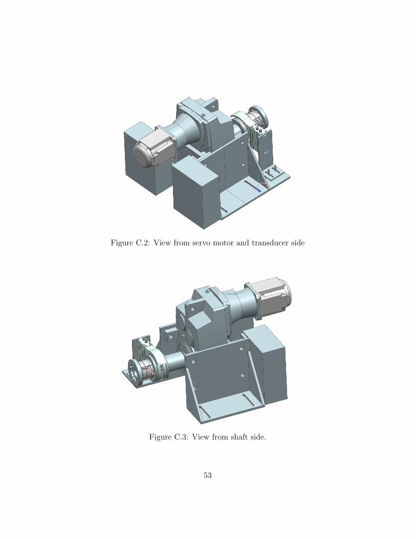
Figure C.2: View from servo motor and transducer side

Figure C.3: View from shaft side.

53

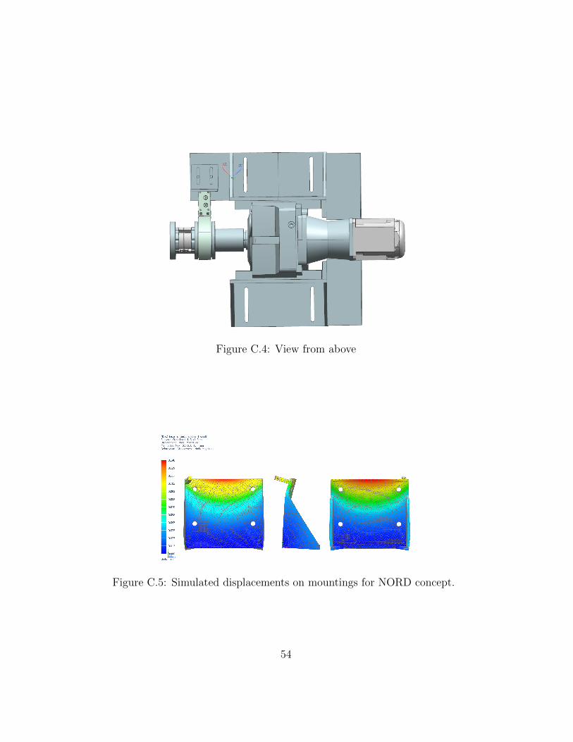
Figure C.4: View from above

Figure C.5: Simulated displacements on mountings for NORD concept.

54

Figure C.6: Simulated stress (von Mises) on mountings for NORD concept.

C.2 Concept B

55

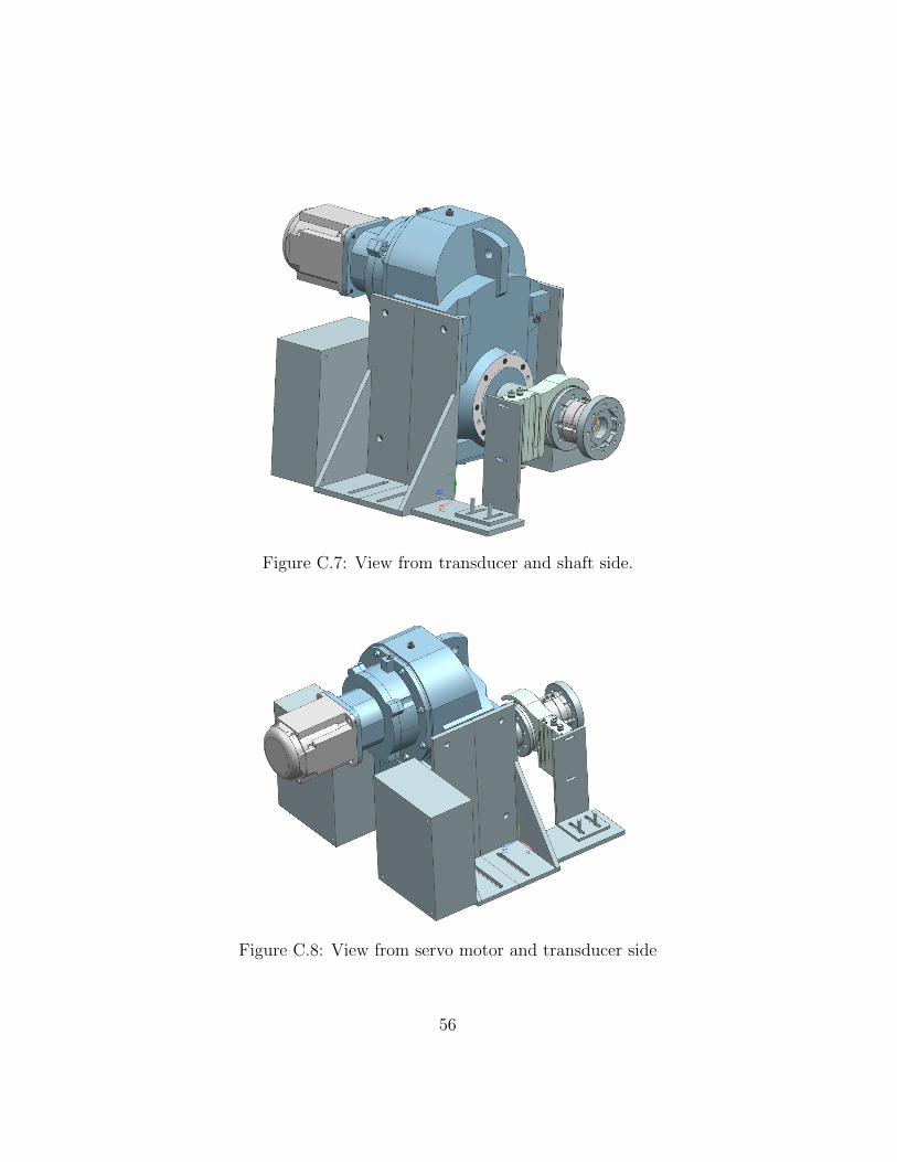
Figure C.7: View from transducer and shaft side.

Figure C.8: View from servo motor and transducer side

56

Figure C.9: View from shaft side.

Figure C.10: View from above

57

Figure C.11: Simulated displacements on mountings for concept B.

Figure C.12: Simulated stress (von Mises) on mountings for concept B.

58

C.3 Adapters

Figure C.13: Fixation for shafts, different adapters and an example shaft.

59

Figure C.14: Shaft fixation viewed from above.

60

C.4 Adapters

Figure C.15: Adapter from 108 mm to 68 mm.

61

Figure C.16: Adapter from 108 mm to 74 mm.

62

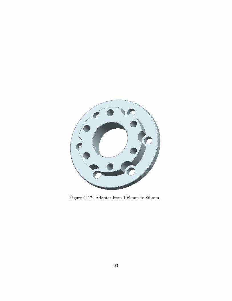
Figure C.17: Adapter from 108 mm to 86 mm.

63

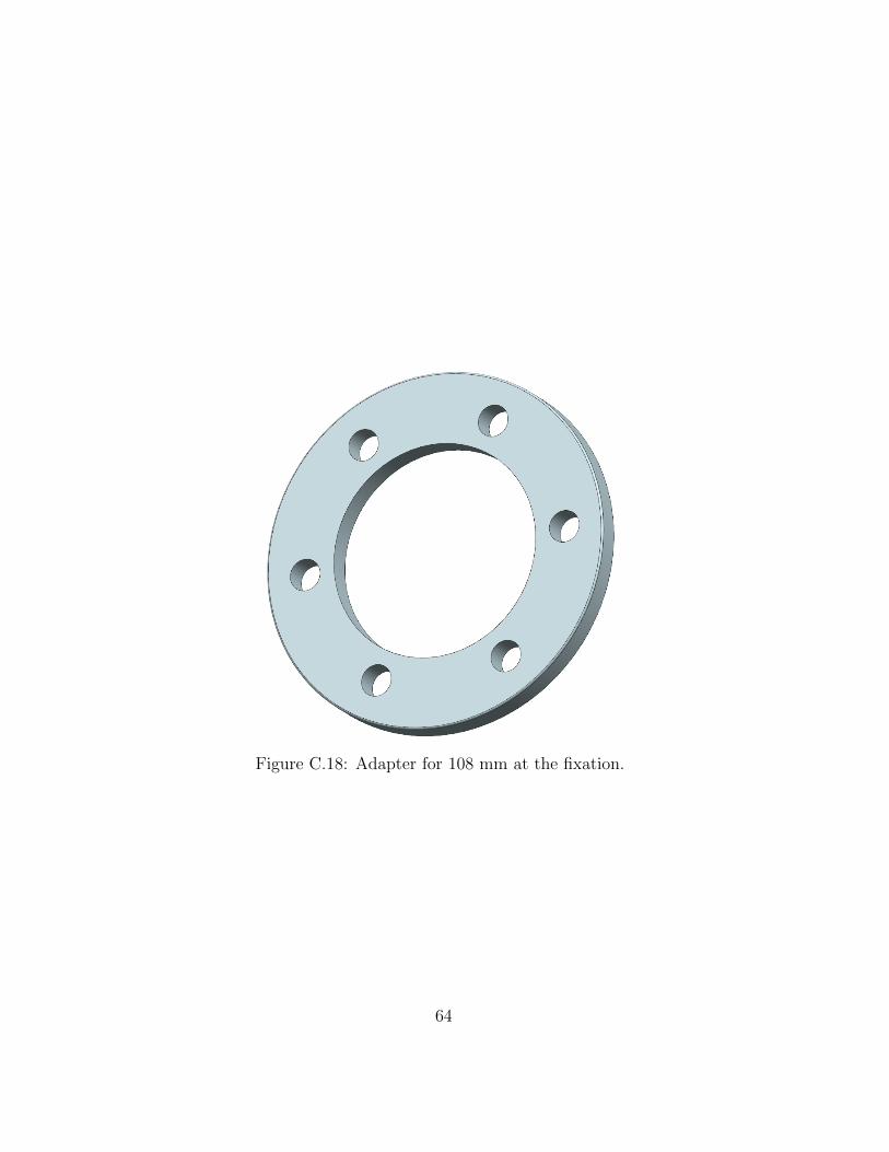
Figure C.18: Adapter for 108 mm at the fixation.

64

Figure C.19: Adapter between HOWDON and T12 (130 mm hole picture),with recessed bolt holes.

65

Figure C.20: Adapter between T12 (130 mm) and HOWDON, with recessedbolt holes.

66

Appendix D

Project Planning

D.1 Project plan

67

Momentkalibrering

Inledning/Bakgrund

Idag sitter momentgivarna inmonterade i riggar och för att momentgivarna skall kalibreras måste

givarna monteras ur riggen och skickas till extern firma. Detta vill BorgWarner slippa i framtiden.

BorgWarner vill istället göra kalibreringen in-house genom att bygga en momentkalibreringsrigg så

att momentgivarna kan sitta kvar i riggen samtidigt som de kan kalibreras. Kalibreringen måste göras

mot en annan momentgivare som är spårbart kalibrerad gentemot en nationell normal. BorgWarner

måste kunna visa att deras givare är kalibrerade gentemot en nationell normal på deras verifierande

prov. Efter kalibrering görs eventuellt en justering utav mätdonet.

Syfte

Ta fram ett koncept för en momentkalibreringsrigg som säkerställer att momentgivarna visar rätt värde jämfört med nationell normal. Alla mätningar som är gjorda sedan senaste kalibreringstillfället blir ogiltiga om en givare ej klarar kalibreringen för då kan man inte veta säkert att den har visat rätt (och när den slutat visa rätt). Därför vill BorgWarner ha möjlighet att på ett relativt simpelt vis kalibrera sina givare ofta och så

billigt som möjligt då det är dyrt att demontera givare och skicka iväg dessa till extern kalibrerings

firma.

Frågeställning

Är det möjligt på enkelt och smidigt sätt kalibrera momentgivare utan att plocka ut dessa ur

riggen utan att tumma på noggrannhet eller repeterbarhet?

Metod

Utifrån kravspecifikationen hitta olika koncept på hur kalibrering kan utföras. Dessa koncept skall

sedan diskuteras med ansvariga på BorgWarner och det slutgiltiga konceptet skall CAD:as och

kostnadsberäknas. I det olika koncepten skall drivmotor, axel och axelkopplingar definieras.

Tidplan

Se bilaga 1 och 2 för Fasschema och Gantt-schema.

D.2 Risk Analysis

69

Riskanalys

Risk

Sannolikhet

(1-5)

Konsekvens

(1-5) Totalt Åtgärd

Sjukdom 1 4 4 Arbeta hemma

Utökad tidsåtgång 3 4 12 Längre arbetsdagar och effektivare arbete

Datorproblem 2 5 10

Börja om, det borde gå fort då allt redan

är gjort en gång

Informationssökning ger

lite information 2 3 6

Utöka sökning, ring andra företag som

håller på med momentkalibrering

Strömavbrott (Detta

hände) 1 4 4

Arbeta hemma, alternativt hitta någon

annastans på företaget

D.3 Gantt

71

Bibliography

[1] Definition and history of torque. https://en.wikipedia.org/wiki/

Torque. [Online; accessed 30 March, 2017].

[2] Arcimedes. https://en.wikipedia.org/wiki/Archimedes. [Online;accessed 30 March, 2017].

[3] Definition of torque. https://www.physics.uoguelph.ca/tutorials/torque/Q.torque.intro.html. [Online; accessed 30 March, 2017].

[4] Borgwarner history. https://www.borgwarner.com/en/company/

history. [Online; accessed 29 March, 2017].

[5] Borgwarner history. https://en.wikipedia.org/wiki/BorgWarner.[Online; accessed 29 March, 2017].

[6] Borgwarner engine group products. https://www2.borgwarner.com/

en/Products/default.aspx. [Online; accessed 29 March, 2017].

[7] Borgwarner drivetrain group products. https://www2.borgwarner.

com/en/Drivetrain/Pages/Products.aspx? [Online; accessed 29March, 2017].

[8] Products from borgwarner drivetrain group. https://

www2.borgwarner.com/en/powerdrive/products/Literature/

Drivetrain%20Brochure.pdf. [Online; accessed 7 April, 2017].

[9] BorgWarner. PowerDrive Systems, Torque Management and VehicleDynamics. BorgWarner PowerDrive Systems Germany, 2011.

[10] Haldex genv awd coupling. http://www.nyteknik.se/fordon/

borg-warner-fyrhjulsdrift-ar-har-for-att-stanna-6394639.[Online; accessed 30 May, 2017].

72

[11] Ulf Herlin & John Barlage. GenV AWD Coupling. BorgWarnerTorqTransfer Systems, 2014.

[12] Genv awd coupling. https://www2.borgwarner.com/en/powerdrive/products/Pages/GenerationV.aspx. [Online; accessed 3 April, 2017].

[13] Bjorn Hedmark. Pre-study of rig testing implementation from real worlddriving. Master’s thesis, Lulea University of Technology, 2016.

[14] History of length measurement. http://www.npl.co.uk/upload/pdf/

history-of-length-meas-poster.pdf. [Online; accessed 5 April,2017].

[15] History of bureau international des poids et mesures, short bipm. http://www.bipm.org/en/measurement-units/history-si/. [Online; ac-cessed 5 April, 2017].

[16] Definition of meter from bipm. http://www.bipm.org/en/

measurement-units/base-units.html. [Online; accessed 5 April,2017].

[17] Stephanie Bell. A Beginner’s Guide to Uncertainty of Measurement.Crown & National Physical Laboratory, Aug 1999. [ISSN: 1368-6550].

[18] JCGM Joint Committee for Guides in Metrology. International vocab-ulary of metrology — Basic and general concepts and associated terms(VIM). BIPM, 2008.

[19] EA Laboratory Committee. Evaluation of the Uncertainty of Measure-ment In Calibration. European Accreditation, second swedish editionedition, September 2013.

[20] Parasitic loads described by hbm. https://www.hbm.com/en/0803/

tips-and-tricks-torque-parasitic-loads/. [Online; accessed 21April, 2017].

[21] Description of hbm t12. https://www.hbm.com/se/2377/

t12-ultra-high-precision-digital-torque-transducer/. [Online;accessed 25 April, 2017].

[22] Picture of torque limiter. https://hiveminer.com/User/

howdonpower/Interesting. [Online; accessed 11 May, 2017].

73

[23] Siemens nx 11. https://www.plm.automation.siemens.com/en/

products/nx/11/. [Online; accessed 15 May, 2017].

[24] HBM Hottinger Baldwind Messtechnik GmbH. T12 Digital TorqueTransducer Data Sheet. HBM, 2010.

74