Variational Methods for Inference and Estimation inGraphical ModelsbyTommi S. Jaakkola1Department of Brain and Cognitive SciencesMassachusetts Institute of TechnologyCambridge, MA 02139c Massachusetts Institute of Technology 1997AbstractGraphical models enhance the representational power of probability models throughqualitative characterization of their properties. This also leads to greater e�ciencyin terms of the computational algorithms that empower such representations. Theincreasing complexity of these models, however, quickly renders exact probabilisticcalculations infeasible. We propose a principled framework for approximating graph-ical models based on variational methods.We develop variational techniques from the perspective that uni�es and expandstheir applicability to graphical models. These methods allow the (recursive) compu-tation of upper and lower bounds on the quantities of interest. Such bounds yieldconsiderably more information than mere approximations and provide an inherenterror metric for tailoring the approximations individually to the cases considered.These desirable properties, concomitant to the variational methods, are unlikely toarise as a result of other deterministic or stochastic approximations.The thesis consists of the development of this variational methodology for prob-abilistic inference, Bayesian estimation, and towards e�cient diagnostic reasoning inthe domain of internal medicine.Thesis Supervisor: Michael I. JordanTitle: Professor1E-mail: tommi@psyche.mit.edu.

Contents1 Introduction 41.1 Convex duality and variational bounds : : : : : : : : : : : : : : : : : 81.2 Overview : : : : : : : : : : : : : : : : : : : : : : : : : : : : : : : : : : 101.A Bounds and induced metrics : : : : : : : : : : : : : : : : : : : : : : : 132 Upper and lower bounds 162.1 Introduction : : : : : : : : : : : : : : : : : : : : : : : : : : : : : : : : 162.2 Log-concave models : : : : : : : : : : : : : : : : : : : : : : : : : : : : 172.2.1 Upper bound for log-concave networks : : : : : : : : : : : : : 182.2.2 Generic lower bound for log-concave networks : : : : : : : : : 212.3 Sigmoid belief networks : : : : : : : : : : : : : : : : : : : : : : : : : : 232.3.1 Upper bound for sigmoid network : : : : : : : : : : : : : : : : 232.3.2 Generic lower bound for sigmoid network : : : : : : : : : : : : 242.3.3 Numerical experiments for sigmoid network : : : : : : : : : : 242.4 Noisy-OR network : : : : : : : : : : : : : : : : : : : : : : : : : : : : 262.4.1 Upper bound for noisy-OR network : : : : : : : : : : : : : : : 272.4.2 Generic lower bound for noisy-OR network : : : : : : : : : : : 272.4.3 Numerical experiments for noisy-OR network : : : : : : : : : 282.5 Discussion and future work : : : : : : : : : : : : : : : : : : : : : : : : 292.A Convexity : : : : : : : : : : : : : : : : : : : : : : : : : : : : : : : : : 312.B Sigmoid transformation : : : : : : : : : : : : : : : : : : : : : : : : : : 322.C Noisy-OR transformation : : : : : : : : : : : : : : : : : : : : : : : : : 332.D Noisy-OR expansion : : : : : : : : : : : : : : : : : : : : : : : : : : : 342.E Quadratic bound : : : : : : : : : : : : : : : : : : : : : : : : : : : : : 353 Recursive algorithms 373.1 Introduction : : : : : : : : : : : : : : : : : : : : : : : : : : : : : : : : 373.2 Recursive formalism : : : : : : : : : : : : : : : : : : : : : : : : : : : 383.2.1 Probability models : : : : : : : : : : : : : : : : : : : : : : : : 383.2.2 The formalism : : : : : : : : : : : : : : : : : : : : : : : : : : : 393.2.3 Transformation : : : : : : : : : : : : : : : : : : : : : : : : : : 393.2.4 Recursive marginalization : : : : : : : : : : : : : : : : : : : : 413.2.5 Exact computation : : : : : : : : : : : : : : : : : : : : : : : : 433.3 Examples : : : : : : : : : : : : : : : : : : : : : : : : : : : : : : : : : 443.3.1 Boltzmann machines : : : : : : : : : : : : : : : : : : : : : : : 442

3.3.2 Sigmoid belief networks : : : : : : : : : : : : : : : : : : : : : 483.3.3 Chain graphs : : : : : : : : : : : : : : : : : : : : : : : : : : : 493.4 Discussion : : : : : : : : : : : : : : : : : : : : : : : : : : : : : : : : : 493.A Lower bound : : : : : : : : : : : : : : : : : : : : : : : : : : : : : : : 513.B Upper bound : : : : : : : : : : : : : : : : : : : : : : : : : : : : : : : 514 Bayesian parameter estimation 534.1 Introduction : : : : : : : : : : : : : : : : : : : : : : : : : : : : : : : : 534.2 Bayesian logistic regression : : : : : : : : : : : : : : : : : : : : : : : : 544.3 Accuracy of the variational method : : : : : : : : : : : : : : : : : : : 554.4 Comparison to other methods : : : : : : : : : : : : : : : : : : : : : : 564.5 Extension to belief networks : : : : : : : : : : : : : : : : : : : : : : : 584.5.1 Incomplete cases : : : : : : : : : : : : : : : : : : : : : : : : : 584.6 The dual problem : : : : : : : : : : : : : : : : : : : : : : : : : : : : : 614.7 Technical note: ML estimation : : : : : : : : : : : : : : : : : : : : : : 634.8 Discussion : : : : : : : : : : : : : : : : : : : : : : : : : : : : : : : : : 634.A Optimization of the variational parameters : : : : : : : : : : : : : : : 644.B Parameter posteriors through mean �eld : : : : : : : : : : : : : : : : 654.B.1 Mean �eld : : : : : : : : : : : : : : : : : : : : : : : : : : : : : 654.B.2 Parameter posteriors : : : : : : : : : : : : : : : : : : : : : : : 674.B.3 Optimization of the variational parameters : : : : : : : : : : : 685 Variational methods in medical diagnosis 715.1 Introduction : : : : : : : : : : : : : : : : : : : : : : : : : : : : : : : : 715.2 The QMR-DT belief network : : : : : : : : : : : : : : : : : : : : : : 725.3 Inference : : : : : : : : : : : : : : : : : : : : : : : : : : : : : : : : : : 735.4 Variational methods : : : : : : : : : : : : : : : : : : : : : : : : : : : 755.4.1 A brief introduction : : : : : : : : : : : : : : : : : : : : : : : 755.4.2 Variational methods for QMR : : : : : : : : : : : : : : : : : : 755.5 Towards rigorous posterior bounds : : : : : : : : : : : : : : : : : : : 785.6 Results : : : : : : : : : : : : : : : : : : : : : : : : : : : : : : : : : : : 805.6.1 Comparison to exact posterior marginals : : : : : : : : : : : : 805.6.2 Comparison to Gibbs' sampling estimates : : : : : : : : : : : 815.6.3 Posterior accuracy across cases : : : : : : : : : : : : : : : : : 825.6.4 Execution times : : : : : : : : : : : : : : : : : : : : : : : : : : 875.7 Discussion : : : : : : : : : : : : : : : : : : : : : : : : : : : : : : : : : 885.A Optimization of the variational parameters : : : : : : : : : : : : : : : 895.B Accuracy and the leak probability : : : : : : : : : : : : : : : : : : : : 916 Discussion 933

Chapter 1IntroductionThe presence of uncertainty in modeling and knowledge representation is ubiquitous,whether arising from external factors or emerging as a result of lack of model pre-cision. Probability theory provides a widely accepted framework for representingand manipulating uncertainties. Much e�ort has been spent in recent years in de-veloping probabilistic knowledge representations (Pearl 1988) and the computationaltechniques necessary for realizing their power (Pearl 1988, Lauritzen & Spiegelhalter1988, Jensen et al. 1990, see also Shachter et al. 1994). This has lead to a separationof qualitative and quantitative features of probabilities, one represented via a graphand the other through tables or functions containing actual probability values. It isthe qualitative graphical representation that holds the key to the success, both interms of sparseness and utility of the probabilistic representations and the e�ciencyof computational operations on them. (For readers who will �nd the remaining in-troduction hard to follow in terms of its content on graphical models, we suggest anintroductory book by Jensen, 1996 as a suitable background reading.)In graphical representation of probabilities the nodes in the graph correspond tothe variables in the probability model and the edges connecting the nodes signifydependencies. The power of such graph representation derives from interpreting sep-aration properties in the graph as illustrations of independence properties constrain-ing or structuring the underlying probability model. For this reason it is the missingedges in the graph that are important as they give rise to separation properties andconsequently imply conditional independencies about the probability model.Separation in graphical representations is de�ned relative to their topology, wherethe topology results from the types of nodes and edges and the connectivity of thegraph in particular. While the nodes we consider are of the same type, the edgescome in two varieties: directed or undirected. The directed edges (arrows connect-ing parents to their children) signify an asymmetric relation while the adjacent orneighboring nodes linked via an undirected edge assume a symmetric role. For undi-rected graphs containing only undirected edges (a.k.a. Markov random �elds), theseparation that postulates conditional independences in the underlying probabilitymodel corresponds to the ordinary graph separation1. For directed graphs possessing1One set of nodes blocking all the \paths" between the other two sets4

only directed edges or for chain graphs (see e.g. Whittaker 1990, Lauritzen 1996)containing both directed and undirected edges, the separation corresponds to a moreinvolved d-separation criterion (Pearl 1988) or its variants (Lauritzen et al. 1990).We note that these separation criteria that allow us to code independence statementsare mostly faithful in only one direction: all the separations in the graph hold asindependencies in the underlying model2 (Pearl 1988). The converse is rarely true.Graphs are therefore not perfect representations of independencies but neverthelessuseful in characterizing the underlying probability distributions.The utility of a graph is not limited to facilitating structured knowledge repre-sentation but it also holds a huge computational value. Any independencies in theprobability model constitute licenses to ignore in manipulating the probabilities lead-ing to greater e�ciency. The ability of a graph to elucidate these independencies thusdetermines the feasibility of the computations on the associated probability model.All exact algorithms for probabilistic calculations on graphical models make an exten-sive use of the graph properties (Pearl 1988, Lauritzen & Spiegelhalter 1988, Jensenet al. 1990).Any graph representation of the underlying probability model is not necessarilywell-suited for computational purposes. It is typically the case that these graphrepresentations do not remain invariant to ordinary manipulations of the underlyingprobability model such as marginalization or conditioning. The invariance propertyis highly desirable, however, and is particular to graphs known as decomposablegraphs (see e.g. Whittaker 1990, Lauritzen 1996). Other graphs can be turned intodecomposable ones through procedures consisting of prudently adding dependencies(edges). Decomposable graphs consist of cliques3 that determine the complexity ofensuing calculations on the underlying model. The complexity grows exponentially inthe size (the number of nodes or variables) of each clique. Decomposable graphs canbe further written in a form of junction trees (hyper-graphs) that serve as the �nalplatforms for exact probabilistic calculations (Jensen et al., 1990). The computationsin junction trees proceed in a message passing fashion and are well described in anintroductory book by Jensen (1996).The framework for exact calculations is limited by the clique sizes4 of the decom-posable graphs that it relies on. Large clique sizes, on the other hand, may emergeas a result of the transformation into decomposable graphs in certain graph struc-tures or as a result of dense connectivity in the original graphical representation (onlyfew independencies are represented/available). In either case, the use of approximatetechniques becomes necessary.One avenue for approximation is to severe the graph by eliminating edges, i.e.,forcing additional independencies on the underlying distribution (Kjaerul� 1994).2Graphical representations satisfying this property are called I-maps of the underlying probabilitymodel3Cliques are subsets of nodes where all nodes are connected to all others. The term is often usedin the sense of maximal such sets, i.e., a clique couldn't be a proper subset of another clique.4The probability model underlying a clique is a joint distribution over the variables (nodes) inthe clique and contains all possible interactions among these variables. It is therefore exponentiallycostly (in the number of variables) to maintain or handle such a distribution.5

This method reduces the clique sizes and can consequently bene�t from the previouslydescribed exact algorithms that exploit the sparseness in the graphical representation.Another approach in the same spirit is to combine sampling techniques with exactmethods (Kjaerul� 1995). These approximation methods are perhaps more suitablein settings where the large clique sizes arise later, when they are transformed intodecomposable graphs.Graphical models that are inherently densely connected not only lead to largeclique sizes limiting the applicability of exact methods but they also involve a largenumber of parameters that need to be assessed or estimated. The latter is oftenaddressed by resorting to compact forms of dependencies among the variables as isthe case with noisy-OR networks (Pearl 1988) and models more often studied in theneural networks literature such as Boltzmann machines (see e.g. Hertz et al. 1991) orSigmoid belief networks (Neal 1992). Such compact dependency structure, however,is not exploited in the exact algorithms nor in the approximate methods mentionedearlier. These models nevertheless have important applications, most prominently inthe form of the QMR-DT belief network formulated for diagnostic reasoning in thedomain of internal medicine (Shwe et al. 1991, chapter 5).We develop approximation methods for graphical models with several goals inmind. First, we require these methods to be principled and controlled. In otherwords, they should be reasonably general and it should be possible to assess theirreliability. Ideally, we look for upper and lower bounds on the quantities of inter-est since the approximation accuracy in this case is readily measured as the widthof the interval separating the bounds. The approximation techniques should alsobe integrable with exact algorithms to the extent that such algorithms are/can bemade applicable in large graphical models. Finally, the methods should exploit thecompactness of the dependency structure that appears in many densely connectedmodels. The approximation techniques we develop to meet these goals are knowngenerally as variational methods.Variational methods have long been used as approximate techniques in the physicsliterature, particularly in mechanics in the form of calculus of variations. Calculus ofvariations pertains to extrema of integral functionals, where the solution is obtainedthrough �xed point equations (the Euler-Lagrange equations). In quantum physicsbounds on energies can be achieved through formulating a variational optimizationproblem (Sakurai 1985). The computation of the system free energy can also be castas a variational problem and this formulation contains the wide-spread special caseknown as the mean �eld approximation (Parisi, 1988). We note that modern use ofvariational methods is not restricted to physics and these techniques have been founduseful and developed also in statistics (Rustagi, 1976) among other �elds.In the context of graphical models, it is the variational formulation of free energythat has received the most attention. This fact derives from the direct analogy be-tween free-energy (or log-partition function) in physics and the log-likelihood of datain a probabilistic setting. From another but equivalent perspective, Peterson & An-derson (1987) formulated mean �eld theory for Boltzmann machines in order to speedup parameter estimation over sampling techniques used previously in these models.Ghahramani (1995) employed mean �eld approximation to facilitate the E-step of the6

EM-algorithm in density models with factorial latent structure. Dayan et al. (1995)and Hinton et al. (1995) developed learning algorithms for layered bi-directional den-sity models called the Helmholtz machines. The algorithms are explicitly derivedfrom the variational free energy formulation. Subsequently, Saul et al. (1996) calcu-lated rigorous (one-sided) mean �eld bounds for these and other models in the classof sigmoid belief networks. Jaakkola et al. (1996) derived related results for the classof cumulative Gaussian networks. The more recent work on variational techniquesin the context of graphical models will be introduced in the following chapters whenrelevant.The work in this thesis considers variational methods from another perspective,one that expands and uni�es their development for graphical models. The variationaltechniques we consider involve the use of dual representations (transformations) ofconvex/concave functions. These representations will be introduced in detail in thefollowing section. Let us motivate these methods here in comparison to the goals setearlier for approximate methods replacing exact calculations in graphical models. Itis the nature of the dual representations that they cast the function in question asan optimization problem over simpler functions. Such representations can be easilyturned into approximations by simply relaxing the optimizations involved. This re-laxation has two main consequences: (i) it simpli�es the problem and (ii) it yieldsa bound, both of which are desirable properties. We use the dual representations inplace of the original functions in probabilistic calculations and turn them into ap-proximations or bounds in this manner. The ensuing bound on the target quantityhas two important roles. First, it naturally provides more information about thedesired quantity than a mere approximation. Second, it allows the approximationto be further tuned or readjusted so as to make the bound tighter. For example, ifthe approximation yields a lower bound, then by maximizing the lower bound neces-sarily improves the approximation. We may also obtain complementary bounds andconsequently get interval estimates of the quantities of interest. Similarly to one-sided bounds, the intervals can be re�ned or reduced by minimizing/maximizing thecomplementary bounds. We note that the ability of variational methods to providebounds in addition to their inherent \error metric" makes them quite unlike otherdeterministic or stochastic approximation techniques.Graphical models, rife with convexity properties, are well-suited as targets forthe abovementioned approximations. We may, for example, use the transformationsto simplify conditional probabilities in the joint distribution underlying the graphrepresentation. In the presence of compact representations of dependencies, thesetransformations can uncover the dependency structure in the conditional probabil-ities and lead to simpli�cation not predictable from the graph structure alone. Aparticularly convenient form of simpli�cation is factorization as it reduces dependentproblems into a product of independent ones that can be handled separately. We maycontinue substituting the variational representations for the conditional probabilities,while consistently maintaining either upper or lower bound on the original distribu-tion (to preserve the error metric). When the remaining (transformed) distributionbecomes feasible it can be simply handed over to exact algorithms. We can equallywell use these transformations to simplify marginalization operations with analogous7

e�ects.We now turn to the more technical development of the ideas touched in thisintroduction and provide �rst a tutorial on dual representations of convex functions.These representations will be used frequently in the thesis. The overview of thechapters will follow.1.1 Convex duality and variational boundsWe derive here the dual or conjugate representations for convex functions. The pre-sentation is tutorial and is intended to provide a basic understanding of the foundationfor the methods employed in later chapters. The Appendix 1.A can be skipped with-out a loss of continuity; it is included for completeness of the more technical contentappearing later in the thesis. We refer the reader to e.g. Rockafellar (1970) for a morerigorous and extensive treatment concerning convex duality (excluding the materialin the Appendix).Let f(x) be a real valued and convex (i.e. convex up) function de�ned in someconvex set X (for example, X = Rn). For simplicity, we assume that f is a well-behaving (di�erentiable) function. Consider the graph of f , i.e., the points (x; f(x))in an n + 1 dimensional space. The fact that the function f is convex translatesinto convexity of the set f(x; y) : y � f(x)g called the epigraph of f and denoted byepi(f) (see �gure 1-1). Now, it is an elementary property of convex sets that they canbe represented as the intersection of all the half-spaces that contain them (see �gure1-1). Through parameterizing these half-spaces we obtain the dual representations ofconvex functions. To this end, we de�ne a half-space by the condition:all (x; y) such that xT� � y � � � 0 (1.1)where � and � parameterize all (non-vertical) half-spaces. We are interested in char-acterizing the half-spaces that contain the epigraph of f . We require therefore thatthe points in the epigraph must satisfy the half-space condition: for (x; y) 2 epi(f),we must have xT� � y � � � 0. This holds whenever xT� � f(x) � � � 0 as thepoints in the epigraph have the property that y � f(x). Since the condition must besatis�ed by all x 2 X, it follows thatmaxx2X f xT� � f(x)� � g � 0; (1.2)as well. Equivalently, � � maxx2X f xT� � f(x) g � f�(�) (1.3)where f�(�) is now the dual or conjugate function of f . The conjugate function, whichis also a convex function, de�nes the critical half-spaces (those that are needed) forthe intersection representation of epi(f) (see �gure 1-1). To clarify the duality, let us8

drop the maximum and rewrite the inequality asxT� � f(x) + f�(�) (1.4)The roles of the two functions are interchangeable and we may suspect that alsof(x) = max�2� f xT� � f�(�) g (1.5)which is indeed the case. This equality states that the dual of the dual gives backthe original function.f(x)

epi(f)

x ξ - y - f*(ξ) ≤ 0x ξ’ - y - f*(ξ’) ≤ 0

x ξ - y - µ ≤ 0Figure 1-1: Half-spaces containing the convex set epi(f). The conjugate functionf�(�) de�nes the critical half-spaces whose intersection is epi(f), or, equivalently, itde�nes the tangent planes of f(x).Let us now consider the nature of the space � over which the conjugate functionf� is de�ned. The point x that attains the maximum in Eq. (1.3) for a �xed � isobtained through rxf xT � � f(x) g = � �rxf(x) = 0 (1.6)Thus for each � in � there is a point x such that � = rxf(x) (this point is uniquefor strictly convex functions). The conjugate space is therefore the gradient space off . If � represents gradients of f , why not write this explicitly? To do this, substituterx0f(x0) for � in Eq. (1.5) and �ndf(x) = maxx02Xf xT rx0f(x0)� f�(rx0f(x0) ) g (1.7)We can simplify the form of the conjugate function f�(rx0f(x0) ) in this representationby using its de�nition from Eq. (1.3). For � = rx0f(x0), the point x that attains themaximum in Eq. (1.3) must be x0: we have already seen that the maximizing pointmust satisfy � � rxf(x) = 0, which implies that rx0f(x0) = rxf(x). For strictlyconvex functions this gives x = x0. By setting x = x0 we getx0T rx0f(x0)� f(x0) = f�(rx0f(x0) ) (1.8)9

giving a more explicit form for the conjugate function. Putting this form back intothe representation for f yieldsf(x) = maxx02X n (x� x0)T rx0f(x0) + f(x0) o (1.9)which is a maximum over tangent planes for f . Importantly, this means that eachtangent plane is a lower bound on f . The maximum in the above representation isnaturally attained for x0 = x (the tangent plane de�ned at that point). We note thatwhile the brief derivation assumed strict convexity, the obtained result (Eq. (1.9))nevertheless holds for any (well-behaving) convex function. Whether this explicittangent representation is more convenient than the one in Eq. (1.5) depends on thecontext.Finally, to lower bound a convex function f(x) we simply drop the maximum inEq. (1.5) or Eq. (1.9) and getf(x) � xT � � f�(�) � f�(x) (1:10)where the a�ne family of bounds f�(x) parameterized by � consists of tangent planesof f . The parameter � is referred to as the variational parameter. There is an inherenterror metric associated with these bounds, one that can be de�ned solely in terms ofthe variational parameter. This is discussed in Appendix 1.A with examples. The factthat the bounds are a�ne regardless of the non-linearities in the function f (as longas it remains convex), provides a considerable reduction in complexity. We will makea frequent use of this simplifying aspect of these variational bounds in the chaptersto follow.We note as a �nal remark that for concave (convex down) functions the results areexactly analogous; just replace max with min, and lower bounds with upper bounds.1.2 OverviewThis thesis consist of the derivation of principled approximation methods for graphicalmodels basing them on variational representations obtained from convex duality. Thechapters contain a development of this methodology from inference (chapters 2 and 3)to estimation (chapter 4), and �nally to an application in medical diagnosis (chapter5). The purpose of chapter 2 is to develop methods for computing upper and lowerbounds on probabilities in graphical models. The emphasis is on a particular class ofnetworks we call log-concave models containing, for example, sigmoid belief networksand noisy-OR networks as special cases. The emphasis is not in full generality but indemonstrating the use of dual representations in transforming conditional probabili-ties into computationally usable forms. The chapter is based on Jaakkola & Jordan(1996) \Computing upper and lower bounds in intractable networks".In chapter 3 we formulate a recursive approximation framework through whichupper and lower bounds are obtained without imposing restrictions on the modeltopology. Directed, undirected, and chain graphs are considered. The results in10

this chapter are (partly complementary) generalizations of those found in chapter 2.The chapter is extended from Jaakkola & Jordan (1996) \Recursive algorithms forapproximating probabilities in graphical models".Chapter 4 constitutes a shift of emphasis from inference to estimation. In thischapter we exemplify the use of variational techniques in the context of Bayesianparameter estimation. We start from a simpleBayesian regression problem and extendthe obtained results to more general graphical models. Of particular interest is thedi�cult problem of estimating graphical models from incomplete cases. The chapteris expanded from Jaakkola & Jordan (1996) \A variational approach to Bayesianlogistic regression problems and their extensions".In chapter 5 we return to inference and consider the application of variationalmethods towards e�cient diagnostic reasoning in internal medicine. The probabilisticframework is given by the QMR-DT belief network, which is a densely connectedgraphical model embodying extensive statistical and expert knowledge about thedomain. The variational techniques we apply and extend in this setting are thosedescribed in chapter 2 for noisy-OR networks.Guide for the readerThe basic content of the thesis can be understood by reading the introduction alongwith chapters 2 and 3, in that order. If any interest remains or to initially gain some,we recommend reading chapter 5. For the reader interested in Bayesian estimationat the expense of the approximation methodology for inference, we note that chapter4 can be read without necessarily going through chapters 2 and 3 �rst. If, on theother hand, the reader only wishes to explore the application side of the variationalmethods in this thesis, we suggest reading chapter 5 as a stand alone article; theprevious chapters can be consulted later for a more comprehensive understanding ofvariational methods.ReferencesT. Cover and J. Thomas (1991). Elements of information theory. John Wiley & Sons,Inc.P. Dayan, G. Hinton, R. Neal, and R. Zemel (1995). The helmholtz machine. NeuralComputation. 7:889{904.A. Dempster, N. Laird, and D. Rubin (1977). Maximum likelihood from incompletedata via the EM algorithm. Journal of the Royal Statistical Society B 39:1-38.Z. Ghahramani (1995). Factorial learning and the EM algorithm. In Advances ofNeural Information Processing Systems 7. MIT press.J. Hertz, A. Krogh and R. Palmer (1991). Introduction to the theory of neural com-putation. Addison-Wesley. 11

G. Hinton, P. Dayan, B. Frey, and R. Neal (1995). The wake-sleep algorithm forunsupervised neural networks. Science 268: 1158{1161.T. Jaakkola, L. Saul, and M. Jordan (1996). Fast learning by bounding likelihoods insigmoid-type belief networks. In Advances of Neural Information Processing Systems8. MIT Press.T. Jaakkola and M. Jordan (1996). Computing upper and lower bounds on likelihoodsin intractable networks. In Proceedings of the twelfth Conference on Uncertainty inArti�cial Intelligence.T. Jaakkola and M. Jordan (1996). Recursive algorithms for approximating proba-bilities in graphical models. In Advances of Neural Information Processing Systems9.T. Jaakkola and M. Jordan (1996). A variational approach to Bayesian logistic regres-sion problems and their extensions. In Proceedings of the sixth international workshopon arti�cial intelligence and statistics.F. Jensen (1996). Introduction to Bayesian networks. Springer.F. Jensen, S. Lauritzen, and K. Olesen (1990). Bayesian updating in causal probabilis-tic networks by local computations. Computational Statistics Quarterly 4: 269-282.U. Kjaerul� (1994). Reduction of Computational Complexity in Bayesian Networksthrough Removal of Weak Dependences. In Proceedings of the Tenth Annual Confer-ence on Uncertainty in Arti�cial Intelligence.U. Kjaerul� (1995. HUGS: Combining Exact Inference and Gibbs Sampling in Junc-tion Trees. In Proceedings of the Eleventh Annual Conference on Uncertainty inArti�cial Intelligence.S. Lauritzen (1996). Graphical Models. Oxford University Press.S. Lauritzen and D. Spiegelhalter (1988). Local computations with probabilities ongraphical structures and their application to expert systems. Journal of the RoyalStatistical Society B 50:154-227.R. Neal. Connectionist learning of belief networks (1992). Arti�cial Intelligence 56:71-113.R. Neal and G. Hinton. A new view of the EM algorithm that justi�es incrementaland other variants. University of Toronto technical report.J. Pearl (1988). Probabilistic Reasoning in Intelligent Systems. Morgan Kaufmann.C. Peterson and J. R. Anderson (1987). A mean �eld theory learning algorithm forneural networks. Complex Systems 1: 995{1019.R. Rockafellar (1970). Convex Analysis. Princeton Univ. Press.12

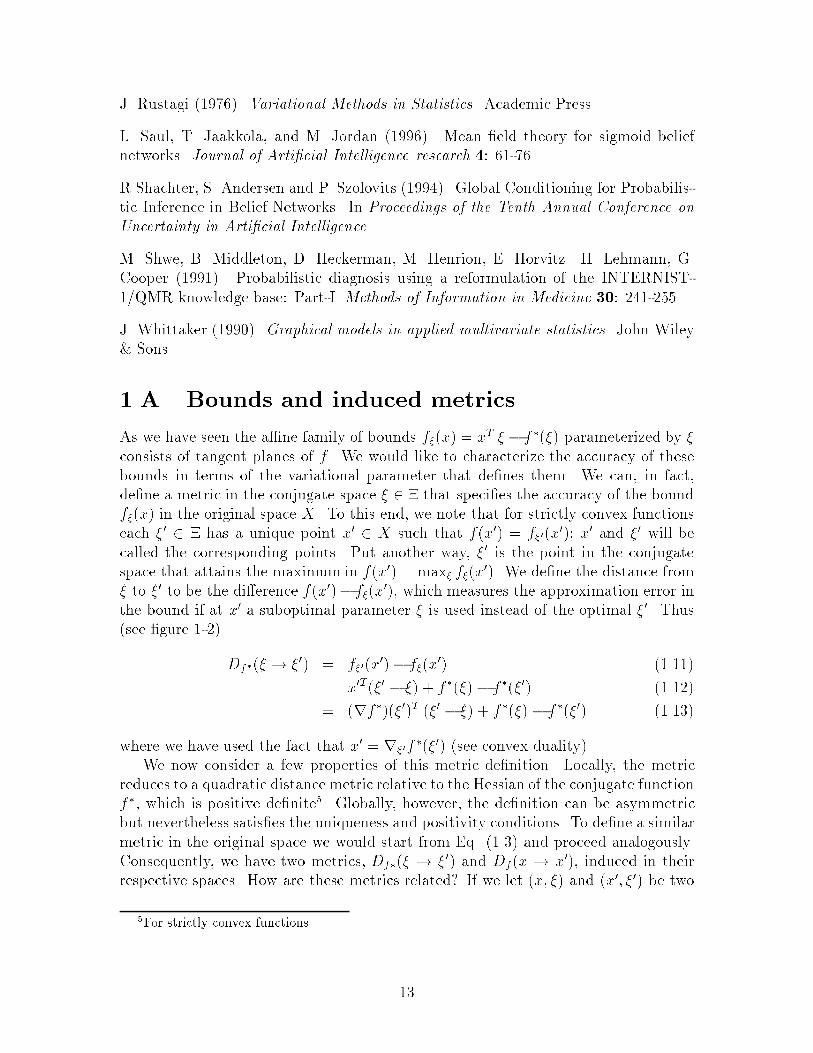
J. Rustagi (1976). Variational Methods in Statistics. Academic Press.L. Saul, T. Jaakkola, and M. Jordan (1996). Mean �eld theory for sigmoid beliefnetworks. Journal of Arti�cial Intelligence research 4: 61-76.R Shachter, S. Andersen and P. Szolovits (1994). Global Conditioning for Probabilis-tic Inference in Belief Networks. In Proceedings of the Tenth Annual Conference onUncertainty in Arti�cial Intelligence.M. Shwe, B. Middleton, D. Heckerman, M. Henrion, E. Horvitz. H. Lehmann, G.Cooper (1991). Probabilistic diagnosis using a reformulation of the INTERNIST-1/QMR knowledge base: Part-I. Methods of Information in Medicine 30: 241-255.J. Whittaker (1990). Graphical models in applied multivariate statistics. John Wiley& Sons.1.A Bounds and induced metricsAs we have seen the a�ne family of bounds f�(x) = xT � � f�(�) parameterized by �consists of tangent planes of f . We would like to characterize the accuracy of thesebounds in terms of the variational parameter that de�nes them. We can, in fact,de�ne a metric in the conjugate space � 2 � that speci�es the accuracy of the boundf�(x) in the original space X. To this end, we note that for strictly convex functionseach �0 2 � has a unique point x0 2 X such that f(x0) = f�0(x0); x0 and �0 will becalled the corresponding points. Put another way, �0 is the point in the conjugatespace that attains the maximum in f(x0) = max� f�(x0). We de�ne the distance from� to �0 to be the di�erence f(x0)� f�(x0), which measures the approximation error inthe bound if at x0 a suboptimal parameter � is used instead of the optimal �0. Thus(see �gure 1-2) Df�(� ! �0) = f�0(x0)� f�(x0) (1.11)= x0T(�0 � �) + f�(�) � f�(�0) (1.12)= (rf�)(�0)T (�0 � �) + f�(�) � f�(�0) (1.13)where we have used the fact that x0 = r�0f�(�0) (see convex duality).We now consider a few properties of this metric de�nition. Locally, the metricreduces to a quadratic distance metric relative to the Hessian of the conjugate functionf�, which is positive de�nite5. Globally, however, the de�nition can be asymmetricbut nevertheless satis�es the uniqueness and positivity conditions. To de�ne a similarmetric in the original space we would start from Eq. (1.3) and proceed analogously.Consequently, we have two metrics, Df�(� ! �0) and Df (x ! x0), induced in theirrespective spaces. How are these metrics related? If we let (x; �) and (x0; �0) be two5For strictly convex functions 13

x x’

D(ξ→ξ’)

f(x)

x ξ - f*(ξ)

x ξ’ - f*(ξ’)Figure 1-2: The de�nition of the dual (semi)metric.pairs of corresponding points, then we have the equalityDf (x! x0) = Df�(�0 ! �) (1:14)This indicates that the induced (directional) distance in the original space is equal tothe induced distance in the dual space but in the reverse direction. More generally,the length of a path in the original space is equal to the length of the reverse path inthe dual space. The de�nition of D above thus generates a meaningful dual metric.Let us consider a few examples. We start from a simple one where f(x) = x2=2,which is a convex function. The conjugate of f can be found from Eq. (1.3)f�(�) = maxx f x � � 12x2 g = 12�2 (1:15)and it has the same quadratic form. According to Eq. (1.13), this representationinduces a metric in the original x space (note that unlike before we are now consideringthe bounds on the conjugate rather than the original function). This metric isDf (x! x0) = (rf)T (x0) (x0 � x) + f(x)� f(x0) (1.16)= x0(x0 � x) + 12x2 � 12x02 = 12(x0 � x)2 (1.17)which is the usual Euclidean metric. This result can be generalized to quadratic formsde�ned by a positive de�nite matrix.As another example, let us consider the negative entropy function f(p) = �H(p),which is convex in the space of probability distributions (see e.g., Cover & Thomas1991). The conjugate to this function is given byf�(�) = maxp f pT �� (�H(p)) g (1.18)= maxp fXi pi�i �Xi pi log pi g (1.19)= maxp fXi pi log e �ipi g = logXi e �i (1.20)14

where we have carried out the maximization analytically; the maximum is attained forpi / e �i which is the Boltzmann distribution. We note that the conjugate function {the log partition function { has to be a convex function of � (the conjugates of convexfunctions are convex). We are now able to ask what the induced metric is in the pspace. Using the de�nition above we obtainDf (p! p0) = (rf)T (p0) (p0 � p) + f(p) � f(p0) (1.21)= Xi (p0i � pi) log p0i �H(p) +H(p0) (1.22)= Xi pi log pip0i = KL(p; p0) (1.23)which is the KL-divergence between the distributions p and p0. We note that log-partition functions will appear frequently in the thesis and thus whenever the repre-sentation Eq. (1.18) is used to lower bound them, the associated metric will be theKL-distance. The associated metrics for all other transformations appearing in thethesis can be obtained analogously.

15

Chapter 2Upper and lower bounds12.1 IntroductionWhile Monte Carlo methods approximate probabilities in a stochastic sense, we de-velop deterministic methods that yield strict lower and upper bounds for marginalprobabilities in graphical models. These bounds together yield interval bounds on thedesired probabilities. Although the problem of �nding such intervals to predescribedaccuracy is NP-hard in general (Dagum and Luby 1993), bounds that can be com-puted e�ciently may nevertheless yield intervals that are accurate enough to be usefulin practice.Previous work on interval approximations include Draper and Hanks (1994) (seealso Draper 1995) where they extended Pearl's polytree algorithm (Pearl 1988) topropagate interval estimates instead of exact probabilities in polytrees. Their method,however, relies on the polytree property for e�ciency and does not (currently) gen-eralize feasibly to densely connected networks. We focus in this work particularly onnetwork models with dense connectivity.Dense connectivity leads not only to long execution times but may also involveexponentially many parameters that must be assessed or learned. The latter issueis generally addressed via parsimonious representations such as the logistic sigmoid(Neal 1992) or the noisy-OR function (Pearl 1988). In order to retain the compact-ness of these representations throughout our inference and estimation algorithms, wedispense with the moralization and triangulation procedures of the exact (clustering)framework and operate on the given graphical model directly.We develop our interval approximation techniques for a class of networks that wecall log-concave models. These models are characterized by their convexity propertiesand include sigmoid belief networks and noisy-OR networks as special cases. Previouswork on sigmoid belief networks (Saul et al. 1996) provided a rigorous lower bound;we complete the picture here for these models by deriving the missing upper bound.We also present upper and lower bounds for the more general class of log-concave1The basic content of this chapter has previously appeared in \T. Jaakkola and M. Jordan (1996).Computing upper and lower bounds on likelihoods in intractable networks. In Proceedings of thetwelfth Conference on Uncertainty in Arti�cial Intelligence".16

models focusing on noisy-OR networks in particular. While the lower bounds weobtain are applicable to generic network structures, the upper bounds we derive hereare restricted to two-level (or bipartite) networks. The extension of the upper boundsto more general networks will be addressed in chapter 3. There are neverthelessmany potential applications for the restricted bounds, including the probabilisticreformulation of the QMR knowledge base (Shwe et al. 1991) that will be consideredin detail in chapter 5. The emphasis of this chapter is on techniques of boundingand their analysis rather than on all{encompassing inference algorithms. Mergingthe bounding techniques with exact calculations can yield a considerable advantage,as will be evident in chapter 5 (see chapter 3 for more general methodology).The current chapter is structured as follows. Section 2.2 introduces the log-concavemodels and develops the techniques for upper and lower bounds. Section 2.3 containsan application of these techniques to sigmoid networks and gives a preliminary nu-merical analysis of the accuracy of the obtained bounds. Section 2.4 is devoted anal-ogously for noisy-OR networks. We then summarize the results and describe somefuture work.2.2 Log-concave modelsWe consider here a class of acyclic probabilistic networks de�ned over binary (0/1)variables S1; : : : ; Sn. The joint probability distribution over these variables has theusual decompositional structure:P (S1; : : : ; Snj�) =Yi P (SijSpai; �i) (2.1)where Spai is the set of parents of Si. The conditional probabilities, however, areassumed to have the following restricted formP (SijSpai; �) = GSi 0@ �i0 + Xj2pai �ijSj 1A (2.2)where logG0(x) and logG1(x) are both concave functions of x. The parametersspecifying these conditional probabilities are the real valued \weights" �ij. We referto networks conforming to these constraints as log-concave models. While this class ofmodels is restricted, it nevertheless contains sigmoid belief networks (Neal, 1992) andnoisy-OR networks (Pearl, 1988) as special cases. The particulars of both sigmoidand noisy-OR networks will be considered in later sections.In the remainder of this section we present techniques for computing upper andlower bounds on marginal probabilities in log-concave networks. We note that anysuccessful instantiation of evidence in these networks relies on the ability to estimatesuch marginals. The upper bounds that we derive are restricted to two-level (bipar-tite) networks while the lower bounds are valid for arbitrary network structures.17

. . .

. . . L1

L 2Figure 2-1: Two level (bipartite) network.2.2.1 Upper bound for log-concave networksWe restrict our attention here to two-level directed architectures. For clarity we dividethe variables in these two levels as observable (level 1 or L1) and latent variables (level2 or L2). See �gure 2-1 for an example. The bipartite structure of these networksimplies (i) that the latent variables are marginally independent, and (ii) the observablevariables are conditionally independent. The joint distribution for log-concave modelswith this special architecture is given byP (S1; : : : ; Snj�) = Yi2L1GSi 0@�i0 + Xj2pai �ijSj1A Yj2L2 P (Sj j�j) (2.3)where L1 and L2 signify the two layers (observable and latent). Note that the con-nectivity is from L2 (latent variables) to L1 (observables).To compute the marginal probability of a set of variables in these networks wenote that (i) any latent variable included in this desired marginal set only reducesthe complexity of the calculations, and (ii) the form of the architecture makes thoseobservable variables (in L1) that are excluded from the desired marginal set inconse-quential. We will thus adopt a simplifying notation in which the marginal set consistsof all and only the observable variables (i.e., those in L1). The goal is therefore tocompute P (fSigi2L1j�) = XfSjgj2L2 P (S1; : : : ; Snj�) (2.4)Given our assumption that computing such marginal probability is intractable, weseek an upper bound instead. The goal is to simplify the joint distribution such thatthe marginalization across L2 or latent variables can be accomplished e�ciently, whilemaintaining at all times a rigorous upper bound on the desired marginal probability.We develop variational transformations for this purpose. The transformations weconsider come from convex duality as explained previously in section 1.1.To use such variational bounds in the context of probabilistic calculations, we re-call the concavity property of our conditional probabilities (on a log-scale). Accordingto convex duality, we can �nd a variational bound of the formlogGSi 0@�i0 + Xj2pai �ijSj1A � �i0@�i0 + Xj2pai �ijSj1A� f�(�i) (2.5)18

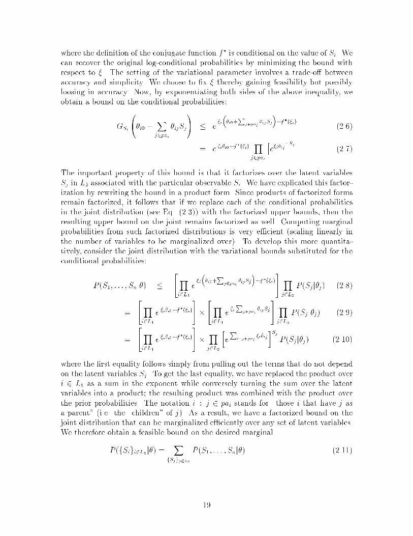
where the de�nition of the conjugate function f� is conditional on the value of Si. Wecan recover the original log-conditional probabilities by minimizing the bound withrespect to �. The setting of the variational parameter involves a trade-o� betweenaccuracy and simplicity. We choose to �x � thereby gaining feasibility but possiblyloosing in accuracy. Now, by exponentiating both sides of the above inequality, weobtain a bound on the conditional probabilities:GSi 0@�i0 + Xj2pai �ijSj1A � e �i��i0+Pj2pai �ijSj��f�(�i) (2.6)= e �i�i0�f�(�i) Yj2pai he�i�ijiSj (2.7)The important property of this bound is that it factorizes over the latent variablesSj in L2 associated with the particular observable Si. We have explicated this factor-ization by rewriting the bound in a product form. Since products of factorized formsremain factorized, it follows that if we replace each of the conditional probabilitiesin the joint distribution (see Eq. (2.3)) with the factorized upper bounds, then theresulting upper bound on the joint remains factorized as well. Computing marginalprobabilities from such factorized distributions is very e�cient (scaling linearly inthe number of variables to be marginalized over). To develop this more quantita-tively, consider the joint distribution with the variational bounds substituted for theconditional probabilities:P (S1; : : : ; Snj�) � 24Yi2L1 e �i��i0+Pj2pai �ijSj��f�(�i)35 Yj2L2 P (Sjj�j) (2.8)= 24Yi2L1 e �i�i0�f�(�i)35� 24Yi2L1 e �iPj2pai �ijSj35 Yj2L2 P (Sj j�j) (2.9)= 24Yi2L1 e �i�i0�f�(�i)35� Yj2L2 �ePi : j2pai �i�ij�Sj P (Sj j�j) (2.10)where the �rst equality follows simply from pulling out the terms that do not dependon the latent variables Sj. To get the last equality, we have replaced the product overi 2 L1 as a sum in the exponent while conversely turning the sum over the latentvariables into a product; the resulting product was combined with the product overthe prior probabilities. The notation i : j 2 pai stands for \those i that have j asa parent" (i.e. the \children" of j). As a result, we have a factorized bound on thejoint distribution that can be marginalized e�ciently over any set of latent variables.We therefore obtain a feasible bound on the desired marginalP (fSigi2L1j�) = XfSjgj2L2 P (S1; : : : ; Snj�) (2.11)19

� 24Yi2L1 e �i�i0�f�(�i)35� Yj2L2 �ePi : j2pai �i�ijPj + 1� Pj� (2.12)where for clarity we have used the notation Pj = P (Sj = 1j�j). Before touching thequestion of how to optimally set the variational parameters, we make a few generalobservations about this bound. First, the bound is never vacuous, i.e., there alwaysexists a setting of the variational parameters such that the bound is less than or equalto one. To see this, let �i = 0 for all i 2 L1. The bound in this case becomes simplyYi2L1 e�f�(0) (2.13)We can now make use of the property that for every2 � there exist an x such that thebound is exact at that point. If we let x0 be this point for � = 0, then logGSi (x0) =x0 0� f�(0) = �f�(0). Putting this back into the reduced bound givesYi2L1 e logGSi (x0) = Yi2L1GSi(x0) (2.14)As all GSi(x0) are conditional probabilities, the product has to remain less thanor equal to one. Second, we note (without a proof) that in the limit of vanishinginteraction parameters �ij between the layers, the bound becomes exact. Also, sincethe variational bounds can be viewed as tangents, small variations in �ij around zeroare (always) captured accurately.We now turn to the question of how to optimize the variational parameters. Dueto the products involved, the bound is easier to handle in log-scale, and we writelogP (fSigi2L1j�) � Xi2L1 [�i�i0 � f�(�i)] + Xj2L2 log �ePi : j2pai �i�ijPj + 1 � Pj� (2.15)In order to make this bound as tight as possible, we need to minimize the bound withrespect to �. Importantly, this minimization problem is convex in the variationalparameters � (see below). The implication is that there are no local minima, and theoptimal parameter settings can be always found through standard procedures suchas Newton-Raphson. Let us now verify that the bound is indeed a convex functionof the variational parameters �. The convexity of �f�(�i) follows directly from theconcavity of the conjugate functions f�. The convexity oflog �ePi : j2pai �i�ijPj + 1� Pj� (2.16)follows from a more general convexity property well-known in the physics literature:f(r) = logEX ner(X)o (2.17)2The variational parameter may have a restricted set of possible values, but in the context of thelog-concave models considered here, the value zero is in the admissible set.20

is a convex functional of r (see Appendix 2.A for a simple proof). The expectationpertains to the random variable X. In our case the expectation is over Sj takingvalues in f0; 1g with probabilities 1 � Pj and Pj. The function r corresponds toPi : j2pai �i�ijSj, and since a�ne transformations do not alter convexity properties,convexity in r implies convexity in �.2.2.2 Generic lower bound for log-concave networksMethods for �nding lower bounds on marginal likelihoods were �rst presented byDayan et al. (1995) and Hinton et al. (1995) in the context of a layered networkknown as the \Helmholtz machine". Saul et al. (1996) subsequently provided a morerigorous calculation of these lower bounds (by appeal to mean �eld) in the case ofgeneric sigmoid networks. Unlike the method presented earlier for obtaining upperbounds presented in the previous section, this lower bound methodology poses noconstraints on the network structure. The restriction on the upper bounds will beremoved in chapter 3.We provide here an alternative derivation of the lower bounds, one that establishesthe connection to convex duality similarly to the upper bounds. Consider thereforethe problem of computing a log-marginal probability logP (S�):logP (S�) = logXS P (S; S�) = logXS e logP (S;S�) = logXS e r(S) = f(r) (2.18)where S and S� denote two sets of variables, and the summation is over the possiblecon�gurations of the variables in the set S. The function r is de�ned as r(S) =logP (S; S�). We can now use the previously established result that f(r) is convexin r. Analogously to upper bounds, convex duality now implies that we can �nd abound f(r) = logXS e r(S) � XS q(S)r(S)� f�(q) (2.19)= XS q(S) logP (S; S�)� f�(q) (2.20)= XS q(S) logP (S; S�) +H(q) (2.21)which is exact if maximized over the variational distribution3 q. The conjugate func-tion f� turns out to be the negative entropy �H(q) of the q distribution (see Ap-pendix 1.A). Unlike with upper bounds, the variational parameters are now quitecomplex, i.e., distributions over a set of variables. The optimal variational distribu-tion q�(S) = P (SjS�), the one that attains the maximum, is often infeasible to usein the bound. The choice of the variational distribution therefore involves a trade-o�between feasibility and accuracy, where the accuracy is characterized by an inherenterror metric associated with these convexity bounds (see the appendix of chapter 1).3The fact that the variational parameters de�ne a probability distribution is speci�c to the casewe are considering. 21

In this case, the metric specifying the loss in accuracy due to a suboptimal choicefor q is the Kullback-Leibler distance between q and the optimal distribution q� (seeAppendix 1.A). To emphasize feasibility we consider a particularly tractable (butnaturally suboptimal) class of variational distributions, that of completely factorizeddistributions: q(S) =Yi qi(Si) (2.22)We can insert this form into the lower bound of Eq. (2.21) and consequently adjustthe parameters in q (the component distributions) to make the bound as tight aspossible. The resulting approximation is known as the mean �eld approximation (seee.g. Saul, et al., 1996). We note that in contrast to the upper bound, the mean�eld lower bound is not guaranteed to be free of local maxima. Furthermore, even inthe case of mean �eld distributions, it may not be trivial to evaluate the associatedbound. While the entropy term in this case reduces to a manageable expression givenby H(q) =Xi H(qi) = �Xi XSi qi(Si) log qi(Si); (2.23)the same is not necessarily true for the �rst term in Eq. (2.21). For example, in thecontext of our log-concave models, the lower bound is given byXi XS q(S) logGSi 0@�i0 + Xj2pai �ijSj1A+H(q)= Xi Eq logGSi 0@�i0 + Xj2pai �ijSj1A +H(q) (2.24)where the sum over i follows from the product decomposition of the joint distri-bution, and the expectation is with respect to the mean �eld distribution q. Thenon-linearities in the log-conditional probabilities (i.e. in logGSi) may render the ex-pectation over the \latent" variables S exponentially costly in the number of parentsof Si (almost regardless of the form of the distribution q). Additional approximationsor bounds are therefore often necessary even with the mean �eld approximation.These approximations, however, make use of the particulars of the models and wewill consider them separately for sigmoid and noisy-OR networks. Note that the sim-plicity o�ered by the mean �eld distribution greatly facilitates the derivation of theseadditional approximations.22

2.3 Sigmoid belief networksSigmoid belief networks belong to the class of log-concave models considered earlier.The conditional probabilities for sigmoid networks take the formP (SijSpai; �) = g 0@�i0 + Xj2pai �ijSj1ASi 241 � g0@�i0 + Xj2pai �ijSj1A351�Si (2.25)where g(x) = 1=(1+exp(�x)) is the logistic function (also called a \sigmoid" functionbased on its graphical shape; see Figure 2-6). The required log-concavity propertyfollows from the fact that both log g(x) and log(1 � g(x)) = log g(�x) are concavefunctions of x. We note that the choice of the above dependency model is not ar-bitrary but is rooted in logistic regression in statistics (McCullagh & Nelder, 1983).Furthermore, this form of dependency corresponds to the assumption that the oddsfrom each parent of a node combine multiplicatively; the weights �ij in this interpre-tation bear a relation to log-odds.We now adapt the generic results for log-concave models to sigmoid networks andevaluate them numerically. We start with the upper bound.2.3.1 Upper bound for sigmoid networkIn order to obtain an upper for the class of two-level sigmoid networks we needto specify the exact form of the variational transformation used in Eq. (2.5) andconsequently in Eq. (2.15) for log-concave models. For sigmoid networks this meansto quantify the transformation of log g(x) (cf. the probability model). The derivationof this transformation is presented in Appendix 2.B. As a result we obtainlogGSi 0@�i0 + Xj2pai �ijSj1A � (Si � �i)0@�i0 + Xj2pai �ijSj1A �H(�i) (2.26)where H(�) is the binary entropy function. Note that we have explicated how thetransformation depends on the value of Si (unlike in the case of the generic trans-formation of Eq. (2.5), where the dependence was left implicit). We may now usethe above transformation in Eq. (2.15) to get the desired bound on the log-marginalprobability:log P (fSigi2L1j�) � Xi2L1 [(Si � �i)�i0 �H(�i)]+ Xj2L2 log �ePi : j2pai(Si��i)�ijPj + 1� Pj� (2.27)As described earlier the optimal setting of the variational parameters � can be foundsimply via the standard Newton-Raphson method.23

2.3.2 Generic lower bound for sigmoid networkOur derivation of lower bounds for sigmoid networks deviates from those presented inSaul et al. (1996) in terms of the type of additional approximations used to facilitatethe evaluation of the lower bound. Let us therefore describe brie y the techniquesthat we use as they correspond to the numerical results presented in the followingsection. We refer the reader to Saul et al. for their method. To this end, recall�rst that the evaluation of the lower bound involves performing averages over log-conditional probabilities with respect to the mean �eld distribution (see Eq. (2.24)).For sigmoid networks this means averages of the formEq logGSi(Xi) = Eq f SiXi + log g(�Xi) g (2.28)where we have used the notation Xi = �i0 +Pj2pai �ijSj and the identityGSi(Xi) = g(Xi)Si(1� g(Xi))1�Si = " g(Xi)1 � g(Xi)#Si (1 � g(Xi)) (2.29)= e SiXi g(�Xi) (2.30)particular to sigmoid networks. Given that the mean �eld distribution q is factor-ized, the only di�culty in evaluating the expectations above comes from the termEq log g(�Xi). To alleviate this problem we resort to an additional variational trans-formation of log g(�Xi), one that yields a lower bound (cf. the upper bound trans-formation presented earlier). This transformation is derived in Jaakkola & Jordan(1996) (see Appendix 3.B) and is given bylog g(�Xi) � �(Xi � �i)=2 � �(�)(X2i � �2i ) + log g(��i) (2.31)where �(�) = tanh(�=2)=(4�), and the transformation is exact whenever �i = Xi.This additional lower bound depends on Xi only quadratically and can be readilyaveraged over the factorized mean �eld distribution.2.3.3 Numerical experiments for sigmoid networkIn testing the accuracy of the developed bounds we used 8! 8 networks (complete bi-partite graphs as in Figure 2-1 with 8 nodes in each level), where the network size waschosen to be small enough to allow exact computation of the marginal probabilitiesfor purposes of comparison. The method of testing was as follows. The parametersfor the 8! 8 networks were drawn from a Gaussian prior distribution and a samplefrom the resulting joint distribution of the variables was generated. The variables inthe \receiving" layer of the bipartite graph were set according to the sample. Thetrue marginal probability as well as the upper and lower bounds were computed forthis setting. The resulting bounds were assessed by employing the relative error inlog-likelihood, i.e. (log PBound= log P � 1), as a measure of accuracy.24

More precisely, the prior distribution over the parameters was taken to beP (�) =Yi Yj2pai 1p2��2 e� 12�2 �2ij (2:32)where the overall variance �2 allows us to vary the degree to which the resultingparameters make the two layers of the network dependent. For small values of �2 thelayers are almost independent whereas larger values make them strongly interdepen-dent. To make the situation worse for the bounds4 we enhanced the coupling of thelayers by setting P (Sjj�j) = 1=2 for the variables not in the desired marginal set, i.e.,making them maximally variable.In order to make the accuracy of the bounds commensurate with those for thenoisy-OR networks reported below, we summarize the results via a measure of inter-layer dependence. This dependence was estimated by�std = maxi2L1 qVarfP (SijSpai)g (2:33)i.e., the maximum variability of the conditional likelihoods. Here Si was �xed in theP (SijSpai) functional according to the initial sample and the variance was computedwith respect to the joint distribution5.Figure 2-2 illustrates the accuracy of the bounds as measured by the relativelog-likelihood as a function of �std6. In terms of probabilities, a relative error of �translates into a P 1+� approximation of the true likelihood P . Note that the relativeerror is always positive for the upper bound and negative for the lower bound, asguaranteed by the theory. The �gure indicates that the bounds are accurate enoughto be useful. In addition, we see that the the upper bound deteriorates faster withincreasingly coupled layers.Let us now brie y consider the scaling properties of the bounds as the networksize increases. We note �rst that the evaluation time for the bounds increases ap-proximately linearly with the number of parameters � in these two-level networks7.The accuracy of the bounds, on the other hand, needs experimental illustration.In large networks it is not feasible to compute �std nor the true marginal likelihood.We may, however, calculate the relative error between the upper and lower bounds.To maintain approximately same level of �std across di�erent network sizes we plottedthe errors against �pn (for fully connected n by n two-level networks), where � isthe overall standard deviation in the prior distribution. Figure 2-3 shows that therelative errors are invariant to the network size in this scaling.4Both the upper and lower bounds are exact in the limit of lightly coupled layers.5Note that P (SijSpai) with Si �xed is just some function of the variables in the network whosevariance can be computed.6Note that the maximum value for �std is 1=2.7The amount of computation needed for sequentially optimizing each variational parameter oncescales linearly with the number of network parameters. Only a few such iterations are needed.25

0.05 0.1 0.15 0.2 0.25−0.1

−0.05

0

0.05

0.1

Figure 2-2: Sigmoid networks. Accuracy of the bounds for 8 by 8 two-level networks.The solid lines are the median relative errors in log-likelihood as a function of �std.The upper and lower curves correspond to the upper and lower bounds respectively.0 0.5 1 1.5 2

0

0.05

0.1

0.15

Figure 2-3: Sigmoid networks. Median relative errors between the upper and lowerbounds (log scale) as a function of �n 12 for n by n two-level networks. Solid line:n = 8; dashed line: n = 32; dotted line: n = 128.2.4 Noisy-OR networkNoisy-OR networks { like sigmoid networks { are log-concave models. In de�ningthe conditional probabilities for noisy-OR networks we deviate somewhat from thestandard notation to reveal the relation to log-concave models and for clarity of theforthcoming expressions. In our notation the conditional probabilities are written asP (SijSpai; �) = �1� e�[�i0+Pj2pai �ijSj ]�Si �e�[�i0+Pj2pai �ijSj]�1�Si (2.34)where all the weights �ij are non-negative. The connection to the standard notation isvia �ij = � log(1 � qij), where qij is the probability corresponding to the propositionthat the jth parent alone can turn Si on. qi0 (related to the bias in our notation)has a special interpretation as a leak probability, i.e., the probability that something26

other than the parents can independently turn Si on. The log-concavity feature ofthis probability model stems from the concavity of log(1� e�x).As with sigmoid networks we now adapt the general results to noisy-OR networksand verify the accuracy of the bounds numerically.2.4.1 Upper bound for noisy-OR networkTo specify the variational transformation of the noisy-OR conditional probabilities,we only need to consider the transformation of logG1(x) = log(1�e�x) since logG0(x)already has a linear form (see the probability model). Details are given in Appendix2.C. By combining the transformation and the linear form, we �ndlogGSi 0@�i0 + Xj2pai �ijSj1A � (Si�i + Si � 1)0@�i0 + Xj2pai �ijSj1A � Sif�(�i) (2.35)where f�(�i) = �i log �i � (� + 1) log(�1 + 1). We have again written explicitly thedependency on the value of Si. This transformation leads to the following log-marginalbound (see Eq. (2.15)):logP (fSigi2L1j�) � Xi2L1 [(Si�i + Si � 1)�i0 � Sif�(�i)]+ Xj2L2 log �ePi : j2pai(Si�i+Si�1)�ijPj + 1� Pj� (2.36)The log-bound is convex in the variational parameters and can be optimized by appealto standard methods.2.4.2 Generic lower bound for noisy-OR networkThe earlier work on lower bounds by Saul et al. was restricted to sigmoid networks; weextend that work here by deriving a lower bound for generic noisy-OR networks. Werefer to section 2.2.2 for the framework and commence from the noisy-OR counterpartof eq. (2.21). For clarity, we use the notation Xi = �i0 +Pj2pai �ijSj and �ndlog P � Xi Eq logGSi(Xi) +H(q) (2.37)= Xi Eq n Si log(1 � e�Xi) o+Xi Eq f �(1 � Si)Xi g+H(q) (2.38)which comes from using the form of the conditional probabilities for noisy-OR net-works; logP is a shorthand for the log-marginal we are trying to compute. Whilethe second (mean �eld) expectation in eq. (2.38) simply corresponds to replacing thebinary variable Si and those in the linear form Xi with their \means" qi 8, the �rstexpectation lacks a closed form expression. To compute this expectation e�ciently8For simplicity we denote qi(Si = 1) by qi. 27

we make use of the following expansion:1� e�x = 1Yk=0 g(2kx) (2:39)where g(�) is the sigmoid function (see Appendix 2.D for details). This expansionconverges exponentially fast and thus only a few terms need to be included in theproduct for good accuracy. By carrying out this expansion in the bound above andexplicitly using the form of the sigmoid function we getlogP � Xi Xk Eq n�Si log(1 + e�2kXi) o�Xi (1� qi)Xj �ijqj +H(q) (2.40)Now, as the parameters �ij are non-negative, Xi = �i0 +Pj2pai �ijSj � 0, ande�2kXi 2 [0; 1] (2.41)We may therefore use the smooth convexity properties of � log(1+ x) (for x 2 [0; 1])to bring the expectations in eq. (2.40) inside the log. This results inlog P � �Xik qi log 241 + e�2k�i0 Yj2pai(qje�2k�ij + 1� qj)35�Xi (1� qi) Xj2pai �ijqj +H(q) (2.42)A more sophisticated and accurate way of computing the expectations in eq. (2.40)is discussed in Appendix 2.E.2.4.3 Numerical experiments for noisy-OR networkThe method of testing used here was, for the most part, identical to the one presentedearlier for sigmoid networks (section 2.3.3). The only di�erence was that the priordistribution over the parameters de�ning the conditional probabilities was chosen tobe an exponential instead of a Gaussian:�ij � � e���ij (2.43)(this corresponds to a Dirichlet distribution over the parameters in the standard noisy-OR notation). For large �, �ij stays small and the layers of the bipartite networkare only weakly connected; smaller values of �, on the other hand, make the layersstrongly dependent. We thus used � to vary (on average) the interdependence betweenthe two layers. To facilitate comparisons with the bounds derived for sigmoid networkswe used �std (see eq. (2.33)) as a measure of dependence between the layers.28

Figure 2-4 illustrates the accuracy of the computed bounds as a function of �std9.The samples with zero relative error are from the upper/lower bounds in cases whereall the variables in the desired marginal are zero since the bounds become exactwhenever this happens. The lower bound is slightly worse than the one for sigmoidnetworks most likely due to the symmetry and smoother nature of the sigmoid func-tion. As with the sigmoid networks the upper bound becomes less accurate morequickly.We now turn to the e�ects of increasing the network size. Analogously to thesigmoid networks the evaluation times for the bounds vary approximately linearlywith the number of parameters in these two-level networks, albeit with slightly largercoe�cients (for the lower bound). As for the accuracy of the bounds, Figure 2-5shows the relative errors10 between the bounds across di�erent network sizes. Theerrors are plotted against pn=� for n by n two-level networks, where � de�nes theexponential prior distribution for the parameters. In the chosen scale the networksize has little e�ect on the errors11.0.05 0.1 0.15 0.2 0.25

−0.1

−0.05

0

0.05

0.1

Figure 2-4: Noisy-OR network. Accuracy of the bounds for 8 by 8 two-level networks.The solid lines are the median relative errors in log-likelihood as a function of �std.The upper and lower curves correspond to the upper and lower bounds respectively.2.5 Discussion and future workApplying probabilistic methods to real world inference problems can lead to the emer-gence of cliques that are prohibitively large for exact algorithms (for example, inmedical diagnosis). We focused on dealing with such large (sub)structures in thecontext of a class of networks we call log-concave models with an emphasis on thesigmoid and noisy-OR realizations. For these networks we developed techniques for9The slight unevenness of the samples are due to the non-linear relationship between the param-eter � for the exponential distribution and �std.10The errors are for the worst case marginal, i.e., for P (fSi = 1gi2L1).11The 8 by 8 network is too small to be in the desired asymptotic regime.29

0 0.02 0.04 0.06 0.080

0.02

0.04

0.06

0.08

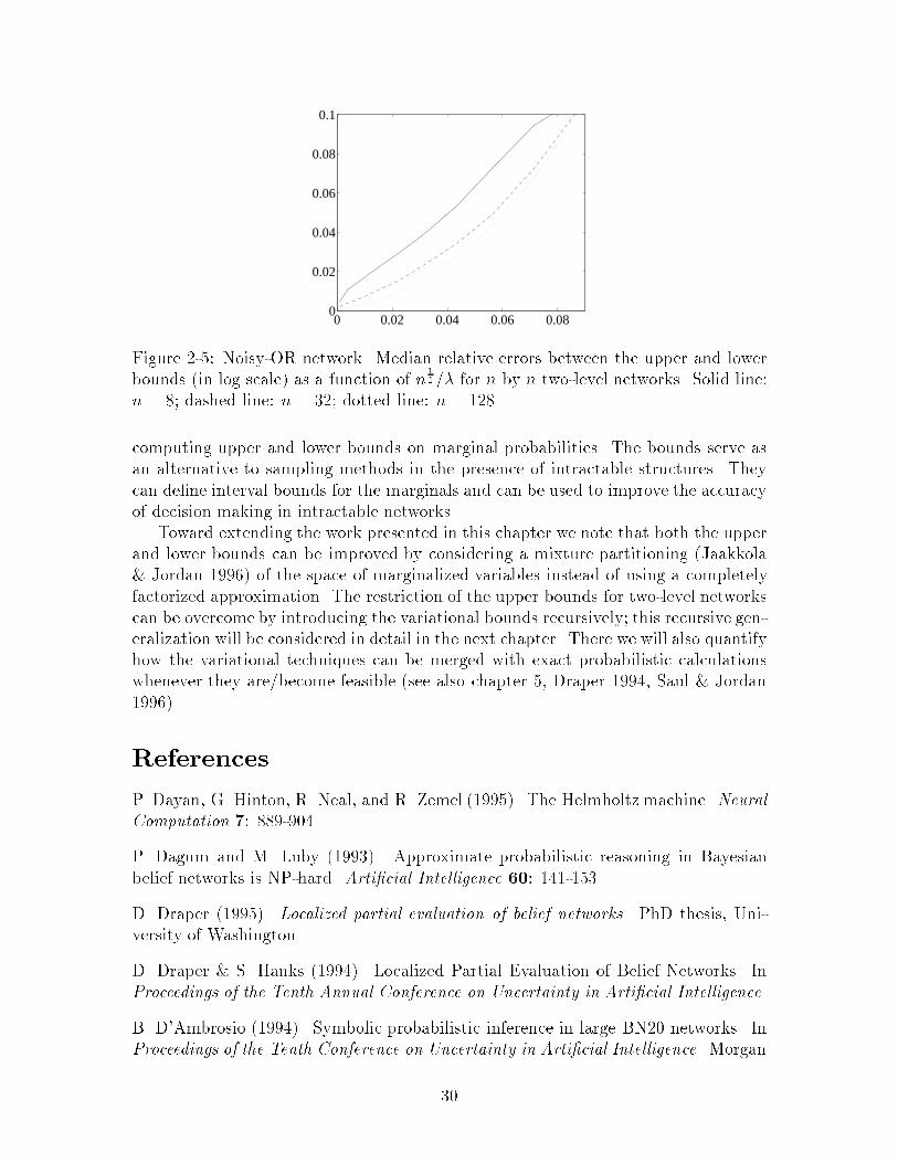
0.1

Figure 2-5: Noisy-OR network. Median relative errors between the upper and lowerbounds (in log scale) as a function of n 12=� for n by n two-level networks. Solid line:n = 8; dashed line: n = 32; dotted line: n = 128.computing upper and lower bounds on marginal probabilities. The bounds serve asan alternative to sampling methods in the presence of intractable structures. Theycan de�ne interval bounds for the marginals and can be used to improve the accuracyof decision making in intractable networks.Toward extending the work presented in this chapter we note that both the upperand lower bounds can be improved by considering a mixture partitioning (Jaakkola& Jordan 1996) of the space of marginalized variables instead of using a completelyfactorized approximation. The restriction of the upper bounds for two-level networkscan be overcome by introducing the variational bounds recursively; this recursive gen-eralization will be considered in detail in the next chapter. There we will also quantifyhow the variational techniques can be merged with exact probabilistic calculationswhenever they are/become feasible (see also chapter 5, Draper 1994, Saul & Jordan1996).ReferencesP. Dayan, G. Hinton, R. Neal, and R. Zemel (1995). The Helmholtz machine. NeuralComputation 7: 889-904.P. Dagum and M. Luby (1993). Approximate probabilistic reasoning in Bayesianbelief networks is NP-hard. Arti�cial Intelligence 60: 141-153.D. Draper (1995). Localized partial evaluation of belief networks. PhD thesis, Uni-versity of Washington.D. Draper & S. Hanks (1994). Localized Partial Evaluation of Belief Networks. InProceedings of the Tenth Annual Conference on Uncertainty in Arti�cial Intelligence.B. D'Ambrosio (1994). Symbolic probabilistic inference in large BN20 networks. InProceedings of the Tenth Conference on Uncertainty in Arti�cial Intelligence. Morgan30

Kaufmann.G. Hinton, P. Dayan, B. Frey, and R. Neal (1995). The wake-sleep algorithm forunsupervised neural networks. Science 268: 1158-1161.D. Heckerman (1989). A tractable inference algorithm for diagnosing multiple dis-eases. In Proceedings of the Fifth Conference on Uncertainty in Arti�cial Intelligence.Morgan Kaufmann.T. Jaakkola, L. Saul, and M. Jordan (1996). Fast learning by bounding likelihoodsin sigmoid-type belief networks. To appear in Advances of Neural Information Pro-cessing Systems 8. MIT Press.T. Jaakkola and M. Jordan (1996). Mixture model approximations for belief networks.Manuscript in preparation.F. Jensen, S. Lauritzen, and K. Olesen (1990). Bayesian updating in causal probabilis-tic networks by local computations. Computational Statistics Quarterly 4: 269-282.S. Lauritzen and D. Spiegelhalter (1988). Local computations with probabilities ongraphical structures and their application to expert systems. Journal of the RoyalStatistical Society B 50:154-227.P. McCullagh & J. Nelder (1983). Generalized linear models. Chapman and Hall.R. Neal. Connectionist learning of belief networks (1992). Arti�cial Intelligence 56:71-113.J. Pearl (1988). Probabilistic Reasoning in Intelligent Systems. Morgan Kaufmann.L. Saul, T. Jaakkola, and M. Jordan (1996). Mean �eld theory for sigmoid beliefnetworks. Journal of Arti�cial Intelligence Research 4: 61-76.L. Saul and M. Jordan (1996). Exploiting tractable substructures in intractablenetworks. To appear in Advances of Neural Information Processing Systems 8. MITPress.M. Shwe, B. Middleton, D. Heckerman, M. Henrion, E. Horvitz. H. Lehmann, G.Cooper (1991). Probabilistic diagnosis using a reformulation of the INTERNIST-1/QMR knowledge base. Methods of Information in Medicine 30: 241-255.2.A ConvexityWe show that f(r) = logEX ner(X)o = logXi pi e r(Xi) (2.44)31

is a convex functional of r. For clarity we have assumed that X takes values in adiscrete set fX1;X2; : : :g with probabilities pi. Taking the gradient with respect tork = r(Xk) gives @@rk f(r) = pke rkPi pi e ri = Pk (2.45)where Pk de�nes a probability distribution. The convexity is revealed by a positivesemi-de�nite Hessian H, whose components in this case areHkl = @2@rk@rlf(r) = �klPk � PkPl (2.46)To see that H is positive semi-de�nite, considerxTHx =Xk Pkx2k � (Xk Pkxk)(Xl Plxl) = V arPfxg � 0 (2.47)where V arPfxg is the variance of xi with respect to the distribution Pi.2.B Sigmoid transformationOwing to the concavity of log g(x) we can writelog g(x) = min� f �x� f�(�) g � �x � f�(�) (2.48)where g(x) = 1=(1+ e�x) is the sigmoid function. It remains to specify the conjugatefunction f�(�). We can obtain this function by reversing the roles of log-sigmoid andits conjugate in the above representation:f�(�) = minx f �x � log g(x) g (2.49)To carry out the maximization we set@@x f �x� log g(x) g = � � g(�x) = 0 (2.50)giving x = �g�1(�) = log(1� �)=�. This point attains the maximum in the represen-tation for the conjugate function and therefore at that pointf�(�) = �x� log g(x) = � log 1 � �� � log(1 � �) (2.51)= �� log � � (1� �) log(1� �) = H(�) (2.52)32

where we have used the fact that log g(x) = log(1� g(�x)) = log(1� �); H(�) is thebinary entropy function. Consequently, we have the boundlog g(x) � �x�H(�) (2.53)This log-bound implies a bound on the sigmoid function given byg(x) � e �x�H(�) (2.54)which is the form actually used in the probabilistic calculations in the text. Thegeometry of this bound for a �xed � is illustrated in �gure 2-6. The point x wherethe bound is exact corresponds to the maximizing point x = log(1 � �)=� obtainedearlier.−3 −2 −1 0 1 2 30

0.2

0.4

0.6

0.8

1

Figure 2-6: Geometry of the sigmoid transformation. The dashed curve plots expf�x�H(�)g as a function of x for a �xed � (=0:5).2.C Noisy-OR transformationAs already stated, log(1 � e�x) is a concave function of x and thereforelog(1� e�x) = min� f �x� f�(�) g � �x � f�(�) (2.55)To specify the conjugate function f� we can proceed as in Appendix 2.B for thesigmoid function: f�(�) = maxx f �x � log(1� e�x)g (2.56)The point x that attains the maximum is solved from@@xf �x � log(1 � e�x)g = � � e�x1� e�x = 0 (2.57)33

giving x = log(1 + �)=�. The conjugate function therefore becomesf�(�) = �x� log(1 � e�x) = � log � � (1 + �) log(1 + �) (2.58)Turning the resulting bound on log(1 � e�x) into a bound on the noisy-OR con-ditional probability 1 � e�x gives1� e�x � e �x�f�(�) (2.59)The geometric behavior of this bound can be seen in �gure 2-7 where we have plotted1 � e�x and the associated bound for a �xed value of �. The point where the boundis exact is again given by the maximizing point x = log(1 + �)=�.0 0.5 1 1.5 2 2.5 3

0

0.2

0.4

0.6

0.8

1

Figure 2-7: Geometry of the noisy-OR transformation. The dashed curve givesexpf�x� f�(�)g as a function of x when � is �xed at 0:5.2.D Noisy-OR expansionThe noisy-OR expansion 1� e�x = 1Yk=0 g(2kx) (2:60)follows simply from1� e�x = (1 + e�x)(1 � e�x)1 + e�x = g(x)(1� e�2x)= g(x)(1 + e�2x)(1� e�2x)1 + e�2x = g(x)g(2x)(1 � e�4x) (2.61)and induction. For x > 0 the accuracy of the expansion is governed by 1�e�2kx whichgoes to one exponentially fast. Also since g(2k0) = 1=2, the expansion becomes (12)Nat x = 0, where N is the number of terms included. As this approaches 1 � e�0 = 0exponentially fast, we conclude that the rapid convergence is uniform. Figure 2-8illustrates the accuracy of the expansion for small N .34

A word of caution is needed here. When the expansion is used as an approxima-tion, i.e., only a few terms are included, it actually gives an upper bound on 1� e�x(see the �gure or use the fact that 1 � e�4x is less than one in Eq. (2.61)). Theexpansion is nevertheless used in the text to obtain lower bounds. It is thereforeessential that su�ciently many terms are included in the expansion or otherwise werun the risk of compromising the lower bound we are after. To determine an appro-priate number of terms to include, we assume that there is an � > 0 such that � � xwith high probability. For the expansion to be accurate regardless of the distributionover x, we must have 2k� � 1. This implies that k � � log2 � many terms needto be included. Adding many terms to the expansion, however, can be costly forother reasons and therefore in cases where � is very small the expansion may not beappropriate.0 0.5 1 1.5 2 2.5 3

0

0.1

0.2

0.3

0.4

0.5

0.6

0.7

0.8

0.9

1

Figure 2-8: Accuracy of the noisy-OR expansion. Dotted line: N = 1; dashed line:N = 2; dotdashed: N = 3. N is the number of terms included in the expansion.2.E Quadratic boundFor X 2 [0; 1] we can bound � log(1 +X) by a quadratic expression:� log(1 +X) � a(X � x)2 + b(X � x) + c (2:62)where c = � log(1 + x), b = �1=(1 + x), and a = �[(1 � x)b + c + log 2]=(1 � x)2.The coe�cients can be derived by requiring that the quadratic expression and itsderivative are exact at X = x, and by choosing the largest possible a such that theexpression remains a bound. The resulting approximation is good for all x 2 [0; 1]and can be optimized by setting x = EfXg.Let us now use this quadratic bound in eq. (2.40) to better approximate theexpectations. To simplify the ensuing formulas we use the notationEq � e�2k [�i0+Pj2pai �ijSj] � = e�2k�i0 Yj2pai �qje�2k [�ij + 1� qj� = X(k)i (2.63)35

With these we straightforwardly �ndlogP (fSigi2Lj�) � Xik qiaik hX(k+1)i � 2X(k)i x(k)i + (x(k)i )2i+Xik qi hbik(X(k)i � x(k)i ) + ciki�Xi (1 � qi)Xj �ijqj +H(q) (2.64)which is optimized with respect to x(k)i simply by setting x(k)i = X(k)i . The simplerbound in eq. (2.42) corresponds to ignoring the quadratic correction, i.e., usingaik = 0 above.

36

Chapter 3Recursive algorithms13.1 IntroductionIn this chapter we complement and generalize the results of chapter 2 by extending thebounding techniques to other types of graphical models and dispensing with the ratherstrong two-layer topological constraints on the upper bounds that we assumed in theprevious chapter. In addition, the framework developed in this chapter will allowthe variational methods to be straightforwardly integrated with exact probabilisticcalculations. The key di�erence making these generalizations possible is the recursiveintroduction of the simplifying variational transformations; the computation of upperand lower bounds on marginal probabilities in this formalism can proceed in a node-elimination fashion. This elimination formalismapplies to a powerful class of networksknown as chain graphs (see e.g. Whittaker 1990, Lauritzen 1996), and although thetype of chain graphs that we consider in detail in this chapter are somewhat restricted,Boltzmann machines and sigmoid belief networks are nevertheless included as specialcases.While we attain generality with recursive bounds, we also have to rely on assump-tions that guarantee a feasible continuation of the recursion steps. These assumptionswill constrain the results of this chapter to the extent that the recursive formalismdoes not entail all the methods of chapter 2 but is to some degree complementary.This is particularly true with noisy-OR networks as will be explained later.The methodology proposed in this chapter nevertheless comes close to achievingthe objectives set previously (in the introductory chapter 1) for approximate meth-ods: they are controlled, reasonably general, and mergeable with exact probabilisticcalculations. We start by developing the general recursive formalism. We then applythe formalism to Boltzmann machines, sigmoid belief networks, and to chain graphs.1This chapter extends the material in the previously appeared article \T. Jaakkola and M. Jordan(1996). Recursive algorithms for approximating probabilities in graphical models. In Advances ofNeural Information Processing Systems 9". 37

3.2 Recursive formalismThe approximation methodology that we derive will be applicable to graphical modelswhether undirected, directed or chain graphs (currently some restrictions apply). Letus �rst introduce our notation by de�ning the probability models for these graphsand clarify the relevant di�erences between them.3.2.1 Probability modelsUndirected graphical models (a.k.a. Markov random �elds) are de�ned in terms ofpotential functions that specify a Gibbs' distribution over the network variables. Thenormalization is global, and the joint distribution is given byP (S) = 1Z e �(S) (3.1)where S = fS1; : : : ; Sng is the set of variables or nodes in the graph. The (constant)partition function Z = PS e �(S) performs the normalization. If a graphical represen-tation of the joint distribution is given, then the potential functions in the above jointdistribution cannot be arbitrary but must conform to the constraints inherent in thegraph. The Markov properties of the graph are consistent with the joint wheneverthe potential functions are linear combinations of clique potentials. Clique potentialsdepend only on the variables in each clique (see Besag 1974 for details).Unlike the global normalization in undirected models, directed graphical modelspresume a local normalization. Each variable Si in these models is normalized withrespect to a subset of variables called the parents of Si (denoted by Spai). A validprobability model is obtained when the variables and their parents conform to someglobal ordering, where the variable must follow all its parents. The local normaliza-tions give rise to conditional probabilities (a variable given its parents) and the jointdistribution is simply a product of these conditionals. In a potential form we haveP (S) =Yi P (SijSpai) =Yi 1ZijSpai e �i(SijSpai) (3.2)where the local partition functions ZijSpai = PSi e �i(SijSpai) guarantee the normaliza-tion. Note that these are in general random variables (functions of random variablesSpai). The directed graphical representation �xes only the set of parents for eachvariable and therefore leaves the potential functions in the above representation un-constrained.The chain graphs (Whittaker 1990, Lauritzen 1996) are combinations of undirectedand directed graphs and therefore the most general of the three classes. They canbe viewed as directed graphs over clusters of variables, where the structure of eachcluster is speci�ed by an undirected graphical model. Analogously to directed graphs,38

we can de�ne the probability model on the level of clusters:P (S) =Yc P (ScjSpac) =Yc 1ZcjSpac e �c(ScjSpac) (3.3)where Sc refers to the set of variables comprising the cluster c. Chain graphs havetherefore a local normalization on the level of clusters, whereas within each cluster thenormalization is global. Unlike in directed graphical models, the potential functions�c(ScjSpac) are constrained; the structure in the undirected graphs correspondingto each cluster imposes restrictions on the possible dependencies in the potentialfunctions, just as with ordinary undirected models. We note �nally that directedgraphs are special cases of chain graphs, where each cluster contains only one variable.The undirected models, on the other hand, have only one cluster.3.2.2 The formalismThe objective here is to be able to compute marginal probabilities in graphical modelsregardless of their type, size, or complexity. Naturally, approximations are needed toachieve this and the formalism we develop makes use of variational transformations.The transformations we consider have their origin in convex duality as describedpreviously in section 1.1. The advantage of variational methods compared to otherapproximate techniques is that they are controlled, i.e., they yield upper or lowerbounds on the quantities of interest. The approximation framework consists of threephases: 1) transformation, 2) recursive elimination, and 3) exact computation. Thesephases overlap to some extent and the division is intended to clarify the main dif-ferences. The main function of the transformation phase is to rerepresent directedand chain graphs in terms of undirected graphical models. We will not moralize ortriangulate the graph in this phase to perform a strict transformation of directed (orchain graphs) to undirected models. These procedures will be employed in the exactcomputation phase, which is used whenever it becomes applicable. Instead, we re-tain the compactness of the conditional probabilities and the change of representationfrom directed to undirected models involves approximations (esp. for chain graphs)that will facilitate the subsequent marginalization task. In the recursive marginaliza-tion phase, we successively eliminate or marginalize over the variables that are notin the desired marginal set. The recursivity of this procedure allows the introductionof simplifying transformations at various stages (consistently yielding upper or lowerbounds) that guarantee the feasible continuation of the marginalization procedure.Exact algorithms will take over whenever they become feasible. We will now considerthese phases in more detail.3.2.3 TransformationFor directed and chain graphs it is often their local normalizations or partition func-tions that make them unwieldy for marginalization. To assist the marginalizationprocess it is therefore desirable to transform these graphical models into undirected39

ones. While such \transformation" is super�cially achieved by rewriting the condi-tional probabilities in terms of potentials, i.e.,P (ScjSpac) = 1ZSpac e �(ScjSpac) = e �(ScjSpac)�logZSpac (3.4)the resulting undirected model would be just as infeasible. The transformationstherefore must involve a certain degree of simpli�cation. To achieve this in a principledway, we employ variational methods to transform the local partition functions. Theobjective of these transformations is to bound the partition functions in terms of singleBoltzmann factors2, the potentials in which are feasible for further calculations. Moreprecisely, ZSpac =XSc e �(ScjSpac) <> e ~�(Spac) (3.5)where ~�(Spac) is an e�ective potential. In order for the e�ective potential to posses asu�cient degree of simpli�cation we require that it should belong to the same class offunctions as the original potentials �(ScjSpac). The motivation for this requirementwill become clear later. We note that the reduction of (local) partition functionsinto e�ective potentials is a form of renormalization3, which in our case is carriedout with bounds rather than exactly. This, however, is exactly the goal of the re-cursive marginalization phase considered below. We will thus defer the details ofthe process by which the e�ective potential is obtained, and instead consider someimplications. Substituting the bounding Boltzmann factor for the partition functionof the conditional probability in Eq. (3.4) gives1ZSpac e �(ScjSpac) = e �(ScjSpac)�logZSpac <> e �(ScjSpac)�~�(Spac) = e ~�(Sc;Spac) (3.6)where the last equality follows from our assumption that the e�ective potential re-mains in the same function class as the original potentials and therefore the two canbe merged. The resulting potential function that characterizes the desired undirectedmodel may have an altered dependency structure. Such \graphical" changes will beconsidered later in conjunction with the e�ective potential. While the notation usedin this section was for chain graphs, the results apply equally well to directed models(as special cases).We note �nally that sometimes the complexity of the potential functions them-selves can preclude e�cient marginalization and, in this case, variational techniquescan be introduced to simplify them as well. This is the case with noisy-OR networks,for example, for which the local partition functions are unity and the potentials cor-2A Boltzmann factor is a term of the form e �(S).3More precisely we refer to position space renormalization group. For a subset of lattice modelssuch renormalization can be performed exactly; for others approximate methods have been devel-oped. These approximations do not yield upper and lower bounds on the original quantity, however,and are therefore unsuitable for our purposes. 40

respond to the log-conditional probabilities. The transformations of chapter 2 areapplicable in this setting.Examples of networks directly covered by the formalism will be considered later.3.2.4 Recursive marginalizationIn light of the previous section, we assume that the probability model of interest isan undirected graphical model and that the objective is to compute the marginaldistribution over a subset of variables, which we denote by S�. This is equivalent to�nding the partition function Z� =XS e �(S;S�) (3.7)where S refers to the set of variables to be marginalized over. In the following we willdrop the explicit reference to S�. We propose to carry out the requiredmarginalizationrecursively: Z =XS e �(S) = XSnSk 24XSk e �(S)35 (3.8)where after each marginalization step, the resulting expression (in brackets) is trans-formed so as to be able to continue with the recursion over the remaining variables.The transformations we consider for this purpose are of the formXSk e �(S) <> e ~�(SnSk) (3.9)where the Boltzmann factor corresponding to the e�ective potential ~�(S n Sk) mustremain amenable to further marginalization. If we require the e�ective potential tobe in the same class of functions as the original potentials, then the complexity of thesubsequent marginalizations will remain at most at the same level (instead of increas-ing exponentially). This property is reminiscent of exact renormalization techniquesin the context of graphical models possessing a particularly feasible structure, as isthe case with decimatable graphs4. In our case each renormalization step (consis-tently) introduces either an upper or lower bound instead of yielding the exact result.We note that decimatable models or any other types of graphs that permit a feasibleapplication of exact methods would be treated accordingly in our framework as well.We have therefore made a tacit assumption that at least at this stage of the recursivealgorithm, the graph does not possess any such structure.We now turn to de�ning the variational transformations allowing the bounds inEq. (3.9). As mentioned earlier the variational transformations we will consider come4Decimation is an exact renormalization technique well-known in the physics literature (see e.g.Itzykson & Drou�e 1989). Saul & Jordan (1994) give an introduction to decimation as well as anapplication to \Boltzmann trees". 41

from convex duality, which are illustrated in detail in section 1.1. We start with alower bound transformation.Lower boundsIn appendix 3.A we derive the following lower bound transformation:logXSk e �(S) � XSk q(Sk)�(S) +H(q) (3.10)where H(q) is the entropy of the variational distribution q(Sk). Raising both sidesto the exponent, we see that this lower bound gives the desired e�ective potential~�(S n Sk). Whenever the original potentials are polynomials or any other functionsclosed under a�ne transformations then the resulting e�ective potential remains inthe same function class, as required. The above transformation is precisely the mean�eld approximation applied selectively to only one variable. There are several possibleextensions towards more accurate transformations. For example, we may easily use amixture distribution in place of the q distribution above, where the scope of the mix-ture components (mean �eld approximations) can be extended over several recursions.Put another way, each mixture component can be de�ned as a sequence of mean �eldapproximations thereby providing the tools for recapturing the dependencies that thenaive mean �eld would ignore. We note that a correct application of the mixtureextension introduces an additional mutual information term into the bound. Thereare nevertheless e�cient methods for dealing with the added complexity (Jaakkola &Jordan 1996).We now consider the graphical implications of the simple lower bound transfor-mation in comparison to those resulting from the exact marginalization. For any twovariables that are connected in the original graph, there has to be a term in the poten-tial �(S) that depends on both variables. The correct marginalization over Sk wouldintroduce such terms between all the variables adjacent to Sk in the (undirected)graph. In the approximate marginalization, however, where the e�ective potential isa linear combination of the existing potentials, none will be introduced. Graphically,therefore the lower bound marginalization amounts to simply eliminating the variablefrom the graph. The elimination nevertheless comes with quantitative changes to theexisting potentials albeit that qualitatively they remain unchanged.Upper boundsUpper bound transformations for generic networks are currently under developmentand we demonstrate only the availability of such bounds for a particular class ofbinary networks known as Boltzmann machines (see e.g. Hertz et al. 1991). Theseare graphical models with pairwise potentials mediating the interactions between thebinary variables in the model. More speci�cally, the potential �(S) for these modelsconsists of pairwise terms �ij(Si; Sj) � JijSiSj (symmetric) and �i(Si) � hiSi, wherethe notation in terms of the weights Jij and biases hi is more typical. In appendix42

3.B we derive the following upper bound transformationlog XSk2f0;1g e �(S) � (�1 + �0)=2 + � (�1 � �0)2 � f�(�) (3.11)where we have used the shorthand �s = �(S)jSk=s. � is a variational parameter, andf� a conjugate function whose form is speci�ed in the appendix. This upper bound isthe e�ective potential we are after. To con�rm that it remains in the class of pairwisepotential functions, let us switch to the notation in terms of weights and biases. Thedi�erence �1 � �0 becomes�1 � �0 = hk + Xj2adjk JkjSj (3.12)in which the summation is over the variables that are adjacent to Sk in the originalgraph. The square of the di�erence �1 � �0, the highest order term in the e�ectivepotential, clearly contains no higher than pairwise dependencies.In terms of the graphical consequences of this upper bound transformation, wenote that the squared term (�1 � �0)2 will create a dependence between each pairof variables adjacent to the one being marginalized over. Graphically these changesin the connectivity correspond precisely to those of exact marginalization. Correctmarginalization, however, would accompany dependencies (potentials) of order higherthan two but such di�erences are implicit in the graphical representation.3.2.5 Exact computationEach iteration in the recursive marginalization procedure yields an additional boundand consequently deteriorates the accuracy of the �nal bound. It is therefore necessaryto stop introducing further bounds when the remaining undirected model becomesamenable to exact calculations. With exact calculations, we mean any method fromdecimation (see e.g. Saul & Jordan 1994) to the clustering algorithm (Lauritzen& Spiegelhalter 1988, Jensen et al. 1990) that does not involve approximations.The interface between the recursive bounds and exact algorithms is straightforward:we simply pass on the remaining potential to the exact algorithm. The variationalparameters (distributions) introduced throughout the recursive marginalization canbe optimized relative to the remaining exact calculations.The approximate methods can be also used to facilitate the applicability of exactalgorithms. For example, since graphically the simple lower bound recursion elimi-nates the variables from the model, we can use it to uncover feasible substructure.Selective use of such elimination can make exact algorithms quickly applicable. Thisobjective is illustrated in �gure 3-1. We note that this idea bears a connection tothe structured mean �eld method studied by Saul & Jordan (1996). Their approach(non-recursive) suggests using exact methods for tractable substructures while apply-ing mean �eld approximation for the variables mediating these structures. Translatedinto our framework, this would mean eliminating the mediating variables through therecursive lower bound transformation with a subsequent appeal to exact methods.43

Figure 3-1: Enforcing tractable networks. Each variable in the graph can be re-moved (in any order). The elimination of the dotted nodes reveals a simpli�ed graphunderneath.The real problem, however, is that of �nding the key variables whose eliminationwould render the remaining graph tractable. This can be achieved, for example,as follows. A recursive elimination of all the variables from the network yields avariational expression for the partition function (the order of the recursions is imma-terial, see the examples below). The correct marginalizations can be subsequentlyre-established by replacing the variational transformations with their associated ex-act marginalizations (i.e. moving recursively backwards). This procedure amounts tobuilding amenable substructure from scratch. Look-ahead algorithms can be devisedto guide the search towards larger but manageable structures. The details will be leftfor future work.3.3 Examples3.3.1 Boltzmann machinesWe begin by considering Boltzmann machines with binary (0/1) variables. We assumethat the joint probability distribution for the variables S = fS1; : : : ; Sng is given byP (Sjh; J) = 1Z(h; J)e �(Sjh;J) (3.13)where h and J are the vector of biases and the weight matrix, respectively. Thepotential �(Sjh; J) in this setting consists of pairwise interaction terms (and biases)�(Sjh; J) =Xi hiSi + 12Xi;j JijSiSj (3.14)where the weight matrix is symmetric and Jii = 0. We assume that Jij = 0 wheneverthere is no direct dependence between the variables Si and Sj in the undirectedgraph. The partition function Z(h; J) = PS e �(Sjh;J) normalizes the distribution.The Boltzmann distribution de�ned in this manner is tractable insofar as we are ableto compute the partition function; indeed, all marginal distributions can be reducedto ratios of partition functions in di�erent contexts.We now turn to methods for computing the partition function. This is exactly theproblem considered earlier in recursive marginalization. We may therefore apply boththe lower and upper bound recursive procedures to obtain lower and upper bounds44

on the desired partition function. Let us consider these in detail.Lower bound recursionAs explained earlier, an approximate marginalization over Sk involves �nding thee�ective potential ~�(S n Skj~h; ~J) through variational transformations. In the contextof Boltzmann machines, the transformation in Eq. (3.10) reduces tolog XSk2f0;1ge �(Sjh;J) � XSk q(Sk)�(Sjh; J) +H(q) (3.15)= Xi6=k hiSi + 12 Xi;j 6=k JijSiSj+hkqk +Xi6=k qkJkiSi +H(qk) (3.16)where the second line corresponds to the terms that do not depend on Sk and thereforeremain unchanged; in the average over the variational distribution we have used thesimpli�ed notation q(Sk = 1) = qk. By collecting the weights and biases in this boundwe �nd that the parameters of the e�ective potential ~�(S n Skj~h; ~J) are given by~hi = hi + qkJki (3.17)~Jij = Jij (3.18)for i; j 6= k. The e�ective potential also includes an additional constant factor hkqk+H(qk). It is evident that the e�ective potential remains in the class of Boltzmannmachines, and the recursion can continue.Let us analyze the recursion a bit further. First, as noted earlier, the approximatemarginalization step does not change the interaction weights Jij; it only a�ects thebiases hi. Marginalization in this approximation therefore leads to elimination withmodi�ed biases for the remaining variables. Second, the resulting e�ective potentialis independent of the order in which the variables are marginalized over. To seethis, observe �rst that the cumulating biases remain linear (i.e., are of the form~hi = hi+Pk qkJki after any number of iterations) and are therefore una�ected by theordering. It remains to show that the cumulating constant factor is order independentas well. After each recursion the emerging constant factor has the form hk�1k qk+H(qk),where the notation hk�1k refers to the bias for the kth variable after k � 1 recursivemarginalizations. The quantity of interest to us is the sum of these factors:Xk n~hk�1k qk +H(qk)o = Xk 8<:0@hk + Xk0<k qk0Jk0k1A qk +H(qk)9=; (3.19)= Xk fhkqk +H(qk)g+ Xk0<k Jk0kqk0qk (3.20)= Xk fhkqk +H(qk)g+ 12Xk0;k Jk0kqk0qk (3.21)45

where the �rst equation follows from rewriting the recursion biases in terms of theoriginal ones, and the last from the symmetry of the weight matrix J . In the �nalexpression the order independence is evident. As a �nal observation, we claim thatthe recursive approximation is equal to ordinary mean �eld approximation for Boltz-mann machines in the limit of applying the approximate marginalizations for all thevariables in the model. In this limit, all that remains from the recursions are theconstant factors introduced after each recursion step. The equation above collects allthese factors assuming we extend the sum over k over all the variables. The resultis exactly the mean �eld free energy for Boltzmann machines (see e.g. Hertz et al.1991).Upper bound recursionWe have already introduced the upper bound variational transformation applicableto Boltzmann machines. We consider this transformation and its properties here inmore detail. Using the notation in terms of weights and biases, the upper bound fromEq. (3.11) becomeslog XSk2f0;1ge �(Sjh;J) � Xi6=k hiSi + 12 Xi;j 6=k JijSiSj + (hk +Xj JkjSj)=2�k 0@hk +Xj JkjSj1A2 � f�(�k) (3.22)where only the terms pertaining to Sk are a�ected. Recall that we have assumedthat Jij = Jji = 0 whenever i and j are not adjacent in the original graph. Theparameters ~hi and ~Jij characterizing the e�ective potential ~�(S n Skj~h; ~J) can befound by rewriting the above bound in the form of Eq. (3.14). This gives~hi = hi + Jki=2 + 2�khkJki + �kJ2ki (3.23)~Jij = Jij + 2�kJikJkj (3.24)for i; j 6= k. The constant factor emerging from the transformation is given byhk=2 + �kh2k � f�(�k)Similarly to the lower bounds we make a few observations about the transforma-tion. First, the new weight matrix ~Jij contains pairwise potentials connecting all thevariables adjacent to Sk as in correct marginalization. We would therefore expect thistransformation to yield more accurate bounds than the simpler lower bound. Thiswill be quanti�ed in the next section. Second, unlike with the simple lower boundtransformation the recursion order matters in this case. Third, if we complete therecursive marginalization for all the variables in the model, then the resulting e�ectivepotential is the sum of the introduced constant factors:Xk nhk�1k + �k(hk�1k )2 � f�(�k)o (3.25)46

a) 0 0.25 0.5 0.75 1−0.04

−0.02

0

0.02

0.04

upper

lower b) 0 0.25 0.5 0.75 10

0.005

0.01

0.015

0.02

0.025

0.03

Figure 3-2: a) The mean relative errors in the log-partition function as a functionof the scale of the random weights (uniform in [�d; d]). Solid line: lower boundrecursion; dashed line: upper bound. b) Mean relative di�erence between the upperand lower bound recursions as a function of d(n=8)1=2, where n is the network size.Solid: n = 8; dashed: n = 64; dotdashed: n = 128.where hk�1k is the bias for the variable Sk after k�1 recursion steps. From the updateequations above we see that the biases hk�1k remain linear functions of the originalbiases. The resulting potential (the equation above) is therefore only a quadraticfunction of the original biases. It is not feasible, however, to unravel the result interms of the original weights Jij. We conclude that the upper bound transformation isinherently recursive, quite unlike the lower bound method (see the previous section).We suspect that the lower bound approximation can be improved by making it moresophisticated to the extent that it remains at least recursively computable.AccuracyTo substantiate the previously made claim that the upper bound recursion yields amore accurate bound we tested the recursions in randomly generated fully connectedBoltzmann machines with 8 binary variables5. The weights in these models werechosen uniformly in the range [�d; d] and all the initial biases were set to zero. Fig-ure 3-2a plots the relative errors in the log-partition function estimates for the tworecursions as a function of the scale d.The upper and lower bound recursions would ideally be used in combination toyield interval estimates of the partition functions of interest. The tightness of suchintervals as well as their scaling as a function of the network size is illustrated in�gure 3-2b. The �gure shows how the relative di�erence between the two boundsvaries with the network size. In the illustrated scale the size has little e�ect on thedi�erence. We note that the di�erence is mainly due to the lower bound recursion asis evident from �gure 3-2a.5The small network size was chosen to facilitate comparisons with exact results.47

3.3.2 Sigmoid belief networksSigmoid belief networks are directed graphical models over binary variables for whichthe joint probability has the usual product form:P (S) =Yi 1ZijSpai e �i(SijSpai ) =Yi e �i(SijSpai )�logZijSpai (3.26)The potentials, however, take on a particular form�i(SijSpai) = Si(hi + Xj2pai JijSj) (3.27)Consequently, the local partition functions are given byZijSpai = XSi2f0;1ge Si(hi+Pj2pai JijSj) (3.28)Now, to transform this model into an undirected graph we compute the e�ectivepotentials corresponding to the log-partition functions via upper/lower bound varia-tional transformations. These transformations have already been introduced in thecontext of recursive marginalization. From Eq. (3.10) and Eq. (3.11) we getlog XSi2f0;1ge Si(hi+Pj2pai JijSj)� qi(hi + Xj2pai JijSj) +H(qi) (3.29)� (hi + Xj2pai JijSj)=2 + �i (hi + Xj2pai JijSj)2 � f�(�i) (3.30)where qi = q(Si = 1). Inserting these back into the probability model of Eq. (3.26)gives upper and lower bounds on the joint distribution in terms of Boltzmann ma-chines. The recursive marginalization procedure presented earlier for Boltzmann ma-chines is therefore applicable and can be used to �nd the desired marginal probability.Note that in this conversion the upper/lower bounds on the log-partition function arereversed as bounds on the joint distribution (see Eq. (3.26)). The upper bound onthe joint (corresponding to the simple lower bound) replaces the log-partition func-tions with linear combinations of existing potentials. Such removal of normalizationamounts in graphical terms to simply substituting undirected links for the original di-rected ones. The lower bound on the joint, in contrast, introduces pairwise potentialsbetween the parents of each variable. By connecting the parents this transformationtherefore correctly moralizes the graph. 48

3.3.3 Chain graphsThe joint probability distribution for the binary chain graphs we consider here isgiven by P (ScjSpac) = 1ZSpac e �(ScjSpac) = e �(ScjSpac)�logZSpac (3.31)where the potentials �(ScjSpac) corresponding to each cluster of variables Sc have thefollowing restricted form:�(ScjSpac) = Xi2c 8<:Sihi + Si Xj2pac J c;outij Sj9=;+ 12 Xi;j2cJ cijSjSj (3.32)= Xi2c Siheffi + 12 Xi;j2cJ cijSjSj (3.33)Here the weight matrix J c;out mediates the in uence of outside cluster variables on thevariables within the cluster c. The nature of this in uence is to bias the within clustervariables while leaving the interaction structure intact. For this reason we have usedthe compact notation heffi for the (e�ective) biases that contain the outside in uence.As to the availability of our approximation framework it is important (currently) thatheff depends linearly on the outside cluster variables.To transform the chain graphs into undirected models we no longer can use theindividual variational transformations to achieve the conversion. Instead, we need toconsider the recursive framework for �nding the e�ective potentials corresponding tothe cluster log-partition functions log ZSpac . These e�ective potentials consequentlycharacterize the resulting undirected model. It is important, therefore, that thesepotentials will have a feasible dependence on the outside cluster variables Spac. If thisdependence is at most quadratic, then the recursive marginalization procedure forBoltzmann machines becomes applicable as with sigmoid networks. This will indeedbe the case. To verify this, note �rst that the outside cluster variables can appear inthe e�ective potentials only through heffi , which are linear functions. We know fromprevious results (see section 3.3.1) that the e�ective potential from the lower boundrecursion depends only linearly on the biases. The upper bound recursion, on theother hand, yields potentials that are at most quadratic in the biases. The desiredproperty therefore holds.In sum, we have shown how the joint distribution for chain graphs can be boundedby Boltzmann machines to which the recursive approximation formalism is againapplicable.3.4 DiscussionIn this chapter we have developed a recursive node-elimination formalism for rigor-ously approximating intractable networks. The formalism applies to a large class ofnetworks known as chain graphs and can be straightforwardly integrated with exact49

probabilistic calculations whenever they are applicable. Furthermore, the formalismprovides rigorous upper and lower bounds on the desired quantities (e.g., the variablemeans).The generality of our approach remains constrained, however, by the availabletransformations (upper bounds) and also by the assumptions needed to guarantee thefeasible continuation of the recursion steps. The latter refers to the requirement forthe e�ective potentials to remain in the same function class as the original potentials.The e�ects of this requirement can be mitigated by employing the methods of chapter2, particularly in case of noisy-OR networks, to reduce the complexity of the originalpotentials.We note �nally that this chapter completes the development of generic variationalmethods for inference in graphical models (apart from the combination of exact andapproximate methods for noisy-OR networks developed in chapter 5). The next chap-ter will shift the emphasis from inference to Bayesian estimation and does not rely onthe results obtained so far, except for its use of the same variational transformations.ReferencesJ. Besag (1974). Spatial interaction and the statistical analysis of lattice systems.Journal of the Royal Statististical Society B 2:192-236.J. Hertz, A. Krogh and R. Palmer (1991). Introduction to the theory of neural com-putation. Addison-Wesley.C. Itzykson and J. Drou�e (1989). Statistical �eld theory. Cambridge UniversityPress.F. Jensen, S. Lauritzen, and K. Olesen (1990). Bayesian updating in causal probabilis-tic networks by local computations. Computational Statistics Quarterly 4: 269-282.S. Lauritzen (1996). Graphical Models. Oxford: Oxford University Press.S. Lauritzen and D. Spiegelhalter (1988). Local computations with probabilities ongraphical structures and their application to expert systems. Journal of the RoyalStatistical Society B 50:154-227.T. Jaakkola and M. Jordan (1996). Mixture model approximations for belief networks.Manuscript in preparation.R. Neal. Connectionist learning of belief networks (1992). Arti�cial Intelligence 56:71-113.L. Saul and M. Jordan (1996). Exploiting tractable substructures in intractablenetworks. In Advances of Neural Information Processing Systems 8. MIT Press.L. Saul and M. Jordan (1994). Learning in Boltzmann trees. Neural Computation 6(6): 1174-1184. 50

J. Whittaker (1990). Graphical models in applied multivariate statistics. John Wiley& Sons.3.A Lower boundConsider the function f(~�) = logXSk e �(S) (3.34)where ~� is a vector with components equal to �(S) for di�erent values of Sk whilethe remaining variables are kept �xed. We claim that f(~�) is a convex function of~�. This can be veri�ed simply by computing the Hessian of f and observing that itis positive semi-de�nite (see Appendix 2.A), or alternatively, by noting that it is aconjugate function of the negative entropy function (see Appendix 1.A). Accordingto section 1.1, f must have a representation of the formf(~�) = maxq n qT ~�� f�(q) o (3.35)The variational parameter q in this case is a probability distribution (gradient spaceof f consist of probability distributions) and the conjugate function is the negativeentropy function �H(q). By recalling the de�nition of ~� as �(S) we getf(~�) � XSk q(Sk)�(S) +H(q) (3.36)We have also (notationally) constrained the variational distribution q to depend onlyon Sk and not (as it should) on the remaining variables that were assumed to be�xed during the transformation. When the other variables are allowed to vary, thisrestriction amounts to an additional approximation, known as the mean �eld approx-imation.3.B Upper boundHere we derive a variational upper bound forlog XSk2f0;1ge �(S) = log �e �0 + e �1� (3.37)= (�0 + �1)=2 + log �e (�1��0)=2 + e�(�1��0)=2� (3.38)where we have used the notation �s = �(S)jSk=s. For clarity let us de�ne x = �1��0and let ~f (x) = log �e x=2 + e�x=2� (3.39)51

which is the function we need to �nd the transformation for. Now, ~f (x) is a symmetricfunction of x, and a concave function of x2. Let f(x2) = ~f(x), or, in words, f treats~f as a function of x2. Since now f(x2) is a concave function of x2, convex dualityimplies a representation of the form~f(x) = f(x2) = min� n �x2 � f�(�)o � �x2 � f�(�) (3.40)where f� is the conjugate function of f . To specify the form of the conjugate function,it is easier to reparameterize the bound in terms of tangent planes; see section 1.1and Eq. (1.9) in particular. Take �2 to be the new variational parameter indicatingthe location of the tangent, so that � = �(�) = r�2f(�2), and �ndf(x) � �(�)x2 � f(�2)� �2�(�) (3.41)where �(�) = r�2f(�2) = r�2 ~f (�) = 14� tanh(�=2) (3.42)Recall that the bound is exact whenever �2 = x2 (tangent de�ned at that point).

52

Chapter 4Bayesian parameter estimation14.1 IntroductionThe Bayesian formalism is well suited for representing uncertainties in the values ofvariables, model parameters, or in the model structure. The formalism further allowsready incorporation of prior knowledge and the combination of such knowledge withstatistical data (Bernardo & Smith 1994, Heckerman et al. 1995). The rigoroussemantics, however, often comes with a sizable computational cost of evaluating multi-dimensional integrals. This cost precludes the use of exact Bayesian methods evenin relatively simple settings, such as generalized linear models (McCullagh & Nelder1983). We concern ourselves in this chapter with a particular generalized linearmodel|logistic regression|and show how variational approximation techniques canrestore the computational feasibility of the Bayesian formalism.Variational methods should be contrasted with sampling techniques (Neal 1993)that have become standard in the context of Bayesian calculations. While surelypowerful in evaluating complicated integrals, sampling techniques do not guaranteemonotonically improving approximations nor do they yield explicit bounds. It isprecisely these issues that are important in the current chapter.The chapter is organized as follows. First we develop a variational approximationmethod that allows the computation of posterior distributions for the parametersin Bayesian logistic regression models. This is followed by a brief evaluation of themethod's accuracy along with a comparison to other methods. We then extend theframework to belief networks, considering the case of incomplete data. Finally, weconsider the dual of the regression problem { a density estimation problem { andshow that our techniques lead to exactly solvable EM updates.1This chapter is based on \T. Jaakkola and M. Jordan (1996). A variational approach to Bayesianlogistic regression problems and their extensions. In Proceedings of the sixth international workshopon arti�cial intelligence and statistics". 53

4.2 Bayesian logistic regressionWe begin with a logistic regression model given byP (SjX; �) = g �(2S � 1)�TX� (4:1)where g(x) = (1+ e�x)�1 is the logistic function, S the binary response variable, andX = fX1; : : : ;Xng the set of explanatory variables. We represent the uncertainty inthe parameter values � via a prior distribution P (�) which we assume to be a Gaussianwith possibly full covariance structure. Our predictive distribution is thereforeP (SjX) = Z P (SjX; �)P (�)d� (4:2)In order to utilize this distribution we need to be able to compute the posterior param-eter distribution P (�jD1; : : : ;DT ), where we assume that each Dt = fSt;X t1; : : : ;X tngis a complete observation. To compute this posterior exactly, however, is not feasible2.It is nevertheless possible to �nd an accurate variational transformation of the condi-tional probability P (SjX; �) such that the desired posterior can be computed in closedform. Let us next introduce the transformation and show how the posterior can becomputed based on a single observation D. We will see that under the variationalapproximation the parameter posterior remains Gaussian, and thus the full posteriorcan be obtained by sequentially absorbing the evidence from each of the observations.The variational transformation we use is given by (see Appendix 3.B)P (SjX; �) = g(Hs) � g(�) expn(HS � �)=2 � �(�)(H2S � �2)o (4.3)= P (SjX; �; �) (4.4)where HS = (2S � 1)Pj �jXj and �(�) = tanh(�=2)=(4�). We may verify the trans-formation by a direct maximization with respect to the variational parameter �, andrecover the original conditional distribution. The value of � at the maximum is simplyHS .The posterior P (�jD) can be computed by normalizing the left hand side ofP (SjX; �)P (�) � P (SjX; �; �)P (�) (4.5)Given that this normalization is not feasible in practice we normalize the variationaldistribution instead. The variational distribution has the convenient property thatit depends on the parameters � only quadratically in the exponent (eq. 4.4). Conse-quently, as the prior distribution is a Gaussian with mean � and covariance matrix �,computing the variational posterior { absorbing the (variational) evidence { amountsto only updating the prior mean and the covariance matrix. Omitting the algebra2Even without the prior distribution iterative schemes are need and such methods are intractablein our case. 54

this update yields ��1post = ��1 + 2�(�)XXT (4.6)�post = �post h��1�+ (S � 1=2)Xi (4.7)where X = [X1 : : :Xn]T . Now, the posterior covariance matrix depends on the varia-tional parameter � through �(�) and thus its value needs to be speci�ed. We obtain� by optimizing the approximation in eq. (4.5). Using the fact that the approxi-mation is in fact a lower bound we may devise a fast EM algorithm to perform thisoptimization (see appendix 4.A). This leads to a closed form update for � given by�2 = E8<:(Xj �jXj)29=; = XT�post X + (XT�post)2 (4.8)where the expectation is taken with respect to P (�jD; �old), the variational posteriordistribution based on the previous value of �. Alternating between the � update andthose of the parameters monotonically improves the posterior approximation of eq.(4.5). The convergence of this procedure is very fast; roughly only two iterations areneeded. The accuracy of the resulting variational approximation is considered in thenext section.In summary the variational approach allows us to obtain the posterior predictivedistribution P (SjX;D) = Z P (SjX; �)P (�jD)d� (4:9)where the posterior distribution P (�jD) comes from sequentially absorbing each (com-plete) observation Dt in the data set D = fD1; : : : ;DTg. The predictive likelihoodsP (StjX t;D) for any complete observation Dt have the formlog P (StjX t;D) = log g(�t)��t=2+�(�t)�2t�12�T��1�+12�Tt ��1t �t+12 log j�tjj�j (4:10)where � and � signify the parameters in P (�jD) and the subscript t refers to theposterior P (�jD;Dt) found by absorbing the evidence in Dt.4.3 Accuracy of the variational methodFigure 4-1a compares the variational form of eq. (4.4) to the logistic function fora �xed value of � (here � = 2). We note that this is the optimized variationalapproximation in cases where E n(Pj �jXj)2j� = 2o = 22 since this condition is the�xed point of the update equation (4.8).To get an indication of the quality of the variational approximation in the con-text of Bayesian calculations we numerically computed the approximation errors inthe simple case where there is only one explanatory variable and the observation isD = fS = 1;X = 1g. Figure 4-1b shows the accuracy of the variational predictive55

a) −4 −2 0 2 40

0.2

0.4

0.6

0.8

1

b) 0 0.2 0.4 0.6 0.8 10

0.002

0.004

0.006

0.008

0.01

0.012

σ = 0.50

σ = 0.25Figure 4-1: a) The logistic function (solid line) and its variational form (dashed line)when � is kept �xed at � = 2. b) The di�erence between the predictive likelihoodP (S = 1jX) = R g(�)P (�)d� and its variational approximation as a function of g(�);here P (�) is Gaussian with mean � and variance �2.likelihood as a function of di�erent prior distributions. The evaluation of the pos-terior accuracy is deferred to the next section where comparisons are made to otherrelated methods. In practice, we expect the accuracy of the posterior to be moreimportant than that of the predictive likelihood since errors in the posterior run therisk of accumulating in the course of the sequential estimation procedure.4.4 Comparison to other methodsOther sequential approximation methods have been proposed to yield closed formposterior parameter distributions in logistic regression models. The most closelyrelated appears to be that of Spiegelhalter and Lauritzen (1990) (referred to as the S-L approximation in this chapter). Their method is based on making a local quadraticapproximation to the complete log-likelihood centered at the prior mean � (also knownas the Laplace approximation). Similarly to the variational updates of eq. (4.6-4.7),the S-L approximation changes the prior distribution according to��1post = ��1 + p̂(1� p̂)XXT (4.11)�post = �+ (S � p̂)�post X (4.12)where p̂ = g(�TX). Since there are no additional adjustable parameters in this ap-proximation, it is simpler than the variational method. For the same reason, however,it can be expected to yield less accurate posterior estimates.We compared the accuracy of the posterior estimates in the simple case where thereis only one explanatory variable X = 1. The posterior of interest was P (�jS = 1),computed for various settings of the prior mean � and standard deviation �. Thecorrect second order statistics for the posterior were obtained numerically. Figures 4-2 and 4-3 illustrate the accuracy of the posterior for the two approximation methods.We used simple (signed) errors in comparing the obtained posterior means to thecorrect ones; relative errors were used for the posterior standard deviations. The error56

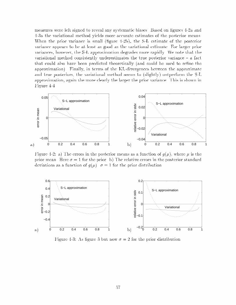
measures were left signed to reveal any systematic biases. Based on �gures 4-2a and4-3a the variational method yields more accurate estimates of the posterior means.When the prior variance is small (�gure 4-2b), the S-L estimate of the posteriorvariance appears to be at least as good as the variational estimate. For larger priorvariances, however, the S-L approximation degrades more rapidly. We note that thevariational method consistently underestimates the true posterior variance { a factthat could also have been predicted theoretically (and could be used to re�ne theapproximation). Finally, in terms of the KL-divergences between the approximateand true posteriors, the variational method seems to (slightly) outperform the S-Lapproximation, again the more clearly the larger the prior variance. This is shown inFigure 4-4.a) 0 0.2 0.4 0.6 0.8 1

−0.05

0

0.05

erro

r in

mea

n

S−L approximation

Variational b) 0 0.2 0.4 0.6 0.8 1

−0.04

−0.02

0

0.02

0.04

rela

tive

erro

r in

std

v S−L approximation

VariationalFigure 4-2: a) The errors in the posterior means as a function of g(�), where � is theprior mean. Here � = 1 for the prior. b) The relative errors in the posterior standarddeviations as a function of g(�). � = 1 for the prior distribution.a) 0 0.2 0.4 0.6 0.8 1

−0.4

−0.2

0

0.2

0.4

0.6

erro

r in

mea

n

S−L approximation

Variational b) 0 0.2 0.4 0.6 0.8 1−0.2

−0.1

0

0.1

0.2

rela

tive

erro

r in

std

v S−L approximation

VariationalFigure 4-3: As �gure 3 but now � = 2 for the prior distribution.57

a) 0 0.2 0.4 0.6 0.8 10

0.5

1

1.5

2

2.5

KL−

dive

rgen

ce S−L approximation

Variational b) 0 0.2 0.4 0.6 0.8 10

0.5

1

1.5

2

2.5

KL−

dive

rgen

ce S−L approximation

VariationalFigure 4-4: KL-divergences between the approximate and the true posterior distribu-tion as a function of g(�). a) � = 2 for the prior. b) � = 3. The two approximationmethods have (visually) identical curves for � = 1.4.5 Extension to belief networksA belief network can be constructed from logistic regression models that de�ne condi-tional probabilities of a variable given its parents3. The predictive joint distributionfor this belief network takes the usual product formP (S1; : : : ; Sn) =Yi P (SijSpai) (4.13)where Spai is the set of parents of Si. We note that this is an extension of sigmoidbelief networks (Neal 1992) due to the prior distributions over the parameters. Inorder to be able to use the techniques we have described for computing the poste-rior distributions on parameters in this setting, we assume �rst that the observationsare complete, i.e., contain a value assignment for all the variables in the network.Complete observations contain all the Markov blankets4 for the parameter distribu-tions de�ning the conditional models (see �gure 4-5a). Given value assignments forthe variables in the Markov blanket, i.e., for the variables in the associated con-ditional model, the parameter distributions become independent of everything elsein the network. Consequently, the posterior distributions over the parameters foreach conditional model remain independent from each other as well. To estimate theparameters distributions based on complete observations therefore reduces to n inde-pendent subproblems of estimating each of the conditional regression models, whichcan be done as before.4.5.1 Incomplete cases3The sets of parents for the variables must be consistent with some global ordering of the variables.4Markov blanket for a variable consists of any set of variables such that, conditionally on thevariables in the Markov blanket, the variable in question becomes independent from the remainingvariables in the probability model. 58

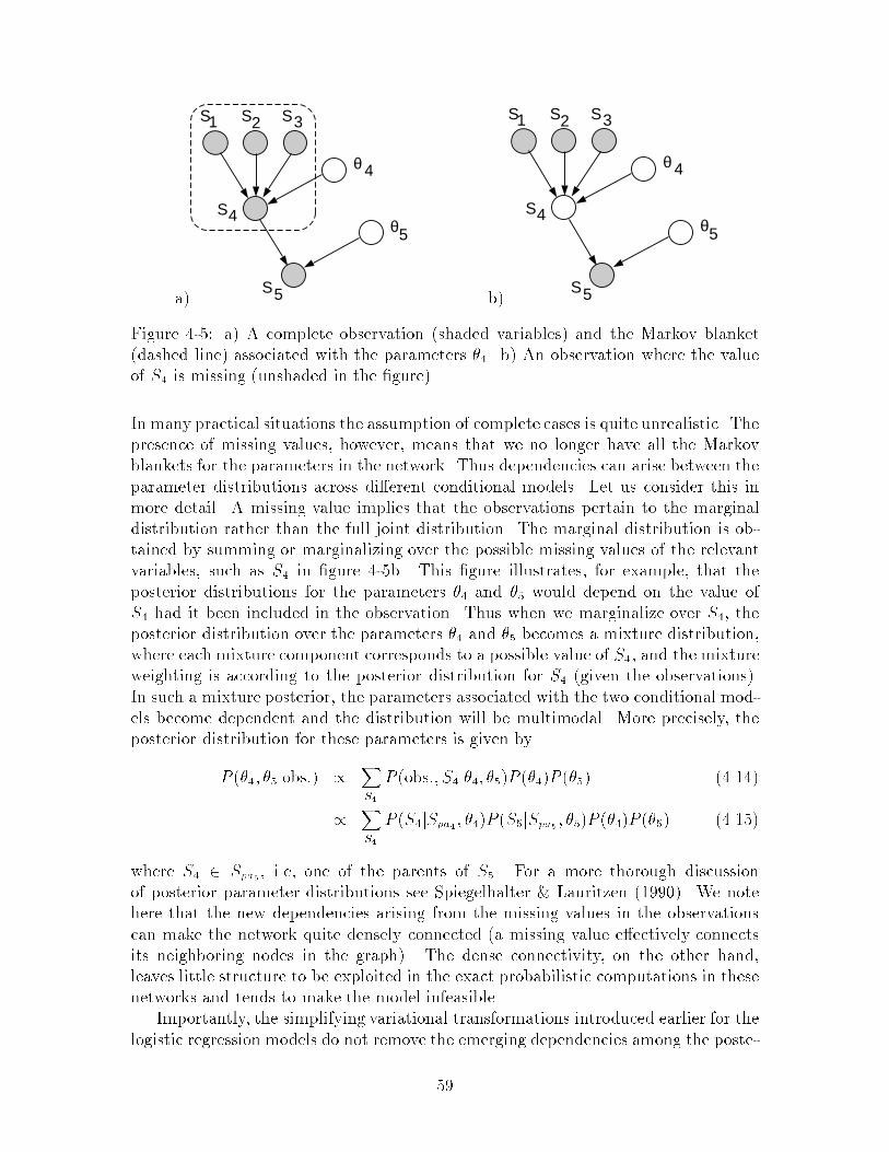
a)2S 3S1S

θ 4

S4

S5

θ5 b)2S 3S1S

θ 4

S4

S5

θ5Figure 4-5: a) A complete observation (shaded variables) and the Markov blanket(dashed line) associated with the parameters �4. b) An observation where the valueof S4 is missing (unshaded in the �gure).In many practical situations the assumption of complete cases is quite unrealistic. Thepresence of missing values, however, means that we no longer have all the Markovblankets for the parameters in the network. Thus dependencies can arise between theparameter distributions across di�erent conditional models. Let us consider this inmore detail. A missing value implies that the observations pertain to the marginaldistribution rather than the full joint distribution. The marginal distribution is ob-tained by summing or marginalizing over the possible missing values of the relevantvariables, such as S4 in �gure 4-5b. This �gure illustrates, for example, that theposterior distributions for the parameters �4 and �5 would depend on the value ofS4 had it been included in the observation. Thus when we marginalize over S4, theposterior distribution over the parameters �4 and �5 becomes a mixture distribution,where each mixture component corresponds to a possible value of S4, and the mixtureweighting is according to the posterior distribution for S4 (given the observations).In such a mixture posterior, the parameters associated with the two conditional mod-els become dependent and the distribution will be multimodal. More precisely, theposterior distribution for these parameters is given byP (�4; �5jobs:) / XS4 P (obs:; S4j�4; �5)P (�4)P (�5) (4.14)/ XS4 P (S4jSpa4; �4)P (S5jSpa5; �5)P (�4)P (�5) (4.15)where S4 2 Spa5, i.e, one of the parents of S5. For a more thorough discussionof posterior parameter distributions see Spiegelhalter & Lauritzen (1990). We notehere that the new dependencies arising from the missing values in the observationscan make the network quite densely connected (a missing value e�ectively connectsits neighboring nodes in the graph). The dense connectivity, on the other hand,leaves little structure to be exploited in the exact probabilistic computations in thesenetworks and tends to make the model infeasible.Importantly, the simplifying variational transformations introduced earlier for thelogistic regression models do not remove the emerging dependencies among the poste-59

rior parameter distributions. Thus unlike in the regression case, where the posteriorparameter distributions remained simple Gaussians, the use of these variational trans-formations with missing values yields not a single Gaussian posterior but a (large)mixture of them containing parameter distributions for other conditional models aswell. To avoid such connectivity and multimodality, further approximations are nec-essary. What should the nature of these approximations be? Ideally, we would liketo return to the setting of complete observations, where the parameter distributionscan be maintained locally. Such a transition, however, would presume having \�lled-in" the missing values. We propose to perform this �ll-in in a principled manner byresorting to an additional variational technique known as the mean �eld transforma-tion.In the context of belief networks, mean �eld transformation can be characterizedas a form of relaxed marginalization. The correct marginalization is a global operationin the sense that it a�ects synchronously all the conditional models that depend on thevariable being marginalized over. Mean �eld, on the other hand, is a local operationby acting individually on the relevant conditional models. In other words, mean�eld approximation simply transforms separately all the conditional models in thebelief network that pertain to the marginalized variable. Importantly, this localitypreserves the factorization of the joint distribution as with complete observationsthus performing the desired \�lled-in" of the missing value. More precisely, thetransformation of the (relevant) conditional models is given byP (SjSpa; �)!YS0 P (SjSpa; �)q(S0) (4.16)where S 0 is the variable with a missing value assignment and q(S 0) is a mean �elddistribution over the missing values. The variational parameter in this transformationis the distribution q. The transformed conditional probabilities are thus geometricallyaveraged over the missing values (with respect to the mean �eld distribution). Notethat if the particular conditional probability does not depend on the missing value theabove transformation will not change it. While the transformations are carried outseparately for each relevant conditional model, the mean �eld distribution associatedwith any particular missing value remains the same across such transformations. Wenote that the transformation does include a multiplicative constant that depends onq (see Appendix 4.B for more details).The use of mean �eld with in maintaining the Bayesian parameter distributionsis straightforward. When absorbing evidence from observations with missing val-ues we �rst apply the mean �eld transformation to �ll-in the missing values. Theresulting joint distribution factorizes as with complete observations but now con-tains transformed conditional probabilities. The posterior parameter distributionstherefore can be obtained independently for the parameters associated with di�erent(transformed) conditionals. Two issues remain to be considered. First, the trans-formed conditional probabilities are now products of logistic functions and thereforemore complicated than before. The introduction of the variational transformationsfor the logistic functions, however, turns them into exponentials with quadratic de-60

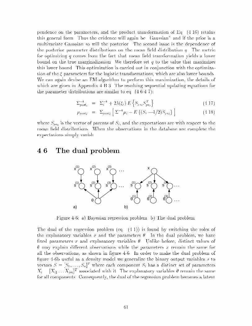
pendence on the parameters, and the product transformation of Eq. (4.16) retainsthis general form. Thus the evidence will again be \Gaussian" and if the prior is amultivariate Gaussian so will the posterior. The second issue is the dependence ofthe posterior parameter distributions on the mean �eld distribution q. The metricfor optimizing q comes from the fact that mean �eld transformation yields a lowerbound on the true marginalization. We therefore set q to the value that maximizesthis lower bound. This optimization is carried out in conjunction with the optimiza-tion of the � parameters for the logistic transformations, which are also lower bounds.We can again devise an EM-algorithm to perform this maximization, the details ofwhich are given in Appendix 4.B.3. The resulting sequential updating equations forthe parameter distributions are similar to eq. (4.6-4.7):��1posti = ��1i + 2�(�i) E nSpaiSTpaio (4.17)�posti = �posti h ��1�i + E f(Si � 1=2)Spaig i (4.18)where Spai is the vector of parents of Si, and the expectations are with respect to themean �eld distributions. When the observations in the database are complete theexpectations simply vanish.4.6 The dual problem. . .

. . .

θ

s s s(1) (2) (3)

x x x(1) (2) (3)

. . .

. . .s s s(1) (2) (3)

x

(1) (2) (3)θ θ θ

a) b)Figure 4-6: a) Bayesian regression problem. b) The dual problem.The dual of the regression problem (eq. (4.1)) is found by switching the roles ofthe explanatory variables x and the parameters �. In the dual problem, we have�xed parameters x and explanatory variables �. Unlike before, distinct values of� may explain di�erent observations while the parameters x remain the same forall the observations, as shown in �gure 4-6. In order to make the dual problem of�gure 4-6b useful as a density model we generalize the binary output variables s tovectors S = [S1; : : : ; Sn]T where each component Si has a distinct set of parametersXi = [Xi1 : : :Xim]T associated with it. The explanatory variables � remain the samefor all components. Consequently, the dual of the regression problem becomes a latent61

variable density model with a joint distribution given byP (S1; : : : ; SnjX) = Z "Yi P (SijXi; �)#P (�)d� (4:19)where the conditional probabilities are logistic regression modelsP (SijXi; �) = g �(2Si � 1)PjXij�j� (4:20)We would like to use the EM- algorithm for parameter estimation in this latentvariable density model. To achieve this, we again make use of the variational trans-formations. These transformations are introduced for each of the conditional proba-bilities in the above joint distribution and optimized separately for the observationsDt = fSt1; : : : ; Stng in the database (note that the observations now consist of only thevalues for the binary output variables). As in the logistic regression case, the trans-formations change the unwieldy conditional models into simpler ones that depend onthe parameters only quadratically in the exponent (they become \Gaussian"). Thevariational evidence, which is a product of the transformed conditional probabilities,retains the same property. We are thus able to obtain the posterior distribution cor-responding to such \Gaussian" evidence and, analogously to the regression case, themean and the covariance of this posterior are given by��1t = ��1 +Xi 2�(�ti )XiXTi (4.21)�t = �t "��1� +Xi (Sti � 1=2)Xi# (4.22)The variational parameters �ti associated with each observation and the conditionalmodel can be updated using eq. (4.8) assuming Xpa is replaced with Xi, the vectorof parameters associated with the ith conditional model. After we have computedthe posterior distributions for all the observations in the data set, we can solve theM-step exactly. Omitting the algebra we get the following updates� 1T Xt �t (4.23)� 1T Xt �t (4.24)Xi A�1i bi (4.25)where Ai = Xt 2�(�ti ) (�t + �t�Tt ) (4.26)bi = Xt (Sti � 1=2)�t (4.27)We note �nally that since the variational transformations are lower bounds, these62

updates result in a monotonically increasing lower bound on the log-likelihood of theobservations. This desirable monotonicity property is unlikely to arise with othertypes of approximation methods, such as the Laplace approximation.4.7 Technical note: ML estimationThe standard maximum likelihood procedure for estimating the parameters in logisticregression uses an iterative Newton-Raphson method to �nd the parameter values.While the method is fast, it is not monotonic; i.e., the likelihood of the observationsis not guaranteed to increase after an iteration. We show here how to derived amonotonic, fast estimation procedure for logistic regression by making use of thevariational transformation in eq. (4.4). Let us denote Ht = (2St � 1)Pj �jX tj andwrite the log-likelihood of the observations asL(�) =Xt logP (StjX t; �) =Xt log g(Ht)� Xt log g(�t) + (Ht � �t)=2� �(�t) �H2t � �2t �= L(�; �) (4.28)The variational lower bound is exact whenever �t = Ht for all t. Although theparameters � cannot be solved easily from L(�), L(�; �) allows a closed form solutionfor any �xed �, since the variational log-likelihood is a quadratic function of �. Theparameters � that maximize L(�; �) are given by �0 = A�1b whereA =Xt 2�(�t)HtHtT and b =Xt (St � 1=2)Ht (4:29)Successively solving for � and updating � yields the following chain of inequalities:L(�) = L(�; �) � L(�0; �) � L(�0; �0) = L(�0) (4:30)where the prime signi�es an update and we have assumed that �t = Ht initially. Thecombined update thus leads to a monotonically increasing likelihood. In addition,the closed form �-updates make this procedure comparable in speed to the standardNewton-Raphson alternative.4.8 DiscussionWe have exempli�ed the use of variational techniques in a Bayesian estimation prob-lem. We found that variational methods can be employed to obtain closed formexpressions that approximate the posterior distributions for the parameters in lo-gistic regression and associated belief networks even in the case of missing values.Furthermore, our variational techniques lead to an exactly solvable EM algorithm fora type of latent variable density model|the dual of the regression problem.63

ReferencesJ. Bernardo and A. Smith (1994). Bayesian theory. New York: Wiley.D. Heckerman, D. Geiger, and D. Chickering (1995). Learning Bayesian networks:the combination of knowledge and statistical data. Machine Learning 20 No. 3: 197.J. Hertz, A. Krogh and R. Palmer (1991). Introduction to the theory of neural com-putation. Addison-Wesley.P. McCullagh & J. A. Nelder (1983). Generalized linear models. London: Chapmanand Hall.R. Neal (1992). Connectionist learning of belief networks. Arti�cial Intelligence 56:71-113.R. Neal (1993). Probabilistic inference using Markov chain Monte Carlo methods.Technical report CRG-TR-93-1, University of Toronto.G. Parisi (1988). Statistical �eld theory. Addison-Wesley.D. Spiegelhalter and S. Lauritzen (1990). Sequential updating of conditional proba-bilities on directed graphical structures. Networks 20: 579-605.4.A Optimization of the variational parametersTo optimize the variational approximation of eq. (4.5) in the context of an observationD = fS;X1; : : : ;Xng we formulate an EM algorithm to maximize the predictivelikelihood of this observation with respect to �. In other words, we �nd � thatmaximizes the right hand side ofZ P (SjX; �)P (�)d� � Z P (SjX; �; �)P (�)d� (4:31)In the EM formalism this is achieved by iteratively maximizing the expected completelog-likelihood given by Q(�j�old) = E flogP (SjX; �; �)P (�)g (4:32)where the expectation is over P (�jD; �old). Taking the derivative of Q with respectto � and setting it to zero leads to@@�Q(�j�old) = �@�(�)@� 24E (Xj �jXj)2 � �235 = 0 (4:33)64

As �(�) is a monotonically decreasing function5 the maximum is obtained at�2 = E (Xj �jXj)2 (4:34)By substituting � for �old above, the procedure can be repeated. Each such iterationyields a better approximation in the sense of eq. (4.31).4.B Parameter posteriors through mean �eldHere we consider in detail the use of mean �eld in �lling-in the missing values to facil-itate the computation of posterior parameter distributions. We start by introducingthe mean �eld approximation from the point of view that will be most convenient forour purposes. We note that several di�erent formulations exist for mean �eld (Parisi1988); the one presented here is tailored for our purposes.4.B.1 Mean �eldAs mentioned in the text, mean �eld can be viewed as an approximation to marginal-ization. Consider therefore the problem of marginalizing over the variable S 0 whenthe joint distribution is given byP (S1; : : : ; Snj�) =Yi P (SijSpai; �i) (4.35)If we performed the marginalization exactly, then the resulting distribution would notretain the same factorization as the original joint (assuming S 0 is involved in morethan one of the conditionals then) as can be seen fromXS0 Yi P (SijSpai; �i) = "Yi00 P (SijSpai; �i)#XS0 Yi0 P (SijSpai; �i) (4.36)where we have partitioned the product over the conditionals according to whetherthey depend on S 0 (indexed by i0) or not (indexed by i00). Marginalization is thereforenot a local operation. Locality is a desirable property for computational reasons,however, and we attempt to preserve locality under approximate marginalization.The approximation we use for this purpose is a variational transformation based onthe fact that any geometric average6 is always less than or equal to the usual average.By applying this property to the marginalization, we �ndXS0 P (S1; : : : ; Snj�) = XS0 q(S 0) "P (S1; : : : ; Snj�)q(S 0) # (4.37)5This holds for � � 0. However, since P (SjX; �; �) is a symmetric function of �, assuming � � 0has no e�ect on the quality of the approximation.6A geometric average over xi; i 2 f1; : : : ; ng with respect to the distribution qi is given byQi xqii .65

� YS0 "P (S1; : : : ; Snj�)q(S 0) #q(S0) (4.38)= C(q)Yi "YS0 P (SijSpai; �i)q(S0)# (4.39)where the inequality comes from transforming the average over the bracketed term(with respect to the distribution q) into a geometric average. The third line followsfrom plugging in the form of the joint distribution and exchanging the order of theproducts. The multiplicative constant C(q) relates to the entropy of the variationaldistribution qC(q) =YS0 " 1q(S 0)#q(S0) and therefore logC(q) = �XS0 q(S 0) log q(S 0) (4.40)Let us now make a few observations about the result in Eq. (4.39). First, the choiceof the variational distribution q always involves a trade-o� between feasibility andaccuracy. For example, if q were chosen to be the posterior distribution for S 0 giventhe remaining variables in the network, then the transformation would be exact ratherthan a lower bound. While attaining perfect accuracy, this choice would amount to nosimpli�cation. We emphasize feasibility and consequently assume that the variationaldistribution q depends only on the variable being marginalized over (i.e., S 0). Theresulting lower bound is the mean �eld approximation. Second, for any �xed q and formean �eld in particular, the transformed marginalization (in Eq. (4.39)) follows thefactorization of the original joint distribution. The conditional probabilities, however,have been modi�ed in this approximation (mean �eld) according toP (SijSpai; �i)!YS0 P (SijSpai; �i)q(S0) (4.41)Unlike correct marginalization, this transformation of conditional probabilities is alocal operation. Note that the transformation has no e�ect on the conditional prob-abilities that do not depend on S 0. We note that the mean �eld distribution q is thesame in all transformations corresponding to the same missing value.Let us lastly explicate the case where the missing variable S 0 is in fact a set ofvariables, i.e., S 0 = fS 01; : : : ; S 0mg. It might not be feasible in this case to allow thevariational distribution q to vary independently for each con�guration of the variablesin S 0; nor would it be a mean �eld approximation. Indeed, mean �eld approximationin this case would consist of successive applications of the conditional transformationsfor each of the variables in S 0. It can be easily veri�ed that this is equivalent totransforming the conditional probabilities for the whole set S 0 using a product orfactorized distribution q(S 0) = mYi=1 qi(S 0i) (4.42)66

4.B.2 Parameter posteriorsTo �ll-in the missing values in an observation Dt = fsti; : : :g we use the mean �eldapproximation. As a result, the joint distribution factorizes as with complete ob-servations. Thus the posterior distributions for the parameters remain independentacross the di�erent conditional models and can be computed separately. Accordingly,P (�ijDt; q) / "YS0 P (SijSpai; �i)q(S0)#P (�i) (4.43)Even with the mean �eld approximation, however, this posterior remains at least asunwieldy as the Bayesian logistic regression problem considered earlier. Similarly tothat case, we introduce the logistic transformations from Eq. (4.4) for the conditionalprobabilities and obtainP (�ijDt; q; �) / " YS0 P (SijSpai; �i; �i)q(S0) # P (�i) (4.44)= " YS0 n g(�) e(HSi��)=2��(�)(H2Si��2) oq(S0) # P (�i) (4.45)= "g(�) ePS0 q(S0)n (HSi��)=2��(�)(H2Si��2)o # P (�i) (4.46)= hg(�) e (EfHSig�� )=2��(�)(EfH2Sig��2 ) i P (�i) (4.47)� P (SijSpai; �i; �i; q)P (�i) (4.48)where HSi = (2Si�1)�Ti Spai, and Spai is the vector of parents of Si. The expectationsare with respect to the mean �eld distribution q and, for simplicity, we have used thesame variational parameter � for all the conditionals involved. The latter is naturallysuboptimal but may be necessary if the number of missing values is large. Now, sinceHSi is linear in the parameters �i, the exponent in Eq. (4.47), consisting of averagesover HSi and its square, stays at most quadratic in the parameters �i. This propertyimplies that if the prior distribution is a multivariate Gaussian so will the posterior.The mean �posti and covariance �posti of such posterior are given by (we omit thealgebra) ��1posti = ��1i + 2�(�i) E nSpaiSTpaio (4.49)�posti = �posti h ��1i �i + E f(Si � 1=2)Spaig i (4.50)The expectations here are with respect to the mean �eld distribution q. Note that thisposterior depends both on the distribution q and the parameters �. The optimizationof these parameters is shown in Appendix 4.B.3.67

4.B.3 Optimization of the variational parametersWe have introduced two variational \parameters": the mean �eld distribution q forthe missing values, and the � parameters corresponding to the logistic transforma-tions. The metric for optimizing the parameters comes from the fact that both ofthe transformations associated with these parameters introduce a lower bound onthe likelihood of the observations. Thus by maximizing this lower bound we �nd theparameter values that yield the most accurate approximations. We therefore attemptto maximize the right hand side oflogP (Dt) � log P (Dtj�; q) (4.51)= log Z P (Dtj�; �; q)P (�)d� (4.52)= logYi Z P (SijSpai; �i; �i; q)P (�i)d�i + logC(q) (4.53)where Dt is contains the observed variable settings. We have used the fact that thejoint distribution in our approximation factorizes as with complete cases. Similarlyto the case of Bayesian logistic regression considered previously, we can devise anEM-algorithm to maximize the variational log-likelihood of observations with respectto the parameters q and �; the parameters � are considered as latent variables in thisformulation. The E-step of the EM-algorithm, i.e., �nding the posterior distributionover the latent variables, has already been described in Appendix 4.B.2. Here we willconsider in detail only the M-step. For simplicity, we solve the M-step in two phases:one where the mean �eld distribution is kept �xed and the maximization is over �,and the other where these roles have been reversed. We start with the �rst phase.As the variational joint distribution factorizes, the problem of �nding the optimal� parameters separates into independent problems concerning each of the transformedconditional. Thus the optimization becomes analogous to the simple Bayesian logisticregression considered earlier. Two di�erences exist: �rst, the posterior over each �iis now obtained from Eq. (4.48); second, we have an additional expectation withrespect to the mean �eld distribution q. As to the second di�erence, we note that themean �eld expectations appear only in the exponents of the transformed conditionals(see Eq. (4.48) above). The signi�cance of this feature lies in the fact that suchexpectations can always be incorporated into the E-step simply as additional averages.Reinterpreting the E-step in this manner reduces the problem to the simple regressionexplained earlier. For this reason we don't repeat the resulting EM-algorithm ofAppendix 4.A here.The latter part of our two-stage M-step is new, however, and will be consideredin detail. The purpose here is to hold the parameters � �xed and instead optimizeover q. In this case we do not include the mean �eld averages into the E-step, butmore traditionally computeQ(qjqold) = EflogP (Dt; �j�; q)g (4.54)= Xi Ei flog P (SijSpai; �i; �i; q)P (�i)g+ logC(q) (4.55)68

where the �rst expectation is with respect to P (�j�; qold), which factorizes acrossthe conditional models as explained previously; the expectations Ei are over thecomponents P (�ij�i; qold), obtained directly from Eq. (4.48). Let us now insert theform of the transformed conditional probabilities, P (SijSpai; �i; �i; q), into the abovede�nition of the Q function. For clarity we will omit all the terms that have nodependence on the mean �eld distribution q as they will be irrelevant to our M-step.After some algebra we obtain:Q(qjqold) = Xi Ei n EqfHSig=2 � �(�i)EqfH2Sig o+ logC(q) + : : : (4.56)= Eq Xi n EifHSig=2 � �(�i)EifH2Sig o+H(q) + : : : (4.57)where Eq refers to the expectation with respect to the mean �eld distribution q. Thesecond equation follows by exchanging the order of the expectations Ei and Eq, whichare mutually independent. We have also used the fact that logC(q) is the entropyH(q) of the mean �eld distribution q (see Appendix 4.B above). Recall the notationHSi = (2Si�1)�Ti Spai, where Spai is a binary vector of parents of Si. Before proceedingto maximize the Q function with respect to q, we explicate the averages Ei in theabove formula: EifHSig = (2Si � 1)�TpostiSpai (4.58)EifH2Sig = ��TpostiSpai�2 + STpai�postiSpai (4.59)Here �posti and �posti are the mean and the covariance, respectively, of the posteriorP (�ij�i; qold) for the parameters of the ith conditional model. Simply putting theseback into the expression for the Q function we getQ(qjqold) = EqXi � (2Si � 1)�TpostiSpai=2 � �(�i) ��TpostiSpai�2��(�i) STpai�postiSpai o+H(q) + : : : (4.60)Now, some of the binary variables s have a value assignment based on the observationDt and the remaining variables will be averaged over the mean �eld distribution q. Areader familiar with Boltzmann machines will notice that since the binary variablesappear only quadratically in the above formula, the Q function can be viewed asa mean �eld approximation for a type of Boltzmann machine (see e.g., Hertz et al.1991). The (locally) maximizing distribution q can therefore be obtained throughsequentially solving @@qkQ(qjqold) = 0 (4.61)for each of the component distributions (here qk = qk(Sk = 1)). The solutions forthese can be found in closed form and each update leads to a monotonically increasingQ(qjqold). The latter property follows from the fact Q(qjqold) is a concave function69

of each of the component distributions (the expectation is linear and the entropyconcave) implying a single attainable maximum. Note that the concavity propertydoes not necessarily hold globally since the mean �eld expectations over the quadraticterms yield bi-linear forms with respect to these component distributions; we may nottherefore be able to obtain the globally optimal mean �eld distribution.

70

Chapter 5Variational methods in medicaldiagnosis5.1 IntroductionThe wealth and complexity of information in modern medicine underlies the tendencytowards automated processing. In addition to low level processing aids, automatedtechniques can serve as powerful tools in more cognitive tasks such as in diagnosis.An example of such diagnostic tool, and the one considered in this chapter, is theQuickMedical Reference (QMR) knowledge base, compiled for internal medicine. Theknowledge base embeds a combination of statistical and expert knowledge of about600 signi�cant diseases and their associated �ndings (about 4000). The intended useof this knowledge base is as an interactive decision tool for a practicing doctor ininternal medicine. For the purpose of diagnosis, an early version of QMR includeda heuristic reasoning mechanism for suggesting underlying diseases based on known�ndings (laboratory results or physicians' observations), or to outline informativetests to be carried out in order to verify a disease hypothesis, among other things.The reliance of heuristic tools for diagnostic reasoning, however, leaves much to bedesired. The employed reasoning methods, for example, may be inconsistent and theycan hide the assumptions underlying the success or failure of obtained diagnoses.QMR-DT (Shwe et al. 1991), a decision theoretic reformulation of the QMRknowledge base, provides a more rigorous basis for automated inference. The rela-tionships between the diseases and �ndings in this formulation take the form of abelief network (see e.g. Pearl 1988, Jensen 1996). Such probabilistic format enhancesinterpretability by allowing relevant assumptions to be explicated and, furthermore,endows the system with consistent rules of inference that are readily available fordiagnostic (and other) decision making. The semantic rigor brought by the use ofprobability theory, however, often comes with a sizable computational cost of evalu-ating the conclusion implied by the probabilistic framework. Probabilistic inference,after all, has been shown to be an NP-hard problem in general (Cooper 1990). Thesize and complexity of the QMR belief network in particular appears to render exactevaluation methods inapplicable. To reap the bene�ts from the probabilistic formula-tion of the QMR network, we are forced to consider approximate methods for carrying71

out the inferences.Several objectives can be set for approximate methods replacing exact calculations.Such methods �rst of all should be consistent in that, given enough computationalresources, they would yield the result implied by the probabilistic model. Second,we should be able to assess the reliability of the results when such computationalresources are not available. In the context of the QMR-belief network, Shwe et al.(1991) (see also Shwe & Cooper 1991) proposed the use of sampling techniques toobtain estimates of the posterior probabilities for the diseases (diagnoses in proba-bilistic terms). Sampling methods meet the �rst of our objectives since, in the limitof a large number of samples, the estimates will converge to the correct ones undermild conditions. The second objective, however, remains largely unattained by thesetechniques.In this chapter we apply and extend an alternative approximation framework,that of variational methods, to compute the posterior probabilities for the diseases inthe QMR belief network. Variational methods have a long history as approximationtechniques in the physics literature. Unlike sampling methods variational techniquesyield deterministic approximations that are adapted to each case separately. We con-sider here a particular type of variational methods, those most applicable to the QMRbelief network. These techniques can be readily merged with exact evaluation meth-ods in the QMR setting and therefore allowing us to let the available computationalresources to determine the extent to which approximations are introduced. Towardsthe second objective for approximate methods, the variational methods yield explicitexpressions for the posterior probabilities of the diseases. These expressions in turncan be subjected to further analysis concerning the accuracy and sensitivity to thevarious aspects of each case under consideration.We start by de�ning the QMR belief network and the inference problem we aretrying to solve through the use of variational methods. We then introduce and developthe variational techniques used in the chapter. Finally, we report numerical resultson the accuracy and usefulness of variational techniques in diagnostic reasoning.5.2 The QMR-DT belief networkThe structure of the QMR-DT belief network currently conforms to the class of two-level or bi-partite networks (see �gure 5-1). The diseases and �ndings in this modeloccupy the nodes on the two levels of the network, respectively, and the conditionalprobabilities specifying the dependencies between the levels are assumed to be noisy-OR gates. The bi-partite network structure encodes the assumption that, in theabsence of �ndings, the diseases appear independently from each other with theirrespective prior probabilities (i.e. marginal independence). Also evident from thestructure is that conditionally on the states of the diseases the �ndings are inde-pendent of each other (conditional independence). For a more thorough discussionregarding the medical validity of these and other assumptions embedded into theQMR-DT belief network, we refer the reader to Shwe et al. (1991).To state more precisely the probability model implied by the QMR-DT belief72

...

...

Diseases

Findings

d 1 d n

f 1 f2Figure 5-1: The QMR belief network is a two-level network where the dependenciesbetween the diseases and their associated �ndings have been modeled via noisy-ORgates.network, we write the joint probability of diseases and �ndings asP (f; d) = P (f jd)P (d) = "Yi P (fijd)# 24Yj P (dj)35 (5.1)where d and f are binary (1/0) vectors referring to presence/absence states of thediseases and the positive/negative states or outcomes of the �ndings, respectively.The conditional probabilities P (fijd) for the �ndings given the states of the diseases,are assumed to be a noisy-OR models:P (fi = 0jd) = P (fi = 0jL) Yj2pai P (fi = 0jdj) (5.2)= (1� qi0) Yj2pai(1 � qij)dj = e��i0�Pj2pai �ijdj (5.3)Here pai (\parents" of i) is the set of diseases pertaining to �nding fi. qij = P (fi =0jdj = 1) is the probability that the disease j, if present, could alone cause the �ndingto have a positive outcome (i.e. 1). qi0 = P (fi = 0jL) is the \leak" probability, i.e.,the probability that the �nding is caused by means other than the diseases includedin the belief network model. The noisy-OR probability model encodes the causalindependence assumption (Shwe et al., 1991), i.e., that the diseases act independentlyto cause the outcome of the �ndings. The exponentiated notation with �ij = � log(1�qij) will be used later in the chapter for reasons of clarity.5.3 InferenceTo carry out diagnostic inferences in the QMR belief network involves computingposterior (marginal) probabilities for the diseases given a set of observed positive(fi = 1) and negative (fi0 = 0) �ndings. Note that these sets are considerably smaller73

than the set of possible �ndings; the posterior probabilities for the diseases are a�ectedonly by �ndings whose states we have observed. For brevity we adopt the notationwhere f+i corresponds to the event fi = 1, and similarly f�i refers to fi = 0 (positiveand negative �ndings respectively). Thus the posterior probabilities of interest areP (dj jf+; f�), where f+ and f� are the vectors of positive and negative �ndings. Thecomputation of these posterior probabilities exactly is in the worst case exponentiallycostly in the number of positive �ndings (Heckerman, 1988; D'Ambrosio 1994); thenegative �ndings f�, on the other hand, can be incorporated in linear time (in thenumber of associated diseases and in the number of negative �ndings). In practicaldiagnostic situations the number of positive �ndings often exceeds the feasible limitfor exact calculations.Let us consider the inference calculations more speci�cally. To �nd the posteriorprobability P (djf+; f�), we �rst absorb the evidence from negative �ndings, i.e.,compute P (djf�). This is just P (f�jd)P (d) with normalization. Since both P (f�jd)and P (d) factorize over the diseases (see Eq. (5.2) and Eq. (5.1) above), the posteriorP (djf�) must factorize as well. The normalization of P (f�jd)P (d) therefore reducesto independent normalizations over each disease and can be carried out in time linearin the number of diseases (or negative �ndings). In the remainder, we will concentratesolely on the positive �ndings as they pose the real computational challenge. Unlessotherwise stated, we will assume that the prior distribution over the diseases alreadycontains the evidence from the negative �ndings. In other words, we presume thatthe updates P (dj) P (dj jf�) have already been made.We now turn to the question about how to compute P (dj jf+), the posteriormarginal probability based on the positive �ndings. Formally, to obtain such a pos-terior involves marginalizing P (f+jd)P (d) over all the remaining diseases, i.e.P (dj jf+) / Xdndj P (f+jd)P (d) (5.4)In the QMR belief network P (f+jd)P (d) has the formP (f+jd)P (d) = "Yi P (f+i jd)# 24Yj P (dj)35 = "Yi �1� e��i0�Pj �ijdj�# 24Yj P (dj)35(5.5)which follows from the notation in Eq. (5.3) and the fact that P (f+i jd) = 1 �P (f�jd). To perform the summation in Eq. (5.4) over the diseases, we would haveto multiply out the terms 1 � ef�g corresponding to the conditional probabilities foreach positive �nding. The number of resulting terms would be exponential in thenumber of positive �ndings and is not feasible. There is, however, local structure inthe dependencies in the QMR belief network that can be exploited to speed up thecomputation (D'Ambrosio, 1994). For example, some �ndings are associated withonly a few diseases. The gain from exploiting the local structure nevertheless doesnot appear to be su�cient to render the inference problem tractable in a practicalsetting. 74

5.4 Variational methods5.4.1 A brief introductionThe variational approximation techniques we use and extend in this chapter are basedon those developed in chapter 2 for noisy-OR networks. The extension considered inthe current chapter pertains to the integration of these methods with exact probabilis-tic calculations rather than to the transformations themselves. For readers unfamiliarwith the results of chapter 2 we have included a brief introductory presentation below.Other readers may wish to skip this material and commence from around Eq. (5.13).The objective of our approximation methods is to simplify a complicated jointdistribution such as the one in Eq. (5.5) above through variational transformations ofconditional probabilities. The transformations themselves rerepresent the conditionalprobabilities in terms of optimization problems. Such representations are naturallyturned into approximations by relaxing the optimizations involved. The fact thatthese approximations come from optimization problems implies that they have aninherent error metric associated with them, which is quite uncharacteristic of otherdeterministic or stochastic approximation methods. The use of this metric is toallow the approximation to be readjusted once they have been used, for example, incomputation of marginal probabilities.For the origin of the variational methods considered here we refer the reader tothe introductory section 1.1 of chapter 1. For the purposes of this chapter, we recallthat these methods transform any concave function f into an optimization problemby f(x) = min� f �Tx� f�(�) g (5.6)where f� is the dual or conjugate function and � is a variational parameter. If werelax the minimization above and �x the the variational parameter �, we obtain abound f(x) � �Tx� f�(�) (5.7)which is how the transformations are naturally used as approximations. We note thatthe reduction in complexity ensuing the substitution of the linear bound for f canbe huge. What is gained in simplicity may, however, be lost in accuracy but this isnot necessarily so. The loss in accuracy is contingent on the smoothness of f : thesmoother f is, the more accurate the bound is.5.4.2 Variational methods for QMRLet us now return to the problem of computing the posterior probabilities in theQMR belief network. Recall that it is the conditional probabilities corresponding to75

the positive �ndings that need to be simpli�ed. To this end, we writeP (f+i jd) = 1� e��i0�Pj �ijdj = e log(1�e�x) (5.8)where x = �i0 +Pj �ijdj. Consider the exponent f(x) = log(1 � e�x). For noisy-OR, as well as for many other conditional models involving compact representations(e.g. logistic regression), the exponent f(x) is a concave function of x. Based onthe introduction we know that there must exist a variational upper bound for thisfunction that is linear in x: f(x) � �x� f�(�) (5.9)The conjugate function f�(�) for noisy-OR is given by (see chapter 2 for a derivation)f�(�) = �� log � + (� + 1) log(� + 1) (5.10)The desired bound or simpli�cation of the noisy-OR conditional probabilities is foundby putting the above bound back into the exponent (and recalling the de�nitionx = �i0 +Pj �ijdj): P (f+i jd) = e f(x) (5.11)� e �i(�i0+Pj �ijdj)�f�(�i) (5.12)= e �i�i0�f�(�i)Yj he �i�ijidj (5.13)� P (f+i jd; �i) (5.14)where we have rewritten the bound as a product over the associated diseases tomake explicit the fact that it factorizes over such diseases. Importantly, any evidencepossessing this factorization can be absorbed e�ciently (in time and space) just aswith negative �ndings. Thus unlike the correct evidence P (f+i jd) from the positive�ndings, the \variational" evidence P (f+i jd; �i) can be incorporated e�ciently intothe posterior.We are now ready to outline the variational approximation framework for obtain-ing e�cient estimates of the posterior marginal probabilities for the diseases. The�rst step is to reduce the complexity of handling the positive �ndings by introducingthe transformations P (f+i jd)! P (f+i jd; �i) (5.15)Not all the positive �ndings need to be transformed, however, and we use thesetransformations only to the extent that is necessary to reduce the computational loadto a manageable (or practical) level. The posterior estimates can be consequentlyobtained from the transformed probability model.Two issues need to be clari�ed for this framework. The posterior estimates willdepend on the variational parameters � which we need to set and adjust to the76

current diagnostic context. This issue is resolved in Appendix 5.A; the adjustmentof the variational parameters reduces to convex optimization that can be carried oute�ciently (there are no local minima). The second issue is the question of whichconditional probabilities (or positive �ndings) should be transformed and which leftunchanged. This will be considered next.The order of transformationsThe decision to transform or treat exactly any of the conditional probabilities P (f+i jd)corresponding to the positive �ndings is a trade-o� between e�ciency and accuracy.To maintain a maximal level of accuracy while not sacri�cing e�ciency, we introducethe transformations by starting from the conditional for which the variational formis the most accurate and proceed towards less accurate transformations. When it ismanageable to treat the remaining conditionals exactly we stop introducing any fur-ther transformations. How then do we measure the accuracy of the transformations?The metric for this comes from the fact that the transformations are indeed bounds.Each transformation introduces an upper bound on the exact conditional prob-ability. Thus the likelihood of the observed (positive) �ndings P (f+) is also upperbounded by its variational counterpart P (f+j�):P (f+) =Xd P (f+jd)P (d) � Xd P (f+jd; �)P (d) = P (f+j�) (5.16)The better the variational approximations are, the tighter this bound is. We can assessthe accuracy of each variational transformation as follows. First we introduce andoptimize the variational transformations for all the positive �ndings. Then for eachpositive �nding we replace the variational transformation with the exact conditionaland compute the di�erence between the corresponding bounds on the likelihood ofthe observations: �i = P (f+j�) � P (f+j� n �i) (5.17)where P (f+j� n �i) is computed without transforming the ith positive �nding. Thelarger the di�erence � is, the worse the ith transformation is. We should thereforeintroduce the transformations in the ascending order of �s. Put another way, weshould treat exactly the �ndings for which � is large.Figure 5-2 illustrates the signi�cance of using the proposed ordering for introduc-ing the variational transformations as opposed to a random ordering. The two plotscorrespond to representative diagnostic cases, and show the log-likelihoods for theobserved �ndings as a function of the number of positive �ndings that were treatedexactly. We emphasize that the plots are on a log-scale and therefore the observeddi�erences are huge. We also note that the curves for the proposed ordering are con-vex, i.e., the bound improves the less the more �ndings have already been treatedexactly. This is because the exact conditionals �rst replace the worst transforma-tions and the di�erences among the better transformations are smaller. It is for thisreason that we can expect the variational posterior estimates to converge close to77

the true values after a reasonably small fraction of the positive �ndings have beentreated exactly. We �nally note that the � measure for determining the ordering fa-vors variational transformations for conditional probabilities that are diagnosticallythe least relevant. This is because the variational transformations are more accuratefor positive �ndings that are not surprising, i.e., are likely to occur, or when there isless impetus for explaining them (the leak probability is large). See Appendix 5.B fordetails.a) 0 2 4 6 8 10 12

−60

−55

−50

−45

−40

−35

−30

# of exactly treated findings

log−

likel

ihoo

d b) 0 2 4 6 8 10 12−75

−70

−65

−60

−55

−50

−45

# of exactly treated findings

log−

likel

ihoo

dFigure 5-2: The log-likelihood of the observed �ndings as a function of the number ofpositive �ndings treated exactly. The solid line corresponds to the proposed orderingand the dashed line is for a random ordering.5.5 Towards rigorous posterior boundsThe variational methods we have described earlier provide upper bounds on the likeli-hood of the observed �ndings. Other variational methods can be used to obtain lowerbounds on the same likelihoods. The ability to obtain upper and lower bounds onthe likelihoods provides the means for achieving such bounds on the desired posteriormarginals as well. To see why, note �rst that by Bayes' rule the posterior marginalscan be written in terms of likelihoods:P (dj = 1jf+) = P (dj = 1; f+)P (dj = 1; f+) + P (dj = 0; f+) (5.18)where, for example, P (dj = 1; f+) is the joint likelihood of the �ndings and thedisease j to be present. Let us assume that there are methods available for �ndinglikelihood bounds and use the notation P (�) for lower bounds and analogously P (�)for upper bounds. It follows from standard results (see e.g. Draper, 1994) that theposterior disease marginals in this case are bounded byP (dj = 1jf+) � P (dj = 1; f+)P (dj = 1; f+) + P (dj = 0; f+) (5.19)78

P (dj = 1jf+) � P (dj = 1; f+)P (dj = 1; f+) + P (dj = 0; f+) (5.20)Note that both upper and lower bounds are needed to obtain either an upper orlower bound on the posterior disease marginal. The techniques described in Jaakkola& Jordan (1996a) provide the missing lower bounds on the marginal likelihoods inthe QMR setting. While these methods can produce quite accurate lower boundsfor many networks, the speci�cs of the QMR belief network nevertheless precludestheir use. The reason for this discrepancy comes from the mathematical expansionsthat these lower bounds rely on: for very small leak probabilities such expansionsbecome unreliable. This is indeed the case with the QMR belief network whose leakprobabilities are typically quite small (can be as low as 10�7).We introduce here an alternative technique towards obtaining rigorous bounds onthe posterior marginals. Although we only use the upper bound variational technique,we make a more extensive use of its approximation properties. To this end, we adoptthe notation r(dj = 1; f+) to denote the ratio of the variational upper bound to thecorrect marginal likelihood, i.e.,r(dj = 1; f+) = P (dj = 1; f+)P (dj = 1; f+) (5.21)where r(dj = 0; f+) is de�ned analogously. We may now write the correct marginallikelihoods as P (dj = 1; f+)=r(dj = 1; f+). Substituting these for the correct likeli-hoods in Eq. (5.18) and multiplying by the ratio r(dj = 1; f+) givesP (dj = 1jf+) = P (dj = 1; f+)P (dj = 1; f+) + P (dj = 0; f+) r(dj=1;f+)r(dj=0;f+) (5.22)� P (dj = 1; f+)P (dj = 1; f+) + P (dj = 0; f+) (5.23)where the inequality follows from the conjecture (partially proved in Appendix 5.B)that the approximation in terms of the ratio is better for the case dj = 1. The keyhere is that the variational parameters are optimized individually to P (dj = 1; f+)and P (dj = 0; f+); otherwise, Eq. (5.23) would correspond exactly to the variationalposterior estimates discussed earlier and �gures 5-3 and 5-4 below would refute theconjecture in that regard. Now, the e�ect of the instantiation dj = 1 is to increase theleak probabilities selectively for its associated positive �ndings (see the probabilitymodel). In Appendix 5.B we show that an increase in the leak probability (or thebias term �i0) for a single �nding necessarily makes the variational approximationfor that �nding more accurate in terms of the ratio. We emphasize that the proofpresented in the appendix is not su�cient to warrant the inequality in Eq. (5.23) andthe question remains open for future work.79

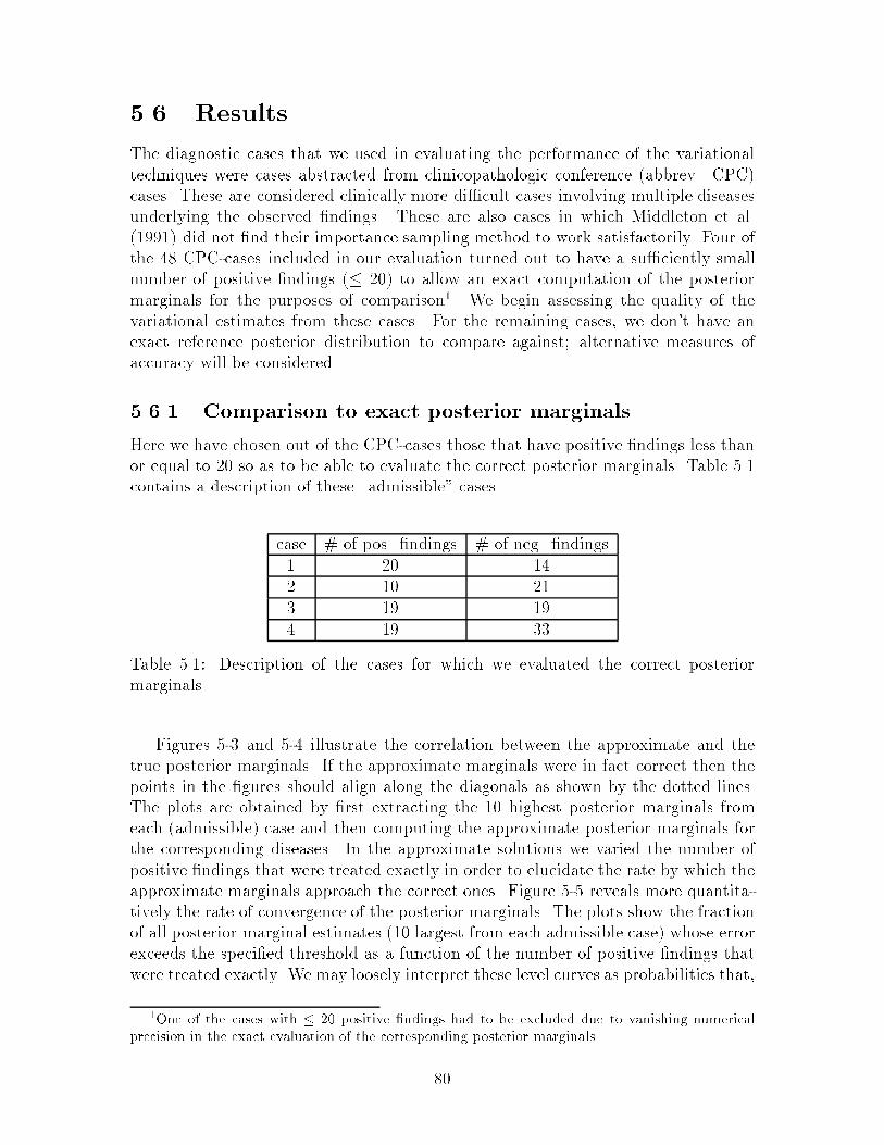
5.6 ResultsThe diagnostic cases that we used in evaluating the performance of the variationaltechniques were cases abstracted from clinicopathologic conference (abbrev. CPC)cases. These are considered clinically more di�cult cases involving multiple diseasesunderlying the observed �ndings. These are also cases in which Middleton et al.(1991) did not �nd their importance sampling method to work satisfactorily. Four ofthe 48 CPC-cases included in our evaluation turned out to have a su�ciently smallnumber of positive �ndings (� 20) to allow an exact computation of the posteriormarginals for the purposes of comparison1. We begin assessing the quality of thevariational estimates from these cases. For the remaining cases, we don't have anexact reference posterior distribution to compare against; alternative measures ofaccuracy will be considered.5.6.1 Comparison to exact posterior marginalsHere we have chosen out of the CPC-cases those that have positive �ndings less thanor equal to 20 so as to be able to evaluate the correct posterior marginals. Table 5.1contains a description of these \admissible" cases.case # of pos. �ndings # of neg. �ndings1 20 142 10 213 19 194 19 33Table 5.1: Description of the cases for which we evaluated the correct posteriormarginals.Figures 5-3 and 5-4 illustrate the correlation between the approximate and thetrue posterior marginals. If the approximate marginals were in fact correct then thepoints in the �gures should align along the diagonals as shown by the dotted lines.The plots are obtained by �rst extracting the 10 highest posterior marginals fromeach (admissible) case and then computing the approximate posterior marginals forthe corresponding diseases. In the approximate solutions we varied the number ofpositive �ndings that were treated exactly in order to elucidate the rate by which theapproximate marginals approach the correct ones. Figure 5-5 reveals more quantita-tively the rate of convergence of the posterior marginals. The plots show the fractionof all posterior marginal estimates (10 largest from each admissible case) whose errorexceeds the speci�ed threshold as a function of the number of positive �ndings thatwere treated exactly. We may loosely interpret these level curves as probabilities that,1One of the cases with � 20 positive �ndings had to be excluded due to vanishing numericalprecision in the exact evaluation of the corresponding posterior marginals.80

in a hypothetical case, the error in a posterior marginal estimate would exceed thespeci�ed limit. Figure 5-5a is in terms of the relative error in the posterior marginals;�gure 5-5b on the other hand uses the absolute error.a) 0 0.2 0.4 0.6 0.8 1

0

0.2

0.4

0.6

0.8

1

correct posterior marginals

varia

tiona

l est

imat

es b) 0 0.2 0.4 0.6 0.8 10

0.2

0.4

0.6

0.8

1

correct posterior marginals

varia

tiona

l est

imat

es

Figure 5-3: Correlation between the variational posterior estimates and the correctmarginals. In a) 4 and in b) 8 positive �ndings were treated exactly.a) 0 0.2 0.4 0.6 0.8 1

0

0.2

0.4

0.6

0.8

1

correct posterior marginals

varia

tiona

l est

imat

es b) 0 0.2 0.4 0.6 0.8 10

0.2

0.4

0.6

0.8

1

correct posterior marginals

varia

tiona

l est

imat

es

Figure 5-4: Correlation between the variational posterior estimates and the correctmarginals. In a) 12 and in b) 16 positive �ndings were treated exactly.5.6.2 Comparison to Gibbs' sampling estimatesIn this section we will compare the accuracy of the variational posterior estimates tothose obtained through stochastic procedures. Our goal here is merely to demonstratethat the variational methods are competetive with sampling techniques. For this rea-son, we chose to use a straightforward Gibbs' sampling technique in our comparisons.We emphasize, however, that many (often superior) sampling methods are available(see Shwe & Cooper 1991, Neal 1993) and our results should be viewed in this light.In our Gibbs' sampling method the posterior disease marginals were obtained fromP̂ (di) = 1T Xt P ( di j f; dt n dti ) (5.24)81

a) 5 10 15 200

0.2

0.4

0.6

0.8

1

# of exactly treated findings

err

or

fre

qu

en

cy

dp/p > 0.125

dp/p > 0.25dp/p > 0.5 b) 5 10 15 20

0

0.2

0.4

0.6

0.8

1

# of exactly treated findings

err

or

fre

qu

en

cy

dp > 0.05

dp > 0.1

dp > 0.2Figure 5-5: The fraction of posterior marginal estimates exceeding the speci�ed errorlimits as a function of the number of positive �ndings that were treated exactly. Theerror measures used were a) the relative error, and b) the absolute error.where each new disease con�guration dt was computed from the previous one dt�1through sequentially resampling the disease states with replacement. The order forthe updates was chosen randomly at each stage. For good performance only every5th such dt sample was included in the above sum. The initial con�guration d0 wasdrawn from the prior distribution over the diseases2. While discarding (a lot of)early samples is generally pro�table, it seemed to only deteriorate the results in ourcase. The accuracy gained through the use of later samples was o�set by the loss incomputation time spent for discarding the early samples (cf. the time/accuracy plotof �gure 5-6 below). Consequently no early samples were excluded.To be able to reliably assess the accuracy of the posterior estimates we usedthe four tractable cases described in the previous section. Figure 5-6 shows themean correlations (across these admissable cases) between the approximate estimatesand the correct posterior marginals as a function of the execution time needed forcomputing the estimates. The correlation measures for the stochastic method wereaveraged across 20 independent runs for each admissable case, and across these casesfor the �nal measure. The error bars in the �gure were obtained by averaging thestandard deviations computed for each admissable case from the 20 di�erent runs;the error bars therefore re ect how much the correlations would typically vary overseveral runs on the same case, i.e., they capture the repeatability of the stochasticestimates. Note that the variational estimates are deterministic and vary only acrosscases. We conclude from the �gure that more sophisticated sampling techniques areneeded to achieve a level of performance comparable to variational methods.5.6.3 Posterior accuracy across casesIn the absence of the exact posterior marginals for reference, we have to �nd a way toassess the accuracy of the estimated posterior marginals. We perform this assessmentthrough a measure of variability of these marginals. Recall �rst that in the varia-2The most likely initial con�guration was therefore the one with all the diseases absent.82

100

101

102

1030.8

0.85

0.9

0.95

1

execution time in secondsco

rrel

atio

nFigure 5-6: The mean correlation between the approximate and exact posteriormarginals as a function of the execution time (seconds). Solid line: variational esti-mates; dashed line: Gibbs' sampling. The dotted line indicates the average time forthe exact calculation of the posterior marginals in the admissable cases.tional approximation some of the conditional probabilities for the positive �ndingsare treated exactly while the remaining conditionals are replaced with their variationalcounterparts. The posterior marginals will naturally depend on which conditionalsreceived exact treatment and which were approximated. Conversely, a lack of suchdependence implies that we have the correct posterior marginals. We can thereforeuse this dependence as a way to assess the validity of the current posterior estimates.Let P̂i(di = 1) be the ith largest posterior marginal probability based on the varia-tional method, and let P̂+ki (di = 1) be a re�ned estimate of the same marginal, wherethe re�nement comes from treating the kth positive �nding exactly. As a measureof accuracy of the posterior estimates we use the variability of P̂+ki (di = 1) aroundP̂i(di = 1), where k varies in the set of positive �ndings whose conditional probabili-ties have been transformed in obtaining P̂i(di = 1). Several de�nitions can be givenfor this variability and we consider two of them below.Mean squared variabilityFor each disease we de�ne the variability of its posterior probability estimates accord-ing to �̂i2 = 1K Xk �P̂i(di = 1) � P̂+ki (di = 1)�2 (5.25)which is the mean squared di�erence between P̂i(di = 1) and its possible re�nementsP̂+ki (di = 1). The sum goes over the positive �ndings for which we have introduceda variational transformation in computing P̂i(di = 1). As an overall measure ofvariability for any particular diagnostic case, we use�̂ = maxi�10 �̂i (5.26)83

The decision to include only 10 largest posterior marginals is inconsequential butconvenient. We note that the �̂ measure is scale dependent, i.e., it assigns a highervariability to the same relative di�erence when the probabilities involved are larger.The measure therefore puts more emphasis on the posterior marginals that are likelyto be diagnostically most relevant.Before adopting the variability measure �̂ for further analysis we will �rst providesome empirical justi�cation for it. To this e�ect, we can use the admissible CPC casesconsidered in section 5.6.1 for which the exact posterior disease marginals can becomputed. We would expect the variability measure to re ect the true mean squarederror between the variational posterior estimates and the correct posterior marginals.As shown in �gure 5-7, the correlation between these measures is indeed quite good.Naturally, only the four reference cases included in the �gure are not su�cient toestablish the credibility of the variability measure but they are indicative. The a)and b) parts of the �gure, respectively, correspond to treating 8 and 12 �ndingsexactly.a) 0 0.05 0.1 0.15 0.2

0

0.05

0.1

0.15

0.2

mean squared error

varia

bili

ty m

ea

sure b) 0 0.05 0.1 0.15 0.2

0

0.05

0.1

0.15

0.2

mean squared error

varia

bili

ty m

ea

sure

Figure 5-7: The correlation between �̂ and �, where �̂ is the variability measure and� is the true mean squared error between the variational estimates and the correctmarginals. 10 most likely posterior marginals were included from each admissiblecase. The number of exactly treated �ndings was 8 in �gure a) and 12 in b).Figure 5-8 illustrates how the accuracy or the variability �̂ of the posterior esti-mates depends on the number of positive and negative �ndings across the CPC-cases.Eight conditional probabilities were treated exactly in each of the CPC-cases. Figure5-9 is analogous except that the number of exactly treated �ndings was 12. As ex-pected, the variational approximation is less accurate for larger numbers of positive�ndings (see the regression lines in the �gures). Since the number of exactly treated�ndings (or conditionals) was �xed, the more positive �ndings a case has, the morevariational transformations need to be introduced. This obviously deteriorates theposterior accuracy and this is seen in the �gures. The �gures also seem to indicatethat the variational approximations become better as the number of negative �ndingsincreases. This e�ect, however, has to do with the scale dependent measure of accu-racy. To see why, note �rst that the negative �ndings reduce the prior probabilities forthe diseases, although somewhat selectively. Smaller prior probabilities nevertheless84

decrease the posteriors marginals. The scale dependent �̂ therefore decreases with-out any real improvement of the variational accuracy. The �gure 5-9 is included incomparison to indicate that indeed the error measure is consistently lower when more�ndings have been treated exactly. We note �nally that the squared error measurefor the posterior marginals is generally quite small; large deviations from the truemarginals are therefore rare.a) 10 20 30 40 50 60 70

0

0.05

0.1

0.15

0.2

0.25

# of positive findings

varia

bilit

y m

easu

re b) 0 10 20 30 40 500

0.05

0.1

0.15

0.2

0.25

# of negative findings

varia

bilit

y m

easu

reFigure 5-8: a) The variability �̂ of the posterior marginals as a function of the numberpositive �ndings in the CPC-cases. b) The same variability measure �̂ but now as afunction of the number of negative �ndings. 8 positive �ndings were treated exactlyfor this �gure.

a) 10 20 30 40 50 60 700

0.05

0.1

0.15

0.2

0.25

# of positive findings

varia

bilit

y m

easu

re b) 0 10 20 30 40 500

0.05

0.1

0.15

0.2

0.25

# of negative findings

varia

bilit

y m

easu

re

Figure 5-9: a) The variability �̂ of the posterior marginals as a function of the numberpositive �ndings in the CPC-cases. b) The same variability measure �̂ but now as afunction of the number of negative �ndings. Now 12 positive �ndings were handledexactly.Min/Max variability across casesWhile the squared error captures the mean variability in the posterior estimates, it isimportant to �nd out the limits of how much the true posterior marginals could devi-ate from our estimates. We use the bounds mink P̂+ki (di = 1) and maxk P̂+ki (di = 1)85

as indicators of this deviation. While these variability bounds do not provide rigorousbounds on the posterior disease marginals they nevertheless come close to doing so inpractice. To substantiate this claim, we used the four CPC cases considered in section5.6.1. Figure 5-10 illustrates the accuracy of these bounds for 10 most likely posteriormarginals from each of the four cases. Although few of the posterior marginals dofall outside of these bounds, the discrepancies are quite minor and even in these casesthe bounds provide an indication of the direction of the error between the correct andthe estimated posterior marginals. Moreover, when the bounds are tight, the trueposterior marginals appear within or very close to the bounds.While the bounds provide a measure of accuracy for individual posterior estimates,we employ a correlation measure to indicate the overall accuracy. In other words, weuse the correlation between the variational posterior estimates and the min/maxbounds of the re�ned marginals as the overall measure. A high degree of correlationindicates that the posterior probabilities are very accurate; otherwise, at least one ofthe positive �ndings should in uence the re�ned posterior marginals and consequentlythe bounds thereby deteriorating the correlation. Recall that each positive �nding istreated exactly in one of the re�ned marginals. We note that this correlation measureis deterministic.a) 0 0.2 0.4 0.6 0.8 1

0

0.2

0.4

0.6

0.8

1

correct posterior marginals

min

/max

bou

nds b) 0 0.2 0.4 0.6 0.8 1

0

0.2

0.4

0.6

0.8

1

correct posterior marginals

min

/max

bou

nds

Figure 5-10: The correlation between the min/max bounds and the true posteriormarginals. 10 most likely posterior marginals were included from each admissiblecase. In a) 8 �ndings were treated exactly and in b) 12.Figure 5-11a illustrates the correlation between the variational posterior marginalsand the min/max bounds of the re�ned marginals for the CPC cases. The cor-relation coe�cients when 8 �ndings were treated exactly for each diagnostic casewere 0:953=0:879 between the approximate marginals and those of the min/maxbounds, respectively. When 12 �ndings were included exactly these coe�cients roseto 0:965=0:948 (see �gure 5-11b). The dependence of the correlation coe�cients onthe number of exactly treated positive �ndings is illustrated in �gure 5-12a. Thehigh monotonic increase in the correlation is mainly due to the proper ordering of the�ndings to be treated exactly (see section 5.4.2). In comparison, �gure 5-12b showsthe development of the correlations for a random ordering.86

a) 0 0.2 0.4 0.6 0.8 10

0.2

0.4

0.6

0.8

1

variational posterior estimates

min

/ma

x re

fine

d e

stim

ate

s

b) 0 0.2 0.4 0.6 0.8 10

0.2

0.4

0.6

0.8

1

variational posterior estimates

min

/ma

x re

fine

d e

stim

ate

s

Figure 5-11: a) Correlation between the estimated posterior marginals and themin/max re�ned marginals. There were 8 positive �ndings considered exactly. b)as before but now the number of �ndings treated exactly was 12.a) 2 4 6 8 10 12

0

0.2

0.4

0.6

0.8

1

# of exactly treated findings

corr

ela

tion b) 2 4 6 8 10 12

0

0.2

0.4

0.6

0.8

1

# of exactly treated findings

corr

ela

tionFigure 5-12: Mean correlation between the approximate posterior marginals and themin/max bounds as a function of the number of positive �ndings that were treatedexactly. Solid line: correlation with the max- bound; dashed line: correlation withthe min- bound. Figure a) is for the case where a proper ordering was used to selectthe �ndings to be treated exactly and in b) a random ordering was used.5.6.4 Execution timesWe report here additional results on the feasibility of the variational techniques interms of computation time. The results were obtained on a Sun Sparc 10 workstation.The execution times for obtaining the variational posterior estimates are over-whelmingly dominated by the number of exactly treated positive �ndings, i.e., theamount of exact probabilistic calculations. The time needed for the variational op-timization using the shortcut discussed at the end of Appendix 5.A is insigni�cant.The maximum time across the CPC-cases was less than 2 seconds whenever at most12 positive �ndings were treated exactly.More relevant in a practical setting is the combined time of obtaining the posteriorestimates and carrying out the verifying analyses as described in the previous sections.Figure 5-13 plots the mean and the maximum execution times across the CPC-cases87

for such analyses as a function of the number of positive �ndings that were treatedexactly. The mean time when 12 �ndings were treated exactly was about 1 minuteand the maximum about 2 minutes.0 2 4 6 8 10 12

0

20

40

60

80

100

120

140

# of exactly treated findings

exe

cutio

n t

ime

Figure 5-13: Mean (solid line) and maximum (dashed line) execution times in secondsfor the analyses of section 5.6.2 across the CPC-cases as a function of the number ofexactly treated positive �ndings.5.7 DiscussionThe bene�ts of probabilistic models and reasoning comes from the rigorous semanticsthat underlies them. Increasingly complex probabilistic models such as the QMR-DTbelief network, however, necessitate the use of approximate techniques in evaluat-ing the probabilities or quantities implied by the probabilistic framework. We havedemonstrated in this chapter that variational methods can be employed as viable al-ternatives to sampling techniques that are more traditionally used towards such goals.We maintain, however, that our results are preliminary and resort to one out of manypossible techniques. For example, the feasibility of obtaining rigorous bounds on theposterior disease marginals through variational methods was only partially exploitedin the current work. Such bounds become perhaps even more important in fully de-cision theoretic systems, towards which QMR-DT is being developed. This chaptertherefore characterizes merely the potential of variational methods for probabilisticreasoning in important application domains such as in medicine.AcknowledgmentsWe would like to thank the University of Pittsburgh and Randy Miller for the use ofthe QMR database. 88

ReferencesB. D'Ambrosio (1994). Symbolic probabilistic inference in large BN20 networks. InProceedings of the Tenth Conference on Uncertainty in Arti�cial Intelligence. MorganKaufmann.J. Bucklew (1990). Large deviation techniques in decision, simulation, and estimation.John Wiley & Sons.G. Cooper (1990). The computational complexity of probabilistic inference usingBayesian belief networks. Arti�cial Intelligence 42:393-405.F. Jensen (1996). Introduction to Bayesian networks. Springer.B. Middleton, M. Shwe, D. Heckerman, M. Henrion, E. Horvitz. H. Lehmann, G.Cooper (1991). Probabilistic diagnosis using a reformulation of the INTERNIST-1/QMR knowledge base: Part-II. Stanford University technical report.R. Neal (1993). Probabilistic inference using Markov chain Monte Carlo methods.Technical report CRG-TR-93-1, University of Toronto.M. Shwe and G. Cooper (1991). An empirical analysis of Likelihood { weightingsimulation on a large, multiply connected medical belief network. Computers andBiomedical Research 24:453-475.M. Shwe, B. Middleton, D. Heckerman, M. Henrion, E. Horvitz. H. Lehmann, G.Cooper (1991). Probabilistic diagnosis using a reformulation of the INTERNIST-1/QMR knowledge base: Part-I. Methods of Information in Medicine 30: 241-255.5.A Optimization of the variational parametersThe metric for optimizing the variational parameters comes from the bounding prop-erties of the individual variational transformations introduced for the conditionalprobabilities. Each transformation is an upper bound on the corresponding condi-tional and therefore also the resulting joint distribution is an upper bound on thetrue joint; similarly all marginals such as the likelihood of the positive �ndings thatare computed from the new joint will be upper bounds on the true marginals. ThusP (f+) =Xd P (f+jd)P (d) � Xd P (f+jd; �)P (d) = P (f+j�) (5.27)and we may take the accuracy of P (f+j�), the variational likelihood of observations,as a metric. To simplify the ensuing notation we assume that the �rst m of thepositive �ndings have been transformed (and therefore need to be optimized) while theremaining conditional probabilities will be treated exactly. In this notation P (f+j�)89

is given by P (f+j�) = Xd 24Yi�mP (f+i jd; �i)35 "Yi>mP (f+i jd)#Yj P (dj) (5.28)/ E 8<:Yi�mP (f+i jd; �i)9=; (5.29)where the expectation is over the posterior distribution for the diseases given thosepositive �ndings that we plan to treat exactly. Note that the proportionality con-stant does not depend on the variational parameters; it is the likelihood of the exactlytreated positive �ndings. We now insert the explicit forms of the transformed condi-tional probabilities (see Eq. (5.12)) into Eq. (5.29) and �ndP (f+j�) / E8<:Yi�m e �i(�i0+Pj �ijdj)�f�(�i)9=; (5.30)= ePi�m(�i�i0�f�(�i))E �ePj; i�m �i�ijdj� (5.31)where we have simply the products over i into sums in the exponent and pulled outthe terms that are independent of the expectation. On a log-scale, the proportionalitybecomes an equivalence up to a constant:logP (f+j�) = C + Xi�m (�i�i0 � f�(�i)) + logE �ePj;i�m �i�ijdj� (5.32)Several observations are in order. Recall that f�(�i) is the conjugate of the concavefunction f (the exponent), and is therefore also concave; for this reason �f�(�i) isconvex. We claim that the remaining termlogE �ePj;i�m �i�ijdj� (5.33)is also a convex function of the variational parameters. The justi�cation for this canbe found either in Appendix 1.A of chapter 1 or Appendix 2.A of chapter 2 (it is alsowell-known in the physics literature). Since any sum of convex functions stays convex,we conclude that log P (f+j�) is a convex function of the variational parameters. Im-portantly, this means that there are no local minima and the optimal or minimizing �can be always found. We may safely employ the standard Newton-Raphson procedureto solve r logP (f+j�) = 0. For simplicity, we may equivalently iteratively optimizethe individual variational parameters, i.e., for each �k solve @=@�k logP (f+j�) = 0.In this case, the relevant derivatives consists of (algebra omitted):@@�k log P (f+j�) = �k0 + log �k1 + �k + E 8<:Xj �kjdj9=; (5.34)90

@2@2�k log P (f+j�) = 1�k � 11 + �k + V ar8<:Xj �kjdj9=; (5.35)Here the expectation and the variance are with respect to the same posterior distri-bution as before, and both derivatives can be computed in time linear in the numberof associated diseases for the �nding. We note that the benign scaling of the variancecalculations comes from exploiting the special properties of the noisy-OR dependenceand the marginal independence of the diseases. The convexity of the log-likelihood(with respect to �k) is evident from the expression for the second derivative (i.e., itis always positive).To further simplify the optimization procedure, we can simply set the variationalparameters to values optimized in the context where all the positive �ndings havebeen transformed. While such setting is naturally suboptimal for cases where thereare exactly treated positive �ndings, the incurred loss in accuracy is typically quitesmall. The gain in computation time can, however, be considerable especially whena large number of positive �ndings are treated exactly; the expectations above canbe exponentially costly in the number of such positive �ndings (see Eq. (5.5)). Thesimulation results reported in this chapter have been obtained using this shortcutunless otherwise stated.5.B Accuracy and the leak probabilityHere we prove that any increase in the leak probability improves the accuracy ofthe variational transformation. Such increase of the leak probability can happen,for example, as a result of conditioning the likelihood of the observed �ndings onthe presence of some of the diseases (see the calculation of the posterior marginalprobabilities in the text). Now, for the accuracy to improve as a function of the leakprobability (or the bias term in the exponentiated notation) means that the followinglog-likelihood ratio has to be a decreasing function of the bias �:ratio(�) = log min� E ne�(Pj �ijdj+�)�F (�)oE n1� e�Pj �ijdj��o = log min� E ne�(x+�)�F (�)oE f1� e�x��g (5.36)where the expectations are with respect to the posterior distribution over the diseasesbased on all other observed �ndings except for the positive �nding i. We have adoptedthe simpli�ed notation x = Pj �ijdj since the linear form plays no role in the proof.We note that it su�ces to show that the derivative of ratio(�) is negative at � = 0.The negativity of this derivative for other values of � follows simply by rede�ning x(i.e, x x+ �), and the fact that the proof does not depend on the distribution overx. To �x ideas, we start from the observation that since the variational transforma-91

tion is optimized with respect to � at � = 0 we must have@@�E ne�x�F (�)o = e�F (�) "E nxe�xo� @F (�)@� E ne�xo# = 0 (5.37)The fact that @F (�)=@� = � log(�=(� + 1)) allows us to obtain an implicit solutionfor � from the above equation giving� = e�~x1� e�~x ; where ~x = E nxe�xoE fe�xg (5.38)~x can be seen to be the mean of x with respect to the twisted or tilted distribution.It is well-known in the large deviation literature that ~x � Efxg (see e.g. Bucklew,1990). To use this property we �rst di�erentiate ratio(�) with respect to � and �nd:@@�ratio(�) = � � E fe�xg1 � E fe�xg (5.39)where the implicit derivatives vanish due to the optimization of �. As z=(1� z) is anincreasing function of z and since e�x is a convex function of x, i.e., E fe�xg � e�Efxg,it follows that E fe�xg1� E fe�xg � e�Efxg1� e�Efxg (5.40)Finally, combining the results from Eq. (5.38), Eq. (5.39), and Eq. (5.40) with thefact that e�x is a decreasing function gives@@�ratio(�) = e�~x1 � e�~x � E fe�xg1 � E fe�xg � e�~x1 � e�~x � e�Efxg1 � e�Efxg � 0 (5.41)This completes the proof.92

Chapter 6DiscussionGraphical models remain useful as knowledge representations to the extent that weare able to carry out inferences in these models or learn on the basis of observations.The increasing complexity of the models in important application areas, however,necessitate the use of approximate techniques to reap the bene�ts from the prob-abilistic representations. We have provided in this thesis a framework for approx-imating graphical models in a principled way through variational transformations.The preceding chapters contain the development of this approximation methodologyfor probabilistic inference, Bayesian estimation, and for diagnostic reasoning in thecontext of the QMR-DT belief network.Probabilistic inference: In chapter 2 we laid the foundation for obtaining upper andlower bounds on probabilities and subsequently in chapter 3 removed the topologi-cal constraints from such bounds by introducing the relevant transformations recur-sively. The recursive methods proposed in chapter 3 are currently constrained by theavailable transformations. The framework nevertheless provides the basis for furtherdevelopment of these transformations.Relevant to this framework is the role that the variational bounds play in deter-mining the approximation accuracy. If the interval estimate speci�ed by the comple-mentary bounds is tight then necessarily the approximation is reliable. The converse,however, is not true in general. By this we mean that the marginal estimates1 ob-tained through one of the bounds need not be inaccurate even if the interval estimateis too wide to be useful. The aspect that is lost due to wide intervals is the guaranteeof reliability, not the accuracy directly. In the absence of useful intervals, the boundswill nevertheless retain their error metric (boundedness), and they can be re�ned ac-cording to this metric. It is only by mixing upper bounds with lower bounds that welose the metric as well and, consequently, all the bene�ts accompanying variationalmethods over other approximation techniques.Another issue to consider is the nature of the variational transformations we haveused. Is the convexity framework too restrictive? Many variational transformationsproducing strict bounds can be viewed as manifestations of underlying convexity1Note that the marginal estimate based on either upper or lower bound are found simply bynormalizing the expression for the corresponding bound.93

representations through reparametrization (cf. the mean �eld derivation in Appendix4.39). More to the point is the question whether it is convenient to establish therelation { assuming it exists { to convex duality. This, of course, is not always thecase.We have also largely disregarded the issue of possible semantic losses resultingfrom the use of variational approximation techniques: which independence propertieswill be lost and which are imposed by the variational framework? While impor-tant, the question as posed is somewhat ambiguous since the answer depends on theoptimization schedule adopted for the variational parameters. For example, if theoptimization is performed conditionally on each con�guration of the variables in theprobability model, we retain the exact model. The way to investigate this issue isto concentrate on actual bounds on marginal probabilities, where the variational pa-rameters are optimized conditionally on each marginal con�guration. Normalizingsuch a bound yields a marginal distribution whose independence properties can becharacterized.Bayesian estimation: The Bayesian formalism for parameter estimation can be par-ticularly useful in the extreme cases of scarce data or when the amount of data isoverwhelming, both of which are likely to arise in modern environments. In the for-mer case, the bene�t comes from the ease of embedding prior knowledge into theparameter values, while in the latter the advantage relies on the sequentiality of theestimation procedure. Computationally, however, the Bayesian framework is quitecostly and often infeasible. We demonstrated in chapter 4 that variational methodscan provide e�cient and principled approximations to re-establish the utility of theBayesian formalism, particularly in the presence of missing values.Applications: The preliminary application of the variational methods to the QMR-DTbelief network illustrates the potential in these techniques for large scale applications.We did not fully utilize the power of the methodology, however, and the calculationof rigorous bounds on the posterior marginals in the QMR setting remains an issuefor future work.We have deferred the discussion about sampling methods in comparison to thevariational ones here as such considerations seem most appropriate in the context ofapplications. While sampling techniques enjoy wider (or at least more immediate)applicability, they also appear to be less able to bene�t from the structure of a par-ticular model; nor do they attain bounds or analyzable expressions for the quantitiesof interest. It is also straightforward and pro�table to combine variational methodswith exact calculations, whereas with sampling techniques it is less apparent how thiscan be done e�ciently. Extensive comparisons between these methods will be neededto resolve the domain characteristics in which one is preferable to the other. Wenote �nally that the two frameworks need not be mutually exclusive: the variationalestimates could be used, for example, as importance sampling distributions, whichhas been suggested by many people. 94