computing extremely accurate quantiles using t-digests · computing extremely accurate quantiles...

COMPUTING EXTREMELY ACCURATE QUANTILES USING

t-DIGESTS

TED DUNNING AND OTMAR ERTL

Abstract. Two variants of an on-line algorithm for computing approximations of rank-

based statistics are presented that allow controllable accuracy, particularly near the tails

of the distribution. Moreover, this new algorithm can be used to compute hybrid statistics

such as trimmed means in addition to computing arbitrary quantiles. An unusual property

of the method is that it allows a quantile q to be computed with an accuracy relative to

max(q, 1 − q) rather than with an absolute accuracy as with most methods. This new

algorithm is robust with respect to highly skewed distributions or highly ordered datasets

and allows separately computed summaries to be combined with no loss in accuracy.

An open-source Java implementation of this algorithm is available from the author.

Implementations in Go and Python are also available.

1. Introduction

Given a set of numbers, it is often desirable to compute rank-based statistics such as the

median, 95-th percentile or trimmed means in an on-line fashion. In many cases, there is

an additional requirement that only a small data structure needs to be kept in memory as

data is processed in a streaming fashion. Traditionally, such statistics have been computed

by sorting the data and then either finding the quantile of interest by interpolation or by

re-processing all samples within particular quantile ranges. This sorting approach can be

infeasible for very large datasets or when quantiles of many subsets must be calculated. This

infeasibility has led to interest in on-line approximate algorithms. Previous algorithms can

compute approximate values of quantiles using constant or only weakly increasing memory

footprint, but these previous algorithms cannot provide constant relative accuracy. The

new algorithm described here, the t-digest, provides constant memory bounds and constant

relative accuracy while operating in a strictly on-line fashion.

1.1. Previous work. One early algorithm for computing on-line quantiles is described by

Chen, Lambert and Pinheiro in [CLP00]. In that work specific quantiles were computed1

2 TED DUNNING AND OTMAR ERTL

by incrementing or decrementing an estimate by a value proportional to the simultane-

ously estimated probability density at the desired quantile. This method is plagued by

a circularity in that estimating density is only possible by estimating yet more quantiles.

Moreover, this work did not allow the computation of hybrid quantities such as trimmed

means.

Munro and Paterson[MP80] provided an alternative algorithm to get a precise estimate

of the median. This is done by keeping s samples from the N samples seen so far where

s << N by the time the entire data set has been seen. If the data are presented in random

order and if s = θ(N1/2 logN), then Munro and Paterson’s algorithm has a high probability

of being able to retain a set of samples that contains the median. This algorithm can be

adapted to find a number of pre-specified quantiles at the same time at proportional cost

in memory. The memory consumption of Munro-Paterson algorithm is, however, excessive

if precise results are desired. Approximate results can be had with less memory, however.

A more subtle problem is that the implementation of Munro and Paterson’s algorithm

in Sawzall[PDGQ05] and the Datafu library[Lin] uses a number of buckets computed from

the GCD of the desired quantiles. This means that if you want to compute the 99-th, 99.9-

th and 99.99-th percentiles, a thousand buckets are required, each of which requires the

retention of many samples. We will refer to this implementation of Munro and Paterson’s

algorithm as MP01 in results presented here.

One of the most important results of the work by Munro and Paterson was a proof that

computing any particular quantile exactly in p passes through the data requires Ω(N1/p)

memory. For the on-line case, p = 1, which implies that on-line algorithms cannot guaran-

tee to produce the precise value of any particular quantile. This result together with the

importance of the on-line case drove subsequent work to focus on algorithms to produce

approximate values of quantiles.

Greenwald and Khanna[GK01] provided just such an approximation algorithm that is

able to provide estimates of quantiles with controllable accuracy. This algorithm (which

we shall refer to as GK01 subsequently in this paper) requires less memory than Munro

and Paterson’s algorithm and provides approximate values for pre-specified quantiles.

An alternative approach is described by Shrivastava and others in [SBAS04]. In this

work, incoming values are assumed to be integers of fixed size. Such integers can trivially

be arranged in a perfectly balanced binary tree where the leaves correspond to the integers

and the interior nodes correspond to bit-wise prefixes. This tree forms the basis of the data

COMPUTING EXTREMELY ACCURATE QUANTILES USING t-DIGESTS 3

structure known as a Q-digest. The idea behind a Q-digest is that in the uncompressed case,

counts for various values are assigned to leaves of the tree. To compress this tree, sub-trees

are collapsed and counts from the leaves are aggregated into a single node representing the

sub-tree such that the maximum count for any collapsed sub-tree is less than a threshold

that is a small fraction of the total number of integers seen so far. Any quantile can be

computed by traversing the tree in left prefix order, adding up counts until the desired

fraction of the total is reached. At that point, the count for the last sub-tree traversed can

be used to interpolate to the desired quantile within a small and controllable error. The

error is bounded because the count for each collapsed sub-tree is bounded.

The salient virtues of the Q-digest are

• the space required is bounded proportional to a compression factor k

• the maximum error of any quantile estimate is proportional to 1/k and

• the desired quantiles do not have to be specified in advance.

On the other hand, two problems with the Q-digest are that it depends on the set of

possible values being known in advance and produces quantile estimates with constant

error in q. In practice, this limits application of the Q-digest to samples which can be

identified with the integers. Adapting the Q-digest to use a balanced tree over arbitrary

elements of an ordered set is difficult. This difficulty arises because rebalancing the tree

involves sub-tree rotations and these rotations may require reapportionment of previously

collapsed counts in complex ways. This reapportionment could have substantial effects on

the accuracy of the algorithm and in any case make the implementation much more complex

because the concerns of counting cannot be separated from the concerns of maintaining a

balanced tree.

1.2. New contributions. The work described here introduces a new data structure known

as the t-digest. The t-digest differs from previous structures designed for computing ap-

proximate quantiles in several important respects. First, although data is binned and

summarized in the t-digest, the range of data included in different bins may overlap. Sec-

ond, the bins are summarized by a centroid value and an accumulated weight representing

the number of samples contributing to a bin. Third, the samples are accumulated in such a

way that only a few samples contribute to bins corresponding to extreme quantiles so that

relative error is bounded instead of maintaining constant absolute error as with previous

methods.


With the t-digest, accuracy for estimating the q quantile is constant relative to q(1− q).This is in contrast to earlier algorithms which had errors independent of q. The relative

error bound of the t-digest is convenient when computing quantiles for q near 0 or 1 as is

commonly required. As with the Q-digest algorithm, the accuracy/size trade-off for the

t-digest can be controlled by setting a single compression parameter δ with the amount of

memory required proportional only to Θ(δ).

2. The t-digest

A t-digest represents the empirical distribution of a set of numbers by retaining centroids

of sub-sets of numbers. Algorithmically, there are two important ways to form a t-digest

from a set of numbers. One version keeps a buffer of incoming samples. Periodically, this

buffer is sorted and merged with the centroids computed from previous samples. This

merging form of the t-digest algorithm has the virtue of allowing all memory structures

to be allocated statically. On an amortized basis, this buffer-and-merge algorithm can be

very fast especially if the input buffer is large. The other major t-digest algorithm is more

akin to a clustering algorithm in which new samples are selectively added to the nearest

centroid. Both algorithms are described here and implementations for both are widely

available.

2.1. The basic concept. Suppose first, for argument’s sake, that all of the samples X =

x1 . . . xn are presented in ascending order. Since the samples are ordered, we can use

interpolation on the indexes of each sample to determine the value of the empirical quantile

for any new value.

A t-digest is formed from the sequence of points by grouping all of the samples into sub-

sequences of samples, X = s1|s2| . . . |sm where si = xleft(i) . . . xright(i). The beginning

and end of each sub-sequence is chosen so that the sub-sequence is small enough to get

accurate quantile estimates by interpolation, but large enough so that we don’t wind up

with too many sub-sequences. Importantly, we force sub-sequences near the ends to be

small while allowing sub-sequences in middle to be larger in order to get fairly constant

relative accuracy.

To limit the sub-sequence size in this way, we define a mapping from quantile q to a

notional index k with compression parameter δ. This mapping is known as the scaling


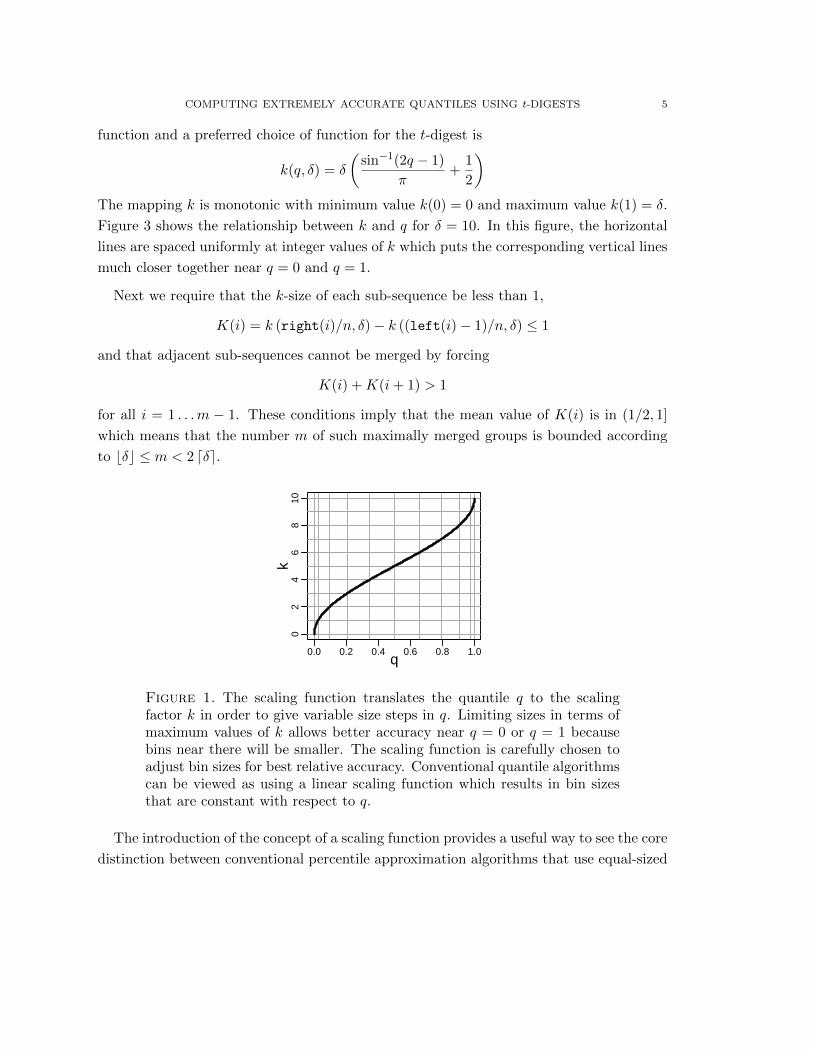
function and a preferred choice of function for the t-digest is

k(q, δ) = δ

(sin−1(2q − 1)

π+

1

2

)The mapping k is monotonic with minimum value k(0) = 0 and maximum value k(1) = δ.

Figure 3 shows the relationship between k and q for δ = 10. In this figure, the horizontal

lines are spaced uniformly at integer values of k which puts the corresponding vertical lines

much closer together near q = 0 and q = 1.

Next we require that the k-size of each sub-sequence be less than 1,

K(i) = k (right(i)/n, δ)− k ((left(i)− 1)/n, δ) ≤ 1

and that adjacent sub-sequences cannot be merged by forcing

K(i) +K(i+ 1) > 1

for all i = 1 . . .m − 1. These conditions imply that the mean value of K(i) is in (1/2, 1]

which means that the number m of such maximally merged groups is bounded according

to bδc ≤ m < 2 dδe.

0.0 0.2 0.4 0.6 0.8 1.0q

02

46

810

k

Figure 1. The scaling function translates the quantile q to the scalingfactor k in order to give variable size steps in q. Limiting sizes in terms ofmaximum values of k allows better accuracy near q = 0 or q = 1 becausebins near there will be smaller. The scaling function is carefully chosen toadjust bin sizes for best relative accuracy. Conventional quantile algorithmscan be viewed as using a linear scaling function which results in bin sizesthat are constant with respect to q.

The introduction of the concept of a scaling function provides a useful way to see the core

distinction between conventional percentile approximation algorithms that use equal-sized


bins and the t-digest with its non-equal bin sizes. The only really necessary characteristics

of a scaling function is that be monotonic and satisfy the constraints that k(0) = 0 and

k(1) = δ. A linear function k(q) = δq clearly meets these requirements and thus would

be an acceptable scaling function. Using a linear scaling function results in uniform bin

sizes and constant absolute error just as in previously reported quantile approximation

algorithms. The t-digest, in contrast, has a non-linear scaling function which was chosen

to give non-equal bin sizes and constant relative accuracy.

Once we have formed a t-digest by binning the original sequence into sub-sequences that

satisfy the size limit, we can estimate quantiles using interpolation between the end-points

of each bin. This is similar to what is done in other quantile estimation algorithms such

as Greenwald-Khanna and will give errors that scale roughly quadratically in the number

of samples in each sub-sequence. The t-digest, having smaller number of samples in bins

near q = 0 or q = 1 will obviously have better accuracy there. The only wrinkle is that

with a t-digest contains the centroids of the samples in a bin instead of the end-points.

Estimating quantiles requires that the boundaries of the bins be estimated first and then

used to interpolate as before.

In general, there are many possible partitions of X that form a valid t-digest. As long as

the result is subject to the size contraint, however, any such t-digest will perform similarly

in terms of accuracy.

Figure 4 shows an example of how error bounds are improved by the strategy of keeping

bins small near extreme values of q.

This figure shows roughly the first percentile of 10, 000 data points sampled using x ∼log u where u ∼ Uniform(0, 1). In the left panel, the data points have been divided into

100 bins, each with 100 data points, of which only the left-most bin is visible. The use of

equal sized bins means that the interpolated value of q in the left panel of the figure has

a substantial and unavoidable error. The right panel, on the other hand, shows a t-digest

with roughly the same number of bins (102 instead of 100), but with many fewer points in

bins near the q = 0. A value of δ = 100 is used here which is quite typical in practical use.

Of course, since we have to put every sample into some bin, filling some bins with fewer

than 100 samples requires that other bins must have more than 100 samples or we have

to have more bins. Importantly, having fewer samples in the bins near the ends improves

accuracy substantially, but increasing the bin sizes near q = 1/2 has a much weaker effect

on accuracy. In this particular example, the first bin has only 2 samples and thus zero error


0.00

00.

004

0.00

8

x

q100

F

x

q

28

19

35

Figure 2. The left panel shows linear interpolation of a cumulative distri-bution function near q = 0 with 100 equal sized bins applied to 10, 000 datapoints sampled from an exponential distribution. The right panel showsthe same interpolation with variable size bins as given by a t-digest withδ = 100. The numbers above the data points represent the number of pointsin each bin.

and the second bin has only 10 samples giving 100 times smaller error while the central

bins in the t-digest have about 1.6 times more samples than the uniform case, increasing

errors by about two and a half times relative to equal sized bins. The overall effect is that

quantile estimation accuracy is dramatically improved at the extremes but only modestly

impaired in the middle of the distribution.

2.2. Merging independent t-digests. In the previous section, the algorithm for forming

a t-digest took a set of unweighted points as inputs. Nothing, however, would prevent the

algorithm from being applied to a set of weighted points. As long as individual weights

are smaller than the size limit imposed by the scaling function, the result will still be a

well-formed t-digest.

If we form independent t-digests tX and tY from separate sequences X and Y , these t-

digests can clearly be used to estimate quantiles of X∪Y by separately computing quantiles

for X and Y and combining the results. More usefully, however, we can form a new t-digest

by taking the union of the centroids from tX and tX and merging the centroids whenever

they meet the size criterion. The resulting t-digest will not necessarily be the same as if

we had computed a t-digest tX∪Y from all of the original data at once even though it will

meet the same size constraint. Because it meets the same size constraint, a merged t-digest

gives accuracy comparable to what we would get from tX∪Y while still having the same

size bound.


The observation that t-digests formed by merging other digests will produce accurate

quantile estimates has substantial empirical support, even with highly structured data sets

such as ordered data or data with large numbers of repeated values, but there is, as yet,

no rigorous proof of any accuracy guarantees. The size bounds are, nevertheless, well

established.

The ability to merge t-digests makes parallel processing of large data-sets relatively

simple since independent t-digests can be formed from disjoint partitions of the input data

and then combined to get a t-digest representing the complete data-set.

A similar divide and conquer strategy can be used to allow t-digests to be used in

OLAP systems. The idea is that queries involving quantiles of subsets of data can be

approximated quickly by breaking the input data set into subsets corresponding to each

unique combination of selection factors. A single t-digest is then pre-computed for each

unique combination of selection factors. To the extent that all interesting queries can be

satisfied by disjoint unions of such primitive subsets, the corresponding t-digests can be

combined to compute the desired result.

2.3. Progressive merging algorithm. The observation that merging t-digests gives

good accuracy suggests a practical algorithm for constructing a t-digest from a large amount

of data. The basic idea is to collect data in a buffer. When the buffer fills, or when a final

result is required, sort the buffer and any existing centroids together, and pass through

the combined set of points and centroids, merging points or centroids together whenever

the size limits can be satisfied by the merged value. With an arbitrarily large buffer, this

algorithm reduces to the original approach for constructing a t-digest from sorted data

since the overall effect is simply a single merging pass through all the data. For smaller

buffer sizes, however, many merge passes are required to process a large amount of data.

This is essentially equivalent to forming independent t-digests on buffers of data and then

sequentially merging them to get the final result.

The operation of merging a buffer’s worth of samples into an existing set of centroids is

shown in Algorithm 1. Note that the check on the size bound is optimized to only require

as many evaluations of k(q) during the merge as there are output values in C ′. This is done

by computing the bounding value qlimit = k−1(k(q, δ) + 1, δ) each time a new centroid is

emitted. This allows the conditional to be triggered based on comparisons of q so that if

many points are merged, no additional calls to k are needed. If n 2 dδe, this can result in

a considerable speedup since computing sin−1 is expensive. Note also that this algorithm


allows static allocation of all data structures as four arrays of primitive values, avoiding

any dynamic allocation or structure boxing/unboxing.

Algorithm 1: Merging new data into a t-digest

Input: Sequence C = [c1 . . . cm] a t-digest containing real-valued, weighted centroidswith components sum and count arranged in ascending order by mean, databuffer X = x1, . . . xn of real-valued, weighted points, and compression factor δ

Output: New ordered set C ′ of weighted centroids forming a t-digest1 X ← sort(C ∪X);

2 S =∑

i xi.count;

3 C ′ = [ ], q0 = 0;

4 qlimit = k−1(k(q0, δ) + 1, δ);

5 σ = x1;

6 for i ∈ 2 . . . (m+ n) :7 q = q0 + (σ.count + xi.count)/S;

8 if q ≤ qlimit :9 σ ← σ + xi;

10 else:11 C ′.append(σ);

12 q0 ← q0 + σ.count/S;

13 qlimit ← k−1(k(q0, δ) + 1, δ);

14 σ ← xi;

15 C ′.append(σ);

16 return C ′

The run-time cost of the merge variant of the t-digest is a mixture of the frequent buffer

inserts and the rare periodic merges. The buffer inserts are very fast since they consist of

an array write, index increment and an overflow test. The merges consist of the buffer sort

and the merge itself. The merge involves a scan through both the buffer and the existing

centroids plus a number of calls to sin−1 roughly equal to the size of the result and thus

bounded by 2dδe. If k1 is the input buffer size, the dominant costs are the sort and the

sin−1 calls so the amortized cost per input value is roughly C1 log k1 + C2dδe/k1 where

C1 and C2 are parameters representing the sort and sin−1 costs respectively. This overall

amortized cost has a minimum where k1 ≈ δ C2/C1. The constant of proportionality should

be determined by experiment, but micro-benchmarks indicate that C2/C1 is in the range

from 5 to 20 for a single core of an Intel i7 processor. In these micro-benchmarks, increasing

the buffer size to 10dδe dramatically improves the average speed but further buffer size


increases have much less effect. It is difficult to build a high quality approximation of sin−1

without using other high cost functions such as a square root, but by limiting the range

where the approximation is used to q ∈ [ε, 1 − ε], where ε ≈ 0.01, simple approximations

are available and the amortized benefit is nearly the same.

2.4. The clustering variant. If we allow the buffer in the merging variant of the t-digest

algorithm to contain just a single element so that merges take place every time a new point

is added, the algorithm takes on a new character and becomes more like clustering than

buffering and merging.

The basic outline of the clustering algorithm for constructing a t-digest is quite simple.

An initially empty ordered list of centroids, C = [c1 . . . cm] is kept. Each centroid consists

of a mean and a count. To add a new value xn with a weight wn, the set of centroids is

found that have minimum distance to xn. This set is reduced by retaining only centroids

whose K size after adding wn would be less than 1. If more than one centroid remains, the

one with maximum weight is selected. If a centroid is found, then the new point, (xn, wn),

is added to that centroid. If no satisfactory centroid is found then (xn, wn) is used to form

a new centroid with weight wn and the next point is considered. The K size of cluster

ci ∈ C is defined as before as

K(ci) = k(∑

j≤iwj , δ

)− k(∑

j<i

wjδ)

This clustering variant is shown more formally as Algorithm 2.

In this algorithm, a centroid object contains a weighted sum and and a count from which

the mean can easily be determined. Alternately, the mean and the count can be kept and

updated using Welford’s method [Wik, Knu98, Wel62].

The number of points assigned to each centroid is limited so that the new data point

is never added to a centroid if the combination would exceed the t-digest size constraint.

Pathological insertion orders, however, can cause the number of centroids to increase with-

out bound because no comprehensive pass is made to merge existing centroids with each

other. To take one problematic case, data presented in ascending order will cause each

point will be the new extreme point. This new point can only be merged with one other

point (the previous extreme point). Moreover, since the new point is an extreme the size

limit will be severe. The result is an unbounded increase in the number of centroids each

containing very few points.


Algorithm 2: Construction of a t-Digest by clustering

Input: Ordered set of weighted centroids C = , sequence of real-valued, weightedpoints X = (x1, w1), . . . (xN , wN ), and accuracy tolerance δ

Output: final set C = [c1 . . . cm] of weighted centroids1 for (xn, wn) ∈ X :2 z = min |ci.sum/ci.count− x|;3 S = ci : |ci.sum/ci.count− x| = z ∧K(ci + w1) < 1;4 if |S| > 0 :5 S.sort(key = λ(c)−c.sum);6 c← S.first() ;

7 c.count← c.count + wn;

8 c.sum← c.sum + xnwn;

9 else:10 C ← C + (xn, wn);

11 if |C| > K/δ :12 C ← merge(C, );

13 return C

To deal with this explosion, whenever the number of centroids exceeds a heuristically

chosen limit, the entire set of centroids is consolidated using the merge algorithm given in

Algorithm 1.

2.5. Alternative Size Bound. The use of K size as a bound for centroids gives a bound

with very nice properties when it comes to the size and accuracy of t-digest. The computa-

tion of sin− 1, potentially more than once, for each new data point is, however, extremely

expensive. The merging variant of the t-digest can amortize this cost over many insertions,

but the clustering variant cannot. To achieve that amortization, the merging variant must

maintain a sizable merge buffer.

One way to limit the cost of computing the size bound in either variant of the algorithm

is to use a direct size limit defined in terms of q rather than differences in k. Substituting

u = 2q − 1,

k = δ

(sin−1(2q − 1)

π+

1

2

)u = − cos

πk

δ


The change in u due to unit change in k centered at u can be estimated using small-angle

approximations and simple trigonometric identities

∆u = −(

cosπ(k + 1/2)

δ− cos

π(k − 1/2)

δ

)≈ π

δsin

πk

δ=

2π

δ

√1− u2

The change in q is half the change in u and that, in turn, gives the maximum weight for a

centroid∆q ≈ π

δ

√q(1− q)

wmax ≤πn

δ

√q(1− q)

When implementing this alternative bound, using a value of q at the center of each centroid

decreases the error in the small-angle approximation by roughly a factor of 4 as well as

making the limits symmetrical where q is near either 0 or 1.

q(ci) =ci.count/2 +

∑j<i cj .count∑

j cj .count

With the merging algorithm the sum in this numerator can be computed progressively

as we pass through the centroids being merged while the sum in the denominator can be

kept up-to-date as points are added to the digest. In the clustering algorithm, on the other

hand, a bit more machinery is required to compute the numerator sum quickly. This can

be done by storing the centroids in a data structure such as a balanced binary tree that

keeps sums of each sub-tree. For centroids with identical means, order of creation is used

as a tie-breaker to allow an unambiguous ordering.

Due to the convexity of√q(1− q), the expression above will allow clusters to be slightly

larger than desired, especially near q = 0 or q = 1. This can be remedied by computing the

limit at the interpolated boundaries of each cluster and applying the smaller limit. Such a

conservative limit increases the number of centroids retained beyond the theoretical limit

of 2dδe. This excess size must be accounted for in sizing the arrays in a merging t-digest.

End of edited text ... text beyond here needs revision to match current release


2.6. Alternative Size Bound. The use of K size as a bound for centroids gives a bound

with very nice properties when it comes to the size and accuracy of t-digest. The compu-

tation of sin−1 multiple times for each new data point is, however, extremely expensive.

The merging variant of the t-digest can amortize this cost over many insertions, but the

clustering variant cannot.

The algorithm approximates q for centroid ci by summing the weights for all of the

centroids ordered before ci:

q(ci) =ci.count/2 +

∑j<i cj .count∑

j cj .count

In order to compute this sum quickly, the centroids can be stored in a data structure such

as a balanced binary tree that keeps sums of each sub-tree. For centroids with identical

means, order of creation is used as a tie-breaker to allow an unambiguous ordering. Figure

5 shows actual centroid weights from multiple runs of this algorithm and for multiple

distributions plotted against the ideal bound.

2.7. Ordered Inputs. The use of a bound on centroid size that becomes small for ex-

treme values of q is useful because it allows relative error to be bounded very tightly, but

this bound may be problematic for some inputs. If the values of X are in ascending or

descending order, then C will contain as many centroids as values that have been observed.

This will happen because each new value of X will always form a new centroid because

q(1 − q) ≈ 0. To avoid this pathology, if the number of centroids becomes excessive, the

set of centroids is collapsed by recursively applying the t-digest algorithm to the centroids

themselves after randomizing the order of the centroids.

In all cases, after passing through all of the data points, the centroids are recursively

clustered one additional time. This allows adjacent centroids to be merged if they do not

violate the size bound. This final pass typically reduces the number of centroids by 20-40%

with no apparent change in accuracy.

2.8. Accuracy Considerations. Initial versions of this algorithm tried to use the centroid

index i as a surrogate for q, applying a correction to account for the fact that extreme

centroids have less weight. Unfortunately, it was difficult to account for the fact that

the distribution of centroid weights changes during the course of running the algorithm.

Initially all weights are 1. Later, some weights become substantially larger. This means

that the relationship between i and q changes from completely linear to highly non-linear


in a stochastic way. This made it difficult to avoid too large or too small cutoff for centroids

resulting in either too many centroids or poor accuracy.0

200

400

600

800

1000

Quantile

Cen

troi

d si

ze

Uniform Distribution

0 0.25 0.5 0.75 1

Quantile

Cen

troi

d si

ze

Γ(0.1, 0.1) Distribution

0 0.25 0.5 0.75 1

Quantile

Cen

troi

d si

ze

Sequential Distribution

0 0.25 0.5 0.75 1

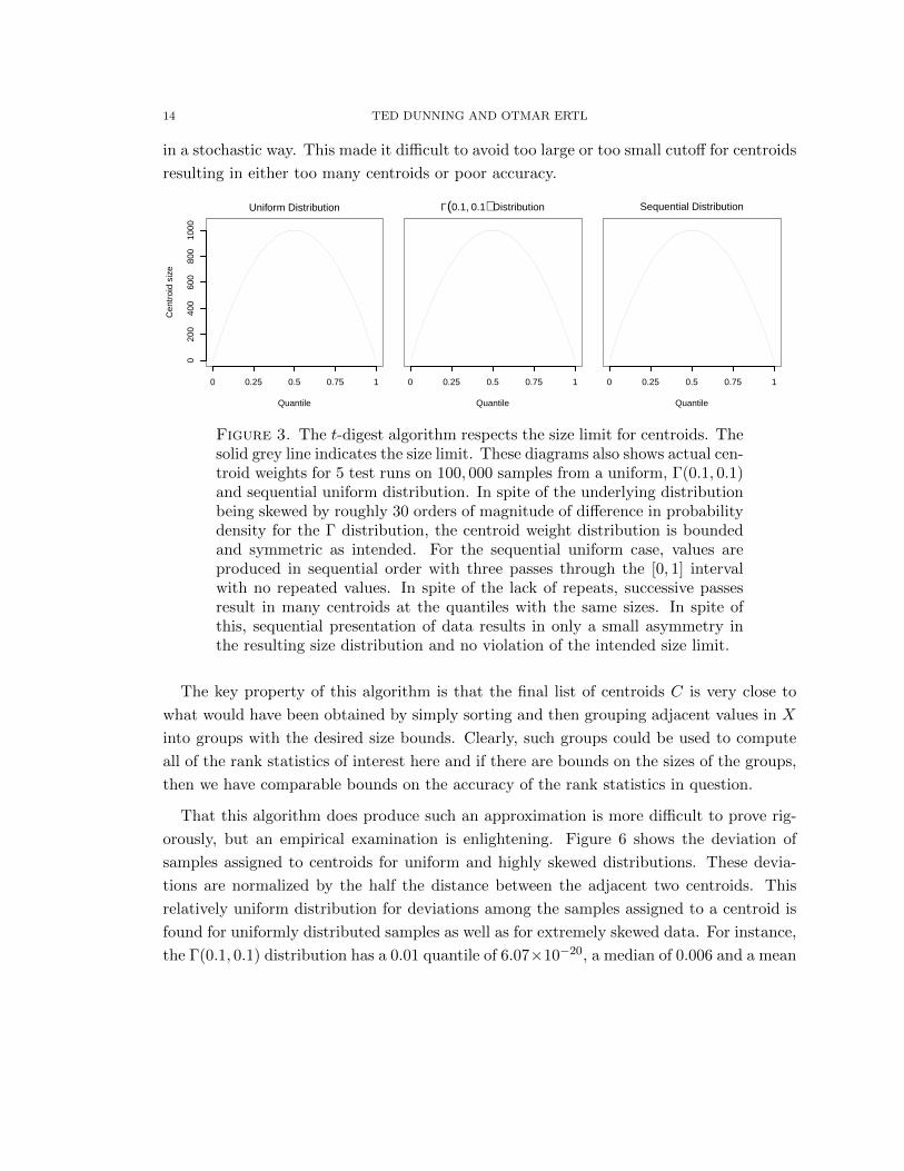
Figure 3. The t-digest algorithm respects the size limit for centroids. Thesolid grey line indicates the size limit. These diagrams also shows actual cen-troid weights for 5 test runs on 100, 000 samples from a uniform, Γ(0.1, 0.1)and sequential uniform distribution. In spite of the underlying distributionbeing skewed by roughly 30 orders of magnitude of difference in probabilitydensity for the Γ distribution, the centroid weight distribution is boundedand symmetric as intended. For the sequential uniform case, values areproduced in sequential order with three passes through the [0, 1] intervalwith no repeated values. In spite of the lack of repeats, successive passesresult in many centroids at the quantiles with the same sizes. In spite ofthis, sequential presentation of data results in only a small asymmetry inthe resulting size distribution and no violation of the intended size limit.

The key property of this algorithm is that the final list of centroids C is very close to

what would have been obtained by simply sorting and then grouping adjacent values in X

into groups with the desired size bounds. Clearly, such groups could be used to compute

all of the rank statistics of interest here and if there are bounds on the sizes of the groups,

then we have comparable bounds on the accuracy of the rank statistics in question.

That this algorithm does produce such an approximation is more difficult to prove rig-

orously, but an empirical examination is enlightening. Figure 6 shows the deviation of

samples assigned to centroids for uniform and highly skewed distributions. These devia-

tions are normalized by the half the distance between the adjacent two centroids. This

relatively uniform distribution for deviations among the samples assigned to a centroid is

found for uniformly distributed samples as well as for extremely skewed data. For instance,

the Γ(0.1, 0.1) distribution has a 0.01 quantile of 6.07×10−20, a median of 0.006 and a mean


Uniform q=0.3 ... 0.7

−1.0 −0.5 0.0 0.5 1.0

010

000

3000

0

Gamma(0.1, 0.1) q=0.3 ... 0.7

−1.0 −0.5 0.0 0.5 1.00

1000

030

000

Gamma, q=0.01

−1.0 −0.5 0.0 0.5 1.0

050

015

00

Figure 4. The deviation of samples assigned to a single centroid. Thehorizontal axis is scaled to the distance to the adjacent centroid so a valueof 0.5 is half-way between the two centroids. There are two significantobservations to be had here. The first is that relatively few points areassigned to a centroid that are beyond the midpoint to the next cluster.This bears on the accuracy of this algorithm. The second observation isthat samples are distributed relatively uniformly between the boundaries ofthe cell. This affects the interpolation method to be chosen when workingwith quantiles. The three graphs show, respectively, centroids from q ∈[0.3, 0.7] from a uniform distribution, centroids from the same range of ahighly skewed Γ(0.1, 0.1) and centroids from q ∈ [0.01, 0.015] in a Γ(0.1, 0.1)distribution. This last range is in a region where skew on the order of 1022

is found.

of 1. This means that the distribution is very skewed. In spite of this, samples assigned

to centroids near the first percentile are not noticeably skewed within the centroid. The

impact of this uniform distribution is that linear interpolation allows accuracy considerably

better than q(1− q)/δ.

2.9. Finding the cumulative distribution at a point. Algorithm 3 shows how to

compute the cumulative distribution P (x) =∫ x−∞ p(α) dα for a given value of x by summing

the contribution of uniform distributions centered at each the centroids. Each of the

centroids is assumed to extend symmetrically around the mean for half the distance to the

adjacent centroid.

For all centroids except one, this contribution will be either 0 or ci.count/N and the one

centroid which straddles the desired value of x will have a pro rata contribution somewhere

between 0 and ci.count/N . Moreover, since each centroid has count at most δN the

accuracy of q should be accurate on a scale of δ. Typically, the accuracy will be even better


due to the interpolation scheme used in the algorithm and because the largest centroids

are only for values of q near 0.5.

The empirical justification for using a uniform distribution for each centroid can be seen

by referring to again to Figure 6.

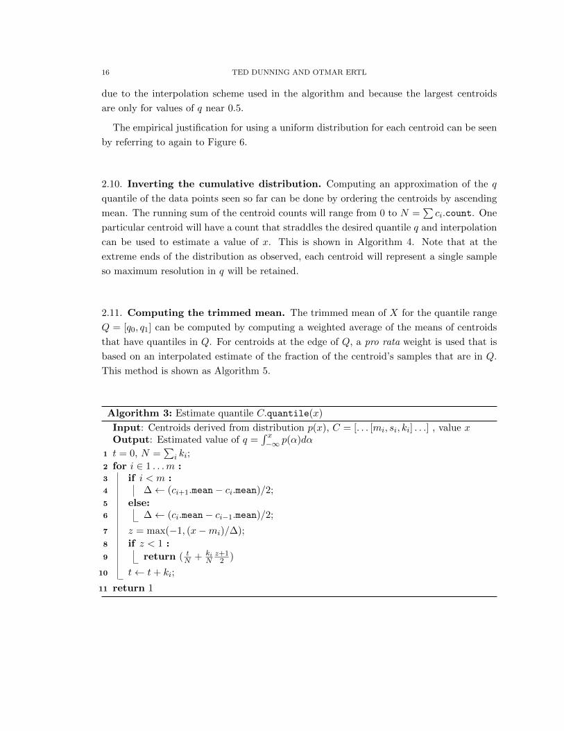
2.10. Inverting the cumulative distribution. Computing an approximation of the q

quantile of the data points seen so far can be done by ordering the centroids by ascending

mean. The running sum of the centroid counts will range from 0 to N =∑ci.count. One

particular centroid will have a count that straddles the desired quantile q and interpolation

can be used to estimate a value of x. This is shown in Algorithm 4. Note that at the

extreme ends of the distribution as observed, each centroid will represent a single sample

so maximum resolution in q will be retained.

2.11. Computing the trimmed mean. The trimmed mean of X for the quantile range

Q = [q0, q1] can be computed by computing a weighted average of the means of centroids

that have quantiles in Q. For centroids at the edge of Q, a pro rata weight is used that is

based on an interpolated estimate of the fraction of the centroid’s samples that are in Q.

This method is shown as Algorithm 5.

Algorithm 3: Estimate quantile C.quantile(x)

Input: Centroids derived from distribution p(x), C = [. . . [mi, si, ki] . . .] , value xOutput: Estimated value of q =

∫ x−∞ p(α)dα

1 t = 0, N =∑

i ki;

2 for i ∈ 1 . . .m :3 if i < m :4 ∆← (ci+1.mean− ci.mean)/2;

5 else:6 ∆← (ci.mean− ci−1.mean)/2;

7 z = max(−1, (x−mi)/∆);

8 if z < 1 :

9 return ( tN + ki

Nz+12 )

10 t← t+ ki;

11 return 1


3. Empirical Assessment

3.1. Accuracy of estimation for uniform and skewed distributions. Figure 7 shows

the error levels achieved with t-digest in estimating quantiles of 100,000 samples from a

uniform and from a skewed distribution. In these experiments δ = 0.01 was used since it

provides a good compromise between accuracy and space. There is no visible difference in

accuracy between the two underlying distributions in spite of the fact that the underlying

densities differ by more roughly 30 orders of magnitude. The accuracy shown here is

computed by comparing the computed quantiles to the actual empirical quantiles for the

sample used for testing and is shown in terms of q rather than the underlying sample value.

At extreme values of q, the actual samples are preserved as centroids with weight 1 so the

observed for these extreme values is zero relative to the original data. For the data shown

here, at q = 0.001, the maximum weight on a centroid is just above 4 and centroids in this

range have all possible weights from 1 to 4. Errors are limited to, not surprisingly, just

a few parts per million or less. For more extreme quantiles, the centroids will have fewer

samples and the results will typically be exact.

Obviously, with the relatively small numbers of samples such as are used in these ex-

periments, the accuracy of t-digests for estimating quantiles of the underlying distribution

Algorithm 4: Estimate value at given quantile C.icdf(q)

Input: Centroids derived from distribution p(x), C = [c1 . . . cm] , value qOutput: Estimated value x such that q =

∫ x−∞ p(α)dα

1 t = 0, q ← q∑ci.count;

2 for i ∈ 1 . . .m :3 ki = ci.count;

4 mi = ci.mean;

5 if q < t+ ki :6 if i = 1 :7 ∆← (ci+1.mean− ci.mean);

8 elif i = m :9 ∆← (ci.mean− ci−1.mean);

10 else:11 ∆← (ci+1.mean− ci−1.mean)/2;

12 return mi +(q−tki− 1

2

)∆

13 t← t+ ki

14 return cm.mean


cannot be better than the accuracy of these estimates computed using the sample data

points themselves. For the experiments here, the errors due to sampling completely domi-

nate the errors introduced by t-digests, especially at extreme values of q. For much larger

sample sets of billions of samples or more, this would be less true and the errors shown

here would represent the accuracy of approximating the underlying distribution.

Algorithm 5: Estimate trimmed mean. Note how centroids at the boundary areincluded on a pro rata basis.

Input: Centroids derived from distribution p(x), C = [. . . [mi, si, ki] . . .] , limit valuesq0, q2

Output: Estimate of mean of values x ∈ [q0, q1]1 s = 0, k = 0;

2 t = 0, q1 ← q1∑ki, q1 ← q1

∑ki;

3 for i ∈ 1 . . .m :4 ki = ci.count;

5 if q1 < t+ ki :6 if i > 1 :7 ∆← (ci+1.mean− ci−1.mean)/2;

8 elif i < m :9 ∆← (ci+1.mean− ci.mean);

10 else:11 ∆← (ci.mean− ci−1.mean);

12 η =(q−tki− 1

2

)∆;

13 s← s+ η ki ci.mean;

14 k ← k + η ki;

15 if q2 < t+ ki :16 if i > 1 :17 ∆← (ci+1.mean− ci−1.mean)/2;

18 elif i < m :19 ∆← (ci+1.mean− ci.mean);

20 else:21 ∆← (ci.mean− ci−1.mean);

22 η =(12 −

q−tki

)∆;

23 s← s− η ki ci.mean;

24 k ← k − η ki;25 t← t+ ki

26 return s/k


0.001 0.01 0.1 0.5 0.9 0.99 0.999

−20

00−

1000

010

0020

00

Uniform

Quantile (q)

Qua

ntile

err

or (

ppm

)

0.001 0.01 0.1 0.5 0.9 0.99 0.999

Γ(0.1, 0.1)

Quantile (q)

Figure 5. The absolute error of the estimate of the cumulative distributionfunction q =

∫ x−∞ p(α) dα for the uniform and Γ distribution for 5 runs,

each with 100,000 data points. As can be seen, the error is dramaticallydecreased for very high or very low quantiles (to a few parts per million).The precision setting used here, 1/δ = 100, would result in uniform error of10,000 ppm without adaptive bin sizing and interpolation.

It should be noted that using a Q-Digest implemented with long integers is only able

to store data with no more than 20 significant decimal figures. The implementation in

stream-lib only retains 48 bits of significants, allowing only about 16 significant figures.

This means that such a Q-digest would be inherently unable to even estimate the quantiles

of the Γ distribution tested here.

3.2. Persisting t-digests. For the accuracy setting and test data used in these experi-

ments, the t-digest contained 820−860 centroids. The results of t-digest can thus be stored

by storing this many centroid means and weights. If centroids are kept as double precision

floating point numbers and counts kept as 4-byte integers, the t-digest resulting from from

the accuracy tests described here would require about 10 kilobytes of storage for any of

the distributions tested.

This size can be substantially decreased, however. One simple option is to store differ-

ences between centroid means and to use a variable byte encoding such as zig-zag encoding

to store the cluster size. The differences between successive means are at least three orders


of magnitude smaller than the means themselves so using single precision floating point

to store these differences can allow the t-digest from the tests described here to be stored

in about 4.6 kilobytes while still regaining nearly 10 significant figures of accuracy in the

means. This is roughly equivalent to the precision possible with a Q-digest operating on

32 bit integers, but the dynamic range of t-digests will be considerably higher and the

accuracy is considerably better.

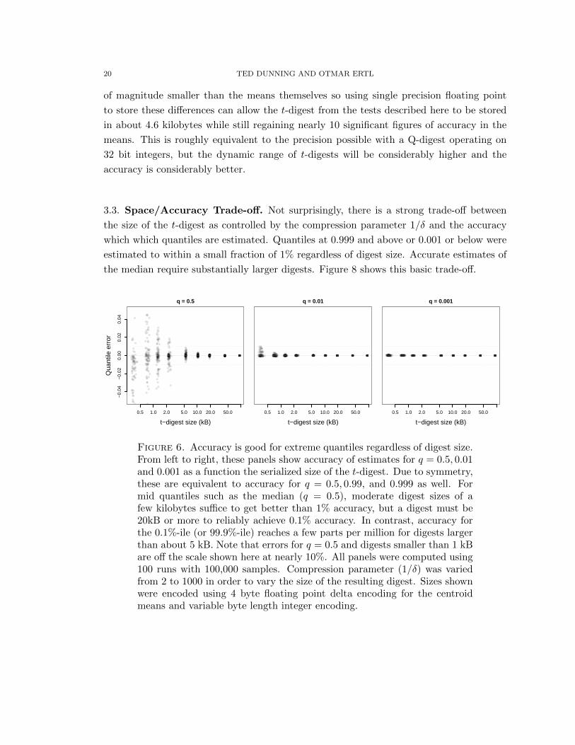
3.3. Space/Accuracy Trade-off. Not surprisingly, there is a strong trade-off between

the size of the t-digest as controlled by the compression parameter 1/δ and the accuracy

which which quantiles are estimated. Quantiles at 0.999 and above or 0.001 or below were

estimated to within a small fraction of 1% regardless of digest size. Accurate estimates of

the median require substantially larger digests. Figure 8 shows this basic trade-off.

0.5 1.0 2.0 5.0 10.0 20.0 50.0

q = 0.5

t−digest size (kB)

Qua

ntile

err

or

−0.

04−

0.02

0.00

0.02

0.04

0.5 1.0 2.0 5.0 10.0 20.0 50.0

q = 0.01


Qua

ntile

err

or

0.5 1.0 2.0 5.0 10.0 20.0 50.0

q = 0.001


Qua

ntile

err

or

Figure 6. Accuracy is good for extreme quantiles regardless of digest size.From left to right, these panels show accuracy of estimates for q = 0.5, 0.01and 0.001 as a function the serialized size of the t-digest. Due to symmetry,these are equivalent to accuracy for q = 0.5, 0.99, and 0.999 as well. Formid quantiles such as the median (q = 0.5), moderate digest sizes of afew kilobytes suffice to get better than 1% accuracy, but a digest must be20kB or more to reliably achieve 0.1% accuracy. In contrast, accuracy forthe 0.1%-ile (or 99.9%-ile) reaches a few parts per million for digests largerthan about 5 kB. Note that errors for q = 0.5 and digests smaller than 1 kBare off the scale shown here at nearly 10%. All panels were computed using100 runs with 100,000 samples. Compression parameter (1/δ) was variedfrom 2 to 1000 in order to vary the size of the resulting digest. Sizes shownwere encoded using 4 byte floating point delta encoding for the centroidmeans and variable byte length integer encoding.


The size of the resulting digest depends strongly on the compression parameter 1/δ as

shown in the left panel of Figure 9. Size of the digest also grows roughly with the log of the

number of samples observed, at least in the range of 10,000 to 10,000,000 samples shown

in the right panel of Figure 9.

2 5 10 20 50 100 500

1 δ

Siz

e (k

B)

0.1

110

100

10M samples10k samples

05

1015

20

1 δ = 100

Samples (x1000)

Siz

e (k

B)

10 100 1000 10,000

Figure 7. Size of the digest scales sub-linearly with compression parame-ter (α ≈ 0.7 . . . 0.9) for fixed number of points. Size scales approximatelylogarithmically with number of points for fixed compression parameter. Thepanel on the right is for 1/δ = 100. The dashed lines show best-fit log-linearmodels. In addition, the right panel shows the memory size required for theGK01 algorithm if 6 specific quantiles are desired.

3.4. Computing t-digests in parallel. With large scale computations, it is important to

be able to compute aggregates like the t-digest on portions of the input and then combine

those aggregates.

For example, in a map-reduce framework such as Hadoop, a combiner function can

compute the t-digest for the output of each mapper and a single reducer can be used to

compute the t-digest for the entire data set.

Another example can be found in certain databases such as Couchbase or Druid which

maintain tree structured indices and allow the programmer to specify that particular ag-

gregates of the data being stored can be kept at interior nodes of the index. The benefit of

this is that aggregation can be done almost instantaneously over any contiguous sub-range

of the index. The cost is quite modest with only a O(log(N)) total increase in effort over

keeping a running aggregate of all data. In many practical cases, the tree can contain only


two or three levels and still provide fast enough response. For instance, if it is desired to

be able to compute quantiles for any period up to years in 30 second increments, simply

keeping higher level t-digests at the level of 30 seconds and days is likely to be satisfactory

because at most about 10,000 digests are likely to need merging even for particularly odd

intervals. If almost all queries over intervals longer than a few weeks are day aligned, the

number of digests that must be merged drops to a few thousand.

−1

00

00

−5

00

00

50

00

10

00

0

Quantile (q)

Err

or

in q

ua

ntile

(p

pm

)

−1

00

00

−5

00

00

50

00

10

00

0

0.001 0.1 0.2 0.3 0.5

DirectMerged

1 δ = 50

5 parts

Quantile (q)

0.001 0.01 0.1 0.2 0.3 0.5

DirectMerged

1 δ = 50

20 parts

Quantile (q)

0.001 0.01 0.1 0.2 0.3 0.5

DirectMerged

1 δ = 50

100 parts

Figure 8. Accuracy of a t-digest accumulated directly is nearly the sameas when the digest is computed by combining digests from 20 or 100 equalsized portions of the data. Repeated runs of this test occasionally show thesituation seen in the left panel where the accuracy for digests formed from 5partial digests show slightly worse accuracy than the non-subdivided case.This sub-aggregation property allows efficient use of the tdigest in map-reduce and database applications. Of particular interest is the fact thataccuracy actually improves when the input data is broken in to many partsas is shown in the right hand panel. All panels were computed by 40 rep-etitions of aggregating 100,000 values. Accuracy for directly accumulateddigests is shown on the left of each pair with the white bar and the digestof digest accuracy is shown on the right of each pair by the dark gray bar.

Merging t-digests can be done many ways. The algorithm whose results are shown here

consisted of simply making a list of all centroids from the t-digests being merged, shuffling

that list, and then adding these centroids, preserving their weights, to a new t-digest.

3.5. Comparison with Q-digest. The prototype implementation of the t-digest com-

pletely dominates the implementation of the Q-digest from the popular stream-lib package


[Thi] when size of the resulting digest is controlled. This is shown in Figure 11. In the

left panel, the relationship between the effect of the compression parameter for Q-digest is

compared to the similar parameter 1/δ for the t-digest. For the same value of compression

parameter, the sizes of the two digests is always within a factor of 2 for practical uses. The

middle and right panel show accuracies for uniform and Γ distributions.

t−digest (bytes)

Q−

dige

st (

byte

s)

100 300 1K 3K 10K 30K 100K

100

300

1K3K

10K

30K

100K

2

5

10

20

50

100

200

500

1000

2000

1 δ

Quantile

Qua

ntile

err

or (

ppm

)

0.001 0.1 0.5 0.9 0.99

−10

000

050

0015

000

Q−digestt−digest

Uniform1 δ = 50

020

000

4000

060

000

8000

0

Quantile

Qua

ntile

err

or (

ppm

)

020

000

4000

060

000

8000

0

0.001 0.1 0.5 0.9 0.99

Q−digestt−digest

Γ(0.1, 0.1)1 δ = 50

Figure 9. The left panel shows the size of a serialized Q-digest versus thesize of a serialized t-digest for various values of 1/δ from 2 to 100,000. Thesizes for the two kinds of digest are within a factor of 2 for all compressionlevels. The middle and right panels show the accuracy for a particularsetting of 1/δ for Q-digest and t-digest. For each quantile, the Q-digestaccuracy is shown as the left bar in a pair and the t-digest accuracy is shownas the right bar in a pair. Note that the vertical scale in these diagramsare one or two orders of magnitude larger than in the previous accuracygraphs and that in all cases, the accuracy of the t-digest is dramaticallybetter than that of the Q-digest even though the serialized size of the eachis within 10% of the other. Note that the errors in the right hand panelare systematic quantization errors introduced by the use of integers in theQ-digest algorithm. Any distribution with very large dynamic range willshow the same problems.

As expected, the t-digest has very good accuracy for extreme quantiles while the Q-

digest has constant error across the range. Interestingly, the accuracy of the Q-digest is at

best roughly an order of magnitude worse than the accuracy of the t-digest even. At worse,

with extreme values of q, accuracy is several orders of magnitude worse. This situation

is even worse with a highly skewed distribution such as with the Γ(0.1, 0.1) shown in the

right panel. Here, the very high dynamic range introduces severe quantization errors into

the results. This quantization is inherent in the use of integers in the Q-digest.


For higher compression parameter values, the size of the Q-digest becomes up to two

times smaller than the t-digest, but no improvement in the error rates is observed.

3.6. Speed. The current implementation has been primarily optimized for ease of devel-

opment, not execution speed. As it is, running on a single core of a 2.3 GHz Intel Core i5,

it typically takes 2-3 microseconds to process each point after JIT optimization has come

into effect. It is to be expected that a substantial improvement in speed could be had by

profiling and cleaning up the prototype code.

4. Conclusion

The t-digest is a novel algorithm that dominates the previously state-of-the-art Q-digest

in terms of accuracy and size. The t-digest provides accurate on-line estimates of a variety

of of rank-based statistics including quantiles and trimmed mean. The algorithm is simple

and empirically demonstrated to exhibit accuracy as predicted on theoretical grounds. It

is also suitable for parallel applications. Moreover, the t-digest algorithm is inherently

on-line while the Q-digest is an on-line adaptation of an off-line algorithm.

The t-digest algorithm is available in the form of an open source, well-tested implemen-

tation from the author. It has already been adopted by the Apache Mahout and stream-lib

projects and is likely to be adopted by other projects as well.

References

[CLP00] Fei Chen, Diane Lambert, and Jos C. Pinheiro. Incremental quantile estimation for massive

tracking. In In Proceedings of KDD, pages 516–522, 2000.

[GK01] Michael Greenwald and Sanjeev Khanna. Space-efficient online computation of quantile sum-

maries. In In SIGMOD, pages 58–66, 2001.

[Knu98] Donald E. Knuth. The Art of Computer Programming, volume 2: Seminumerical Algorithms,

page 232. Addison-Wesley, Boston, 3 edition, 1998.

[Lin] LinkedIn. Datafu: Hadoop library for large-scale data processing. https://github.com/

linkedin/datafu/. [Online; accessed 20-December-2013].

[MP80] J.I. Munro and M.S. Paterson. Selection and sorting with limited storage. Theoretical Computer

Science, 12(3):315 – 323, 1980.

[PDGQ05] Rob Pike, Sean Dorward, Robert Griesemer, and Sean Quinlan. Interpreting the data: Parallel

analysis with sawzall. Sci. Program., 13(4):277–298, October 2005.

[SBAS04] Nisheeth Shrivastava, Chiranjeeb Buragohain, Divyakant Agrawal, and Subhash Suri. Medians

and beyond: New aggregation techniques for sensor networks. pages 239–249. ACM Press, 2004.


[Thi] Add This. Algorithms for calculating variance, online algorithm. https://github.com/

addthis/stream-lib. [Online; accessed 28-November-2013].

[Wel62] B. P. Welford. Note on a method for calculating corrected sums of squares and products. Tech-

nometrics, pages 419–420, 1962.

[Wik] Wikipedia. Algorithms for calculating variance, online algorithm. http://en.wikipedia.

org/wiki/Algorithms_for_calculating_variance#Online_algorithm. [Online; accessed 19-

October-2013].

Ted Dunning, MapR Technologies, Inc, San Jose, CA

E-mail address: [email protected]

E-mail address: [email protected]

computing extremely accurate quantiles using t-digests · computing extremely accurate quantiles...

Documents