continuous random variables: quantiles, expected value ... · continuous random variables:...

ContinuousRandom Variables:

Quantiles,Expected Value,

and Variance

Will Landau

Quantiles

Expected Value

Variance

Functions ofrandom variables

Continuous Random Variables: Quantiles,Expected Value, and Variance

Will Landau

Iowa State University

Feb 26, 2013

© Will Landau Iowa State University Feb 26, 2013 1 / 27



and Variance

Will Landau

Quantiles

Expected Value

Variance


Outline

Quantiles

Expected Value

Variance

Functions of random variables




and Variance

Will Landau

Quantiles

Expected Value

Variance


Quantiles of continuous distributions

I The p-quantile of a random variable, X, is the number,Q(p), such that:

P(X ≤ Q(p)) = p

I In terms of the cumulative distribution function (cdf):

F (Q(p)) = p

Q(p) = F−1(p)




and Variance

Will Landau

Quantiles

Expected Value

Variance


ExampleI Let Y be the time delay (s) between a 60 Hz AC circuit and the

movement of a motor on a different circuit.

f (y) =

{60 0 < y < 1

60

0 otherwise

I Q(0.95) :

0.95 = P(Y ≤ Q(0.95)) =

∫ Q(0.95)

−∞f (y)dy

=

∫ 0

−∞0dx +

∫ Q(0.95)

060dy = 0 + (60|Q(0.95)

0

= 60Q(0.95)

Q(0.95) =0.95

60=

19

1200≈ 0.0158

Interpretation: on average, 95% of the time delays will be below 0.0158seconds.




and Variance

Will Landau

Quantiles

Expected Value

Variance


ExampleI You can also calculate quantiles directly from the cdf:

F (y) =

0 y ≤ 0

60y 0 < y ≤ 160

1 y > 160

I Q(0.25):

0.25 = P(Y ≤ Q(0.25)) = F (Q(0.25))

= 60 · Q(0.25)

Hence:

Q(0.25) =0.25

60=

1

240≈ 0.00417

Interpretation: on average, 25% of the time delays willbe below 0.00417 seconds.




and Variance

Will Landau

Quantiles

Expected Value

Variance


Your turn: calculating quantiles

I T ∼ Exp(α = 1/2):

f (t) =

{0 t ≤ 0

2e−2t t ≥ 0F (t)

{0 t < 0

1 − e−2t t ≥ 0

I Find:

1. Q(0.05)2. Q(0.5)3. Q(p) for some p with 0 ≤ p ≤ 1




and Variance

Will Landau

Quantiles

Expected Value

Variance


Answers: calculating quantiles

1. Q(0.05):

0.05 = P(T ≤ Q(0.05)) = F (Q(0.05)) = 1 − e−2Q(0.05)

0.95 = e−2Q(0.05)

log(0.95) = −2Q(0.05)

Q(0.05) =log(0.95)

−2≈ 0.0256

2. Q(0.5):

0.5 = P(T ≤ Q(0.5)) = F (Q(0.5)) = 1 − e−2Q(0.5)

0.5 = e−2Q(0.5)

log(0.5) = −2Q(0.5)

Q(0.5) =log(0.5)

−2≈ 0.347




and Variance

Will Landau

Quantiles

Expected Value

Variance


Answers: calculating quantiles

3. Q(p)

p = P(T ≤ Q(p)) = F (Q(p)) = 1 − e−2Q(p)

1 − p = e−2Q(p)

log(1 − p) = −2Q(p)

Q(p) =log(1 − p)

−2




and Variance

Will Landau

Quantiles

Expected Value

Variance


Outline

Quantiles

Expected Value

Variance





and Variance

Will Landau

Quantiles

Expected Value

Variance


Expected value

I The expected value of a continuous random variable is:

E (X ) =

∫ ∞−∞

x · f (x)dx

I As with continuous random variables, E (X ) (oftendenoted by µ) is the mean of X , a measure of center.




and Variance

Will Landau

Quantiles

Expected Value

Variance


Example: time delay, Y

f (y) =

{60 0 ≤ y ≤ 1

60

0 otherwise

E (Y ) =

∫ ∞−∞

y · f (y)dy

=

∫ 0

−∞y · 0dy +

∫ 1/60

0y · 60dy +

∫ ∞1/60

y · 0dy

= 0 +

(y2

2· 60

)1/60

0

+ 0

=1

2

(1

60

)2

· 60 =1

120




and Variance

Will Landau

Quantiles

Expected Value

Variance


E(X) is the “center of mass” of a distribution




and Variance

Will Landau

Quantiles

Expected Value

Variance


Your turn: calculate E(X )

f (x) =

{0 x < 01αe−x/α x ≥ 0

1. X ∼ Exp(3)

2. X ∼ Exp(α)




and Variance

Will Landau

Quantiles

Expected Value

Variance


Answers: Calculate E(X )1. X ∼ Exp(3):

E(X ) =

∫ ∞−∞

x · f (x)dx

=

∫ 0

−∞x · 0dx +

∫ ∞0

x ·1

3e−x/3dx

integration by parts:

= 0 +(x(−e−x/3)

)∞0−∫ ∞

0(−e−x/3)dx

=(−∞e−∞/3 + 0e−0/3

)+

∫ ∞0

e−x/3dx

= 0 +(−3e−x/3

)∞0

=(−3e−∞/3 + 3e−0/3

)= 3

2. Similarly, E(X) = α when X ∼ Exp(α).




and Variance

Will Landau

Quantiles

Expected Value

Variance


Example: waiting time for the next student to arrive at the library

I From 12:00 to 12:10 PM, about 12.5 students per minute enter onaverage.

I Hence, the average waiting time for the next student is 112.5

= 0.08minutes for the next student.

I Let T ∼ Exp(0.08) be the time until the next student arrives.

I P(wait is more than 10 seconds) =

P (T > 1/6) = 1− F (1/6) = 1−(

1− e(−0.08·1/6))

= 0.12




and Variance

Will Landau

Quantiles

Expected Value

Variance


Outline

Quantiles

Expected Value

Variance





and Variance

Will Landau

Quantiles

Expected Value

Variance


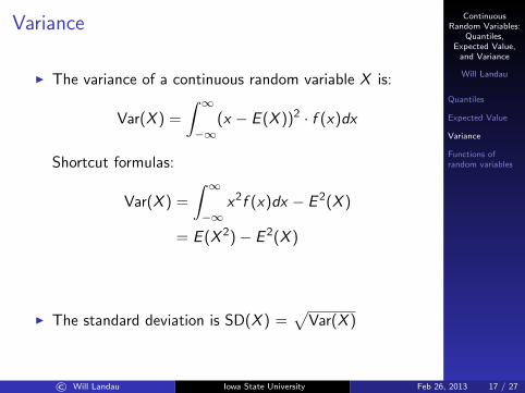
Variance

I The variance of a continuous random variable X is:

Var(X ) =

∫ ∞−∞

(x − E (X ))2 · f (x)dx

Shortcut formulas:

Var(X ) =

∫ ∞−∞

x2f (x)dx − E 2(X )

= E (X 2) − E 2(X )

I The standard deviation is SD(X ) =√

Var(X )




and Variance

Will Landau

Quantiles

Expected Value

Variance


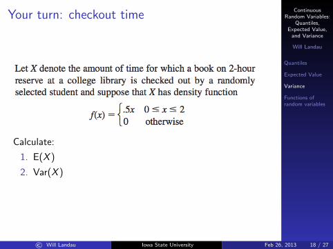
Your turn: checkout time

Calculate:

1. E(X )

2. Var(X )




and Variance

Will Landau

Quantiles

Expected Value

Variance


Answers: checkout time

1.

E (X ) =

∫ ∞−∞

x · f (x)dx =

∫ 2

0

x · 1

2xdx

=1

2

∫ 2

0

x2dx =

(x3

6

)2

0

=8

6≈ 1.333

2.

E (X 2) =

∫ ∞−∞

x2f (x)dx =

∫ 2

0

x2 1

2xdx =

1

2

∫ 2

0

x3dx =

(x4

8

)2

0

= 2

Var(X ) = E (X 2) − E 2(X ) = 2

(8

6

)2

=2

9




and Variance

Will Landau

Quantiles

Expected Value

Variance


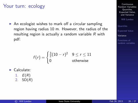
Your turn: ecology

I An ecologist wishes to mark off a circular samplingregion having radius 10 m. However, the radius of theresulting region is actually a random variable R withpdf:

f (r) =

{32 (10 − r)2 9 ≤ r ≤ 11

0 otherwise

I Calculate:

1. E (R)2. SD(R)




and Variance

Will Landau

Quantiles

Expected Value

Variance


Answers: ecology

1.

E(R) =

∫ ∞−∞

r · f (r)dr

=

∫ 11

9r ·

3

2(10− r)2dr

=

∫ 11

9

(3

2r3 − 30r2 + 150r

)dr

=

(3

8r3 − 10r3 + 75r2

)11

9

=

(3

8(11)3 − 10(11)3 + 75(11)2

)−(

3

893 − 10(9)3 + 75(9)2

)= 10




and Variance

Will Landau

Quantiles

Expected Value

Variance


Answers: ecology

2.

E(R2) =

∫ ∞−∞

r2 · f (r)dr

=

∫ 11

9r2 ·

3

2(10− r)2dr

=

∫ 11

9

(3

2r4 − 30r3 + 150r2

)dr

=

(3

10r5 −

15

2r4 + 50r3

)11

9

=

(3

10(11)5 −

15

2(11)4 + 50(11)3

)−(

3

10(9)5 −

15

2(9)4 + 50(9)3

)=

503

5= 100.6

Var(R) = E(R2)− E2(R) =503

5− 102 =

3

5= 0.6

SD(R) =√

Var(R) =√

0.6 ≈ 2.449




and Variance

Will Landau

Quantiles

Expected Value

Variance


Outline

Quantiles

Expected Value

Variance





and Variance

Will Landau

Quantiles

Expected Value

Variance


Expectation of a function of a random variableI Why does E (X 2) =

∫∞−∞ x2 · f (x)dx?

I It turns out that for any function g of a randomvariable:

E (g(X )) =

∫ ∞−∞

g(x) · f (x)dx

I Hence:

E (X 2) =

∫ ∞−∞

x2 · f (x)dx

if we take g(X ) = X 2.I In the ecology example, the expected area of the

circular sampling region is:

E (πR2) =

∫ ∞−∞

πr2 · f (r)dr

where πR2 = g(R) is the sampling area.




and Variance

Will Landau

Quantiles

Expected Value

Variance


Expectation of a linear function of X

I For constants a and b:

E (aX + b) =

∫ ∞−∞

(ax + b) · f (x)dx

= a

∫ ∞−∞

x · f (x)dx︸︷︷︸E(X )

+b

∫ ∞−∞

f (x)dx︸︷︷︸1

= aE (X ) + b

I Example: the expected diameter of the ecologist’s samplingregion is:

E (2 · R + 0) = 2 · E (R) + 0 = 2 · 10 = 20




and Variance

Will Landau

Quantiles

Expected Value

Variance


Variance of a linear function of X

I For constants a and b:

Var(aX + b) = E ((aX + b)2) − E 2(aX + b)

= E (a2X 2 + abX + b2) − (aE (X ) + b)2

= (a2E (X 2) + abE (X ) + b2)

− (a2E 2(X ) + abE (X ) + b2)

= a2(E (X 2) − E 2(X ))

= a2Var(X )

I Example: the variance of the diameter of the ecologist’ssampling region is:

Var(2 · R + 0) = 4Var(R) = 4 · 503

5=

2012

5




and Variance

Will Landau

Quantiles

Expected Value

Variance


StandardizationI Standardization: converting a random variable X into another random

variable Z by subtracting the mean and dividing by the standarddeviation:

Z =X − E(X )

SD(X )

I Z has mean 0:

E(Z) = E

(X − E(X )

SD(X )

)= E

(1

SD(X )· X −

E(X )

SD(X )

)=

1

SD(X )· E(X )−

E(X )

SD(X )= 0

I Z has variance (and standard deviation) 1:

Var(Z) = Var

(X − E(X )

SD(X )

)= Var

(1

SD(X )· X −

E(X )

SD(X )

)=

1

SD2(X )Var(X ) = Var(X )

1

Var(X )= 1


continuous random variables: quantiles, expected value ... · continuous random variables:...

Documents