computerized tomography - unigrazphysik.uni-graz.at/~uxh/diploma/fliesser15.pdf · computerized...

Karl-Franzens-Universitat Graz

Bachelorarbeit

Computerized Tomography

Verfasserin: Katharina Fließer

Betreuer: Ao. Univ.-Prof. Dr. Ulrich Hohenester

Datum: 28.01.2015

28.01.2015 Computerized Tomography Katharina Fließer

Contents

1 Introduction 2

2 Computerized Tomography 4

3 Radon transformation 7

4 Image Reconstruction 104.1 Iterative Reconstruction . . . . . . . . . . . . . . . . . . . . . . . . . . . . 104.2 Back projection . . . . . . . . . . . . . . . . . . . . . . . . . . . . . . . . . 144.3 Central Slice Theorem . . . . . . . . . . . . . . . . . . . . . . . . . . . . . 154.4 Filtered back projection . . . . . . . . . . . . . . . . . . . . . . . . . . . . 17

4.4.1 Noise in Computerized Thomography . . . . . . . . . . . . . . . . . 194.4.2 Filtering . . . . . . . . . . . . . . . . . . . . . . . . . . . . . . . . . 20

5 Discrete Problem 245.1 Sampling . . . . . . . . . . . . . . . . . . . . . . . . . . . . . . . . . . . . . 245.2 Discrete Functions and Filters . . . . . . . . . . . . . . . . . . . . . . . . . 25

6 Conclusions 29

1/ 30


1 Introduction

Computerized Tomography, short CT, or also called Computed Axial Tomopraphy (CAT),is a method used in medicin to generate images of the interior of the body. As a differ-ence to conventional radiography, where the result is a two dimensional ”photograph” ofa body’s inside, CT scans yield a three−dimensional reconstruction of the body and itsinterior.CT imaging works through composition of slices of anatomy, which have been individuallyconsidered. Thus CT scanning also allows the visualization of a single slice of anatomyat any oblique angle. Hence CT imaging is a lot more flexible than standard radiographyand allows a more thorough examination of a body’s inside and makes it easier to spotdefects.Modern X-ray detectors allow the observation of contrasts of the order of 2%, accordingto [2]. This enables to visualize the anatomy of the heart, air−filled tracheas, or blood invessels and other soft tissue details which can not be seen with conventional radiography.

Whereas the word ”Tomography” is derived from the Greek words ”tomos”, meaning”slice” or ”section”, and ”graphia”, meaning ”describing”, the word ”Computerized”indicates the need for a computer to produce an image. As a consequence, the imagereconstruction methods used in Computerized Tomography have to be checked for theirfeasibility and efficiency on a computer. Though there are a couple of methods that wouldbe suitable for the computerized image reconstruction, the currently common method inmedical practice is based on the Radon transform invented by the Austrian mathemati-cian Johann Radon. The Radon transform was first published in Radon’s paper” Uber die Bestimmung von Funktionen durch ihre Integralwerte langs gewisserMannigfaltigkeiten” in 1917 (see reference [8]).

It was not until the improvement of the computer technology in the 1960’s and 70’sthat Computerized Tomography itself could be invented.In 1964 the south African physicist Allen M. Cormack published work describing how toascertain the density of individual points of a volume by rotating an X-ray tube aroundthe object and producing images after successive 7.5o of rotations.The first computer tomograph was invented by the English engineer Godfrey N. Hounsfieldin 1971. Both, Housefield and Cormack, received the Nobel Prize for medicine in 1979for their contributions inventing CT scanners usable in medical practice.

Since its development Computerized Tomography has made an enormous progress. In1968 the measurement took up to nine hours and the image reconstruction furthermoretwo and a half. The image of a brain merely allowed a differentiation between gray andwhite brain matter.Nowadays CT examinations normally take 30 seconds to three minutes. Figure 1 com-pares the first clinical CT scan made during the early 1970’s with a CT scan from 1994.

2/ 30


Figure 1: On the left: the polaroid image of the first clinical CT scan, on the right: image of a brainmade in 1994 with a more advanced computer tomograph. The images are taken from Thomas A.M.K.,Banerjee A.K., Busch U., Classic Papers in Modern Diagnostic Radiology. ( Springer Verlag, Berlin,2005)

The invention of Computerized Tomography has been an enormous step forward inmedical diagnostic, and the method has become an indispensable part of modern medicine.Even though there are other competitive methods like MRT and ultrasonics, most radio-logical images are still produced by CT (see reference [7]).

3/ 30


2 Computerized Tomography

Computerized Tomography works with X-rays. The typical energy of such an X-ray isin the range of 100 eV to 100 keV. If a X-ray beam passes through a material part ofits energy will be absorbed. Inelastic processes which lead to absorption and to a loss ofenergy are photon absorption and Compton scattering. There are also elastic processeslike Thomson- or Rayleigh scattering.In medical imaging the materials of interest are tissues like muscle, bone or blood. Eachof these tissues has a different ability to absorb X-ray energy. So if we know how muchenergy gets lost within a tissue we can tell of what kind of material it is made of.But what if an X-ray is send through a human thorax? Within the human body there isnot only one single kind of tissue. An X-ray sent through a human chest would not onlypass through bone, but also through muscle, blood and even air within the lungs. Eachof these materials absorbs a specific part of the initial energy of the passing X-ray. Whatwe can measure is the energy on the other side of the hole thorax.So how can we reconstruct which materials have been involved, and create an image ofthe inside of a body or any other object?For a closer inspection, we first try to find a way to better describe the energy loss ofthe X-ray beam. A convenient way is to use the beams intensity (or energy flux density),which is its energy per unit time and unit area. We will call the X-rays initial intensity,its intensity before it has past through any material, I0. In Computerized TomographyI0 is a known parameter.To describe some materials ability to absorb energy, we use the linear attenuation coef-ficient µ. For example, the linear attenuation coefficents for the energy spectrum of atypical diagnostic X-ray beam for air, bone, muscle and blood are, according to [2].

µair = 0

µbone = 0.48cm−1

µmuscle = 0.18cm−1

µblood = 0.178cm−1.

Knowing the initial intensity I0, the distance x travelled by the X-ray and the attenuationcoefficient µ of the material the X-ray passed through, we can compute the new intensityof the X-ray emerging the material as I = I0exp(−µx). If the X-ray beam passes througha row of different materials with different linear attenuation coefficients µ1, µ2, µ3... wecompute µi = µ1 + µ2 + µ3 + ... and our intensity becomes

I = I0exp(−µix). (1)

Equation (1) is called the Lambert-Beer law. It tells us that the intensity of an X-raywithin a material decreases exponentially with the materials attenuation coefficient andthe distance travelled.

4/ 30


Figure 2: Intensity of an X-ray beam passing through a tissue with four different linear attenuationcoefficients µ1, µ2, µ3, µ4. Figure taken from Edwin L. Dove, Notes on Computerized Tomography (Insti-tutionen for medicinsk, 2001)

In practice we know the initial intensity I0 of the X-ray beam and detect the intensityI of the X-ray emerged. What we do not know yet are the individual components of thesample the X-ray passed and their individual attenuation coefficients.To reassemble an image of the inside of a sample, it takes more information than weget by a single X-ray beam sent through along one straight line. What is necessary isto scan the sample from a lot of different directions. In Computerized Tomography theradiation source scans the object linearly along a fixed angle θ, and afterwards rotatesaround the sample by a small angle ∆θ. This process is repeated until the rotation of180o is complete.

Figure 3: Parallel beam and angular scanning. Figure taken from Edwin L. Dove, Notes on ComputerizedTomography (Institutionen for medicinsk, 2001)

What is done during the measurement can be imagined like smearing through wetpaint. Imagine three dots of different coloured wet paint. One yellow, one blue and onered. The information you get in CT by detecting the intensity I can be compared withknowing the colors you get if you smear the coloured dots. For red and blue you getviolet, blue and yellow give green, yellow and red become orange and by mixing all threeof them you get brown.

In this example it is relatively easy to reconstruct which colours have been involvedjust by knowing the basics of chromatics and ”back projecting” orange to red mixed withyellow. It also only takes a few projections to reassemble how they might have beenarranged.To derive the unknown attenuation coefficients inside a sample in Computerized Tomog-

5/ 30


Figure 4: Color−example

raphy, we have to figure out how best to back project our detected intensities. But firstwe have to take a closer look on the projection we want to invert, and our next section isdedicated to the Radon transformation.In Section 5.1 we will investigate in more detail how many views are needed to reconstructthe original image best as possible.

6/ 30


3 Radon transformation

If we switch from discrete attenuation coefficients µi to a continuous distribution than thetwo dimensional function f(x, y) represents the linear attenuation coefficient of a tissue.The angle between the X-ray beam penetrating the tissue and the x− axis is denoted asθ.

Figure 5: Coordinatesysthem for the parallel beam geomety. Figure taken from Edwin L. Dove, Noteson Computerized Tomography (Institutionen for medicinsk, 2001)

By rotating the coordinates (x, y) clockwise over θ, as is done in Computerized Tomog-raphy, a new coordinate system (t, θ) is created. The change from (x, y) to (t, θ) obeysthe transformation formulae:

�x

y

�=

�cos θ − sin θsin θ cos θ

� �t

s

�(2)

or �t

s

�=

�cos θ sin θ− sin θ cos θ

� �x

y

�(3)

We use equation (1), the Lambert-Beer law, and compute the intensity detected for afixed angle θ

Iθ(t) = I0exp[−�

s

f(x, y)∆s] = I0exp[−�

s

(f(t cos θ − s sin θ, t sin θ + s cos θ)∆s)] (4)

Now we can relate attenuation profile for each measured intensity to

pθ(t) = −lnIθ(t)

I0=

�

s

(f(t cos θ − ssinθ, tsinθ + s cos θ)∆s) (5)

pθ(t) is the so called projection function of the attenuation functionf(x, y) along one angleθ. pθ(t) is merely the projection for one linear beam along a fixed angle θ.

7/ 30


Figure 6: Typical intensity profile. Taken from Edwin L. Dove, Notes on Computerized Tomography(Institutionen for medicinsk, 2001)

Figure 7: Typical projection profile. Taken from Edwin L. Dove, Notes on Computerized Tomography(Institutionen for medicinsk, 2001)

If the source is rotated n times until the rotation of 180o is complete there are n ofthese projection functions. If we stack all projections pθ(t) from all angles θ together, theresult is a 2-demensional data set p(t, θ). The transformation of a function f(x, y) intop(t, θ) is called Radon transformation.

Figure 8: The function f(x,y) and its projection function Rq(x). Figure taken from Edwin L. Dove, Noteson Computerized Tomography (Institutionen for medicinsk, 2001)

8/ 30


The Radon transformation R is a linear operator acting on a given function f . Forf : 2 → the transformation is given by:

Rf(t, θ) =

�

l

fds =

�f(tcosθ − ssinθ, tsinθ + scosθ)ds ∀t ∈ , θ ∈ [0, π) (6)

By acting on the function f(x, y) the Radon transformation R creates a function Rf ofthe polar coordinates (t, θ).Because of its linearity, the Radon transformation of two functions f and g and theconstants α and β is given by

R(αf + βg) = αRf + βRg (7)

Example 1: Consider the function

f(x, y) =

12 if x

2 + y2 ≤ r

21

1 if r21 < x

2 + y2 ≤ r

22

0 otherwise

First we will solve the problem for

f1(x, y) =

�1 if x

2 + y2 ≤ r

21

0 otherwise

Using (2) we find x2 + y

2 = t2 + s

2 and with (6) we obtain the Radon transform

Rf1(t, θ) =

� √r21−t2

−√

r21−t21ds = 2

�r21 − t2 (8)

Now we write f2 = 1 if x2 + y2 ≤ r

22 and rewrite

f(x, y) = f2 −1

2f1.

Because of the linearity of the Radon transformation and with equation (7) it is now easyto show that

Rf(t, θ) = Rf2(t, θ)−1

2Rf1(t, θ) =

2�

r22 − t2 −

�r21 − t2 if |t| ≤ r1

2�

r22 − t2 if r1 < |t| ≤ r2

0 if |t| > r2

(9)

9/ 30


4 Image Reconstruction

There are a lot of methods, which may be applied for image reconstruction. In thissection I will list and explain the most important methods to reconstruct an image outof an objects Radon transform.

4.1 Iterative Reconstruction

Iterative Reconstruction has been the original reconstruction method in ComputerizedTomography. This reconstruction method is an algebraic method, therefore it is alsocalled ART (algebraic reconstruction technique). The principle of iterative algorithms isto find a vector f which is solution of g = Af if g is a known vector and A is a givenMatrix describing the transformation.In the case of Computerized Tomography g is the projection function, the measuredintensity, and f would be the image function.The idea of Iterative Reconstruction is to first make a guess about f , than solve g = Af

for it and compare the solution g with the known projection function g. The result of thiscomparison is then used to modify f and make a better estimate. The process is repeateduntil the correct f leading to the original g is found.The accurate algorithm depends on how exactly the measured g and the g computed withthe estimated f , are compared and also on the way how the estimate f gets correctedafterwards. Depending on whether this correction is carried out under the form of anaddition or a multiplication, also, the best way to make the first initial guess varies. Ifthe correction is additive the best first estimate is a uniform image initialized to 0, if it ismultiplicative a uniform image initialized to 1 should be chosen.The additive iterative process is given by

f(k+1)j = f

(k)j +

gi −�N

j=1 f(k)ji

N(10)

where f (k)j and f

(k+1)j are the current and the new estimates, respectively; N is the number

of pixels along ray i;�N

j=1 f(k)ji is the sum of counts in the N pixels along ray i, for the

kth iteration; and gi is the measured number of counts for ray i (see reference [3])

Equation (10) tells a lot about the algorithm. Obviously the new estimate f (k+1)j is found

by adding a correction term to the current estimate f(k)j . The comparison method of the

measured projection gi and the estimated projection gi =�N

j=1 f(k)ji is to subtract the

estimated from the measured one.As a result, a small remaining difference between the projection functions leads to a verysmall correction term and f

(k+1)j will not differ a lot from f

(k)j any more. For the cor-

rect solution we require |f (k+1)j −f

(k)j | < �, where � is an arbitrarily small positive quantity.

Example 2 (Taken from [3]):

In a first very simple problem we consider an image of four pixels. Six ”rays” throughthe image give the six projection functions g1 = 9, g2 = 7, g3 = 5, g4 = 10, g5 = 6 andg6 = 11. f1, f2, f3 and f4 are unknown.

10/ 30


As mentioned above, the best first guess is to set fj = 0.For all fj = 0 also their values gi = 0, therefor the values in vertical direction equal zero,as pictured below.

If all f (0)j = 0 also the sum

�Nj=1 f

(0)ji = 0. The number of pixels a ray passes through

is N = 2. For f1 and f3 the originally measured g4 of X-ray 4 equals 10, for f2 and f4

g5 = 6 of ray 5. Now we use Formula (10) to correct the estimates for the 1st time:

f(1)1 = f

(1)3 = 0 +

10− 0

2= 5

and

f(1)2 = f

(1)4 = 0 +

6− 0

2= 3

So after the first step of iteration f1 and f3 have become 5, f2 and f4 have become 3.

In the 2nd step of iteration the process is repeated for the diagonal rays 3 and 6. Thenew values g3 =

�2j=1 f

(1)j3 and g6 =

�2j=1 f

(1)j6 are both 8.

In the 2nd step the new estimates are computed as:

f(2)1 = 5 +

5− 8

2= 3, 5

f(2)2 = 3 +

11− 8

2= 4, 5

11/ 30


f(2)3 = 5 +

11− 8

2= 6, 5

and

f(2)4 = 3 +

5− 8

2= 1, 5

Thereafter the 3rd step of iteration is to repeat the process again for the horizontal rays 1and 2 with g1 of X-ray 1 equals g1 = 6, 5+1, 5 = 8 and g2 of ray 2 equals g2 = 3, 5+4, 5 = 8.

f(3)1 = 3, 5 +

7− 8

2= 3

f(3)2 = 4, 5 +

7− 8

2= 4

f(3)3 = 6, 5 +

9− 8

2= 7

and

f(3)4 = 1, 5 +

9− 8

2= 2

The correct solution is obtained after one full iteration. It is now easy to check thatthe computed fj are all proper solutions because gi =

�Nj=1 fji = gi ∀i = 1, 2, ..., 6.

For larger images with more than just four pixels usually a lot more than just one fulliteration is needed to reconstruct an image function fj.

12/ 30


ART works for most cases but it is very slow because of the many steps that are neededfor the reconstruction and is very susceptible to noise. If there is a lot of noise it mightnot even work at all.It also takes a lot of computational power to reconstruct an image with such a method.This is why Iterative Reconstruction has been replaced by Filtered Back projection Meth-ods in clinical practice, even though the currant computational power of modern comput-ers makes iterative reconstruction algorithms again feasible for routine clinical use.

13/ 30


4.2 Back projection

Back projection tries to reproduce f(x, y) by averaging all projections running through anyindividual point. The average of the Radon transform along θ is given by 1

π

� π

0 Rf(xcosθ+ysinθ)dθ, which leads to the following back projection formula for a function h = h(t, θ)in polar coordinates

Bh(x, y) =1

π

� π

0

h(xcosθ + ysinθ)dθ (11)

Back projection is a linear transformation, so for all functions h1, h2 and all constantsα and β

B(αh1 + βh2) = αBh1 + βBh2 (12)

Let us verify this reconstruction method with two examples:

Example 3: Consider the function

f1(x, y) =

�1 if x

2 + y2<

14

0 otherwise

Using (8), the first solution of Example 1, we find:

Rf1(t, θ) =

�2�

14 − t2 if t <

12

0 otherwise

We are only interested in the functions value at the origin, so we set t = 0 and compute

Rf1(0, θ) = 1

Now if we use back projection as in (11) t → x cos θ + sin θ which is still 0 at the origin,and we obtain:

BRf1(x, y) =1

π

� π

0

1dθ =1

πθ |π0=

π

π= 1 ∀x, y (13)

This indicates that also BRf1(0, 0) = 1.

Example 4: Consider another function

f2(x, y) =

12 x

2 + y2 ≤ 1

8

1 if 18 < x

2 + y2 ≤ 1

4

0 otherwise

Now we use (9), the second solution of Example01 to compute

Rf2(0, θ) = 2

�1

4− t2 −

�1

8− t2|t=0 = 1− 1

4=

3

4

back projection leads to:

BRf2(x, y) =1

π

� π

0

3

4dθ =

3

4πθ |π0=

3π

4π=

3

4∀x, y (14)

14/ 30


Hence BRf2(0, 0) =34 . But f2 =

12 at the origin!

So what we have shown with these examples is that back projection of the Radontransform does not always reconstruct the original attenuation coefficient f(x, y).This is because BRf merely gives the average of the Radon transform Rf(xcosθ+ysinθ),which is already the average of the attenuation function f(x, y).Back projection might be seen like each Radon transform Rf(x cos θ + y sin θ) of each θ

getting blurred back along the line l(xcosθ + ysinθ) which has originally been projected.If at some point (x0, y0) the original attenuation coefficient f(x0, y0) has a smaller valuethan the value of the Radon transform at all lines running through this point (x0, y0),back projection can never reconstruct f(x0, y0), for it will not be able to give a smallervalue than the value of the Radon transform.It might again be useful to imagine the Radon transform as blending different colours,but now only with areas of black and white within the sample. Once smeared througha line where there have been areas of both colors gives a shade of gray as the ”Radontransform”. There will be lighter and darker shades but still gray. Back projecting allresulting shades leads to an overlay which might even reproduce black but surely neveragain merge to white.This is why back projection only gives us a smoothed version of the original image.

Figure 9: Mathematica Image: Unfiltered Backprojection. On the left the original image, in the middleits Radon transform and on the right the back projectet image.

4.3 Central Slice Theorem

The Central Slice theorem (also called Projection theorem or Central Section theorem)connects the Radon transform with the Fourier transform.In n dimensions the Fourier transform is given as

(Fnf(x))(ω) =

�

n

f(x)e−ixωdx ∀ω ∈ n (15)

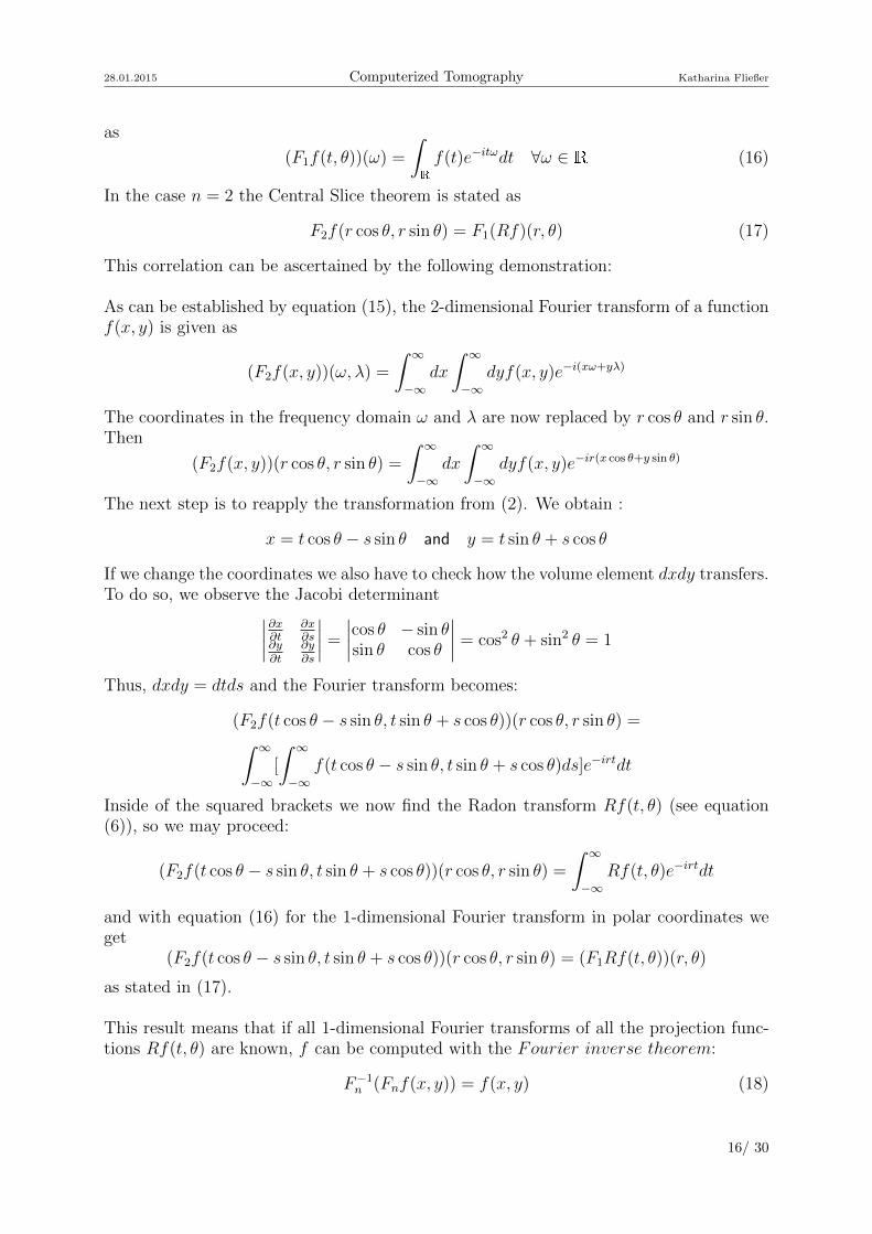
where i is the imaginary unit and xω is the standard inner product in n.The Radon transform in section 3 has been acting on a function f(t, θ) in polar co-ordinates, thus we are also interested in the Fourier transform for a function in polarcoordinates.The 1−dimensional Fourier transform for a function f(t, θ) in polar coordinates is given

15/ 30


as

(F1f(t, θ))(ω) =

�f(t)e−itω

dt ∀ω ∈ (16)

In the case n = 2 the Central Slice theorem is stated as

F2f(r cos θ, r sin θ) = F1(Rf)(r, θ) (17)

This correlation can be ascertained by the following demonstration:

As can be established by equation (15), the 2-dimensional Fourier transform of a functionf(x, y) is given as

(F2f(x, y))(ω,λ) =

� ∞

−∞dx

� ∞

−∞dyf(x, y)e−i(xω+yλ)

The coordinates in the frequency domain ω and λ are now replaced by r cos θ and r sin θ.Then

(F2f(x, y))(r cos θ, r sin θ) =

� ∞

−∞dx

� ∞

−∞dyf(x, y)e−ir(x cos θ+y sin θ)

The next step is to reapply the transformation from (2). We obtain :

x = t cos θ − s sin θ and y = t sin θ + s cos θ

If we change the coordinates we also have to check how the volume element dxdy transfers.To do so, we observe the Jacobi determinant

��∂x∂t

∂x∂s

∂y∂t

∂y∂s

�� =��cos θ − sin θsin θ cos θ

�� = cos2 θ + sin2θ = 1

Thus, dxdy = dtds and the Fourier transform becomes:

(F2f(t cos θ − s sin θ, t sin θ + s cos θ))(r cos θ, r sin θ) =� ∞

−∞[

� ∞

−∞f(t cos θ − s sin θ, t sin θ + s cos θ)ds]e−irt

dt

Inside of the squared brackets we now find the Radon transform Rf(t, θ) (see equation(6)), so we may proceed:

(F2f(t cos θ − s sin θ, t sin θ + s cos θ))(r cos θ, r sin θ) =

� ∞

−∞Rf(t, θ)e−irt

dt

and with equation (16) for the 1-dimensional Fourier transform in polar coordinates weget

(F2f(t cos θ − s sin θ, t sin θ + s cos θ))(r cos θ, r sin θ) = (F1Rf(t, θ))(r, θ)

as stated in (17).

This result means that if all 1-dimensional Fourier transforms of all the projection func-tions Rf(t, θ) are known, f can be computed with the Fourier inverse theorem:

F−1n (Fnf(x, y)) = f(x, y) (18)

16/ 30


and the inverse 2-dimensional Fourier Transform

F−12 f(ω,λ) =

� ∞

−∞

� ∞

−∞f(ω,λ)ei(xω+yλ)

dωdλ (19)

The problem with this reconstruction method, again, is the high computing power ittakes. At first the computer would have to calculate the 1-dimensional Fourier transformof all the measured projection functions pθ(t) to get (F1pθ(t))(r). Practically this is theFourier transform of the projection function Rf in the θ direction, for all θ. To obtain(F1pθ(t, θ))(r, θ) it would need to place all (F1pθ(t))(r) on a polar grid and afterwardsre−sample them into Cartesian space so that it is in the coordinate space of F2f(ω,λ)(see Figure 10). In the end the 2-dimensional inverse Fourier transform has to be calcu-

Figure 10: polar grid of (F1pθ(t, θ))(r, θ) and rectangular grid of F2f(ω,λ)

lated to yield f(x, y).

Particularly the re−sampling from polar to rectangular coordinates is a problem, be-cause it takes considerable spatial interpolation. This interpolation causes such a lot ofnoise that the resulting image is of no use for clinical application.

4.4 Filtered back projection

As stated above back projection leads to a smoothed version of the original image that wewant to reconstruct. The effects leading to the smoothing of the image can be correctedby the filtered back projection.The filtered back projection formula is the basis for image reconstruction and the methodused in clinical practise nowadays.The basic of filtered back projection is the following formula:

f(x, y) =1

2B{F−1[|r|F (Rf(r, θ))]}(x, y) (20)

where F and F−1 are the Fourier transform and the inverse Fourier transform, B is the

back projection and Rf(r, θ) is the Radon transform of f(r, θ).

At first we will examine how formula (20) is obtained:

17/ 30


We start with the Fourier inverse theorem

f(x, y) = F−12 F2f(x, y)

Written-out we have

f(x, y) =1

4π2

� ∞

−∞

� ∞

−∞F2f(X, Y )ei(xX+yY )

dXdY

Again we want to switch from Cartesian to polar coordinates, but this time we switchfrom X −→ r cos θ and Y −→ r sin θ with r ∈ and θ ∈ [0, π]. The Jacobi determinantnow gives

J =

��∂X∂r

∂Y∂r

∂X∂θ

∂Y∂θ

�� =��cos θ sin θ

−r sin θ r cos θ

�� = r cos2 θ + r sin2θ = r(cos2 θ + sin2

θ) = r

where r means |r|. Therefore the volume element reads dXdY = |r|drdθ. So we now have

f(x, y) =1

4π2

� π

0

� ∞

−∞F2f(r cos θ, r sin θ)e

ir(x cos θ+y sin θ)|r|drdθ

Using the Central Slice theorem (17) we obtain

f(x, y) =1

4π2

� π

0

� ∞

−∞F (Rf)(r, θ)eir(x cos θ+y sin θ)|r|drdθ (21)

For the next step we first make a little auxiliary calculation: The inverse Fourier transformof a function g(r), (F−1

g(r))(ω), for ω = x cos θ + y sin θ is

(F−1g(r))(x cos θ + y sin θ) =

1

2π

� ∞

−∞g(r)eir(x cos θ+y sin θ)

dr

If g happens to depend on a second variable θ but the Fourier transform is still 1-dimensional in r the inverse Fourier transform of g(r, θ) is

(F−1g(r, θ))(x cos θ + y sin θ, θ) =

1

2π

� ∞

−∞g(r, θ)eir(x cos θ+y sin θ)

dr

Now looking at (21) we see that the inner integral is nothing else than2πF−1[|r|F (Rf)(r, θ)](x cos θ + y sin θ, θ), and we obtain

f(x, y) =1

2π

� π

0

F−1[|r|F (Rf)(r, θ)](x cos θ + y sin θ, θ)dθ

Now we remember equation (11) for the back projection:

Bh(x, y) =1

π

� π

0

h(xcosθ + ysinθ)dθ

and finally arrive at our previously given expression

f(x, y) =1

2B{F−1[|r|F (Rf(r, θ))]}(x, y)

18/ 30


The |r| in the filtered back projection formula is very important. Without this factorthe inverse Fourier transform and the Fourier transform would just cancel out and leavethe back projection formula of f , of which we already know that it will not allow torecover the original function f(x, y), but rather its smoothed version.The filtered back projection formula assumes that the value of Rf(t, θ) is known for allpossible values (t, θ) to fully recover f(x, y), that would be an infinite number of values,but in practice there is only a finite number of angles at which X-ray samples can be sendthrough a tissue. From the resulting data an image has to be approximated.

If there was a function φ(t) such that (Fφ(t))(r) = |r|, the filtered back projection for-mula could be simplified. |r|F (Rf)(r, θ) would become [FφF (Rf)](r, θ) and since thepoint−wise product of two Fourier transforms is the Fourier transform of a convolution

(Fh)(Fg) = F (h ∗ g) (22)

were the convolution (h ∗ g) of f and g is defined as

(h ∗ g)(t) =� ∞

−∞h(τ)g(t− τ)dτ =

� ∞

−∞h(t− τ)g(τ)dτ (23)

we could write

F−1[|r|F (Rf)(r, θ)] = F

−1[F (φ ∗Rf)(r, θ)] = (φ ∗Rf)

and equation (20) for the filtered back projection would become:

f(x, y) =1

2B(φ ∗Rf)(x, y) (24)

This consideration will be very useful if we work with real data from a real X-ray ma-chine, because real data Rf will be affected by noise and we will use a function φ as aband−limited function.But first we will have a closer look upon the noise involved in Computerized Tomography.

4.4.1 Noise in Computerized Thomography

In Computerized Tomography ”noise” means visual disturbing signals which overlay theuseful signal without any futher information about the image.The main sources of noise in CT are

Quantum noise which arises from the fluctuations inherent in the detection of a finitenumber of X-ray quanta,

electronic noise caused by electric devices and

quantization noise from converting analog to digital signals.

If the useful signal becomes smaller the disturbing noise grows. Therefore the noisebecomes stronger if

the X-ray dose is small

the slice thickness is small, or

the diameter of the tissue, respectively of the patient, is large.

19/ 30


All of those conditions lead to a smaller number of X-ray quanta reaching the detectorand the detectors signal gets attenuated.

Usually noise has a high frequency, which is utilized by the filtered back projection.

4.4.2 Filtering

To obtain a formula which is less sensitive to noise, instead of the |r| in formula (20) wewill use another function of the frequency r, a low−pass filter.For signals were r is close to zero the low−pass filter function will nearly be |r|, but forlarge values of r it will vanish. The low−pass filter will be of the form A = Fφ, were φ isband−limited, so that we can use equation (24).We obtain:

f(x, y) ≈ 1

2B(F−1

A ∗Rf)(x, y) (25)

The function A(r) usually has the form

A(r) = |r|G(r)χ[−L,L](r)

where G(r) is a even function of r and G(0) = 1 in order to have an approximation of thefunction |r| near the origin and make sure that φ is real valued. χ[−L,L] is the characteristicfunction of the interval [−L,L] ∈ for L > 0. The characteristic function of a subsetT ⊆ X is the function for wich x ∈ X equals 1 if x ∈ T and 0 otherwise:

χT : X −→ {0, 1}

x �→�1 for x ∈ T

0 otherwise

In other words A(r) is only not vanishing on the interval [−L,L].Typical low−pass filters used in medical imaging are

• The Ram− Lak filter: A(r) = |r|χ[−L,L](r)

Figure 11: Ram−Lak filter for L = 10

• The Shepp− Logan filter: A(r) = |r|( sinπr2L

πr2L

)χ[−L,L](r) =

�2Lπ | sin( πr2L)| if |r| ≤ L

0 otherwise

20/ 30


Figure 12: Shepp−Logan filter for L = 10

• The low − pass cosine filter: A(r) = |r| cos( πr2L)χ[−L,L]

Figure 13: Cosine−Filter for L = 10

There are also many other filters like Butterworth, Hanning, Metz.The filter of choice for a given image reconstruction task is mainly a compromise betweenthe reduction of noise and the detail or contrast of the reproduced image. Also the imagesspatial frequency pattern of interest is of concern. The different filters do have differentcut−off frequencies.The Ram−Lak filter, shown in Figure 11 is a high−pass filter that blocks out low fre-quencies which cause blurring, like in back projection. If there are areas in an imagewhere the signal changes rapidly a high−pass filter sharpens the edges and gives bettercontrast. Disadvantage of Ram−Lak and other high−pass filters is that they let pass highfrequencies and as a consequence also noise. Therefore they are always combined with alow−pass filter.Low pass, or Smoothing filters, are Butterworth, Hanning, Metz, Shepp−Logan or thelow−pass cosine filter for exampel. These filters are defined by their cut−off frequency fc.No frequencies higher than their specific cut−off frequency can pass them. The highestcut−off frequency possible for any low−pass filter is the Nyquist frequency Nq. This isobvious, because Nq is the highest frequency that can be displayed in an image. Typi-cally the cut−off frequency is expressed as a fraction of the Nyquist frequency and variestypically from 0.2 to 1.0 times Nq (see reference [6]). The value of the cut−off frequencyeffects the image noise and resolution as well. If fc is high the spatial resolution is im-proved. Therefore much more detail can be seen in the image than with a lower cut−offfrequency but the image also remains noisy. A low cut−off frequency will cut off the noisebut decrease the images contrast by increasing the smoothing effect. The Shepp−Loganfilter produces the least smoothing and has the highest resolution.In Figure 15 different Filters are compared for the very noisy image Figure 14. On purpose

21/ 30


to compare their interference by noise each filter is investigated at three different cut−offfrequencies fc = 0, 2Nq,fc = 0, 5Nq and fc = 0, 95Nq. If the cut−off frequency is higherthe amount of noise grows.

Figure 14: Original noisy image, generated with the Mathematica-code for the Radon transform.

22/ 30


Figure 15: Comparison of different filters for reproducing the original image of Figure 14 each for threedifferent cutt−off frequencies: fc = 0, 2Nq,fc = 0, 5Nq and fc = 0, 95Nq. In the first row: the imagereconstructed without any filter. Unsurprisingly it does not depend on the frequency because it is notband−limited. In the second row: the Ram−Lak high−pass filter. The contrast is much better thanwithout the filter but the image is easily affected by noise. In the third row: the Shepp−Logan filter.The image appears very smooth, but the noise is cut off. In the last row is a combination of the low−passcosine and the Ram−Lak filter. As can be seen the image has sharp edges and is also not that muchbothered by noise. Images generated with Mathematica. 23/ 30


5 Discrete Problem

In the last sections we have set up a theory for image reconstruction, which is capableof reconstructing the image of a sample by knowing the intensity of X-rays sent throughthe sample along each line l(x cos θ+ y sin θ). We also considered noise reduction and thecomputational power needed. But what we have neglected so far is the impossibility ofsending an X-ray through each possible l(x cos θ + y sin θ). After all we are merely ableto send and detect a finite number of X-ray beams the way shown in section 2, Figure 3.As a consequence for clinical application the problem has to be discretised.In this section we will finally consider the approximations made for the discrete Problemand discuss the number of X-rays that is needed so we still get significant results.At first we address sampling which is the process of computing the values of a function,or a signal on a discrete set of points.

5.1 Sampling

If {xk}k∈ is a discrete number of points in than xk can be written as xk = kd forsome positive number d, called the sampling spacing. The sampling spacing d gives thesmallest details of f which can be perceived after sampling. The larger the value of d thebetter the resulting resolution and the more details can be seen. On the other hand, ifthe value of d is too large the amount of data is too big and the algorithm becomes veryslow. Therefore we need to find a optimal d which leads to detailed results but also allowsyou fast enough computation.

If we consider our signal as a sum of sinusoidal waves the smallest details perceivableare those of the same value as the smallest wavelength included. Since λ ∼ 1

ω the small-est details perceptible are also proportional to the maximum frequency ωmax. f is bandlimited, therefore Ff(ω) �= 0 only for ω ∈ [−L,L].One way to represent a wave−like function as the sum of simple sine waves is thecomplex Fourier series (Ff(x))(ω) =

�∞−∞ cne

2πnxω with the Fourier coefficient cn =

1ω

�∞−∞ f(x)e−i 2πnx

ω dx.For Ff periodically out of [−L,L] the Fourier coefficient becomes

cn =1

2L

� L

−L

f(x)e−iπnxL dx n ∈ .

If we compute, using the inverse Fourier theorem

2πf(nπ

L) = 2πF−1

Ff(nπ

L) =

�Ff(ω)eiωn

πLdω =

� L

−L

Ff(ω)eiωnπLdω =

=

� L

−L

f(x)eiωnπLdω = 2Lc−n

we obtainc−n =

π

Lf(n

π

L)

Ff(ω) is continuous, so the Fourier series becomes

Ff(ω) =∞�

n=−∞c−ne

−iωn πL =

π

L

∞�

n=−∞f(n

π

L)e−iωn π

L

24/ 30


One has f(x) = F−1(Ff(ω))(x). Therefore we compute:

F−1(Ff(ω))(x) =

∞�

−∞

1

2π

� ∞

−∞

π

Lf(n

π

L)e−iωn π

L eiωx

dω =∞�

−∞

1

2π

π

Lf(n

π

L)

� L

−L

eiω(x−n π

L )dω =

=∞�

−∞

1

2π

π

L

f(n πL)

i(x− nπL)

(eiω(x−n πL ))|L−L =

∞�

−∞f(n

π

L)ei(Lx−nπ) − e

−i(Lx−nπ)

2i(Lx− nπ)=

∞�

−∞f(n

π

L)sin(Lx− nπ)

Lx− nπ

What we obtain is

f(x) =∞�

−∞f(n

π

L)sin(Lx− nπ)

Lx− nπ(26)

which is called the Nyquist Theorem.The Nyquist Theorem means that the function f(x) can be fully reconstructed by f(n π

L)with n ∈ . Thereafter the sampling spacing d has to be d = π

L .The minimum wavelength can easily be figured out by looking at the maximum frequency.Since the maximum |ω| is L in Ff , the minimum wavelength is given by λmin = 2π

L ordepending on the sampling spacing λmin = 2d. This means that the optimal samplingspacing d is equal to half the size of the smallest detail present in the signal, which wouldbe λmin.

The number of angles at which X-ray beams are send through a sample is now givenby L

d . The more X-ray beams, respectively the more projection angels, the better the im-age. Figure 16 shows the evolving of a reconstruction with a growing number of projectionangles.

5.2 Discrete Functions and Filters

For the discrete filtered back projection formula we need to discretise each individualcomponent of the filtered back projection formula (25).

For a start we will look upon the descrete convolution. For two discrete functions f

and g and a finite set of values {fk = f(dk) : k = 0, ..., N − 1} the discrete convolution isgiven by

(f ∗ g)m =N−1�

j=0

fjgm−j ∀m ∈ (27)

The discrete convolution satisfies all principal properties of the standard convolution.

For the discrete Radon transform we recall what has been illustrated in the sections 2and 3. In Computerized Tomography the X-ray machine rotates by a fixed angle θ andat each angle the beams form a set of parallel lines (see Figure 3).The Radon transform is sampled for a finite number of angles θ ∈ [0, π) and, for eachangle, for a finite number of values of t.If N is the number of angles at which the machine takes scans, than the values of θ thatoccur are {k π

N , k = 1, ..., N − 1}.At each angle the set of parallel beams is composed of 2M + 1 equally spaced lines. d

is the distance between those lines. The object to be scanned should be centered at the

25/ 30


Figure 16: Recunstructed image with growing number of projection angels starting by a single X-raybeam in the first image and ending with 111 projection angels in the last. These images have been madewith the Radon Transformation code for Mathematica.

origin. Therefore the corresponding values of t are {jd : j = −M, ...,M}.The discrete Radon transform RDf is than defined as:

RDfj,k = Rf(jd, kπ

N) for j = −M, ...,M and k = 0, ...N − 1 (28)

What we also need is the discrete Fourier transform FDf and the descrete inverse Fourier transformF

−1D f . They are given by:

(FDf)j =N−1�

k=0

fke−2iπk j

N for j = 0, ..., N − 1 (29)

26/ 30


and

(F−1D f)j =

1

N

N−1�

k=0

fke2iπk j

N for j = 0, ..., N − 1 (30)

The properties of the Fourier transform and the inverse Fourier transform are still validfor discrete versions.

Other important components are the discrete filters for the discrete filtered back pro-jection and their inverse Fourier transforms. Here we will reconsider the filters used insection 4.4.2.

• The Ram − Lak filter has been given as A(r) = |r|χ[−L,L](r). Its inverse Fouriertransform is

F−1A(x) =

1

π[Lx sin(Lx)

x2−

2 sin2(Lx2 )

x2]

According to the Nyquist theorem F−1A(x) can be reconstructed from its values

taken at distances πL . This means we can just set x = n

πL and receive

F−1A(n

π

L) =

L2

2π[2 sin(nπ)

nπ− (

sin(nπ2 )nπ2

)2] (31)

• For the Shepp− Logan filter A(x) has been given as

A(r) = |r|( sinπr2L

πr2L

)χ[−L,L](r) =

�2Lπ | sin( πr2L)| if |r| ≤ L

0 otherwise. The inverse Fourier trans-

form for this function is

F−1A(x) =

L

π2[(cos(Lx− π

2 )

x− π2

−cos(Lx+ π

2 )

x+ π2

)− (1

x− π2L

− 1

x+ π2L

)].

Again we set x = nπL and obtain for n ∈

F−1A(n

π

L) =

4L2

π3(1− 4n2)(32)

• Finally we consider the low − pass cosine filter A(r) = |r| cos( πr2L)χ[−L,L].For this filter the inverse Fourier transform at integral multiples of the Nyquistdistance π

L is given by

F−1A(n

π

L) =

2L2

π2[π cos(πn)

1− 4n2− 2(1 + 4n2)

(1− 4n2)2] (33)

The only thing we still lack of for a discrete filtered back projection formula is adiscrete back projection.In the continuous case the back projection formula has been Bh(x, y) = 1

π

� π

0 h(xcosθ +ysinθ)dθ for values of the angle θ. As we figured out for the discrete Radon transform in

27/ 30


the discrete case the values of θ that occur are {k πN , k = 1, ..., N − 1}. For a function h

our discrete back projection BDh is therefore given as

BDh(x, y) =1

N

N−1�

k=0

h[x cos(kπ

N) + y sin(k

π

N), k

π

N] (34)

So now we do have all components and are able to compile our discrete filtered backprojection formula. We deduce from equation (25), that in the discrete case

f(x, y) ≈ 1

2BD[(F

−1D A) ∗ (RDf)](x, y) (35)

Figure 17 shows the crescent-shaped phantom and its reconstruction with the discretefiltered back projection using the Shepp-Logan Filter.

Figure 17: Crescent-shaped phantom and its reconstruction with the discrete filtered back projection,taken from Amos Sironi, Medical image reconstruction using kernel based methods (Universit‘a degli Studidi Padova, 2011)

28/ 30


6 Conclusions

In this thesis I discussed the physical and mathematic background of Computerized To-mography (CT) scanning and studied the problem of clinical image reconstruction.I took a closer look on what is done during CT scanning and what kind of information is ob-tained during the measurement. Next I inspected the mathematical aspect of CT scanningand discussed the Radon transform, which describes how we get an intensity−distributionout of an object with regions of different attenuation coefficients.I showed ways to re−transform this intensity−distribution so we might get the imageof the original object. First I introduced an algebraic method, which we figured out,takes too much computational power to be of use in practice. Then I demonstrated somemethods based on back projection of the Radon transform until we found that the bestopportunity is the filtered back projection method which is also the common method inclinical practice.At last I showed how this method is modified for computational application.

Even though the current procedure offers excellent results, medical image reconstruc-tion is still an active field of research. It will be interesting to see what progress can bemade in the coming years.

29/ 30


References

[1] Amos Sironi, ”Medical image reconstruction using kernal based methods.” Mas-ter’s thesis Universit‘a degli Studi di Padova, 2011

[2] Edwin L. Dove, Notes on Computerized Tomography, Script 51:060 BioimagingFundamentals, University of Iowa, College of Engineering, 2001

[3] Philippe P. Bruyant, J Nucl Med ,vol. 43 ,no. 10 1343-1358 (2002)

[4] A. Grillenberger und E. Fritsch, Computertomographie:Einfuhrung in ein mod-ernes bildgebendes Verfahren (Facultus Verlags− und Buchhandlungs AG, Berggasse5, 1090 Wien, 2007)

[5] T. H. Newton and D. G. Potts, Radiology of the Skull and Brain, Vol. 5: TechnicalAspects of Computed Tomography, (C. V. Mosby, St. Louis, 1981)

[6] M. Lyra and A. Ploussi, International Journal of Biomedical Imaging, Vol 2011,14, (2011)

[7] R. Kramme, Medizintechnik (Springer-Verlag, Heidelberg, 2011)

[8] J. Radon, ”Uber die Bestimmung von Funktionen durch ihre Integralwerte langsgewisser Mannigfaltigkeiten”, Ber. Verh. Sachs. Akad. Wiss. Leipzig – Math-Nat.kl., 69, 262–277, (1917).

30/ 30

computerized tomography - unigrazphysik.uni-graz.at/~uxh/diploma/fliesser15.pdf · computerized...

Documents