computer simulation studies of magnetic nanostructures

Faculty of Engineering, Science and Mathematics

School of Engineering Sciences

Computer simulation studies

of magnetic nanostructures

A thesis submitted in partial satisfaction

of the requirements for the degree of

Doctor of Philosophy

Richard P. Boardman

Computational Engineering and Design GroupSchool of Engineering Sciences

University of SouthamptonUnited Kingdom

Supervisors: Dr. Hans Fangohr, Prof. Simon J. Cox

17th May 2005

UNIVERSITY OF SOUTHAMPTON

ABSTRACT

FACULTY OF ENGINEERING, SCIENCE AND MATHEMATICS

SCHOOL OF ENGINEERING SCIENCES

Doctor of Philosophy

COMPUTER SIMULATION STUDIES OF MAGNETIC

NANOSTRUCTURES

Richard Paul Boardman

Scientific and economic interest has recently turned to smaller and smaller mag-

netic structures which can be used in hard disk drives, magnetoresistive random

access memory (MRAM), and other novel devices. For nanomagnets the geomet-

ric shape of the object becomes more important than other factors such as mag-

netocrystalline anisotropy — the smaller the object, the more strongly the shape

anisotropy affects the hysteresis loop.

We investigate the micromagnetic behaviour of ferromagnetic samples of var-

ious geometries using numerical methods. Finite differences and finite elements

are used to solve the Landau-Lifshitz-Gilbert and Brown’s equations in three di-

mensions. Simulations of basic geometric primitives such as cylinders and spheres

of sub-micron size orders provide hysteresis loops of the average magnetisation,

and additionally our computations allow the study of the microscopic configura-

tion of the magnetisation. We show different mechanisms of vortex penetration for

these geometries, and investigate part-spherical geometries whose magnetisation

pattern demonstrates qualities of other primitives.

Developing this further, we calculate the hysteresis loops for a droplet shape —

a part-sphere capped with an half-ellipsoid. This resembles the shapes formed by

some chemical self-assembly methods, a low-cost and efficient way of creating a

commercially viable product. When examining the magnetic microstructure of this

geometry we find different types of vortex behaviour, and reveal the dependence

of this on the physical characteristics of the droplet.

We also examine the hysteresis loops and magnetic structures of other geome-

tries formed through the self-assembly method such as antidots — honeycomb-like

arrays of spherical holes in a thin film. We show magnetisation patterns and com-

parison between experimental and computed magnetic force microscopy (MFM)

measurements.

ii

Contents

1 Introduction 1

1.1 Historical context . . . . . . . . . . . . . . . . . . . . . . . . . . . . . . 1

1.2 Modern magnetism . . . . . . . . . . . . . . . . . . . . . . . . . . . . . 3

1.3 Hard disk drives . . . . . . . . . . . . . . . . . . . . . . . . . . . . . . 4

1.4 Overview of relevant interactions . . . . . . . . . . . . . . . . . . . . . 5

1.5 Computer simulations . . . . . . . . . . . . . . . . . . . . . . . . . . . 6

1.6 Summary . . . . . . . . . . . . . . . . . . . . . . . . . . . . . . . . . . . 6

2 Micromagnetics 8

2.1 Introduction . . . . . . . . . . . . . . . . . . . . . . . . . . . . . . . . . 8

2.2 From quantum mechanics to micromagnetics . . . . . . . . . . . . . . 9

2.3 Interactions between atomic magnetic moments . . . . . . . . . . . . 10

2.3.1 Exchange energy . . . . . . . . . . . . . . . . . . . . . . . . . . 10

2.3.2 Anisotropy energy . . . . . . . . . . . . . . . . . . . . . . . . . 12

2.3.3 Zeeman energy . . . . . . . . . . . . . . . . . . . . . . . . . . . 14

2.3.4 Dipolar energy . . . . . . . . . . . . . . . . . . . . . . . . . . . 14

2.3.5 Total energy . . . . . . . . . . . . . . . . . . . . . . . . . . . . . 15

2.4 Micromagnetic description . . . . . . . . . . . . . . . . . . . . . . . . . 15

2.4.1 Exchange energy . . . . . . . . . . . . . . . . . . . . . . . . . . 16

2.4.2 Anisotropy energy . . . . . . . . . . . . . . . . . . . . . . . . . 17

2.4.3 Zeeman energy . . . . . . . . . . . . . . . . . . . . . . . . . . . 19

2.4.4 Dipolar energy . . . . . . . . . . . . . . . . . . . . . . . . . . . 19

2.5 From static to dynamic . . . . . . . . . . . . . . . . . . . . . . . . . . . 19

2.6 Computational models . . . . . . . . . . . . . . . . . . . . . . . . . . . 20

2.6.1 The Stoner-Wohlfarth model . . . . . . . . . . . . . . . . . . . 20

2.6.2 The Landau-Lifshitz-Gilbert equation . . . . . . . . . . . . . . 21

2.7 Simulation . . . . . . . . . . . . . . . . . . . . . . . . . . . . . . . . . . 22

2.7.1 Discretisation . . . . . . . . . . . . . . . . . . . . . . . . . . . . 22

2.7.2 LLG relaxation . . . . . . . . . . . . . . . . . . . . . . . . . . . 25

2.8 Micromagnetic systems . . . . . . . . . . . . . . . . . . . . . . . . . . . 26

2.8.1 The hysteresis loop . . . . . . . . . . . . . . . . . . . . . . . . . 26

2.8.2 Domains . . . . . . . . . . . . . . . . . . . . . . . . . . . . . . . 26

iii

2.8.3 States — microstructures of magnetisation . . . . . . . . . . . 28

2.9 Computational Issues . . . . . . . . . . . . . . . . . . . . . . . . . . . . 29

2.9.1 OOMMF software requirements . . . . . . . . . . . . . . . . . 30

2.9.2 magpar software requirements . . . . . . . . . . . . . . . . . . . 31

2.9.3 Post-processing . . . . . . . . . . . . . . . . . . . . . . . . . . . 33

2.9.4 Hardware requirements . . . . . . . . . . . . . . . . . . . . . . 33

2.9.5 Disk space . . . . . . . . . . . . . . . . . . . . . . . . . . . . . . 34

2.9.6 Commodity computing . . . . . . . . . . . . . . . . . . . . . . 35

2.9.7 Visualisation . . . . . . . . . . . . . . . . . . . . . . . . . . . . . 36

2.10 Applications . . . . . . . . . . . . . . . . . . . . . . . . . . . . . . . . . 39

2.10.1 Patterned and non-patterned media . . . . . . . . . . . . . . . 40

2.10.2 Magnetoresistive random access memory . . . . . . . . . . . . 41

3 Basic geometries: flat cylinders and spheres 42

3.1 Introduction . . . . . . . . . . . . . . . . . . . . . . . . . . . . . . . . . 42

3.2 Prior work . . . . . . . . . . . . . . . . . . . . . . . . . . . . . . . . . . 42

3.3 Parameterisation of geometry . . . . . . . . . . . . . . . . . . . . . . . 43

3.4 Flat cylinder . . . . . . . . . . . . . . . . . . . . . . . . . . . . . . . . . 45

3.5 Sphere . . . . . . . . . . . . . . . . . . . . . . . . . . . . . . . . . . . . 49

3.5.1 Finite differences and finite elements . . . . . . . . . . . . . . 49

3.5.2 Reversal mechanism . . . . . . . . . . . . . . . . . . . . . . . . 51

3.5.3 Size dependence . . . . . . . . . . . . . . . . . . . . . . . . . . 52

3.6 Summary . . . . . . . . . . . . . . . . . . . . . . . . . . . . . . . . . . . 56

4 Cones 57

4.1 Introduction . . . . . . . . . . . . . . . . . . . . . . . . . . . . . . . . . 57

4.2 Parameters . . . . . . . . . . . . . . . . . . . . . . . . . . . . . . . . . . 57

4.3 Results . . . . . . . . . . . . . . . . . . . . . . . . . . . . . . . . . . . . 58

4.4 Summary . . . . . . . . . . . . . . . . . . . . . . . . . . . . . . . . . . . 61

5 Nanodots 63

5.1 Introduction . . . . . . . . . . . . . . . . . . . . . . . . . . . . . . . . . 63

5.1.1 What is a nanodot? . . . . . . . . . . . . . . . . . . . . . . . . . 63

5.1.2 Lithography . . . . . . . . . . . . . . . . . . . . . . . . . . . . . 65

5.1.3 Self-assembly . . . . . . . . . . . . . . . . . . . . . . . . . . . . 65

5.2 Half-sphere . . . . . . . . . . . . . . . . . . . . . . . . . . . . . . . . . 66

5.2.1 Results . . . . . . . . . . . . . . . . . . . . . . . . . . . . . . . . 66

5.2.2 Discussion . . . . . . . . . . . . . . . . . . . . . . . . . . . . . . 67

5.3 Part-spherical nanodots . . . . . . . . . . . . . . . . . . . . . . . . . . 67

5.3.1 Parameters . . . . . . . . . . . . . . . . . . . . . . . . . . . . . . 69

5.3.2 Results . . . . . . . . . . . . . . . . . . . . . . . . . . . . . . . . 70

5.3.3 Comparing OOMMF and magpar . . . . . . . . . . . . . . . . . 72

iv

5.4 Multiple vortex states . . . . . . . . . . . . . . . . . . . . . . . . . . . . 73

5.5 “Droplet” nanodots . . . . . . . . . . . . . . . . . . . . . . . . . . . . . 75

5.5.1 Parameters . . . . . . . . . . . . . . . . . . . . . . . . . . . . . . 75

5.5.2 Reversal mechanism . . . . . . . . . . . . . . . . . . . . . . . . 77

5.5.3 Size dependence . . . . . . . . . . . . . . . . . . . . . . . . . . 80

5.6 Applying an out-of-plane external field . . . . . . . . . . . . . . . . . 80

5.7 Summary . . . . . . . . . . . . . . . . . . . . . . . . . . . . . . . . . . . 85

6 Antidots 86

6.1 Introduction . . . . . . . . . . . . . . . . . . . . . . . . . . . . . . . . . 86

6.1.1 The hexagonal lattice . . . . . . . . . . . . . . . . . . . . . . . . 87

6.2 Parameters of the antidot system . . . . . . . . . . . . . . . . . . . . . 89

6.3 Three-dimensional model . . . . . . . . . . . . . . . . . . . . . . . . . 90

6.4 Two-dimensional model . . . . . . . . . . . . . . . . . . . . . . . . . . 91

6.5 Stray field measurement . . . . . . . . . . . . . . . . . . . . . . . . . . 93

6.5.1 Numerical calculation of the stray field . . . . . . . . . . . . . 93

6.5.2 Stray field calculation through analytical techniques . . . . . . 94

6.6 Monte Carlo simulation . . . . . . . . . . . . . . . . . . . . . . . . . . 96

6.7 Results . . . . . . . . . . . . . . . . . . . . . . . . . . . . . . . . . . . . 98

6.8 Summary . . . . . . . . . . . . . . . . . . . . . . . . . . . . . . . . . . . 100

6.8.1 Outlook . . . . . . . . . . . . . . . . . . . . . . . . . . . . . . . 101

7 Summary and outlook 102

7.1 Summary . . . . . . . . . . . . . . . . . . . . . . . . . . . . . . . . . . . 102

A Analytical calculation of the stray field 104

B Supporting equations for the 3D/1D Monte Carlo method 111

C Material parameters 114

D CGS and SI (MKS) unit systems 116

E Complete simulation process 117

E.1 Notation . . . . . . . . . . . . . . . . . . . . . . . . . . . . . . . . . . . 117

F Constructive solid geometries 120

v

List of Tables

2.1 Magnetic moments of important transition metals (Kittel, 1996) . . . . 10

2.2 Exchange energy between parallel ferromagnetic moments . . . . . . 11

2.3 Properties of some common ferromagnetic materials . . . . . . . . . . 24

C.1 Properties of ferromagnetic materials . . . . . . . . . . . . . . . . . . . 115

D.1 The centimetre-gram-seconds (CGS) and the metre-kilogram-seconds

(SI) unit systems . . . . . . . . . . . . . . . . . . . . . . . . . . . . . . . 116

vi

List of Figures

1.1 William Gilbert’s magnetic model of the Earth . . . . . . . . . . . . . 2

1.2 Coulomb’s dipoles and Faraday’s lines of force . . . . . . . . . . . . . 3

1.3 An exploded view of the Hitachi Microdrive . . . . . . . . . . . . . . 5

2.1 Increasing storage density . . . . . . . . . . . . . . . . . . . . . . . . . 9

2.2 A three-platter IDE hard disk drive, manufactured by Fujitsu in 1999 10

2.3 Energy density due to uniaxial anisotropy . . . . . . . . . . . . . . . . 12

2.4 Cubic anisotropy energy surfaces . . . . . . . . . . . . . . . . . . . . . 13

2.5 The unit vectors of two moments Si and Sj . . . . . . . . . . . . . . . 16

2.6 The functions cosφ and 1− φ2

2 . . . . . . . . . . . . . . . . . . . . . . . 18

2.7 The effect of altering the number of cells in a geometry . . . . . . . . 23

2.8 Finite difference and finite element meshes . . . . . . . . . . . . . . . 24

2.9 Relaxed magnetisation from edge- and diagonally-aligned states . . 25

2.10 Typical hysteresis loops . . . . . . . . . . . . . . . . . . . . . . . . . . 27

2.11 Magnetic recording ideals . . . . . . . . . . . . . . . . . . . . . . . . . 27

2.12 A typical ferromagnet . . . . . . . . . . . . . . . . . . . . . . . . . . . 28

2.13 Domains formed in sample with closed flux . . . . . . . . . . . . . . . 28

2.14 Micromagnetic system states . . . . . . . . . . . . . . . . . . . . . . . 29

2.15 The simplified simulation process . . . . . . . . . . . . . . . . . . . . . 30

2.16 OOMMF memory requirements . . . . . . . . . . . . . . . . . . . . . . 31

2.17 Memory usage scaling with magpar . . . . . . . . . . . . . . . . . . . . 32

2.18 Memory usage of OOMMF and magpar . . . . . . . . . . . . . . . . . 32

2.19 A visualisation showing surface maps, streamlines, magnetisation

and an isosurface . . . . . . . . . . . . . . . . . . . . . . . . . . . . . . 37

2.20 Massless particles highlighting core vortex . . . . . . . . . . . . . . . 38

2.21 Out-of-plane and in-place vortices . . . . . . . . . . . . . . . . . . . . 39

2.22 Patterned and non-patterned media . . . . . . . . . . . . . . . . . . . 39

2.23 Magnetoresistive random access memory . . . . . . . . . . . . . . . . 41

3.1 Single-domain and vortex states . . . . . . . . . . . . . . . . . . . . . 43

3.2 Anisotropic simulation domain . . . . . . . . . . . . . . . . . . . . . . 44

3.3 Hysteresis loop for a flat nickel cylinder . . . . . . . . . . . . . . . . . 45

3.4 Cylinder overview with magnetisation in a high applied field . . . . 46

vii

3.5 Magnetisation in flat cylinder . . . . . . . . . . . . . . . . . . . . . . . 46

3.6 Flower state and onion state in a cylinder . . . . . . . . . . . . . . . . 47

3.7 Flat cylinder entering the vortex state . . . . . . . . . . . . . . . . . . 48

3.8 Flat cylinder just before leaving the vortex state . . . . . . . . . . . . 48

3.9 Height dependence of state transition in cylinders . . . . . . . . . . . 48

3.10 Phase diagram for nickel cylinders . . . . . . . . . . . . . . . . . . . . 49

3.11 Hysteresis loops for nickel spheres of diameter d=200nm . . . . . . . 50

3.12 Nickel sphere in high applied field showing spin tapering . . . . . . 52

3.13 Sphere at high applied field . . . . . . . . . . . . . . . . . . . . . . . . 53

3.14 Sphere immediately after entering the vortex state . . . . . . . . . . . 53

3.15 Sphere in vortex state . . . . . . . . . . . . . . . . . . . . . . . . . . . . 54

3.16 Sphere in late vortex state . . . . . . . . . . . . . . . . . . . . . . . . . 54

3.17 Size dependence of nickel spheres . . . . . . . . . . . . . . . . . . . . 55

3.18 Hysteresis loops for nickel spheres of diameter 50nm and 80nm . . . 55

4.1 Remanent magnetisation states in conical geometries . . . . . . . . . 58

4.2 Phase diagram of remanent states in cones . . . . . . . . . . . . . . . 59

4.3 Hysteresis loop for cone of d = h =100nm . . . . . . . . . . . . . . . . 60

4.4 Detailed points for cone reversal mechanism where d = h =100nm . 62

5.1 Scanning electron microscope image of a droplet array . . . . . . . . 64

5.2 MOKE measurements for a nickel dot array . . . . . . . . . . . . . . . 64

5.3 The double-template self-assembly technique . . . . . . . . . . . . . . 65

5.4 A typical nanodot “droplet” geometry . . . . . . . . . . . . . . . . . . 66

5.5 Hysteresis loop for a nickel half-sphere of diameter 200nm . . . . . . 67

5.6 Half-sphere at high applied field (point a in figure 5.5) . . . . . . . . 68

5.7 Half-sphere in remanent vortex state . . . . . . . . . . . . . . . . . . . 68

5.8 Half-sphere in late vortex state . . . . . . . . . . . . . . . . . . . . . . 69

5.9 Reversal mechanism phase diagram for part-spheres . . . . . . . . . 70

5.10 Reversal mechanism for d=50nm, h=0.5d . . . . . . . . . . . . . . . . . 71

5.11 Reversal mechanism for d=100nm, h=d . . . . . . . . . . . . . . . . . . 72

5.12 Hysteretic comparison of OOMMF (FD method) and magpar (hybrid

FE/BE method) . . . . . . . . . . . . . . . . . . . . . . . . . . . . . . . 73

5.13 Hysteresis loop for an isotropic nickel half-sphere of diameter 350nm 74

5.14 Two vortex states in an isotropic nickel half-sphere of diameter 350nm 75

5.15 Hysteresis loop for isotropic nickel half-sphere of diameter 750nm . . 76

5.16 Vortex “pinning” in three-quarter sphere . . . . . . . . . . . . . . . . 76

5.17 Reversal mechanism for nickel droplet of diameter 140nm . . . . . . 77

5.18 Hysteresis loops for droplets of bounding sphere diameter 140nm,

350nm and 500nm . . . . . . . . . . . . . . . . . . . . . . . . . . . . . . 78

5.19 Size dependence of coercive field in droplet nanodots . . . . . . . . . 79

viii

5.20 Comparison of experiment and simulation for nickel nanodots . . . . 80

5.21 Different hysteresis characteristics in droplet nanodots . . . . . . . . 81

5.22 Reversal mechanism of a droplet in a perpendicular applied field . . 82

5.23 Size dependence of out-of-plane coercive field in droplet nanodots . 83

5.24 Size dependence of out-of-plane and in-plane coercivity in droplet

nanodots . . . . . . . . . . . . . . . . . . . . . . . . . . . . . . . . . . . 84

6.1 The single-template self-assembly technique . . . . . . . . . . . . . . 87

6.2 Scanning electron microscope image of an antidot array . . . . . . . . 88

6.3 Oscillation of coercivity observed experimentally . . . . . . . . . . . . 88

6.4 Cubically and hexagonally packed spheres . . . . . . . . . . . . . . . 89

6.5 600x600x150nm cut of simple cubic nickel antispheres . . . . . . . . . 90

6.6 Magnetisation of a cobalt hexagonal antidot array in zero field . . . . 91

6.7 Hysteresis loop for permalloy antidot array . . . . . . . . . . . . . . . 92

6.8 Microscopic images of an antidot array . . . . . . . . . . . . . . . . . 94

6.9 Measured and computed demagnetising field of an antidot array in

zero field . . . . . . . . . . . . . . . . . . . . . . . . . . . . . . . . . . . 95

6.10 Measured and computed MFM signal of an antidot sample in a small

applied field . . . . . . . . . . . . . . . . . . . . . . . . . . . . . . . . . 96

6.11 Overview of Monte Carlo simulation . . . . . . . . . . . . . . . . . . . 97

6.12 Coercivity of small permalloy nanodots . . . . . . . . . . . . . . . . . 98

6.13 Coercivity of large permalloy nanodots . . . . . . . . . . . . . . . . . 99

6.14 Monte Carlo simulation results . . . . . . . . . . . . . . . . . . . . . . 100

6.15 MOKE and numerical measurements for cobalt antidots . . . . . . . 101

B.1 Polar plot of anisotropy energy and reversal conditions . . . . . . . . 112

E.1 The complete simulation process . . . . . . . . . . . . . . . . . . . . . 118

E.2 The OOMMF Oxs framework . . . . . . . . . . . . . . . . . . . . . . . 119

F.1 Simple constructive solid geometries . . . . . . . . . . . . . . . . . . . 121

ix

Declaration of Authorship

I, Richard Paul Boardman, declare that the thesis entitled Computer simulation stud-

ies of magnetic nanostructures and the work presented in it are my own. I confirm

that:

• this work was done wholly or mainly while in candidature for a research

degree at the University;

• where any part of this thesis has previously been submitted for a degree or

any other qualification at this University or any other institution, this has

been clearly stated;

• where I have consulted the published work of others, this is always clearly

attributed;

• where I have quoted from the work of others, the source is always given.

With the exception of such quotations, this thesis is entirely my own work;

• I have acknowledged all main sources of help;

• where the thesis is based on work done by myself jointly with others, I have

made clear exactly what was done by others and what I have contributed

myself;

• parts of this work have been published as:

– Micromagnetic simulation of ferromagnetic part-spherical particles Jour-

nal of Applied Physics, 95(11), pp. 7037-7039, June 2004 (with H. Fangohr,

A. V. Goncharov, A. A. Zhukov, P. A. J. de Groot and S. J. Cox)

– Micromagnetic simulation studies of ferromagnetic part-spheres Journal

of Applied Physics, accepted, to be published June 2005 (with J. Zimmer-

mann, H. Fangohr, A. A. Zhukov and P. A. J. de Groot)

– Oscillatory thickness dependence of the coercive field in 3D anti-dot ar-

rays from self-assembly Journal of Applied Physics, accepted, August 2004

(with A. A. Zhukov, A. V. Goncharov, P. A. J. de Groot, M. A. Ghanem, I.

S. El-Hallag, P. N. Bartlett, H. Fangohr, V. Novosad and G. Karapetrov)

– Oscillatory thickness dependence of the coercive field in magnetic 3D

anti-dot arrays Physical Review Letters, preprint at cond-mat/0406091, sub-

mitted June 2004 (with A. A. Zhukov, M. A. Ghanem, A. V. Goncharov, V.

Novosad, G. Karapetrov, H. Fangohr, P. N. Bartlett and P. A. J. de Groot)

x

Signed: ____________________________________________

Date: _____________________

xi

Acknowledgements

The author would like to acknowledge helpful discussions with Michael Donahue

of the Math, Statistics and Computational Science department within the National

Institute of Standards and Technology, to whom I am indebted for affording much

assistance with the finer points of the Object Oriented Micromagnetic Framework.

Many fruitful conversations with Werner Scholz of Seagate Technologies, Inc.

yielded further insight into the workings of magpar, for which I am most grateful.

I have had many indispensable meetings, e-mail and telephone conversations

with Alexander Zhukov, Alexander Goncharov and Peter de Groot of the School

of Physics and Astronomy at the University of Southampton, providing plots of

experimental data and guidance with theory — I am much obliged to you all.

My colleagues Jurgen Zimmermann and Giuliano Bordignon deserve many

thanks for their industrious verification of the equations and derivations found in

both the body of this thesis and the appendices.

My supervisor Hans Fangohr has provided thorough and dependable first-class

supervision and assistance where necessary and I am extraordinarily appreciative

of this.

I would like to thank my family for their tireless proof-reading of this work and

their devoted support, and to them I dedicate this thesis.

xii

Trademarks and copyright information

AMD, Opteron and Athlon are trademarks of Advanced Micro Devices

RenderMan R© and Pixar are registered trademarks of Pixar Animation Studios

The Visualization Toolkit (VTK) is copyright c© 1993-2002 Ken Martin, Will Schroeder,

Bill Lorensen

IBM is a trademark of International Business Machines

Intel, Pentium 4 and Xeon are trademarks of Intel Corp.

Philips is a registered trademark of Koninklijke Philips Electronics N.V.

Hitachi is a trademark of Hitachi Global Storage Technologies

Toshiba is a trademark of Toshiba Corporation.

Linux is a trademark of Linus Torvalds

The left-hand side of figure 1.3 is c© 2004 Griff Wason. http://www.griffwason.com

xiii

Chapter 1

Introduction

1.1 Historical context

Lodestone, rich in the mineral magnetite (Fe3O4), was known for its qualities of

attraction thousands of years ago. Historical accounts vary, but they indicate that

ancient Egyptian, Greek and Central American civilisations were familiar with it.

The Chinese first used a compass as a fortune-telling device and subsequently as a

directional indicator somewhere between 400 B.C. and 100 B.C., but surprisingly it

was not until later in the first millennium A.D. that a needle compass was used for

navigation.

In the thirteenth century Petri Pergrinus (Pierre de Maricourt) outlined the di-

rection to which the needle would point at various positions around a lodestone,

and from this ascertained that magnets had two regions, north and south.

The Elizabethan scientist William Gilbert demonstrated that the Earth was a gi-

ant magnet (Gilbert and Mottelay, 1600, 1991) and that this was responsible for the

directional alignment of a compass needle, additionally observing that the attrac-

tive effects of amber were, contrary to general belief at that juncture, not magnetic:

we now know this is a form of electrical attraction. Gilbert prepared and presented

Queen Elizabeth I of England with a magnetite model to demonstrate the mag-

netic behaviour of the Earth (figure 1.1) called a terrella, or “little earth”. When the

terrella was aligned with the poles of the Earth it would spin on its axis.

Gilbert is also responsible for providing the north-south polar analogy between

magnets and the Earth’s poles, and disposing of most of the magical legends sur-

rounding magnetism, though he did develop the somewhat esoteric notion that

the Earth had an anima, or “soul” which was the source of the magnetic field. The

anima was effective up to the orbis virtutis: the “orb of virtue”.

Gilbert can be credited with establishing magnetism as a scientific field. His

work fascinated Galileo Galilei who, influenced by Gilbert’s work (BBC, 2004), hy-

pothesised that the Earth orbited the Sun rather than the popular perception of the

time which was that the Sun (and everything else) revolved around the Earth.

1

��

��

anima

orbis virtutis

Figure 1.1: William Gilbert’s magnetic model of the Earth

In the mid-eighteenth century John Michell proposed that the attractive force

between two magnets can be calculated using the inverse square law, i.e. that if the

two entities are half as far apart, the force between them will be four times greater.

Charles Augustin de Coulomb verified this experimentally and indicated that if

one were to split a magnet then two new poles would be created (figure 1.2, left).

A professor at the University of Copenhagen, Hans Christian Oersted, observed

during a demonstration that the needle of a compass was deflected whenever he

turned on an electric current; this was the first recorded instance of the relationship

between magnetism and electricity. Andre Ampere, a French physicist, confirmed

this and just one week after the initial observation by Oersted had developed an

equation to calculate the magnetic force between electric currents.

Towards the end of the 1830s Michael Faraday propounded the concept of lines

of force, nowadays known as magnetic field lines, as a way of visualising the mag-

netic field of an object (figure 1.2, right); these can be seen when dusting iron filings

around a traditional bar magnet. Faraday was also responsible for creating the elec-

tric generator and motor.

During the 1850s and 1860s James Clerk Maxwell developed mathematical equa-

tions derived from mechanical models which described the electricity and mag-

netism, the relationship between them, and Faraday’s lines of force. These equa-

tions were published in 1873 and defined classical electromagnetism.

2

Figure 1.2: Coulomb’s theory (left) was that if one were to break a magnet into two parts then twonew poles would form at the broken ends. Magnetic field lines or “lines of force” (right)as demonstrated by Michael Faraday.

1.2 Modern magnetism

Augustin Jean Fresnel, best known for his work with light, mentioned in a letter to

Ampere that the electric currents responsible for magnetic forces might operate at

microscopic

lengths.

At the start of the twentieth century another French physicist, Pierre Weiss, de-

veloped his theory of magnetism, which began to describe magnetic interactions at

the microscopic scale. With the advent of quantum mechanics, magnetic interac-

tions became better understood.

Building on these new principles, magnetic recording systems developed at the

end of the nineteenth century were improved and the consequent development of

magnetic tape eventually paved the way for the audio tape recorder in the middle

of the twentieth century.

Today, magnets are pervasive in daily life:

• Cars contain magnets in starter motors, electric windows, door locking sys-

tems, electronic relays and alternators.

• Kitchens have magnetic motors in refrigerators, microwave ovens, washing

machines and tumble dryers.

• Entertainment systems such as video recorders, CD and DVD players, audio

tape recorders and minidisc players all contain motors. These motors contain

magnets.

• Televisions and monitors use magnets to deflect and position the electron

beam used to create an image, as well as high-voltage electromagnets to de-

gauss the tube. Degaussing eliminates apparent colouring problems with the

display tubes in these devices.

3

• Electric bells in telephones, alarms and doorbells contain magnetic ringers.

• Medical applications include the use of magnetic fluids in eye surgery and

drug delivery, as guides in keyhole surgery, prosthetics, cancer therapy and

magnetic resonance imaging.

Magnets can also be found on the reverse side of credit cards, in cooling fans,

power station generators and audio speakers. One of the fastest-developing areas

in magnetism is in the area of data storage in computers, particularly hard disk

drives.

1.3 Hard disk drives

Magnetic systems have been used in recent years for the long-term storage of data

in computers. The first hard disk came in 1956 from IBM inside their RAMAC

(Random Access Method of Accounting and Control) computer, capable of storing

100,000 characters on each of fifty 24-inch disk platters and constructed from iron

oxide and aluminium. These disks had a data, or areal, density of around 2 kilobits

per square inch.

Seventeen years later IBM released the Winchester hard disk, containing the

basic technologies used in modern hard disk drives: a very small read/write head

capable of “skiing” around 1/18,000,000 of an inch above the surface of the disk.

The Winchester had an areal density of 1.7 megabits per square inch.

Seagate Storage Technology developed the first hard disk for personal comput-

ers in 1980. Although this disk had a similar capacity to the RAMAC, the entire

assembly fit into a 5.25 inch enclosure (form factor): the same width and double

the height of a standard modern CD-ROM drive. Three years later, Rodime intro-

duced a hard disk in a 3.5 inch form factor, and in 1985 Quantum attached this to a

hard card which plugged directly into a personal computer’s system board.

This form factor evolution continued throughout the late 1980s, until standard

3.5 inch hard drives with integrated electronics appeared. Introduced by Conner in

1988, these had the same physical dimensions as a standard desktop PC hard disk

drive today. The same year saw the first 2.5 inch hard drive, now the de facto stan-

dard for laptop computers, though the 1.8 inch form factor is gaining popularity

with slimline and sub-notebook sized laptops.

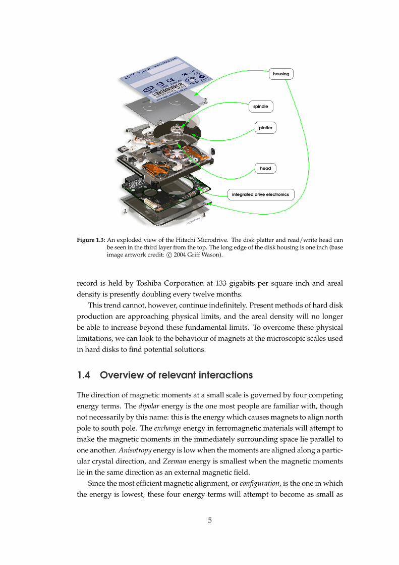
Currently the smallest hard disk drive with this configuration is the Hitachi

Microdrive (figure 1.3), having a one inch form factor and a height of just five mil-

limetres but with a capacity of four gigabytes.

Hard disk drive manufacturers are constantly looking for ways to improve areal

density, as this equates to a greater storage capacity. Areal density is widely re-

garded as the crucial metric driving the hard disk industry. The highest areal den-

sity today is more than fifty million times greater than in the late 1950s: the present

4

spindle

head

platter

housing

integrated drive electronics

Figure 1.3: An exploded view of the Hitachi Microdrive. The disk platter and read/write head canbe seen in the third layer from the top. The long edge of the disk housing is one inch (baseimage artwork credit: c© 2004 Griff Wason).

record is held by Toshiba Corporation at 133 gigabits per square inch and areal

density is presently doubling every twelve months.

This trend cannot, however, continue indefinitely. Present methods of hard disk

production are approaching physical limits, and the areal density will no longer

be able to increase beyond these fundamental limits. To overcome these physical

limitations, we can look to the behaviour of magnets at the microscopic scales used

in hard disks to find potential solutions.

1.4 Overview of relevant interactions

The direction of magnetic moments at a small scale is governed by four competing

energy terms. The dipolar energy is the one most people are familiar with, though

not necessarily by this name: this is the energy which causes magnets to align north

pole to south pole. The exchange energy in ferromagnetic materials will attempt to

make the magnetic moments in the immediately surrounding space lie parallel to

one another. Anisotropy energy is low when the moments are aligned along a partic-

ular crystal direction, and Zeeman energy is smallest when the magnetic moments

lie in the same direction as an external magnetic field.

Since the most efficient magnetic alignment, or configuration, is the one in which

the energy is lowest, these four energy terms will attempt to become as small as

5

possible at the expense of their peers: this results in very rich, complex and aes-

thetically attractive physics.

The competition of these interactions under different conditions is responsible

for the overall behaviour of a magnetic system, and the ability to compute this

yields a greater understanding of such systems.

1.5 Computer simulations

Analytical models exist for some magnetic systems, however for these models so-

lutions are only practical for simple cases. Experiments allow observations to be

made of real systems, but we are limited to the detail which can be extracted from

these measurements.

When computational resources are available, more complicated models can be

used which provide a link between experiment and theory. The motivation for us-

ing computer simulations is two-fold: firstly, it is possible to interpret experimental

results, and secondly new designs can be predicted and subsequently developed,

reducing costs.

1.6 Summary

Scientific and economic interest has recently turned to smaller and smaller mag-

netic structures which can be used in hard disk drives, magnetoresistive random

access memory (MRAM), and other novel devices. For nanomagnets — magnets

with a size order of 10−7 metres and below, more than five hundred times smaller

than the width of a human hair — the geometric shape of the object becomes more

important; the smaller the object, the more strongly the shape anisotropy affects the

hysteresis loop.

This thesis reports on investigations of these magnetic nanostructures.

Chapter 2 briefly summarises the origins of magnetism, the applications of mi-

cromagnetism in modern digital data storage — specifically hard disk media and

magnetoresistive random access memory — and some of the theories behind mi-

cromagnetics pertaining to our simulation work. Additionally, this chapter covers

the methods we use in more detail with respect to geometry and computation, and

also touches on post-simulation visualisation.

Chapter 3 investigates the properties of basic primitives. We study numerically

the magnetisation reversal of a flat cylinder and a sphere, and provide studies of

size dependence for these geometries.

Chapter 4 discusses the magnetic reversal behaviour of conical particles, and

presents a magnetisation remanence phase diagram as a function of diameter and

height.

6

Chapter 5 considers the simulation of “nanodots”. These tiny part-spherical ge-

ometries can be formed through a chemical self-assembly double template method,

and numerical studies assist with the interpretation of experimental data.

In Chapter 6, we study the magnetic behaviour of close-packed spherical holes,

or antispheres, produced through a self-assembly template method.

Finally in Chapter 7 we summarise our findings and provide an outlook for

future research.

7

Chapter 2

Micromagnetics

2.1 Introduction

After IBM attained an areal recording density of 1Gbit/in2 (Tsang et al., 1993, 1990)

— half a million times greater than RAMAC — the growth of areal density of a

consumer hard disk drive has been approaching 100% every twelve months. Fol-

lowing current trends the next decade should witness the advent of an areal density

of 1Tbit/in2 (Tarnopolsky, 2004, Wood, 2000, Wood et al., 2002).

Since modern hard disk drive technology is converging on fundamental limits

(see figures 2.1, 2.2) new approaches must be considered. Micromagnetic simula-

tion is an important method of addressing these limits. Further discussion of the

applications of micromagnetic modelling can be seen in section 2.10.

In sections 2.2 to 2.6 we provide an overview of micromagnetics.

In section 2.3 we describe the different interactions and associated energies of a

system of magnetic moments µ.

Section 2.4 describes the micromagnetic approach when the discrete, atomistic

nature of matter is ignored and the magnetisation is represented as a continuous

function of space.

In sections 2.5 and 2.6 the Landau-Lifshitz Gilbert equations and the Stoner-

Wohlfarth model are introduced.

Sections 2.7 to 2.10 describe the simulation packages used in this work and as-

sociated hardware and software requirements.

Micromagnetism as a field — i.e. that which deals specifically with the be-

haviour of ferromagnetic materials at fine (1× 10−6 metre) length scales — was in-

troduced in 1963 when William Fuller Brown Jr. published his paper on antiparallel

domain wall structure (Brown, 1963); however until comparatively recently compu-

tational micromagnetics — particularly when three-dimensional problems are con-

sidered — has been prohibitively expensive in terms of computational power, but

now a modern desktop PC is capable of performing small micromagnetic simula-

tions within a few days.

8

1 10 100 1000Bit edge size (nm)

10-1

100

101

102

103

104

105

Sto

rage c

apacity (

Gbits/in

2)

1 G

10 G

100 G

1 T

10 T

100 T

1 P

Multip

latter

3.5

" hard

dis

k theore

tical sto

rage (

byte

s)

1989: First magnetoresistive head

allows 1Gbit per square inch

15.2 Gbit per square inch density

2000: IBM Microdrive achieves

2003: Seagate set areal density record

with 101 Gbits per square inch

2003: Hitachi announce 4Gb Microdrive

with a 60 Gbit per square inch density

Likely density limit for

non−patterned media

2002: Prototype patterned media from

IBM attains 74 Gbits per square inchProbable density limit for

patterned media (2Tb/sq in)

Width of ten Fe atoms

if placed side−by−side

Figure 2.1: As the area in which a bit can be stored decreases, the overall storage capacity increasesin O(1/n2) assuming a square bit of edge length n; the scale on the right indicates thecapacity of a four-platter double-sided 3.5” hard disk, ignoring spindle size and actuationoverheads.

2.2 From quantum mechanics to micromagnetics

To clarify some of the terminology, concepts and fundamental models which are

essential to computational micromagnetics, this section will briefly discuss some

of these. More detailed accounts can be found in Brown (1963), O’Handley (1999),

Aharoni (2000) and Blundell (2001).

The magnetic moment is derived from the angular momentum of electrons in

an atom. For free atoms, this is a combination of electron spin and orbital momen-

tum (O’Handley, 1999):

µ = −gµB(L+ S) (2.1)

where µ is the magnetic moment, g is the generalised Lande factor (≈2), µB is

the Bohr magneton (9.2741×10−24 A·m2), L is the orbital momentum and S is the

electron spin.

When materials are solids, the spin component S dominates the magnetic mo-

9

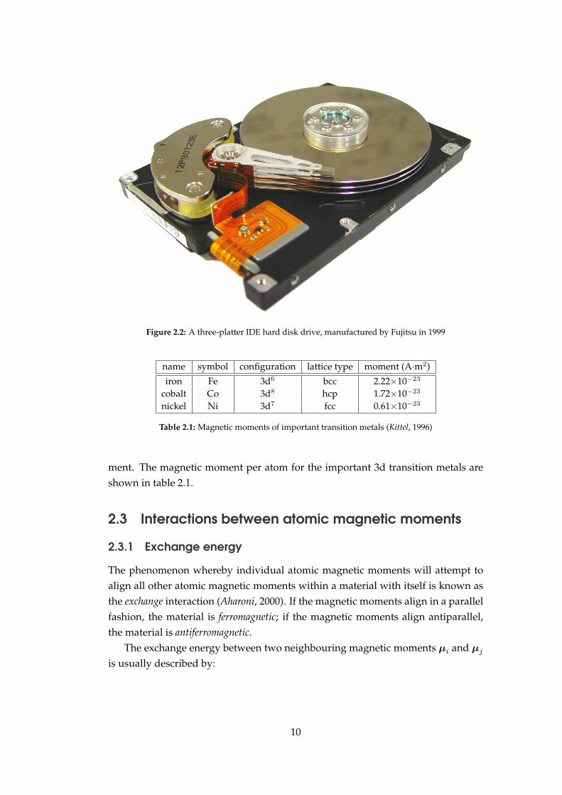
Figure 2.2: A three-platter IDE hard disk drive, manufactured by Fujitsu in 1999

name symbol configuration lattice type moment (A·m2)

iron Fe 3d6 bcc 2.22×10−23

cobalt Co 3d8 hcp 1.72×10−23

nickel Ni 3d7 fcc 0.61×10−23

Table 2.1: Magnetic moments of important transition metals (Kittel, 1996)

ment. The magnetic moment per atom for the important 3d transition metals are

shown in table 2.1.

2.3 Interactions between atomic magnetic moments

2.3.1 Exchange energy

The phenomenon whereby individual atomic magnetic moments will attempt to

align all other atomic magnetic moments within a material with itself is known as

the exchange interaction (Aharoni, 2000). If the magnetic moments align in a parallel

fashion, the material is ferromagnetic; if the magnetic moments align antiparallel,

the material is antiferromagnetic.

The exchange energy between two neighbouring magnetic moments µi and µj

is usually described by:

10

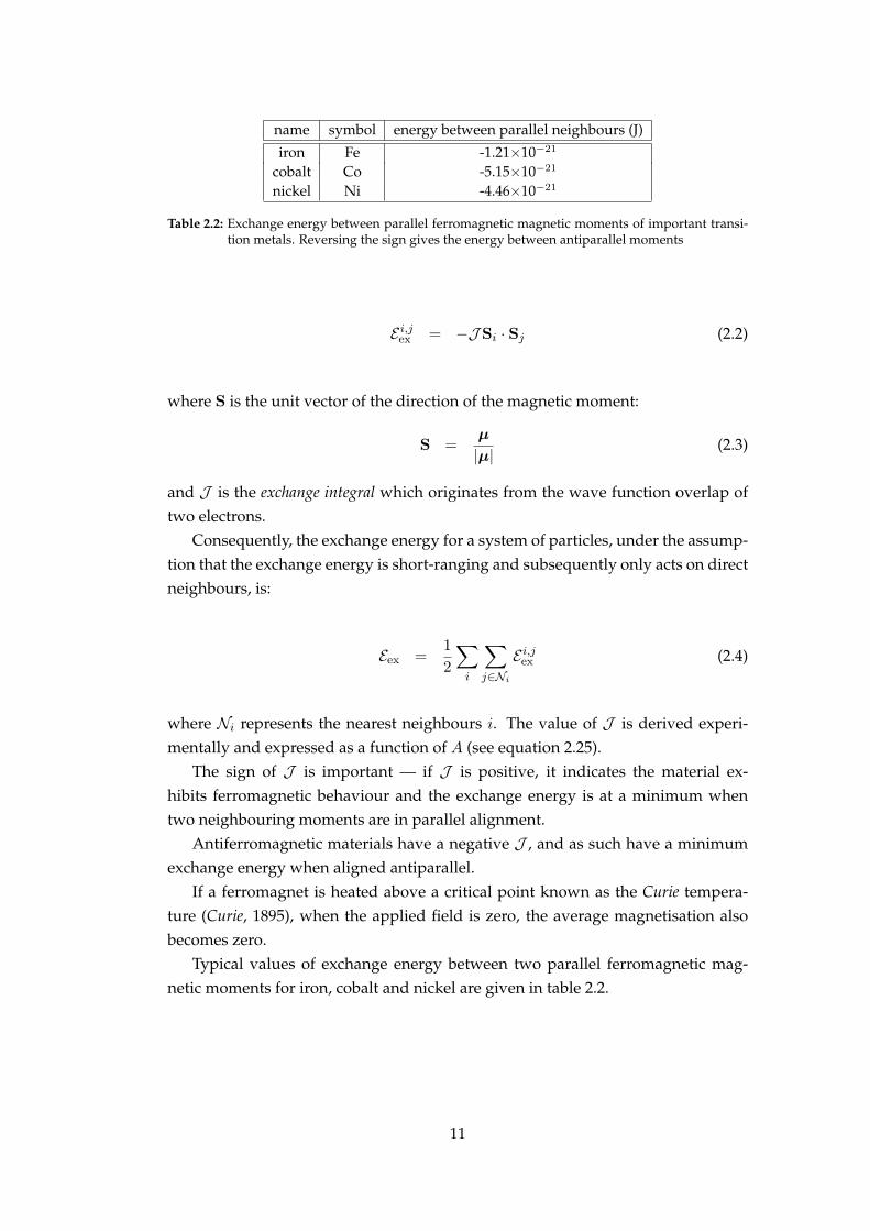
name symbol energy between parallel neighbours (J)

iron Fe -1.21×10−21

cobalt Co -5.15×10−21

nickel Ni -4.46×10−21

Table 2.2: Exchange energy between parallel ferromagnetic magnetic moments of important transi-tion metals. Reversing the sign gives the energy between antiparallel moments

E i,jex = −JSi · Sj (2.2)

where S is the unit vector of the direction of the magnetic moment:

S =µ

|µ| (2.3)

and J is the exchange integral which originates from the wave function overlap of

two electrons.

Consequently, the exchange energy for a system of particles, under the assump-

tion that the exchange energy is short-ranging and subsequently only acts on direct

neighbours, is:

Eex =1

2

∑

i

∑

j∈Ni

E i,jex (2.4)

where Ni represents the nearest neighbours i. The value of J is derived experi-

mentally and expressed as a function of A (see equation 2.25).

The sign of J is important — if J is positive, it indicates the material ex-

hibits ferromagnetic behaviour and the exchange energy is at a minimum when

two neighbouring moments are in parallel alignment.

Antiferromagnetic materials have a negative J , and as such have a minimum

exchange energy when aligned antiparallel.

If a ferromagnet is heated above a critical point known as the Curie tempera-

ture (Curie, 1895), when the applied field is zero, the average magnetisation also

becomes zero.

Typical values of exchange energy between two parallel ferromagnetic mag-

netic moments for iron, cobalt and nickel are given in table 2.2.

11

0 1 2 3 4 5 6angle from magnetic moment θ (radians)

-8×104

-6×104

-4×104

-2×104

0

an

iso

tro

py e

ne

rgy ω

u (

J/m

3)

Niα-Fe

Figure 2.3: Energy density due to uniaxial anisotropy as a function of the angle θ from a magneticmoment µ. The maximum energy has been normalised to zero for clarity.

2.3.2 Anisotropy energy

Anisotropy is a dependence of energy level on some direction. If the magnetic

moments in a material have a bias towards one particular direction (the easy axis)

then the material is said to have uniaxial anisotropy, like cobalt. If the bias is to-

wards many particular directions, then the material has multiple easy axes and it

possesses cubic anisotropy (see figure 2.4). Cubic crystals such as iron and nickel

have this property (Aharoni, 2000, p86). Uniaxial and cubic anisotropy are forms

of magnetocrystalline anisotropy as their properties in this respect arise from the

crystalline structure of the material.

The anisotropy energy in transition metal magnets arises from spin-orbit cou-

pling. The typical fourth-order approximation of the parameterisation of uniaxial

anisotropy (expressed as an energy density) is (Aharoni, 2000):

E iuni = −K1 cos

2(θi)−K2 cos4(θi) (2.5)

= K1S2z +K2S

4z (2.6)

where θi is the angle between Si and the easy axis (being here the component of S in

the direction of the crystallographic axis, z). K1 and K2 are temperature-dependent

12

yx

z

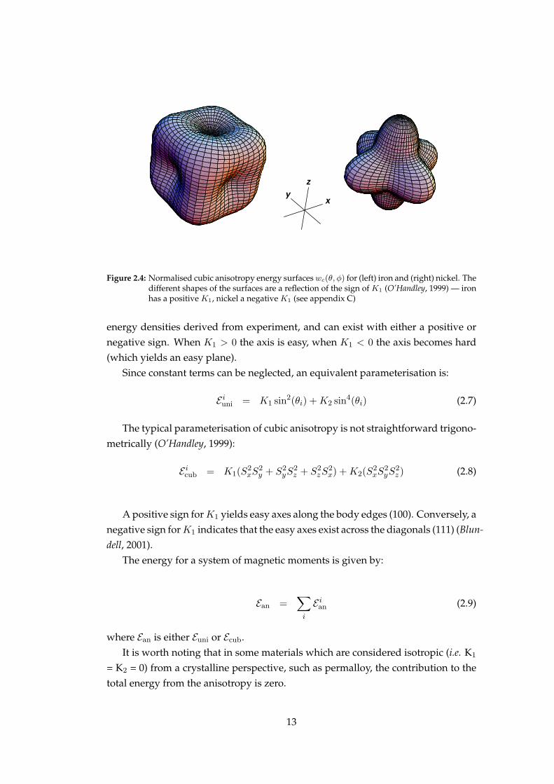
Figure 2.4: Normalised cubic anisotropy energy surfaces wc(θ, φ) for (left) iron and (right) nickel. Thedifferent shapes of the surfaces are a reflection of the sign of K1 (O’Handley, 1999) — ironhas a positive K1, nickel a negative K1 (see appendix C)

energy densities derived from experiment, and can exist with either a positive or

negative sign. When K1 > 0 the axis is easy, when K1 < 0 the axis becomes hard

(which yields an easy plane).

Since constant terms can be neglected, an equivalent parameterisation is:

E iuni = K1 sin

2(θi) +K2 sin4(θi) (2.7)

The typical parameterisation of cubic anisotropy is not straightforward trigono-

metrically (O’Handley, 1999):

E icub = K1(S

2xS

2y + S2

yS2z + S2

zS2x) +K2(S

2xS

2yS

2z ) (2.8)

A positive sign for K1 yields easy axes along the body edges (100). Conversely, a

negative sign for K1 indicates that the easy axes exist across the diagonals (111) (Blun-

dell, 2001).

The energy for a system of magnetic moments is given by:

Ean =∑

i

E ian (2.9)

where Ean is either Euni or Ecub.

It is worth noting that in some materials which are considered isotropic (i.e. K1

= K2 = 0) from a crystalline perspective, such as permalloy, the contribution to the

total energy from the anisotropy is zero.

13

There are other types of anisotropy than magnetocrystalline. Magnetostriction is

an anisotropy caused by the expansion or contraction of a ferromagnet along the

direction of the magnetisation (Aharoni, 2000, p87). The so-called shape anisotropy

(Paine et al., 1955) (also known as “configurational stability” (Ha et al., 2003)) is the

direction in which the magnetisation will prefer to lie on account of the physical

geometry of the sample. This becomes more and more influential the smaller one’s

sample becomes. This is one of the properties we investigate in this report.

2.3.3 Zeeman energy

The energy of a magnetic moment µ in an applied magnetic field H is:

E iZe = −µ0µi ·Hi (2.10)

For a system of atoms:

EZe =∑

i

E iZe (2.11)

The Zeeman energy is at a minimum when all the magnetic moments in a sam-

ple are in alignment with the applied field.

2.3.4 Dipolar energy

Dipolar energy (often called magnetostatic or demagnetising energy) is the resul-

tant energy from the interaction of magnetic moments with each other. Two mag-

netic moments at positions ri and rj have the dipolar energy:

E i,jdi = µ0

(

µi · µj

|rij |3− 3(µi · rij)(µj · rij)

|rij |5)

(2.12)

where

rij = rj − ri (2.13)

For N magnetic moments this becomes:

14

Edi =1

2

N∑

i=1

∑

j 6=i

E i,jdi (2.14)

Computing the dipolar energy is the most expensive part of any micromagnetic

simulation as the dipolar energy is a long-range interaction and therefore must

consider the interaction of each magnetic moment µi with every other magnetic

moment µj .

2.3.5 Total energy

Combining equations 2.4, 2.9, 2.11 and 2.14 yields the total energy:

E =1

2

∑

i

∑

j∈Ni

E i,jex +

∑

i

E ian +

∑

i

E iZe +

1

2

N∑

i

∑

j 6=i

E i,jdi (2.15)

The number of atoms in comparatively small systems is large. Assuming a

cubic structure and a lattice spacing of 2.5A as in iron, cobalt or nickel, a cube of

edge length 100nm would contain 6.4×107 atoms.

2.4 Micromagnetic description

Since numerical computations based on the equations in section 2.3 are at an atomic

level, they are historically limited to simple cases containing not too many degrees

of freedom (Aharoni, 2000, p173). For larger problems other techniques must be

used.

Brown (1963) suggested a theory which is referred to as micromagnetic theory.

Instead of considering individual magnetic moments, a continuous magnetisation

function M is used to approximate the atomic interaction described above. The

magnetisation represents the locally averaged density of magnetic moments:

M(r) =1

V (r,∆r)

∑

i∈J(r,∆r)

µi (2.16)

where V (r,∆r) is a sphere of radius ∆r placed at r and J(r,∆r) is the set of indices:

J = {i : ri ∈ V (r,∆r)} (2.17)

15

Sj

Si

Si

Sj

Sj − Si

φi,jri,j

Figure 2.5: The unit vectors of two moments Si and Sj

for magnetic moments µi that are located inside the volume V (r,∆r).

This averaging can be performed over the scale of the exchange length (see

equation 2.40) and will always contain many magnetic moments.

M(r) is assumed to be a continuous and differentiable function which allows

the expression of the interactions described above using differential operators. The

resulting equations can be solved analytically (if possible) or numerically.

2.4.1 Exchange energy

Taking the atomic representation for exchange energy between two moments (equa-

tion 2.2), we can assume that the angle between two neighbouring spins is φi,j . The

sum of all the exchange energies based on equation 2.4 can be rewritten as:

Eex = −J S2∑

i

∑

j∈Ni

cosφi,j (2.18)

where S = 1 since S is a unit vector (equation 2.3) and for small values of φi,j we

use the leading terms in the Taylor expansion of cosφi,j (figure 2.6):

cosφi,j ≈ 1−φ2i,j

2(2.19)

With this assumption, equation 2.18 can be rewritten:

Eex = K +J S2

2

∑

i

N∑

j 6=i

φ2i,j (2.20)

16

where K is a constant. Since Si =M(ri)Ms

and |Si| = |Sj | = 1 (figure 2.5):

|φi,j | ≈ |Si − Sj | (2.21)

= a|Si − Sj |

a(2.22)

and|Si−Sj |

a approximates the spatial derivative of S over the lattice spacing a.

If we take ri,j to be a lattice translation vector of magnitude a as in figure 2.5,

the directional derivative ∇ri,jS can be used to express |Si − Sj |.Inserting this into equation 2.18, the exchange energy can now be represented

as (Blundell, 2001):

Eex = −J S2∑

i

N∑

j 6=i

[(ri,j · ∇)S]2 (2.23)

= −J S2a2∑

i

N∑

j 6=i

[

(∇mx)2 + (∇my)

2 + (∇mz)2]

(2.24)

if we take ri,j outside the summations and redefine this as a (the nearest neighbour

distance). Since we will integrate over volume to obtain the continuous represen-

tation, if we consider a unit cell site number z = 1, 2 or 4 (for simple cubic, body-

centred cubic and face-centred cubic respectively), we can define the exchange cou-

pling constant (Aharoni, 2000):

A =J S2z

a(2.25)

We can now ignore the discrete lattice, yielding the continuous form:

Eex = A

∫

V

[

(∇Sx)2 + (∇Sy)

2 + (∇Sz)2]

d3r (2.26)

2.4.2 Anisotropy energy

The continuous form of the anisotropy energy is computed by integrating the

anisotropy energy wan (Aharoni, 2000), which is in the form of either equation 2.5

or 2.8:

Ean =

∫

Vwand

3r (2.27)

17

0 0.5 1 1.5 2φ (radians)

-1

-0.5

0

0.5

1

cos φ

1 - φ2/2

cos φ - (1 - φ2/2)

Figure 2.6: The functions cosφ (solid black) and 1− φ2

2(dashed red). The dotted green line represents

the difference between the two functions

18

2.4.3 Zeeman energy

By ignoring the discrete lattice, equation 2.11 becomes (Aharoni, 2000):

EZe = −µ0

∫

VM(r) ·H(r)d3r (2.28)

2.4.4 Dipolar energy

The dipolar energy can be represented continuously by:

Edi = −µ0

∫

VHde(r) ·M(r)d3r (2.29)

where Hde(r) is the demagnetising field with components contributed from the di-

vergence of magnetisation within the volume and surface poles (O’Handley, 1999):

Hde(r) =1

4π

(

−∫

Vd3r′∇ ·M(r′)

r− r′

|r− r′|3 +

∫

Sd2r′n ·M(r′)

r− r′

|r− r′|3)

(2.30)

and n is the surface normal.

A complete derivation of Hde is given in Brown (1963), Aharoni (2000) and Blun-

dell (2001).

2.5 From static to dynamic

In order to study dynamical phenomena we can combine the equations above with

the work of Landau, Lifshitz and Gilbert. Taking Brown’s equations for energy and

the effective field Heff :

E = Eex + Ean + EZe + Edi (2.31)

= −∫

µ0Heff(r) ·M(r)d3r (2.32)

where

Heff = − 1

µ0∇ME (2.33)

then the time development of the magnetisation can be written as (Landau and Lif-

shitz, 1935):

19

dM(r)

dt= γM(r)×Heff(r)−

α

MsM(r)× (M(r)×Heff(r)) (2.34)

where γM(r) × Heff(r) is representative of the precession of M(r) in a local field

Heff(r) and αMs

M(r)× (M(r)×Heff(r)) is an empirical damping term.

The damping constant α is not well understood but at zero temperature it is

due to spin waves quantised as magnons (Blundell, 2001, p122), and at finite tem-

perature due to atomic lattice oscillations quantised as phonons.

2.6 Computational models

Equation 2.15 requires the evaluation of a number of sums. The computational

effort for n magnetic moments scales as O(n2) as a result of the dipolar term (see

section 2.3.4).

Brown’s continuum approximation postulates that the magnetisation M (i.e. the

magnetic moment per unit volume) can be regarded as a continuous function of

space. This allows an approximation of equation 2.15 to be expressed as a par-

tial differential equation (equation 2.32) for which the standard mathematical tech-

niques for solving PDEs can be used.

The following sections describe different approaches attacking this challenge.

In section 2.6.1 the Stoner-Wohlfarth model is described which reduced the number

of degrees of freedom to tackle the reversal of small magnetic particles.

In section 2.6.2 we show how the Landau-Lifshitz-Gilbert (LLG) equations can

be used to determine the time development of the magnetisation once the effective

field is determined through Brown’s static equations.

Section 2.7 introduces the simulation packages used n this work which solve the

equations of Brown and Landau-Lifshitz-Gilbert numerically — this is commonly

referred to as computational micromagnetism.

2.6.1 The Stoner-Wohlfarth model

The Stoner-Wohlfarth model (Stoner and Wohlfarth, 1948) is the model of coherent

rotation of magnetisation. This makes the assumption that the direction of mag-

netisation of all moments within the system are parallel leaving only two degrees

of freedom and reducing the exchange energy factor to zero. One then only need

consider the interaction with the applied field and the anisotropic energy of the

system (Aharoni, 2000):

E = K1V sin2(θ − φ)− µH cosφ (2.35)

20

where K1 is the anisotropy energy density, V is a particle volume, µ is the magnetic

moment, φ is the direction of the magnetic moment to the easy axis (that is, the axis

with which the magnetisation prefers to align), θ is the angle between the easy axis

and the applied field.

The Stoner-Wohlfarth model is applicable to smaller systems with a compara-

tively large contribution to anisotropy, where one can consider all magnetic mo-

ments to be aligned. If single-domain behaviour can be expected then the Stoner-

Wohlfarth model is appropriate. For larger systems the approximation breaks down

as it neglects the dipolar component and consequently more complicated magnetic

microstructures, such as domains and vortices, are unable to form with this model.

2.6.2 The Landau-Lifshitz-Gilbert equation

With the rapidly-increasing processing capability of modern computers, there has

been a surge of interest in the field of computational micromagnetics, and indeed

computer-based simulation in general. An important differential equation was de-

rived by Landau and Lifshitz (1935).

The Landau-Lifshitz-Gilbert equation, briefly introduced in section 2.5, is a fun-

damental part of time-dependent computational micromagnetics. Different arrange-

ments of this equation are used in calculations and simulations.The OOMMF sim-

ulation software (Donahue and Porter, 1999) uses the Landau and Lifshitz form:

dM(r, t)

dt= −|γ|M(r, t)×Heff (M(r, t))

−|γ|αMs

M(r, t)× (M(r, t)×Heff (M(r, t))) (2.36)

which is more commonly written as

dM

dt= −|γ|M×Heff − |γ|α

MsM× (M×Heff ) (2.37)

where M is the magnetisation (i.e. the magnetic moment per unit volume), Heff is

the effective magnetic field, α is the Landau and Lifshitz phenomenological damp-

ing parameter (where α from equation 2.34 is equivalent to |γ|α) and γ is the Lan-

dau and Lifshitz electron gyromagnetic ratio (the ratio of the magnetic dipole mo-

ment to the mechanical angular momentum of some system). If one assumes

γ = (1 + α2)γ (2.38)

then this can be shown to be mathematically equivalent to the Gilbert form (Gilbert,

21

1955)

dM

dt= −|γ|M×Heff +

α

Ms

(

M× dM

dt

)

(2.39)

2.7 Simulation

There are two software packages underpinning the simulations performed for this

work. The first is the Object Oriented MicroMagnetic Framework, or OOMMF (Don-

ahue and Porter, 1999) provided by the National Institute of Standards and Tech-

nology. OOMMF employs the finite difference (FD) method which requires the

discretisation (or segmentation, see section 2.7.1) of a chosen geometry over a grid

of cells each of identical volume and cuboidal shape.

The second is magpar (Scholz, 2003, Scholz et al., 2003a), developed by Werner

Scholz and the group of Prof. Fidler and Prof. Schrefl of the Technische Univer-

sitat Wien. This software uses the hybrid finite element/boundary element method

(FE/BE) and as such requires that the chosen geometry be discretised with tetrahe-

dral volume elements which can be of variable volume and shape.

The aspect of these software packages which shifts the configuration of the mag-

netisation on a step-wise basis is an evolver, based on the Landau-Lifshitz-Gilbert

(LLG) differential equation (2.37).

2.7.1 Discretisation

When a particular geometry is decided upon for simulation, this must be discre-

tised into lots of smaller cuboidal cells to be able to use the finite difference method.

Each cell is considered to be homogeneously magnetised, i.e. within a micromag-

netic simulation all of the atomic magnetic moments inside this cellular domain are

thought to behave as a single particle. This is an acceptable assumption because at

an atomic length scale the exchange interaction, responsible for the homogeneous

alignment of magnetic moments, is overwhelmingly the most significant energy

term. These smaller cells can then be used to perform the simulation. The sepa-

rate simulation cells represent a certain amount of magnetic material. Obviously in

this instance a finer discretisation mesh — a smaller simulation cell size — is more

desirable than a coarser mesh, particularly when there are curved surfaces in the

geometry.

Figure 2.7 demonstrates the effect of altering the number of cells in a geometry.

In the case of extremely coarse discretisation using the finite difference method, a

sphere can resemble more a cuboid than a sphere (figure 2.7, left). A poor repre-

sentation of the shape in the discrete model can affect the influence of the shape

anisotropy (see section 2.3.2) on the magnetisation, and subsequently negatively

affect the results.

22

Figure 2.7: The effect of altering the number of cells in a geometry, in this instance a sphere. 43 =64 cells (left) gives poor shape resolution for the sphere. Increasing this to 93 = 729cells (centre) improves the resolution but 193 = 6859 cells (right) gives a much more“spherical” representation

Figure 2.8 shows the discretisation of a sphere using both fixed size cubic cells

(finite difference) and variable sized tetrahedral cells (finite element). In this sphere

example, there are four times fewer cells in the finite element example yet it is

aesthetically more sphere-like.

The exchange length is a length scale over which the direction of M does not

change significantly, as across this length the exchange energy is overwhelmingly

the dominant component and other influences have little effect. A coarse mesh will

not allow the software to resolve the exchange length properly, so independent

domains will not form correctly. The exchange length is calculated by consider-

ing (Kronmuller and Fahnle, 2003, Seberino and Bertram, 2001):

λex =

√

A12µ0M2

s

(2.40)

where A is the exchange energy (measured in J/m), µ0 is the magnetic constant

(4π10−7 T ·m ·A−1) and Ms is the magnetisation in A/m.

The exchange length λex therefore gives us a quantitative measure for the re-

quired mesh resolution.

The derivation of the exchange energy in the micromagnetic theory uses the

Taylor series expansion of the cosine between two moments (equation 2.19) to the

second-order. It is crucial that the maximum angle between these two adjacent

moments is not high (Donahue and McMichael, 2002) — indeed if the angle becomes

larger than π/2 radians, then the results of the simulation are highly inaccurate

as the torque between the two spins begins to decrease when the angle is further

increased; this could potentially lead to the scenario where the angle between two

adjacent spins is π radians — according to the second-order Taylor expansion of

the cosine, this would be a perfectly legitimate low-energy state, although this is

clearly not the case as the exchange energy and consequently the torque between

these two spins in this state would be extremely large.

23

material exchange energy magnetisation anisotropy exchange length

A (J/m) Ms (A/m) K1 (J/m3) λex (nm)

nickel 9× 10−12 4.9× 105 −5.7× 103 (cubic) 7.72

iron 2.1× 10−13 1.70× 106 4.8× 104 (cubic) 3.40

cobalt 3.0× 10−13 1.40× 106 5.2× 105 (uniaxial) 4.94

supermalloy 1.05× 10−13 8.0× 105 0 5.11

permalloy 5.85× 10−12 1.11× 106 0 2.76

Ni50Fe50

permalloy 1.30× 10−13 8.6× 105 0 5.29

Ni80Fe20

iron-palladium 1.5× 10−11 1.36× 106 3.5× 106 (uniaxial) 3.59

iron-platinum 1.0× 10−11 1.14× 106 7.7× 106 (uniaxial) 3.50

Table 2.3: Properties of some common ferromagnetic materials

Figure 2.8: Finite difference (left) and finite element (right) meshes. For adequate shape resolution,the finite difference model requires more cells than the finite element model; in this case27000 and 5000 respectively

24

Figure 2.9: Cutplane showing the relaxed magnetisation from an edge-aligned initial state (left) anda diagonally-aligned initial state (right)

Incidentally, it is worth noting that since the simulation is not atomistic, (i.e. it

doesn’t compute the exchange energy using equation 2.2), the use of the discretised

version of the micromagnetic expression for the exchange energy 2.26 is always

slightly inaccurate from a quantitative perspective, however if the angle between

two spins is greater than π/2 radians then the behaviour becomes qualitatively

wrong.

The answer to these problems is of course to create a finer mesh; however if one

makes the mesh n times as fine, then the number of the cells in the simulation in-

creases by n3 (since the system is three-dimensional) and this results in a massively

increased computational overhead.

2.7.2 LLG relaxation

For problems where we are only interested in a static metastable magnetisation

state — i.e. those for which we do not need to know the coercive field value or

indeed need the hysteresis loop — these can be simply “relaxed”. Relaxing the sys-

tem involves defining some initial magnetisation configuration, usually homoge-

neous or random, and then allowing the system to iterate over the Landau-Lifshitz-

Gilbert equation until the rate of change of magnetisation is below a certain thresh-

old. The configuration, complete with any domains and states in which it might

prefer to exist, can be observed and then the magnetic microstructure can be anal-

ysed. This should, of course, be repeated several times to verify that the rema-

nent magnetisation states are consistent. Figure 2.9 shows the relaxation states of a

100nm × 100nm × 20nm supermalloy (79% nickel, 17% iron and 4% molybdenum)

nanomagnet from our computations; virtually identical results can be seen in the

paper by Cowburn (2000).

25

2.8 Micromagnetic systems

2.8.1 The hysteresis loop

The hallmark of a magnetic system is the hysteresis loop. This is traditionally repre-

sented graphically as the overall magnetisation of the sample against some applied

magnetic field. The value of the applied field where the loop crosses zero mag-

netisation is known as the coercive field Hc or Bc, and this therefore represents the

amount of applied field required to reverse the magnetisation direction of the mag-

net. The remanent magnetisation Mr is the magnetisation which remains when the

applied field is reduced to zero.

Comparing the hysteresis loops, such as those in figure 2.10, of a soft and a

hard magnet, one can make the observation that the softer magnet will have a nar-

row hysteresis loop, i.e. the applied field necessary to reverse the magnetisation is

relatively low, and the hard magnet will possess a comparatively wide hysteresis

loop.

The point at which the overall magnetisation of a sample can no longer be in-

creased (as all the magnetisation is pointing utterly in a single direction) — the

saturation point or Ms — is identified as a plateau at the extremes of applied field

in a hysteresis loop.

Also one should note that the area underneath the hysteresis loop is equivalent

to the energy which, when the field is reversed, is converted into heat.

For the long-term storage of data, it is desirable to have a material with a wide

hysteresis loop, and therefore a large coercive field, as this makes it more difficult

for the said material to lose its magnetisation state. A narrow hysteresis loop is a

characteristic beneficial for applications such as recording heads, as in these tem-

porary magnetisation promotes easy switching between magnetisation states. The

ideal hysteresis loops for applications in magnetic media can be seen in figure 2.11.

2.8.2 Domains

Figure 2.12 shows a relatively large (i.e. a size order of 10−6 metres) ferromagnet

which contains domains. Domains can be thought of as the magnetic structures

which form at small scales within magnets in particular circumstances (Hubert and

Schafer, 1998, 2000). Within these domains the magnetisation is parallel, though the

overall magnetisation of any given domain is not in a particular direction. This

gives rise to a mean magnetisation of approximately zero across a sample in zero

field. Figure 2.13 illustrates an example of domains formed in a sample with a

simple closed flux.

At high applied fields — what defines a high field is dependent on the type,

size and shape of the magnet; it must be enough to fully saturate the magnetisation

26

-1 -0.5 0 0.5 1applied field H / M

s

-1

-0.5

0

0.5

1m

agnetisation / M

s

-1 -0.5 0 0.5 1applied field H / M

s

-1

-0.5

0

0.5

1

Figure 2.10: Two typical hysteresis loops — the left loop shows some permanently magnetic material,the right loop a softer magnet. The solid blue line indicates reducing field, the dashedred line indicates increasing field

Applied field

-1

-0.5

0

0.5

1

Ma

gn

etisa

tio

n

mediumhead

Figure 2.11: Magnetic recording ideals. A square loop with a high coercivity is good for the long-term storage of data; an infinitely narrow loop with diagonal characteristics is desirablefor the field switching required of read heads in magnetic media applications

27

Figure 2.12: A typical ferromagnet in zero field (left) and in an applied field (right)

10

00

nm

Figure 2.13: Flux closure (left), and (right) a larger sample attempting to close its flux through do-mains.

— no individual domains will form as the overall magnetisation in the sample is

homogeneous at these fields; this can be considered to be a single domain. However,

when these fields are reduced, other domains can form in order to minimise the

overall magnetisation, which often remains at zero field.

Smaller ferromagnets exhibit the property of magnetisation alignment with an

applied magnetic field, though below a certain critical size they will not form do-

mains but may form states (see section 2.8.3).

2.8.3 States — microstructures of magnetisation

At nanometre length scales in magnetic samples, particularly interesting states oc-

cur (see figure 2.14) as a result of the system attempting to reduce its overall energy.

The single-domain state, also called the monodomain state (see figure 2.14, top

left), occurs when an infinitely large external field is applied to a magnetic material.

In small particles, the single-domain state is often maintained as the field is reduced

since the exchange energy is the most dominant term.

The C state (see figure 2.14, top centre) is known as such because the magneti-

sation direction roughly reflects the curve of the letter “C”, tending to point along

some direction in one part of the sample and gradually changing to the opposite

direction in another part of the sample.

The S state (see figure 2.14, top right) is also named after the shape of the letter

it reflects. The magnetisation undulates along the sample pointing initially in one

direction, gradually turning towards another direction and then finally pointing

back in the initial direction.

A cuboidal geometry of a certain size with a saturated magnetisation can fall

into the flower state when an applied field is removed (see figure 2.14, bottom

left). In this state the magnetic moments at the extremities point out of the sam-

ple along the overall magnetisation, and into the sample at the other side of the

28

Figure 2.14: Common metastable states of magnetisation microstructures. Top row: (left) single-domain state — homogeneous magnetisation, (centre) C state and (right) S state. Bottomrow: (left) flower state, (centre) vortex state and (right) onion state. The colour indicatesthe in-plane angle of magnetisation; the square samples are of size order ≈200nm, thecircular samples of size order ≈500nm. Parameters for isotropic nickel (A = 8.5×10−12

J/m, Ms = 4.93×105 A/m, K1 = K2 = 0 J/m3) were used in these sample simulations.

overall magnetisation. Further examples showing the C, S and flower states can be

seen in Huang (2003).

At lower fields, or in larger sample sizes, the vortex state might occur (see fig-

ure 2.14, bottom centre). This is where the magnetisation in a sample curls in order

to minimise its dipolar energy, except at the centre, or core, of the vortex, where

a minimisation of exchange energy causes the magnetisation here to point in one

particular direction; in this case out of the plane.

In ring samples the onion state (see figure 2.14, bottom right) is likely to occur

as an applied field is reduced. This state often occurs prior to vortex nucleation.

The majority of the magnetisation is homogeneous, however towards the edges

the magnetisation tends to follow the shape of the sample.

2.9 Computational Issues

To perform micromagnetic simulations, two different procedures are necessary de-

pending on whether the OOMMF software (Donahue and Porter, 1999) or magpar

(Scholz et al., 2003a) is used to determine the demagnetising field.

29

MIF file

OOMMF VTK file

xmgrace file

magpar options file

magpar

magpar material parameters file

AVS UCD format mesh file

Figure 2.15: The simplified simulation process. The left-hand side of the chart represents theinput files for the simulation packages for OOMMF (finite difference method; themicromagnetic information f ormat file contains material, simulation and geometric pa-rameters) or magpar (hybrid finite element/boundary element method, material; sim-ulation and geometric (mesh) parameters as individual files). The results from each ofthese packages are transformed into unified output formats (right-hand side) for analysis(xmgrace (Turner, 1995)) and visualisation (VTK)

2.9.1 OOMMF software requirements

We use three pieces of software to perform micromagnetic studies with the fi-

nite difference method. Each of these packages is an extension on other widely-

available applications (see figures 2.15 and E.1).

The first piece of software is a proprietary program, mifmaker, which we devel-

oped to create simulation environments. Ordinarily a significant amount of manual

effort is required to generate a simulation, as the problem must be directly defined

in a Tcl-based format which OOMMF can recognise. There is no method built-

in to OOMMF which allows this process to be automated for three-dimensional

problems. The mifmaker program is a command-line application which can ac-

cept a series of geometric, material and simulation parameters and generate a valid

OOMMF problem description.

Using mifmaker it is straightforward to generate batches of valid simulation

problems which can subsequently be solved. This is ideal for performing size-

dependence studies and generating phase diagrams. The operation of mifmaker de-

pends on Python (Hetland, 2002, Lutz and Ascher, 2003, van Rossum and Drake, 2001).

After the appropriate magnetic problem has been generated by mifmaker, this

is sent to OOMMF — the Object Oriented MicroMagnetic Framework — developed

by the National Institute of Standards and Technology. OOMMF can then solve

the micromagnetic problem which we have presented to it. OOMMF is heavily

dependent on Tcl/Tk (Ball, 1999, Flynt, 1999, Raines and Tranter, 1999, Smith, 2000,

Welch, 1999).

Figure 2.16 shows how the requirements for system memory in OOMMF scale

in a cubic system (i.e. the length of the x, y and z sides of the cube are the same

30

1 2 4 8 16 32 64cells per dimension

10 M

50 M

100 M

500 M

1 GR

AM

usa

ge

(b

yte

s)

1 8 64 512 4096 32768 262144number of simulation cells

Figure 2.16: The memory requirements of OOMMF as a function of the number of discrete simulationcells per edge for a three-dimensional geometry

length and have the same discrete cell size) as a function of the number of cells.

2.9.2 magpar software requirements

The procedure for hybrid finite element/boundary element problems is more com-

plicated. The magpar software (Scholz et al., 2003a) requires that the geometry of

the problem be defined with a finite element mesh. For this, any finite element

modelling software can be used, provided that its output is converted to the AVS

unstructured cell data (UCD) format. We used the finite element mesh generator

NETGEN (Schoberl, 2003). Natively, this software does not create AVS/UCD format

files, however it does have a fairly flexible approach to constructive solid geometry

(CSG) allowing for the creation of complex geometries.

Figure 2.17 shows how the memory requirements of magpar scale as a function

of both the number of surface elements and the volume elements, while figure 2.18

demonstrates magpar and OOMMF memory scaling.

In order to prepare the neutral file format created by NETGEN for magpar we

created a custom Python script to convert this file to an AVS/UCD-compliant mesh.

The simulation problem and material parameters are generated with another

bespoke Python script to create the complex input files required for simulation with

31

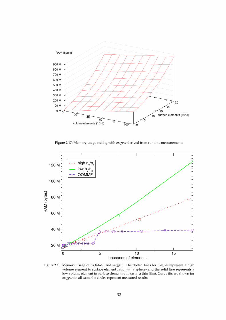
0 20

40 60

80 100volume elements (10^3)

0

5

10

15

20

25

surface elements (10^3)

0 M

100 M

200 M

300 M

400 M

500 M

600 M

700 M

800 M

900 M

RAM (bytes)

Figure 2.17: Memory usage scaling with magpar derived from runtime measurements

0 5 10 15thousands of elements

20 M

40 M

60 M

80 M

100 M

120 M

RA

M (

byte

s)

high nv/n

s

low nv/n

s

OOMMF

Figure 2.18: Memory usage of OOMMF and magpar. The dotted lines for magpar represent a highvolume element to surface element ratio (i.e. a sphere) and the solid line represents alow volume element to surface element ratio (as in a thin film). Curve fits are shown formagpar; in all cases the circles represent measured results.

32

magpar. At this point the problem can now be solved using either a standalone

uniprocessor or symmetric multi-processing workstation, or a clustered supercom-

puter.

Further details can be found in appendix E.

2.9.3 Post-processing

Finally, to visualise the results of the simulation, the magnetisation vector datasets

are transformed from either the OOMMF format or the magpar format to the Vi-

sualisation Toolkit (VTK) format, an open standard for visualisation. These results

are visualised with MayaVi, a piece of data visualisation software initially devel-

oped to assist with the visualisation of computational fluid dynamics environ-

ments. MayaVi depends on VTK.

All of these applications should run in any operating system environment for

which an ANSI-compliant C/C++ compiler is available, however in this project we

have only made extensive use of GNU/Linux and Microsoft Windows machines

running on either Intel or AMD processors.

We have written many other smaller tools to assist with pre- and post-processing

of data files generated by all of the aforementioned applications.

2.9.4 Hardware requirements

Theoretically, these pieces of software have modest hardware requirements, how-

ever as with all simulation problems of this nature “bigger is better”. Ideally, a

machine with a minimum of one gigabyte of RAM should be used to maximise the

size of the potential problem which can be solved.

Each discrete cell within a micromagnetic problem to be solved with

OOMMF consumes approximately one kilobyte of RAM, therefore to solve a sys-

tem with 1 × 106 cells, one gigabyte of RAM is required just to run the simulation.

This is without taking into account the size of the simulation package itself, which

must be loaded into RAM and creates a fixed overhead.

Once operating system overheads are considered, it is clear that the amount of

physical system RAM available to a machine should be greater than the amount of

RAM required by the simulation — this is primarily to avoid “thrashing”, a situ-

ation where the operating system is forced to temporarily write (“swap”) areas of

the RAM to the hard disk and read other areas back into RAM from the disk. The

precise amount of RAM required for operating overheads will vary from system

to system; a system dedicated and optimised for performing only simulations may

only need a few megabytes reserved for the operating environment, but a worksta-

tion which is running other applications concurrently (e.g. visualisation software,

e-mail clients, document editors and Internet web browsers) may require several

hundreds of megabytes.

33

Bearing in mind that the access times in modern hard disks are several orders

of magnitude greater than those of RAM (these access times are measured in mil-

liseconds for hard disk drives and nanoseconds for RAM), this will slow down any

particular simulation by this factor, making successful completion of the simula-

tion impossible from a practical standpoint. Even in an optimised scenario where

data seek latency is eliminated, the hard disk can be expected to deliver data ap-

proximately 100 times more slowly than RAM (Barclay et al., 2003).

The speed at which the processor can perform floating point calculations is

overwhelmingly the primary factor when considering the time a simulation will

take to complete. Any processor which has a fast floating point unit coupled with

a compiler which is able to take maximum advantage of this floating point unit

when optimising the simulation source code is ideal — through our own studies

we note that carefully chosen compiler options can increase the execution speed of

the simulation threefold.

Additional methods such as high-throughput batch processing (Litzkow, 1987,

Litzkow et al., 1988) and clustering (Ridge et al., 1997) allow either sets of simulations

to be performed (e.g. many small computations such as those needed for phase dia-

grams) or larger computations which would be impossible to compute with neither

the memory capacity nor the processing power of a supercomputer. OOMMF, un-

like magpar, is unable to take advantage of the message-passing interface (Snir et al.,

1995, Walker, 1992) common to computational clusters.

2.9.5 Disk space

A collection of large hard disks is also beneficial to allow the long-term storage

of previous simulation runs, assisting with the rapid retrieval of past vector data

created by simulations.

Either 32-bit (single precision) or 64-bit (double precision) floating point num-

bers (IEEE, 1985) can be used to store the components of the vector data. The case

for selecting one precision over another can be argued (Goldberg, 1991) from two

perspectives: storing 32-bit numbers will save disk space if the extra precision of-

fered by 64-bit numbers is not necessary, however vector interpolation used by cer-

tain visualisation techniques (e.g. the calculation of streamlines, figure 2.20) may

benefit from a higher-precision. Further arguments for the use of single or double

precision numbers can be found in Bennett Goldberg (1967), Demmel (1984), Goldberg

(1991) and Knuth (1998). It is worth noting that OOMMF will perform the simu-

lation using double precision numbers irrespective of the precision of the output

format, and the solver component of magpar (Balay et al., 2002, 1997) uses double

precision numbers.

Double precision floating point numbers usually require eight bytes of storage

each. To store the magnetisation vectors for a given mesh in OOMMF, each position

34

of the mesh requires three 64-bit numbers to describe it (x, y and z components).

This gives a simple equation for calculating the amount of space needed to store

one set of magnetisation data for a simulation:

s = a+lxcx

lycy

lzcz

3p

8(2.41)

where a is the space consumed by a header describing the relationship between the

vector data and the simulation, lx, ly and lz represent the size of the complete mesh,

cx, cy and cz are the edge lengths of the discrete cell and p is the number of bits used

to store one floating point number. Note that with OOMMF, even empty cells (i.e.

where |M| = 0) are stored by default.

For example, to store the magnetisation vectors for a sphere of diameter 120nm

(lx = ly = lz = 120 × 10−9m) with a cubic mesh cell size of 5nm3 (cx = cy = cz =

5× 10−9m) with 64-bit precision (p = 64), (120/5)3 ∗ (8 ∗ 3) = 331776 bytes of disk

space are needed, plus a small fixed overhead. If a coarser mesh were used, such

that cx = cy = cz = 10 × 10−9m, then only 41472 bytes of disk space are necessary

to store the magnetisation data for one timestep.

For a complete simulation many sets of magnetisation vector data are stored,

each usually representing a particular “stage” — a point where the magnetisation

configuration for an externally adjustable factor, such as applied magnetic field, is

considered stable. A typical simulation might have 100 of these stages. In the case

of the sphere example above, this equates to over 31 megabytes of disk space. For a

sphere of double the diameter with a high field step resolution (giving 1000 stages

if −500mT ≤ Bx ≤ 500mT and Bx is reduced in 1mT steps), over 2.5 gigabytes of

storage space would be necessary. Doubling the mesh resolution and the diameter

further, such that cx = cy = cz = 2.5nm and d = 480nm, the amount of required

disk space grows to well over 150 gigabytes.

2.9.6 Commodity computing

Although it is possible to perform micromagnetic simulations on a local worksta-

tion, throughput is limited. Having only one CPU means only one simulation

can be effectively performed at one time. When more CPUs are available to use

then more simulations can be performed simultaneously, making parameter de-

pendence studies such as phase diagrams practical.

By configuring several powerful local workstations with MPI (Snir et al., 1995),

it is possible to perform simulations normally impractical; code which can take ad-

vantage of MPI environments such as magpar is capable of using the total available

memory of those MPI-enabled machines effectively as one contiguous block — this

allows larger simulations to be performed.

Condor (Litzkow et al., 1988) provides another mechanism for distributing and

35

computing smaller problems. Whereas high-performance commodity computing

systems such as Beowulf require dedicated compute resources, Condor is designed

to take advantage of the CPU cycles left idle on “normal” workstations. Since these

workstations are not dedicated, the jobs which run on them generally relinquish

their resources when the owner of the workstation returns. Useful results can there-

fore only be acquired if the jobs which run via Condor are capable of completing in

a short time.

Iridis is the University of Southampton’s Linux-based clustered computational

facility, consisting of several hundred Intel and AMD processors. Time is reserved

in advance on this system and scheduling priority organised according to the size

of the job in terms of CPU hours and node availability. As a dedicated compute re-

source it is designed to handle both batch and MPI jobs according to requirements,

however competition for CPU cycles means that only a relatively small proportion

of the total power can be used by an individual.

By using Iridis for extended studies with several variables, Condor for phase

diagrams on smaller samples and optimised local workstation clusters for the most

extreme situations, a varied cross-section of results from the different software can

be acquired.

2.9.7 Visualisation

Visualisation is an important part of scientific computation, both for the analysis of

results and their presentation. To visualise computed results, we use MayaVi (Ra-

machandran, 2001), which makes use of Kitware’s VTK (Schroeder et al., 1996, 1997)

as the middleware for preparing the data prior to being rendered in either POV-Ray

or a Pixar Renderman R© (Pixar, 1989, 2000) compliant raytracer.

We can exploit the features of these tools, particularly by adding features com-

monly found in computational fluid dynamics to further our understanding of the

magnetisation patterns resulting from our simulations.

Figure 2.19 shows a typical visualisation. Point A in the upper image shows the

surface map of a scalar, in this instance the xy angle of magnetisation. For clarity

a wireframe map showing the outline of the finite element mesh is visible. In the

lower image, the scalar surface map remains, though it is translucent (point B). The

cones indicated by point C represent the mean magnetisation of the small area im-

mediately surrounding the cones; the colour shows a scalar (the z component of

the magnetisation) and the direction of the cone reflects the magnetisation vector

itself. Where smaller cones are present in a visualisation, these represent an inter-

polation of the vector where source data is only available around that point rather

than at the point itself. This usually takes place at boundaries, arising from a linear

interpolation between M and 0.

To highlight points of interest, an isosurface of a scalar (such as that indicated

36

zM

−3.14

xy angle

3.14

0

1

A

B

C

D

E

Figure 2.19: A visualisation showing a surface map (A), translucent surface map (B), area mean mag-netisation vectors (C), isosurface (D) and streamlines (E)

37

Figure 2.20: Vortex at the core of a droplet object (see section 5.5) highlighted with streamlines (mass-less particles, or tracers) injected into the material. At the edges of the sample thesefollow the magnetisation as if it were a velocity field; at the core these follow the curl ofthe magnetisation.

by point D) may be shown. The isosurface in this example is again based on the z

component of the magnetisation and attaches a visual representation to the core of

a vortex. Finally, point E shows streamlines, which are the result of tracer particles

being “dropped” into the system. These tracers follow the path of the magnetisa-

tion and provide a visual cue for interesting features of the visualisation; here they

gradually follow the magnetisation around the surface of the sample, spiralling in

until they reach the vortex core.

Where the volume of the sample is of particular interest, a random point mask

can be applied to the visualisation, such as that in figure 2.20. Here streamlines

have again been used to add depth to the visualisation and by operating on a de-

rived vector (in this case, the curl of the magnetisation) the bounds of the vortex

core are clear.

Python (van Rossum, 2003) and Linux shell scripts (Ramey, 2003) were employed

extensively in coordinating the process to take raw simulation results and pro-

duce camera-ready images and animations suitable for the analysis of magnetic

microstructures.

Schematic drawings are occasionally used to assist understanding physical ge-

ometry or aspects of magnetisation. Figure 2.21 shows two schematics of a generic

sample with arbitrary shape and a symmetry in the xy plane (point A), here repre-

38

x

y

z

B B

C

D

A

Figure 2.21: Schematic of out-of-plane (left) and in-plane (right) vortices. The dotted red arrow indi-cates the vortex core direction; the solid blue arrows show the magnetisation circulatingaround the core

10

00

nm

Figure 2.22: A schematic representation of non-patterned media is shown on the left, such as thatused in traditional hard disk media (Albrecht et al., 2003, Suß, 2002); the thicker line de-limits one bit. The representation shown on the right is that of patterned media witheach “dot” containing a single bit

sented by a rhombus. The axes on the left indicate the three-dimensionality of the

sample. If the applied field (point B) were initially applied along the x direction,

then two possible vortex types emerge. The vortex shown in the left sample has

an out-of-plane vortex, where the magnetisation circulates in the xy plane (point C,

solid blue arrow) and the core of the vortex (point D, dotted red arrow) points per-

pendicular to this symmetric plane, i.e. in z. The vortex shown in the right sample

has an in-plane vortex — the circulation of the magnetisation (point C, solid blue

arrow) is in the yz plane and the core of the vortex (point D, solid red arrow) is

aligned with the direction of the initial applied field, i.e. in x.

2.10 Applications

Micromagnetic modelling is important to understand the behaviour of modern

hard disk media and the research of novel materials and designs which could be

incorporated into future hard disk platters.

Other emerging applications such as magnetic RAM can also benefit greatly

from the investigation of micromagnetic systems offered through simulation tech-

niques.

39

2.10.1 Patterned and non-patterned media

Most modern hard disk drives have non-patterned media platters. The platter con-

sists of a substrate, usually made of glass (though in the past aluminium and mag-

nesium have been used), and is plated with nickel-phosphorous. On top of this

substrate a magnetic cobalt-chromium-platinum-tantalum (CoCrPtTa) film is de-

posited by evaporation. This results in an irregular structure approximated in fig-

ure 2.22; the sizes of the individual grains within this structure are approximately

20nm in size (IBM, 2002), though the grain size in the most recent disks is around

5mn (de Groot, 2005). When pieces of data are written to this film, they are written

along tracks shown by the dashed lines in the figure; the magnetisation of the crys-

tals within the area representing that bit is set to a binary state. When the pieces of

data are read back, the drive takes a mean of the magnetisation as measured by the

head and decides whether that particular segment should be a ‘zero’ or a ‘one’, i.e.

a bit of data. Typically, one bit is made up of 20 grains by 50 grains, giving a total

physical bit size of 400nm × 1000nm (0.4µm× 1µm) (IBM, 2002). Figure 2.1 shows

the relationship between bit size and storage capacity.

Advancements in hard disk drive technologies have allowed capacity and per-

formance increases in a similar order of magnitude to that of computer processors

— traditionally doubling approximately every eighteen months but recently ev-

ery twelve months; for example, the giant magnetoresistance (GMR) effect discov-

ered in 1988 (Baibich et al., 1988) gave manufacturers a head technology capable of

reading smaller physical data bits on account of their increased sensitivity. Subse-

quently, to increase data density, manufacturers can reduce the width of the tracks;

at 6 Gbit/in2 this is approximately 1µm.

At some point it becomes impossible to reduce the track width any further

whilst ensuring reliability, and consequently data integrity, as there are too few

CoCrPtTa grains within the track width to guarantee a particular overall state (i.e.

zero or one); a very narrow track may reduce the strength and therefore the “clar-

ity” of the read signal. To increase reliability, manufacturers must reduce the size

of the particles which coat the substrate, thereby increasing the relative number of

grains representing one state; if these particles fall below a certain critical size, the

superparamagnetic effect may reverse the magnetisation in individual grains due

to thermal fluctuations.

Patterned magnetic arrays (Ross, 2001) at a nanoscopic level are becoming fea-

sible as hard disk storage media (Chou, 1997, Chou et al., 1996) owing to advance-

ment in fabrication processes (Cowburn et al., 1999a,b), including self-assembly tech-

niques (Bartlett et al., 2003a, Hoinville et al., 2003, Mayes et al., 2003, Zhukov et al.,

2004a, 2003). However, to understand what precisely should be assembled, a study

is needed into the relative merits of the entities making up the array; indeed, as

nanoscopic length scales are approached, the physical shape of an entity becomes

40

Figure 2.23: A depiction of how data can be accessed in MRAM; light blue areas represent the readpath. Between the purple tracks, from top to bottom: free ferromagnet (yellow), tunneljunction (dark blue), pinned ferromagnet (green), antiferromagnet (red), seed layer (darkgreen)

more important (Aharoni, 2000, p115) than other factors, such as magnetocrystalline

anisotropy, because it will affect increasingly the characteristics of the hysteresis

loop (see section 2.8.1). In chapter 5 we investigate the properties of such nanodots.

2.10.2 Magnetoresistive random access memory

In 1974 IBM Research developed the magnetic tunnel junction, the main component

of magnetostatic random access memory (MRAM). This tunnel junction is a sand-

wich of ferromagnetic and antiferromagnetic material between columns of bits and

rows of words, allowing an “[x, y]”-like access to individual bits within the mem-

ory; this can be seen in figure 2.23.

MRAM has the potential to be fast and dense, but even more importantly, it

is non-volatile i.e. it does not require a constant application of power to retain

its state), unlike standard dynamic random access memory (DRAM). This non-

volatility provides another benefit in the form of low-power consumption, mak-

ing MRAM ideal for applications where power is paramount, such as laptop and

palmtop computers, mobile telephones and portable music systems.

To help understand which particle shapes are useful as part of a typical MRAM

configuration (Teherani et al., 1999), it is beneficial to study these through simulation.

41

Chapter 3

Basic geometries: flat cylinders

and spheres

3.1 Introduction

The knowledge which can be acquired from micromagnetic simulation reveals the

underlying physical processes that govern the hysteresis loop. This complements

experimental work in which the average magnetisation as usually shown in hys-

teresis loops is observed.

The ability to examine numerically the micromagnetic behaviour of a given fer-

romagnetic system is of particular interest to experimentalists because it allows us

to investigate in great detail the microstructures of the magnetisation which form

inside the system and observe their effects.

We wish to understand the micromagnetic behaviour of the droplets later pre-

sented in chapter 5 which our collaborators in Prof. Bartlett’s group can fabricate

and our collaborators in Prof. de Groot’s group investigate experimentally. In this

chapter we study some more fundamental geometries to prepare this investigation.

3.2 Prior work

Previous work with flat cylinders, i.e where the diameter of the circular plane is sig-

nificantly larger than the height, has been done by Cowburn et al. (1999a,b). These

papers present hysteresis loops and SEM micrographs for supermalloy

single-domain circular nanomagnets (flat cylinders). The diameter d of these cylin-

ders is between 55nm and 500nm, and their height h is between 6nm and 15nm.

Cowburn concludes that there is a distinct behaviour switch between the vortex

state and the single-domain state (see figure 3.1) dependent on the diameter of

the nanomagnet, confirmed by micromagnetic simulation (Dao et al., 2001). Two-

dimensional simulation studies by Gubbiotti et al. (2002) show the vortex behaviour

in circular permalloy dots of diameter 200nm. Other single-domain to vortex state

42

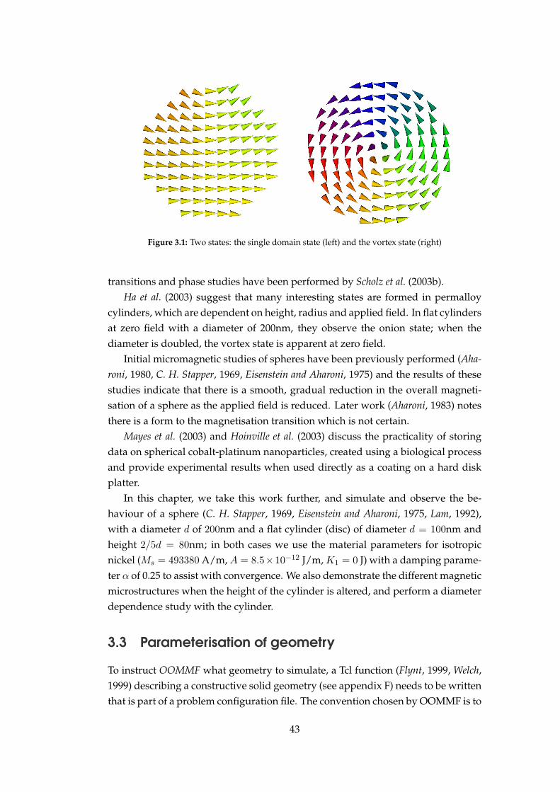
Figure 3.1: Two states: the single domain state (left) and the vortex state (right)

transitions and phase studies have been performed by Scholz et al. (2003b).

Ha et al. (2003) suggest that many interesting states are formed in permalloy

cylinders, which are dependent on height, radius and applied field. In flat cylinders

at zero field with a diameter of 200nm, they observe the onion state; when the

diameter is doubled, the vortex state is apparent at zero field.

Initial micromagnetic studies of spheres have been previously performed (Aha-

roni, 1980, C. H. Stapper, 1969, Eisenstein and Aharoni, 1975) and the results of these

studies indicate that there is a smooth, gradual reduction in the overall magneti-

sation of a sphere as the applied field is reduced. Later work (Aharoni, 1983) notes

there is a form to the magnetisation transition which is not certain.

Mayes et al. (2003) and Hoinville et al. (2003) discuss the practicality of storing

data on spherical cobalt-platinum nanoparticles, created using a biological process

and provide experimental results when used directly as a coating on a hard disk

platter.

In this chapter, we take this work further, and simulate and observe the be-

haviour of a sphere (C. H. Stapper, 1969, Eisenstein and Aharoni, 1975, Lam, 1992),

with a diameter d of 200nm and a flat cylinder (disc) of diameter d = 100nm and

height 2/5d = 80nm; in both cases we use the material parameters for isotropic

nickel (Ms = 493380 A/m, A = 8.5×10−12 J/m, K1 = 0 J) with a damping parame-

ter α of 0.25 to assist with convergence. We also demonstrate the different magnetic

microstructures when the height of the cylinder is altered, and perform a diameter

dependence study with the cylinder.

3.3 Parameterisation of geometry

To instruct OOMMF what geometry to simulate, a Tcl function (Flynt, 1999, Welch,

1999) describing a constructive solid geometry (see appendix F) needs to be written

that is part of a problem configuration file. The convention chosen by OOMMF is to

43

Figure 3.2: Anisotropic simulation domain. The image on the left has the physical x, y and z com-ponents of the simulation domain equal to each other — as such the inscribed geometryis a sphere — while the image on the right has the physical z component half the size ofthe physical x and y components, causing the inscribed geometry to be ellipsoidal. Bothinscribed geometries are described by equation F.1

always operate in a geometric simulation space with internal coordinates ranging

from 0 to 1 in all three dimensions (see figure 3.2). In addition, OOMMF requires

knowledge about the absolute size of this simulation cell and will scale the nor-

malised cell accordingly.

We have found this approach counterintuitive at times and have therefore writ-

ten a Python program (mifmaker) which takes the size of the object we wish to in-

vestigate in absolute units, and will then create the necessary configuration file for

OOMMF automatically, including the Tcl function to describe the geometry in nor-

malised units. To generate a problem which will simulate a cobalt cylinder of di-

ameter 100nm and height 40nm, with a mesh resolution of 2.5nm and an in-plane

applied field ranging from 500mT to -500mT in 1mT steps, we need to issue the

following command to mifmaker:

mifmaker --cylinder --material=cobalt --xy=100e-9 -z 40e-9 \

-c 2.5e-9 -h 500 -l -500 -s 1000 --direction=down

The investment in creating this “one-shot” approach to generating micromag-

netic problems pays off when the parameter space is to be explored systematically.

When OOMMF interprets the problem configuration file, it tests each point in

the normalised geometric simulation space against the geometry function. At this

point, the function can return results of either Ms or zero, depending on whether

or not material is present at the point of test. By inverting the results when the

conditions are met, negative geometries can be built up, such as the “antisphere”

44

-100 -50 0 50 100applied field B

x (mT)

-1

-0.5

0

0.5

1

ma

gn

etisa

tio

n M

xa

c

b

Figure 3.3: Hysteresis loop for a flat nickel cylinder of height 40nm and diameter 200nm. The pointson the graph correspond to the states described in the text and figures 3.5, 3.7 and 3.8

— a spherical hole in an otherwise solid (cubic) geometry.

3.4 Flat cylinder

We compute a hysteresis loop as shown in figure 3.3 in the following way: initially,

a magnetic field is applied in the simulation such that the magnetisation across the

cylinder is homogeneous (see figure 3.4).

For Bx = 0mT (point a in figure 3.3) the magnetisation appears roughly homo-

geneous (figure 3.5) but closer inspection (figure 3.6) reveals a slight out-of-plane

magnetisation shift at either end of the sample due to a small contribution from the

dipolar interaction. This can also be seen in figure 3.5 (Bertram, 1994), and over-

all an onion state occurs, present to minimise the dipolar surface charges (Ha et al.,

2003); this is shown in figure 3.6, and the homogeneous magnetisation state at this

point can be seen with a normalised colour scale in figure 3.5 and corresponds to

point a in figure 3.3.

As the applied field is reduced further a vortex forms in the x-y plane (fig-

ure 3.7). Note that this vortex (point b in figure 3.3) does not appear until after

the applied field has passed zero; the vortex appears here as there is an energy

barrier which it must first overcome. This results in the vortex forming slightly

off-centre, so that when the vortex is created the magnetisation jumps from a high

45

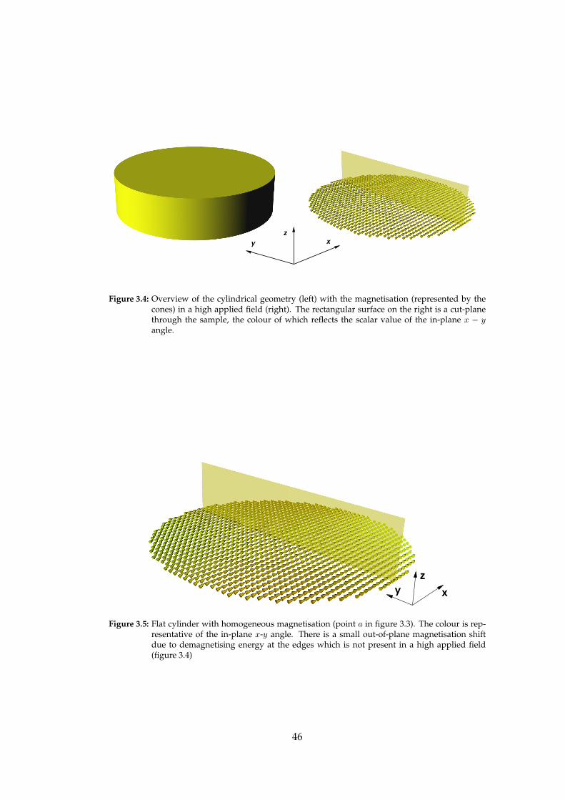
y

z

x

Figure 3.4: Overview of the cylindrical geometry (left) with the magnetisation (represented by thecones) in a high applied field (right). The rectangular surface on the right is a cut-planethrough the sample, the colour of which reflects the scalar value of the in-plane x − yangle.

x

z

y

Figure 3.5: Flat cylinder with homogeneous magnetisation (point a in figure 3.3). The colour is rep-resentative of the in-plane x-y angle. There is a small out-of-plane magnetisation shiftdue to demagnetising energy at the edges which is not present in a high applied field(figure 3.4)

46

−1

1

−1 1z component of magnetisation

y c

om

po

ne

nt

of

ma

gn

etisa

tio

n

x

y

z

Figure 3.6: The flower state and the onion state shown together in a cylinder of diameter 200nm andheight 40nm in zero applied field. The flower state is shown by the coloured cut-plane(xz) and exists in the x-z plane. The onion state is shown by monochrome streamlineswhich follow the magnetisation direction; this exists in the x-y plane.

positive value to approximately −0.1MS , where Ms is the saturation magnetisation

(see figure 3.5). The position of the core of the vortex is a reflection of the amount of

magnetisation which is following the applied field to minimise the Zeeman energy.

As the field is further reduced, the core of the vortex can be seen to pass through

the cylinder in the negative y direction until Mx = −0.7Ms (figure 3.8), correspond-

ing to point c in figure 3.3; at this point the core of the vortex is close to the edge of

the cylinder and disappears with another increase in the magnitude of the applied

magnetic field, leaving the magnetisation once more homogeneous in the direction

of the applied field, which is the opposite situation to that in figure 3.5.

Taking a cylinder of diameter 200nm, we study the microstructures of the mag-

netisation which form for different heights of a cylinder between 5nm and 100nm.

Using the technique outlined in section 2.7.2 we assign a uniform magnetisation in

the x direction, allow the system to relax in zero applied field, and make observa-

tions.

Figure 3.9 shows the flower state, clearly visible in the shorter cylinders; how-

ever as the height is increased, the dipolar energy exerts a greater influence, as in

figure 3.6. The dipolar energy continues to exert more and more pressure on the

cylinder to abandon its flower state in favour of a vortex — at a height of 75nm

the top and bottom of the cylinder are completely dominated by the magnetostatic

47

x

z

y

Figure 3.7: Flat cylinder entering the vortex state (point b in figure 3.3). The direction of the conescorresponds to the direction of the magnetisation; their colour shows their angle in thex-y plane — yellow is 0◦ from +x, blue is 180◦ from +x. The translucent cutplane iny-z shows the magnetisation pattern is consistent throughout the height, and the greyisosurface outlines the core of the vortex.

x

z

y

Figure 3.8: Flat cylinder just before leaving the vortex state (point c in figure 3.3).

Figure 3.9: Height dependence of the remanent state in cylinders - vertical cutplanes in the xz planeof a cylinder of diameter 200nm in zero applied field are shown. The images are (left) acylinder of height 35nm, (centre) h =75nm and (right) h =85nm. The colour variationrepresents the z component of the magnetisation.

48

60 80 100 120 140 160Diameter (nm)

20

40

60

80H

eig

ht (n

m)

single-domain state

vortex/multi-domain state

Figure 3.10: Phase diagram of the remanent magnetisation state for nickel cylinders of varying heightand diameter

energy. Increasing the height a little further from here to 80nm causes this structure

to collapse and fall into the vortex state at zero field.

Figure 3.10 shows the reversal behaviour of nickel cylinders dependent on height

and diameter. As height is increased, the single domain behaviour disappears and

vortex reversal behaviour occurs; the same is true as the diameter is increased.

3.5 Sphere

3.5.1 Finite differences and finite elements

Figure 3.11 depicts the hysteresis loops obtained from simulations of a nickel sphere

(diameter d=200nm, K1=0). The loops in the upper left, upper right and lower left

of the figure show loops yielded with the OOMMF software, whilst the lower right

loop was computed with magpar.

For each simulation, the applied field direction was varied in θ and φ, respec-

tively the azimuth and polar angle of the applied field. These are relative to the

orientation of the finite difference grid, aligned with the x-, y- and z-axes.

All the loops show a similar pattern just below saturation, with small openings

in the hysteresis where the magnetisation moves from the single domain state into

49

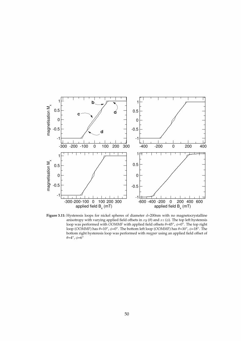
-300 -200 -100 0 100 200 300

-1

-0.5

0

0.5

1

magnetisation M

x

-400 -200 0 200 400

-1

-0.5

0

0.5

1

-300-200-100 0 100 200 300applied field B

x (mT)

-1

-0.5

0

0.5

1

magnetisation M

x

-600 -400 -200 0 200 400 600applied field B

x (mT)

-1

-0.5

0

0.5

1

c

d

a

b

Figure 3.11: Hysteresis loops for nickel spheres of diameter d=200nm with no magnetocrystallineanisotropy with varying applied field offsets in xy (θ) and xz (φ). The top left hysteresisloop was performed with OOMMF with applied field offsets θ=45o, φ=0o. The top rightloop (OOMMF) has θ=10o, φ=0o. The bottom left loop (OOMMF) has θ=30o, φ=18o. Thebottom right hysteresis loop was performed with magpar using an applied field offset ofθ=4o, φ=6o

50

the vortex state.

It is interesting to note that in the loops computed with OOMMF there is an

“opening” in the hysteresis loop around Bx=0, the size of which varies with the

direction of the applied field, although it is never quite eliminated. The results

from magpar do not display this characteristic.

These data show that the inner loop depends on the angles θ and φ. For the

spherically symmetric system that we wish to simulate, how the coordinate system

of the simulation software is aligned relative to the direction of the applied field

should be irrelevant. It is therefore likely that the inner openings in the hystere-

sis loops are an artefact of the finite difference simulation technique as these vary

substantially as a function of this direction.

Initially, we assume the applied field is zero and the magnetisation forms a vor-

tex with the core pointing in the x direction as shown later in figure 3.15, and a very

small field is applied in the opposite direction (i.e. −x) such that the vortex struc-

ture of the magnetisation is not significantly affected. Since the overall magnetic

moment of the magnetisation is finite and points in the direction of the moments

in the vortex core, it is therefore energetically favourable for the system to align the

vortex core with the applied field.

In order for this to happen, the vortex core needs to turn around by 180 degrees

(i.e. point in −x rather than +x. If there is no magnetocrystalline anisotropy in the

system, the spherically symmetric sphere should allow the core to rotate round in

either θ or φ, similar to a typical Stoner-Wohlfarth particle. The spherical symmetry

should not allow the occurrence of the “inner” hysteresis loop indicated in figure

3.11; this is supported by the results presented in the lower right of figure 3.11

computed with the finite element code.

It is plausible therefore to assume that directions along the discretisation axis are

either favoured or avoided by the system when a finite difference grid is introduced

for symmetric geometries.

3.5.2 Reversal mechanism

A strong magnetic field applied across a nickel sphere of diameter 200nm gives a

homogeneous magnetisation. As this field is reduced the magnetisation at the sur-

face of the sphere diverges as a consequence of the dipolar interactions (figure 3.12

corresponding to point a in figure 3.11; also shown in figure 3.13); this behaviour is

similar to that in small cylinders.

As the field is reduced, the sphere falls into the vortex state a little above 100mT

(see figure 3.14, corresponding to point b in figure 3.11), but, contrary to the cylin-

der, this vortex forms around the axis of the applied field. The majority of the mag-

netisation at this stage is pointing in the direction of the applied field rather than

against it, as the core of the vortex is aligned with the direction of the initial mag-

51

z

xy

z

xy

Figure 3.12: Nickel sphere in high applied field showing spin tapering owing to demagnetising en-ergy; the left image shows a cut-plane through x and y, the right image shows a cut-planethrough x and z. This corresponds to point a in figure 3.11

netisation. The magnetisation around the core of the vortex is able to maintain its

circular vortex pattern and adjust its alignment with the present applied field.

At zero field, the magnetisation in the vortex core remains pointing in the di-

rection of the applied field (figure 3.15, corresponding to point c in figure 3.11),

however if the field is increased in the −x direction then the magnetisation in the

core is reversed (figure 3.16, point d in figure 3.11).

Further increasing the field eventually results in the vortex dissipating at around

180mT. This results in the magnetisation of the sample pointing entirely in the di-

rection of the applied field as in figure 3.13, only in the opposite direction.

3.5.3 Size dependence

A size dependence study was performed on the diameter of nickel spheres; the

results of this can be seen in figure 3.17, showing a change in behaviour at a certain

diameter.

There is a qualitative change in the magnetisation reversal when the diameter

is reduced; the hysteresis loops for spheres of diameter 50nm and 80nm are shown

in figure 3.18.

The following equation (O’Handley, 1999) gives the critical radius (i.e. the radius

above which a sphere changes from single domain behaviour to vortex behaviour)

of a spherical sample of some material which has a low anisotropy value.

rn+1 =

√

9A

µ0M2s

[

ln

(

2rna

)

− 1

]

(3.1)

Using this equation, one can quickly converge on the critical radius for nickel by

iterating equation 3.1 until rn+1 − rn = 0. The calculated critical radius of 34nm

agrees well with our simulations of nickel spheres; these studies show that the

magnetisation pattern of a nickel sphere of diameter 60nm (r = 30nm) reverses

52

y xz

Figure 3.13: Sphere at high applied field (point a in figure 3.11); see also figure 3.12.

y xz

Figure 3.14: Sphere immediately after entering the vortex state (point b in figure 3.11).

53

y xz

Figure 3.15: Sphere in vortex state (point c in figure 3.11).

y xz

Figure 3.16: Sphere in vortex state at a further reduced field (point d in figure 3.11).

54

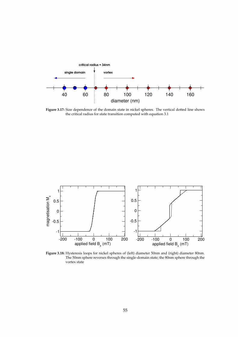
40 60 80 100 120 140 160

diameter (nm)

vortexsingle domain

critical radius = 34nm

Figure 3.17: Size dependence of the domain state in nickel spheres. The vertical dotted line showsthe critical radius for state transition computed with equation 3.1

-200 -100 0 100 200applied field B

x (mT)

-1

-0.5

0

0.5

1

magnetisation M

x

-200 -100 0 100 200applied field B

x (mT)

-1

-0.5

0

0.5

1

Figure 3.18: Hysteresis loops for nickel spheres of (left) diameter 50nm and (right) diameter 80nm.The 50nm sphere reverses through the single-domain state; the 80nm sphere through thevortex state

55

as a single-domain, and the magnetisation pattern when the diameter is 70nm is

vortex-like.

3.6 Summary

We have studied the magnetisation reversal in nickel cylinders and spheres of the

size order 200nm. Around this size, in nickel the samples will not tend to form

domain walls as the samples are physically too small — the energy from dipolar

interaction is not great enough to counteract the domain wall energy — and neither

will the shapes behave as single-domain states as the dipolar energy is then too

great (Wachowiak et al., 2002).

Below a certain critical diameter, cylinders exhibit single-domain behaviour.

Above this critical diameter, the cylinders enter the vortex state. In this regime,

the vortex penetrates and moves to adapt Mx to Bx after the field is reversed. In

all cases, nickel cylinders cannot maintain a single-domain reversal method once

their height is above a critical value; we find that the vortex reversal method is

present in all cylinders with a height greater than 60nm. The results for the simu-

lated cylinders are qualitatively in agreement with work by Cowburn et al. (1999b),

however these cannot be compared directly because different materials have been

investigated.

With the simulated spheres, vortex behaviour exists for a sufficiently large sys-

tem, however the vortex penetrates at a greater applied field than that in a cylinder

of comparable size. The vortex in spheres is also static with the core of the vortex

pointing in the original direction of the applied field, as opposed to the vortex ap-

pearing in cylindrical samples, where the core of the vortex is able to move through

the system to compensate for a change in applied field. In cylindrical samples, the

core of the vortex is perpendicular to the direction of the applied field, i.e. it points

out of the circular plane.

We have shown that for non-cuboidal structures, great care has be taken to en-

sure that the finite difference simulation technique does not introduce artefacts that

do not reflect the behaviour of the physical system. In subsequent chapters we have

used finite element simulations to corroborate finite difference simulation results,

and varied the directions of applied field to ensure to exclude such artefacts from

our observations.

56

Chapter 4

Cones

The work described in this chapter has been submitted to Physical Review B (Board-

man et al., 2005a).

4.1 Introduction

Tapered structures such as pyramids and cones are commonly used in magnetic

force microscopy (Dahlberg and Proksch, 1999, Saenz et al., 1987); the phase shift in-

duced by the movement of a cantilever attached to the structure can be interpreted

to yield the stray field pattern of a sample (McVitie et al., 2001).

Part-conical samples of size order 1µm and above have previously been fabri-

cated for bubble devices (Sanders et al., 1981). Nanolithographically defined struc-

tures created through electron beam lithography (Chou, 1997, Chou et al., 1996) re-

sult in arrays of tapered pillars which are geometrically conical. The coercivity of

arrays of shorter cones created with interference lithography has been previously

investigated experimentally and numerically (Ross et al., 2001).

In this chapter, we study the magnetic reversal behaviour of cones systemati-

cally and compute a magnetisation remanence phase diagram as a function of di-

ameter and height.

4.2 Parameters

We use the material parameters for Ni80Fe20 permalloy (Js = 1.0 T, A = 1.3×10−11

J/m, K1 = 0.0 J/m3) (Skomski and Coey, 1999) and a damping constant α of 0.25 to

improve convergence.

We perform simulations on cones where the overall diameter d of the base

ranges from 10nm to 100nm, the height h between the base and the tip ranges from

10nm to 100nm and the external magnetic field is applied along the x direction of

the cone (see figure 4.1).

57

xy

z

single domain x single domain z buckle state C state out−of−plane vortex

d

h

Figure 4.1: Representation of remanent magnetisation states; the solid arrows indicate the magnetisa-tion direction, the dotted arrow shows the vortex core direction. From left to right: singledomain state in x, single domain state in +z (filled arrow) and −z (hollow arrow), bucklestate (Koltsov et al., 2000), C state and out-of-plane vortex state.

The mesh for the magpar hybrid FE/BE simulation is created using NETGEN

(Schoberl, 2003). For the cone where d = 100nm and h = 100nm, the mesh contains

210825 tetrahedra, with the largest element having an edge length smaller than

4nm, which is below (Donahue and McMichael, 1997) the calculated exchange length

λex =√

2A/µ0M2s (Kronmuller and Fahnle, 2003) of 5.71nm.

The remanent magnetisation configurations using OOMMF and magpar are in

agreement providing the shape is sufficiently well resolved in both cases. To ensure

this is the case with OOMMF, the cones were discretised into 8000 cells, in the

largest case the cell edge length is 5nm with a maximum adjacent cell spin angle of

0.5 radians.

Starting from an initially uniform magnetisation state pointing in the +x direc-

tion, we apply a magnetic field of 500mT capable of maintaining a nearly homoge-

neous magnetisation and reduce this field in steps of 1mT until the magnetisation

is reversed to compute the hysteresis loop. When the applied field is reduced to

zero, we classify the magnetisation pattern to create the remanence phase diagram.

Figure 4.1 shows schematic plots of the observed remanent states.

4.3 Results

Figure 4.2 shows the phase diagram for the remanent magnetisation states in cones

where 10nm ≤ d ≤ 100nm and 10nm ≤ h ≤ 100nm and the applied field was orig-

inally in the +x direction (see figure 4.1). Where h is less than 20nm, the remanent

state is a single domain state with the magnetisation pointing in the x direction

(figure 4.1, left). If h is above 50nm and the ratio h/d is high (i.e. a tall, thin cone)

then the single domain state in z is preferable due to shape anisotropy (figure 4.1,

second from left). We have observed two types of single domain states in z: one

with the magnetisation pointing up towards the tip of the cone and the other with

the magnetisation pointing down towards the base. The single domain states in x

58

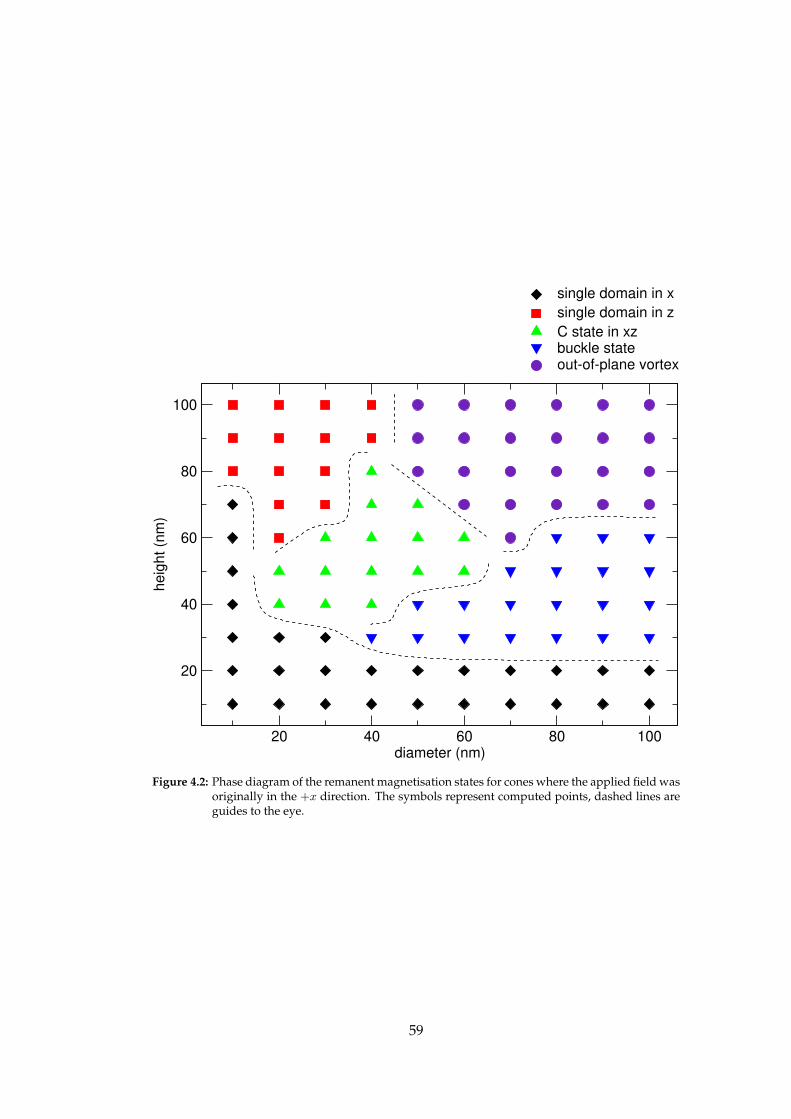
20 40 60 80 100diameter (nm)

20

40

60

80

100

heig

ht (n

m)

single domain in x

single domain in z

C state in xzbuckle stateout-of-plane vortex

Figure 4.2: Phase diagram of the remanent magnetisation states for cones where the applied field wasoriginally in the +x direction. The symbols represent computed points, dashed lines areguides to the eye.

59

-300 -200 -100 0 100 200 300applied field B

x (mT)

-1

-0.5

0

0.5

1

ma

gn

etisa

tio

n M

x

A

D

C

B

x

z

y

EF

G

H

Mx−1.0 1.0

Figure 4.3: Hysteresis loop and reversal mechanism for a cone where d = h =100nm and the appliedfield is across the diameter. Points E, F, G and H are explained in figure 4.4.

and z are in agreement with experimental data in Ross et al. (2001).

For larger h and d the demagnetising energy grows and the remanent state is

the vortex state with the magnetisation in the core of the vortex pointing out of the

xy plane (figure 4.1, right).

For intermediate values of h we find at large d the buckle state (figure 4.1, cen-

tre), in which the overall magnetisation points in x but around the centre of the xy

plane this bends slightly upwards and downwards in z. The buckling is an indica-

tion of the growing dipolar energy of the single-domain state.

At smaller d for intermediate h the remanent state is a C-shaped configuration

(figure 4.1, second from right). The C state is related to the single domain state in

z by the shape anisotropy driving the magnetisation to point primarily in the -z

direction. In larger diameters the magnetisation will attempt to reduce the demag-

netisation energy — the bending of the magnetisation in the +x direction close to

the base of the cone shows the history of the system: prior to the field being reduced

to zero the magnetisation was pointing in the +x direction.

Figure 4.3 shows the complete hysteresis loop for a cone with d=h=100nm, com-

puted using magpar. When the applied field is reduced from saturating the mag-

netisation in the +x direction, it forms an in-plane vortex (i.e. where the mag-

netisation circulates in yz and the vortex core points in the x direction) shown at

point A. The same behaviour is observed for the magnetisation reversal of spheres

60

(Boardman et al., 2005b, Eisenstein and Aharoni, 1975) of similar size. Note that this

configuration is not observed in the absence of an applied field and therefore this

state is not shown in figure 4.1.

The in-plane vortex is replaced by an out-of-plane vortex (i.e. where the mag-

netisation circulates in xy and the vortex core points in the z direction) shown at

point B after overcoming an energy barrier. The core of this vortex is anchored at

the tip of the cone and compensates for the applied field by tilting the core, allowing

the majority of the magnetisation to align with the applied field, thus minimising

Zeeman energy.

A further reduction of the field (point C) causes the core of the vortex to shift to

the centre of the cone. Reducing the field below zero causes the vortex to bend in

the opposite direction to point B. At Bx = 0mT the magnetisation is in the vortex

state as shown in figure 4.1 (right). Another energy barrier needs to be overcome to

destroy the out-of-plane vortex, leaving the magnetisation with an in-plane vortex

(point D) with the core pointing in the opposite direction to the vortex at point A.

Once the field is sufficiently high the in-plane vortex aligns into a homogeneous

saturated magnetisation in the -x direction for |Bx| ≥ 250mT.

Figure 4.4 shows specifically the magnetisation at points E, F, G and H from

figure 4.3 to explain the subtle “kinks” in the hysteresis loop. The top row shows

a magnetisation cross section along the height of the cone and the bottom row that

along the base. The middle row is a schematic representation of the two vortices

corresponding to the cross sections above and below.

Starting at point E, the system contains two vortices: the out-of-plane vortex

with the core pointing in the +z direction introduced at point B, and the formation

of an in-plane vortex with the core in the -x direction parallel to the applied field.

Increasing the field in the -x direction causes the in-plane vortex to become more

dominant (point F). A further increase of the applied field in the -x direction allows

the in-plane vortex to become even more influential, moving the out-of-plane vor-

tex to the edge of the sample (point G). There is a small energy barrier present to

force the out-of-plane vortex from the system; once this has been overcome only

the in-plane vortex remains (point H).

4.4 Summary

We have simulated the magnetisation reversal in conical samples, and five separate

remanent states — single-domain in x, single-domain in z, out-of-plane vortex,

buckle and C-state — have been observed.

By analysing the remanent magnetisation configuration for a series of simula-

tions, we have created a phase diagram showing these results. The dynamics of the

magnetisation reversal are more complicated to classify and describe.

61

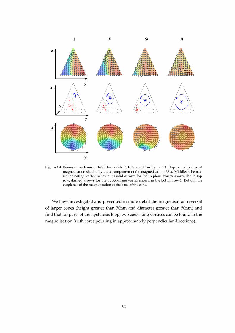
z

y

x

y

z

y

x

E F G H

Figure 4.4: Reversal mechanism detail for points E, F, G and H in figure 4.3. Top: yz cutplanes ofmagnetisation shaded by the x component of the magnetisation (Mx). Middle: schemat-ics indicating vortex behaviour (solid arrows for the in-plane vortex shown the in toprow, dashed arrows for the out-of-plane vortex shown in the bottom row). Bottom: xycutplanes of the magnetisation at the base of the cone.

We have investigated and presented in more detail the magnetisation reversal

of larger cones (height greater than 70nm and diameter greater than 50nm) and

find that for parts of the hysteresis loop, two coexisting vortices can be found in the

magnetisation (with cores pointing in approximately perpendicular directions).

62

Chapter 5

Nanodots

The work described in this chapter has been published in two papers in the Journal

of Applied Physics (Boardman et al., 2004, 2005b).

5.1 Introduction

Figure 5.1 shows an array of nanodots created using the novel “double template”

method imaged using a scanning electron microscope.

Figure 5.2 shows the experimentally measured hysteresis loop for such an ar-

ray of nickel nanodots (see section 5.1.1) with a bounding sphere diameter d of

500nm (Zhukov, 2004) obtained through magneto-optical Kerr effect (Argyres, 1955)

microscopy. The motivation here is to reveal the physics in this hysteresis loop

through micromagnetic simulation.

Although the precise shape of the nanodot is not known, we do know the man-

ufacturing method (see section 5.1.3) and from this we can derive an approximate

representation of the nanodot.

It is not feasible to perform a three-dimensional micromagnetic simulation of a

large array of nanodots so instead a single nanodot is modelled numerically. De-

spite some inevitable dipolar interaction in the real system, particularly when the

nanodots are close together, it remains of interest to investigate the magnetisation

of an independent nanodot.

5.1.1 What is a nanodot?

We define a nanodot to be a magnetic sample with a physical edge size lx of less

than 1µm and “short” in geometry, i.e. lz ≤ 0.5lx. Arrays of nanodots are strong

candidates for use in patterned media, as the consistency of shape from one nan-

odot to the next promotes predictable behaviour; one nanodot will behave in the

same way to another nanodot, in contrast to irregular grains where clusters of

grains are required to reduce the effects of this irregularity.

63

Figure 5.1: Scanning electron microscope image of a droplet array

-200 -100 0 100applied field B

x (mT)

-0.5

0

0.5

1

ma

gn

etisa

tio

n M

x

Figure 5.2: Normalised MOKE measurements for a nickel dot array of diameter 500nm

64

d

water latex spheres

substrate

non−magnetic material

holes

h

magnetic material

Figure 5.3: The double-template self-assembly technique. First, an aqueous suspension of latexspheres (top left) of diameter d is poured onto a substrate. As the water evaporates,the latex spheres are attracted to each other (top centre), forming a regular close-packedstructure. This template can be filled with a non-magnetic material (top right) and thelatex spheres etched away (bottom left). The resulting gaps can be filled with a magneticmaterial to a varying height h (bottom right) to form arrays of connected or disconnectedpart-spherical nanodots.

5.1.2 Lithography

There are several different ways of creating nanodots. Lithographic methods such

as those used by Cowburn et al. (1999a), Li et al. (2002) and discussed in chapter 3,

although successful, are limited in the grain size they can produce; in photolithog-

raphy the wavelength of light used in the fabrication process effectively limits the

dot size to those above 0.4µm, and electron beam lithography is still a prohibitively

expensive process.

5.1.3 Self-assembly

Self-assembly methods (Denkov et al., 1993) appear to be a cost-effective way to

create templates, from which an array of structures as shown in figure 5.1 can be

formed (Ghanem et al., 2004, Zhukov et al., 2003). These structures are the motiva-

tion behind this chapter. One particular method of chemical self-assembly involves

the formation of templates through the evaporation of an aqueous suspension of

polystyrene latex spheres (Bartlett et al., 2002, 2003a), initiating the self-assembly.

Figure 5.3 shows this process schematically.

Using these templates, it is possible to create magnetic structures from sizes of

50nm to 1000nm by filling the spaces between the close-packed spheres with some

material through electrochemical deposition. By etching away the polystyrene

spheres, another template is formed. This template can then be filled with magnetic

65

2/7d

1/7d

dz

x

Figure 5.4: A typical nanodot “droplet” geometry arranged in a hexagonal lattice (artist’s impressionon the left) and a schematic of the droplet (right)

material, and by varying the fill amount of the resulting spherical holes, connected

or disconnected arrays of dots can be formed. This is known as the double-template

self-assembly method.

The resulting structures have several applications, such as photonic materi-

als (Bogomolov et al., 1997, Vlasov et al., 2001), microchip reactors (Gau et al., 1999)

and biosensors (Velev and Kaler, 1999). The application in which we are interested

for this work pertains to magnetism.

We present here the results for two types of nanodot geometry — part-sphere

and “droplet”. The droplet geometry can be considered to be a part-sphere with a

rounded upper; this is described in more detail in section 5.5.

5.2 Half-sphere

We wish to simulate a half-sphere so we can see what effect the rounded upper

dome (which can be seen in figure 5.1) has on the results; these can then be com-

pared to “droplet” systems (section 5.5) which reflect the shape in figure 5.1. The

half-sphere nanodot we simulate here is isotropic nickel (Ms = 493380 A/m, A =

8.5× 10−12 J/m, K1 = 0 J), with a diameter of 200nm. We use OOMMF to simulate

this geometry with a finite difference cubic cell of edge length 5nm.

5.2.1 Results

Applying a sufficiently large magnetic field across the circular plane of a half-

sphere results in an initially homogeneous magnetisation pattern, and as with the

sphere in section 3.5, a slight deviation at the surface resulting from the demagnetis-

ing field. This corresponds to point a in figure 5.5; the homogeneous magnetisation

is illustrated in figure 5.6.

66

-400 -200 0 200 400Applied field B

x (mT)

-1

-0.5

0

0.5

1

No

rma

lise

d m

ag

ne

tisa

tio

n M

x

a

b

c

Figure 5.5: Hysteresis loop for a nickel half-sphere of diameter 200nm

Reducing the field further causes the nucleation of a vortex at around 30mT,

resulting in the magnetisation drop immediately following point a in figure 5.5.

The vortex core moves in the −y direction while the field is reduced further

(point c in figure 5.5; illustrated in figure 5.8), until the vortex leaves the system

and a homogeneous magnetisation in the −x direction is established.

5.2.2 Discussion

Although hysteretically this exhibits a qualitative similarity with the sphere (fig-

ure 3.11) insofar as their possession of two minor loops, the magnetic microstruc-

ture is more reminiscent of the flat cylinder in that the vortex nucleates out of the

plane and moves through the geometry in the same fashion as the flat cylinder (fig-

ures 3.3 to 3.8), however the vortex appears prior to the applied field being reduced

below zero.

Figure 5.7 illustrates that at zero field the direction of the vortex core is perpen-

dicular to and in the centre of the xy plane; see point b in figure 5.5. For isolated

half-spheres we always find the magnetisation in the core of the vortex to point

“down” (i.e. towards the spherical surface). We attribute this to the asymmetry of

the half-sphere in the z direction.

5.3 Part-spherical nanodots

We have seen above that the magnetisation reversal in the half-sphere occurs via

vortex nucleation similar to the mechanism in the flat cylinder shown in section 3.4.

67

xz

y

Figure 5.6: Half-sphere at high applied field (point a in figure 5.5)

Figure 5.7: Half-sphere in vortex state in zero applied field (point b in figure 5.5). Axes are the sameas those in figure 5.6

68

Figure 5.8: Half-sphere in late vortex state (point c in figure 5.5). Axes are the same as those in fig-ure 5.6

We have shown in section 3.5 that a full sphere reverses via a different mechanism.

From this it can be concluded that for some height h > d/2 of a part-sphere a

transition between the two reversal mechanisms takes place.

These results are also relevant to the experimentally manufactured nanodots

because the amount of material that is deposited through the self-assembly method

described in section 5.1.3 can be varied to grow spheres of heights h ≤ d.

We calculate numerically the magnetisation reversal of soft part-spherical par-

ticles. The observed reversal mechanisms range from single domain reversal at

small radii, to vortex movement in shallow systems at larger radii and vortex core

reversal at larger heights as observed in spheres.

In this section we study the behaviour of the new class of part-spherical struc-

tures and compute a magnetic reversal phase diagram as a function of diameter

and height.

5.3.1 Parameters

Geometrically we consider the part-spheres to have one flat surface when h < d; in

the case h = 0.5d the geometry will resemble the half-sphere from section 5.2.

We perform the phase diagram studies using the material parameters for

Ni50Fe50 permalloy (Ms = 1.11×106 A/m, A = 5.85×10−12 J/m, K1 = 0 J/m3, see

also appendix C) and a damping constant α of 0.25 to improve convergence.

69

12.5 25 37.5 50 62.5 75 87.5 100 112.5 125bounding sphere diameter d (nm)

0.2

0.4

0.6

0.8

1

heig

ht (h

/d)

in-plane vortex

perpendicular vortex

single domain

Figure 5.9: Phase diagram of reversal mechanisms for Ni50Fe50 permalloy part-spheres. The dottedand dashed lines are guides to the eye indicating reversal mechanism boundaries

5.3.2 Results

Figure 5.9 shows a phase diagram of remanent magnetisation states for systems

simulated with magpar where the height h increases from 1/8d to d in 1/8d steps

and d varies between 12.5nm and 125nm.

We observe three distinct reversal mechanisms. Taking d=50nm, for h/d ≤ 0.375

the reversal is coherent; all the magnetic moments remain aligned and rotate ho-

mogeneously. Between h/d = 0.5 and h/d = 0.875 an out-of-plane vortex forms

with a core perpendicular to the applied field after some initial energy barrier is

overcome and this can freely move around the inside of the part-sphere with the

applied field. This is similar to the behaviour seen in cylindrical particles shown

in figures 3.3 to 3.8 and in other works (Boardman et al., 2004, Cowburn et al., 1999b,

Ha et al., 2003, Li et al., 2002). We will now discuss the reversal mechanism in more

detail.

Figure 5.10 shows the perpendicular vortex reversal behaviour. Point A shows

the homogeneously aligned state at high applied field, though there is a small C-

state-like shift in the x-z direction at the extremities in order to minimise dipolar

energy. At point B there is a shift into an S-like state in the x-y direction, where

the magnetic moments at the edges of the half-sphere persist in the applied field

direction while the moments towards the centre are aligned a few degrees away

70

-200 -100 0 100 200applied field B

x (mT)

-1

-0.5

0

0.5

1

magnetisation M

x

Mx

xy

z

AB

C

D

E

Figure 5.10: Reversal mechanism for d=50nm, h=0.5d

from the x direction into the y direction. Reducing the field further overcomes

an energy barrier and a perpendicular (i.e. the core of the vortex points in the z

direction) vortex is formed. Point C shows the remanent state of the half-sphere

with this vortex in the centre; the net magnetisation in the x direction is now zero.

Point D shows the effects of a continued field reduction; the vortex has shifted

further into the y direction appropriate for allowing the majority of the magnetic

moments to point in the negative x direction. Finally, at point E the external field is

now sufficiently low to remove the vortex from the system, and a homogeneously

aligned state remains.

Figure 5.11 shows the reversal mechanism with an in-plane vortex for a sphere

(i.e. h/d = 1.0). Although the size and material differ from the sphere in section 3.5,

there is a qualitative similarity we will review. Point A shows a homogeneous

alignment of the magnetic moments in the x direction, which persists until point B,

where the field has been lowered enough to overcome the energy barrier and allow

an in-plane (i.e. where the core points in the x direction) vortex to form; this also

allows the majority of the magnetisation to continue pointing in the x direction.

As the field is further reduced, the x component of the magnetisation outside

the vortex core continues to follow the applied field; however the core remains

pointing wholly in the direction of the initial applied field. At point C, after the

field is reduced below zero the core of the vortex flips over, which is responsible

71

-400 -200 0 200 400applied field B

x (mT)

-1

-0.5

0

0.5

1

magnetisation M

x

z

y x

zM

AB

C

D

Figure 5.11: Reversal mechanism for d=100nm, h=d

for the “minor” hysteresis loop around Bx = 0. The vortex can exit the system

when the field is further reduced and the magnetisation becomes homogeneous

(point D).

Our simulation results agree with the computation of the critical radius

(O’Handley, 1999, p305) of single-domain to vortex state transition (equation 3.1)

for Ni50Fe50 permalloy in spheres of radius 12.4nm (d=24.8nm): a single-domain

remanent state is observed in our simulations of spheres of diameter 24nm and

below where the exchange energy is dominant, whilst an in-plane vortex is in the

remanent state when the diameter is 25nm or greater as the dipolar energy becomes

preponderant.

5.3.3 Comparing OOMMF and magpar

Figure 5.12 shows results computed during the simulation of a half-sphere of diam-

eter 50nm using two different simulation packages that employ the finite difference

method (Donahue and Porter, 1999) and the hybrid finite element/boundary element

method (Scholz et al., 2003a) respectively. There is good agreement between the two

packages.

The results obtained from both OOMMF (FD method) and magpar (hybrid FE/BE

method) display an energy barrier which is overcome when Bx is below 50mT. Ad-

ditionally, reversible behaviour around Bx = 0 is present in both cases.

72

-200 -100 0 100 200applied field B

x (mT)

-1

-0.5

0

0.5

1

ma

gn

etisa

tio

n M

x

finite differencefinite element/boundary element

Figure 5.12: Hysteresis loops for a d=50nm half-sphere obtained with (solid line) OOMMF (finitedifference method) and (dashed line) magpar (finite element/boundary element method)

The slight aberration in the hysteresis loop for the hybrid FE/BE case is caused

by a slight shift in the magnetisation towards the centre of the sample (figure 5.10,

point B), present in the simulation as a result of the improved shape resolution over

the FD case.

5.4 Multiple vortex states

As the diameter of a part-spherical geometry is increased, further characteristics

are observed which resemble those of the full sphere.

Figure 5.13 shows the hysteresis loop for an isotropic nickel half-sphere of di-

ameter 350nm. This hysteresis loop shares some similarity with that of a smaller

half-spherical system, such as that in figure 5.10 — it has zero remanence and there

are openings in the hysteresis loop. The characteristic difference between the two

loops is there are two energy barriers: the first occurs when Bx is around 100mT,

followed by another when Bx is approximately 70mT, corresponding to the kink in

the curve at 60mT in figure 5.10.

Figure 5.14 reveals the magnetic microstructures in this model. The image on

the left shows the magnetisation when Bx is 80mT. An in-plane vortex has formed

and the magnetisation circulates in the yz plane, with the core of the vortex point-

ing in the x direction with the applied field. The image on the right shows the

73

-200 -100 0 100 200applied field B

x (mT)

-1

-0.5

0

0.5

1

ma

gn

etisa

tio

n M

x

Figure 5.13: Hysteresis loop for an isotropic nickel half-sphere of diameter 350nm. Two energy barri-ers can be seen: one at ≈100mT and another at ≈70mT. The first indicates the transitionfrom the single-domain state to the in-plane vortex state, the second the transition fromthe in-plane vortex state to the perpendicular vortex state.

magnetisation after Bx has been reduced to 65mT. The in-plane vortex has been re-

placed by a perpendicular vortex: the magnetisation now circulates in the xy plane

with the core of the vortex pointing in the z direction. The core of the vortex is

off-centre to allow the majority of the magnetisation to point in the direction of the

applied field.

Figure 5.15 shows the hysteresis loop when the diameter of the nickel half-

sphere is increased to 750nm. Qualitatively, the same behaviour is observed as

when the half-sphere diameter is 350nm. Point A shows the fully-saturated mag-

netisation at a high applied field in the +x direction. When this is reduced to over-

come the first energy barrier (point B) then the in-plane vortex forms, with the core

of the vortex pointing in the direction of the applied field. As the field is reduced to

immediately prior to the second energy barrier at around 75mT (point C), the mag-

netisation around the core of the vortex deviates further away from the x direction

to minimise dipolar energy.

Point D shows the magnetisation immediately after the second energy barrier

has been overcome. The in-plane vortex has disappeared to be replaced by a per-

pendicular vortex, with the core pointing in the z direction. The majority of the

magnetisation remains in the direction of the applied field. Reducing the field to

74

yx

z

Figure 5.14: Two vortex states in an isotropic nickel half-sphere of diameter 350nm. The images showvector cut-planes of magnetisation in the y-z direction — applied field was in the x direc-tion. The in-plane vortex (left) is clearly visible at Bx ≈80mT. The perpendicular vortex(right) is in a field of ≈65mT, and is off-centre to compensate for the applied field.

zero (point E) sees the vortex core move across the sample in the y direction, caus-

ing the average Mx to be zero. Increasing the applied field in the opposite direction

(−x) causes the vortex core to move further along the y direction (point F) allowing

the majority of the magnetisation to point in the −x direction, similar to point D.

Increasing the field further in the −x direction overcomes another energy bar-

rier present around -125mT (point G), causing the perpendicular vortex to disap-

pear and an in-plane vortex with the core pointing in −x to form, which disappears

when the applied field is increased to -140mT (point H).

5.5 “Droplet” nanodots

5.5.1 Parameters

In this instance, the geometry of the nanodot is similar to that of a “droplet”; we

consider the shape to be split into two parts — the lower part follows a “bounding

sphere” to some fraction, at which point it is cut off to form a part-sphere. This

is then provided with an ellipsoidal top, giving the geometry a dome-topped ap-

pearance, which can be seen more clearly in figure 5.4, in order to approximate the

experimentally grown droplets (figure 5.1) as well as possible..

For these simulations, we define the height of the geometry thus (as figure 5.4,

right):

lz(s) = 2/7d (5.1)

lz(e) = 1/7d (5.2)

∴ lz = 3/7d (5.3)

< 1/2d (5.4)

75

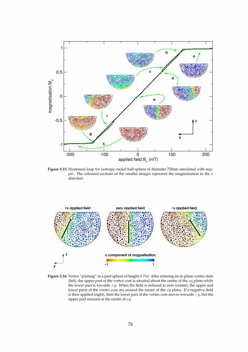
-200 -100 0 100 200applied field B

x (mT)

-1

-0.5

0

0.5

1m

agnetisation M

x

ab

c

d

e

f

g

h

y

z

Figure 5.15: Hysteresis loop for isotropic nickel half-sphere of diameter 750nm simulated with mag-par. The coloured sections of the smaller images represent the magnetisation in the xdirection

x component of magnetisation

−1 1

+x applied field zero applied field −x applied field

z

y

Figure 5.16: Vortex “pinning” in a part-sphere of height 0.75d. After entering an in-plane vortex state(left), the upper part of the vortex core is situated about the centre of the xy plane whilethe lower part is towards +y. When the field is reduced to zero (centre), the upper andlower parts of the vortex core are around the centre of the xy plane. If a negative fieldis then applied (right), then the lower part of the vortex core moves towards −y, but theupper part remains at the centre of xy.

76

-100 -50 0 50 100

applied field Bx (mT)

-1

-0.5

0

0.5

1

no

rma

lise

d m

ag

ne

tisa

tio

n M

x

A

C

D

B

Figure 5.17: The hysteresis loop for the 140nm droplet with inset x-y cut-planes showing vortex prop-agation

where lz(s) is the part which follows the outline of some bounding sphere of diam-

eter d, and lz(e) is the upper ellipsoidal dome part. These parameters most closely

reflect the geometry of droplets resulting from the partial filling of templates with

spherical voids. We study the results of simulations performed on such nanodots

with d between 50nm and 500nm.

5.5.2 Reversal mechanism

Figure 5.17 shows the hysteresis loop for a droplet with bounding sphere diameter

d = 140nm. From an initially homogeneous magnetisation brought about through

the application of a saturating magnetic field in the x direction, a slight tapering

effect appears at the surface as this field is reduced owing to long-range dipolar

interactions (see figure 5.17, point A).

Further reduction of the applied field causes the dipolar energy to become more

dominant. At slightly above zero field this causes the formation of a vortex slightly

away from the sample centre (see figure 5.17, point B), the direction of which allows

the overall magnetisation direction to remain in that of the applied field. The vortex

moves closer to the centre of the sample as the field tends towards zero, and when

there is no applied field, the Zeeman energy term is also zero and the vortex moves

77

-400 -200 0 200 400Applied field B

x (mT)

Magnetisation

140nm350nm500nm

-100 -50 0 50 100

-1

0

1

Figure 5.18: Hysteresis loops for droplets of bounding sphere diameter 140nm, 350nm and 500nm;note that the loops are offset in the y direction for clarity. Inset is the hysteresis loop fora droplet of bounding sphere diameter 50nm.

78

100 200 300 400 500Droplet bounding sphere diameter (nm)

0

5

10

15

20

25

Coerc

ive fie

ld B

c (

mT

)

Figure 5.19: Size dependence of coercive field in droplet nanodots. An error of ±1mT is present asthis is the applied field step size. Where Bc > 0mT, the remanent state is single domain,where Bc = 0mT there is a vortex remanent state.

to the centre.

The net magnetisation Mx of the sample at this point is now zero (see figure 5.17,

point C). Reducing the field further (i.e. increased in the opposite direction) shifts

the vortex further across the sample (see figure 5.17, point D), until the Zeeman

energy term influences the magnetisation more than the other energy terms and the

magnetisation of the sample becomes homogeneous in the direction of the applied

field.

It is interesting to note that if the height lz(s) from equation 5.1 is increased to

around 0.5d, the reversal mechanism is slightly different. Although the magneti-

sation falls into the vortex state, only the lower half of the vortex moves through

the system; the upper half is ‘pinned’ to the centre of the ellipsoidal part during the

entire reversal in a similar fashion to the three-quarter sphere in figure 5.16. This

gives the vortex a pendulum-like movement throughout the system. Indeed, im-

mediately after nucleation, the vortex is almost flat across the droplet in the plane

of the applied field in a similar way to the sphere in section 3.5.

79

-200 -100 0 100 200applied field B

x (mT)

-1

-0.5

0

0.5

1

ma

gn

etisa

tio

n M

x

-200 -100 0 100 200applied field B

x (mT)

-1

-0.5

0

0.5

1

ma

gn

etisa

tio

n M

x

Figure 5.20: Two hysteresis curves for nickel nanodots with bounding sphere diameter of 500nm. Thehysteresis loop on the left shows results obtained from experiment. The right-hand loopshows the results of the numerical modelling.

5.5.3 Size dependence

We have varied the diameter d of the droplet from 50nm to 500nm and computed

a hysteresis loop for every d in steps of 10nm. We find two different regimes. Fig-

ure 5.19 reflects the size dependence of the coercive field for these droplets.

When d < 140nm, the magnetisation reversal mechanism is single-domain (see

figure 5.21, left and centre). When d ≥ 140nm, the magnetisation reverses through

the vortex state (see figure 5.17 and figure 5.21, right).

The relatively consistent coercivity of 5mT between 60nm and 130nm in fig-

ure 5.19 is a result of a coherent rotation reversal process, unlike that shown by

dots smaller than 60nm. The hysteresis loops at 60nm ≤ d ≤ 130nm are substan-

tially less “square” than those shown with sub-60nm bounding sphere sizes and

bear a resemblance to the loops from 140nm and greater droplets, as indicated by

the centre loop (d=90nm)in figure 5.21.

Above 140nm the coercivity of the droplets is zero. For droplets of greater size

the hysteresis characteristics are similar, although as the size is increased the rever-

sal takes place over an increasingly large applied field, and the smaller loops at the

top and bottom of the hysteresis graph become more rounded (see figure 5.18).

There is a good agreement between the experimental hysteresis curve measured

across a nickel nanodot of bounding sphere diameter 500nm (figure 5.20, left) and

the results of the numerical simulation for the droplet of the same bounding sphere

diameter (figure 5.20, right).

5.6 Applying an out-of-plane external field

By adjusting the direction of the applied field such that it is now along the short

axis of the droplet, or out-of-plane, rather than across the symmetry plane we can

perform further studies on the droplet nanodot.

80

-200 0 200Applied field B

x (mT)

-1

0

1

No

rma

lise

d m

ag

ne

tisa

tio

n M

x


x (mT)


x (mT)

Figure 5.21: Hysteresis loops for droplet nanodots of (from left to right) bounding sphere diameter dof 30nm, 90nm and 140nm

Figure 5.22 demonstrates a typical hysteresis loop obtained from these simula-

tions and also the associated reversal mechanism. The vignette images along the

hysteresis loop show a cut-plane of the magnetisation in the xz plane, z being the

short axis and that of the applied field. Initially, a high external magnetic field is

applied such that the magnetisation becomes homogeneous in +z (point A), then

this field is gradually lowered until it is sufficiently high in the opposite direction

(−z) to maintain a homogeneous magnetisation in this direction.

As the field is reduced, the system falls into the out-of-plane vortex state with

no apparent energy barrier to overcome (point B), with the core pointing in the di-

rection of the initial applied field (point C). Further reduction of the applied field

results in the magnetisation surrounding the core pointing more towards the di-

rection of the applied field, so that when the applied field is < 0mT the overall

magnetisation is in −z (point D). The core, however, remains pointing in +z until

around −50mT, at which point the core flips causing the small jump in magnetisa-

tion around this point (point E).

Finally, once the magnetisation is sufficiently large in −z, the vortex disappears

completely and the magnetisation is homogeneous in −z (point F).

Figure 5.23 shows the size dependence of the droplets when the applied field

is out of the plane. The coercive field of the droplets decreases as the bounding

sphere radius is increased, with the rate of coercivity reduction decreasing as the

radius is further increased.

Figure 5.24 places the coercive field size dependence of the droplets where the

initial applied field is out of the plane into context by comparing this to the coer-

civity of the same droplets when the original applied field is in the plane. It is clear

from these results that applying the field across the short out-of-plane axis of the

droplets increases the coercivity significantly; for a coercive field of 20mT a droplet

of bounding sphere diameter of around 25nm is sufficient with an in-plane applied

field, however with an out-of-plane field a bounding sphere diameter of ≈160nm

is required.

81

-400 -200 0 200 400applied field B

z (mT)

-1

-0.5

0

0.5

1

ma

gn

etisa

tio

n M

z

AB

C

D

E

F

Figure 5.22: Reversal mechanism of a nickel droplet of bounding sphere diameter 200nm in a per-pendicular applied field

82

50 60 70 80 90 100bounding sphere radius (nm)

10

20

30

40

50

coerc

ivity B

c (

mT

)

100 120 140 160 180 200

bounding sphere diameter (nm)

Figure 5.23: Size dependence of the out-of-plane coercive field in droplet nanodots.

83

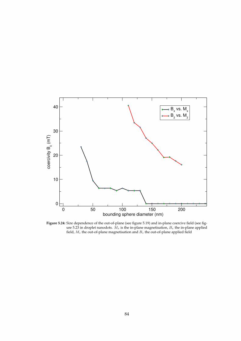
0 50 100 150 200bounding sphere diameter (nm)

0

10

20

30

40

coerc

ivity B

c (

mT

)

Bx vs. M

x

Bz vs. M

z

Figure 5.24: Size dependence of the out-of-plane (see figure 5.19) and in-plane coercive field (see fig-ure 5.23 in droplet nanodots. Mx is the in-plane magnetisation, Bx the in-plane appliedfield, Mz the out-of-plane magnetisation and Bz the out-of-plane applied field

84

5.7 Summary

We have simulated the magnetisation reversal in part-spherical and droplet nan-

odots. In droplet nanodots, we observe two different mechanisms for this reversal

— the single-domain state and the vortex state.

If the overall size of the droplet system is increased then we notice a distinct

transition from the single domain state to the vortex state, which we identify for

isotropic nickel (see appendix C) as being at a droplet bounding sphere diameter of

140nm (physical droplet diameter in this instance is around 90% of the bounding

sphere diameter, approximately 126nm, and h =3/7d = 60nm). This change occurs

at a smaller diameter than for thin (h ≤ 30nm) circular nanodots (see figure 3.10).

The “soft” vortex behaviour — i.e. the vortex will readily adjust its position to

accommodate a change in applied field — observed in the large droplets is a useful

characteristic in sensor applications; smaller droplets have the square hysteresis

loops desirable for data storage.

In part-spherical particles, three separate remanent states — single-domain,

out-of-plane vortex and in-plane vortex — have been observed.

As the diameter of the part-spherical particle decreases, a larger h/d is necessary

for a vortex to form. As h is increased, the magnetisation is more likely to form a

vortex. Below a critical radius of 12.4nm for Ni50Fe50, all h/d values will result in a

single-domain remanent state.

The hysteresis loops observed experimentally agree well with the numerical

results from the simulation.

We observe good agreement between the finite difference method in OOMMF

and the hybrid finite element/boundary element model in magpar.

85

Chapter 6

Antidots

Parts of this work have been submitted for publication as Zhukov et al. (2004a)

and Zhukov et al. (2004b). Experimental measurements were obtained by Dr. Alexan-

der Zhukov of the School of Physics and Astronomy (University of Southampton)

and the Monte Carlo simulations performed by Dr. Hans Fangohr of the School of

Engineering Sciences (University of Southampton).

6.1 Introduction

Lithographic techniques have allowed researchers to create ordered structures on

the sub-micron scale (Cowburn et al., 1997, Fruchart et al., 1999, Hehn et al., 1996,

Martın et al., 2003, Van Roy et al., 1993), either as well-formed small magnetic ele-

ments such as the cylindrical and spherical objects described in chapters 3 and 5

or as regular arrays of holes in magnetic films. Antidots are the ‘opposite’ of the

nanodots discussed in the previous chapter. If one creates a hole in a thin sam-

ple, the hole can be considered to be an antidot. Lithographic techniques generally

yield cylindrical holes, but emerging self-assembly techniques (Bartlett et al., 2002)

promise a wider range of shapes.

Figure 6.1 shows the single-template self-assembly technique. Electrochemical

deposition can be used to create nanoscale magnetic materials by creating an or-

dered template from polystyrene latex spheres of size order 50nm ≤ d ≤ 1000nm

(Bartlett et al., 2003b, Xu et al., 2000). Initially, an aqueous solution of monodisperse

latex spheres is deposited on a glass substrate. On this substrate sputtered buffer

layers of chromium and gold have been deposited, with thicknesses of 10nm and

200nm respectively.

Over a period of between three and five days the evaporation of the water leads

to the formation of the template: the combination of the electrostatic repulsion be-

tween the latex spheres and the attractive capillary forces provided by the evapo-

ration of the water produces a well-ordered close-packed structure (Bartlett et al.,

2002, 2000, 2003b).

86

h

d

water latex spheres

substrate

magnetic material

Figure 6.1: The single-template self-assembly technique. Latex spheres of diameter d are poured onto a substrate (left). As the water evaporates, the latex spheres become close-packed,forming a template (centre) which can then be filled with a magnetic material from thesubstrate upwards to a height h (right).

Using electrodeposition from the gold layer, the electrodeposited material fills

the spaces between the latex spheres, using the spheres as a mould. By dissolving

the latex spheres in toluene, 3D antidot arrays with spherical holes are formed.

Different thicknesses of antidot arrays can be formed by adjusting the charge

during the electrodeposition process, while the period of the antidots is controlled

by altering the diameter of the latex spheres.

Figure 6.2 shows a scanning electron microscope image of an antidot array cre-

ated through the self-assembly template method, and demonstrates the regular

structure formed with this process.

Figure 6.3 shows the experimentally-measured coercivity of Ni50Fe50 antidot

arrays with a diameter d of 550nm when the external field is applied in-plane. The

coercivity oscillates as a function of height (thickness) h. When the height of the

film is close to the sphere centres, the coercivity reaches a local maximum. This

oscillatory behaviour is what we wish to understand and explain in this chapter.

6.1.1 The hexagonal lattice

For a hexagonal lattice with base vectors:

a1 = ax (6.1)

a2 =1

2ax+

√3

2ay (6.2)

a3 =

√

8

3az (6.3)

the lattice points are:

P = n1a1 + n2a2 + n3a3 (6.4)

(n1, n2, n3) ∈ N3 (6.5)

87

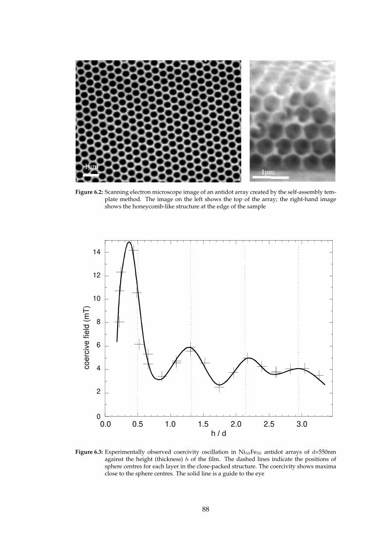
Figure 6.2: Scanning electron microscope image of an antidot array created by the self-assembly tem-plate method. The image on the left shows the top of the array; the right-hand imageshows the honeycomb-like structure at the edge of the sample

co

erc

ive

fie

ld (

mT

)

0

10

2

4

6

8

12

14

1.0 2.0 2.5 3.00.0 0.5 1.5

h / d

Figure 6.3: Experimentally observed coercivity oscillation in Ni50Fe50 antidot arrays of d=550nmagainst the height (thickness) h of the film. The dashed lines indicate the positions ofsphere centres for each layer in the close-packed structure. The coercivity shows maximaclose to the sphere centres. The solid line is a guide to the eye

88

Figure 6.4: Two layers of spheres packed cubically (left) and hexagonally (right)

Shown in figure 6.4 on the right is a hexagonal structure which exhibits this prop-

erty. However, one should note that there are two ways of packing this layer as

there are two positions in which the first sphere can be placed. The two structures

are called hexagonal close-packed and face-centred cubic. The hexagonal close-packed

structure, or hcp, has the third layer in c having the same x and y coordinates as

the first layer, the second layer has the same x and y coordinates as the fourth layer

(ABABAB. . . ) and so on (Kittel, 1996). The face-centred cubic structure has an alter-

native arrangement of spheres in the third layer where the spheres share the same

x coordinate with the first layer but have different y coordinates (ABCABC. . . ).

Although this arrangement appears at the outset to be hexagonal, by rotating its

primitive cell the vectors can be shown to be a variant of a cubic lattice.

6.2 Parameters of the antidot system

Since three-dimensional arrays of objects become rapidly impractical to simulate

even across modern supercomputing clusters, a feasibility study was conducted to

assess the limits of the available hardware when computing the hysteresis loops for

these systems.

A set of different self-assembled experimental samples were prepared from

nickel, iron, cobalt and Ni50Fe50 permalloy from spheres sized 20nm ≤ d ≤ 1000nm.

For the initial micromagnetic study we chose to model the nickel sample. Nickel

has a relatively large exchange length (λex ≈ 7.5nm) when compared to Ni50Fe50

permalloy (λex ≈ 2.75nm), allowing for physically larger systems to be computed

within a simulation domain of a comparable discrete cell count.

For the simulations, the parameters for amorphous nickel were selected (Ms =

4.93×105 A/m, A = 8.5×10−12 J/m, K1 = 0 J/m3) and to improve convergence a

damping constant α of 0.25 was chosen.

89

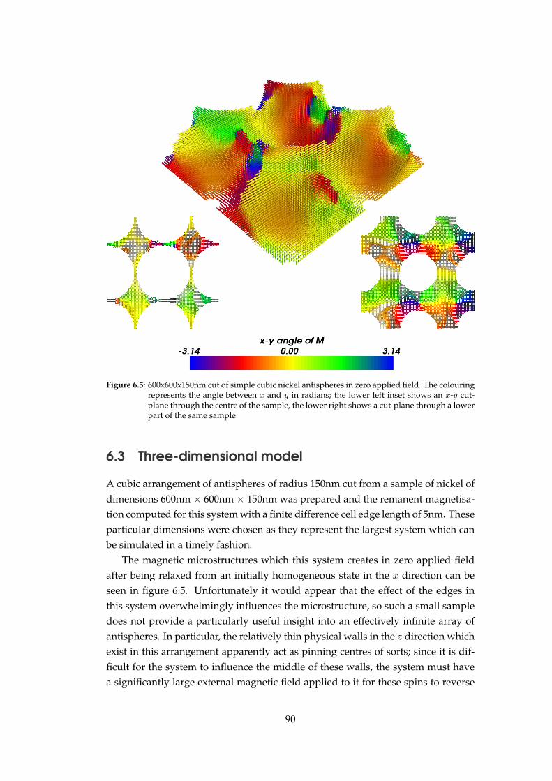
Figure 6.5: 600x600x150nm cut of simple cubic nickel antispheres in zero applied field. The colouringrepresents the angle between x and y in radians; the lower left inset shows an x-y cut-plane through the centre of the sample, the lower right shows a cut-plane through a lowerpart of the same sample

6.3 Three-dimensional model

A cubic arrangement of antispheres of radius 150nm cut from a sample of nickel of

dimensions 600nm × 600nm × 150nm was prepared and the remanent magnetisa-

tion computed for this system with a finite difference cell edge length of 5nm. These

particular dimensions were chosen as they represent the largest system which can

be simulated in a timely fashion.

The magnetic microstructures which this system creates in zero applied field

after being relaxed from an initially homogeneous state in the x direction can be

seen in figure 6.5. Unfortunately it would appear that the effect of the edges in

this system overwhelmingly influences the microstructure, so such a small sample

does not provide a particularly useful insight into an effectively infinite array of

antispheres. In particular, the relatively thin physical walls in the z direction which

exist in this arrangement apparently act as pinning centres of sorts; since it is dif-

ficult for the system to influence the middle of these walls, the system must have

a significantly large external magnetic field applied to it for these spins to reverse

90

Figure 6.6: Magnetisation of a cobalt hexagonal antidot array in zero field; direction of initial appliedfield θ = 30o, d = 300nm, r

R= 0.4, h = 0.05d

their direction of magnetisation.

For more useful results to be obtained, a much larger system is required. Instead

of 3 × 3 antisphere centres being present in the system, we estimate 5 × 5 or more

centres would be necessary to reduce the effects of the sample edges enough to

accurately reflect the microstructures which form within the experimental sample.

Zhukov et al. (2003) perform experimental measurements on large hexagonal ar-

rays of isotropic Ni50Fe50 permalloy antispheres (Ms = 1.1×106 A/m, A = 5.85×10−12

J/m, K1 = 0 J/m3); this permalloy variant has a particularly small exchange length

(λex = 2.76 nm) and as such requires a finer mesh. When this fine mesh is combined

with the need for a large number of antisphere centres, it becomes unrealistic to

perform even one simulation of the resulting structure.

6.4 Two-dimensional model

By considering only two-dimensional cut-planes of the hexagonal antispheres —

assuming that the individual layers behave independently — it is possible to simu-

late significantly larger systems in the x and y directions than if attempting to per-

form a simulation across a three-dimensional sample of similar proportions. We

can then measure the coercive field for different layers.

The hexagonal antisphere systems in Zhukov et al. (2003) can be mapped to

two-dimensional samples by considering hexagonally-spaced circular holes — flat

91

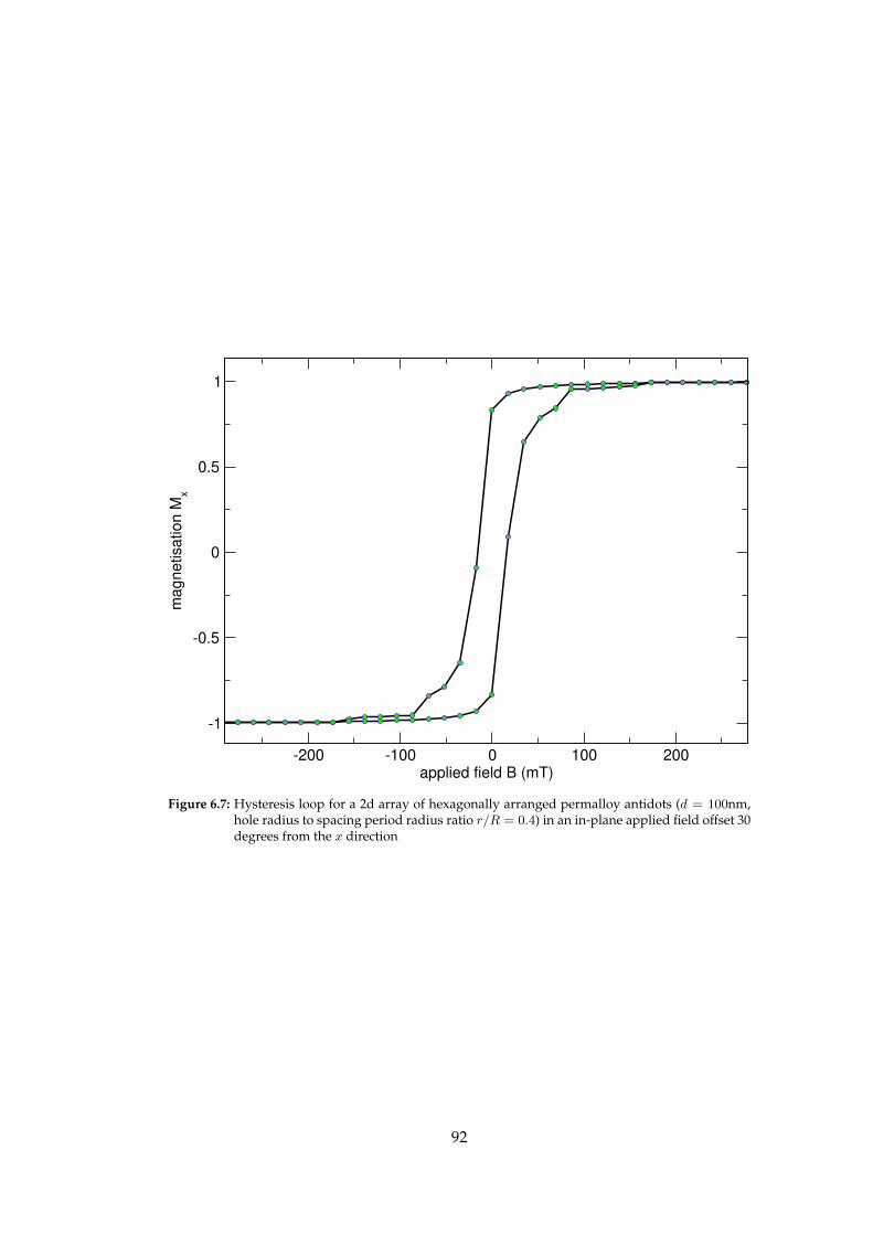
-200 -100 0 100 200applied field B (mT)

-1

-0.5

0

0.5

1

ma

gn

etisa

tio

n M

x

Figure 6.7: Hysteresis loop for a 2d array of hexagonally arranged permalloy antidots (d = 100nm,hole radius to spacing period radius ratio r/R = 0.4) in an in-plane applied field offset 30degrees from the x direction

92

antidots — in a thin film. By varying the ratio of hole radius r to spacing radius R

the surface of the antisphere geometry at different heights can be modelled reason-

ably accurately. Since larger systems can be simulated, the influence of the sample

edges detailed in section 6.3 is substantially reduced (figure 6.6).

6.5 Stray field measurement

The development of the scanning tunnelling microscope (STM) allowed scientists

to determine the electronic topography of a sample with a resolution down to a

few angstroms (Binnig and Rohrer, 1985, Binnig et al., 1982, 1983). The atomic force

microscope (AFM) is a further development of the STM which exploits the defor-

mation of a spring attached to a cantilever to allow the measurement of the force

exerted on the sharp AFM tip (Binnig et al., 1986).

To characterise the magnetic properties of a sample, the standard diamond tip

of the AFM is replaced by a ferromagnetic tip (Rugar et al., 1990, Saenz et al., 1987)

allowing the observation of magnetic domain structures by measuring the force

gradient exerted on the tip by the stray field as a function of the position — a tech-

nique known as magnetic force microscopy (MFM) . Rather than the tip following

the surface contours of the sample as in STM, the MFM operates with the tip at a

fixed z point in space.

To assess the appropriateness of the two-dimensional approximation above, we

compute the stray field and compare this to the experimental images provided

through magnetic force microscopy.

The tip of an MFM is magnetic and we assume that it is a dipole d. In the

absence of knowledge of the precise magnetisation of the tip, this is the simplest

approach possible (Barthelmeß et al., 2003). The signal which the MFM records is

proportional to the gradient of the demagnetising field Hde.

6.5.1 Numerical calculation of the stray field

We compute the stray field from our simulation data as it would be read from a

magnetic force microscope by simulating several layers of “empty space” above

the sample and measuring the demagnetising field. This has the advantage that

the efficient OOMMF algorithm for the computation of the demagnetising field can

be used. However, we need to compute the second derivative numerically (using

central differences):

∂2f

∂x2=

f(x+ h)− 2f(x) + f(x− h)

h2+O(h2) (6.6)

93

Figure 6.8: Microscopic images of an antidot array. The tunnelling image on the left shows the lo-cation of the antidots; the magnetic force microscopy image on the right highlights thedemagnetisation field

where h is the distance between the upper and lower layers of the demagnetising

field.

6.5.2 Stray field calculation through analytical techniques

Alternatively, we can interpret the discrete magnetisation vector M(r) at the sur-

face of the sample as a layer of dipoles and compute the stray field at the MFM tip

and consequently the second derivative analytically.

This approach is more accurate in determining the second derivative because

h in equation 6.6 cannot be made arbitrarily small. Additionally, an analytical ap-

proach is more flexible with respect to the fly height of the MFM tip.

It should be noted that this approach ignores the higher order magnetic mo-

ments associated with each simulation cell in OOMMF by replacing them with the

leading dipole term. This is justified if the height of the MFM tip above the sample

surface is much greater than the OOMMF cell spacing.

The second derivative of the demagnetising energy should be proportional to

the signal at the tip of a magnetic force microscope and can be shown (see ap-

pendix A) to be:

94

Figure 6.9: Demagnetising field of an antidot sample in zero applied field as measured by the tip ofthe magnetic force microscope (left) and the second derivative as computed through theanalytical techniques from equation 6.7 (right)

∂2Ed

∂z′2= µ0

(−3 ·m ·m′

|r− r′|5

+15 ·m ·m′(z − z′)2

|r− r′|7

−6 ·m′zmz

|r− r′|7

+30(m · (r− r′))m′

z(z − z′)

|r− r′|7

+30(m′ · (r− r′))mz(z − z′)

|r− r′|7

+15(m · (r− r′))(m′ · (r− r′))

|r− r′|7

−105(m · (r− r′))(m′ · (r− r′))(z′ − z′)2

|r− r′|9)

(6.7)

This assumes that the tip of the MFM is a dipole:

m′ =

0

0

C

(6.8)

The full derivation of this can be found in appendix A.

Figure 6.9 shows the comparison between the experimental data measured with

a magnetic force microscope in zero applied field and the second derivative of the

demagnetising field as calculated by the above equation. There is a significant sim-

ilarity between the images; both show a characteristic periodic parallelogram pat-

tern. The tip distance, both experimental and computed, was half of the distance

between the antidot centres.

Figure 6.10 shows a clear agreement between the measurements from the MFM

95

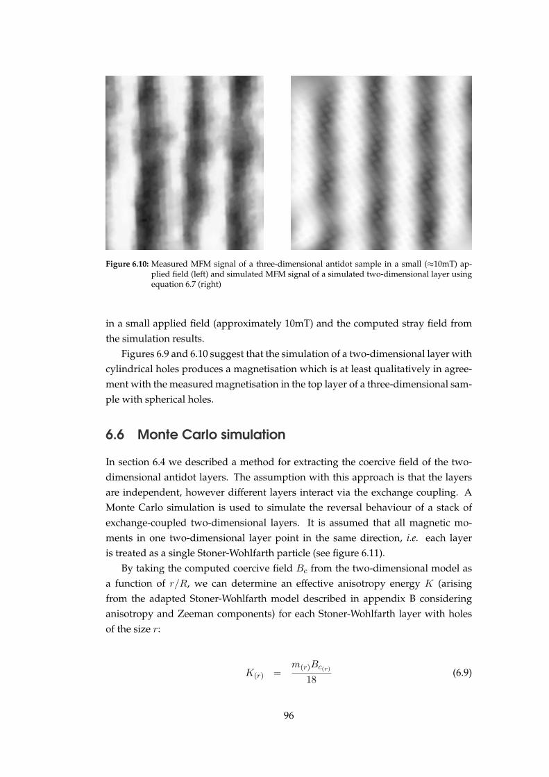
Figure 6.10: Measured MFM signal of a three-dimensional antidot sample in a small (≈10mT) ap-plied field (left) and simulated MFM signal of a simulated two-dimensional layer usingequation 6.7 (right)

in a small applied field (approximately 10mT) and the computed stray field from

the simulation results.

Figures 6.9 and 6.10 suggest that the simulation of a two-dimensional layer with

cylindrical holes produces a magnetisation which is at least qualitatively in agree-

ment with the measured magnetisation in the top layer of a three-dimensional sam-

ple with spherical holes.

6.6 Monte Carlo simulation

In section 6.4 we described a method for extracting the coercive field of the two-

dimensional antidot layers. The assumption with this approach is that the layers

are independent, however different layers interact via the exchange coupling. A

Monte Carlo simulation is used to simulate the reversal behaviour of a stack of

exchange-coupled two-dimensional layers. It is assumed that all magnetic mo-

ments in one two-dimensional layer point in the same direction, i.e. each layer

is treated as a single Stoner-Wohlfarth particle (see figure 6.11).

By taking the computed coercive field Bc from the two-dimensional model as

a function of r/R, we can determine an effective anisotropy energy K (arising

from the adapted Stoner-Wohlfarth model described in appendix B considering

anisotropy and Zeeman components) for each Stoner-Wohlfarth layer with holes

of the size r:

K(r) =m(r)Bc(r)

18(6.9)

96

��

��

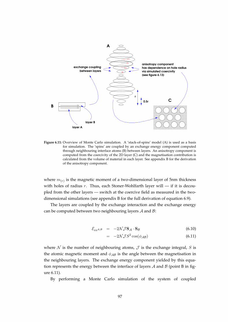
0.5r

r

between layers

exchange coupling

layer B

layer A

C

A

B

anisotropy component

has dependence on hole radius

via simulated coercivity

(see figure 6.13)

Figure 6.11: Overview of Monte Carlo simulation. A ‘stack-of-spins’ model (A) is used as a basisfor simulation. The ‘spins’ are coupled by an exchange energy component computedthrough neighbouring interface atoms (B) between layers. An anisotropy component iscomputed from the coercivity of the 2D layer (C) and the magnetisation contribution iscalculated from the volume of material in each layer. See appendix B for the derivationof the anisotropy component.

where m(r) is the magnetic moment of a two-dimensional layer of 5nm thickness

with holes of radius r. Thus, each Stoner-Wohlfarth layer will — if it is decou-

pled from the other layers — switch at the coercive field as measured in the two-

dimensional simulations (see appendix B for the full derivation of equation 6.9).

The layers are coupled by the exchange interaction and the exchange energy

can be computed between two neighbouring layers A and B:

EexA,B = −2NJSA · SB (6.10)

= −2NJ S2 cos(φAB) (6.11)

where N is the number of neighbouring atoms, J is the exchange integral, S is

the atomic magnetic moment and φAB is the angle between the magnetisation in

the neighbouring layers. The exchange energy component yielded by this equa-

tion represents the energy between the interface of layers A and B (point B in fig-

ure 6.11).

By performing a Monte Carlo simulation of the system of coupled

97

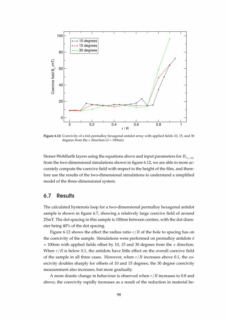
0 0.2 0.4 0.6 0.8 1r / R

0

20

40

60

80

100

Coerc

ive fie

ld B

c (

mT

)

10 degrees

15 degrees

30 degrees

Figure 6.12: Coercivity of a 6x6 permalloy hexagonal antidot array with applied fields 10, 15, and 30degrees from the x direction (d = 100nm).

Stoner-Wohlfarth layers using the equations above and input parameters for Bc(r/R)

from the two-dimensional simulations shown in figure 6.12, we are able to more ac-

curately compute the coercive field with respect to the height of the film, and there-

fore use the results of the two-dimensional simulations to understand a simplified

model of the three-dimensional system.

6.7 Results

The calculated hysteresis loop for a two-dimensional permalloy hexagonal antidot

sample is shown in figure 6.7, showing a relatively large coercive field of around

25mT. The dot spacing in this sample is 100nm between centres, with the dot diam-

eter being 40% of the dot spacing.

Figure 6.12 shows the effect the radius ratio r/R of the hole to spacing has on

the coercivity of the sample. Simulations were performed on permalloy antidots d

= 100nm with applied fields offset by 10, 15 and 30 degrees from the x direction.

When r/R is below 0.1, the antidots have little effect on the overall coercive field

of the sample in all three cases. However, when r/R increases above 0.1, the co-

ercivity doubles sharply for offsets of 10 and 15 degrees; the 30 degree coercivity

measurement also increases, but more gradually.

A more drastic change in behaviour is observed when r/R increases to 0.8 and

above; the coercivity rapidly increases as a result of the reduction in material be-

98

0 0.2 0.4 0.6 0.8 1r/R

0

5

10

15

20

25

30

coerc

ive fie

ld B

c (

mT

)

Figure 6.13: Coercivity of a larger 6x6 permalloy hexagonal antidot array with the applied field offset30 degrees from the x axis (d = 200nm).

tween the antidots; this makes it more difficult for the system to reverse the mag-

netisation between these thin ‘walls’ of material. In the most extreme case, the co-

ercivity of the 30 degree sample when r/R is 0.9 is approximately ten times greater

than that when r/R is 0.1 and below.

Any simulation performed in the situation where r/R is 1.0 is likely to be in-

accurate as the finite resolution of the simulation will not allow the extremely fine

walls around the point where the antidots touch to be precisely resolved.

Figure 6.13 shows a coercive field graph of a 30o offset permalloy antidot sys-

tem, similar to that shown in figure 6.12 only with d = 200nm. In this larger system,

the jump in the system at r/R = 0.1 is less pronounced and the coercivity increases

in a less abrupt fashion.

Figure 6.14 shows the results of the Monte Carlo simulation using values of Bc(r)

from the d = 200nm permalloy dataset demonstrated in figure 6.13, comparable to

the experimental results shown in figure 6.3.

Figure 6.15 shows on the left an experimental magnetic force microscope im-

age of a cobalt antidot film (d = 700nm, h = 100nm) in zero applied field. The

holes at the surface of the antidot film are indicated by the blue circles. The image

on the right-hand side shows the remanent magnetisation pattern from the two-

99

10

15

coerc

ive fie

ld (

mT

)

h / d0.0 0.5 1.0 1.5 2.0 2.5 3.0 3.5

Figure 6.14: Monte Carlo simulation results with Bc(r/R)values from figure 6.13

dimensional micromagnetic modelling case when r/R = 0.5. In both cases the

applied field was 30 degrees from the indicated x axis.

The numerical results show that the magnetisation follows around the holes,

forming a consistent periodic microstructure. The magnetisation between neigh-

bours in a1 (see equation 6.1) is 90 degrees from x (60 degrees from the applied

field), but between neighbours in a2 the magnetisation is 60 degrees from x (30 de-

grees from the applied field). The magnetisation between neighbours in

(−a2(x),a2(y)) is 30 degrees from x (aligned with the applied field).

6.8 Summary

We have calculated hysteresis loops, magnetisation patterns and stray fields over

antidot samples, and whilst three-dimensional micromagnetic simulations will al-

ways be the most accurate way of simulating these shapes, it is not always practical.

In certain situations, particularly where a large simulation domain is desir-

able, a two-dimensional simulation which accurately reflects the three-dimensional

physical sample can offer insight into the magnetisation patterns and in particular

the stray field patterns in these physical samples.

In addition, the strong similarity between the experimental MFM results and

the computed stray field from the simulation allows us to conclude that the two-

dimensional model is a reasonably accurate reflection of the three-dimensional ex-

perimental system.

100

y

x

Figure 6.15: Experimental and numerical images for a cobalt antidot film (left) MFM image of filmprepared with spheres of diameter 700nm with thickness 100nm; blue circles indicatethe position of the holes in the film and (right) magnetisation direction from numericalmodelling with r/R = 0.5; the colour scale represents the magnetisation angle in the xyplane in radians

6.8.1 Outlook

By using periodic boundary conditions, unfortunately not available in the

simulation software, it would be possible to compute a system in three dimen-

sions by making the sample periodic in the x and y directions. Parallel execution

of the simulation code coupled with a shared memory model would also make the

three-dimensional simulation case feasible.

The next steps in following up the presented results would be to further un-

derstand the three regimes in Bc(r/R) for two-dimensional systems shown in fig-

ure 6.12, in addition to modelling the full three-dimensional system.

101

Chapter 7

Summary and outlook

7.1 Summary

We have investigated the properties of micromagnetic samples through simulation

paying particular attention to shape anisotropy — the influence the shape has on

the hysteresis loop and magnetic microstructure.

Most magnetic samples at a nanometre scale possess characteristics desirable

for magnetic data storage applications, either as data read/write heads or sensors,

where the magnetisation is sensitive to small changes in B, or as storage media

with a high coercivity.

We note that cylinders are particularly suitable candidates for storage media

when considering their comparatively large coercivity, and our phase diagram iden-

tifies the behavioural dependence on diameter and height. Spherical geometries

exhibit properties useful for magnetic sensors. Our studies reveal how coercivity

decreases when overall diameter is increased.

More complex shapes, such as the cone, half-sphere and the droplet are more

flexible, and by subtle alterations in their sizes can be manipulated for use in any

data storage application. Size dependence studies in the droplet geometry show

that the transition between the single-domain and the vortex state occurs at a bound-

ing sphere diameter of 140nm in nickel. Larger droplets which have reversible

characteristics and zero coercivity are ideal for magnetic sensor applications.

Antidots show interesting characteristics when considered in arrays of their

peers, and given the flexibility of the coercive field through altering the size of the

dots as a fraction of the spacing distance, make good candidates for storage media.

Comparisons between our simulations and experimental results demonstrate a

high degree of similarity. We can use micromagnetic simulation to observe hys-

teretic behaviour and coercivity trends with high confidence, and the study of sam-

ples with other geometries and sizes which are not yet feasible for experimentalists

to physically produce can yield possible directions for future experimental work.

Overall, we conclude the coercivity of magnetic samples can be controlled by

102

their physical shape and size.

Possible candidates for further simulation include the remainder of the prim-

itive set — torii and pyramids — as well as constructive solid geometries based

upon these primitives, for example a tear-drop shape built from a conical upper

and a half-ellipsoid lower section. Shapes such as these could be created by com-

bining the self-assembly double-template method outlined in chapter 5 with elec-

tron beam lithographic techniques. Using this method it is also possible to create

films manufactured from different materials — for example, it might be possible to

create a cobalt half-sphere which has a permalloy “hat”.

The simulations presented in this thesis were computed as zero temperature.

Thermal effects, even at low temperatures, can introduce subtle changes in be-

haviour. As such, the contribution to the results through finite temperature would

be studied in a continuation of this work. Initial studies indicate that the size of

secondary hysteresis loop energy barriers in the case of the sphere is reduced at

finite temperature.

The work discussed in section 5.5.2 revealed some interesting properties of

vortex behaviour in the droplets. Initial studies have shown that the droplets,

especially larger ones, demonstrate similar vortex orientations to those found in

spheres, although they quickly fall into a more disc-like out-of-plane vortex state

as the applied field is further reduced.

A more detailed study will be performed into how the variation of lz(s) and lz(e)

from equations 5.1 and 5.1 affects the vortex formation, movement and subsequent

disappearance. The effect of magnetostatic energy between adjacent nanodots will

also be investigated.

Finally, in chapter 6 we compared experimental data with simulation results

produced through two-dimensional simulations, Monte Carlo methods and found

a strong similarity between experimental MFM and computed stray field results,

corroborating the two-dimensional model presented in that chapter.

103

Appendix A

Analytical calculation of the

stray field

Since the phase shift of the cantilever attached to the sharp tip in a magnetic force

microscope (Saenz et al., 1987) when measured corresponds to the measured sig-

nal (McVitie et al., 2001), the second derivative of the stray field (Hug et al., 1998, Ru-

gar et al., 1990) is proportional to the rate of change of the force on the tip (Barthelmeß

et al., 2004).

If the second derivative is evaluated at a fixed height above a demagnetising

energy dataset of micromagnetic simulation results then this is comparable to a

magnetic force microscope. This derivative is presented in this appendix.

The dipolar energy between two points in a magnetic system, assuming each

discrete cell is a dipole, can be considered to be

Epot = µ0m ·m′ − 3(m · e)(m′ · e)

|r− r′|3 ∀r 6= r′ (A.1)

where e is the unit vector of r.

For fixed m′ (such as that in the magnetic tip in magnetic force microscopy), the

effective field is

Hd =m− 3(m · e)e

|r− r′|3 (A.2)

because E = −µ0m ·Hd, noting that m is located at r and m′ — the tip — is located

at r′. We define:

e =r− r′

|r− r′| (A.3)

For the MFM data:

∂2Epot

∂z′2∝ ∂2Hz

d

∂z′2(A.4)

104

Expand A.1 by substituting A.3:

Epot = µ0m ·m′

|r− r′|3 − 3(m · (r− r′)) · (m′ · (r− r′))

|r− r′|5 (A.5)

We precompute some expressions:

g(r, r′) ≡ |r− r′| (A.6)

=√

(x− x′)2 + (y − y′)2 + (z − z′)2 (A.7)(

=√

(r− r′)2)

(A.8)

∂g(r, r′)

∂z′=

1

2√

(r− r′)2· 2(−1)(z − z′) (A.9)

=1

√

(r− r′)2· −1(z − z′) (A.10)

=−(z − z′)

|r− r′| (A.11)

=z′ − z

|r− r′| (A.12)

f ≡ g3 (A.13)

= |r− r′|3 (A.14)

∂f

∂z′=

∂f

∂g· ∂g∂z′

(A.15)

= 3 · g(r, r′)2 · ∂g∂z′

(r, r′) (A.16)

= 3|r− r′|2 · z′ − z

|r− r′| (A.17)

= 3|r− r′|(z′ − z) (A.18)

f ≡ 1

f(A.19)

=1

g3(A.20)

=1

|r− r′|3 (A.21)

= g−3 (A.22)

105

∂f

∂z′=

∂f

∂g

∂g

∂z′(A.23)

= −3g−4 · ∂g∂z′

(A.24)

= −31

|r− r′|4 · z′ − z

|r− r′| (A.25)

= −3z′ − z

|r− r′|5 (A.26)

h ≡ g5 (A.27)

so

∂h

∂z′=

∂h

∂g

∂g

∂z′(A.28)

= 5g4 · z′ − z

|r− r′| (A.29)

= 5|r− r′|3 · (z′ − z) (A.30)

h ≡ g−5 (A.31)

so

∂h

∂z′=

∂h

∂g

∂g

∂z′(A.32)

= −5g−6 z′ − z

|r− r′| (A.33)

= −5z′ − z

|r− r′|7 (A.34)

Looking at the mixed terms in A.5:

Ψ(r, r′) ≡[

m · (r− r′)][

m′ · (r− r′)]

(A.35)

=[

mx(x− x′) +my(y − y′) +mz(z − z′)]

·[

m′x(x− x′) +m′

y(y − y′) +m′z(z − z′)

]

(A.36)

∂Ψ

∂z′=

[

m(r− r′)]

· ∂

∂z′(

m′x(x− x′) +m′

y(y − y′) +m′z(z − z′)

)

+[

m′(r− r′)]

· ∂

∂z′(

mx(x− x′) +my(y − y′) +mz(z − z′))

= m(r− r′) · (−m′z) +m′(r− r′) · (−mz) (A.37)

106

φ ≡ Ψ

|r− r′|5 (A.38)

=Ψ

h(A.39)

∂φ

∂z′=

h · ∂Ψ∂z′ −Ψ · ∂h

∂z′

h2(A.40)

=g5 · ∂Ψ

∂z′ −Ψ · 5g3(z′ − z)

g10(A.41)

=∂Ψ∂z′

g5− 5Ψ(z′ − z)

g7(A.42)

=−m · (r− r′) ·m′

z −m′ · (r− r′)mz

|r− r′|5

−5(m · (r− r′))(m′(r− r′))(z′ − z)

|r− r′|7 (A.43)

Combining the above to give the first derivative of the dipolar interaction energy

as A.5:

Epot = µ0

( m ·m′

|r− r′|3 − 3(m · (r− r′))(m′ · (r− r′))

|r− r′|5)

(A.44)

With respect to z′:

∂Epot

∂z′= µ0

(

m ·m′ · 3(z − z′)

|r− r′|5

+3m · (r− r′) ·m′

z + 3m′(r− r′)mz

|r− r′|5

+35(m · (r− r′))(m′ · (r− r′))(z′ − z)

|r− r′|7)

(A.45)

= µ0(A+D + E + F) (A.46)

A ≡ 3m ·m′(z − z′)

|r− r′|5 (A.47)

D ≡ 3m(r− r′) ·m′z

|r− r′|5 (A.48)

E ≡ 3m′(r− r′) ·mz

|r− r′|5 (A.49)

F ≡ 15(m · (r− r′))(m′ · (r− r′))(z′ − z)

|r− r′|7 (A.50)

107

A =BC (A.51)

To find∂2Epot

∂z′2, we need the derivatives of A, D, E and F :

∂A∂z′

=C · ∂B

∂z′ − B · ∂C∂z′

C2(A.52)

=|r− r′|5 · 3m ·m′(−1)− 3m ·m′(z − z′) · 5|r− r′|3(z′ − z)

|r− r′|10 (A.53)

=−3m ·m′

|r− r′|5 +15m ·m′(z − z′)2

|r− r′|7 (A.54)

∂D∂z′

=C · ∂

∂z′ (3m · (r− r′) ·m′z)− 3m(r− r′) ·m′

z · 5|r− r′|3(z′ − z)

|r− r′|10 (A.55)

=3m′

z∂∂z′ (mx(x− x′) +my(y − y′) +mz(z − z′))

|r− r′|5

+15m(r− r′)m′

z(z − z′)

|r− r′|7 (A.56)

=3m′

z(−mz)

|r− r′|5 +15m′

z(z − z′)(r− r′) ·m|r− r′|7 (A.57)

∂E∂z′

=3|r− r′|5 ∂

∂z′ (m′x(x− x′) +m′

y(y − y′) +m′z(z − z′)) ·mz

|r− r′|10

−3m′(r− r′) ·mz · 5|r− r′|3(z′ − z)

|r− r′|10 (A.58)

=3(−m′

zmz)

|r− r′|5 +15m′(r− r′)mz(z − z′)

|r− r′|7 (A.59)

r0 = 15(m · (r− r′)) · (m′ · (r− r′)) (A.60)

= 15(mx(x− x′) +my(y − y′) +mz(z − z′))

·(m′x(x− x′) +m′

y(y − y′) +mz(z − z′)) (A.61)

F1 = r0(z′ − z) (A.62)

In the derivative, only the terms with z′ matter:

F0 =F1

z′ − z(A.63)

108

∂F0

∂z′=

∂

∂z′(

15(

mx(x− x′)m′z(z − z′)

+my(y − y′)m′z(z − z′)

+mz(z − z′)m′z(z − z′)

))

(A.64)

∂

∂z′= mzm

′z · 2(z − z′)(−1) (A.65)

∂F0

∂z′= 15(mx(x− x′)m′

z(−1)

+my(y − y′)m′z(−1)

+mzm′z · 2(z − z′)(−1)

+mzm′x(x− x′)(−1)

+mzm′y(y − y′)(−1))

= −15(m · (r− r′) ·m′z +m′ · (r− r′) ·mz) (A.66)

∂F1

∂z′= F0

∂

∂z′(z′ − z) + (z′ − z)

∂F0

∂z′(A.67)

= 15(m · (r− r′))(m′ · (r− r′)) · 1+(z′ − z)(−15)(m · (r− r′)m′

z +m′(r− r′)mz) (A.68)

= 15((m · (r− r′))

+m · (r− r′)m′z(z − z′)

+m′ · (r− r′)mz(z − z′)) (A.69)

q ≡ g7 (A.70)

= |r− r′|7 (A.71)

∂q

∂z′=

∂q

∂g

∂g

∂z′(A.72)

= 7g6∂g

∂z′(A.73)

=7g6(z′ − z)

g(A.74)

= 7|r− r′|5(z′ − z) (A.75)

109

∂F∂z′

=g7 · ∂F1

∂z′ −F1 · ∂g7

∂z′

(g7)2(A.76)

=∂F1∂z′

g7− F1 · ∂g7

∂z′

g14(A.77)

=15

|r− r′|7 · ((m(r− r′))(m′(r− r′))

+m(r− r′)m′z(z − z′) +m′(r− r′)mz(z − z′))

−15(m · (r− r′)m′(r− r′)(z′ − z) · 7|r− r′|5(z′ − z))

|r− r′|14 (A.78)

=15

|r− r′|7 · ((m(r− r′))(m′(r− r′))

+m(r− r′)m′z(z − z′) +m′(r− r′)mz(z − z′))

+105(m · (r− r′)m′(r− r′)(z − z′)(z′ − z))

|r− r′|9 (A.79)

The second derivative is:

∂2Epot

∂z′2= µ0(A′ +D′ + E ′ + F ′) (A.80)

Where possible, collecting terms and expanding gives:

∂2Epot

∂z′2= µ0

(−3 ·m ·m′

|r− r′|5

+15 ·m ·m′(z − z′)2

|r− r′|7

−6 ·m′zmz

|r− r′|5

+30(m · (r− r′))m′

z(z − z′)

|r− r′|7

+30(m′ · (r− r′))mz(z − z′)

|r− r′|7

+15(m · (r− r′))(m′ · (r− r′))

|r− r′|7

−105(m · (r− r′))(m′ · (r− r′))(z − z′)2

|r− r′|9)

(A.81)

This is the final second derivative, which should be proportional to the signal at

the tip of the MFM — assuming the MFM tip is a dipole:

m′ =

0

0

C

(A.82)

110

Appendix B

Supporting equations for the

3D/1D Monte Carlo method

Since the three-dimensional OOMMF model is not computationally feasible for the

antidot system, by assuming two-dimensional layers (see section 6.4) we can extract

the coercive field as a function of the radius of the antidots.

By blending these figures for coercivity with a Stoner-Wohlfarth-like (see sec-

tion 2.6.1) approach and Monte Carlo stochastic mathematical simulation methods

we can approximate the three-dimensional system.

The coercive field of the 2D layers Bc is a function of the radius of the holes

r with a periodicity of 2R defined as r/R. An induced anisotropy can be derived

from two points — first, the magnetisation within the sample will prefer to shift be-

tween the holes rather than across the empty space inside the holes and second, the

holes are arranged hexagonally. By assuming that the magnetisation in the sam-

ple is a single-domain, we can describe the induced anisotropy with the following

equation:

Uan = K sin2(3φ) (B.1)

where φ is the angle in the plane between the magnetisation and a symmetry axis.

The left-hand side of figure B.1 shows a polar plot of this antidot-induced aniso-

tropy, with the solid black line emerging from the centre representative of φ = 0.

Adding the Zeeman term:

Utot = Uan + UZe (B.2)

= K sin2(3φ) +mB cos(φ) (B.3)

If we assume some overall magnetisation direction in the plane such that it is

a single domain, we can use the anisotropy term from equation B.1 in the Stoner-

111

0 0.5 1 1.5 2 2.5 3φ

-1

-0.5

0

0.5

1

U

Uan

UZe

Utot

dUtot

/dφ

sin2(3φ)

Figure B.1: Polar plot of the anisotropy energy Uan = K sin2(3φ) when K = 1 (left) and reversalcondition determination with competing anisotropy energy (Uan) and Zeeman energy(UZe) with B = m = 1, K = Bm/18.

Wohlfarth model described in section 2.6.1. To determine the reversal conditions,

we can compute the first derivative of Utot:

dUtot

dφ= K2 sin(3φ)3 cos(3φ)−mB sin(φ) (B.4)

The energy barriers dominating the system are shown to be around φ = 0 (fig-

ure B.1, right). Expanding sin and cos around zero:

sin(φ) ≈ φ (B.5)

cos(φ) ≈ 1 (B.6)

when φ ≈ 0.

Inserting this into equation B.4 yields:

dUtot

dφ≈ 6K3φ−mBφ (B.7)

If we assume φ 6= 0:

K =mB

18(B.8)

The right-hand side of figure B.1 shows graphically the resulting energies with

B = 1, m = 1 and K = Bm/18.

The value B in equation B.8 is the coercivity Bc obtained from the

112

two-dimensional antidot simulation layer dependent on r/R. Since K and m are

the anisotropy constant and the saturation magnetisation respectively for the whole

simulated layer rather than per unit volume:

K(r/R) =m(r/R)Bc(r/R)

18(B.9)

These equations, coupled with an exchange energy approximation outlined in

equation 6.10, can be used to perform a Monte Carlo simulation on the computed

two-dimensional coercivity values. This simulation results in a coercivity oscilla-

tion as a function of the thickness of the film which more accurately reflects the

experimental results shown in figure 6.3.

113

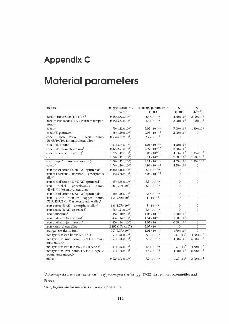
Appendix C

Material parameters

material† magnetisation Ms exchange parameter A K1 K2

(T (A/m)) (J/m) (J/m3) (J/m3)

barium iron oxide (1/12/19)1 0.48 (3.82×105) 6.3×10−12 4.50×105 3.00×105

barium iron oxide (1/12/19) room temper-ature2

0.48 (3.82×105) 6.3×10−12 3.20×105 1.00×105

cobalt1 1.79 (1.42×106) 3.02×10−11 7.00×105 1.80×105

cobalt(3) platinum3 1.38 (1.10×106) 9.93×10−12 2.00×106 0

cobalt iron nickel silicon boron(58/5/10/16/11) amorphous alloy4

0.53 (4.22×105) 2.7×10−12 0 0

cobalt platinum3 1.01 (8.04×105) 1.01×10−11 4.90×106 0

cobalt platinum chromium3 0.37 (2.94×105) 9.99×10−12 2.00×105 0

cobalt (room temperature)2 1.79 (1.42×106) 3.02×10−11 4.53×105 1.45×105

cobalt1 1.79 (1.42×106) 3.14×10−11 7.00×105 1.80×105

cobalt type 2 (room temperature)2 1.79 (1.42×106) 3.14×10−11 4.53×105 1.45×105

cobalt3 1.76 (1.40×106) 9.99×10−12 4.50×105 0

iron nickel boron (20/60/20) sputtered5 0.56 (4.46×105) 2.1×10−12 0 0

iron(40) nickel(40) boron(20) - amorphousalloy4

1.05 (8.36×105) 8.07×10−12 0 0


iron nickel phosphorous boron(40/40/14/6) amorphous alloy4

0.8 (6.37×105) 3.1×10−12 0 0


iron silicon niobium copper boron(73.5/13.5/3/1/9) nanocrystalline alloy6

1.2 (9.55×105) 1×10−11 0 0

iron boron (80/20) - amorphous alloy4 1.6 (1.27×106) 5×10−12 0 0

iron boron (80/20) sputtered5 1.56 (1.24×106) 5.4×10−12 0 0

iron palladium3 1.38 (1.10×106) 1.03×10−11 1.80×106 0

iron platinum (maximum)3 1.43 (1.14×106) 1.54×10−11 1.00×107 0

iron platinum (minimum)3 1.43 (1.14×106) 1.02×10−11 6.60×106 0

iron - amorphous alloy4 2.185 (1.74×106) 2.07×10−11 0 0

manganese aluminium3 0.7 (5.57×105) 1.02×10−11 1.70×106 0

neodymium iron boron (2/14/1)1 1.61 (1.28×106) 7.3×10−12 -1.80×107 4.80×107

neodymium iron boron (2/14/1) roomtemperature2

1.61 (1.28×106) 7.3×10−12 4.30×106 6.50×105

neodymium iron boron(2/14/1) type 21 1.61 (1.28×106) 8.4×10−12 -1.80×107 4.80×107

neodymium iron boron (2/14/1) type 2(room temperature)2

1.61 (1.28×106) 8.4×10−12 4.30×106 6.50×105

nickel1 0.62 (4.93×105) 7.2×10−12 -1.20×105 3.00×104

1Micromagnetism and the microstructure of ferromagnetic solids, pp. 17-22, first edition, Kronmuller and

Fahnle

2as 1; figures are for materials at room temperature

114

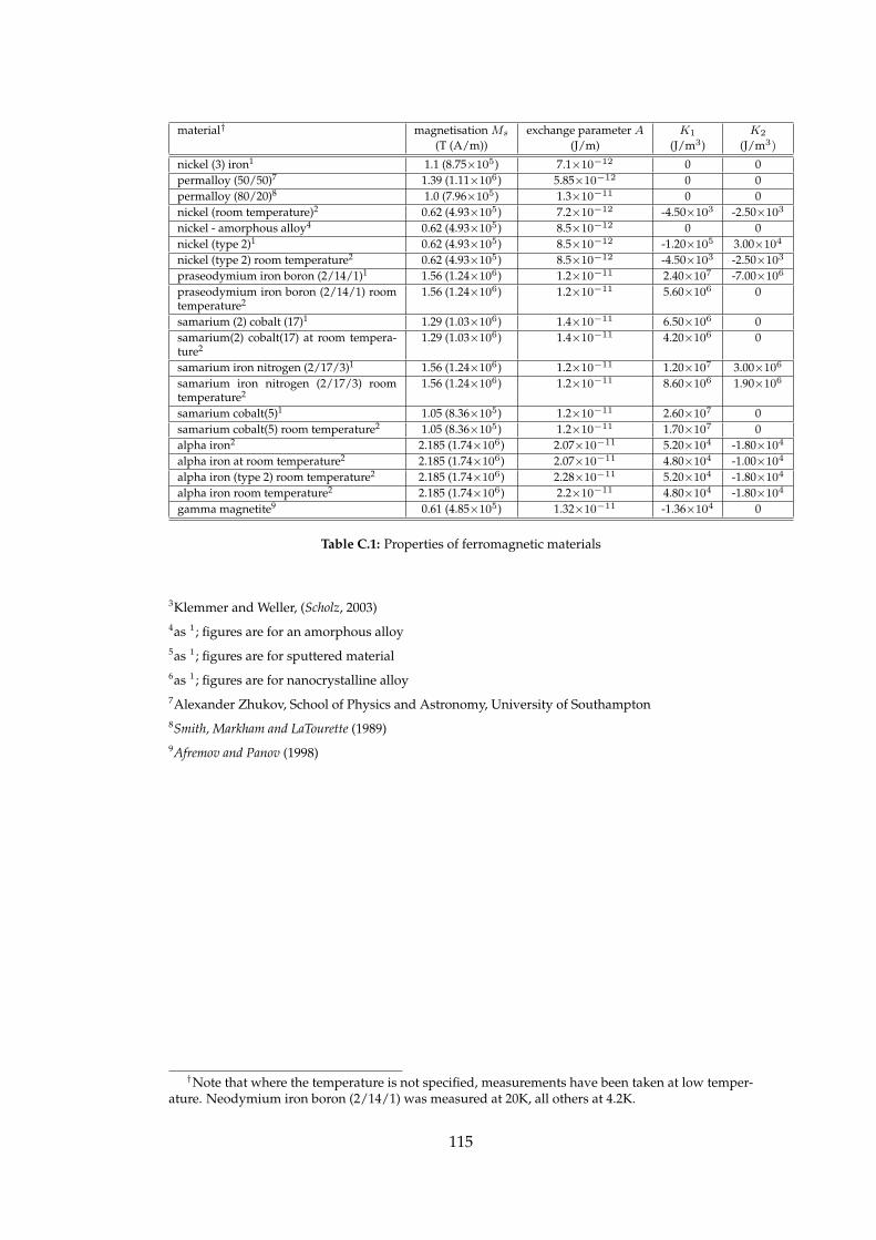
material† magnetisation Ms exchange parameter A K1 K2

(T (A/m)) (J/m) (J/m3) (J/m3)

nickel (3) iron1 1.1 (8.75×105) 7.1×10−12 0 0

permalloy (50/50)7 1.39 (1.11×106) 5.85×10−12 0 0

permalloy (80/20)8 1.0 (7.96×105) 1.3×10−11 0 0

nickel (room temperature)2 0.62 (4.93×105) 7.2×10−12 -4.50×103 -2.50×103

nickel - amorphous alloy4 0.62 (4.93×105) 8.5×10−12 0 0

nickel (type 2)1 0.62 (4.93×105) 8.5×10−12 -1.20×105 3.00×104

nickel (type 2) room temperature2 0.62 (4.93×105) 8.5×10−12 -4.50×103 -2.50×103

praseodymium iron boron (2/14/1)1 1.56 (1.24×106) 1.2×10−11 2.40×107 -7.00×106

praseodymium iron boron (2/14/1) roomtemperature2

1.56 (1.24×106) 1.2×10−11 5.60×106 0

samarium (2) cobalt (17)1 1.29 (1.03×106) 1.4×10−11 6.50×106 0

samarium(2) cobalt(17) at room tempera-ture2

1.29 (1.03×106) 1.4×10−11 4.20×106 0

samarium iron nitrogen (2/17/3)1 1.56 (1.24×106) 1.2×10−11 1.20×107 3.00×106

samarium iron nitrogen (2/17/3) roomtemperature2

1.56 (1.24×106) 1.2×10−11 8.60×106 1.90×106

samarium cobalt(5)1 1.05 (8.36×105) 1.2×10−11 2.60×107 0

samarium cobalt(5) room temperature2 1.05 (8.36×105) 1.2×10−11 1.70×107 0

alpha iron2 2.185 (1.74×106) 2.07×10−11 5.20×104 -1.80×104

alpha iron at room temperature2 2.185 (1.74×106) 2.07×10−11 4.80×104 -1.00×104

alpha iron (type 2) room temperature2 2.185 (1.74×106) 2.28×10−11 5.20×104 -1.80×104

alpha iron room temperature2 2.185 (1.74×106) 2.2×10−11 4.80×104 -1.80×104

gamma magnetite9 0.61 (4.85×105) 1.32×10−11 -1.36×104 0

Table C.1: Properties of ferromagnetic materials

3Klemmer and Weller, (Scholz, 2003)

4as 1; figures are for an amorphous alloy

5as 1; figures are for sputtered material

6as 1; figures are for nanocrystalline alloy

7Alexander Zhukov, School of Physics and Astronomy, University of Southampton

8Smith, Markham and LaTourette (1989)

9Afremov and Panov (1998)

†Note that where the temperature is not specified, measurements have been taken at low temper-ature. Neodymium iron boron (2/14/1) was measured at 20K, all others at 4.2K.

115

Appendix D

CGS and SI (MKS) unit systems

description cgs unit SI (mks) unit factor

acceleration galileo Gal metre per second squared m·s−2 0.01

dynamic viscosity poise P pascal second Pa·s 0.1

electric charge franklin Fr coulomb C 3.34×10−10

electric current biot Bi ampere A 10

electric dipole moment debye D coulomb metre C·m 3.34×10−30

energy (work) erg joule J 10−7

force dyne dyn newton N 10−5

heat energy calorie cal joule J 4.187

heat transmission langley kilojoule per square metre kJ·m−2 41.84

illumination phot ph lux lx 104

kinematic viscosity stokes St square metres per second m2·s−1 10−4

luminancelambert Lb

candela per square metre cd·m−2 3183.1

stilb sb 104

magnetic dipole moment emu ampere square metre A·m2 10−3

magnetic field strength oersted Oe ampere per metre A·m−1 79.577

magnetic flux

line li

weber Wb

10−8

maxwell Mx 10−8

unit pole 1.257×10−7

magnetic flux density gauss G tesla T 10−4

magnetomotive force gilbert Gi ampere A 0.796

permeability darcy square metre m2 0.987×10−12

pressure barye ba pascal Pa 0.1

wave number kayser K per metre m−1 100

Table D.1: The centimetre-gram-seconds (CGS) and the metre-kilogram-seconds (SI) unit systems.To convert from one system to the other, cgs unit × factor = mks unit. Data from Purcell(1985) and Jackson (1999)

116

Appendix E

Complete simulation process

This section discusses the complete simulation process, centred around the dia-

gram in figure E.1. This diagram shows the major supporting libraries, compilers,

interpreters, scripts, data stores and outputs of the method.

E.1 Notation

• Hexagonal boxes with green text indicate one of the two simulation packages

involved: OOMMF for the finite difference method, or magpar for the hybrid

finite element/boundary element method.

• Diamonds containing red text show a source compiler or a script interpreter,

such as gcc or Python.

• Parallelograms show a fundamental library necessary for the compilation of

one of the simulation packages.

• Ellipses with purple text show an intermediate data set necessary for “gluing”

components together.

• Boxes with blue text indicate a complex custom application designed to con-

vert or otherwise handle the input and output of one application or library.

• Trapezoids with grey text demonstrate a presentation output file; numerical

data

would be a hysteresis loop, for example, whereas graphical data would be

a magnetisation visualisation.

• Ellipsoids with red text show a supporting external application necessary for

visualisation, pre- or post-processing or runtime.

Conversion between data sets or to interpret a data set as the input of another

program is performed by a custom application not necessarily indicated on the

diagram in figure E.1 for clarity.

117

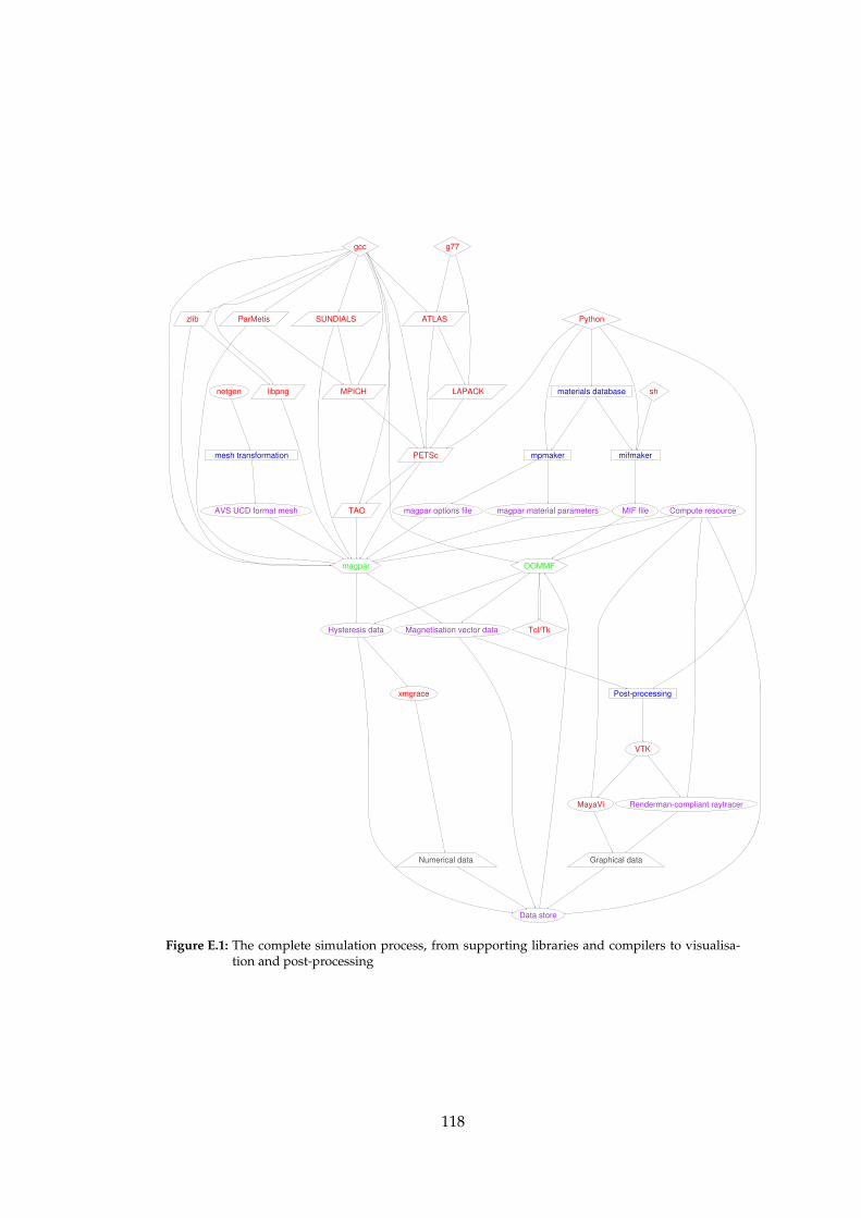
Python

mifmaker

Post-processing

materials database

mpmakerPETSc

MIF file

sh

OOMMF

Magnetisation vector dataHysteresis data Tcl/Tk

Data store

Compute resource

MayaVi Renderman-compliant raytracer

magpar

xmgrace

gcc

ATLAS

MPICH

ParMetis SUNDIALSzlib

TAO

libpng

VTK

Numerical data Graphical data

magpar options file magpar material parameters

LAPACK

g77

netgen

mesh transformation

AVS UCD format mesh

Figure E.1: The complete simulation process, from supporting libraries and compilers to visualisa-tion and post-processing

118

Problem Specification

Director

LLG Evolver

Driver

General Mesh

Energy

Tcl Control ScriptEvolver

Minimisation Evolver

Rectangular MeshSix Neighbour Exchange

Const Mag Demag

Uniaxial Anisotropy

Cubic Anisotropy

Figure E.2: The OOMMF extensible solver framework. Blue items in boxes indicate extensible areas

The build of the hybrid finite element/boundary element package magpar is

much more complicated than that of its finite difference peer, OOMMF. OOMMF is

available from the NIST website as either a source code package with a straightfor-

ward build process or as a precompiled binary application for many architectures

and operating systems, such as GNU/Linux or Microsoft Windows. The frame-

work of the three-dimensional micromagnetic problem solver, Oxs (the OOMMF

Extensible Solver), is shown in figure E.2. The blue items in boxes here show ar-

eas which can be straightforwardly extended to include, for example, a twenty-six

neighbour exchange energy contribution rather than the standard six neighbour ex-

change provided as standard with OOMMF. Oxs provides a powerful mechanism

for extending this micromagnetics package.

Conversely, magpar is dependent on many highly optimised mathematics li-

braries which have been developed by different organisations and individuals for

many years. While the result of each of these is a library which is extremely power-

ful with respect to its individual application (linear algebra, matrix transformation,

differential equation solvers), compatibility and ease-of-use suffer. Although these

issues will be addressed in due course, it alienates many members of the physics

community as one must be familiar with software development in a UNIX-like en-

vironment to successfully use the software when provided in this form.

In theory, of course, binaries of magpar could be provided just as for OOMMF,

however given the automatic calibration and tuning of the mathematical libraries

involved, performance would be adversely affected, and there is no guarantee that

the results would be accurate. Taking advantage of the features provided by one

particular architecture can introduce dangerous imprecision when run on another

similar architecture, especially when considering floating point computation can-

cellation and round-off errors (Schulte and Swartzlander, 2000).

119

Appendix F

Constructive solid geometries

In order to create micromagnetic problem input sources, such as MIF files for

OOMMF or to describe boundaries for magpar’s finite element meshes, we need

to define the basic geometry of the problem.

A basic geometry is one described by a simple mathematical equation, and these

are generally accepted by three-dimensional graphics modellers to be primitives —

constructive solid geometries (CSGs) (see figure F.1). The primitives can be consid-

ered to be the set of spheres, torii, cylinders, cuboids, pyramids and cones, as well

as the associated two-dimensional shapes. By adding or removing conditions for

satisfying the equations, the shape can be modified. For example, if one considers

a sphere where the volume conditions are defined by:

x2 + y2 + z2 ≤ 1 (F.1)

where x, y and z are between −1 and 1 then it is straightforward to modify this

such that the conditions in equation F.1 are met and z ≤ 0, then a half-sphere is

produced. This could be called a Boolean shape because the resultant geometry

shows a “negative” cuboid has been cut away from the sphere. A section of a

sphere could be created as though two cuboids have been subtracted from it by, in

addition to satisfying the above equations, satisfying z ≥ −0.5. If this is satisfied,

and the conditions for a cone:

x2 + y2 ≤(

z + 1

2

)2

(F.2)

are also met, then a section of a cone results and so forth. By continuing in this

fashion, it is possible to use a handful of primitives to build more complex objects

and subsequently arrays of these objects (see figure F.1).

120

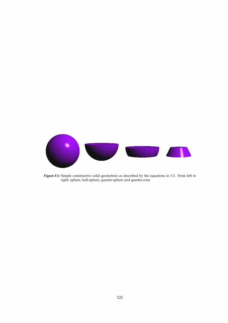
Figure F.1: Simple constructive solid geometries as described by the equations in 3.3. From left toright: sphere, half-sphere, quarter-sphere and quarter-cone

121

Bibliography

Afremov LL and Panov AV. Magnetic states and hysteresis properties of small

magnetite particles. Physics of Metals and Metallography, 86(3), 269–275 (1998).

Aharoni A. Magnetostatic energy of a ferromagnetic sphere. Journal of Applied

Physics, 51(11), 5906–5908 (1980).

Aharoni A. Magnetisation distribution in an ideally soft sphere. Journal of Applied

Physics, 55(4), 1049–1051 (1983).

Aharoni A. Introduction to the theory of Ferromagnetism. Oxford Science Publications,

2nd edition (2000).

Albrecht M, Ganesan S, Rettner CT, Moser A, Best ME, White RL and Terris BD.

Patterned perpendicular and longitudinal media: a magnetic recording study.

IEEE Transactions on Magnetics, 39(5), 2323–2325 (2003).

Argyres PN. Theory of the Faraday and Kerr effects in ferromagnetics. Physical

Review, 97(2), 334–345 (1955).

Baibich MN, Broto JM, Fert A, van Dau FN, Petroff F, Etienne P, Creuzet G,

Friederich A and Chazelas J. Giant magnetoresistance of (001)Fe/(001)Cr mag-

netic superlattices. Physical Review Letters, 61, 2472–2475 (1988).

Balay S, Buschelman K, Gropp WD, Kaushik D, Knepley M, McInnes LC, Smith

BF and Zhang H. PETSc users manual. Technical Report ANL-95/11 - Revision

2.1.5, Argonne National Laboratory (2002).

Balay S, Gropp WD, McInnes LC and Smith BF. Efficient management of paral-

lelism in object oriented numerical software libraries. In E Arge, AM Bruaset

and HP Langtangen, editors, Modern Software Tools in Scientific Computing, pages

163–202. Birkhauser Press (1997).

Ball S. Web Tcl Complete. McGraw-Hill (1999).

Barclay T, Chong W and Gray J. A quick look at serial ATA disk performance.

Technical Report MSR-TR-2003-70, Microsoft Research, Microsoft Corporation,

One Microsoft Way, Redmond, WA 98052 (2003).

122

Barthelmeß M, Pels C, Thieme A and Meier G. Stray fields of domains in permal-

loy microstructures — measurements and simulations. Journal of Applied Physics,

95(10), 5641–5645 (2004).

Barthelmeß M, Thieme A, Eiselt R and Meier G. Stray fields of iron electrodes for

spin-polarized transport. Journal of Applied Physics, 93, 8400 (2003).

Bartlett PN, Baumberg JJ, Birkin PR, Ghanem MA and Netti MC. Highly or-

dered macroporous gold and platinum films formed by electrochemical depo-

sition through templates assembled from submicron diameter monodisperse

polystyrene spheres. Chemistry of Materials, 14, 2199–2208 (2002).

Bartlett PN, Birkin PR and Ghanem MA. Electrochemical deposition of macrop-

orous platinum, palladium and cobalt films using polystyrene latex sphere tem-

plates. Chemical Communications, 17, 1671–1672 (2000).

Bartlett PN, Ghanem MA, de Groot PAJ and Zhukov AA. Method of producing

ordered arrays (2003a). UK Patent Application GB 0310498.1.

Bartlett PN, Ghanem MA, El Hallag IS, de Groot PAJ and Zhukov AA. Electrochem-

ical deposition of macroporous magnetic networks using colloidal templates.

Journal of Materials Chemistry, 13(10), 2596–2602 (2003b).

BBC. William Gilbert. http://www.bbc.co.uk/history/historic figures/

gilbert william.shtml (2004).

Bennett Goldberg I. 27 bits are not enough for 8-digit accuracy. Communications of

the ACM, 10(2), 105–106 (1967).

Bertram HN. Theory of Magnetic Recording. Cambridge University Press (1994).

Binnig G, Quate CF and Gerber C. Atomic force microscope. Physical Review Letters,

56(9), 930–933 (1986).

Binnig G and Rohrer H. The scanning tunneling microscope. Scientific American,

253, 40–46 (1985).

Binnig G, Rohrer H, Gerber C and Weibel E. Surface studies by scanning tunnelling

microscopy. Physical Review Letters, 49(1), 57–61 (1982).

Binnig G, Rohrer H, Gerber C and Weibel E. 7 x 7 reconstruction on Si(111) resolved

in real space. Physical Review Letters, 50(2), 120–123 (1983).

Blundell S. Magnetism in Condensed Matter. Oxford University Press, 1st edition

(2001).

123

Boardman RP, Fangohr H, Fairman MJ, Zimmermann J, Zhukov AA, Cox SJ and

de Groot PAJ. Micromagnetic modelling of ferromagnetic cones. Physical Review

B (2005a). Submitted.

Boardman RP, Fangohr H, Goncharov AV, Zhukov AA, de Groot PAJ and Cox SJ.

Micromagnetic simulation of ferromagnetic part-spherical particles. Journal of

Applied Physics, 95(11), 7037–7039 (2004).

Boardman RP, Zimmermann J, Fangohr H, Zhukov AA and de Groot PAJ. Mi-

cromagnetic simulation studies of ferromagnetic part-spheres. Journal of Applied

Physics, 97(10), 10E305 (2005b).

Bogomolov VN, Gaponenko SV, Germanenko IN, Kapitonov AM, Petrov EP, Gapo-

nenko NV, Prokofiev AV, Ponyavina AN, Silvanovich NI and Samoilovich SM.

Photonic band gap phenomenon and optical properties of artificial opals. Physi-

cal Review E, 55(6), 7619–7625 (1997).

Brown Jr. WF. Micromagnetics. Wiley Interscience, New York (1963).

C. H. Stapper J. Micromagnetic solutions for ferromagnetic spheres. Journal of

Applied Physics, 40(2), 798–802 (1969).

Chou SY. Patterned magnetic nanostructures and quantized magnetic disks. Pro-

ceedings of the IEEE, 85(4), 652–671 (1997).

Chou SY, Krauss PR and Kong L. Nanolithographically defined magnetic structures

and quantum magnetic disk. Journal of Applied Physics, 79(8), 6101–6106 (1996).

Cowburn RP. Property variation with shape in magnetic nanoelements. Journal of

Physics D: Applied Physics, 33, R1–R16 (2000).

Cowburn RP, Adeyeye AO and Bland JAC. Magnetic domain formation in litho-

graphically defined antidot permalloy arrays. Applied Physics Letters, 70(17),

2309–2311 (1997).

Cowburn RP, Adeyeye AO and Welland ME. Controlling magnetic ordering in

coupled nanomagnet arrays. New Journal of Physics, 1, 16 (1999a).

Cowburn RP, Koltsov DK, Adeyeye AO, Welland ME and Tricker DM. Single-

domain circular nanomagnets. Physical Review Letters, 83(5), 1042–1045 (1999b).

Curie P. Annales de Chimie et Physique, 5(289) (1895).

Dahlberg ED and Proksch R. Magnetic microscopies: the new additions. Journal of

Magnetism and Magnetic Materials, 200, 720–728 (1999).

Dao N, Whittenburg SL and Cowburn RP. Micromagnetics simulation of deep-

submicron supermalloy disks. Journal of Applied Physics, 90(10), 5235–5237 (2001).

124

de Groot PAJ. Private communication (2005).

Demmel J. Underflow and the reliability of numerical software. SIAM Journal of

Scientific and Statistical Computing, 5(4), 887–919 (1984).

Denkov ND, Velev OD, Kralchevsky PA, Ivanov IB, Yoshimura H and Nagayama

K. Two-dimensional crystallisation. Nature, 361(6407), 26 (1993).

Donahue MJ and McMichael RD. Exchange energy representational in computa-

tional micromagnetics. Physica B, 233, 272–278 (1997).

Donahue MJ and McMichael RD. Exchange energy representations in computa-

tional micromagnetics. Technical report, National Institute of Standards and

Technology, Gaithersburg, MD, USA (2002).

Donahue MJ and Porter DG. OOMMF User’s Guide. National Institute of Standards

and Technology, Gaithersburg, MD (1999). Interagency Report NISTIR 6376.

Eisenstein I and Aharoni A. Magnetisation curling in a sphere. Journal of Applied

Physics, 47(1), 321–328 (1975).

Flynt C. Tcl/Tk for Real Programmers. Academic Press International (1999).

Fruchart O, Nozieres JP, Wernsdorfer W, Givord D, Rousseaux F and Decanini

D. Enhanced coercivity in submicrometre-sized ultrathin epitaxial dots with in-

plane magnetisation. Physical Review Letters, 82, 1305–1308 (1999).

Gau H, Herminghaus S, Lenz P and Lipowsky R. Liquid morphologies on struc-

tured surfaces: from microchannels to microchips. Science, 283, 46–49 (1999).

Ghanem MA, Bartlett PN, de Groot PAJ and Zhukov A. A double templated elec-

trodeposition method for the fabrication of arrays of metal nanodots. Electro-

chemistry Communications, 6(5), 447–453 (2004).

Gilbert TL. A Lagrangian formulation of gyromagnetic equation of the magnetiza-

tion field. Physical Review, 100, 1243 (1955).

Gilbert W and Mottelay PF. De Magnete. Dover Publications (1600, 1991).

Goldberg D. What every computer scientist should know about floating-point

arithmetic. Computing Surveys (1991).

Gubbiotti G, Carlotti G, Nizzoli F, Zivieri R, Okuno T and Shinjo T. Magnetic prop-

erties of submicron circular permalloy dots. IEEE Transactions on Magnetics, 38(5),

2532–2534 (2002).

Ha JK, Hertel R and Kirschner J. Configurational stability and magnetization pro-

cesses in submicron permalloy disks. Physical Review B, 67, 064418 (2003).

125

Hehn M, Ounadjela K, Bucher JP, Rousseaux F, Decanini D, Bartenlian B and Chap-

pert C. Nanoscale magnetic domains in mesoscopic magnets. Science, 272, 1782–

1785 (1996).

Hetland ML. Practical Python. Apress, 1st edition (2002).

Hoinville J, Bewick A, Gleeson D, Jones R, Kasyutich O, Mayes E, Nartowski A,

Warne B, Wiggins J and Wong K. High density magnetic recording on protein-

derived nanoparticles. Journal of Applied Physics, 93, 7187–7189 (2003).

Huang Z. High accuracy numerical method of thin-film problems in micromagnet-

ics. Technical report, Department of Mathematical Sciences, Tsinghua University,

Beijing, 100084, P. R. China (2003).

Hubert A and Schafer R. Magnetic Domains. Springer - Verlag Berlin Heidelberg

(1998, 2000).

Hug HJ, Stiefel B, van Schendel PJA, Moser A, Hofer R, Martin S, Guntherodt HJ,

Porthun S, Abelmann L, Lodder JC, Bochi G and O’Handley RC. Quantitative

magnetic force microscopy of perpendicularly magnetized samples. Journal of

Applied Physics, 83(11), 5609–5619 (1998).

IBM. Alternative Storage. http://www.almaden.ibm.com/sst/storage/

alternative storage/pm.shtml (2002). IBM Almaden Research Centre.

IEEE. 754-1985 IEEE standard for binary floating-point arithmetic. Technical report,

Institute of Electrical and Electronics Engineers (1985).

Jackson JD. Classical Electrodynamics. Wiley, 3rd edition (1999).

Kittel C. Introduction to Solid State Physics. John Wiley and Sons, Inc., 7th edition

(1996).

Knuth DE. The Art of Computer Programming: Seminumerical Algorithms, volume 2.

Addison-Wesley, 3rd edition (1998).

Koltsov DK, Cowburn RP and Welland ME. Micromagnetics of ferromagnetic equi-

lateral triangular prisms. Journal of Applied Physics, 88(9), 5315–5317 (2000).

Kronmuller H and Fahnle M. Micromagnetism and the Microstructure of Ferromagnetic

Solids. Cambridge University Press, 1st edition (2003).

Lam J. Magnetic hysteresis of a rectangular lattice of interacting single-domain

ferromagnetic spheres. Journal of Applied Physics, 72(12), 5792–5798 (1992).

Landau LD and Lifshitz EM. On the theory of the dispersion of magnetic per-

meability in ferromagnetic bodies. Physikalische Zeitschrift der Sowjetunion, 8(2),

153–169 (1935).

126

Li SP, Natali M, Lebib A, Pein A, Chen Y and Xu YB. Magnetic nanostructure

fabriction by soft lithography and vortex-single domain transition in co dots.

Journal of Magnetism and Magnetic Materials, 241, 447–452 (2002).

Litzkow M. Remote UNIX - turning idle workstations into cycle servers. In Usenix

Summer Conference, pages 381–384 (1987).

Litzkow M, Livny M and Mutka M. Condor - a hunter of idle workstations. In 8th

International Conference of Distributed Computing Systems, pages 104–111 (1988).

Lutz M and Ascher D. Learning Python. O’Reilly, 2nd edition (2003).

Martın JL, Nogues J, Liu K, Vicent JL and Schuller IK. Ordered magnetic nanos-

tructures: fabrication and properties. Journal of Magnetism and Magnetic Materials,

256(1-3), 449–501 (2003).

Mayes E, Bewick A, Gleeson D, Hoinville J, Jones R, Kasyutich O, Nartowski A,

Warne B, Wiggins J and Wong KKW. Biologically derived nanomagnets in self-

organized patterned media. IEEE Transactions on Magnetics, 39, 624–627 (2003).

McVitie S, White GS, Scott J, Warin P and Chapman JN. Quantitative imaging of

magnetic domain walls in thin films using Lorentz and magnetic force micro-

scopies. Journal of Applied Physics, 90(10), 5220–5226 (2001).

O’Handley RC. Modern Magnetic Materials: Principles and Applications. John Wiley

and Sons, Inc. (1999).

Paine TO, Mendelsohn LI and Luborsky FE. Effect of shape anisotropy on the co-

ercive force of elongated single-magnetic-domain iron particles. Physical Review,

100, 1055–1059 (1955).

Pixar. The RenderMan Interface Specification v3.1 (1989).

Pixar. The RenderMan Interface Specification v3.2 (2000).

Purcell EM. Electricity and Magnetism, volume 2. Berkeley Physics, 2nd edition

(1985).

Raines P and Tranter J. Tcl/Tk in a nutshell. O’Reilly and Associates, Inc. (1999).

Ramachandran P. MayaVi: a free tool for CFD data visualisation. In 4th Annual

CFD Symposium, Aeronautical Society of India (2001).

Ramey C. Bash website (2003). www.gnu.org/software/bash/bash.html.

Ridge D, Becker D, Merkey P and Sterling T. Beowulf: Harnessing the power of

parallelism in a pile-of-PCs. Proceedings, IEEE Aerospace (1997).

127

Ross CA. Patterned magnetic recording media. Annual Review of Materials Research,

31, 203–235 (2001).

Ross CA, Farhoud M, Hwang M, Smith HI, Redjdal M and Humphrey FB. Micro-

magnetic behaviour of conical ferromagnetic particles. Journal of Applied Physics,

89(2), 1310–1319 (2001).

Rugar D, Marmin HJ, Guethner P, Lambert SE, Stern JE, McFadyen I and Yogi T.

Magnetic force microscopy: general principles and application to longitudinal

recording media. Journal of Applied Physics, 68(3), 1169–1183 (1990).

Saenz JJ, Garcia N, Grutter P, Meyer E, Heinzelmann H, Wiesendanger R, Rosen-

thaler L, Hidber HR and Guntherodt HJ. Observation of magnetic forces by the

atomic force microscope. Journal of Applied Physics, 62(10), 4293–4295 (1987).

Sanders IL, Kane SM and Cohen MS. 1µm bubble permalloy contiguous disk de-

vices. Journal of Applied Physics, 52(3), 2374–2376 (1981).

Schoberl J. Netgen 4.3 User’s Guide. http://www.hpfem.jku.at/netgen/ng4.pdf

(2003).

Scholz W. Scalable parallel micromagnetic solvers for magnetic nanostructures. Ph.D.

thesis, Fakultat fur Naturwissenschaften und Informatik, Technische Universitat

Wien (2003).

Scholz W, Fidler J, Schrefl T, Suß D, Dittrich R, Forster H and Tsiantos V. Scalable

parallel micromagnetic solvers for magnetic nanostructures. Computational Ma-

terials Science, 28, 366–383 (2003a).

Scholz W, Guslienko KY, Novosad V, Suß D, Schrefl T, Chantrell RW and Fidler J.

Transition from single-domain to vortex state in soft magnetic cylindrical nan-

odots. Journal of Magnetism and Magnetic Materials, 266, 155–163 (2003b).

Schroeder WJ, Martin KM and Lorensen WE. The design and implementation

of an object-oriented toolkit for 3D graphics and visualization. In R Yagel and

GM Nielson, editors, IEEE Visualization ’96, pages 93–100 (1996).

Schroeder WJ, Martin KM and Lorensen WE. The Visualisation Toolkit (VTK): An

object-oriented approach to 3D graphics. Pearson Education (1997).

Schulte MJ and Swartzlander Jr. EE. A family of variable-precision interval arith-

metic processors. IEEE Transactions on Computers, 49(5), 1–11 (2000).

Seberino C and Bertram HN. Concise, efficient three-dimensional fast multipole

method for micromagnetics. IEEE Transactions on Magnetics, 37, 1078–1086 (2001).

128

Skomski R and Coey JMD. Permanent Magnetism. Series in Condensed Matter

Physics. Institute of Physics (1999).

Smith C. [incr Tcl/Tk] from the ground up. Osborne (2000).

Smith N, Markham D and LaTourette D. Magnetoresistive measurement of the

exchange constant in varied-thickness permalloy films. Journal of Applied Physics,

65(11), 4362–4365 (1989).

Snir M, Otto SW, Huss-Lederman S, Walker DW and Dongarra J. MPI: the complete

reference. MIT Press (1995).

Stoner EC and Wohlfarth EP. A mechanism of magnetic hysteresis in heterogeneous

alloys. Philosophical Transactions of the Royal Society London, A240, 599–642 (1948).

Suß D. Micromagnetic simulations of antiferro- and ferromagnetic structures for mag-

netic recording. Ph.D. thesis, Fakultat fur Naturwissenschaften und Informatik,

Technischen Universitat Wien (2002).

Tarnopolsky GJ. Hard disk drive capacity at high magnetic areal density. IEEE

Transactions on Magnetics, 40(1), 301–306 (2004).

Teherani S, Chen E, Durlam M, de Herrera M, Slaughter JM, Shi J and Kerszykowski

E. High density submicron magnetoresistive random access memory. Journal of

Applied Physics, 85(8), 5822–5827 (1999).

Tsang C, Chen MM and Yogi T. Gigabit-density magnetic recording. Proceedings of

the IEEE, 81(9), 1344–1359 (1993).

Tsang C, Chen MM, Yogi T and Ju K. Gigabit density recording using dual-element

mr/inductive heads on thin-film disks. IEEE Transactions on Magnetics, 26(5),

1689–1693 (1990).

Turner PJ. Grace home. http://plasma-gate.weizmann.ac.il/Grace/ (1995).

van Rossum G. Python website (2003). http://www.python.org.

van Rossum G and Drake FL. Python Reference Manual. PythonLabs, Virginia, USA

(2001).

Van Roy W, Carpi EL, Van Hove M, Van Esch A, Bogaerts R, De Boeck J and Borghs

G. Study of the demagnetisation and optimisation of the magnetic field of per-

pendicular ferromagnetic thin films using sub-µm lithography. Journal of Mag-

netism and Magnetic Materials, 121(1-3), 197–200 (1993).

Velev OD and Kaler EW. In situ assembly of colloidal particles into miniaturised

biosensors. Langmuir, 15(11), 3696–3698 (1999).

129

Vlasov YA, Bo XZ, Sturm JC and Norris DJ. On-chip natural assembly of silicon

photonic bandgap crystals. Nature, 414, 289–293 (2001).

Wachowiak A, Wiebe J, Bode M, Pietzsch O, Morgenstern M and Wiesendanger R.

Direct observation of internal spin structure of magnetic vortex cores. Science,

298, 577–580 (2002).

Walker D. Standards for message passing in a distributed memory environment.

Technical report, Oak Ridge National Laboratory (1992).

Welch BB. Practical programming in Tcl and Tk. Prentice Hall PTR, 3rd edition (1999).

Wood RW. The feasibility of magnetic recording at 1 terabit per square inch. IEEE

Transactions on Magnetics, 36(1), 36–42 (2000).

Wood RW, Miles J and Olson T. Recording technologies for terabit per square inch

systems. IEEE Transactions on Magnetics, 38(4), 1711–1718 (2002).

Xu L, Zhou WL, Frommen C, Baughman RH, Zakhidov AA, Malkinski L, Wang

JQ and Wiley JB. Electrodeposited nickel and gold nanoscale metal meshes with

potentially interesting photonic properties. Chemical Communications, 12, 997–998

(2000).

Zhukov AA. Private communication (2004).

Zhukov AA, Ghanem MA, Goncharov AV, Boardman RP, Novosad V, Karapetrov

G, Fangohr H, Bartlett PN and de Groot PAJ. Oscillatory thickness dependence of

the coercive field in magnetic 3d anti-dot arrays. Physical Review Letters (2004a).

Submitted; preprint at cond-mat/0406091.

Zhukov AA, Goncharov AV, de Groot PAJ, Ghanem MA, El-Hallag IS, Bartlett PN,

Boardman RP, Fangohr H, Novosad V and Karapetrov G. Oscillatory thickness

dependence of the coercive field in 3d anti-dot arrays from self-assembly. Journal

of Applied Physics (2004b). Submitted.

Zhukov AA, Goncharov AV, de Groot PAJ, P.N.Bartlett and M.A.Ghanem. Magnetic

anti-dot arrays from self-assembly template methods. Journal of Applied Physics,

93, 7322–7324 (2003).

130

computer simulation studies of magnetic nanostructures

Documents