computer programme to calculate emissions from road...

COPERT 4

Computer programme to calculate emissions from road transport

User manual (version 9.0)

Dimitrios Gkatzoflias, Chariton Kouridis, Leonidas Ntziachristos and Zissis Samaras

ETC/AEM

February 2012

1

Table of Contents 1 Introduction ............................................................................... 2

2 Requirements ............................................................................. 4 2.1 Software installed ...................................................................................... 4 2.2 Minimum hardware requirements ................................................................ 4

3 Installing COPERT 4 .................................................................... 5 3.1 Installation procedure ................................................................................ 5 3.2 Uninstall procedure .................................................................................... 5

4 Structure of the programme ........................................................ 7

5 Starting COPERT 4 ...................................................................... 8 5.1 Main menu items ....................................................................................... 9

5.1.1 File ........................................................................................................... 9 5.1.2 Country ................................................................................................... 22 5.1.3 Fleet Configuration ................................................................................... 28 5.1.4 Activity Data ............................................................................................ 40 5.1.5 Calculation Factors .................................................................................... 43 5.1.6 Emissions ................................................................................................ 50 5.1.7 Advanced ................................................................................................ 55 5.1.8 Help ....................................................................................................... 66

6 Contact ..................................................................................... 70

2

1 Introduction COPERT 4 is a Microsoft Windows1 software program which is developed as a European tool for the calculation of emissions from the road transport sector. The emissions calculated include regulated (CO, NOx, VOC, PM) and unregulated pollutants (N2O, NH3, SO2, NMVOC speciation …) and fuel consumption is also computed. A detailed methodology supports the software application. For more information regarding the methodology, the user should consult the Methodology Report. COPERT 4 is an updated version of COPERT III including both revised methodological elements and a reworked user interface aiming at a compilation of complicated annual national inventories that include multiple countries and years in a single file. This manual discusses all advanced features. What's New in COPERT 4?

• User friendly environment • Multi-window environment • Minimal user effort during inventory process • Easy-to-use wizards • Developed with Microsoft Visual Studio .NET 2003 instead of Microsoft

Access (Runtime version of Access is no longer needed although data is stored in an Access file for backwards compatibility)

• Possibility for time-series in one file • Possibility of more than one scenario in a single file • Enhanced import/export capabilities (mainly Microsoft Excel) • Enhanced reports creation (formats: pdf, Microsoft Excel, Microsoft Word,

rtf) • Configuration of fleet (local/regional vehicle technologies) • Data can be changed at methodological level • Advanced Help features

New Methodological Features:

• Hot emission factors of regulated pollutants from conventional PCs and PTWs

• Hybrid vehicle fuel consumption and emission factors • New N2O/NH3 Emission Factors for PCs and LDVs • New corrections for emission degradation due to mileage • New Heavy duty vehicle and Buses methodology (emission factors, load

factor corrections and road gradient reductions) • New Mopeds and Motorcycles technologies • Developments on the cold-start emission front • Developments on evaporation losses incl. PTWs

This report is designed in order to help COPERT 4 users to produce in a short time a complete annual national emission data set from road transport. Hence, the manual is divided in several chapters. The different chapters include all information needed to build a complete data set, assuming that the user has no former experience in using COPERT 4 but he is quite familiar with the methodology and the terminology used. Background knowledge in using Microsoft Windows is also expected, although no special skills are required.

1 Microsoft, Microsoft Access, Excel, Word and Visual Studio .NET are registered trademarks and Windows and Windows NT are trademarks of Microsoft Corporation

3

Major attention has been given to ensure that no erroneous data are inserted. This can certify reasonable results. It cannot guarantee their accuracy though, if input data do not correspond to reality. This is a user responsibility. In order to be compatible with the application, this manual is designed in the same way that the software is developed. The contents in the manual are structured in the same order as the respective forms appear when preparing the inventory. Hence, it would be efficient to work with the program in parallel, as you read the manual. This is a rather tutorial use of this book. In any case, you can always refer to it for specific problems when you are quite acquainted with its use. The following coding is used throughout the manual:

• Bold characters refer to a menu item, button, tab or drop-down list, which you can click.

• Bold Inclined characters are used for fields in which you can click, enter, read or select values. Alternatively they can symbolise a file.

• Inclined characters refer to the application's forms. • Underlined characters are used only to emphasise the context

4

2 Requirements

2.1 Software installed COPERT 4 is a 32-bit application and 32-bit Microsoft Windows platform is required. Therefore, the software is not designed for operation in Windows 3.x environment. Minimum software requirements:

• Microsoft® Windows® 98 • or Microsoft Windows 98 Second Edition • or Microsoft Windows Millennium Edition (Windows Me) • or Microsoft Windows NT® 4 (Workstation or Server) with Service Pack 6a • or Microsoft Windows 2000 (Professional, Server, or Advanced Server)

with the latest Windows Service Pack and critical updates available from the Microsoft Security Web site

• or Microsoft Windows XP (Home or Professional) • or Microsoft Windows Vista (Home or Professional) • or Microsoft Windows 7 (Home or Professional) • or Microsoft Windows Server 2003 family • Microsoft Internet Explorer 5.01 or later • Microsoft .NET Framework v1.1 or later

2.2 Minimum hardware requirements

1) IBM2 – compatible computer Pentium 166 MHz3 2) 128Mb RAM4 3) Hard disk or network file server with 54 Mb free space

It has to be noted that a faster processor based computer and/or more on RAM memory are recommended if frequent use of the program is to be expected.

2 IBM is a registered trademark of International Business Machines Corporation 3 Or the minimum CPU required to run the operating system, whichever is higher 4 Or the minimum RAM required to run the operating system, whichever is higher

5

3 Installing COPERT 4

3.1 Installation procedure You can download the necessary installation files from the COPERT web site: http://www.emisia.com/copert/Download.html

1. Read the "License Agreement" and press 'Accept'. 2. Click on the button 'Download COPERT 4' and download one .zip file, the

'COPERT4v9_0.zip' (file size: ~16 Mb). 3. Extract the contents of the compressed .zip files in the same directory. A

temporary directory is recommended. 4. Double-click the extracted file setup.exe, to start the installation

procedure (Figure 1). 5. Follow the required steps of the installation. 6. After installation you may delete the .zip file. It is no longer needed to

complete the installation. Note: Microsoft .NET Framework v1.1 or later is required to install COPERT 4. You can also download the file from the COPERT web site or from Microsoft's web site. (file size 23.1 MB). This file should be downloaded and installed prior to installing COPERT 4 unless .NET Framework v1.1 or later is already installed on your computer.

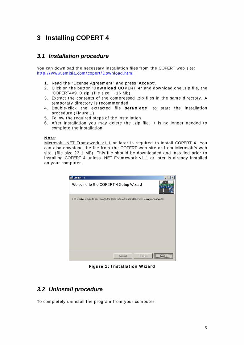
Figure 1: Installation Wizard

3.2 Uninstall procedure To completely uninstall the program from your computer:

http://www.emisia.com/copert/Download.html

http://lat.eng.auth.gr/copert/dotnetfx.exe

6

From the Control Panel of your Microsoft Windows system, double click the Add/Remove Programs icon. From the list select COPERT 4 and press Remove. A typical Windows uninstall procedure will follow. After doing so, COPERT 4 will have been completely removed from your computer.

7

4 Structure of the programme To have a better understanding of the programme use, it would be helpful to familiarise yourself also with its structure. This chapter helps you use the software more efficiently and take advantage of its special features. During the installation a folder COPERT 4 will be created into the Program Files folder of your Windows system. In this folder all the necessary files for the programme are located. Also a folder named COPERT 4 will be created in the folder: My Documents. In that folder a file named data.mdb will be placed. You can use this file for the first time you run COPERT 4 application, as it contains a sample run of Greece for the year 2005. Or you can create a new run with File>New and use the File>New Run Wizard for a guided walkthrough. When you open a file with the COPERT 4 application a copy of the file is created in the same folder of the opened file with an extension .tmpX, where X is a number. The copy-file is a hidden file. When you close the file from the File>Close menu or you try to exit the application you will be asked if you want the changes to be stored to the opened file. If you press Yes the changes will be stored and the copy file will be deleted. If you choose No the file will be deleted without storing the changes to the opened file. Note 1: If the application terminates abnormally the copy file is not deleted. You can delete it yourself. Also you can save your changes at any time from the menu File>Save to the same opened file or to another file from the menu File>Save As.... Note 2: When you open data.mdb for the first time you can save the data to another file (Save As…) and work with that file, so you will not modify the initial data.mdb file.

8

5 Starting COPERT 4 In order to start the COPERT 4 application, go to Start>All Programs>COPERT 4 from your Windows system taskbar and select COPERT 4. As soon as the application starts, the main interface appears (Figure 2). On the application's title the user can see that no file is open yet. Below the application's title, there is a main menu-bar of the programme and on the right side of the interface is a table which informs the user about the run details of the country and year he is processing. One can hide the run details table by pressing the Hide Run Details area, and press the Show Run Details area in order to view the table. This table's data change any time the user make any changes to the inventory file. So the user can see at any time what effect his changes take to the inventory process. Note: The user can open multiple forms at a time. All the forms will be placed into the main interface area. It is important to notice that changes can be made only to the first opened form. The other forms can be opened only for viewing information. This is done in order to keep consistency between the data that the user is viewing at any time.

Figure 2: The main interface of the programme

9

5.1 Main menu items The main menu items are: File, Country, Fleet Configuration, Activity Data, Calculation Factors, Emissions, Advanced and Help.

5.1.1 File This item provides all tools to manipulate all the inventory files. Under the File menu item (Figure 3) one can find the commands New, Open, Save, Save as…, Close, New Run Wizard, Import/Export, Reports and Exit.

Figure 3: File menu

File>New With this command the user can create a new run. A standard Windows popup form will appear. One can then specify a name for the run and a folder to save it in. The program will then create the proper ".mdb" file for storing the data of the new inventory. This may take a few seconds depending on the computer’s performance. The path of the new file will appear on the application's title-bar. File>Open If the user has previously created a run in COPERT 4 he can always view or edit the data by selecting the Open menu item. A standard Windows popup form will appear. Simply select the desired file or browse through the folders to locate it. By clicking the Open button the path of the new file will appear on the application's title-bar. Every time the user makes any change during the inventory process after the path of the file the word "(changed)" is added. If you save the file this word goes away. By default during the installation a COPERT 4 mdb file will be created in the My Documents folder, which can be used for the user's first run.

10

File>Save This command allows the user to save the current instance of the run anytime during the inventory preparation. All updates brought into the inventory up to this time will be saved and there is no way to retrieve data saved previously. File>Save as… If the user wishes to rename the inventory he is working on, or save it in a different folder, this option prompts the user to do so via a standard Windows popup form. By using this option one may create two versions of the same run and preserve data that were saved with the last File>Save command. File>Close This command closes the current inventory. Before closing, the programme prompts for saving the data. File>New Run Wizard After creating or opening an inventory file, one can use a wizard (Figure 4Figure 4), which performs the basic steps in order to calculate a complete run.

Figure 4: New Run Wizard

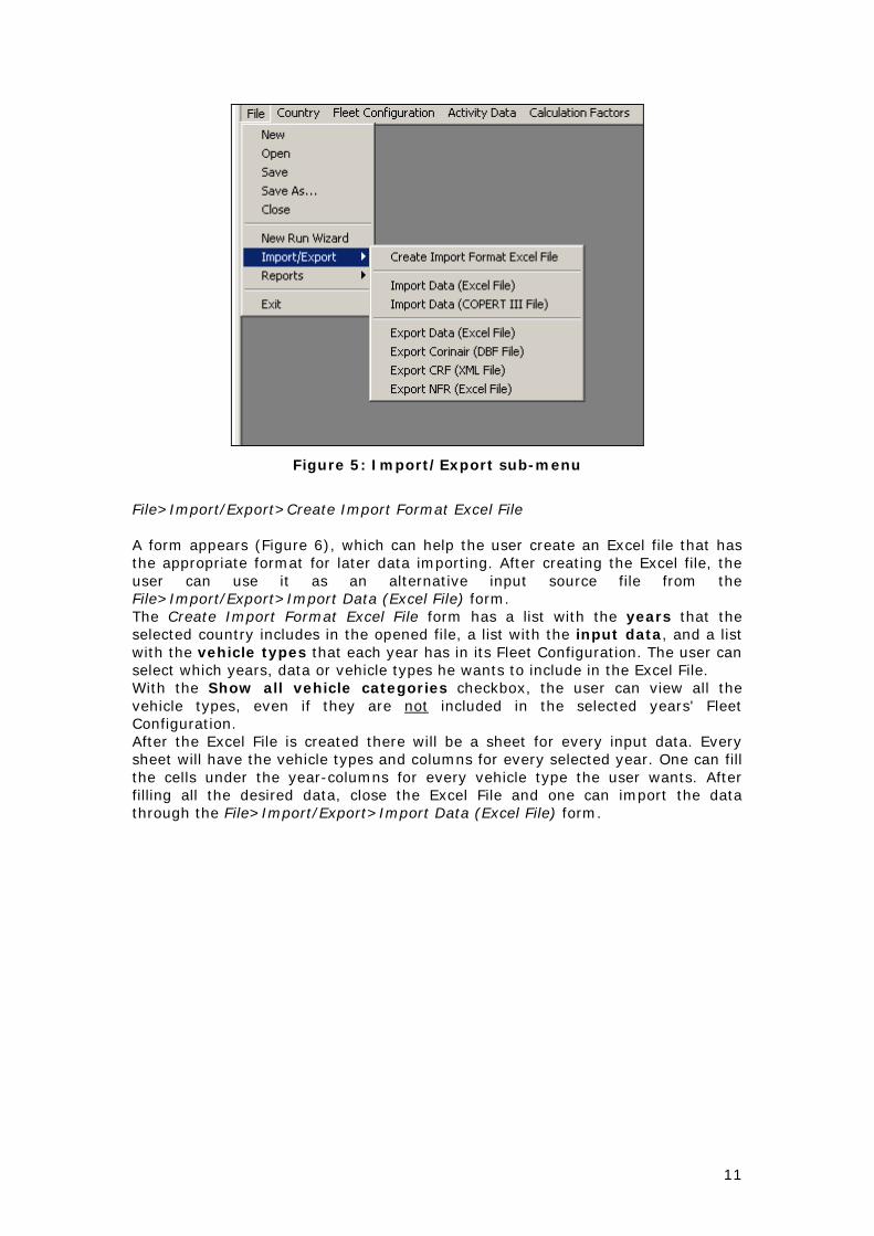
File>Import/Export After selecting a specific country from the Country>Select/Add form, one can import or export data, from and to the programme (Figure 5). The available options are: Create Import Format Excel File, Import Data (Excel File), Import Data (COPERT III file), Export Data (Excel File) , Export Corinair (DBF File) , Export CRF (XML File) , Export NFR (Excel File).

11

Figure 5: Import/Export sub-menu

File>Import/Export>Create Import Format Excel File A form appears (Figure 6), which can help the user create an Excel file that has the appropriate format for later data importing. After creating the Excel file, the user can use it as an alternative input source file from the File>Import/Export>Import Data (Excel File) form. The Create Import Format Excel File form has a list with the years that the selected country includes in the opened file, a list with the input data, and a list with the vehicle types that each year has in its Fleet Configuration. The user can select which years, data or vehicle types he wants to include in the Excel File. With the Show all vehicle categories checkbox, the user can view all the vehicle types, even if they are not included in the selected years' Fleet Configuration. After the Excel File is created there will be a sheet for every input data. Every sheet will have the vehicle types and columns for every selected year. One can fill the cells under the year-columns for every vehicle type the user wants. After filling all the desired data, close the Excel File and one can import the data through the File>Import/Export>Import Data (Excel File) form.

12

Figure 6: Create Import Format Excel File form

File>Import/Export>Import Data (Excel File) A form appears (Figure 7), which helps the user import data to the selected country from an Excel file that has the format of the file created by the File>Import/Export>Create Import Format Excel File form. During the process the programme informs the user about the data imported in the Results text-area.

13

Figure 7: Import Data (Excel File) form

File>Import/Export>Import Data (COPERT III file) With this form (Figure 8) the user can import data to the selected country and year from a run of COPERT III. Be careful first to have your fleet configured for the selected country and year, or else no input data will be imported. Pressing the Import 'COPERT III' Access File a standard Windows popup form will appear. Simply select the desired COPERT III file or browse through the folders to locate it. By clicking the Open button the import process will begin. During the process the programme informs the user about the data imported in the Results text-area. Data imported from COPERT III include:

1. Activity Data (Fleet, Mileage …) 2. Usage Data (Speeds, Shares) 3. Evaporation Data (Evaporation Share, Fuel RVP) 4. Temperatures and average daily trip distance

Since there is a new HDV classification in COPERT 4, Heavy Duty Trucks and Buses will not be imported during this process. For more information on how to import them please refer to the following link: http://www.emisia.com/versions/copert3.html under 'Information' and 'Datasheet with conversion'.

http://www.emisia.com/versions/copert3.html

14

Figure 8: Import Data (COPERT III file) form

File>Import/Export>Export Data (Excel File) A form appears (Figure 9), which can help the user create an Excel file with the same format of the files created by File>Import/Export>Create Import Format Excel File form, including results data. After creating the Excel file, the user can also use it as an alternative input source file from the File>Import/Export>Import Data (Excel File) form. The Export Data (Excel File) form has a list with the years that the selected country includes in the opened file, a list with the input data, a list with the results data, and a list with the vehicle types that each year has in the Fleet Configuration. The user can select which years, data or vehicle types he wants to include in the Excel File. With the Show all vehicle categories checkbox, the user can view all the vehicle types, even if they are not included in the selected years' Fleet Configuration. After the Excel File is created there will be a sheet for every input data and results data. Every sheet will have the vehicle types and columns for every selected year. One can alter the cells of the input data under the year-columns for every vehicle type the user wants. After updating all the desired data, close the Excel File and one can import the data through the File>Import/Export>Import Data (Excel File) form. If one wants to import data from one year to another one, alter the year-column value in all the desired sheets of the Excel file that one wants to import.

15

Figure 9: Export Data (Excel File) form

File>Import/Export>Export Corinair (DBF File) This form (Figure 10) exports the current inventory into two files COP_ACT.DBF and COP_EF.DBF which include the activity data and the emission factors respectively. Those files can then be introduced in CollectER via ImportER to link results calculated with COPERT 4 with the complete national inventory. The user can select for which years of the selected country, the appropriate files will be created. When the user presses Export a form will open, where the user can select where the files will be placed. For each year selected, a folder with the files will be created.

16

Figure 10: Export Corinair (DBF File) form

File>Import/Export>Export CRF (XML File) This form (Figure 11) is used to create an XML file that can be imported in CRF Reporter. Please follow the instructions in the Important Info area.

Figure 11: Export CRF (XML File) form

17

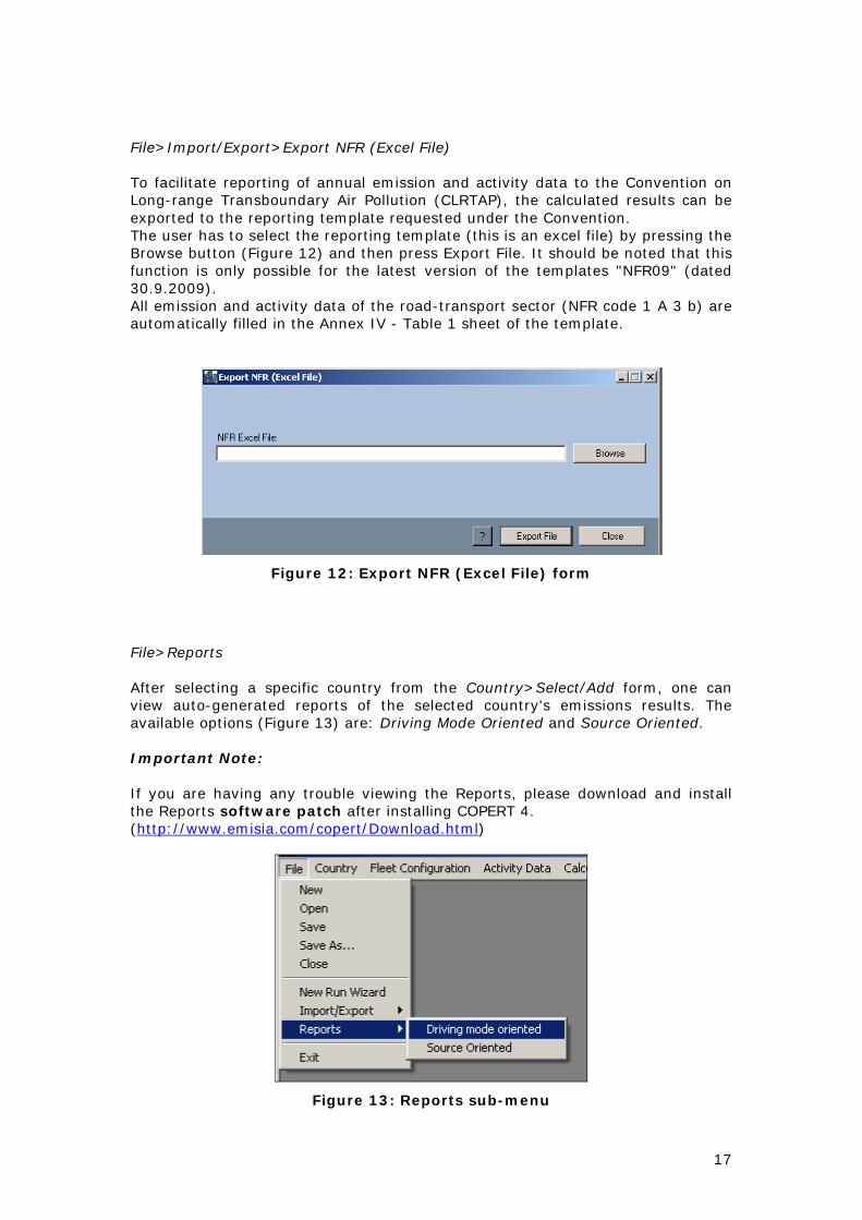
File>Import/Export>Export NFR (Excel File) To facilitate reporting of annual emission and activity data to the Convention on Long-range Transboundary Air Pollution (CLRTAP), the calculated results can be exported to the reporting template requested under the Convention. The user has to select the reporting template (this is an excel file) by pressing the Browse button (Figure 12) and then press Export File. It should be noted that this function is only possible for the latest version of the templates "NFR09" (dated 30.9.2009). All emission and activity data of the road-transport sector (NFR code 1 A 3 b) are automatically filled in the Annex IV - Table 1 sheet of the template.

Figure 12: Export NFR (Excel File) form

File>Reports After selecting a specific country from the Country>Select/Add form, one can view auto-generated reports of the selected country's emissions results. The available options (Figure 13) are: Driving Mode Oriented and Source Oriented. Important Note: If you are having any trouble viewing the Reports, please download and install the Reports software patch after installing COPERT 4. (http://www.emisia.com/copert/Download.html)

Figure 13: Reports sub-menu


18

File>Reports>Driving Mode Oriented With this form (Figure 14) the user can view, save and print reports with the emissions results of the selected country, oriented by driving mode (Urban, Rural, and Highway). The results are grouped by pollutant and the user can view all the years' results of the selected country. After each year two pie-charts follow concerning the year's results (Figure 15). After all the years for each pollutant, there are two bar-charts where the user can view the results during all the years (Figure 16). The user can navigate through the results, with the arrows on top of the form, or directly through the Group Tree section on the left side of the form. One can view the pages of a specific pollutant by double clicking on the shadowed box with the pollutant's name and a new tab will be created. One can export the pages of the tab (pdf, xls, doc or rtf format) that are viewed by clicking on the "envelope" icon. If someone wants to view specific years, select the desired years from the list-box on the right of the form and press Refresh Report.

Figure 14: Driving Mode Oriented report form

19

Figure 15: Pie-charts in the reports form

Figure 16: Bar-charts in the reports form

20

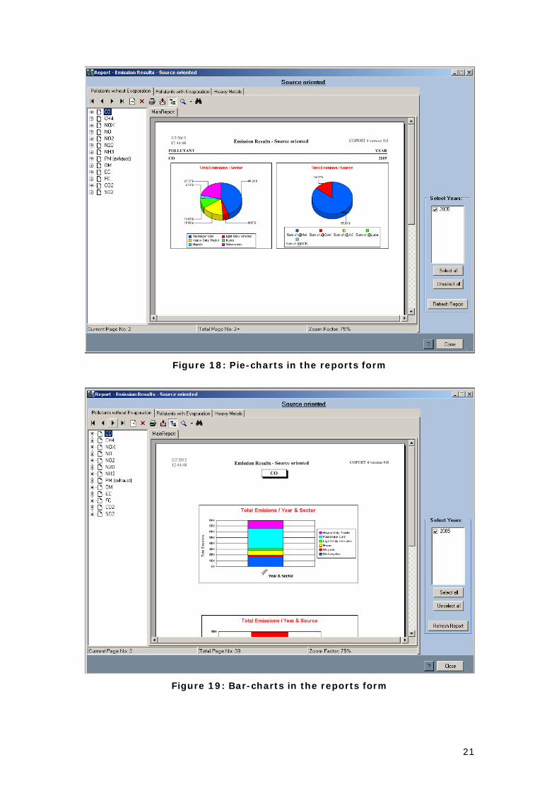
File>Reports>Source Oriented With this form (Figure 17) the user can view, save and print reports with the emissions results of the selected country, oriented by source (Hot, Cold start etc). The results are grouped by pollutant and the user can view all the years' results of the selected country. After each year two pie-charts follow concerning the year's results (Figure 18). After all the years for each pollutant, there are two bar-charts where the user can view the results during all the years (Figure 19). The user can navigate through the results, with the arrows on top of the form, or directly through the Group Tree section on the left side of the form. One can view the pages of a specific pollutant by double clicking on the shadowed box with the pollutant's name and a new tab will be created. One can export the pages of the tab (pdf, xls, doc or rtf format) that are viewed by clicking on the "envelope" icon. If someone wants to view specific years, select the desired years from the list-box on the right of the form and press Refresh Report.

Figure 17: Source Oriented report form

21

Figure 18: Pie-charts in the reports form

Figure 19: Bar-charts in the reports form

22

File>Exit With this command the user can exit the programme. Before exiting, the programme prompts for saving the data.

5.1.2 Country Under the Country menu (Figure 20), one can find the following commands: Select/Add, Edit, Delete, View All Run Details, Country Info, and Fuel Info.

Figure 20: Country menu

Country>Select/Add With this form (Figure 21) the user can select which inventory's country and year wants to process. One can also add a new country, or a new year for an existing country, by giving the country's name, year, Ltrip and t_trip (the mean driving duration per trip, average over the year) and pressing Add Data.

23

Figure 21: Select/Add Country and Year form

Country>Edit With this form (Figure 22) the user can change the countries' name, years, Ltrip and t_trip.

Figure 22: Edit Country's Attribures form

Country>Delete

24

With this form (Figure 23) the user can delete a country with all the years it has in the inventory file or a specific country's year. Be careful with this actions, because when someone deletes a country or a year, they will also be deleted their fleet configuration, activity data and all of their calculated factors and emissions.

Figure 23: Delete Country and/or Year(s) form

Country>View All Run Details With this form (Figure 24) the user can view all the run details for every country and year that the inventory file has.

Figure 24: View All Run Details form

Country>Country Info

25

In this form (Figure 25) the user has to provide values for monthly average minimum and maximum temperatures, RVP and Beta. The Beta values can also be calculated by pressing Calculate Beta. These values can be different for every country and year, but after the user makes any changes he will be asked if he wants to apply the changes to all the years of the selected country, or only to the selected year. RH (%) is the relative humidity per month. This is required to calculate the load of air-conditioning (A/C). A high value denotes high humidity and a higher load for the A/C that increases consumption.

Figure 25: Country Info form

Country>Fuel Info By selecting Fuel Info under the Country menu, a form appears (Figure 26) where the user has to provide data for the Fuel specifications and the Statistical Annual Fuel Consumption to be used in the calculations. The hydrogen to carbon atom ratio (H:C ratio) is also provided. Several values for heavy metal content and O:C ratio are proposed. However, those values can be changed if more accurate figures are available. These data can be different for every year and country. One can apply Fuel Correction by checking the Apply Statistical Fuel Correction checkbox. If zero values are provided in the Annual Fuel Consumption table then the user will be prompted if he is sure that he wants to apply fuel correction, although zero values are provided. Biodiesel Biodiesel use in Europe is increasing as a consequence of the biofuels promotion directive (2003/30/EC) and subsequent efforts. Currently, biodiesel is blended in almost all commercial diesel fuels in Europe at proportions that do not exceed 5% vol. Therefore, biodiesel is already used by possibly every single diesel vehicle in Europe, without the driver actually knowing it. As a result, biodiesel use is not limited to particular vehicle categories, such as the biodiesel busses in COPERT. The difference of the particular category is that these buses can operate at high biodiesel blending ratios (i.e. up to 30%),

26

without this affecting their operation. However, this affects their emission level, compared to normal busses. The user of COPERT should separately provide statistical fuel consumption values for conventional diesel (fossil diesel or petrodiesel) and biodiesel at a country level. In the fuel balance, the software adds petrodiesel and biodiesel and compares with the calculated fuel consumption. According to IPCC, tailpipe CO2 produced by the combustion of biofuels (in this case biodiesel) should not be included in the road transport total but should be included in the LULUCF sector. IPCC defines that CO2 from road transport should be determined on the basis of statistical fossil fuel consumption only. Therefore, if the user checks the “Statistical Fuel Correction” check-box, then CO2 is calculated only on the basis of the statistical fuel consumption of petrodiesel and not biodiesel. Therefore, in order to correctly report to CRF, the user needs to provide separately the diesel and biodiesel consumption values and check the “Apply Statistical Fuel Correction” check box.

Figure 26: Fuel Information

By pressing Provide Fuel Consumption in ...TJ the user can provide the energy conversion factors (Figure 27). Energy conversion factors are required to convert fuel consumption (t) used in COPERT to energy consumption (TJ) in order to report to UNFCCC. Alternatively, if energy consumption values are available from UNFCCC, these can be converted to fuel consumption by using the inverse energy conversion factors. According to the 2006 IPCC Guidelines for National Greenhouse Gas Inventories, the net (or lower) calorific value (NCV) should be used as the conversion factor for each fuel. The net calorific value is the total energy produced when one kg of

27

fuel is combusted and the combustion products are returned to ambient temperature. In simple words, is the energy availability of one kg of fuel. Liquid fuels used in transport are a mix of components. The mixing ratio depends on the fuel origin and processing for fossil-derived fuel, and the feedstock for biofuels. As a result, the exact NCV of each fuel also depends on origin and feedstock. A national survey in major refineries is required to obtain the exact NCV of fuels used in each country. For guidance, IPCC provides some default values for several fuels (Table 1.2 of the Introduction chapter in the 2006 IPCC Guidelines - Volume 2: Energy). However, these values appear not much relevant for European sources and biodiesel feedstocks. COPERT suggested values have been originated from the 2004 International Energy Association survey on NCVs and should be considered more appropriate for the European fuels. In particular for biodiesel, the NCV proposed corresponds to rapeseed oil derived biodiesel (RME), which is the major biodiesel feedstock in Europe. Different feedstocks will result to different NCVs. In any case, countries should make every effort to provide updated values based on national data, depending on the exact fuels used in each reporting year.

Figure 27: Energy Conversion Factors

By pressing Advanced the user can view and change the Improved Fuel Quality Specifications (Figure 28) and choose between three fuel types: 1996 (Base Fuel), 2000 (Stage 2000) and 2005 (Stage 2005) from the Year drop-down list. The default value is 1996. If this option is selected then all vehicles are assumed to operate on a conventional – Base – fuel (corresponding to 1996 EU15 market average). The introduction of improved Stage 2000 and Stage 2005 fuel types will have a positive effect not only on the corresponding vehicle technologies to be launched in 2000 and 2005 respectively but also to older vehicle technologies.

28

Figure 28: Improved Fuel Quality Specifications

5.1.3 Fleet Configuration Under this menu (Figure 29) the user can find commands to configure the fleet for every country and year, and manage all the type of vehicles that will be available in the inventory file. The following commands are available: Add/Delete Vehicles, Add New Type, Edit, and Delete User Defined.

Figure 29: Fleet Configuration menu

Fleet Configuration>Add/Delete Vehicles With this form (Figure 30) the user can select which types of vehicles will be in the fleet of selected country and year. The user can view all the sectors or a specific one using the Sector list-box. He can view all the types of vehicles that are available in the inventory file, or only the COPERT's default vehicles, or the user defined vehicles that were created with the Fleet Configuration>Add New Type wizard. The user can select which types of vehicles will take part in the fleet by double-clicking the Select checkbox of the desired vehicle. If the user wants to delete a vehicle from the fleet he can unselect it again by double-clicking the Select checkbox.

29

The Default Type column shows if the specific type of vehicle is a COPERT's default type or user defined. The user can also apply the fleet configuration to other years of the selected country by checking the years in the top right list. When the configuration is complete press OK and the appropriate data will be updated. This may take some time depending on the computer’s performance.

Figure 30: Add/Delete Vehicles form

Fleet Configuration>Add New Type With this command a wizard will begin that will help the user add a new type of vehicle in the inventory file. This type can later be used in every fleet configuration through the Fleet Configuration>Add/Delete Vehicles form. The following steps will be: Step 1: Select Sector Select the desired sector or add a new one (Figure 31).

30

Figure 31: Add New Type wizard (step 1)

Step 2: Select Subsector Select the desired subsector or add a new one (Figure 32).


Step 3: Select Technology Select the desired technology or add a new one. Do not forget to give the appropriate Euro number in the Euro No field (Figure 33). If this combination already exists the wizard cannot go on and the user will have to change one of his selections.

31


Step 4: Select Fuel Type Select the desired fuel type or add a new one (Figure 34).


Step 5: Finish Select the desired NMVOC category and whether the vehicle will take part in the Evaporation Calculations and press Finish to complete the wizard (Figure 35).

32


Fleet Configuration>Edit Under this menu (Figure 36) the user can use forms in order to edit sectors', subsectors' and technologies' names and the order of their appearance in all the data tables. The following forms are available: Sector, Subsector, and Technology.

Figure 36: Edit sub-menu

Fleet Configuration>Edit>Sector With this form (Figure 37) the user can change the "user defined" sectors' names by selecting the sector in the Properties tab, providing the new name in the Name textbox and pressing Change. In the Order tab the user can change the order of the sectors' appearance in all the data tables (Figure 38). In order to do that, change the number next to the sector. The sectors are sorted in ascending order according to this number.

33

Figure 37: Edit Sector form - Properties tab

Figure 38: Edit Sector form - Order tab

34

Fleet Configuration>Edit>Subsector With this form (Figure 39) the user can change the "user defined" subsectors' names by selecting the subsector in the Properties tab, providing the new name in the Name textbox and pressing Change. In the Order tab the user can change the order of the subsectors' appearance in all the data tables (Figure 40). In order to do that, change the number next to the subsector. The subsectors are sorted in ascending order according to this number.

Figure 39: Edit Subsector form - Properties tab

35

Figure 40: Edit Subsector form - Order tab

Fleet Configuration>Edit>Technology With this form (Figure 41) the user can change the "user defined" technologies' names by selecting the technology in the Properties tab, providing the new name in the Name textbox or a new euro number in the Euro No textbox and pressing Change. In the Order tab the user can change the order of the technologies' appearance in all the data tables (Figure 42). In order to do that, change the number next to the technology. The technologies are sorted in ascending order according to this number.

36

Figure 41: Edit Technology form - Properties tab

Figure 42: Edit Technology form - Order tab

37

Fleet Configuration>Delete User Defined Under this menu (Figure 43) the user can use forms in order to delete user defined sectors, subsectors, technologies and types of vehicles that were created with the Fleet Configuration>Add New Type wizard. The following forms are available: Type, Sector, Subsector, and Technology.

Figure 43: Delete User Defined sub-menu

Fleet Configuration>Delete User Defined>Type With this form (Figure 44) the user can delete user defined types of vehicles that were created with the Fleet Configuration>Add New Type wizard. One can view all the sectors at the same time or a specific one using the Sector list-box. One can select which types of vehicles will be deleted by double-clicking the Select checkbox of the desired vehicle and press Delete Selected Vehicle Categories. In order to delete them, they cannot be used in any of the fleet configurations of the inventory file. First one has to delete them from the Fleet Configuration>Add/Delete Vehicles form by unselecting them from all the countries and years that they are used.

38

Figure 44: Delete User Defined Type of Vehicle form

Fleet Configuration>Delete User Defined>Sector With this form (Figure 45) the user can delete user defined sectors that were created with the Fleet Configuration>Add New Type wizard. One can delete them by selecting them and pressing Delete. In order to delete them, they cannot be used in any of the user defined type of vehicles. First one has to delete those from the Fleet Configuration>Delete User Defined>Type form.

Figure 45: Delete User Defined Sector form

39

Fleet Configuration>Delete User Defined>Subsector With this form (Figure 46) the user can delete user defined subsectors that were created with the Fleet Configuration>Add New Type wizard. One can delete them by selecting them and pressing Delete. In order to delete them, they cannot be used in any of the user defined type of vehicles. First one has to delete those from the Fleet Configuration>Delete User Defined>Type form.

Figure 46: Delete User Defined Subsector form

Fleet Configuration>Delete User Defined>Technology With this form (Figure 47) the user can delete user defined technologies that were created with the Fleet Configuration>Add New Type wizard. One can delete them by selecting them and pressing Delete. In order to delete them, they cannot be used in any of the user defined type of vehicles. First one has to delete those from the Fleet Configuration>Delete User Defined>Type form.

40

Figure 47: Delete User Defined Technology form

5.1.4 Activity Data Under this menu (Figure 48) the user can provide fleet, circulation and evaporation data for the fleet configuration of the selected country and year. The available options are: Input Fleet Data, Input Circulation Data, and Input Evaporation Data.

Figure 48: Activity Data menu

Activity Data>Input Fleet Data In this form (Figure 49) the user can input data for Population, Annual Mileage (km/year) and Mean fleet mileage (km). The mean fleet mileage is relevant for both the calculation of evaporative emissions and the estimation of mileage degradation parameters. The Mean fleet mileage column is the mean cumulative fleet mileage in kilometres for each vehicle technology. In other words, the mean distance travelled by the fleet vehicles of the specific technology level since their introduction in the market. This value is then used to provide an emission degradation factor depending on vehicle age (or, total mileage driven).

41

To move between vehicle sectors use the Sector drop-down list.

Figure 49: Input Fleet Data form

Activity Data>Input Circulation Data In this form (Figure 50) the user can see the input form, aiming at collecting the average Speed and the mileage percentage driven by each vehicle technology per driving mode. To move between vehicle sectors use the Sector drop-down list.

42

Figure 50: Input Circulation Data form

Activity Data>Input Evaporation Data In this form (Figure 51) the user can input data for Fuel Tank Size (lt), Canister size, percentage of vehicles equipped with Fuel Injection (%), percentage of vehicles equipped with Evaporation Control (%) and the distribution of evaporative emissions to different driving modes (%) . To move between vehicle sectors use the Sector drop-down list.

Figure 51: Input Evaporation Data form

43

5.1.5 Calculation Factors Under this menu (Figure 52) the user can use forms, in order to calculate emission factors that will be used in the total emissions calculations. The available options are: Mileage Degradation, Fuel Effect, Hot Emission Factors, Cold Emission Factors, Evaporation Factors, A/C Factors and CO2 due to lube oil.

Figure 52: Calculation Factors menu

Calculation Factors>Mileage Degradation With this form (Figure 53) the user can calculate the mileage degradation factors, which are used to provide an emission degradation factor depending on vehicle age (or, total mileage driven). Relevant degradation factors are only given for EURO I and later passenger cars and light duty vehicles only and apply to hot emissions only. One can calculate the factors by pressing Recalculate Mileage Degradation Factors, and view the factors for each pollutant through the Pollutant drop-down list and for each sector through the Sector drop-down list.

44

Figure 53: Mileage Degradation Factors form

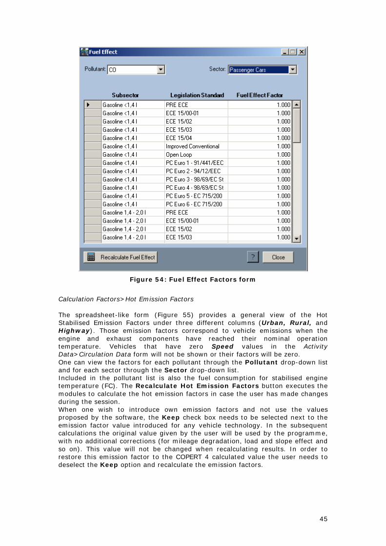
Calculation Factors>Fuel Effect The user can use this form (Figure 54), in order to calculate factors that take effect on the hot emission factors. One can calculate the factors by pressing Recalculate Fuel Effect, and view the factors for each pollutant through the Pollutant drop-down list and for each sector through the Sector drop-down list. Note that only if you press Recalculate Fuel Effect the fuel year that is selected under the Country>Fuel Info form will be applied.

45

Figure 54: Fuel Effect Factors form

Calculation Factors>Hot Emission Factors The spreadsheet-like form (Figure 55) provides a general view of the Hot Stabilised Emission Factors under three different columns (Urban, Rural, and Highway). Those emission factors correspond to vehicle emissions when the engine and exhaust components have reached their nominal operation temperature. Vehicles that have zero Speed values in the Activity Data>Circulation Data form will not be shown or their factors will be zero. One can view the factors for each pollutant through the Pollutant drop-down list and for each sector through the Sector drop-down list. Included in the pollutant list is also the fuel consumption for stabilised engine temperature (FC). The Recalculate Hot Emission Factors button executes the modules to calculate the hot emission factors in case the user has made changes during the session. When one wish to introduce own emission factors and not use the values proposed by the software, the Keep check box needs to be selected next to the emission factor value introduced for any vehicle technology. In the subsequent calculations the original value given by the user will be used by the programme, with no additional corrections (for mileage degradation, load and slope effect and so on). This value will not be changed when recalculating results. In order to restore this emission factor to the COPERT 4 calculated value the user needs to deselect the Keep option and recalculate the emission factors.

46

Figure 55: Hot Emission Factors form

Calculation Factors>Cold Emission Factors This spreadsheet-like form (Figure 56) follows the same principals as the Hot Emission Factors form. However, cold excess emission factors are temperature dependant and therefore an additional list of Month tabs (January to December) is given on the top of the form. The Keep checkbox is similar to that described in the Calculation Factors>Hot Emission Factors form. Since Excess cold emissions are initially attributed to urban driving only, assuming that the majority of vehicles start their trips from urban areas, only urban emission factors are proposed for cold start. The Recalculate Cold Emission Factors button executes the modules to calculate the cold emission factors in case the user has made changes during the session. One can view the factors for each pollutant through the Pollutant drop-down list and for each sector through the Sector drop-down list.

47

Figure 56: Cold Emission Factors form

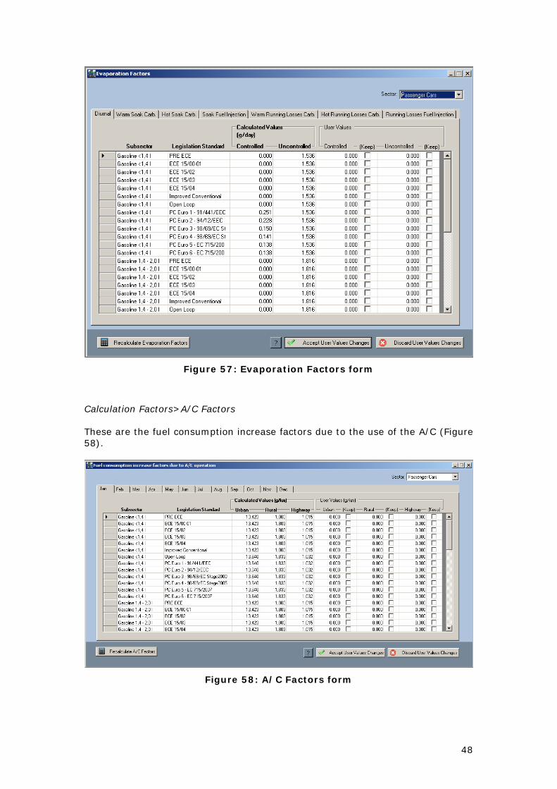
Calculation Factors>Evaporation Factors In this spreadsheet-like form (Figure 57) the user can edit the emission factors for fuel evaporation originating from different vehicle sources and covered by the seven tabs of the form. Those emission factors are only relevant for gasoline powered vehicles. Two columns are provided, proposing emission factors for vehicles equipped with evaporation control systems (Controlled) or without any control devices (Uncontrolled). Again, own emission factors may be preserved by selecting the Keep check box for any vehicle technology and evaporation source. The current methodology has superseded the Standard Corinair approach used in older COPERT versions and includes new emission factors based on a recent experimental dataset. The Recalculate Evaporation Factors button executes the modules to calculate the evaporation factors in case the user has made changes during the session. One can view the factors for each sector through the Sector drop-down list.

48

Figure 57: Evaporation Factors form

Calculation Factors>A/C Factors These are the fuel consumption increase factors due to the use of the A/C (Figure 58).

Figure 58: A/C Factors form

49

These are multiplied with the annual mileage per mode (urban, rural, highway), the usage factor and the number of vehicles equipped with A/C per technology, to calculate total the fuel consumption increase. Own emission factors may be preserved by selecting the Keep check box for any vehicle technology and month. The Recalculate A/C Factors button executes the modules to calculate the A/C factors in case the user has made changes during the session. One can view the factors for each sector through the Sector drop-down list. Calculation Factors> CO2 due to lube oil Lubricant oil is used in engines to reduce friction and to cool down specific components. Lube oil enters the combustion chamber and is oxidized during combustion, before it is exhausted to the atmosphere. The hydrocarbon composition of lube oil means that it unintentionally contributes to the CO2 emissions without taking part to the energy consumption of road transport. The only exception is two-stroke engines where the lube-oil is intentionally delivered to the cylinder and part of the lube oil could be used to deliver some energy to the engine (especially in older two-stroke engines). Emission factors of CO2 due to lube oil consumption per vehicle technology are provided in this form (Figure 59), which are based on typical lube-oil consumption factors for different vehicle types. These emission factors can be used "as is" unless there are better estimates. The user may also select whether lube oil consumption will be estimated in the total CO2 emissions or not (Add CO2 Emissions due to lube-oil (Yes/No)). Own emission factors may be preserved by selecting the Keep check box for any vehicle technology. One can view the factors for each sector through the Sector drop-down list.

Figure 59: CO2 due to lube oil

50

5.1.6 Emissions Under this menu item (Figure 60) the user can calculate and view results concerning the total emissions. The available options are: Total Emissions, Total Emissions of all years, Fuel Balance, NMVOC Speciation and NMVOC Speciation per vehicle type.

Figure 60: Emissions menu

Emissions>Total Emissions With this form (Figure 61) the user can calculate the total emissions for hot, cold, evaporation, A/C, Lube-oil and SCR emissions. With the Recalculate area one can calculate the Hot , Cold , Evaporation Emissions with the corresponding buttons in case the user has made changes during the session. With the All Emissions (including all factors) button one can calculate all the above emissions and the factors that are located under the Calculation Factors menu. After calculating the emissions the user can view the results using the corresponding tabs. One can view the emissions for each pollutant through the Pollutant drop-down list and for each sector through the Sector drop-down list. Important Notes: PM2.5 and PM10 total emissions and A/C, Lube-oil and SCR emissions are calculated by pressing the All Emissions (including all factors) button. When the user selects FC, CO2, SO2 and heavy metals the relevant tabs of A/C, Lube-oil and SCR emissions appear.

51

Figure 61: Total Emissions form

Emissions>Total Emissions of all years With this form (Figure 62) the user can view the total emissions of all the years of the selected country. Results are presented in tonnes for all major gaseous pollutants and in kg for heavy metals. The user can view the results based on the driving mode (Urban, Rural, and Highway) and the total ones. If a fleet configuration of a specific year does not have a specific vehicle, then the emission value appears as zero. One can view the emissions for each pollutant through the Pollutant drop-down list and for each sector through the Sector list-box.

52

Figure 62: Total Emissions of all years form

Emissions>Fuel Balance The fuel balance form (Figure 63) provides a control point to compare the statistical fuel consumption provided in the respective form Country>Fuel Info with the total fuel consumption calculated by the software application. The deviation between the two values should not exceed a few percentage units for the input data to be considered representative of their application. Therefore, this check can provide a verification of the overall accuracy of the input data and that no severe inconsistencies have been introduced into the calculations. If a significant deviation exists between the two values then you should make sure that the statistical fuel consumption has been introduced correctly and it corresponds to the real amount of fuel consumed by vehicles operating in the area selected for the inventory. If this figure is correct then some of the activity data need modifications. To obtain a better match between the statistical and calculated fuel consumption one may propose:

• Modify the mileage fraction allocated to different driving modes (Activity Data>Input Fleet Data form). Emission and consumption factors vary according to driving mode and therefore wrong estimations of the distance travelled under different conditions may provide an erroneous final result.

• Modify the speeds attributed to different driving modes. Speeds introduced in the relevant fields of the Activity Data>Input Circulation Data form correspond to the mean travelling speeds for the fleet of vehicles and have a significant influence on the emission and consumption factors.

• Make sure that the vehicle fleet has been correctly distributed to different vehicle technologies (Activity Data>Input Fleet Data form). Significant estimations may be necessary to adapt different national classification

53

(especially before Euro I vehicles) to the vehicle technology classification of COPERT 4. Since different vehicle technologies have both different emission and consumption factors, the particular allocation of vehicles has an impact on the also final result.

• Although the mileage driven per year has a linear effect on the total emissions, this should be a relevantly evident figure which accepts minor modifications. Moreover, values like monthly temperatures, RVP, etc. although have an effect on total emissions should not be changed because they should be considered much more reliable in comparison with those previously mentioned.

Figure 63: Fuel balance (statistical and calculated) results form

Additionally, it needs to be mentioned that emissions of fuel dependant pollutants (CO2, SO2, Heavy Metals) are calculated on the basis of the statistical fuel consumption. To do so, the total emissions, as calculated by COPERT 4 with application of the fuel consumption factors, are multiplied by the ratio Statistical/Total Calculated fuel consumption for each fuel type. In order to apply this correction, the statistical fuel consumption needs to be introduced (Country>Fuel Info form, Annual Fuel Consumption table). In case the relevant figures miss, the results are calculated on the basis of the calculated fuel consumption only. Naturally, this would mean that no statistical consumption figures exist for the specific fuel type, and therefore the fuel balance is not valid. Emissions>NMVOC Speciation This form (Figure 64) provides the total NMVOC speciation in different hydrocarbon species originating both from exhaust and evaporation emissions. The upper part of the form presents the emissions of open chain and aromatic hydrocarbons in [t] and the lower part the total emissions of PAHs and POPs (including furans and dioxins) in [g]. Please note that the speciation does not include 2-stroke engines and that, when summed up, the NMVOC species list gives a lower value than total NMVOC emissions because some of NMVOC is considered to be PAHs and POPs. The Recalculate NMVOC Speciation Results button executes the modules to calculate the emissions in case the user has made changes during the session.

54

Figure 64: NMVOC Speciation form

Emissions>NMVOC Speciation per vehicle type In this form (Figure 65), NMVOC speciation per vehicle type and substance is provided. You may select the species to be viewed in the left-hand side top drop-down form and the vehicle type from the right-hand side top drop-down form. Please note that the units that emissions are reported change depending on the species viewed. PAHs, POPs, Dioxins and Furans are reported in [g]. All other species are reported in [tn].

55

Figure 65: NMVOC speciation per vehicle type form

5.1.7 Advanced Under this menu (Figure 66) the user can provide the parameters for advanced features of COPERT that are not necessary for the compilation of a standard national inventory, but they are used to refine the results and provide additional sensitivity parameters implementing a more detailed description of the activity characteristics such as the load factor of the Heavy Duty Vehicles and the road gradient. The available options are: Vehicle Load, Axles, Road Slope, SCR usage, A/C usage, Share of NO2 to NOX, Fraction of EC and OM in PM and Parameters.

Figure 66: Advanced menu

56

Advanced>Vehicle Load, Axles The load percentage corrections (Figure 67) are applicable to heavy duty vehicles and buses and they depend on the vehicle gross weight class and driving mode. A default value of 50% is given and this corresponds to the baseline emission factors of COPERT. In order to apply a different load percentage the user needs to select the Yes option once he has made his changes. To remove the effect of different load percentages just select the No option. Needless to say that load percentages should range between 0 and 100 denoting a totally empty or a fully laden vehicle respectively. The load factors are calculated and applied during the calculation of the hot emission factors in the Calculation Factors>Hot Emission Factors form. Load percentages and the number of Axles are also used in the calculation of non-exhaust PM emissions in the Emissions>Total Emissions form.

Figure 67: Vehicle Load, Axles form

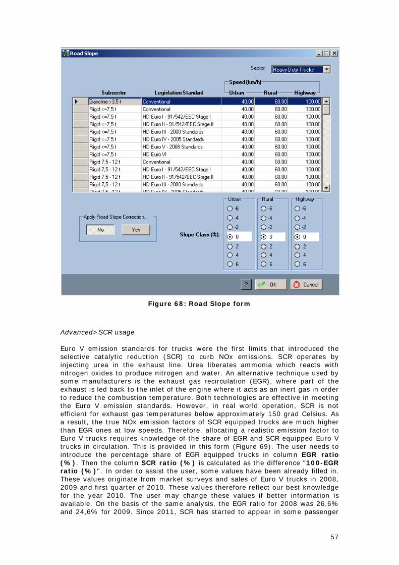
Advanced>Road Slope In this form (Figure 68) the user provides the mean gradient class of the road for different vehicle categories (HDV and Buses) and different driving modes. Select a vehicle category and then choose between 6 gradient classes ranging between -6% (uphill driving) to +6% (downhill driving) for every driving mode. The 0% slope value means that no changes will be made to the baseline emission factors (even road) even if the user has clicked the Yes button of the Apply Road Slope Correction area. The different road gradient corrections are only applicable for a limiting – and reasonable – speed range. The slope factors are calculated and applied during the calculation of the hot emission factors in the Calculation Factors>Hot Emission Factors form, as soon as Yes is selected.

57

Figure 68: Road Slope form

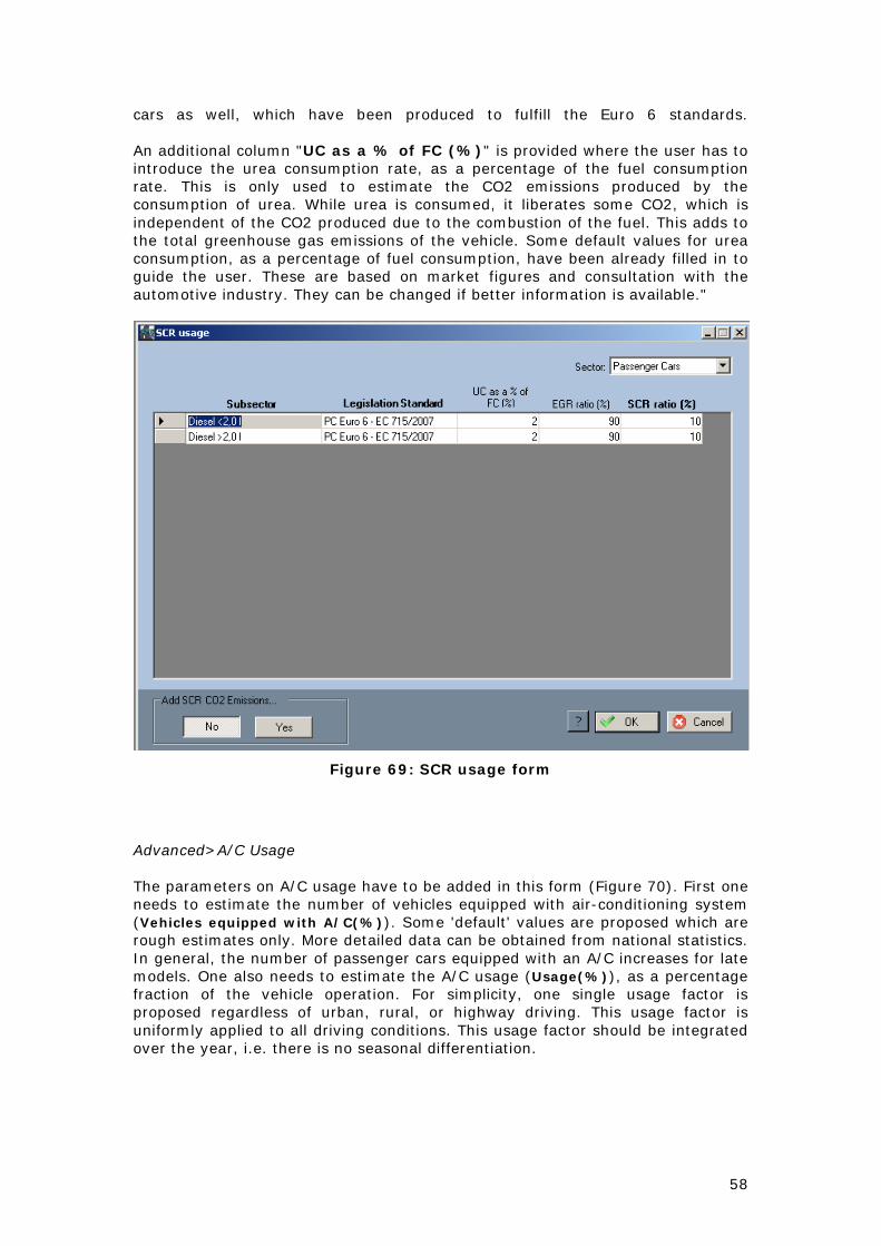
Advanced>SCR usage Euro V emission standards for trucks were the first limits that introduced the selective catalytic reduction (SCR) to curb NOx emissions. SCR operates by injecting urea in the exhaust line. Urea liberates ammonia which reacts with nitrogen oxides to produce nitrogen and water. An alternative technique used by some manufacturers is the exhaust gas recirculation (EGR), where part of the exhaust is led back to the inlet of the engine where it acts as an inert gas in order to reduce the combustion temperature. Both technologies are effective in meeting the Euro V emission standards. However, in real world operation, SCR is not efficient for exhaust gas temperatures below approximately 150 grad Celsius. As a result, the true NOx emission factors of SCR equipped trucks are much higher than EGR ones at low speeds. Therefore, allocating a realistic emission factor to Euro V trucks requires knowledge of the share of EGR and SCR equipped Euro V trucks in circulation. This is provided in this form (Figure 69). The user needs to introduce the percentage share of EGR equipped trucks in column EGR ratio (%). Then the column SCR ratio (%) is calculated as the difference "100-EGR ratio (%)". In order to assist the user, some values have been already filled in. These values originate from market surveys and sales of Euro V trucks in 2008, 2009 and first quarter of 2010. These values therefore reflect our best knowledge for the year 2010. The user may change these values if better information is available. On the basis of the same analysis, the EGR ratio for 2008 was 26,6% and 24,6% for 2009. Since 2011, SCR has started to appear in some passenger

58

cars as well, which have been produced to fulfill the Euro 6 standards. An additional column "UC as a % of FC (%)" is provided where the user has to introduce the urea consumption rate, as a percentage of the fuel consumption rate. This is only used to estimate the CO2 emissions produced by the consumption of urea. While urea is consumed, it liberates some CO2, which is independent of the CO2 produced due to the combustion of the fuel. This adds to the total greenhouse gas emissions of the vehicle. Some default values for urea consumption, as a percentage of fuel consumption, have been already filled in to guide the user. These are based on market figures and consultation with the automotive industry. They can be changed if better information is available."

Figure 69: SCR usage form

Advanced>A/C Usage The parameters on A/C usage have to be added in this form (Figure 70). First one needs to estimate the number of vehicles equipped with air-conditioning system (Vehicles equipped with A/C(%)). Some 'default' values are proposed which are rough estimates only. More detailed data can be obtained from national statistics. In general, the number of passenger cars equipped with an A/C increases for late models. One also needs to estimate the A/C usage (Usage(%)), as a percentage fraction of the vehicle operation. For simplicity, one single usage factor is proposed regardless of urban, rural, or highway driving. This usage factor is uniformly applied to all driving conditions. This usage factor should be integrated over the year, i.e. there is no seasonal differentiation.

59

Figure 70: A/C usage form

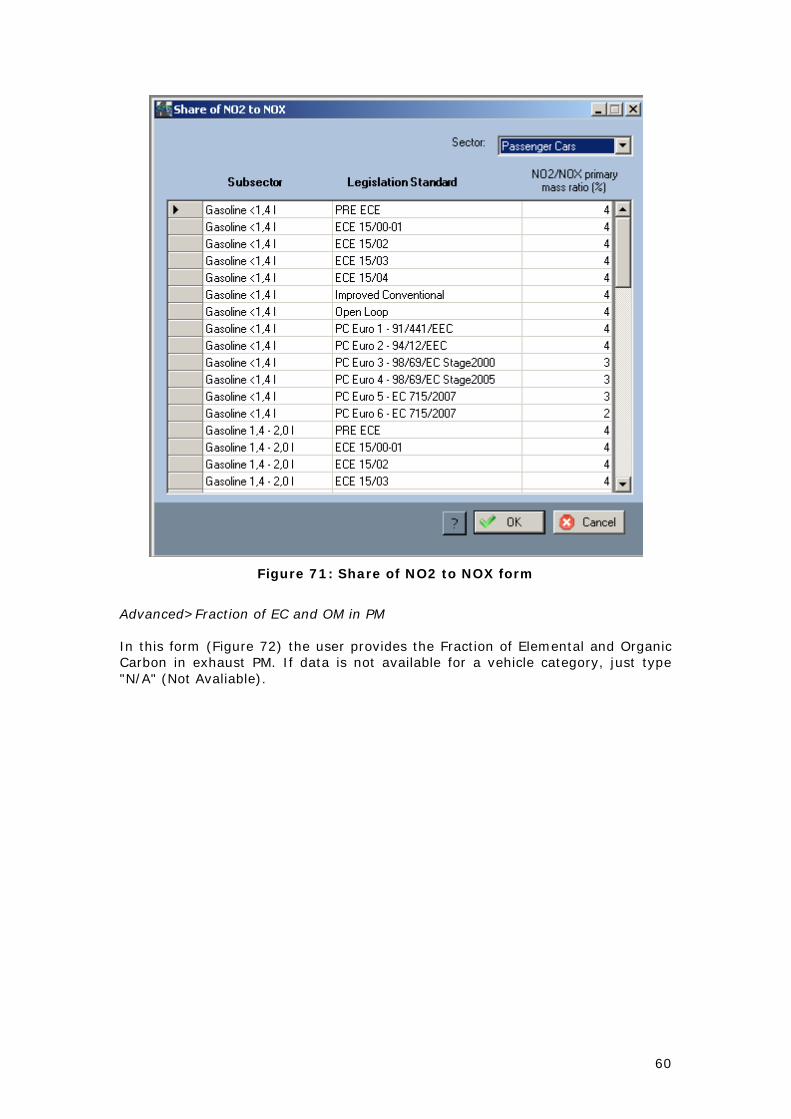
Advanced>Share of NO2 to NOX In this form (Figure 71) the user provides the share of NO2 to NOX via the NO2/NOX primary mass ratio. If data is not available for a vehicle category, just type "N/A" (Not Avaliable).

60

Figure 71: Share of NO2 to NOX form

Advanced>Fraction of EC and OM in PM In this form (Figure 72) the user provides the Fraction of Elemental and Organic Carbon in exhaust PM. If data is not available for a vehicle category, just type "N/A" (Not Avaliable).

61

Figure 72: Fraction of EC and OM in PM

Advanced>Parameters Under this menu (Figure 73) the user can view and alter parameters that are used for the calculation of the emission factors which are under the Calculation Factors menu. The available options are: Hot Emission Factors Parameters, Cold Emission Factors Parameters, Mileage Degradation Parameters and β-parameter reduction factor (bc).

Figure 73: Parameters menu

Advanced>Parameters>Hot Emission Factors Parameters With this form (Figure 74) the user can view and alter the hot emission parameters that are used for the calculation of the hot emission factors in the Calculation Factors>Hot Emission Factors form.

62

The user can view the parameters for each pollutant through the Pollutant drop-down list and for each sector through the Sector drop-down list. Use the Urban, Rural and Highway Mode tabs in order to view the corresponding parameters. Each mode also can have up to 3 speed ranges. View the different speed ranges' parameters by selecting the Speed Range radio buttons. One can also add a speed range for a specific combination of vehicle, pollutant and mode. Select the desired vehicle, and press Add Range, and a new speed range will be created for the selected vehicle. Likewise one can delete a speed range by pressing the Delete Range button. With the Formula button one can view the equation that is used in order to calculate the hot emission factors of the selected vehicle.

Figure 74: Hot Emission Factors Parameters form

Advanced>Parameters>Cold Emission Factors Parameters With this form (Figure 75) the user can view and alter the cold emission parameters that are used for the calculation of the cold emission factors in the Calculation Factors>Cold Emission Factors form. The user can view the parameters for each pollutant through the Pollutant drop-down list and for each sector through the Sector drop-down list. Use the month tabs in order to view the corresponding parameters. Each month also has up to 3 speed ranges. View the different speed ranges' parameters by selecting the Speed Range radio buttons. One can also add a speed range for a specific combination of vehicle, pollutant and month. Select the desired vehicle, and press Add Range, and a new speed range will be created for the selected vehicle. Likewise one can delete a speed range by pressing the Delete Range button. With the Apply Changes to all Months button one can apply the changes made to a specific vehicle for a month, to the rest of the months.

63

Figure 75: Cold Emission Factors Parameters form

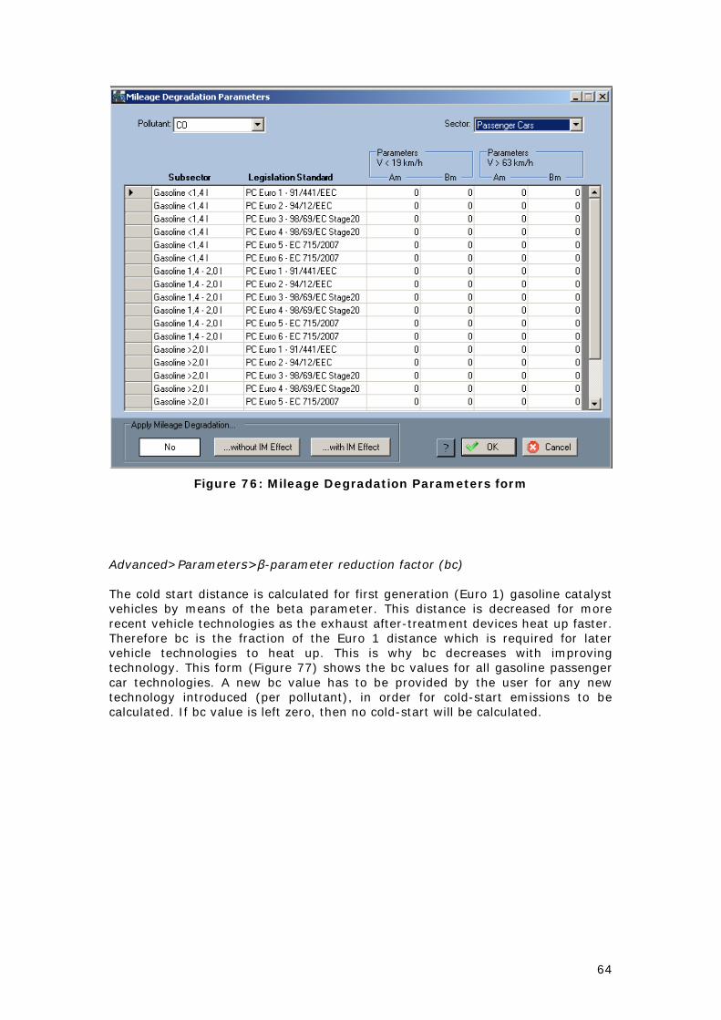
Advanced>Parameters>Mileage Degradation Parameters With this form (Figure 76) the user can view and alter the mileage degradation parameters that are used for the calculation of the mileage degradation factors in the Calculation Factors>Mileage Degradation form. The user can view the parameters for each pollutant through the Pollutant drop-down list and for each sector through the Sector drop-down list. The user may select between three options on the bottom of the form: No: No degradation factors are calculated and therefore no correction of the baseline hot emission factors is introduced. …without IM effect: If this option is selected then the degradation factors are calculated assuming that the applicable Inspection and Maintenance scheme is similar to Directive 92/55/EEC. …with IM effect: In this case, degradation factors are calculated assuming that an improved Inspection and Maintenance scheme is in place. By pressing one of the above buttons the Am and Bm parameters are automatically filled with the corresponding values. One can also provide his own values. For more details about the IM effect you may refer to the methodology report.

64

Figure 76: Mileage Degradation Parameters form

Advanced>Parameters>β-parameter reduction factor (bc) The cold start distance is calculated for first generation (Euro 1) gasoline catalyst vehicles by means of the beta parameter. This distance is decreased for more recent vehicle technologies as the exhaust after-treatment devices heat up faster. Therefore bc is the fraction of the Euro 1 distance which is required for later vehicle technologies to heat up. This is why bc decreases with improving technology. This form (Figure 77) shows the bc values for all gasoline passenger car technologies. A new bc value has to be provided by the user for any new technology introduced (per pollutant), in order for cold-start emissions to be calculated. If bc value is left zero, then no cold-start will be calculated.

65

Figure 77: β-parameter reduction factor (bc) form

66

5.1.8 Help Under this menu (Figure 78) the user can view some quick start instructions on how to use the application, the COPERT 4 Help Topics and some information about the programme. The available options are: Register, Check for updates, Quick Start Instructions, COPERT 4 Help Topics and About COPERT 4.

Figure 78: Help menu

Help>Register In this form (Figure 79) the user can unlock all the features of COPERT 4, if the installation is still in Demo version. One can provide the Serial Number that he was provided by our website (http://www.emisia.com/copert/license.html) and press Register. Important Note: The user must have administration privileges in order to be able to complete the process.

Figure 79: Registration form

Help>Check for updates The user can check automatically if there is a new version of COPERT 4 available on the website of Emisia (http://www.emisia.com/copert/Download.html) with the 'Help > Check for updates' menu item (Figure 80, Figure 81).

http://www.emisia.com/copert/license.html


67

Figure 80: "Check for updates" menu item

Figure 81: "Check for updates" message

Help>Quick Start Instructions With this command an html file will automatically open with the Microsoft Internet Explorer browser. In this file the basic steps are listed so that someone can quickly make a complete run using the COPERT 4 programme. Help>COPERT 4 Help Topics With this command a Help programme starts (Figure 82) that gives instructions and information to the user, on how to use the COPERT 4 application. All the instructions are divided into chapters the same way the user manual does. At any time during the inventory process the user can press F1 or the "?" button to see the corresponding COPERT 4 Help Topic.

68

Figure 82: COPERT 4 Help Topics

Help>About COPERT 4 With this command a form will appear (Figure 83) that shows some information about the programme, such as the version and the participants that take part in the research and development of COPERT 4.

69

Figure 83: About COPERT 4 form

70

6 Contact In case you need assistance with installing and running the application, or if you want to report any question or misbehaviour of the programme, please contact: • Dimitrios Gkatzoflias, e-mail: [email protected], tel: +302310 473374 • Chariton Kouridis, e-mail: [email protected], tel: +302310 473374

• Giorgos Mellios, e-mail: [email protected], tel: +302310 473352 • Leonidas Ntziachristos, e-mail: [email protected], tel: +302310 996003 • Zissis Samaras, e-mail: [email protected], tel: +302310 996014

mailto:[email protected]


