computational studies on new chemical species in the gas

Computational studies on new chemical species in thegas-phase and the solid-state.

Dissertation for the degree of Doctor Philosophiae

Patryk Zaleski-Ejgierd

University of HelsinkiDepartment of Chemistry

Laboratory for Instruction in SwedishP.O. Box 55 (A.I. Virtasen Aukio 1)

FIN-00014 University of Helsinki, Finland

To be presented, with permission of the Faculty of Science, University of Helsinki, for publicdiscussion in Auditorium CK112, Exactum (Gustaf Hällströmin katu 2, Helsinki), September 9th,2009, at 2:00 pm.

Helsinki 2009

Supervised by

Prof. Pekka PyykköDepartment of Chemistry

University of Helsinki

Helsinki, Finland

Reviewed by

Prof. Hannu HäkkinenDepartments of Physics and Chemistry

Nanoscience Center

University of Jyväskylä

Jyväskylä, Finland

Prof. Peter SchwerdtfegerCentre for Theoretical Chemistry and Physics

New Zealand Institute for Advanced Study

Massey University

Auckland, New Zeland

ISBN 978-952-92-5917-5 (paperback)

ISBN 978-952-10-5674-1 (PDF)

http://ethesis.helsinki.�

Yliopistopaino Helsinki 2009

"The more you know, the harder it is to take decisive action. Once you becomeinformed, you start seeing complexities and shades of gray. You realize that nothing isas clear and simple as it �rst appears."

� Bill Watterson, Calvin & Hobbe

The research for this thesis has been carried out at the Laboratory for Instruction inSwedish, Department of Chemistry, University of Helsinki during the time from August2006 to September 2009.

All the presented work was conducted under the supervision of Professor PekkaPyykkö. I wish to express my thankfulness to Pekka for giving me the opportunityto work with him, for his time and professional scienti�c support. After the three yearsI can't recall him ever saying "No" to me � Pekka, I owe my gratitude to you and forthat I sincerely thank you.

I want to thank my co-authors: Mikko Hakala and Michael Patzschke. Working withyou was a pleasure. I also thank the reviewers of my thesis: Professor Hannu Häkkinenand Professor Peter Schwerdtfeger. You valuable comments certainly increased value ofmy thesis.

Much of this work would have been more di�cult without the encouragement andsupport from the rest of the people working at the Department of Chemistry. � DearMichiko Atsumi, Raija Eskelinen, Ying-Chan Lin, Susanne Lundberg, Anette RojanoRosales, Anneka Tuomola, Nina Siegfrids, Gustav Boije af Gennäs, Krister Henriksson,Jonas Jusélius, Olli Lehtonen, Sergio Losilla, Mikael Johansson, Jesús Muñiz, MichaelPatzschke, Janne Pesonen, Sebastian Riedel, Nino Runeberg, Michal Straka, Dage Sund-holm, Stefan Taubert, Juha Vaara, Tommy Vänskä, Bertel Westermark and Cong Wang� I hereby thank you all for the discussions ... and arguments, for your support, helpand the strength you gave, when I needed it most.

Michiko and Ying-Chan, I cordially thank you for your support and conversations wehad. They were very helpful and important to me and my future decisions.

Dage, I was always looking forward to your advices and constructive remarks con-cerning my research � Thank you.

Mikael and Michael, you were both here when I started, you are both here when I�nish, and you are both nice friends whom I enjoyed talking to � Thanks.

Sergio, many thanks for your Spanish attitude and your sense of humor. You alwaysknew how to cheer me up.

Cong, I regret we never had opportunity to work on the same project. I'm sure itwould have been very fruitful and interesting. � Cong, thank you for being a goodfriend!

Finally, I want to express my deepest gratitude to Anna Olszewska. Dear Ania, youshould be a co-author of this thesis. We both know I would have not �nished it withoutyou standing by me.

In addition to personal contributions, the Finnish Centre for Scienti�c Computing(CSC) is acknowledged for providing computational resources. The following institutionsare acknowledged for providing �nancial support:

• University of Helsinki

• Finnish Centre of Excellence in Computational Molecular Science

• Magnus Ehrnrooth Foundation

• Finnish Cultural Foundation

• Svenska Tekniska Vetenskapsakademien i Finland

• Alfred Kordelin Foundation (Gust. Komppa fund)

• Laskennallisen Kemian ja Molekyylispektroskopian Tutkijakoulu (LasKeMo)

� Patryk Zaleski-Ejgierd, Helsinki 07.08.09

Dla Ani

Abstract

There is intense activity in the area of theoretical chemistry of gold.1,2 It is nowpossible to predict new molecular species, and more recently, solids by combining rela-tivistic methodology with isoelectronic thinking.

In this thesis we predict a series of solid sheet-type crystals for Group-11 cyanides,MCN (M=Cu, Ag, Au), and Group-2 and 12 carbides MC2 (M=Be-Ba, Zn-Hg). Theidea of sheets is then extended to nanostrips which can be bent to nanorings. Thebending energies and deformation frequencies can be systematized by treating thesemolecules as an elastic bodies. In these species Au atoms act as an 'intermolecularglue'. Further suggested molecular species are the new uncongested aurocarbons, andthe neutral AunHgm clusters.

Many of the suggested species are expected to be stabilized by aurophilic interac-tions. We also estimate the MP2 basis-set limit of the aurophilicity for the modelcompounds [ClAuPH3]2 and [P(AuPH3)4]

+. Besides investigating the size of the basis-set applied, our research con�rms that the 19-VE TZVP+2f level, used a decade ago,already produced 74 % of the present aurophilic attraction energy for the [ClAuPH3]2dimer. Likewise we verify the preferred C4v structure for the [P(AuPH3)4]

+ cation atthe MP2 level. We also perform the �rst calculation on model aurophilic systems usingthe SCS-MP2 method and compare the results to high-accuracy CCSD(T) ones.

The recently obtained high-resolution microwave spectra onMCN molecules (M=Cu,Ag, Au) provide an excellent testing ground for quantum chemistry. MP2 or CCSD(T)calculations, correlating all 19 valence electrons of Au and including BSSE and SO cor-rections, are able to give bond lengths to 0.6 pm, or better. Our calculated vibrationalfrequencies are expected to be better than the currently available experimental esti-mates. Qualitative evidence for multiple Au-C bonding in triatomic AuCN is also found.

i

List of Publications

List of publications included in the thesis

I. Zaleski-Ejgierd, P.; Hakala, M. O.; Pyykkö P. "Comparison of chain versus sheetcrystal structures for the cyanidesMCN (M=Cu-Au) and dicarbidesMC2 (M=Be-Ba, Zn-Hg)", Phys. Rev. B 2007, 76, 094104.

II. Pyykkö P.; M. O. Hakala; and Zaleski-Ejgierd, P. "Gold as intermolecular glue: atheoretical study of nanostrips based on quinoline-type monomers", Phys. Chem.

Chem. Phys. 2007, 9, 3025.

III. Pyykkö P.; Zaleski-Ejgierd, P. "From nanostrips to nanorings: A comparison ofgold-glued polyauronaphthyridines with polyacenes", Phys. Chem. Chem. Phys.

2008, 10, 114.

IV. Pyykkö P.; Zaleski-Ejgierd, P. "Basis-set limit of the aurophilic attraction usingthe MP2 method. The examples of [ClAuPH3]2 dimer and [P(AuPH3)4]

+ ion",J. Chem. Phys. 2008, 128, 124309.

V. Zaleski-Ejgierd, P.; Patzschke M.; Pyykkö P. "Structure and bonding of the MCNmolecules, M=Cu, Ag, Au, Rg", J. Chem. Phys. 2008, 128, 224303.

VI. Zaleski-Ejgierd, P.; Pyykkö P. "AunHgm clusters: mercury aurides, gold amalgams,or van der Waals aggregates?", J. Phys. Chem. A 2009, Article ASAP, DOI:10.1021/jp810423j.

VII. Zaleski-Ejgierd, P.; Pyykkö P. "Bonding analysis for sterically uncongested, simpleaurocarbons CnAum", Can. J. Chem. 2009, 87, 798.

ii

Contents

Abstract i

List of Publications ii

List of Abbreviations v

1 Introduction 1

1.1 Historical background . . . . . . . . . . . . . . . . . . . . . . . . . . 1

2 Wave-Function Theory 3

2.1 The N -electron Schrödinger equation . . . . . . . . . . . . . . . . . . 32.1.1 The Hartree-Fock method . . . . . . . . . . . . . . . . . . . . 42.1.2 Limitations of the Hartree-Fock method . . . . . . . . . . . . . 6

2.2 Post-Hartree-Fock techniques . . . . . . . . . . . . . . . . . . . . . . 62.2.1 Møller-Plesset Perturbation Theory . . . . . . . . . . . . . . . 62.2.2 Con�guration Interaction . . . . . . . . . . . . . . . . . . . . 92.2.3 Coupled-Cluster . . . . . . . . . . . . . . . . . . . . . . . . . 102.2.4 Limitations of post-HF methods . . . . . . . . . . . . . . . . . 11

3 Density-Functional Theory 13

3.1 The Hohenberg-Kohn Theorem . . . . . . . . . . . . . . . . . . . . . 133.2 Exchange-Correlation functional . . . . . . . . . . . . . . . . . . . . . 14

3.2.1 Local-Density approximation . . . . . . . . . . . . . . . . . . . 153.2.2 GGA and meta-GGA approximations . . . . . . . . . . . . . . 153.2.3 Hybrid functionals . . . . . . . . . . . . . . . . . . . . . . . . 163.2.4 Double-hybrid functionals . . . . . . . . . . . . . . . . . . . . 17

3.3 Limitations of DFT . . . . . . . . . . . . . . . . . . . . . . . . . . . 17

4 Solid-state implementations 19

4.1 Bloch's theorem . . . . . . . . . . . . . . . . . . . . . . . . . . . . . 194.1.1 First Brillouin Zone . . . . . . . . . . . . . . . . . . . . . . . 204.1.2 k-points . . . . . . . . . . . . . . . . . . . . . . . . . . . . . 204.1.3 Sampling grids . . . . . . . . . . . . . . . . . . . . . . . . . . 224.1.4 Band Structure . . . . . . . . . . . . . . . . . . . . . . . . . . 224.1.5 Density of States . . . . . . . . . . . . . . . . . . . . . . . . . 22

iii

iv

5 Approximations and methods 235.1 Born-Oppenheimer approximation . . . . . . . . . . . . . . . . . . . . 235.2 Harmonic approximation . . . . . . . . . . . . . . . . . . . . . . . . . 245.3 Basis sets . . . . . . . . . . . . . . . . . . . . . . . . . . . . . . . . . 25

5.3.1 Basis functions . . . . . . . . . . . . . . . . . . . . . . . . . . 255.3.2 Basis set size . . . . . . . . . . . . . . . . . . . . . . . . . . . 265.3.3 Contraction schemes . . . . . . . . . . . . . . . . . . . . . . . 265.3.4 Split-valence basis sets . . . . . . . . . . . . . . . . . . . . . . 275.3.5 Correlation-consistent basis sets . . . . . . . . . . . . . . . . . 275.3.6 Plane-wave basis sets . . . . . . . . . . . . . . . . . . . . . . 28

5.4 Basis set incompleteness error . . . . . . . . . . . . . . . . . . . . . . 285.5 Basis set superposition error . . . . . . . . . . . . . . . . . . . . . . . 295.6 Pseudopotentials . . . . . . . . . . . . . . . . . . . . . . . . . . . . . 305.7 Resolution of Identity . . . . . . . . . . . . . . . . . . . . . . . . . . 30

6 The relativistic framework 336.1 Dirac equation . . . . . . . . . . . . . . . . . . . . . . . . . . . . . . 336.2 The wave-function . . . . . . . . . . . . . . . . . . . . . . . . . . . . 356.3 Regular approximation . . . . . . . . . . . . . . . . . . . . . . . . . . 366.4 Perturbative corrections . . . . . . . . . . . . . . . . . . . . . . . . . 366.5 Two-component methods . . . . . . . . . . . . . . . . . . . . . . . . 37

6.5.1 Foldy-Wouthuysen transformation . . . . . . . . . . . . . . . . 386.5.2 Douglas-Kroll transformation . . . . . . . . . . . . . . . . . . 396.5.3 Other Two-Component methods . . . . . . . . . . . . . . . . . 40

7 Software 41

8 Results and Conclusions 438.1 New species . . . . . . . . . . . . . . . . . . . . . . . . . . . . . . . 43

8.1.1 Cyanides: MCN vs M3C3N3 (M=Cu, Ag, Au) . . . . . . . . . 438.1.2 Carbides: MC2 vs M3C6 (M=Zn-Hg, Be-Ba) . . . . . . . . . 448.1.3 In�nite, singly and multiply bonded chains and strips . . . . . . 468.1.4 Finite, gold-glued nano-strips and nano-rings . . . . . . . . . . 498.1.5 Aurocarbons . . . . . . . . . . . . . . . . . . . . . . . . . . . 508.1.6 AunHgm clusters . . . . . . . . . . . . . . . . . . . . . . . . . 52

8.2 Molecules as elastic bodies . . . . . . . . . . . . . . . . . . . . . . . . 558.3 Basis-set limit of the aurophilic interactions at MP2 level . . . . . . . . 598.4 High-accuracy calculations of MCN, M=Cu-Au . . . . . . . . . . . . 64

References 68

List of Abbreviations

AO Atomic OrbitalBO Born-OppenheimerBODC Born-Oppenheimer Diagonal CorrectionCC Coupled-ClusterCI Con�guration InteractionCP Counterpoise CorrectionDCB Dirac-Coulomb-BreitDFT Density Functional TheoryDK Douglas-KrollDOS Density of StatesDZ Double ZetaFBZ First Brillouin ZoneLCAO Linear Combination of Atomic OrbitalsLHS Left-Hand SideLDA Local Density ApproximationLSDA Local Spin Density ApproximationGGA Generalized Gradient ApproximationHF Hartree-FockIOTC In�nite-Order Two-ComponentF-W Foldy-WouthuysenFBZ First Brillouin ZoneFORA First-Order Regular ApproximationGTO Gaussian Type OrbitalsMP2 Second-order Møller-PlessetPES Potential Energy SurfacePP Pseudo-PotentialPW Plane-WaveQZ Quadruple ZetaRI Resolution of the IdentitySCF Self-Consistent FieldSTO Slater Type OrbitalSV Split-ValenceTZ Triple Valence ZetaWFT Wave-Function TheoryZORA Zeroth-Order Regular ApproximationX2C Exact Two-Component

v

vi

bcc body-centered cubicfcc face-centered cubichex hexagonalcc correlation-consistentpGTO primitive GTOpSTO primitive STOsc simple cubicvdW van der Waals

Chapter 1

Introduction

1.1 Historical background

During the 19th century, various phenomena were observed that could not be ex-plained by classical physics, see Table 1.1. Planck showed in 1900 that the intensity ofblack-body radiation,

I(ν, T )dν =2hν3

c21

ehνkT − 1

dν (1.1)

decays for high energies, if hν/kT � 1. The electromagnetic radiation takes place asquanta, whose energy is ∆E = hν. On the other hand, these energy di�erences arisefrom discrete energy levels,

∆E = Ei − Ef . (1.2)

This is implicit in the spectral formulae of Balmer, Rydberg, etc., and was explicitlyintroduced by Bohr.

The energies of the bound states are quantized. They are determined as the eigen-values, Ei, of the di�erential equation

HΨi = EiΨi. (1.3)

Here H is the Hamiltonian (the operator corresponding to the total energy) and Ψi isthe wave function of state i of the physical system. For a single particle moving in apotential V we have,

H = T + V, (1.4)

and

T = − ~2

2m∇2. (1.5)

The origin (1.3) of the quantization was found independently by Heisenberg, Schrödingerand Dirac. For time-dependent problems the eigenvalue problem is de�ned as:

HΨi = i~∂

∂ tΨi. (1.6)

1

2 1.1. Historical background

Phenomenon Discovery Models

Spectral lines (1814) Fraunhofer Balmer, Rydberg, Bohr, SchrödingerCovalent-bonding ∼(1828) Berzelius Heitler-LondonBlack-body radiation (1862) Kircho� Wien, Rayleigh-Jeans, PlanckPhotoelectric e�ect (1902) von Lenard EinsteinCompton e�ect (1923) Compton

Table 1.1: Phenomena requiring quantum mechanics.

For relativistic particles with spin 12one keeps the equations (1.3) and (1.6) but re-

places the non-relativistic H (1.4) by the relativistic Dirac Hamiltonian HD, see Chapter6.

Many-electron problems can be approached using Wave-Function Theory (WFT,Chapter 2) or Density-Functional Theory (DFT, Chapter 3).

Chapter 2

Wave-Function Theory

2.1 The N-electron Schrödinger equation

Consider an N -electron system. The electronic Hamiltonian, expressed in atomicunits, is taken as

H =N∑i

hi +N∑i>j

hij (2.1)

where the operators hi and hij are de�ned as

hi = −1

2∇2i −

A∑a

Zaria, hij =

1

rij= Vij. (2.2)

A wave-function, Ψ, satisfying the antisymmetry requirements

Ψ(i, j) = −Ψ(j, i) (2.3)

for the exchange of electrons i and j, can be approximated by a Slater determinant

Ψ =1

N !12

∣∣∣∣∣∣∣∣ϕ1(1) ϕ2(1) . . . ϕN(1)ϕ1(2) ϕ2(2) . . . ϕN(2). . . . . . . . . . . .

ϕ1(N) ϕ2(N) . . . ϕN(N)

∣∣∣∣∣∣∣∣ . (2.4)

The electronic energy, Eel, can be calculated as the expectation value

Eel = 〈Ψ|H|Ψ〉 . (2.5)

For a closed-shell system this yields

Eel = 2

N/2∑i=1

hii +

N/2∑i=1

N/2∑j=1

(2Jij −Kij), (2.6)

3

4 2.1. The N -electron Schrödinger equation

where hii is the sum of average kinetic and potential energy of the electrostatic attractionbetween the nuclei and the electron i,

hii = 〈ϕi(1)| − 1

2∇2(1)−

A∑a

Zar1a|ϕi(1)〉 , (2.7)

the Coulomb integral

Jij = 〈ϕi(1)ϕj(2)| 1

r12

|ϕi(1)ϕj(2)〉 , (2.8)

describes the potential energy for the electrostatic repulsion between two electrons, andthe exchange integral

Kij = 〈ϕi(1)ϕj(2)| 1

r12

|ϕi(2)ϕj(1)〉 (2.9)

arises from the requirement that Ψ be antisymmetric with respect to the permutationof any two coordinates.

2.1.1 The Hartree-Fock method

In the �rst approximation, the exact wave-function of a given state can be approx-imated by a single Slater determinant. Since the energy expression (2.6) is stationarywith respect to small variations in the orbitals ϕ, the variational approach may be appliedto �nd the set of orbitals that minimizes the value of Eel. According to the variationaltheorem, the wave-function constructed from such orbitals is guaranteed to yield thelowest possible energy within the single-determinant picture and within a given set oforbitals.

The goal of the Hartree-Fock procedure is to minimize the total electronic energy byintroducing in�nitesimal changes to the initial orbitals

ϕi → ϕi + δϕi.

The minimization procedure typically employs Lagrange's method of undetermined mul-tipliers. The L[{ϕi}] functional is introduced. By following the variational requirementδL = 0, a set of N equations de�ning the optimal orbitals is obtained. The Hartree-Fockequations are given as

F (1)ϕi(1) = εiϕi(1), (2.10)

where the εi values act as the undetermined multipliers, and F (1) is the Fock operator

F (1) =

[−1

2∇(1)2 −

A∑a

Zar1a

]+

N/2∑j=1

(2Jj(1)−Kj(1)) . (2.11)

Here the Coulomb operator Jj(1) is given as

Jj(1) = 〈ϕj(2)| 1

r12

|ϕj(2)〉 , (2.12)

2.1. The N -electron Schrödinger equation 5

while the exchange operator Kj(1) is de�ned with respect to the orbital upon which itoperates

Kj(1)ϕi(1) =

[〈ϕj(2)| 1

r12

|ϕi(2)〉]ϕj(1). (2.13)

Let us now assume that each molecular orbital ϕi can be approximated by a linearcombination of M atomic orbitals (LCAO)

ϕi =M∑µ=1

cµiχµ, (2.14)

where the χµ stand for one-electron basis functions. The atomic orbitals (AO) aretypically located at the nuclei, and the cµi are the expansion coe�cients. Introducingthe LCAO to the Hartree-Fock equations results in a new set of equations, now de�nedin a �nite space, spanned by the basis functions χµ

F (1)M∑µ=1

cµiχµ = εi

M∑µ=1

cµiχµ. (2.15)

Multiplying (2.15) by χν and integrating over all space yields

M∑µ=1

cµi (Fνµ − εiSνµ) = 0 (2.16)

where Fνµ and Sνµ are the elements of the Fock and overlap matrixes respectively:

Fνµ = 〈χν |F (1) |χµ〉 , Sνµ = 〈χν |χµ〉 . (2.17)

For each value of ν there are M such equations. To obtain the nontrivial solution, theso-called secular determinant must be equal to zero

det (Fνµ − εiSνµ) = 0. (2.18)

The solutions εi, are the orbital energies. Each solution for an occupied orbital includesthe kinetic energy of the electron in a molecular orbital ϕi and the energies resultingfrom the interactions with the nuclei and the remaining N -1 electrons. For this reason,the Hartree-Fock method is referred to as a Mean-Field Theory.

In terms of the eigenvalues, the total calculated electronic energy is

Eel =

N/2∑i=1

2εi −N/2∑j=1

(2Jij −Kij)

. (2.19)

By adding the internuclear repulsion energy

EAB =∑a=1

∑b=a+1

ZaZbRab

, (2.20)

6 2.2. Post-Hartree-Fock techniques

one �nally obtains the expression for the total energy of an N -electron system

EHF = Eel + EAB. (2.21)

Due to the orbital dependence of the Fock operator, a solution may only be obtainediteratively. Typically one diagonalises a semiempirical Hamiltonian for an initial solution,and using the initial values of the basis set expansion coe�cients, cµi, one performssubsequent calculations. The resulting orbitals serve as an input for the next cycle.The calculations are performed until a chosen criteria for convergence are ful�lled. Inthat respect, the Hartree-Fock method is also known as the self-consistent-�eld (SCF)method.

2.1.2 Limitations of the Hartree-Fock method

The Hartree-Fock method is a serious simpli�cation of the exact solution. The theoryis constructed in such a way, that the wave-function is antisymmetric with respectto the exchange of two electron positions. As such, the single-determinant Hartree-Fock wave-function, ΨHF , satis�es only the obligatory, formal requirements of a non-relativistic fermionic wave-function. Unfortunately, a single-determinant representationis insu�cient for an accurate, quantitative description of most chemical systems. Themain drawback of the HF method, is that it does not, by de�nition, include Coulombelectron correlation e�ects.∗ For certain cases, such as the aurophilic attraction studiedin this thesis, neglecting correlation e�ects leads to intermolecular repulsion insteadof attraction. Nonetheless, even for such di�cult cases, the HF method is a usefulbenchmark and a common starting approximation for more advanced, post-Hartree-Fock methods.

2.2 Post-Hartree-Fock techniques

The Hartree-Fock method has the intrinsic limitation of referring to a single-deter-minant wave-function Ansatz 2.4. To improve such a wave-function, a perturbativetreatment may be applied or the variational principle may be extended to more than onedeterminant.

2.2.1 Møller-Plesset Perturbation Theory

The Møller-Plesset perturbation theory3,4 is derived by splitting the usual electronicHamiltonian, H, into the sum of an unperturbed Hamiltonian, H0, and a perturbationoperator λV :

H = H0 + λV, (2.22)

∗only the Fermi correlation due to exchange is included in HF theory

2.2. Post-Hartree-Fock techniques 7

where λ is a small, but otherwise arbitrary perturbation parameter, and H0 is the N -electron Fock operator:

H0 = F =N∑i=1

F (i) =N∑i=1

h(i) +

N/2∑j=1

[2Jj(i)−Kj(i)]

. (2.23)

The perturbation potential, V , is de�ned as

V = H −H0 = H − F, (2.24)

where F is the Fock operator.

In the Møller-Plesset perturbation theory the wave-function and the energy expressionare being expanded into a power series with respect to the parameter λ:

Ψ = Ψ(0) + λΨ(1) + . . .+ λiΨ(i) =n∑i=0

λiΨ(i) (2.25)

E = E(0) + λE(1) + . . .+ λiE(i) =n∑i=0

λiE(i) (2.26)

A simple substitution of equations (2.22), (2.25) and (2.26) into the Schrödinger equa-tion results in the perturbation equation

(H0 + λV )

(n∑i=0

λiΨ(i)

)=

(n∑i=0

λiE(i)

)(n∑i=0

λiΨ(i)

). (2.27)

Collecting terms with the same power of λ yields a set of n equations:

H0Ψ(0)k = E

(0)k Ψ

(0)k

H0Ψ(1)k + VΨ

(0)k = E

(0)k Ψ

(1)k + E

(1)k Ψ

(0)k ,

H0Ψ(2)k + VΨ

(1)k = E

(0)k Ψ

(2)k + E

(1)k Ψ

(1)k + E

(2)k Ψ

(0)k .

. . .

Multiplying the LHS by Ψ(0)k and integrating over the whole space yields the energy

expressions:

E(0)k =

⟨Ψ

(0)k |H0|Ψ(0)

k

⟩, (2.28)

E(1)k =

⟨Ψ

(0)k |V |Ψ

(0)k

⟩, (2.29)

E(2)k =

⟨Ψ

(0)k |V |Ψ

(1)k

⟩, (2.30)

E(3)k =

⟨Ψ

(0)k |V |Ψ

(2)k

⟩, (2.31)

etc. Adding E(0)k and E

(1)k together, reproduces the Hartree-Fock energy of unperturbed

state Ψ(0)k .


The perturbative corrections are introduced through the E(2)k and higher-order terms.

To calculate the �rst correction, E(2)k , also called the MP2 correction, one introduces

the expansion

Ψ(1)k =

∑i

c(1)i Ψ

(0)i , (2.32)

and by putting it into (2.30) one obtains

E(2)k =

1

4

∑ia

∑jb

|(ij||ab)|2

εi + εj − εa − εb= EMP2

k (2.33)

where ϕi and ϕj are the occupied orbitals and ϕa and ϕb are the virtual ones, and εi,εj, εa, and εb being the corresponding orbital energies.

Spin-Component-Scaled MP2

In case of the MP2 method, the corrections to the unperturbed ΨHF wave-functionare only of second-order. It represents a compromise between accuracy and computa-tional cost. Grimme et al. proposed a modi�cation of the MP2 method based on thefact that the correlation energy can be separated into contributions from electron pairswith the same- and the opposite-spin, SS and OS respectively.5 In standard MP2, bothcontributions are treated equally

EMP2c = EMP2,SS

c + EMP2,OSc , (2.34)

where EMP2c corresponds to (2.33). Griemme showed that a simple correction to (2.34)

leads to a signi�cant improvement even in cases where MP2 typically fails.6 The cor-rection is based on a di�erent scaling of the EMP2,SS

c and EMP2,OSc components. The

Spin-Component-Scaled MP2 (SCS-MP2) method is de�ned as:

ESCS−MP2c = aSSE

MP2,SSc + aOSE

MP2,OSc , (2.35)

where aSS and aOS are empirical scaling factors: aSS=1/3 and aOS=6/5.

According to Griemme, in the HF method the SS electron pairs are already correlated,while the OS pairs are not. Low-order MP2 perturbation theory is unable to correct thisde�ciency. Hence, the non-HF-correlated pair contributions (OS) are scaled-up, whilethe HF-correlated contributions (SS) are scaled-down in the SCS-MP2 approach. Thissimple modi�cation yields results close to the very accurate QCISD(T) ones.6

Spin-Opposite-Scaled MP2

Based on the success of SCS-MP2 method, Jung et al. suggested to neglect thesame-spin (SS) contributions completely. By introducing scaling coe�cients aSS=0and aOS=1.3 one de�nes the Spin-Opposite-Scaled MP2 (SOS-MP2) method. Theaccuracy of SOS-MP2 method is slightly lower than that of SCS-MP2 but still remainssigni�cantly better than that of standard MP2. The major advantage is that the SOS-MP2 method scales with the 4th power of the system size (SCS-MP2 scales with the5th power) and thus it is applicable to much larger molecules.


2.2.2 Con�guration Interaction

The Hartree-Fock SCF procedure recovers a major part of the total energy. The partof energy missing due to the electron-electron correlation, Ec, is nevertheless essentialfor accurate results. It can be recovered by introducing the Con�guration Interaction(CI) expansion. The CI method assumes that the exact N -electron wave-function canbe reproduced by a linear combination of Slater determinants

Ψ =∞∑k=0

ckDk. (2.36)

For practical reasons, the ΨCI is constructed based on the Hartree-Fock ground-statedeterminant, by adding determinants corresponding to the singly, doubly, up to N -foldexcited states

ΨCI = c0D0 +∑s=0

csDS +∑d=0

cdDD +∑t=0

ctDT + . . .+∑n=0

cnDN . (2.37)

Using the HF determinant as a reference is justi�ed by the fact that it is the best

possible single-determinant approximation to the exact N -electron wave-function. As aresult, the c0 coe�cient of CI expansion (2.37) is typically ∼= 1 and the determinant D0

corresponds directly to ΨHF .

Although Ecorr is only a very small fraction of the total energy (typically 1 %),a huge number of electronic con�gurations is required to recover it. The number ofcon�gurations included in the CI expansion depends on two factors: the number ofelectrons in the system, N , and the number of basis functions, M , used in the LCAOexpansion. The total number of determinants can be estimated as

Number of determinants ∼ M !

N !(M −N)!. (2.38)

Typically M >> N , and the resulting number is huge. For practical purposes, the CIexpansion has to be truncated. The challenging task is to obtain su�ciently accurateCI wave-function with as few expansion terms as possible. A typical approach wouldbe to systematically truncate the expansion after including single, double, triple, orhigher excitations from the reference HF state. The excitation refers to assigning anelectron to an unoccupied orbital, instead of an occupied one. Although truncating theexpansion signi�cantly lowers the computational cost, a large number of terms remainsto be computed and the applicability of the CI method is very limited.

In addition, limiting the CI space to a �nite number of determinants leads to a size-extensivity problem. The truncated CI methods (CISD, CISDT, etc.) do not perform welleither in systems of di�ering size. With increasing size of a molecule, the proportion ofthe electronic correlation energy contained within a �xed reference space decreases. Tocompensate for this loss, techniques such as the Davidson correction7 or the QuadraticCI8 (QCI) methods has been devised.

For small systems and reasonable basis-sets, the so-called Full-CI method, serves asimportant benchmark, providing the exact solution to the N -electron non-relativistic


Schrödinger equation (within a given basis-set).

Due to their limitations CI methods are being surpassed by the much superiorCoupled-Cluster approximation.

2.2.3 Coupled-Cluster

The most important advance over the CI method is known as the Coupled-ClusterProcedure (CC). It resolves the problem of electron-correlation in a non-variationalmanner. Similarly to the CI methods, the Hartree-Fock ground-state is convenientlychosen as the reference state. An exponential form of the excitation operator T acts onthe ΨHF yielding the Coupled-Cluster wave-function

eTΨHF = ΨCC (2.39)

The cluster operator T

T =N∑i=1

Ti = T1 + T2 + . . .+ TN , (2.40)

generates all the possible N -fold excitations. For instance, the 2-fold excitation operatoracting on the reference state Ψ0

T2Ψ0 =occ.∑i>j

virt.∑a>b

tabij Ψabij (2.41)

generates double excitations from the pairs of occupied states, ij, to the pairs of virtualstates ab. The expansion coe�cients, tabij , also known as the excitation amplitudes, aredetermined by solving the Coupled-Cluster equations.

For most problems Coupled-Cluster calculations lead to very accurate result, even forrelatively short expansions. To illustrate this advantage of CC one can write down theexplicit form of the ΨCCSD wave-function

ΨCCSD = e(T1+T2)Ψ0 = Ψ0 +occ.∑i

virt.∑a

taiΨai +

occ.∑i>j

virt.∑a>b

tabij Ψabij +

1

2

occ.∑ij

virt.∑ab

tai tbjΨ

abij +

1

2

occ.∑i>j

occ.∑k>l

virt.∑a>b

virt.∑c>d

tabij tcdklΨ

abcdijkl + . . . (2.42)

From the form of ΨCCSD in (2.42) it is obvious that apart from the single and doubleexcitations (hence the acronym CCSD), the higher-order excitations are also indirectlyincluded as the so-called disconnected-clusters, with their amplitudes determined by thelower-order excitations. In principle, the CCSD wave-function contains all the possibleexcitations though the presence of disconnected clusters. This feature of CC is alsoresponsible for the fact that an arbitrarily truncated CC expansion remains size-extensive.This advantageous e�ects arise from the exponential Ansatz of the CC wave-function.


CCSD(T), the golden standard

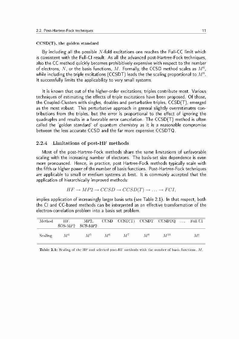
By including all the possible N -fold excitations one reaches the Full-CC limit whichis consistent with the Full-CI result. As all the advanced post-Hartree-Fock techniques,also the CC method quickly becomes prohibitively expensive with respect to the numberof electrons, N , or the basis functions, M . Formally, the CCSD method scales as M6,while including the triple excitations (CCSDT) leads the the scaling proportional toM8.It successfully limits the applicability to very small systems.

It is known that out of the higher-order excitations, triples contribute most. Varioustechniques of estimating the e�ects of triple excitations have been proposed. Of those,the Coupled-Clusters with singles, doubles and perturbative triples, CCSD(T), emergedas the most robust. This perturbative approach in general slightly overestimates con-tributions from the triples, but the error is proportional to the e�ect of ignoring thequadruples and results in a favorable error cancelation. The CCSD(T) method is oftencalled the 'golden standard' of quantum chemistry as it is a reasonable compromisebetween the less accurate CCSD and the far more expensive CCSDTQ.

2.2.4 Limitations of post-HF methods

Most of the post-Hartree-Fock methods share the same limitations of unfavorablescaling with the increasing number of electrons. The basis-set size dependence is evenmore pronounced. Hence, in practice, post Hartree-Fock methods typically scale withthe �fth or higher power of the number of basis functions. Post-Hartree-Fock techniquesare applicable to small or medium systems at best. It is commonly accepted that theapplication of hierarchically improved methods:

HF →MP2→ CCSD → CCSD(T )→ . . .→ FCI,

implies application of increasingly larger basis sets (see Table 2.1). In that respect, boththe CI and CC-based methods can be interpreted as an e�ective transformation of theelectron-correlation problem into a basis set problem.

Method HF, MP2, CCSD CCSD(T) CCSDT CCSDTQ . . . Full-CISOS-MP2 SCS-MP2

Scaling M4 M5 M6 M7 M8 M10 M !

Table 2.1: Scaling of the HF and selected post-HF methods with the number of basis functions, M .

Chapter 3

Density-Functional Theory

The wave-function of an N -electron system, Ψ, depends on 3N spatial and N spincoordinates. On contrary, the non-relativistic electronic Hamiltonian contains termsthat involve one- and two-electron integrals which involve up to six spatial coordinatesonly. As such, the wave-function contains more information than is actually needed. Analternative to Ψ, one that involves fewer variables, would thus be desired.

As it occurs, the energy of a system can be expressed in terms of �rst- and second-order spin-less density matrices. The problem was that there was no convenient pre-scription on how to calculate these matrices without referring to the wave-function in a�rst place. Currently, e�cient methods to resolve this problem are being developed.9

In 1964, Hohenberg and Kohn10 proved that the non-degenerate ground-state energy,wave-function and all the molecular properties are uniquely determined by the electronprobability density, ρ(r), which is the function of only three variables (r = x, y, z). Theground-state electronic energy, E0, can be de�ned as a functional of the electron densityρ(r):

E0 = E0 [ρ(r)] = E0[ρ] (3.1)

where the square bracket denotes a functional relation.

3.1 The Hohenberg-Kohn Theorem

The Hohenberg-Kohn theorem states that, if the non-degenerated ground-state elec-tron probability density ρ0 is known, then it is possible to calculate the ground-statemolecular properties from that ρ0.

Such an assumption implies that the wave-function is redundant and does not haveto be known. The theorem is a general statement and as such does not specify how theground-state energy E0 can be calculated. In fact, it does not even specify how can theprobability density itself be found.

In 1965 Kohn and Sham11 showed that the exact ground-state energy can be ex-pressed as

13

14 3.2. Exchange-Correlation functional

E0 = −1

2

∑i=1

⟨Ψi(1)|∇2|Ψi(1)

⟩−∑α

∫Zαρ(1)

r1αdv1+

1

2

∫ ∫ρ(1)ρ(2)

r12

dv1dv2+Exc[ρ],

(3.2)

where Ψi(1) denotes the Kohn-Sham orbitals and Exc[ρ] is the exchange-correlationfunctional. The notation Ψi(1) and ρ(1) indicate that the Ψi and ρ are taken asfunctions of the spatial coordinates of electron 1. Kohn and Sham showed that theexact ground-state electron density ρ0:

ρ0 =N∑i=1

|Ψi|2 , (3.3)

can be found from the Kohn-Sham orbitals. The orbitals itself are determined on thebasis of one-electron eigenvalue equations:

FKSΨi(1) = εi,KSΨi(1). (3.4)

Here the Kohn-Sham operator FKS is given as

FKS = −1

2∇2

1 −∑α

Zαr1α

+∑j=1

Jj(1) + Vxc(1), (3.5)

with the Coulomb operator Jj(1) de�ned as

Jj(1) =

∫|Ψj(2)|2 1

r12

dv2, (3.6)

and the exchange-correlation potential

Vxc =δ

δρExc[ρ]. (3.7)

The Kohn-Sham operator FKS is similar to the Fock operator (2.11). In the DFTformalism the exchange operators are replaced by Vxc, which handles the e�ects ofexchange and correlation simultaneously.

3.2 Exchange-Correlation functional

The DFT method is in principle an exact, yet it is impossible to solve the N -electronequations in exact manner. The problem resides in the exchange-correlation functional.Because the exact form of Exc[ρ] for molecules remains unknown, approximations haveto be introduced. As of this moment, scores of approximate functionals are available.

The hierarchy of density functional approximations is typically pictured as the so-called 'Jacob's ladder'. The quality of a functional is expected to increase as one getshigher up on the ladder. The �rst rung is the Local-Density Approximation (LDA), exactfor the uniform electron gas and often quite accurate for solids, particularly metals. The

3.2. Exchange-Correlation functional 15

second rung is the Generalized-Gradient Approximation (GGA), third is meta-GGA, etc.Nonetheless, at a given level of approximation it is di�cult to choose the best functionalwithout referring to previous calculations or experimental references. The systematicimprovement in accuracy is thus limited to factors such as the basis-set size.

3.2.1 Local-Density approximation

If ρ(r) varies slowly with position, the Exc[ρ(r)] may be expressed as:

Exc[ρ(r)] =

∫ρ(r)εxc[ρ(r)]dr (3.8)

where εxc[ρ(r)] is the exchange-correlation energy per electron for the homogeneouselectron gas with electron density ρ(r). The homogeneous electron gas is a hypotheticalin�nite-volume system consisting of an in�nite number of electrons. It is assumed thatthe distribution of electron density in such system is uniform and the number of electronsper unit volume has a non-zero value of ρ(r).

Applying the functional (3.8) yields the Local-Density Approximation (LDA). In amolecule the positive charge is localized at the nuclei, and the electron distributionvaries rapidly with the distance from a given nucleus. Molecular LDA calculations showonly fair agreement with experiment. Certain improvement is obtained by introducingdi�erent K-S orbitals, and thus densities, for electrons with di�erent spins. The extensionis called Local Spin-Density Approximation (LSDA).

The 'high-accuracy' LSDA calculations performed for selected diatomic molecules12

found average absolute errors of 2 pm in Re, 1.0 eV in De and 3.3 % in vibrational fre-quencies. While the distances are reproduced with reasonable accuracy, the dissociationenergies are poor. It is a typical behavior of LDA methods.

3.2.2 GGA and meta-GGA approximations

Since its introduction, the LDA was particularly popular in the �eld of solid-statephysics, but it was the generalized-gradient approximation (GGA) that made DFT pop-ular in quantum chemistry as well. The key improvement were improved binding energies.GGA expresses the exchange-correlation energy in terms of the densities, but also theirlocal gradients:

Exc[ρ(r)] =

∫ρ(r)εxc[ρ(r),∇ρ(r)]dr. (3.9)

The εxc[ρ(r),∇ρ(r)] is not uniquely de�ned for GGA resulting in many di�erent �avorsof GGA-based methods. Even more advanced are the so-called meta-GGA functions.These functionals include additional terms that depend on the Laplacian of the density.

Introduction of explicit gradient dependence improves the quality of DFT calculationsand yields better results for both solids and gas-phase species.

PBE functional

The PBE functional Perdew, Burke and Ernzerhof13 is constructed in such a way thatall the essential features of LDA are preserved. It combines them with the energetically

16 3.2. Exchange-Correlation functional

most important features of gradient-corrected nonlocality. The PBE functional in anon-empirical functional, whose all parameters are derived from theory.

3.2.3 Hybrid functionals

Hybrid functionals are a class of functionals where the exchange-correlation termincorporates a certain portion of exact exchange from Hartree-Fock theory. A hybridfunctional is usually constructed as a linear combination of the Hartree-Fock exact ex-change functional (EHF

x ) and several other exchange and correlation density functionals.The parameters determining the weight of each individual functional are speci�ed by �t-ting the results to reliable data. The concept of hybridizing the Hartree-Fock methodwith Density Functional Theory was �rst introduced in 1993 by Becke.

B3LYP functional

Among the many available hybrid functionals, the B3LYP exchange-correlation func-tional is the most popular among chemists. It is constructed in the following way:

EB3LYPxc = ELDA

xc + a0(EHFx − ELDA

x ) + ax(EGGAx − ELDA

x ) + ac(EGGAc − ELDA

c ),

where a0=0.20, ax=0.72, and ac=0.81 are three empirical parameters determined by�tting the predicted values to a set of experimentally known atomization energies, ion-ization potentials, proton a�nities, and total atomic energies. The EGGA

x and EGGAc

terms are based on the generalized gradient approximation: the Becke (B88) exchangefunctional14 and the correlation functional of Lee, Yang and Parr (LYP).15 The remainingELDAc is the Vosko, Wilk and Nusair (VWN) LDA functional.16

TPSS and TPSSh functionals

In 2008 Tao et al.17 proposed a new non-empirical meta-GGA exchange-correlationfunctional, TPSS. Construction of the functional is based on the Perdew-Kurth-Zupan-Blaha (PKZB) meta-GGA functional.18 As its predecessor the TPSS functional is de-signed to yield correct exchange and correlation energies through second-order in ∇ fora slowly-varying density (solids) and the correct correlation energy for any one-electrondensity (molecules).17

Initial tests17 show that the TPSS gives excellent results for a wide range of systems.In particular, it correctly describes bond lengths in molecules, hydrogen-bonded com-plexes and ionic solids. The practical advantage of TPSS functional is that it does notincorporate HF exchange. This feature is particularly important for solid-state calcula-tions where the exact HF exchange is usually inaccessible due to the exceedingly highcomputational cost.

Hybridizing the exact HF exchange with the non-empirical TPSS functional yields ahybrid. The TPSSh exchange-correlation functional is de�ned as

ETPSShxc = a0E

HFx + (1− a0)E

TPSSx + ETPSS

c

where the empirical parameter a0=0.10 is determined by minimizing the mean absolutedeviation in the enthalpy of formation of 223 molecules. The small value of a0 (smaller

3.3. Limitations of DFT 17

by about 20 % than for a typical hybrid functionals) indicates that the TPSSh functionalbetter approximate the still unknown exact exchange-correlation functional than otherstandard hybrid functionals.19

3.2.4 Double-hybrid functionals

An example on a new generation of the so-called double-hybrid functional is B2PLYP.The functional is constructed in such way that the explicit orbital correlation occurs.As a result, in addition to a non-local exchange contribution, a non-local perturbationcorrection for the correlation part is also introduced. The idea is rooted in the ab-initioKohn-Sham perturbation theory (KS-PT2) of Görling and Levy.20,21

First, one de�nes a standard hybrid-functional within the GGA approximation. Then,self-consistent Kohn-Sham calculations are performed. The resulting solutions, the KSorbitals and the eigenvalues, are used as input in the MP2-type calculations. Theresulting KS-PT2 correction replaces part of the semi-local GGA correlation. The non-local perturbation correction to the correlation contribution is given by

EKS−PT2c =

1

4

∑ia

∑jb

|(ij||ab)|2

εi + εj − εa − εb

The mixing is described by two empirical parameters ax and ac in the following manner:

EB2PLY Pxc = (1− ax)EGGA

x + axEHFx + (1− ac)EGGA

c + acEKS−PT2c (3.10)

where EGGAx and EGGA

c are the energies of a chosen exchange and correlation function-als, EHF

x is the exact Hartree-Fock exchange of the occupied Kohn-Sham orbitals, andEKS−PT2c is a perturbation correction term based on the KS orbitals.The method is self-consistent only with respect to the �rst three terms of (3.10).

For B2PLYP functional, the B88 exchange14 and LYP correlation15 are used with theparameters ax = 0.53 and ac = 0.27. According to Schwabe et al.22 the only knownbasic de�ciency of the B2PLYP approach is due to Self-Interaction Error (SIE). Thanksto the relatively large fraction of the SIE-free HF exchange, these a�ects are alleviated inB2PLYP. In addition, unwanted e�ects of increased Fock exchange, such as the reducedaccount of static correlation, are damped or eliminated by the KS-PT2 term.5

3.3 Limitations of DFT

Although most of the functionals are not de�ned in the strict ab-initio manner, theinclusion of a small portion of HF exchange and the e�cient empirical parameterizationyield surprisingly good results for many molecular properties. The results are oftencomparable with computationally much more expensive wave-function based methods,such as MP2 or even Coupled-Cluster methods. Nevertheless, most of the commonlyapplied exchange-correlation functionals share the same negative feature of not beingable to describe dispersion interactions in a reliable manner.23

18 3.3. Limitations of DFT

Chapter 4

Solid-state implementations

When dealing with solids, the question arises, how can one handle the in�nite num-ber of interacting electrons moving in the static �eld of an in�nite number of ions?What is the shape of wave-function that describes such system?

In a regular crystal, ions are arranged with regular periodicity. The potential V , feltby the electrons,

V (r) = V (r +R), (4.1)

is thus periodic. The periodicity can be employed to simplify the calculations. Bloch'stheorem exploits (4.1) to reduce the in�nite number of one-electron wave-functions tothe number of electrons in a unit cell.

Figure 4.1: The First Brillouin Zone of face-centered cubic (fcc) lattice with labels for high symmetrycritical points.

4.1 Bloch's theorem

Bloch's wave-function describes a particle moving in a periodic potential. It is de�nedas a product of two contributions, an exponential plane-wave envelope function and aperiodic function:

Ψn,k(r) = eikrΦn,k(r) (4.2)

19

20 4.1. Bloch's theorem

The Ψn,k product exhibits the same periodicity,

Ψn,k(r) = Ψn,k(r +R), (4.3)

as the potential. The corresponding one-particle energy En(k)=En(k + K) is alsoperiodic. The energy associated with index n varies continuously with wave-vector k.For that reason it is more appropriate to speak of energy bands n instead of discreteenergy levels.

According to Bloch's theorem all the distinct values of En(k) occur within the so-called First Brillouin Zone of the reciprocal lattice. The energy solutions, bands, areseparated in energy by a �nite spacing at each k. If the separation extends over allwave-vectors, it is called a band gap.

Within the independent electron approximation, all properties of a periodic systemcan be calculated from the band structure and the associated Bloch wave-function. Ap-plication of Bloch's theorem maps the problem of in�nite number of electrons onto theproblem of expressing the wave-function in terms of an in�nite number of reciprocalspace vectors within the FBZ. This problem is dealt with by sampling the Brillouin zoneat �nite sets of k-points.

4.1.1 First Brillouin Zone

Brillouin zones characterize crystal structures in momentum space.24 The First Bril-louin Zone (FBZ) is de�ned as the Wigner-Seitz cell in that reciprocal space. TheWigner-Seitz cell itself is de�ned as the smallest polyhedron enclosed by the perpendic-ular bisectors of the nearest neighbors to a lattice point. Higher-order Brillouin zonescan be de�ned as next-smallest polyhedra enclosed by bisecting planes.

For an extended periodic system, the uniquely de�ned FBZ is most important. Itcompletely characterizes the whole crystal. If one wants to consider all the possibleelectronic states in the in�nite crystal, one needs to investigate the FBZ only. Thisfollows directly from Bloch's theorem for the wave-function.

Within the First Brillouin Zone, points of high symmetry - called critical points ork-points - are particularly interesting (see Table 4.1). Of them, the Γ-point identi�esthe center of FBZ, while other points can identify for example ends of FBZ in di�erentdirections in k-space. Di�erent types of critical points can be de�ned for di�erent latticesymmetries. An example on face-centered cubic (fcc) lattice is shown in Fig. 4.1.

4.1.2 k-points

The First Brillouin Zone consists of a continuous set of k-points, throughout a regionof reciprocal space (k-space). The occupied states at each k-point contribute to theelectronic potential of bulk solid. There exist an in�nite number of k-points at whichthe wave-functions must be calculated. Those k-points that are very close together arealmost identical. It is thus possible to represent the electronic wave-functions over asmall region of reciprocal space at just a single k-point. This approximation allows theelectronic potential to be calculated at a �nite grid of points and yield the total energy

4.1. Bloch's theorem 21

Symbol Description

Γ Center of the Brillouin zone

Simple cubic (sc)M Center of an edgeR Corner pointX Center of a face

Face-centered cubic (fcc)K Middle of an edge joining two hexagonal facesL Center of a hexagonal faceU Middle of an edge joining a hexagonal and a square faceW Corner pointX Center of a square face

Body-centered cubic (bcc)H Corner point joining four edgesN Center of a faceP Corner point joining three edges

Hexagonal (hex)A Center of a hexagonal faceH Corner pointK Middle of an edge joining two rectangular facesL Middle of an edge joining a hexagonal and a rectangular faceM Center of a rectangular face

Table 4.1: Labeling of the most important First Brillouin Zone critical points for selected lattice sym-metries. For the fcc example, see Figure 4.1

of a solid. The error due the k-space sampling can be made arbitrarily small by choosinga su�ciently dense set of k-points.

The number of k-points necessary for a reliable calculation depends on the ex-pected accuracy and on the nature of the system. Metallic systems require an order-of-magnitude more k-points than semiconductors and insulators. Also, di�erent methodsconverge with di�erent speeds, which are highly dependent on the extent of the sampledk-space.

Typically the error due to the insu�cient number of k-point considered is not trans-ferable to di�erent lattice types (fcc, bcc, etc.) or with respect to the size of a unit cell.For small cells it is necessary to include more k-points while for large super-cells alreadythe Γ-point corresponds to many k-points in the First Brillouin Zone. Therefore the ab-solute convergence with respect to the number of k-points must be studied individuallyfor each case.

By sampling the electronic wave-functions at specially designed sets of k-points,very accurate approximations to the electronic potential can be obtained. The twomost common methods are those of Chadi and Cohen,25 and Monkhorst and Pack.26

22 4.1. Bloch's theorem

4.1.3 Sampling grids

In practical solid-state calculations one needs to use a �nite number of k-points tosample the FBZ. Choosing a �nite grid is acceptable as long as the orbitals vary smoothlywith k. In most of the cases a grid of Monkhorst and Pack26 is applied, particularlybecause it is unbiased by the choice of the k-points in the FBZ.

Monkhorst-Pack grid is a rectangular grid, spaced evenly throughout the FBZ. Sim-ilarly to the cut-o� energy, the choice of the grid size depends on the system. Theappropriate size is typically established by means of a convergence test. A general rulestates that the larger the dimensions of the grid, the �ner and more accurate will be thesampling.

4.1.4 Band Structure

Solving the Kohn-Sham equations yields N2orbitals for each of the k-points used in

sampling the FBZ. The resulting KS orbitals are solutions of a single-particle Schrödinger-like equation with the local Kohn-Sham potential. Using these solutions one can solvethe equations for k-points other than those in the original k-point set. Such completeset of eigenvalues for each k-point forms the band structure. In many cases it is agood approximation to the true band structure of the interacting system.

4.1.5 Density of States

The Density of States (DOS) describes the number of states that can be occupiedin a given system at each energy level. The zero value of DOS means that no statescan be occupied at the corresponding energy level. The product of the DOS and theprobability distribution gives the number of occupied states at a given energy perunit volume. The DOS analysis provides important information on physical propertiesof solids, such as conductivity and its type.

Chapter 5

Approximations and methods

5.1 Born-Oppenheimer approximation

In a system composed of electrons and atomic nuclei, the momentum transfer be-tween interacting particles is typically very small, due to a large di�erence in masses.Assuming that the forces acting on the particles are comparable and that their momentaare similar, the nuclear velocities must be much smaller than the velocities of electrons.Therefore it is not unreasonable to separate the electronic and nuclear motion. Such anapproach is called the Born-Oppenheimer (BO) approximation.27

By applying the Born-Oppenheimer approximation, the electronic eigenvalue problemis solved for the potential of nuclei at �xed locations. Once the ground state electroniccon�guration is known, the nuclear degrees of freedom could also be solved giving riseto nuclear motion. Varying the nuclear positions maps out the potential energy surface(PES) of the ground state.

The typical errors due to the Born-Oppenheimer approximation are small for theelectronic ground state and only slightly larger for excited states. The errors are usu-ally much smaller than those resulting from most other approximations used to solvethe N -electron Schrödinger equation (i.e. approximate treatment of electronic correla-tion, relativistic e�ects, basis sets, etc.). Hence the separation of nuclear and electronicvariables leads to a signi�cant reduction in computational cost. Had it not been for Born-Oppenheimer approximation, computational quantum chemistry might not be there inits current form. For small systems, calculations are now reported that treat electronicand nuclear motion on equal footing.28,29

Born-Oppenheimer Diagonal Correction: In a perturbative analysis of the BOapproximation, the �rst-order correction to the electronic energy due to the nuclearmotion is the Born-Oppenheimer diagonal correction (BODC):

EBODC = 〈Ψ(r;R)|TN |Ψ(r;R)〉 (5.1)

where Ψ(r, R) is an arbitrary electronic state and TN is the kinetic energy operator ofthe nuclei. Valeev and Sherrill estimated the BODC and its convergence toward theab-initio limit using CI wave-functions. They found that although the absolute valueis actually di�cult to converge with respect to the basis-set size, it is actually properlyestimated already at the Hartree-Fock level of theory.30

23

24 5.2. Harmonic approximation

5.2 Harmonic approximation

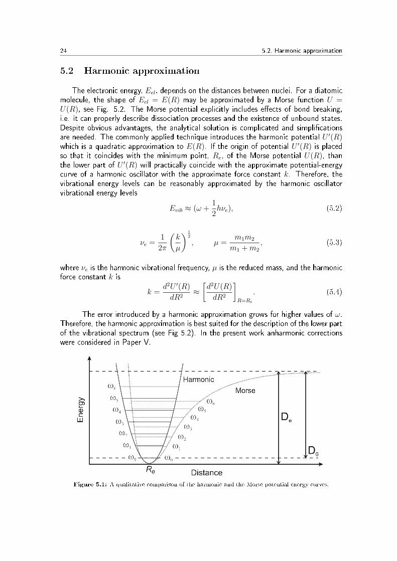
The electronic energy, Eel, depends on the distances between nuclei. For a diatomicmolecule, the shape of Eel = E(R) may be approximated by a Morse function U =U(R), see Fig. 5.2. The Morse potential explicitly includes e�ects of bond breaking,i.e. it can properly describe dissociation processes and the existence of unbound states.Despite obvious advantages, the analytical solution is complicated and simpli�cationsare needed. The commonly applied technique introduces the harmonic potential U ′(R)which is a quadratic approximation to E(R). If the origin of potential U ′(R) is placedso that it coincides with the minimum point, Re, of the Morse potential U(R), thanthe lower part of U ′(R) will practically coincide with the approximate potential-energycurve of a harmonic oscillator with the approximate force constant k. Therefore, thevibrational energy levels can be reasonably approximated by the harmonic oscillatorvibrational energy levels

Evib ≈ (ω +1

2hνe), (5.2)

νe =1

2π

(k

µ

) 12

, µ =m1m2

m1 +m2

, (5.3)

where νe is the harmonic vibrational frequency, µ is the reduced mass, and the harmonicforce constant k is

k =d2U ′(R)

dR2≈[d2U(R)

dR2

]R=Re

. (5.4)

The error introduced by a harmonic approximation grows for higher values of ω.Therefore, the harmonic approximation is best suited for the description of the lower partof the vibrational spectrum (see Fig 5.2). In the present work anharmonic correctionswere considered in Paper V.

Figure 5.1: A qualitative comparison of the harmonic and the Morse potential energy curves.

5.3. Basis sets 25

5.3 Basis sets

Most quantum chemical calculations are performed within a �nite set of M basisfunctions. The one-electron wave-functions are expanded as linear combinations of thosebasis functions

Ψ =M<∞∑i

ciχi → [c1, c2, ..., cM ]. (5.5)

One typically has to choose between more complete, and therefore computationallymore expensive basis sets, and smaller, less accurate but cheaper basis sets. If the basiswere expanded towards a complete set, the calculations would approach the exact result.In reality, a balance has to be found.

Di�erent molecular calculations typically require di�erent basis sets.

5.3.1 Basis functions

The �rst type of basis sets is constructed from Slater-type orbitals (STO). Thefunctional form of an STO is

χ ζ,n,l,m(r, θ, ϕ) = NYl,m(θ, ϕ)rn−1e−ζr. (5.6)

Here N is a normalization coe�cient and Yl,m(θ, ϕ) are spherical harmonic functions.

In general, the STOs are not solutions to the atomic Schrödinger equation. Howeverthe behavior near the nucleus and towards in�nity have the correct form. The radialpart lacks any nodal structure, but it can be recovered through linear combinations.Apart from the ADF code, Slater-type basis sets are typically used in high-accuracycalculations of atomic or diatomic systems only.

An alternative is provided by the Gaussian-type orbitals (GTO). The GTOs are de�nedas

χ ζ,n,l,m(r, θ, ϕ) = NYl,m(θ, ϕ)r2n−2−le−αr2

. (5.7)

The r2 in the exponent suggests that the GTO are inferior to the STOs. By de�nition,Gaussian-type functions lack the so-called cusp at the nucleus. At the nucleus, the �rstderivative is equal to zero, while in reality the derivative should approach a constant.More quantitatively, the Kato cusp condition states that

limr→0

⟨∂Ψ

∂r

⟩= −ZΨ(r = 0). (5.8)

As a result, the description of the wave function, close to the nucleus, provided by theGTO, is problematic. Moreover, the part further away from the nucleus is also describedinaccurately, because the GTO falls o� more rapidly as compared to the analogous STO.Both problems can be minimized to a high degree by introducing more basis functionsin the linear combination.

In principle, both Slater and Gaussian type basis functions can be used for the con-struction of a basis-set. Due to the nature of GTO, the number of required basis

26 5.3. Basis sets

functions is larger. A rough estimate indicates that approximately three times moreGTOs than STOs are needed to achieve a similar level of accuracy. Although GTOsare theoretically inferior to STOs, the much cheaper two-electron integrals make themcompetitive.

5.3.2 Basis set size

The simplest,minimal basis has only one e�ective Slater function per atomic orbital(such as 1s). Doubling the number of basis functions results in the Double-Zeta (DZ)basis set. In the case of hydrogen, such a set contains two s-functions with di�erentexponents. Increasing the number of basis functions provides �exibility and allows forbetter description of electron distribution.

In most chemical applications, a systematic increase (doubling, tripling, etc.) of thenumber of basis functions in the core and valence space does not provide equal increase inaccuracy, while it does increase the computational requirements. For instance, increasingthe number of functions with large exponents will improve the description of the coreregion, but it will have a minor e�ect on the valence space responsible for bonding.Since the energetically deep lying, or the core electrons, are essentially independent ofthe chemical environment, they can be accurately described with fewer basis functions.

5.3.3 Contraction schemes

The wave-function is not uniform. Di�erent parts of Ψ require di�erent treatment.The core electrons located close to the nucleus, account for much larger fraction of thetotal energy than the valence electrons. Variational optimization of a basis set withrespect to the total energy would favor the core electrons leaving the valence spacetoo poor in basis functions. For chemical purposes one would prefer the opposite. Toachieve this, typically one of the following contraction schemes is applied.

Segmented contraction: A set of M primitive Gaussian-type orbitals (pGTO) is�rst divided into subsets (s-, p-, d-, etc.). These secondary subsets are then contractedinto a set of gaussian type orbitals (cGTO) with predetermined coe�cients ci

χ1(cGTO) =b∑i=a

ciχi(pGTO),

In segmented contraction scheme, a given pGTO is usually used only once for each typeof cGTO.

General contraction: The basis set is not divided into secondary subsets. Insteadthe scheme allows for construction of contracted gaussian type orbitals (cGTO) usingall available primitives within the same angular momentum space. General contractionscheme provides additional �exibility but it is also computationally more expensive. Themost popular basis sets that rely on a general contraction scheme are the family ofcorrelation-consistent basis sets.

5.3. Basis sets 27

5.3.4 Split-valence basis sets

For an accurate bonding analysis, the valence space must be described particularlywell. In the split-valence (SV) basis set the functional space is divided into the coreand valence spaces. The doubling (tripling, etc.) of basis function applies to the valencespace only. Such an approach results in basis sets that are �exible enough for an accuratebonding description but remain computationally a�ordable even for larger sets.

Within the valence space, higher angular momentum functions are usually importantand must be eventually added to the basis set. For main-group elements a linear com-bination of s-, p- and d-functions is insu�cient for proper description. Introduction ofl-functions (l=f, g, h, etc.) provides additional degrees of freedom in the angular space.The f-function polarizes the d-function, just as the d-function polarizes the p-function.

For a single-determinant wave-function (i.e. ΨHF ), one set of polarization functionsis usually su�cient for the accurate description of charge polarization e�ects. For post-HF methods that treat electron correlation explicitly, the introduction of additional basisfunctions is essential. Electron correlation lowers the HF energy by letting the electronsavoid each other. Several distinct types of correlation can be identi�ed. In the case ofradial, 'in-out' correlation, one electron is much closer to the nucleus than the other.For proper description, additional basis functions with substantially di�erent exponentsare needed. In the case of angular correlation, electrons try to avoid each other byoccupying opposite sides of the nucleus. For this type of correlation, basis functionswith di�erent angular momenta are required. Both types of correlation are of the sameorder of magnitude.

Typically, exponents of polarizations functions are similar to the exponents of othervalence basis functions. It corresponds to the fact, that mainly the valence-electrons arecorrelated and the core-electrons are left unperturbed. For very accurate calculations,also core and core-valence polarization functions should be included.

5.3.5 Correlation-consistent basis sets

The correlation-consistent (cc) basis sets are a class of basis sets specially designedfor a systematic, high-accuracy recovery of the correlation energy. They include polariza-tion functions which contribute similar amounts of correlation energy at the same stage,independently of the type. For instance, if the p-space is correlated, the correlationenergy correction resulting from introducing the �rst d-function lowers the energy sig-ni�cantly. Introduction of an additional d-function will also lead to energy lowering, buta similar correction would result from introducing one f-function. Hence, both shouldbe included in the same step of basis set enlargement. In order to maintain consis-tent increase in quality, polarization functions are added in the order: 1d, 2d1f, 3d2f1g,4d3f2g1h, etc. To maintain a balance between the number of s- and p-functions andthe higher-angular-momentum polarization functions, the number of s- and p-functionsmust also increase in a consistent way.

A large number of correlation-consistent basis sets is available. The most commonare the cc-pVnZ (n = D, T, Q, 5, . . .). The acronym refers to 'correlation-consistentpolarized valence n zeta'. Several examples are illustrated in Table 5.1.

The scheme used in construction of cc basis sets leads to a rapid increase of the totalnumber of basis functions. This is particulary disadvantageous in wave-function based

28 5.4. Basis set incompleteness error

Basis s- and p-type pGTOs polarization pGTOs

cc-pVDZ 9s, 4p 1dcc-pVTZ 10s, 5p 2d, 1f,cc-pVQZ 12s, 6p 3d, 2f, 1gcc-pV5Z 14s, 9p 4d, 3f, 2g, 1hcc-pV6Z 16s, 10p 5d, 4f, 3g, 2h, 1i

Table 5.1: Selected correlation-consistent basis sets in terms of primitive gaussian type orbitals (pGTO).

theories, where the computation cost rises as Ma, a≥4 with respect to the number ofbasis functions.

5.3.6 Plane-wave basis sets

In addition to localized basis sets, plane-wave (PW) basis sets can also be used inquantum chemical simulations. Typically the number of plane-wave-functions is limitedby a cut-o� energy. Plane-wave basis sets are most suitable for calculations involvingperiodic boundary conditions. Certain integrals and operations are easier to implementand carry out.

An important advantage of any plane-wave basis is the systematic convergence to-wards the exact wave-function with respect to the cut-o� energy. All functions in thePW basis set are mutually orthogonal, and the basis set does not exhibit a basis setsuperposition error (see Section 5.5). However, when the volume of the cell changes,the number of plane-wave components varies discontinuously and corrections should beintroduced to compensate.31

Plane-waves are less well suited for gas-phase calculations. They are typically used,in combination with pseudopotentials (see Section 5.6), because they have di�cultiesdescribing the wiggles on the wave-function close to the nucleus.

5.4 Basis set incompleteness error

Typical calculations focus on the valence region of the wave-function. Most of thebasis sets are constructed in such way that the valence space is somewhat richer in basisfunctions, typically due to lower contraction. In the majority of cases, correlation of thevalence electrons is the most important. The core electrons are kept 'frozen', they arenot correlated.

The valence space of many modern basis sets can approach completeness and thecore-core and core-valence e�ects start to be non-negligible.32,33,34 Studies on refer-ence molecules shows that core-electron correlation e�ects should be considered uponenlarging the basis set to quintuple-zeta quality.35

Application of even larger, 6Z basis sets can still recover a minor fraction of thecorrelation energy, which for lighter elements is typically comparable to the magnitudeof relativistic e�ects.36 The rather uncommon 7Z and 8Z basis sets would lead toimprovement in correlation energy comparable in size to the error introduced by the

5.5. Basis set superposition error 29

Born-Oppenheimer approximation.For light elements, 6Z quality basis sets are typically large enough to reproduce the

non-relativistic limit. For calculations involving heavier elements other subtle e�ects,such as spin-orbit interactions, are typically as important as the basis sets size.

5.5 Basis set superposition error

Using a complete basis set is impossible. The number of basis functions must belimited to some �nite number, M , with some highest lmax.

Most calculations employ atom-centered bases with relatively few basis functions.Unfortunately, this technique is sensitive to the relative positions of nuclei. When com-paring two signi�cantly di�erent geometries, application of the nuclear-�xed basis setsleads to inconsistencies. For a given geometry the electron density around a nucleusA may be described by functions centered on nucleus B which was not present in thevicinity of A at the other geometry. In such situations, the �nite nature of the basis setmay considerably a�ect the calculations, particularly if weak interactions are involved.This e�ect is known as the basis-set superposition error (BSSE) and is a direct resultof the basis set incompleteness.

The BSSE vanishes only for a complete basis set. A brute-force solution to diminishthe BSSE is ruled out by the cost. In addition, adding a large number of basis functionscan also quickly lead to numerical issues such as basis set linear dependence.

The most-commonly applied approximate way of correcting for the BSSE is the coun-terpoise (CP) correction.

For a dimer, the uncorrected interaction energy, Eint, is calculated as

∆Eint = E(AB)∗ab − E(A)a − E(B)b (5.9)

where the monomers A and B are described with basis sets a and b, and the dimer ABis described by combined basis set ab. The asterisk indicates a dimer geometry. Toestimate how much of ∆Eint is due to the BSSE, four additional numbers are needed:a) the energies E(A)∗a and E(B)∗b of monomer A and B, with their corresponding basissets a and b, calculated at geometries they have in the dimer, b) the energies E(A)∗aband E(B)∗ab of both monomers at their dimer geometries, calculated with the combinedab basis set. The CP correction is then de�ned as

∆CP = E(A)∗ab + E(B)∗ab − E(A)∗a − E(B)∗b (5.10)

thus the CP-corrected interaction energy, ECPint is

ECPint = ∆Eint −∆CP . (5.11)

The counterpoise-corrected interaction energy typically approaches the basis set limitmuch faster than the uncorrected value.

30 5.7. Resolution of Identity

5.6 Pseudopotentials

Chemists are typically interested in the bonding which is determined by the valenceregion of the atoms. For light elements the core region includes few electrons and isusually of minor direct importance. On contrary, for heavy elements the core includedozens of electrons. The speeds of electrons moving in the vicinity of highly chargednuclei approach the speed of light. The relativistic e�ects are thus very pronounced.Although core electrons are not directly involved in bonding, changes in the deep-lyingorbitals a�ect the whole electronic structure.

Because the deep-core part of a heavy atom remains practically inert during anychemical reaction, the explicit treatment of the inner-most electrons can be reproducedby applying pseudopotentials.

The pseudopotential (PP) technique models the core-potential with a Gaussian ex-pansion

UPP (r) =∑i

airnie−αir

2

(5.12)

where parameters ai, ni and αi are determined by �tting to numerical data obtainedfrom high-precision all-electron calculations employing methods such as Multi ReferenceDirac-Hartree-Fock. This approach simultaneously eliminates large number of innerelectrons, and their basis functions from the calculations. In addition, pseudopotentialsemulate the relativistic e�ects at scalar or spin-orbit level at no additional cost.

Application of pseudopotentials �tted to the high-precision all-electron non-relativisticresults provides convenient insight into these two distinct realms.

Pseudopotentials: solids

Although plane-waves are the natural choice for basis functions for the periodiccalculations, they are poorly suited for describing the core-part of a wave-function. Alarge number of functions is typically needed to accurately describe the rapidly oscillatingelectronic wave-function close to the nucleus. In principle, it is possible to use Bloch'sfunctions with su�ciently high cut-o� energies to �nd the accurate solutions to theKohn-Sham equations for in�nite crystalline systems.

As in the case of discrete molecules, most physical and chemical properties of ex-tended systems depend mostly on the valence electrons. The pseudopotential techniquesare thus commonly applied. The pseudopotentials for solids are typically constructed insuch a way that they have no radial nodes in the core region of the wave-function. Thewave-function and the pseudopotential are identical to the all-electron wave-functionand potential outside a certain cut-o� radius. It signi�cantly lowers the computationalcost and allows for the inclusion of relativistic and other e�ects.

5.7 Resolution of Identity

To decrease the computational cost of calculations it is advantageous to separatethe Coulomb and exchange contributions to the total energy.

5.7. Resolution of Identity 31

One can expand the density ρ(r) in an auxiliary basis set

ρ(r) = ρ(r) =∑α

cαα(r), (5.13)

and introduce the Resolution of the Identity (RI)

〈ρ|ρ〉 ≥ 〈ρ|ρ〉 =∑α,β

〈ρ|α〉〈α|β〉−1 〈β|ρ〉 , (5.14)

where ∑α,β

|α〉〈α|β〉−1 〈β| ≈ 1. (5.15)

Using (5.15), an approximate form of the Coulomb operator (2.12), de�ned in theCoulomb metric37

〈x|y〉 =:

∫x(1)

1

r12

y(2)dτ

can be written as

J =1

2

∑α,β

〈ρ|α〉〈α|β〉−1 〈β|ρ〉 =∑

a,b,c,d,α,β

Dab 〈ab|α〉〈α|β〉−1 〈β|cd〉Dcd. (5.16)

The RI approximation is based on the expansion of products of virtual and occupiedorbitals in the auxiliary basis set. In (5.16), a four-center integral is replaced by three-and two-center integrals. Since such integrals are analytically solvable, the RI approxi-mation provides signi�cant computational savings with a minimal loss of accuracy. TheRI approximation for the Coulomb energy (RI-J) drastically decreases computationalcost of large-scale calculations, resulting in the asymptotic scaling proportional to N2.

32 5.7. Resolution of Identity

Chapter 6

The relativistic framework

In 1928 Dirac introduced a wave-equation that was consistent with both the principlesof quantum mechanics and the special relativistic requirement of Lorentz covariance

HDΨD = EDΨD (6.1)

Although equation (6.1) seems identical in form to the Schrödinger equation (1.3), itprovides signi�cant improvement in the description of a particles with spin s = 1

2.

6.1 Dirac equation

Dirac showed that in the absence of external electromagnetic �eld, the Hamiltoniandescribing an energy spectrum of a free electron is

HD = cααα · ppp+ βββm0c2 (6.2)

where m0 is the mass of electron in rest, ppp is the angular momentum operator, and cthe speed of light. Both ααα and ppp are vectors

ppp = (px, py, pz) ≡ (p1, p2, p3) ,

ααα = (αx, αy, αz) ≡ (α1, α2, α3) .

To satisfy E2 = m20c

4 + p2c2 for (6.2), the following relationships must hold

αiαj + αjαi = 2δij

αiβ + βαi = 0 (6.3)

β2 = 1 ,

where i, j = {1, 2, 3} and the Kronecker delta, δij, is de�ned using the Iverson bracketnotation as δij≡[i=j]. Such a de�nition implies that all the components of ααα and theβββ anticommute. They cannot be ordinary numbers. A possible representation satisfyingthe above anticommutation rules is a matrix representation. By de�ning an auxiliaryvector σσσ:

σσσ = (σx, σy, σz) ≡ (σ1, σ2, σ3) (6.4)

33

34 6.1. Dirac equation

constructed from the 2x2 Pauli matrixes

σσσx =

(0 11 0

)σσσy =

(0 −ıı 0

)σσσz =

(1 00 −1

), (6.5)

the ααα and βββ can be rewritten in a diagonal block-form

αααi =

(000 σσσiσσσi 000

)βββ =

(III 000000 −III

)(6.6)

where: III =

(1 00 1

)000 =

(0 00 0

). (6.7)

After applying the above relationships, the Dirac Hamiltonian, HD, is (in cartesiancoordinates)

HD =

p0 −m0c 0 −pz −(px + ipy)

0 p0 −m0c −(px + ipy) pz−pz −(px + ipy) p0 +m0c 0

−(px + ipy) pz 0 p0 +m0c

, (6.8)

with

p0 = − ~ic

∂

∂t. (6.9)

By inserting HD into the equation (6.1), and based on the matrix multiplicationrules, one concludes that the wave-function, ΨD, is a four-component vector.

An N-electron case

The Dirac equation (6.1) can be applied to N -electron problems. A central potentialis considered �rst. In the �rst approximation, an instantaneous Coulomb potential maybe introduced resulting in the N -electron Dirac-Coulomb equation(

N∑i=1

hD,i +N∑i<j

1

rij

)ΨD = EDΨD. (6.10)

Despite its successes, the Dirac-Coulomb equation (6.10) exhibits certain fundamentalproblems. Introduction of the r−1 Coulomb potential is a serious approximation basedon the non-relativistic assumption of instantaneous Coulomb interactions. In the rela-tivistic framework, the distance r between a pair of interacting bodies in not the onethat should be put into the potential. It reality, it should be a distance r′ between thetwo interacting bodies at the moment the interaction reaches the other partner. Theinteraction process is fast, it occurs with the speed of light, but it is not instantaneous.

6.2. The wave-function 35

This lack of delay in the Coulomb potential results in a small, but experimentally mea-surable e�ect.

A partial remedy came from Breit. Breit introduced an additional term to the po-tential for pair-interactions

Vij(r) = − 1

rij

[(αααi · rij) (αααj · rij)

r2ij

+αααi ·αααj]. (6.11)

Here the �rst term is the retardation term, it corrects for the interaction delay. Thesecond term, known as the Gaunt correction, is a �rst, magnetic, correction to theCoulomb repulsion term. The Gaunt term has a particularly considerable e�ect on theinner-core region of the wave-function where the electrons move fast.

Putting Breit's correction (6.11) to (6.10) results in theN -electron Dirac-Coulomb-Breitequation (

N∑i

hD,i +N∑i<j

1

rij−

N∑i<j

Vij(r)

)Ψ = EΨ. (6.12)

Both the retardation- and Gaunt-corrections are comparable in size but opposite in sign.Thus, they should always be considered simultaneously.

6.2 The wave-function

The four-component Dirac wave-function ΨD

ΨD =

ϕ1

ϕ2

ϕ3

ϕ4

, (6.13)

can be formally rewritten as a two-component vector

ΨD =

(φLφS

). (6.14)

where

φL =

(ϕ1

ϕ2

), φS =

(ϕ3

ϕ4

). (6.15)

The Hamiltonian (6.8) with external potential V , can also be written in the morecompact 2x2 form

HD =

(V +m0c

2 σσσpppcσσσpppc V −m0c

2

). (6.16)

Using relations (6.15) and (6.16), the four-component Dirac equation simpli�es to(V +m0c

2 σσσpppcσσσpppc V −m0c

2

)(φLφS

)= E

(φLφS

), (6.17)

36 6.4. Perturbative corrections

where the φL and φS are the large and small components of ΨD, respectively.

By re-writing the Dirac equation (6.17) explicitly

(V +m0c2)φL + σσσpppcφS = EφL

σσσpppcφL + (V −m0c2)φS = EφS

(6.18)

and using the second equation, the small component φS can be expressed in terms ofthe large component ΨL

φS =σσσpppc

(E − V +m0c2)φL. (6.19)

Eliminating the small component using relation (6.19), results in the two-componentDirac equation

(V +m0c2)φL + σσσpppc

1

(E − V +m0c2)σσσpppc φL = EφL, (6.20)

Equation (6.20) is fully equivalent to the four-component counterpart.

6.3 Regular approximation

The two-component Hamiltonian (6.16), written in a more convenient metric, is

HD = V +σσσpppc K−1 σσσpppc

2m0c2 − V. (6.21)

Through the expansion of (6.21) in a power series with respect to K

K =

(1 +

E

2m0c2 − V

), (6.22)

the regular approximation is formulated. The expansion is formally an exact two-component representation of Dirac equation de�ned as in�nite series. Already thezeroth-order term of the expansion introduces relativistic corrections to the non-relativisticlimit. The Zeroth-Order Regular Approximation (ZORA) has the advantage of beingvariationally stable even for the heaviest known elements (up to Z=137). Higher-orderapproximations can also be de�ned (FORA - First-Order RA, etc.) although they areless-commonly used due to the small e�ect they introduce.

6.4 Perturbative corrections

The Dirac-Coulomb-Breit Hamiltonian (6.12) can be treated in a perturbative man-ner. It can be decomposed into the partial energy operators, H i

DCB, with respect tothe parameter (Z

c)2. Several important advantages are: the resulting operators H i

DCB

are computationally easy to implement and have well-de�ned physical interpretations.

6.5. Two-component methods 37

The desired corrections can be added to the non-relativistic solutions in a very �exiblemanner. Within the �rst-order approximation:38

HIDCB =

∑i

p2i

2m0

+ V, V = −∑i

Ze2

ri+∑i

∑i>j

e2

rij(6.23)

is the non-relativistic N -electron Hamiltonian.

HIIDCB = − 1

8m30c

2

∑i

p4i (6.24)

describes the mass-velocity dependence.

HIIIDCB = −

∑j

∑i>j

e2

2m20c

2

[pi · pj

rij+

(rij · pi)(rij · pj)

r3ij

](6.25)

describes the 'orbit-orbit' interactions. It also partially accounts for retardation e�ects.

HIVDCB =

e~2m2

0c2

∑i

si ·

[(−∇iV )× pi +

∑j

∑j>i

2e

r3ij

(rij × pj)

](6.26)

is the 'spin-orbit' term. It describes the interaction between the orbital magnetic mo-ments resulting from the orbital motion of charge, and the spin magnetic moments.

HVDCB =

ie~4m2

0c2

∑i

[pi · (−∇iV )] (6.27)

is the Darwin term. It does not have a classical characteristic.

HV IDCB =

e2~2

m20c

2

∑i

∑i>j

{−8π

3(si · sj)δ3(rij) +

1

r3ij

[si · sj − 3

(si · rij)(sj · rij)

r2ij

]}(6.28)

is the 'spin-spin' interaction. The �rst term is the 'contact interaction', because it isnon-zero only when the particles are at the same position. The second term is theinteraction of the classical dipole-dipole type. Finally,

HV IIDCB =

e~m0c

∑i

[H(ri) · si +

e

m0cA(ri) · pi

](6.29)

is the interaction between spin and orbital magnetic moments with an external magnetic�eld H(ri).

6.5 Two-component methods

Attempt to solve the N -electron Dirac equation gives rise to solutions which aredi�cult to interpret. The existence of the continuum of negative energy eigenstates iscounterintuitive for a chemist's concept of a ground-state bound system. Attempts havethus been made to make the relativistic equations simpler and more comprehensible.

38 6.5. Two-component methods

6.5.1 Foldy-Wouthuysen transformation

The one-particle Dirac equation for a particle moving in the external �eld is

(cααα · πππ + βββm0c2 + eV )ΨD = EDΨD. (6.30)

In general, any Hamiltonian can be represented as a sum of the 'odd' and 'even' oper-ators, o and ε:

ε = 12(hD + βββhDβββ)

o = 12(hD − βββhDβββ).

(6.31)

If the commutation rules[βββ, o] = 0

[βββ, ε]+ = 0(6.32)

are satis�ed, ando = cααα · πππ, ε = eΦ (6.33)

then the 'odd' part of the Hamiltonian

(o+ βββmc2 + ε)ΨD = EDΨD (6.34)

can be eliminated up to an arbitrary power of (m0c2)−1.

Foldy and Wouthuysen applied a unitary transformation

UHDU−1UΨD = UEDU

−1UΨD. (6.35)

choosing the unitary operator U as

U = eiS =∞∑n=0

iS

n!, U−1 = e−iS = −

∞∑n=0

iS

n!(6.36)

where S = −iβ αp2m0c

. The third-order Hamiltonian becomes

H(3)D =

[πππ2

2m+m0c

2 − φ]− e

m0

sss ·BBB − ppp4

8m30c

2

+1

8m20c

2(∇∇∇ ·EEE)− 1

2m30c

2S · (EEE × ppp)− 1

2m30c

2(SSS ·BBB) π2. (6.37)

The resulting �ve-last terms can be used as �rst-order corrections to the non-relativisticresult.

The Foldy-Wouthuysen (F-W) transformation reduces coupling between the elec-tronic and positronic states. Unfortunately, decoupling of large and small componentsof ΨD a�ects also the operators. They are no longer variationally bound. Also, theF-W transformation can not be represented in closed form for a general potential, andcan only be approximated. Despite the �aws, the F-W transformation provides solutionswhich �t more comfortably into traditional concepts of electronic solutions. It also is agood starting point for more advanced considerations.

6.5. Two-component methods 39

6.5.2 Douglas-Kroll transformation

In 1974 Douglas, Kroll et al.39,40 presented a method of decoupling the large andsmall components of ΨD. The Douglas-Kroll (DK) method starts with the �rst-orderFoldy-Wouthuysen transformation, now performed in the momentum space. It is fol-lowed by a series of expansions in powers of the coupling strength parameter. The DKapproach yields operators that are bound and can be conveniently used in the variationalscheme.

The DK procedure starts from the unitary-transformation of the momentum-spacede�ned Dirac Hamiltonian

UHDU−1 = o+ βEp + ε = H ′D. (6.38)

The transformation splits the Hamiltonian into the odd and even contributions nowde�ned as

ε = Ap (Vx +RpVxRp)Ap

o = βAp [Rp, Vx](6.39)

where:

Ap =(Ep+m

2Ep

) 12, Rp = ααα·ppp

Ep+m0, Ep = (ppp2 +m2

0)12 . (6.40)

Next, using the anti-hermitian operator W1, a second unitary transformation, U ′1, isconducted

U ′1 =(1 +W 2

1

) 12 +W1. (6.41)

All coupling of the large and small component of the transformed wave-function areremoved up to the �rst-order in Vx. As suggested by Douglas and Kroll, separation toarbitrary orders in the external potential is possible by a consecutive application of theoperator

U ′n =(1 +W 2

n

) 12 +Wn. (6.42)

up to the n-th order.

For most chemical purposes, truncating the decoupling at the second-order is su�-cient. Higher-order contributions are typically important for the core electrons. Limitingthe decoupling does not substantially a�ect the description of the valence space. Thesecond-order Douglas-Kroll, one-particle Hamiltonian, H ′′DK , is

H ′′DK = Ep + ε1 +1

2

([Ep,W

21

]+

+W1EpW1

)(6.43)

The Hamiltonian (6.43) may be employed in conjunction with the Coulomb potentialto de�ne an N -electron second-order Douglas-Kroll (DK2) Hamiltonian

H ′′DK =N∑i=1

h′′DK,i +1

2

N∑i,j

1

rij(6.44)

A detailed investigations on heavy-atom-containing systems, proved the DK2 and higher-order DKn methods to be successful as compared to the fully relativistic results.41,42

40 6.5. Two-component methods

6.5.3 Other Two-Component methods

The free-particle F-W transformation is performed in a basis representation. TheDKH theory is nevertheless formulated as if it had been done at the operator level.Although formulation of the DKH transformation at operator level is possible, it makesit unnecessarily complicated, especially if higher orders are to be considered.

A �rst approximate quasi-relativistic theory, de�ned in a matrix form, was the so-called Normalized Elimination of the Small Component approximation of Dyall.43 Filatovand Cremer44 have cast the Regular Approximation into a matrix form, but the resultingequations were very lengthy even though they were only approximately correct.

In the context of the DKH approximation, the In�nite-Order Two-Component (IOTC)method of Barysz and Sadlej45 emerged as the �rst numerically exact, quasi-relativistictwo-component theory. The most impressive recent progress is of Kutzelnigg and Liu.46

They proposed a scheme that contains as special cases a surprisingly compact versionof In�nite-Order DKH as well as a very simple non-iterative method.

The idea of Kutzelnigg and Liu46 was to start from the representation of the Diracoperator in a �nite regular kinetically balanced basis. Then, a transformation is applied,that results in a quasi-relativistic Hamiltonian, expressed in the basis used for the uppercomponent of the Dirac operator. The eigenstates of the new quasi-relativistic Hamilto-nian are the same as those of the matrix representation of the Dirac Hamiltonian. Boththe matrix and the operator formulation of the so-called Exact Two-Component (X2C)method are equivalent. According to the authors, the X2C Hamiltonian is currently themost robust and accurate among the available relativistic methods.

Chapter 7

Software

A number of software packages is currently available. Some program packages tryto implement as many methods as possible, while other concentrate on a very speci�crange or even a single method. The results presented in this thesis were calculated usingthe following techniques and program packages:

MOLPRO: an extensive package of ab-initio programs for molecular electronic struc-ture calculations. The emphasis is put on highly accurate computations, with extensivetreatment of the electron correlation problem through multi reference CI, Coupled-Cluster and associated methods. Used here to calculate the Coupled-Cluster results.

TURBOMOLE: one of the fastest codes available for standard quantum chemicalapplications. Used here to calculate the HF/MP2 and DFT results, with and withoutthe aid of RI approximations.

ADF: one of the few STO-based programs. ADF can treat all elements of the periodictable. ADF is especially suited for transition metal compounds. It contains state-of-the-art relativistic methods including ZORA and spin-orbit coupling to properly treatheavy nuclei at the all-electron level. It provides a wide range of approximate relativis-tic Hamiltonians allowing for relativistic vs non-relativistic comparisons. Used here forcalculation of the spin-orbit e�ects.

Gaussian: designed for the needs of a user who does not necessarily possess anextensive theoretical background. With reasonable defaults for input data and the self-explanatory output it is probably the most intuitive and most widely used programpackage on the market. Used here for estimating anharmonic corrections to the vibra-tional frequencies.

VASP: An e�cient and reliable package for performing ab-initio quantum-mechanicalcalculations using ultra-soft pseudopotentials and a plane-wave basis set. The interac-tion between ions and electrons is described using Vanderbilt pseudopotentials or theprojector augmented wave method. Used as the main package for solid-state calcula-tions.

41

42 7. Software

Chapter 8

Results and Conclusions

8.1 New species

Quantum mechanics can be applied to calculate the properties of known molecules butit can also be successfully applied to inventing new species even before they are made.

8.1.1 Cyanides: MCN vs M3C3N3 (M=Cu, Ag, Au)

The solid Group-11 cyanidesMCN (M=Cu, Ag, Au) are well known. The experimen-tally determined structures correspond to hexagonally packed, in�nite -M -CN-M -CN-chains47 (see Fig. 8.1, A'). Following the study for Pyykkö et al.48 on a possible newsheet structure of solid AuCN (see Fig. 8.1, B'), we predicted that the AgCN and CuCNcould also have similar M3C3N3 sheet structures. This new structure contains triazine-type six rings of three carbon and three nitrogen atoms, C3N3, which are coupled toeach other by linearly coordinated metal atoms, forming a two-dimensional sheet struc-ture. The sheets attract each other weakly due to the metallophilic attraction. For the

Figure 8.1: The (A') chain structure ofMCN (P6mm), and the (B') sheet structure ofM3C3N3 (P62m).The spheres correspond to M , black circles to C and white circles to N atoms.

sheet structures, M3C3N3 (M=Au-Cu), local energy minima were found for the simplestacking geometry with symmetry P62m (see Fig. 8.1, B'). The total energies for thechain and sheet structures at 0K are compared in Table 8.1. For CuCN and AgCN theenergy di�erences are about 0.2 eV in favor of the chains. For AuCN there is practicallyno di�erence between the two structures, suggesting increased stability of the sheets.

43

44 8.1. New species

Case CuCN AuCN AuCN

3D sheet vs 3D chain -0.22 -0.18 0.002D sheet vs 1D chain -0.24 -0.21 0.03

Table 8.1: Total energy di�erence ∆E [eV] between the chain and sheet structures of Group-11 metalcyanides per MCN formula unit. A negative value indicates that the chain structure is energeticallypreferred.

8.1.2 Carbides: MC2 vs M3C6 (M=Zn-Hg, Be-Ba)

Following the valence-isoelectronic principle, the transition metal dicarbides, MC2

(M=Zn, Cd, Hg), and the alkaline-earth metal dicarbides, MC2 (M=Be, Mg, Ca, Sr,Ba), were studied.

Excluding BeC2, the remaining Group-2 dicarbides are experimentally known. Un-der normal conditions, MgC2 adopts the tetragonal P42/mmm symmetry, while theother carbides prefer the I4/mmm chain-like structure (see Fig. 8.2). For the knownGroup-2 dicarbides, the experimental structures were computationally reproduced andthe calculated covalent bond lengths are in good agreement with experiment [Paper I].

On contrary, no reference data is available for the Group-12 dicarbides. For theMC2

(M=Be, Zn-Hg), the three types of tetragonal packing presented in Fig. 8.2 were in-vestigated. In all the cases tetragonal I4/mmm symmetry (Fig. 8.2, B) was preferred.No additional chain-like local-minima were identi�ed.

Figure 8.2: Investigated crystal structures for chain-type metal dicarbides MC2 (M , spheres; C, blackcircles: (A) tetragonal P4/mmm, (B) tetragonal I4/mmm, and (C) tetragonal P42/mmm.

Isolated sheets: In the search of isolated, 2D M3C6 sheets, the previously identi�edhexagonal sheet-structure of cyanides was used as a starting point. Now, the six-membercarbon rings are coupled together from the corners by the metal atoms (see Fig. 8.3,left). The calculations in this geometry, with a large sheet-sheet separation, yieldedminimum energy structures for M=Be, Zn-Hg.

For the remaining metals, M=Ca-Ba, these 2D sheet spontaneously relaxed to aslightly di�erent, hexagonal geometry. The carbon rings rotated by 30o with respect tothe initial structure (see Fig. 8.3, right). In this new structure, metal atoms are located

8.1. New species 45

in the midpoint of the line connecting the C-C edges of every two benzene-like rings.

Figure 8.3: The two identi�ed local sheet-like local minima for M3C6 carbides. The lest geometry wasadopted by carbides with M=Be, Zn-Hg, while the right one by those with M=Ca-Ba.

Packed sheets: Considering 3D packing of the 2D sheet structures, a simplestacking analogous to cyanides was found purely repulsive for both nonrotated androtated cases (D) and (F), respectively. Instead, an alternative 3D packing had to beintroduced, with every second sheet translated by the vector v=(1

2a, 1

2a, 0) (see Fig.

8.4). For such systems, stable 3D geometries, (E) and (G), were found (Fig. 8.4).

Figure 8.4: Investigated crystal structures for sheet-type metal dicarbides M3C6 (M=Be-Ba, Zn-Hg).

The structural preference with respect to the total energy is summarized in Fig. 8.5.The energy di�erence ∆E is given for each dicarbide per MC2 unit. A negative valueindicates that the chain structure is preferred. For the experimentally known dicarbides,M=Mg-Ba, the chains are energetically more stable, as expected. The energy di�erenceroughly increases following Z, being in all the cases less than 1 eV. Interestingly, for theexperimentally unknown dicarbides, M=Be, Zn, Cd, and Hg, the sheet structure is pre-dicted to be more stable, and the energy di�erence likewise increases roughly following Z.

Electronic properties: Although DFT is known to underestimate band gaps, onecan clearly see the general trends between the geometries and between the elements.In the case of both cyanide and dicarbide chain structures, all the known and predicted

46 8.1. New species

Figure 8.5: Total energy di�erences ∆E [eV] between the most stable chain and sheet structures forGroup-2 and -12 metal dicarbides.

one-dimensional isolated and 3D structures are found to be insulators [Paper I]. For thepacked dicarbide chain structures, the band gap is largest for the HgC2 (3.7 eV) andsmallest for BaC2 (1.6 eV). The packed chain structures exhibit systematically smallerband gaps than the isolated chains due to the increased overlap of the valence orbitals.The only exception to this picture is BaC2. All the predicted chain dicarbides, MC2

(M=Zn-Hg), have larger gaps than the known dicarbides of Group-2.For both the cyanide and dicarbide isolated 2D sheets, the band gaps are clearly

smaller than for the chain structures. Furthermore, packing the sheets in a 3D structuresdecreases the band gap value even more.

For dicarbide sheets, we identify two candidates that appear metallic at the presentDFT/GGA level of theory: Sr3C6 and Ba3C6. Both systems may have a signi�cantamount of charge carriers. The rest of the cyanide and dicarbide compounds are foundto be either insulators or semimetals with a slight band overlap between the occupiedand unoccupied states.

8.1.3 In�nite, singly and multiply bonded chains and strips

A family of in�nite 'nano-chains' and doubly-, triply- and multiply-bonded strips ispredicted (Fig. 8.6). They consist of single, double or triple aromatic rings linkedtogether by strong C-Au-C, C-Au←N or N→Au←N bonds. Depending on the systemthese 1D nano-structures are found to be insulators, narrow- or zero-gap semiconductors,or metals. Varying the nitrogen content in the aromatic rings is found to have a minore�ect on the geometries.

The band structure of the 1D strips can be interpreted in a rigid-band picture. Theorbital character of the states at the Fermi level has been analyzed indicating, in certaincases, similarities with the band structure properties of graphene.

A large number of closed− shell species has been introduced and investigated (Fig.

8.1. New species 47

8.6). Many of the systems contain a closed-shell C-Au←N bond, although stable sys-tems can be found also for larger or smaller electron counts per bond. For instance, thepresent C-Au-C case is isoelectronic with the case where a coinage-metal cation bridgestwo N-heterocyclic carbenes with one extra conduction electron.49

Nano-chains: The simplest considered structures are the singly-bonded pyridine-based nano-chains (Fig. 8.6, 8a-8c). The calculated polymerization energy of 8b is1.65 eV per monomer. As for the two other cases, 8a and 8c, it is 0.3 and 0.2 eV,respectively. Those systems will enjoy nearly free rotation of the monomers about thepolymer axis. They would probably be much less sti� compared to the more complexstrips. The calculated polymerization energy emphasizes the strength of the C-Au←Nbond as compared to the C-Au-C and N→Au←N ones.

Double-ring nano-strips: The family of naphthalene-derived nano-strips 1a-1dis depicted in Fig. 8.6. The calculated Au-Au distance are in the range of 255-270 pm,falling between the values in Au2 dimer (247 pm) and bulk crystal (288 pm). The mainfeature in the �nal geometry of those strips is that the gold atoms protrude slightly frominitial position due to the electrostatic repulsion, resulting in the C-Au←N angle beingbent towards the strip edge.

Triple-ring nano-strips: Two types of anthracene-derived nano-strips are pro-posed. The �rst family is a straightforward analog of the double-ring structures, nowwith three bridging gold atoms (see Fig. 8.6, 2a-2e). The middle bond is linear. Thetwo lateral Au atoms are repelled by the central gold, leading to signi�cant bending ofthe corresponding bonds.

The second family (structures 3a-3e) is a modi�cation of cases 2a-2e. The centralAu atom is now replaced by a hydrogen. The expected e�ect was to relieve the Au-Aurepulsion. Indeed, as a consequence, the two lateral bonds return to linear positions.

For all the double- and triple-ring structures 1-3, the C-N, Au-C and Au-N distancesin the suggested new nano-strips are typical and similar with the distances calculated forAu3C3N3 and M3C6 systems [Paper I]. For all the nano-strips discussed, the monomergeometries are found to be planar.

Ladder-type nano-strips In this proposal, two in�nite poly-acenes are 'glued' byAu atoms. In the case of four structures, 4a-4d, the Au-Au distance is to small hencethe positively charged gold atoms strongly repel each other. Due to this unfavorableinteraction, the structures are no longer planar. With alternating Au atoms being now10-40 pm above and below the plane, the gold atoms form a zig-zag chain-structure.Nonetheless, even this kind of distortion does not prevent all four structures (4a-4d)from being unstable against vibrations. Only by replacing each second gold atom withhydrogen (see Fig. 8.6, 4e) the steric tension is minimized and the resulting strip doesnot exhibit any imaginary frequencies.

Electronic properties: We found that a modi�cation of the C/N content of thering changes the orbital character of the Density of States (DOS) relatively little froma qualitative point of view. Therefore, as a �rst approximation, the DOS is interpreted

48 8.1. New species

Figure 8.6: Series of proposed nano-chains and nano-strips.

in the rigid-band picture. In the C-rich cases, electrons are partially depleted from thesaturated 2pz, 5dyz and 6s orbitals, giving rise to a conduction band of a mixed character.Such systems could be thought of as having a 1D p-type band with contributions dueto the metal valence 5dyz and 6s electrons. In the N-rich cases, electrons are injectedinto the unoccupied 2pz states, resulting in a p∗-type conduction band. The additionof protective groups (Fig. 8.6, 5a, 5b) was found to have very little e�ect on the bandstructure. The orbital character of the bands at Ef remained similar.

In general, the behavior of the double- and triple-ring cases 1 and 2 is similar, withone notable di�erence. The all-carbon structure 1a is vibrationally unstable comparedto the similar all-carbon 2a case.

The ladder-type strips behave di�erently. Here, only the 4e system was found stableagainst vibrations. In this system gold again acts only as a 'glue'. It was found that

8.1. New species 49

the presence of the gold atoms does not strongly a�ect the electrical conductivity. TheDOS shows that this system is a zero-bandgap semiconductor, and the states aroundthe Fermi level have only pz character, originating from the C and N atoms only. Thesestates form a p-type valence and conduction bands. Those valence bands which have Auorbital character are particularly �at, suggesting negligible Au orbital interaction alongthe strip. Intriguingly, the conduction band of graphene is also formed from the 2pzorbitals and has zero-bandgap semiconductor properties. In graphene the p-band has nooverlap with the �lled valence bands (2s, 2px, 2py), whereas in proposed 4e the p-bandcrosses the d-bands as one moves o� the Γ-point.

8.1.4 Finite, gold-glued nano-strips and nano-rings

Gold atoms can act as an 'intermolecular glue', coupling (hetero)aromatic rings, typ-ically through C-Au←N bonds. An example on gold-glued poly(triaurotriazine) sheets,and in�nite nano-strips was already discussed. Although the sheets [Paper I] and the in-�nite nano-strips [Paper II] are yet experimentally unknown, the chemically stable dimersand oligomers of 2,6-diauro-1,5-naphthyridine molecule are known.50,51 We investigatedseveral such �nite nano-strips. We also propose to bend the strips to form 'gold-glued'naphthyridine-based cylindrical structures with n monomeric units (n=4-10).

Figure 8.7: The notation scheme for strips and rings.

Nano-strips: The simplest member of the strip family is the 2,6-diauro-1,5-naphthy-ridine molecule. Both the molecule, and the longer strips were optimized with C2h sym-metry (Fig. 8.7, left). The geometry optimization did not reveal any signi�cant bondlength alternation for longer strips. The vibrational analysis shows only real frequencies.Selected results are given in Table 8.3.

Length \ n 4 5 6 7 8 9 10

N3-Au 214.6 213.5 213.3 213.0 212.9 212.8 212.7C5-Au 200.6 200.4 200.4 200.4 200.4 200.4 200.4Au-Au 274.4 272.8 272.4 271.7 271.4 271.2 271.1

r 442.4 553.4 6.411 775.9 871.1 998.5 -

Table 8.2: Calculated bond lengths and radius, r, for polynaphthyridine rings. For the atom notation,see Fig. 8.7. All values in pm.

50 8.1. New species

n = 1 n = 2 n = 3 n = 4Length I I II I II III I II III IV

C3-Au 197.9 200.7 197.7 200.6 200.5 197.7 200.6 200.4 200.5 197.7

C8-Au 197.9 197.7 200.7 197.7 200.5 200.6 197.7 200.5 200.4 200.6

N5-Au - 212.8 - 212.7 212.8 - 212.7 212.6 212.8 -

N10-Au - - 212.8 - 212.8 212.7 - 212.8 212.6 212.7

n 1 2 3 4 5 6 7 8 9 10L 678.7 1376.6 1675.0 2772.9 3870.8 4968.7 6066.6 7164.5 8262.4 9360.3

Table 8.3: Selected bond lengths and strip lengths, L, tabulated for selected �at polynaphthyridinesystems (for the monomer notation and bond description, see Fig. 8.7).

Nano-rings: Six naphthyridine-based rings with the number of Au2C8N2H4 mono-meric units varying from 4 to 10 are predicted and investigated. All systems were relaxedwith �xed Dn symmetry (Fig. 8.7, right). Each ring can be viewed as n (hetero)aromaticmonomers 'glued' together by gold atoms. We did not observe any signi�cant alterna-tion between the rings with odd and even n. Interestingly, the N-Au and the Au-Au bondlengths decrease slightly for larger systems, while the Au-C distances remain practicallythe same. The qualitative bonding analysis indicates that the present (hetero)aromaticmonomers appear to be simply 'glued' together by gold atoms. The predicted rings couldalso exhibit interesting dispersion interactions with atoms or molecules inside them.

Mechanical properties: We found all the considered strip and ring structuresstable with respect to vibrations. To get additional feeling for the mechanical rigidity ofproposed rings we bent the �nite nano-strips to rings and compared that bending energywith the one for polyacene rings with similar dimensions. Apart from the energy neededto create the ring from a linear strip, we also used the in-plane deformation vibrationalfrequencies as a criterion for rigidity. The analysis is described in more detail in Section8.2.

8.1.5 Aurocarbons

Gold is noble, but its chemistry is fascinatingly rich. One of the interesting aspectsof gold chemistry is the analogy between Au and H. Recently Naumkin52 considered thepossibility of completely 'aurating' neopentane, C(CH3)4. Concerning the gas-phase,the dication CAu2

2+ was mass-spectroscopically observed by Gibson.53 Its electronicstructure was interpreted by Pyykkö et al.54 as [Au=C=Au]2+, with bonding similar tothat of O=C=O. Pyykkö et al. also considered the D3h cation CAu+

3 , also observedby Gibson, and the yet unknown neutral C2Au2 that could be directly compared toC2H2. For other examples on gold-acetylide bonds, see the works of Puddephatt et al..Furthermore, a solid C2Au2 has been reported to be highly explosive.55

The chemical analogy of Au and H is an important conceptual tool in predicting newpossible species. Based on it, the series of simple neutral aurocarbons (Fig. 8.8): CAu4,C2Au2, C2Au4, C2Au6, and C6Au6 were investigated using DFT and the MP2 theory.

8.1. New species 51

The vibrational frequencies and the bonding mechanism were investigated.

Figure 8.8: The series of simple, uncongested aurocarbons.

Geometries: The schematic equilibrium structures are depicted in Fig. 8.8. Boththe TPSS and B3LYP results agree well with each other. The average di�erence forthose two functionals is 0.93 pm for the C-C bond, and the di�erence in the Au-C bondlength is 2.15 pm.

The MP2 and DFT structures di�er slightly. One clear trend is that the MP2 metal-metal distances are always the shortest, as compared to the DFT results. This isexpected due to the MP2 known exaggeration of bonding for such organometallic bonds.

The Au-C distance varies from one molecule to the other by up to 12 pm. It dependsstrongly on the type of the C-C bond. It shortens with the hybridization as sp < sp2 <sp3. The Au'-Au' (see Fig. 8.8) distances show only weak aurophilic interactions, whilethe Au-Au distances are expected to have much stronger ones. The C-C distances in theC2Au2, C2Au4 and C2Au6 are closely comparable with the corresponding hydrocarbonssuggesting analogous bonding.

Bonding: The calculated Kohn-Sham orbitals (TPSS) correspond to the combina-tions, expected from the existing C-C and Au-C local bonding orbitals [Paper VI]. Anexample on C2Au6 is depicted in Fig. 8.9. The simplest way to understand the frontierbonding orbitals of C2Au6 is to classify the bonding orbitals HOMO to HOMO-4, andHOMO-9, as the eg (×2), t1u (×3), and a1g combinations of the six Au-C local bondingorbitals under octahedral, quasi-Oh symmetry. The corresponding nodal structures arethen conspicuous in Fig. 8.9.

Thermodynamical stability: The thermochemical analysis for a series of reac-tions was performed with respect to several starting reagents.

The analysis performed with respect to the isolated Au2 and the C(3PJ) atoms yields

the strongly negative formation energy of the CAu4 and C2Au2 for all applied methods.The energy of Au2 addition to the C2Au2 and C2Au4 remains negative for TPSS andMP2 but changes sign in case of B3LYP results. The trimerization energy of C2Au2 isstrongly exothermic.

To make sure that the broken chemical bonds are of the same type as the type ofbonds formed in the reaction, we applied the isodesmic approach. The DFT formationenergy calculated per one Au-C bond is approximately constant for a given functional.Interestingly, the same energy calculated at MP2 level decreases systematically in theC2Aun (n=2, 4, 6) series and becomes thermo-neutral for C2Au6, most likely due to

52 8.1. New species

Figure 8.9: Selected occupied Kohn-Sham (TPSS) molecular orbitals of C2Au6 (D3d). The LUMOorbital energy is -0.130 a.u., resulting in a HOMO-LUMO gap 1.31 eV (HO-n stands for HOMO-n).

aurophilic stabilization.

8.1.6 AunHgm clusters

The structures of metal clusters are of current interest. A large number of alternativestructures is already known, both for neutral and charged gold-containing clusters. Fora review on the current progress in gold-cluster chemistry see Refs.1,2

Perhaps surprisingly, the neutral AunHgm clusters, particularly with more than one Hgatom, have not been previously studied. Rykova et al.56 treated AunM (M=Hg, E112).The simplest diatomic gold/mercury species, AuHg+, was considered by Wesendrup etal.57

We �rst asked the question whether the diaurides, Au-Mm-Au (m=1, 2), or the'digold amalgam molecules', Au-Au-Mm, would be preferred. A further question is thatof planarity versus nonplanarity for these metal clusters. Selected possible structures ofthe present species are shown in Fig. 8.10.

We also note that the closed-shell pure mercury chain cations Hg2+2 , Hg2+

3 , and Hg2+4

are known in solids.58,59,60,61 We thus propose the possible mixed isoelectronic species[HgAuHg]+. A similar 'inverted' case, a triatomic two-valence-electron [AuHgAu]2+,was synthesized in a solid by Catalano et al.62

Geometries: In all the three-, four- and �ve-atom cases, a number of local minimawere identi�ed. Selected results for larger clusters are given in Fig. 8.10. For the largerclusters, the primary question was that of planar vs nonplanar nature. We performedan extensive search for nonplanar isomers but found only strictly planar ones.

Au2M (M=Zn-Hg): In general, for triatomic A2B species, three types of arrange-ment are possible: two linear and one triangular. We found that linear conformationswere always preferred. The relative energies of the Au-Au-M and Au-M -Au linear ar-rangements actually depend onM . For zinc and cadmium, structures with terminal goldatoms are preferred, while mercury prefers to bind to the end of an Au2 unit. Thesecases could be called Zn and Cd diaurides and a molecular gold amalgam, respectively.

Going from zinc to cadmium, the Au-M distance increases signi�cantly by ∼20 pm,whereas going from cadmium to mercury there is practically no increase in the bond

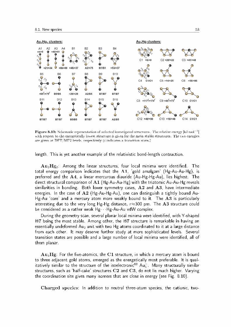
8.1. New species 53

Figure 8.10: Schematic representation of selected investigated structures. The relative energy [kJ mol−1]with respect to the energetically lowest structure is given for the meta-stable structures. The two energiesare given at DFT/MP2 levels, respectively (i indicates a transition state.)

length. This is yet another example of the relativistic bond-length contraction.

Au2Hg2: Among the linear structures, four local minima were identi�ed. Thetotal energy comparison indicates that the A1, 'gold amalgam' (Hg-Au-Au-Hg), ispreferred and the A4, a linear mercurous diauride (Au-Hg-Hg-Au), lies highest. Thedirect structural comparison ofA1 (Hg-Au-Au-Hg) with the triatomic Au-Au-Hg revealssimilarities in bonding. Both lower symmetry cases, A2 and A3, have intermediateenergies. In the case of A2 (Hg-Au-Hg-Au), one can distinguish a tightly bound Au-Hg-Au 'core' and a mercury atom more weakly bound to it. The A3 is particularlyinteresting due to the very long Hg-Hg distance, r≈300 pm. The A3 structure couldbe considered as a rather weak Hg· · ·Hg-Au-Au vdW complex.

During the geometry scan, several planar local minima were identi�ed, with Y-shapedB7 being the most stable. Among other, the B7 structure is remarkable in having anessentially undeformed Au2 unit with two Hg atoms coordinated to it at a large distancefrom each other. It may deserve further study at more sophisticated levels. Severaltransition states are possible and a large number of local minima were identi�ed, all ofthem planar.

Au4Hg: For the �ve-atomics, the C1 structure, in which a mercury atom is boundto three adjacent gold atoms, emerged as the energetically most preferable. It is qual-itatively similar to the structure of the isoelectronic63 Au−5 . Many structurally similarstructures, such as 'half-cake' structures C2 and C3, do not lie much higher. Varyingthe coordination site gives many isomers that are close in energy (see Fig. 8.10).

Charged species: In addition to neutral three-atom species, the cationic, two-

54 8.1. New species

valence-electron [AuHgAu]2+ was also calculated. It is experimentally known in thesolid state.62 The experimental structure is linear with rAu−Hg=278 pm. Our free-ionDFT calculation actually prefers a C2v triangular structure (with rAu−Hg=269 pm) byapproximately +58 and +78 kJ mol−1 at DFT and RIMP2 levels, respectively.

Four-atom charged species were also investigated. The isoelectronic Au42− is pro-

posed as a possible anion in alkali aurides, alkali solutions in liquid ammonia, or similarreducing surroundings. Some occupied MOs of the free ion will then have positive en-ergies, corresponding to continuum states. Concerning Au4

2− at the DFT level, a linearisomer was found to be energetically lowest, with the D3h 'star' (rAu−Au=266.88 pm),and the D4h square (rAu−Au=269.07 pm) higher by +80 and +130 kJ mol−1, respec-tively. At the MP2 level, a linear isomer was still favored, now followed by a C2v rhombusand the D3h star higher. In the case of the isoelectronic Hg2+

4 ion, a linear isomer wasfound to be energetically preferred at both the DFT and MP2 levels. The D3h isomerlies higher by +100 kJ mol−1 and the D4h square by +65 kJ mol−1.

Concerning the structures, both the Hg2+4 and the isoelectronic Au2−

4 chains haveshorter bonds at the ends compared with those at the middle in both our free-moleculecalculations and the solid-state experiment.

Most of the proposed species are new. The likely ways of making these speciesmay involve highly nonequilibrium conditions. Several possible formation paths werediscussed in more detail in Paper VII.

8.2. Molecules as elastic bodies 55

8.2 Molecules as elastic bodies

The �at 2,6-diauro-1,5-naphthyridine polymers, discussed in Section 8.1.3 were bentto closed rings with up to 12 monomers. The structural properties of the rings and thecorresponding �at strips are discussed in Sections 8.1.3 and 8.1.4. In this section wefocus on their vibrational properties, particularly bending energies and lowest in-planedeformation frequencies.

Figure 8.11: Schematic illustration for the bar-type and the ring-type systems. Examples on the con-sidered vibration modes are depicted in F and G.

To understand the connection between the elastic deformation energies, and thevibrational frequencies of the �nite strips and rings, we �rst looked at their classicalcounterparts. Consider �rst a bar segment, as in Fig. 8.11, B. The potential energycontribution due to bending is64

dV =EI

2

(∂2y

∂x2

)2

dx, (8.1)

where E [N m−2] is the Young modulus and I [m4] is the cross-section inertial. Theequation (8.1) corresponds to properties of macroscopic objects and cannot be appliedfor single molecules.

Let us then consider a ring of radius r. For such a system

∂2y

∂x2=

1

r, (8.2)

hence the total bending energy of the ring,

V = πEI

r. (8.3)

56 8.2. Molecules as elastic bodies

Following den Hartog,64 the lowest vibrational angular frequency of a 'free-free bar' (Fig.8.11, C) is

ω =π2

2√

14− 2

π2

√EI

µL4(8.4)

where L is the length, m the mass and µ = m/L the mass per unit length of the bar.Note that ω behaves as L−2. For arbitrary vibrational mode of a ring of radius r in itsown plane, the results of Hoppe65 and Love,66 together with (8.3) give

ω =n(n2 − 1)

r2√

1 + n2

√rV

πµ(8.5)

where n is the number of wavelengths along the ring. This yields a consistency checkbetween V and ω

ω2

V=

1

r3πµ

[n(n2 − 1)]2

1 + n2, (8.6)

which for the lowest mode of the in-plane ring vibration (n=2) gives

ω2

V=

72

5

1

r2m= 14.4r−2m, (8.7)

with m being now the total mass of the ring molecule. By comparing (8.4) and (8.5)and setting n=2, one �nds that the ring of radius r has the same lowest frequency asa bar of length L so that

L2

r2=π3

6

√5

π2 − 8= 8.45, (8.8)

which in turn corresponds to L/r = 2.90, approximately half the ring perimeter.

The low-lying vibrational frequencies should thus behave as L−2 and r−2 for thestrips and rings, respectively. The energy of bending a �at system to a ring of radius rshould go as r−1. We now apply these laws to quantum chemical results.

The analysis of the lowest vibrational modes: Vibrational frequencies werecalculated for the considered strip- and ring-type molecules within harmonic approxima-tion. We focus on the energetically lowest-lying modes, corresponding to the macro-scopic vibrational modes of the sti� slab and the ring (see Fig. 8.11).

Our results calculated for n=2 con�rm the ω(L−2) and ω(r−2)∗ behavior predictedby (8.5). The selected results are presented in Fig. 8.12. For the two higher vibrationalmodes, corresponding to the n=3 and n=4, we also observed similar trends. Thecalculated ratios of slope coe�cients for polyacenes: 1:2.32:4.21, are comparable to thetheoretical values of 1:2.82:5.42 obtained from (8.6) [Paper III, Fig. 9].

For higher values of n, the shortest polyacene 'bars' had to be excluded from consid-eration. With larger n they were found to be too 'short' to reproduce the higher-order

∗Note that L=2πr

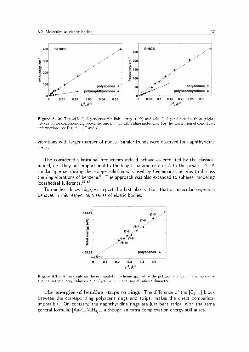
8.2. Molecules as elastic bodies 57

Figure 8.12: The ω(L−2) dependence for �nite strips (left) and ω(r−2) dependence for rings (right)calculated for corresponding polyacene and polynaphthyridine molecules. For the description of considereddeformations see Fig. 8.11, F and G.

vibrations with larger number of nodes. Similar trends were observed for naphthyridineseries.

The considered vibrational frequencies indeed behave as predicted by the classicalmodel, i.e. they are proportional to the length parameter r or L to the power −2. Asimilar approach using the Hoppe solution was used by Ceulemans and Vos to discussthe ring vibrations of benzene.67 The approach was also extended to spheres, modelingicosahedral fullerenes.67,68

To our best knowledge, we report the �rst observation, that a molecular sequencebehaves in this respect as a series of elastic bodies.

Figure 8.13: An example on the extrapolation scheme applied to the polyacene rings. The n=∞ corre-sponds to the energy value on one [C2H4] unit in the ring of in�nite diameter.

The energies of bending strips to rings: The di�erence of the [C2H4] blockbetween the corresponding polyacene rings and strips, makes the direct comparisonimpossible. On contrary, the naphthyridine rings are just bent strips, with the samegeneral formula, [Au2C8N2H4]n, although an extra complexation energy still arises.

58 8.2. Molecules as elastic bodies

Because the closing energy of an in�nite polyacene ring is unknown, it impairs simpleattempt to determine the energy required for bending a strip into a ring, through theirtotal energies. Therefore an alternative reference for the energy of a �at, in�nite polymerwas obtained by letting the ring radius approach in�nity, see Fig. 8.13. We de�ne theextrapolated energy value, ERing(∞), as the energy of one [C2H4] block in the ring ofin�nite diameter. The energy of bending an n-block strip into the ring can then bede�ned as:

∆ERing(n) = ERing(n)− ERing(∞). (8.9)

Here the ERing(n) is the total energy of one [C2H4] unit in the n-unit ring, and the∆ERing(n) is the excess energy per one monomer unit. The total bending energy, V ,of equation (8.3) can then be calculated as

V = n ·∆ERing(n).

Already from Fig. 8.14 one notices that the bending energy indeed behaves as r−1, justas expected from (8.9).

Based on (8.7) we also performed a consistency check between the bending energiesobtained from (8.9) and the lowest frequency modes (n=2). The results are depictedin Fig. 8.14. The �tted slopes of the two lines were calculated to 14.32 and 13.64 forthe polyacene and polynaphthyridine systems, respectively. These can be compared tothe theoretical slope of 72/5=14.4, predicted by equation (8.7).

Figure 8.14: A consistency check between the calculated vibrational frequencies and bending energies.The slopes of the two �tted lines were calculated to 14.32 and 13.64 respectively, as compared to thetheoretical slope of 14.4 calculated from (8.7).

8.3. Basis-set limit of the aurophilic interactions at MP2 level 59

8.3 Basis-set limit of the aurophilic interactions at MP2 level

Many experiments69,70 suggests that, at equilibrium distances of the order of 300 pm,two Au(I) cations in compounds may experience an attraction of the order of 30-40 kJ mol−1. This phenomenon, known as the aurophilic attraction,71 has been exten-sively studied both experimentally and theoretically. For reviews see Ref.1,72

The earliest molecular study (1985) on closed-shell Au(I)-Au(I) systems was of Ho�-mann et al.73 He attributed the aurophilic attraction to the e�ect of hybridizing the6s, 6p, and 5d orbitals of gold. In 1991 Pyykkö and Zhao ascribed this attraction tothe electron correlation e�ect.74 Later in 1997, Pyykkö and Mendizabal provided �rstconclusive evidence for the dispersive nature of the attraction.75,76 They pointed, thatat large distances its strength decreases as R−6. Later studies indicate that close to theequilibrium Au(I)-Au(I) distance, contributions from virtual charge-transfer terms mayalso be important.77

Figure 8.15: The C4v and Td structures of the [P(AuPH3)4]+ ion, C3v structure of the ClAuPH3

monomer and C2 structure of the perpendicular [ClAuPH3]2 dimer.

The applied methodology evolved with time but the studied model remains the same.The commonly accepted system for studies on aurophilicity is the perpendicular dimer[ClAuPH3]2 (Fig. 8.15). Its dimerization energy corresponds to the aurophilic attraction.As suggested by Li and Pyykkö already in 1992,78 due to the nature of this weakintermolecular interaction, the basis-set superposition error (BSSE) corrections must beintroduced. For accurate reproduction of aurophilic attraction certain basis functionsmust also be present in the gold basis set. The di�use s-, p- and d-type functionswere found to have little e�ect. On the contrary, the f-functions were found to beparticularly important. In 1992 Li and Pyykkö introduced a di�use f-function (α = 0.20)that maximizes the Au+ static polarizability, and a tight polarization f-function withα = 1.19. Higher angular-momentum functions have been included for gold by Magnkoet al.79 The basis size of ligands has been studied,80 and was found particularly sensitivefor soft atoms. The basis-set limit of the aurophilic interaction has not been earliercritically investigated. We now investigate it at the MP2 level. We also compare two19-VE pseudopotentials of Andrae et al.81 and the recent one of Figgen et al.82

An additional motivation for such a study is the con�icting results for the pre-ferred conformations of the tetra-aurophosphonium cation (Fig. 8.15), P[AuPH3]

+4 ,

in Ref.80 versus Ref.83 Following the experimental observation of Zeller et al.,84 thatthe [As(AuPPh3)4]

+ ion in solid [As(AuPPh3)4]+[BF4]

− is pyramidal (C4v) and nottetrahedral (Td), Li and Pyykö veri�ed the result using ab-initio calculations. In theircalculations the [N(AuPH3)4]

+, the Td symmetry was preferred, also in agreement with

60 8.3. Basis-set limit of the aurophilic interactions at MP2 level

the experiment. For [P(AuPH3)4]+, a clear preference for C4v was obtained (-90.3 kJ

mol−1). The latter result was supported by Pyykkö and Tamm85 (-76.5 kJ mol−1) butit was recently contested by Fang and Wang83 (+84 kJ mol−1).

[ClAuPH3]2 dimer: The e�ect of choosing the Andrae or Figgen 19-VE pseu-dopotential on the interaction energy ∆E and the Au-Au distance, R, was found to besmall. The di�erence in ∆E, due to the choice of PP, reaches up to 0.15 kJ mol−1. Thedi�erence in Re increases slightly with basis size but remains less than 0.5 pm even forthe largest considered basis. Di�erent pseudopotentials yield a negligible error [PaperIV, Table 2].

For the study on the basis-set limit, several Karlsruhe split-valence basis sets (def-X and def2-X, X=SVP-QZVPP) and their augmented versions were applied. Theaugmentation refers to adding two f-type functions (α=0.20, 1.19) of Pyykkö et al.80

All considered basis sets were augmented using two schemes: the f-functions were addedas uncontracted (-A), and contracted (-B). Application of bases with two uncontractedf-functions for Au, lowers the value of ∆ECP and leads to faster and more systematicconvergence.

The previously reported ∆ECP for dimer, calculated by Li and Pyykkö80 was obtainedwith approximately TZVP-quality basis set with two uncontracted f-functions and withAndrae ECP applied. The resulting value of -24.70 kJ mol−1 corresponds to the presentlyreported value of -22.94 kJ mol−1 obtained with a slightly larger Karlsruhe def2-TZVPbasis set augmented with the two f-functions for consistency.

The basis-set size dependence of the counterpoise correction to the calculated ∆Ewas investigated. The di�erences between counterpoise-corrected ∆ECP and uncor-rected ∆E values are depicted in Fig. 8.16. We emphasize that if the counterpoisecorrection is not applied, the BSSE leads to a large discrepancy, especially for smallerbasis sets. Interestingly, even though the energy gap closes with the larger basis sets, itremains as wide as +10 kJ mol−1 at the QZVPP level, because higher angular momen-tum functions are required to close that gap. Even at the QZVPP level the basis setlimit is not reached. The best obtained result, corresponding to def2-QZVPP+2f basisset, is -33.41 kJ mol−1. This value is expected to be close to the basis set limit for theMP2 method.

P[AuPH3]+4 cation: To �nd the source of discrepancy in the preferred structure,

we �rst investigated the di�erence in ∆E=E(C4v)-E(Td) due to the two di�erent 19-VE pseudopotentials of Andrae, used by Pyykkö et al., and the one of Figgen, appliedby Fang and Wang. We found the di�erence to be negligible. Only at the QZVPP leveldoes it exceed 1 kJ mol−1. The choice of the PP also does not a�ect the symmetryof the cation. The more general aspects of PP in�uence on the Au(I)-Au(I) interactionhave already been investigated by Pyykkö et al.75,76,86

We then turned our attention to the basis sets. We found that, in the case of the olderKarlsruhe basis sets (def-X), especially the smaller sets are too poor in higher angularmomentum basis-functions to properly describe the closed-shell aurophilic interactions.Augmentation with two contracted f-functions (-B) yields mainly negative ∆E values,with C4v symmetry preferred. By adding the two uncontracted f-functions (-A), the


Figure 8.16: Comparison of the calculated, noncounterpoise-corrected ∆E and corrected ∆ECP valuesfor [ClAuPH3]2 dimer, obtained using original def2-X Karlsruhe and augmented def2-X-A bases (-Astands for two uncontracted f-functions, α=0.20, 1.19).

convergence level is achieved already at the TZVP level (see Fig. 8.17).The latest generation of basis sets (def2-X) contains at least one f-function (α=0.72)

on gold, even for the smallest def2-SVP basis set. Although the application of newerbasis sets lowers the calculated ∆E, as compared to the corresponding older def-Xsets, the f-subspace is still too small, and additional enrichment with more f-functions ishelpful. As expected, it also is better to add two uncontracted f-functions rather thankeep them contracted.

Figure 8.17: The comparison of calculated ∆E=E(C4v)-E(Td) energies for [P(AuPH3)4]+ ion, obtained

using the original split-valence (def-X and def2-X) and correlation-consistent (cc-pVY Z) basis sets, withthe ∆E values obtained in the same sets augmented with two uncontracted (-A) and two contracted (-B)f-type functions (α = 0.20, 1.19).

In the case of both def-X and def2-X basis sets, adding the two f-functions to thesmallest SVP sets, will lead to a large overestimation of ∆E, even by a factor of 4(see Fig. 8.17, left and center). The larger sets contain already enough higher angularmomentum functions (f and higher). The addition of two extra f-functions does notmake a substantial di�erence. It also explains why the ∆E values obtained previouslyby Pyykkö and co-workers were more negative. Most likely, the employed basis sets werestill too small to give results close to the convergence limit. Nevertheless, the qualitativeresults of the previous studies are recon�rmed.

Our currently best estimate for ∆E, calculated with largest Karlsruhe split-valence

62 8.3. Basis-set limit of the aurophilic interactions at MP2 level

basis sets, is -15.0 kJ mol−1. It is in good agreement with the calculations performedwith the correlation-consistent basis sets (Fig. 8.17, right). For the cc basis sets, we alsoperformed the two-point basis-set extrapolation87 based on the total energies calculatedfor the Td and C4v isomers. The ∆E calculated at the basis-set limit is estimated to-14.5 kJ mol−1. Finally, the comparison with the value of -13.74 kJ mol−1 calculatedwith the full cc-pV5Z basis, yields a satisfactory agreement. Both the results obtainedwith the split-valence and the cc type basis sets, converge to the similar result.

In none of the studied cases were we able to reproduce the positive value of ∆E=+84kJ mol−1 reported by Fang and Wang.83 The C4v symmetry is still favored at the MP2level.

SCS-MP2: [ClAuPH3]2 dimer

It is known that MP2 method tends to overestimate aurophilic attraction. Forcertain small cases, such as the 'classical' dimer model (see Fig. 8.15), it is still possibleto calculate the interaction energy, ∆ECP (R), even at the Coupled-Cluster level.

Fig. 8.18 illustrates a comparison of high-accuracy Coupled-Cluster results with thosecalculated using standard MP2 and the recently introduced SCS-MP2 method. Weemphasize an excellent agreement between the CCSD(T) and much less expensive SCS-MP2 results.

Figure 8.18: A comparison of CC methods with standard MP2 and empirically corrected SOS-MP2 andSCS-MP2 methods.

SCS-MP2: [P(AuPH3)4]+ cation

Following the observation that the Spin-Component-Scaled MP2 results for the[ClAuPH3]2 dimer are in a signi�cantly better agreement with CCSD(T) than with theMP2 ones, we have recalculated the ∆E=E(C4v)-E(Td) using the SCS-MP2 scheme.


Using a su�ciently large, split-valence quadruple-zeta quality basis sets, we re-produced our earlier result for MP2 (∆E=-16.2 kJ mol−1). The SCS-MP2 yields∆E=+19.8 kJ mol−1 and the SOS-MP2 yields ∆E=+37.8 kJ mol−1. Both meth-ods favor Td symmetry.

64 8.4. High-accuracy calculations of MCN, M=Cu-Au

8.4 High-accuracy calculations of MCN, M=Cu-Au

The AuCN molecule is important because it is related to the [Au(CN)2]− ion, which

is used in most of the gold production in the world. It is also interesting from the pointof view of this thesis, as AuCN and similar cyanides can be considered as monomers inthe formation of 2D crystals discussed in Paper I. Experimental studies on solid MCN(M=Cu, Ag, Au) exist.88,89,90,91 Molecular calculations were reported by Boldyrev etal.,92 Dietz et al.,93 Grotjahn et al.,94 Lee et al.,95 Veldkamp et al.96 and Schwerdtfegeret al.97

Experimental structural data for gas-phase AuCN have been reported recently.98

Understanding the qualitative aspects of molecular bonding was thus of interest. Ourcalculated M -C bond lengths are only slightly larger than the sum of the triple-bondcovalent radii99 indicating complex, multiple-bond character of that bond. For mostaccurate results, we applied Coupled-Cluster theory. We compare those with resultsfrom commonly used second-order Møller-Plesset perturbation approach (MP2). Simi-lar calculations, have appeared but with relatively small basis sets. We now performedboth MP2 and CCSD(T) calculations using the newest pseudopotentials82 for the metaland large basis sets.100

An example on AuCN

Level of electron correlation: Table 8.5 summarizes results obtained by theMP2 and CCSD(T) methods. We found that the MP2 method fails to describe theAuCN molecule accurately. The Au-C distance obtained using a cc-pVQZ basis set de-viates from the experimental value by -2.5 %, while the CCSD(T) one is in much betteragreement with experiment. For the C-N distance, MP2 also is worse than CCSD(T).Similar relative trends were found for the CuCN and AgCN molecules [Paper V].

E�ect of freezing the core: The gold cyanide molecule with 19-VE Au and all-electron C and N has 16 occupied molecular orbitals. In order to save computationaltime, one would typically freeze some, or all, of the six occupied MOs below the tentop ones in Fig. 8.19. From below, they are MO1 1sC, MO2 1sN, MO3 5sAu, and the

Method Basis/frozen MOs Au-C C-N ω1 ω2 ω3

CCSD(T) cc-pVQZ/none 191.12 116.23 2215 289 482cc-pVQZ/MO1−2 191.26 116.50 2203 284 480cc-pVQZ/MO1−3 191.14 116.50 2203 285 481cc-pVQZ/MO1−6 192.10 116.50 2202 278 471

Expt. (g) Ref.98 191.22519(84) 115.86545(97) - 320 480

Table 8.4: Selected calculated bond lengths [pm] and harmonic vibrational modes [cm−1] for MCN(M=Cu, Ag, Au)

8.4. High-accuracy calculations of MCN, M=Cu-Au 65

Method/Case Au-C C-N ω1 ω2 ω3

AuCNCCSD(T) cc-pVDZ 191.85 118.31 2183 282 486

cc-pVTZ 190.97 116.50 2214 292 481cc-pVQZ 191.12 116.23 2215 289 482

MP2 cc-pVDZ 187.63 118.95 2096 298 521cc-pVTZ 186.41 117.16 2128 312 520cc-pVQZ 186.51 116.92 2127 309 520

Expt. (g) Ref.98 191.22519(84) 115.86545(97) - 320 480Expt. (s) Ref.88 197.175 115.474 - - -

AgCNCCSD(T) cc-pVDZ 201.52 118.40 2172 240 406

cc-pVTZ 202.16 116.59 2201 234 397cc-pVQZ 202.04 116.33 2203 221 402

Expt. (g) Ref.98 203.1197(23) 116.0260(26) - 240 400Expt. (s) Ref.89 206.00 116.00 - - -

CuCNCCSD(T) cc-pVDZ 180.49 118.49 2172 305 492

cc-pVTZ 181.96 116.66 2203 262 479cc-pVQZ 181.85 116.39 2204 255 483

Expt. (g) Ref.98 182.962(4) 116.213(3) - 270 478Expt. (s) Ref.90 184.60 117.00 2170 - -

Table 8.5: Selected calculated bond lengths [pm] and harmonic vibrational modes [cm−1] for MCN(M=Cu, Ag, Au)

three MO4−6 5pAu. The e�ect of freezing selected electrons in AuCN is summarized inTable 8.4. Unfreezing the 5pAu shortens the Au-C distance by 1 pm. Deeper excitationshave a small e�ect. The C-N distance is not a�ected by 'opening' the Au orbitals. It isshortened by as much as 0.3 pm if the MO1−2 are correlated as well. The e�ect on theAu-C-N bend, ω2, parallels that on the Au-C distance. The stretching ω3 is in�uencedby opening the 5pAu. The C-N stretch, ω1, is increased by 13 cm−1 if the 1s shells,MO1−2, are correlated.

Basis-set-size e�ect: The errors of the calculated Au-C and C-N distances clearlydiminish from DZ to TZ basis. The errors diminish even further from TZ to QZ andthe smallness suggests adequate convergence (Table 8.5). Change from the smallest,cc-pVDZ, to the largest cc-pVQZ basis lowers the relative errors roughly by a factor of7 for both Au-C and C-N distances. The CCSD(T) harmonic vibrational frequencies,calculated with the three basis sets of di�erent quality, yield a similar picture. For theC-N stretch, not even an experimental estimate is available. Because the rotationalspectroscopy gives the vibrational wavenumbers only indirectly, the experimental values


Figure 8.19: The ten highest occupied Hartree-Fock MO, of AuCN. The Kohn-Sham MOs look verysimilar. The bottom row depicts orbitals important for bonding.

of ω2 and ω3 are only rough estimates.

Spin-orbit e�ects: The calculations with spin-orbit e�ects, obtained at the DFTlevel, yield bond lengths in good agreement with the known experimental values andalso with the present CCSD(T) calculations. The spin-orbit e�ects on bond lengths aresmall and rise to -0.38 pm for the Au-C distance in AuCN. The magnitude grows withthe nuclear charge of the metal atom.

Anharmonicity: The experimental estimates reported by Okabayashi et al. forMCN (M=Cu, Ag, Au) are based on the harmonic approximation, hence the goodagreement with calculated CCSD(T) harmonic values. We estimated the error intro-duced by the harmonic approximation at the MP2 level using cc-pVTZ basis sets (PaperV, Table VII). In each case, the anharmonicities lower the calculated frequency. Theanharmonic correction, ∆, decreases strongly with Z. In case of the C-N stretch, ∆ isapproximately -33 cm−1 and remains constant for all analyzed cyanides.

Qualitative bonding analysis: The experimental M -C (M=Cu, Ag, Au) areonly a few picometers longer than those predicted by the triple-bond covalent radii (by3, 6, and 8 pm). Among the occupied MOs depicted in Fig. 8.19 we indeed �nd thebonding orbitals HOMO-6,7. The higher-lying HOMO-1 and HOMO-2 is basically thecyanide π. Interestingly, the Au-C bonding occurs both in the HOMO, and there pri-marily to the gold 'doughnut' hybrid, and in the lower-lying HOMO-8.

Our best-estimated results for studied cyanides are presented in Table 8.6. TheM -C distances agree with experiments within about 0.6 pm or even better. The M -Cbond-length trend for the four metals is Cu < Rg < Au < Ag. We emphasize the sig-ni�cance of the BSSE. The remaining di�erence may come from the rs, re, and the rmde�nitions, the pseudopotential approximation, coupled-clusters perturbative triplets, orother sources. Our calculated harmonic frequencies are expected to be more accuratethan available gas-phase experimental estimates.94,98

8.4. High-accuracy calculations of MCN, M=Cu-Au 67

Metal Cu Ag Au

M -C 181.85 202.04 191.12BSSE +0.52 +0.47 +0.31SO -0.01 -0.09 -0.38Best est. 182.36 202.42 191.05Expt. 182.962(4)c 203.1197(23)d 191.22519(84)d

C-N 116.39 116.33 116.23SO +0.01 +0.07 0.00Best est. 116.40 116.40 116.23Expt. 116.213(3)c 116.0260(26)d 115.86545(97)d

ω1

Best CCSD(T)a 2204 2203 2215Best est. 2171 2171 2181Expt. est. - - -Expt. est. + ∆ - - -

ω3

Best CCSD(T)a 255 221 289Best est. 232 209 285Expt. est. 270c 240d 320d

Expt. est. + ∆ 247 228 316

ω3

Best CCSD(T)a 483 402 482Best est. 439 378 472Expt. est. 478c 400d 480d

Expt. est. + ∆ 434 376 470

aCCSD(T)/cc-pVQZ, bPBE-ZORA/QZ4P, cRef.,94 dRef.98

Table 8.6: The best estimated values for bond lengths and vibrational harmonc modes forMCN (M=Cu,Ag, Au).

References

[1] Pyykkö, P. Angew. Chem. Int. Ed. 2004, 43, 4412.

[2] Häkkinen, H. Chem. Soc. Rev. 2008, 37, 1847.

[3] Møller, C.; Plesset, M. S. Phys. Rev. 1934, 46, 618.

[4] Pople, J. A.; Binkley, J. S.; Seeger, R. Int. J. Quant. Chem. 1976, 10, 1.

[5] Schwabe, T.; Grimme, S. Acc. Chem. Research 2008, 41, 569.

[6] Grimme, S. J. Chem. Phys. 2003, 118, 9095.

[7] Langho�, S. R.; Davison, E. R. Int. J. Qunat. Chem. 1974, 8, 61.

[8] Pople, J. A.; Head-Gordon, M.; Raghavachari, K. J. J. Chem. Phys. 1987, 87,5968.

[9] Mazziotti, D. A. Phys. Rev. Letters 2004, 93, 213001.

[10] Hohenberg, P.; Kohn, W. Phys. Rev. 1964, 136, B864.

[11] Kohn, W.; Sham, L. J. Phys. Rev. 1965, 140, A1133.

[12] Becke, A. D. Phys. Rev. A 1986, 33, 2786.

[13] Perdew, J. P.; Burke, K.; Ernzerhof, M. Phys. Rev. Letters 1996, 77, 3865.

[14] Becke, A. D. Phys. Rev. A 1988, 38, 3098.

[15] Lee, C.; Yang, W.; Parr, R. G. Phys. Rev. B 1988, 37, 785.

[16] Vosko, S. H.; Wilk, L.; Nusair, M. Can. J. Phys. 1980, 58, 1200.

[17] Tao, J.; Perdew, J. P.; Staroverov, V. N.; Scuseria, G. E. Phys. Rev. Letters2003, 91, 146401.

[18] Perdew, J. P.; Kurth, S.; Zupan, A.; Blaha, P. Phys. Rev. Letters 1999, 82,2544.

[19] Alloutia, F.; Mancerona, L.; Alikhani, M. E. J. Mol. Struc. 2009, 903, 4.

[20] Görling, A.; Levy, M. Phys. Rev. B 1993, 47, 13105.

[21] Görling, A.; Levy, M. Phys. Rev. A 1994, 50, 196.

[22] Schwabe, T.; Grimme, S. Phys. Chem. Chem. Phys. 2007, 9, 3397.

69

70 References

[23] Koch, W.; Holthausen, M. C. A Chemist's Guide to Density Functional Theory;Wiley-VCH: Weinheim,.

[24] Ibach, H. Solid-State Physics, An Introduction to Principles of Materials Science;Springer-Verlag: 1996.

[25] Chadi, D. L.; Cohen, M. L. Phys. Rev. B 1973, 8, 5747.

[26] Monkhorst, H. J.; Pack, J. D. Phys. Rev. B 1976, 13, 5188.

[27] Born, M.; Oppenheimer, R. Ann. Phys. (Leipzig) 1927, 84, 457.

[28] Stanke, M.; Kedziera, D.; Bubin, S.; Adamowicz, L. J. Chem. Phys. 2007, 127,134107.

[29] Stanke, M.; Komasa, J.; Kedziera, D.; Bubin, S.; Adamowicz, L. Phys. Rev. A2008, 77, 062509.

[30] Valeev, E. F.; Sherrill, C. D. J. Chem. Phys. 2003, 118, 3921.

[31] Francis, G. P.; Payne, M. C. J. Phys. Cond. Matt. 1990, 2, 4395.

[32] Martin, J. M. L.; Taylor, P. R. Chemical Physics Letters 1994, 225, 473 - 479.

[33] Martin, J. M. L.; Taylor, P. R. Chemical Physics Letters 1996, 248, 336 - 344.

[34] Martin, J. M. L. Chemical Physics Letters 1995, 242, 343 - 350.

[35] Levine, I. N. Quantum Chemistry; Prentice-Hall: 1991.

[36] Helgaker, T.; Klopper, W.; Tew, D. P. Mol. Phys. 2008, 106, 2107.

[37] Dunlap, B. I.; Connolly, J. W. D.; Sabin, J. R. J. Chem. Phys. 1979, 71, 3396.

[38] Bethe, H. A.; Salpeter, E. E. Quantum Mechanics of One- and Two-ElectronAtoms; Plenum Press: 1977.

[39] Douglas, M.; Kroll, N. M. Ann. Phys. 1974, 82, 89.

[40] Jansen, G.; Hess, B. A. Phys. Rev. A 1989, 39, 6016.

[41] Barysz, M. J. Chem. Phys. 2001, 114, 9315.

[42] Reiher, M.; Wolf, A. Relativistic Quantum Chemistry, The Fundamental Theoryof Molecular Science; Wiley-VCH: Weinheim, 2009.

[43] Dyall, K. J. Chem. Phys. 1997, 106, 9618.

[44] Filatov, M.; Cramer, D. J. Chem. Phys. 2003, 118, 7641.

[45] Barysz, M.; Sadlej, A. J. J. Chem. Phys. 2003, 116, 2696.

[46] Kutzelnigg, W.; Liu, W. J. Chem. Phys. 2005, 123, 241102.

[47] Zhdanov, G. S.; Shugam, E. A. Zh. Fiz. Khim. 1945, 19, 519.

[48] Hakala, M. O.; Pyykkö, P. Chem. Comm. 2006, 2006, 2890.

References 71

[49] Wang, H. M. J.; Lin, I. J. B. Organometallics 1998, 17, 972.

[50] Vaughan, L. G. J. Am. Chem. Soc. 1970, 92, 730.

[51] Vaughan, L. G. J. Organomet. Chem. 1980, 190, C56.

[52] Naumkin, F. Phys. Chem. Chem. Phys. 2006, 8, 2539.

[53] Gibson, J. K. J. Vac. Sci. Technol. 1998, 16, 653.

[54] Pyykkö, P.; Patzschke, M.; Suurpere, J. Chem. Phys. Letters 2003, 381, 45.

[55] Sneed, M. C.; Maynard, J. L.; Brasted, R. C. Comprehensive Inorganic Chemistry,Vol. 2; D. van Nostrand Co., Inc.: , 1954.

[56] Rykova, E. A.; Zaitsevskii, A.; Mosyagin, N. S.; Isaev, T. A.; Titov, A. V. J.Chem. Phys. 2006, 125, 241102.

[57] Wesendrup, R.; Laerdahl, J. K.; Schwerdtfeger, P. J. Chem. Phys. 1999, 110,9457.

[58] Gillespie, R. J.; Granger, P.; Morgan, K. R.; Schrobilgen, G. J. Inorg. Chem.1984, 23, 887.

[59] Kertesz, M.; Guloy, A. M. Inorg. Chem. 1987, 26, 2852.

[60] Cutforth, B. D.; Gillespie, R. J.; Ireland, P.; Sawyer, J. F.; Ummat, P. K. Inorg.Chem. 1983, 22, 1344.

[61] Brown, I. D.; Gillespie, R. J.; Morgan, K. R.; Sawyer, J. F.; Schmidt, K. J.;Tun, Z.; Ummat, P. K. Inorg. Chem. 1987, 26, 689.

[62] Catalano, V. J.; Malwitz, M. A.; Noll, B. C. Chem. Commun. 2001, 2001, 581.

[63] Furche, F.; Ahlrichs, R.; Weis, P.; Jacob, C.; Gilb, S.; Bierweiler, T.; Kappes, M.M. J. Chem. Phys. 2002, 117, 6982.

[64] Den Hartog, J. P. Mechanical Vibrations; McGraw-Hill: New York, London, 1947.

[65] Hoppe, R. J. Reine Angew. Math. 1871, 73, 158.

[66] Love, A. E. H. Proc. London Math. Soc. 1893, 24, 118.

[67] Ceulemans, A.; Vos, I. Mol. Phys. 1991, 72, 1051.

[68] Ceulemans, A.; Fowler, P. W.; Vos, I. J. Chem. Phys. 1994, 100, 5491.

[69] Schmidbaur, H.; Graf, W.; Müller, G. Angew. Chem. 1988, 100, 439.

[70] Melnik, M.; Parish, R. V. Coord. Chem. Rev. 1986, 70, 157.

[71] Scherbaum, F.; Grohmann, A.; Huber, B.; Krüger, C.; Schmidbaur, H. Angew.Chem. 1988, 100, 1602.

[72] Schmidbaur, H. Gold Bull. 1990, 23, 11.

[73] Jiang, Y.; Alvarez, S.; Ho�mann, R. Inorg. Chem. 1985, 24, 749.

72 References

[74] Pyykkö, P.; Zhao, Y.-F. Angew. Chem. 1991, 103, 622 Angew. Chem. Int. Ed.Engl., 30, 604, (1991).

[75] Pyykkö, P.; Runeberg, N.; Mendizabal, F. Chem. Eur. J. 1997, 3, 1451.

[76] Pyykkö, P.; Mendizabal, F. Chem. Eur. J. 1997, 3, 1458.

[77] Runeberg, N.; Schütz, M.; Werner, H.-J. J. Chem. Phys. 1999, 110, 7210.

[78] Li, J.; Pyykkö, P. Chem. Phys. Letters 1992, 197, 586.

[79] Magnko, L.; Schweizer, M.; Rauhut, G.; Schütz, M.; Stoll, H.; Werner, H.-J.Phys. Chem. Chem. Phys. 2002, 4, 1006.

[80] Li, J.; Pyykkö, P. Inorg. Chem. 1993, 32, 2630.

[81] Andrae, D.; Häuÿermann, U.; Dolg, M.; Stoll, H.; Preuÿ, H. Theor. Chim. Acta1990, 77, 129.

[82] Figgen, D.; Rauhut, G.; Dolg, M.; Stoll, H. Chem. Phys. 2005, 311, 227.

[83] Fang, H.; Wang, S.-G. J. Phys. Chem. A. 2006, 111, 1562.

[84] Zeller, E.; Beruda, H.; Kolb, H.; Bissinger, A.; Riede, P.; Schmidbaur, J. Nature1991, 352, 141.

[85] Pyykkö, P.; Tamm, T. Organometallics 1998, 17, 4842.

[86] Pyykkö, P.; Mendizabal, F. Inorg. Chem. 1998, 37, 3018.

[87] Helgaker, T.; Jørgensen, P.; Olsen, J. Molecular Electronic-Structure Theory;Wiley: Chichester, 2000.

[88] Hibble, S. J.; Hannon, A. C.; ; Cheyne, S. M. Inorg. Chem. 2003, 42, 4724.

[89] Hibble, S. J.; Cheyne, S. M.; Hannon, A. C.; Evers�eld, S. G. Inorg. Chem.2002, 41, 1042.

[90] Hibble, S. J.; Cheyne, S. M.; Hannon, A. C.; Evers�eld, S. G. Inorg. Chem.2002, 41, 4990.

[91] Bowmaker, G. A.; Kennedy, B. J.; Reid, J. C. Inorg. Chem. 1998, 37, 3968.

[92] Boldyrev, A. I.; Li, X.; Wang, L.-S. J. Chem. Phys. 2000, 112, 3627.

[93] Dietz, O.; Rayón, V. M.; Frenking, G. Inorg. Chem. 2003, 42, 4977.

[94] Grotjahn, D. B.; Brewster, M. A.; Ziurys, L. M. J. Am. Chem. Soc. 2001, 124,5895.

[95] Lee, D.; Lim, I. S.; Lee, Y. S.; Hagebaum-Reignier, D.; Jeung, G.-H. J. Chem.Phys. 2007, 126, 244313.

[96] Veldkamp, A.; Frenking, G. Organometallics 1993, 12, 4613.

[97] Schwerdtfeger, P.; Boyd, P. D. W.; Burrell, A. K.; Taylor, M. J. Inorg. Chem.1990, 29, 3593.

References 73

[98] Okabayashi, E. Y.; Okabayashi, T.; Koto, F.; Tanimoto, M. Presented at the61st Ohio State University International Symposium on Molecular Spectroscopy,Columbus, OH, 2006, Paper No. RE09. .

[99] Pyykkö, P.; Riedel, S.; Patzschke, M. Chemistry 2005, 11, 3511.

[100] Peterson, K. A.; Puzzarini, C. Theor. Chem. Acc. 2005, 114, 283.

computational studies on new chemical species in the gas

Documents