computational methods and theoretical results for the ka

TMO Progress Report 42-140 February 15, 2000

Computational Methods and Theoretical Resultsfor the Ka-Band Array Feed Compensation

System–Deformable Flat PlateExperiment at DSS 14

W. A. Imbriale1 and D. J. Hoppe1

This article documents the computational methods and theoretical results for thedeformable flat plate (DFP), array feed compensation system (AFCS), monopulsetracking system, and combined AFCS–DFP used for compensating the gravity-induced distortions on the DSN’s 70-m antenna. These systems were utilized in anexperiment designed to verify gravity compensation and tracking performance ofthe 70-m antenna at 31.8–32.2 GHz (Ka-band). This experiment took place fromNovember 1998 through February 1999 and consisted of both quasar and spacecraftobservations. The theoretical results are compared with the experimental data.The analytical tools are also used to document and understand the characteristicsof each system.

I. Introduction

During the period from November 1998 through February 1999, a series of measurements was carriedout on the 70-m antenna at DSS 14 to determine the performance characteristics of two systems designedto compensate for the effects of elevation-dependent gravity distortion of the main reflector on antennagain. The array feed compensation system (AFCS) and the deformable flat plate (DFP) system bothwere mounted on the same feed cone, and each was used independently as well as jointly to measureand improve the antenna aperture efficiency as a function of elevation angle. The experimental data arepresented in [1] and [2].

This article contains a description of the computational method and theoretical results for the DFP,the AFCS, the monopulse tracking system, and the combined AFCS–DFP system.

The basic analysis tool is a physical optics reflector-analysis code that was ported to a parallel computerfor faster execution times. There are several steps involved in computing the RF performance of thevarious systems:

1 Communications Ground Systems Section.

1

(1) A model of the RF distortions of the main reflector is required. This model is based uponmeasured holography maps of the 70-m antenna obtained at three elevation angles. Theholography maps then are processed (using an appropriate gravity mechanical model ofthe dish) to provide surface distortion maps at all elevation angles. This technique isfurther described in [3].

(2) From the surface distortion maps, ray optics is used to determine the theoretical shapeof the DFP that will exactly phase compensate the distortions.

(3) From the theoretical shape and a NASTRAN mechanical model of the plate, the actuatorpositions that generate a surface that provides the best rms fit to the theoretical modelare selected. Using the actuator positions and the NASTRAN model provides an accuratedescription of the actual mirror shape.

(4) Starting from the mechanical drawings of the feed, a computed RF feed pattern is gen-erated. This pattern is expanded into a set of spherical wave modes so that a completenear-field analysis of the reflector system can be obtained.

(5) For the array feed, the excitation coefficients that provide the maximum gain are com-puted using a phase conjugate technique.

The basic experimental geometry consisted of a dual-shaped 70-m antenna system, a refocusing ellipse,a DFP, and an array feed system. To provide physical insight into the systems performance, focal planefield plots are presented at several elevations. Curves of predicted performance are shown for the DFPsystem, monopulse tracking system, AFCS, and combined DFP–AFCS system. The calculated resultsshow that the combined DFP–AFCS system is capable of recovering the majority of the gain lost due togravity distortion.

II. Geometry

The experiment geometry is shown in Fig. 1. The main elements are the 70-m main reflector andsubreflector, a refocusing ellipse, the DFP, and the receive feed system. The focal point of the dual-reflector 70-m system is labeled F1, and the focal point where the feed is placed is labeled F2. The antennaCassegrain focus was 0.6 in. (1.5 cm) above F1, which was corrected for alignment of the subreflector inthe z-axis. Looking at the system in the transmit mode, the output of the feed system is refocused at F1,the input to the dual-reflector system. The parameters of the ellipse are chosen to map the fields (withno magnification) from F2 to F1. Hence, the performance of the 70-m system would be the same if thesame feed were placed at either F1 or F2.

A. Ray-Based Computation of the Deformable-Mirror Surface

In this section, a description of the steps involved in the computation of the deformable-mirror surfaceis provided. The process begins with a processed holography map describing the main-reflector distortionsto be corrected for at the elevation angle of interest. The final output of the design process is the surfaceof the deformable mirror required to correct for those distortions. Three main computer programs areinvolved. The process is summarized in the flow chart presented in Fig. 2 and in the following paragraphs.

1. Step 1: Zernike Coefficient Computation. The first step in the design process is to process theholography maps described earlier in the article for use in the computation. Due to the large size of thereflectors relative to the wavelength at 32 GHz, it was decided to ignore diffraction in the computation ofthe deformable-mirror surface. A ray-based analysis code, Modeling and Analysis for Controlled OpticalSystems (MACOS) [4], is used to trace the deformations on the main reflector to the deformable mirror.With MACOS, arbitrary surfaces such as the distorted-shaped reflectors of DSS 14 are described using aZernike expansion. The nominal shaped subreflector and main-reflector surfaces and the main-reflectordistortion require Zernike expansions.

2

CASSEGRAINFOCUS 0.6 in. (1.5 cm)

F1

16.2 in.(41.1 cm)

DFP

ELLIPSOID

C

B

A22-dB HORN

10.8 in.(27.4 cm)

27 in. (68.6 cm)

1 in. (2.5 cm)

F2

61.5 in. (156.2 cm)

34.5 in.(87.6 cm)

53o53o

Fig. 1. The RF optics design inside the holography cone, showingthe geometry that enables both separate AFCS and DFP measure-ments at F1 and F2, respectively, and joint AFCS-DFP measure-ments at F2.

As illustrated in Fig. 2, the program DFM.EXE computes the Zernike coefficients for a given main-reflector distortion. The distortion is described via a processed holography map, typically on a 127-by-127 point square grid encompassing the main reflector. Additional information such as the grid spacing,frequency, reflector diameter, and best-fit parabola are included in an additional data file. This data filealso includes details regarding any masks that must be applied to the holography map. Shadowed areasof the main reflector are masked. These included strut shadows and the center of the reflector where thetricone structure is located. These areas receive essentially zero amplitude illumination and, hence, thephase data in these areas cannot be used to deduce the surface distortion. The masks are employed asfollows. The main-reflector distortions in the masked areas are initially set to zero. An initial Zernikeseries is computed. The Zernike series then is used to fill in an approximate distortion in the maskedareas, and a new Zernike series is computed. The process is repeated until convergence of the Zernikecoefficients is achieved. Less than 10 iterations of this process results in a smooth extrapolation of thesurface distortion into the masked areas.

The deformable-mirror surfaces computed for this work were based on including 91 terms in theZernike expansion of the main-reflector distortions. Although including more terms would better modelhigher-order surface distortions in the main reflector, including them was found to have essentially noimpact on the final actuator positions computed for the deformable mirror. This is expected since theactuator density on the mirror determines the scale of distortion that may be corrected. In this case,the resolution of the actuators is already greatly exceeded by the 91-term Zernike expansion of the main-reflector distortion.

3

HOLOGRAPHY MAP FORELEVATION ANGLE OF

INTEREST

DFM.EXE

ZERNIKE SERIES LIMITS,FREQUENCY, OTHER

DATAZERNIKE COEFFICIENTS

REPRESENTING THEDISTORTION

MACOS.EXENOMINAL REFLECTORSHAPES, REFLECTOR

POSITIONS, ETC.

INFORMATION ON RAYSPROPAGATING TOWARDDEFORMABLE MIRROR

PL.EXEPLATE LOCATION, FOCALPOINT LOCATION, PATH

LENGTH, ETC.

POINT-WISE DESCRIPTION OFTHE DEFORMABLE MIRROR’S

SHAPE

Fig. 2. Flow chart describing the computation of thedeformable mirror.

2. Step 2: Ray Trace of the Distorted-Reflector System. As mentioned above, due to the largesize of the reflectors on DSS 14 in terms of wavelengths at 32 GHz, a ray-based approach to determiningthe deformable-mirror surface is deemed satisfactory. The validity of this assumption is tested in asubsequent section of this article, where physical optics (PO), which takes into account diffraction effects,is used to evaluate the performance of the system. A modified version of MACOS, a JPL-produced code,was used to trace the rays through the distorted-reflector system. The code was modified to increase themaximum number of terms in the Zernike expansion of the surfaces. Due to details regarding the mannerin which arbitrary surfaces are handled in MACOS, this modification turned out to be non-trivial.

As illustrated in Fig. 2, the Zernike coefficients for the distortion are combined with the file describingthe nominal-reflector system geometry and fed into MACOS. The shaped subreflector and main reflectorare described by 21-term, rotationally symmetric, Zernike expansions. The additional Zernike termsdescribing the deformation then are added to the nominal main-reflector surface description. The ellipsoid,which refocuses the incoming radiation through the deformable mirror to the remote feed location, alsois included in the model. All hardware locations and rotations are included in the model.

The analysis begins by launching a bundle of approximately 4000 rays into the main reflector. Masksare applied, limiting the maximum diameter of the main reflector and subreflector. An additional mask isapplied to eliminate the tricone area of the main-reflector surface. The rays are traced to the subreflectorand finally to the ellipsoid, where they are reflected toward the deformable mirror. Figure 3 shows a low-resolution two-dimensional plot of the reflector geometry and a subset of rays. The output capabilities of

4

(b)

-100 0 100

Z-AXIS

200 300 400 500

-100

0

100

X-A

XIS

Fig. 3. Ray traces: (a) main reflector to focal plane and (b) subreflector to focal plane.

-500 0 500

Z-AXIS

(a)

-1000

-500

0

500

1000

X-A

XIS

5

MACOS then are employed to generate an output file containing the ray positions, directions, and ray-pathlengths immediately after reflection from the ellipsoid. For a typical run, this file contains informationon approximately 3200 rays that survive the masking operations. The ray information contained in thisfile then is employed in the last step of the process, as described below.

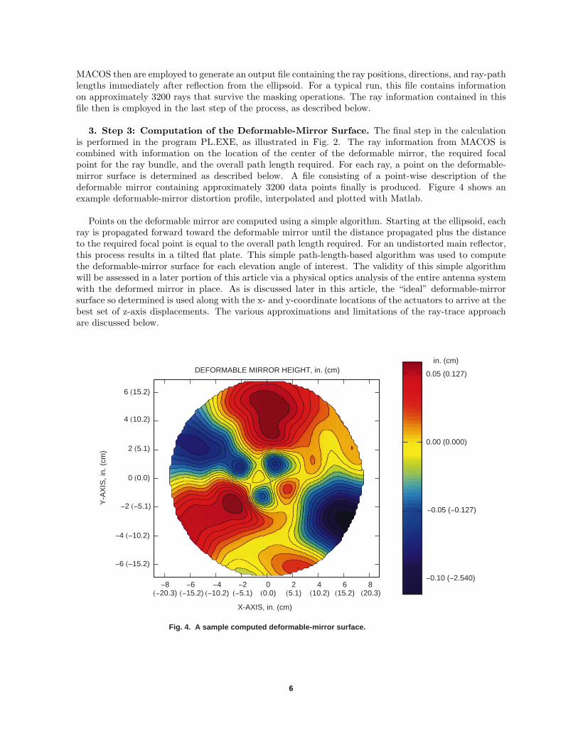
3. Step 3: Computation of the Deformable-Mirror Surface. The final step in the calculationis performed in the program PL.EXE, as illustrated in Fig. 2. The ray information from MACOS iscombined with information on the location of the center of the deformable mirror, the required focalpoint for the ray bundle, and the overall path length required. For each ray, a point on the deformable-mirror surface is determined as described below. A file consisting of a point-wise description of thedeformable mirror containing approximately 3200 data points finally is produced. Figure 4 shows anexample deformable-mirror distortion profile, interpolated and plotted with Matlab.

Points on the deformable mirror are computed using a simple algorithm. Starting at the ellipsoid, eachray is propagated forward toward the deformable mirror until the distance propagated plus the distanceto the required focal point is equal to the overall path length required. For an undistorted main reflector,this process results in a tilted flat plate. This simple path-length-based algorithm was used to computethe deformable-mirror surface for each elevation angle of interest. The validity of this simple algorithmwill be assessed in a later portion of this article via a physical optics analysis of the entire antenna systemwith the deformed mirror in place. As is discussed later in this article, the “ideal” deformable-mirrorsurface so determined is used along with the x- and y-coordinate locations of the actuators to arrive at thebest set of z-axis displacements. The various approximations and limitations of the ray-trace approachare discussed below.

0.05 (0.127)

0.00 (0.000)

-0.05 (-0.127)

-0.10 (-2.540)-8 -6 -4 -2 0 2 4 6 8

-6 (-15.2)

Fig. 4. A sample computed deformable-mirror surface.

DEFORMABLE MIRROR HEIGHT, in. (cm)in. (cm)

(-20.3) (20.3)(15.2)(10.2)(5.1)(0.0)(-15.2) (-10.2) (-5.1)

X-AXIS, in. (cm)

Y-A

XIS

, in.

(cm

)

-4 (-10.2)

-2 (-5.1)

6 (15.2)

4 (10.2)

2 (5.1)

0 (0.0)

6

4. Discussion of Limitations. A number of limitations in the above design procedure need to bediscussed. One basic limitation is in the decision to ignore diffraction entirely and to use a ray-basedapproach. As was discussed above, the penalty paid for ignoring diffraction is not significant and willbe computed exactly in a later section. Another limitation is that only a finite number of rays are usedto define the mirror surface. This limitation is not significant since the surface described by 3200 rayscontains details not resolvable by the finite number of actuators in the actual deformable mirror.

The most significant limitations involve the description of the reflector surfaces in terms of a finiteZernike series. The main-reflector distortions are described to a level exceeding that required for de-termining the actuator positions. Since the surfaces are shaped rather than being a conventional hy-perbola/parabola, the undistorted main-reflector and subreflector surfaces also are described by a finiteZernike series. A ray trace of the undistorted system reveals that a perfect focus is not achieved usingonly 21 circularly symmetric terms in the representation of the shaped reflectors. The major source oferror is in the representation of the subreflector near its apex. In this region, the slope of the subreflectoris discontinuous due to the presence of the vertex plate. The vertex plate directs rays away from thetricone area in the center of the main reflector. Such a surface is not well described in this region bya finite-length Zernike series. The impact of this limitation in the description of the subreflector is alsosmall, as reflected in the physical optics calculations. In the future, it would be beneficial to investigatemethods for inserting a better model for the undistorted reflectors into MACOS.

B. Perfect, Actual, and Measured Plates

The output of the ray-tracing analysis provides the so-called perfect-plate geometry, the geometry thatwill, in a ray-trace sense, perfectly phase compensate for the distortion. The actual DFP is made upof a thin aluminum sheet backed by 16 actuators (see Fig. 5) whose locations were originally chosen tocompensate for the distortion of the DSN 34-m antenna and do not optimally match the desired shapesthat compensate the 70-m antenna. A computer program does exist (derived from the analysis describedin [5]), however, to predict the actuator displacement values that produce a plate surface that best fitsthe desired perfect-plate geometry. Using the best-fit actuator displacements, the surface shape of theactual DFP can be determined. This is the predicted shape of the actual mirror and is the best thatcan be done with the existing 16 actuators. An example of the process is shown in Fig. 6. Figure 6(a)is the perfect plate geometry and is defined only over the portion of the plate that intercepts the raysreflected from the main reflector. The rays intercept a diameter of only about 18 in. (46 cm), whereasthe actual plate is 27 in. (68.6 cm) in diameter. Figure 6(b) is the predicted shape based upon actuatordisplacements that best fit the desired shape. Figure 6(c) is a measurement of the actual plate geometryand is within 0.010 in. (0.25 mm) rms of the calculated shape.

III. Physical Optics Computational Techniques

The basic analysis technique used is the physical optics program described in [6]. For computationalspeed, the program was converted to run in parallel on the California Institute of Technology exemplarcomputer where, on 128 processors, it runs over 100 times faster than on a 266-MHz Pentium Procomputer.

The undistorted asymmetric 70-m dual-reflector system is approximated by a symmetric system sincea drawing of the subreflector with sufficient accuracy for 32 GHz (Ka-band) was not available. However,based on analysis of similar systems, the error introduced by using a symmetric system instead of theactual asymmetric system should be very small and would not alter the basic conclusions. The main-reflector distortions are modeled by a set of Zernike polynomials derived from the processed holographymaps [3]. The feed patterns are computed using the corrugated feed program and an exact mechanicaldescription of the feed.

7

90

13

14

8

6 5

7

12

110

12

3 4

109

16

15

R10.9 cm

R8.4 cm

R29.2 cm

R24.6 cm

R19.3 cm

45.00 deg

60.00 deg

Fig. 5. DFP actuator locations (looking at the mirror face).

The 16-actuator plate geometry is derived from the ray-based theoretical description (previous section)and a computer program [5] that computes the actual shape based upon actuator locations and a finite-element model of the mechanical plate. The perfect plate uses a smoothed version of the theoreticaldescription.

For various reasons, there were additional approximations used in computing the performance of theDFP. Since, when the initial calculations were performed, the errors in the geometry regarding the positionof the ellipse were not known, the errors in the tilt and location of the ellipse relative to the intendedgeometry are not included. Also, the DFP surfaces used in the experiment were generated assuming theDFP was positioned 30 in. (76.2 cm) from the F2 ellipse focal point, not the actual geometry of 28 in.(71.1 cm). Although these differences will lead to some reductions in the DFP performance, it is expectedthat the error will be small and will not alter the conclusions of the experiment.

IV. Focal Plane Analysis

To provide some insight into the performance of the various systems, the focal fields are displayedfor several conditions. Figure 7 shows the focal plane fields for an undistorted system. It is easy toenvision that a single feed horn with the proper spot size would be optimal for this system. It should benoted that none of the auxiliary rings associated with an Airy pattern are present. They are not presentin the dual-shaped reflector system. Figures 8 through 10 show the focal plane fields are significantlyspread out for the distorted cases over the focal plane region, especially for the 85-deg case. Also shownon the 85-deg-elevation map is an outline of the 7-element array feed. For this case, it is obvious that

8

-38.1 -25.4 -12.7 0.0 12.7 25.4 38.1

X-AXIS, cm

(a)

-38.1

-25.4

-12.7

0.0

12.7

25.4

38.1

Y-A

XIS

, cm

X-AXIS, cm

(b)

X-AXIS, cm

(c)

Fig. 6. Plate geometry for 12.7-deg elevation: (a) perfect, (b) actual, and (c) measured.

-38.1

-25.4

-12.7

0.0

12.7

25.4

38.1

Y-A

XIS

, cm

-38.1 -25.4 -12.7 0.0 12.7 25.4 38.1

-38.1 -25.4 -12.7 0.0 12.7 25.4 38.1-38.1

-25.4

-12.7

0.0

12.7

25.4

38.1

Y-A

XIS

, cm

there is significant spillover past the feed horns, limiting the possible improvement of the current arrayfeed. Figures 11 through 13 show the results at F2 for the case of the 16-actuator plate and the smoothedtheoretical plate. Observe that the focal plane spread has been significantly reduced. Also observe thatthe theoretical plate provides nearly complete compensation.

V. Baseline Efficiency

The baseline efficiency was measured at both the F1 and F2 focal points. At F1, the center feed of theAFCS was used, and, at F2, the standard 22.5-dBi horn was used. See [1] for a complete description ofthe data analysis. Using the expected gain difference between F1 and F2, the data at F2 were referencedto F1 and plotted on the same graph (see Fig. 14). Using the all-elevation-angle holography model ofthe antenna distortion, a complete physical optics analysis was made, predicting antenna performanceversus elevation angle. The computed efficiency is the combination of factors not directly included inthe physical optics program plus the computation of the efficiency due to the modeled geometry andmain-reflector surface shape. The items not directly included in the PO computation are summarizedin Table 1. The most significant term is the projection of the medium-resolution holography rms results

9

-62.3

-28.0

-22.0

-16.0

-10.0-4.0

7.6

5.1

2.5

0.0

-2.5

-5.1

-7.6-7.6 -5.1 -2.5 0.0 2.5 5.1 7.6

X-AXIS, cm

Y-A

XIS

, cm

INTERPOLATED DATADEFINED LEVELSY-COMPONENT

Fig. 7. Focal plane distribution of the undistorted dual-reflector system.

dB

7.6

5.1

2.5

0.0

-2.5

-5.1

-7.6

Y-A

XIS

, cm

-7.6 -5.1 -2.5 0.0 2.5 5.1 7.6-65.2

-28.0-22.0-16.0-10.0

-4.0

X-AXIS, cm


Fig. 8. Focal plane distribution of the dual-reflector system, elevation = 15 deg.

dB

10

7.6

5.1

2.5

0.0

-2.5

-5.1

-7.6-7.6 -5.1 -2.5 0.0 2.5 5.1 7.6

-57.1

-28.0

-22.0

-16.0

-10.0

-4.0

X-AXIS, cm

Y-A

XIS

, cm



dB

12.7

10.2

7.6

0.0

-7.6

-10.2

-12.7-12.7 -7.6 -2.5 2.5 7.6 12.7

-67.6

-28.0

-22.0

-16.0

-10.0-4.0

X-AXIS, cm

Y-A

XIS

, cm



AFS TO SCALE

dB

-5.1

-2.5

5.1

2.5

11

7.6

5.1

2.5

-2.5

-5.1

-7.6

0.0

7.6

5.1

2.5

-2.5

-5.1

-7.6

0.0

-7.6 -5.1 -2.5 0.0 2.5 5.1 7.6

X-AXIS, cm

-7.6 -5.1 -2.5 0.0 2.5 5.1 7.6

X-AXIS, cm

Y-A

XIS

, cm

-63.4

-28.0-22.0-16.0-10.0

-4.0

-70.9

-28.0-22.0-16.0-10.0

-4.0

(a) (b)

Fig. 11. Focal plane distribution at F2, elevation = 15 deg (interpolated data, defined levels, y-component):(a) actual plate and (b) smoothed perfect plate.

dB dB

X-AXIS, cm

-7.6 -5.1 -2.5 0.0 2.5 5.1 7.6

X-AXIS, cm

-7.6 -5.1 -2.5 0.0 2.5 5.1 7.6

7.6

5.1

2.5

-2.5

-5.1

-7.6

0.0

Y-A

XIS

, cm

7.6

5.1

2.5

-2.5

-5.1

-7.6

0.0

-74.5

-28.0-22.0-16.0-10.0

-4.0

(a) (b)

-65.6

-28.0-22.0-16.0-10.0

-4.0


dB dB

to infinite-resolution rms. This is due to the fact that the medium-resolution maps do not contain allthe very high-order random rms distortions, and this additional loss must be accounted for separately.The number is based upon comparison of the rms from measured low, medium and high resolution atthe rigging angle and projecting the curve to infinite-resolution rms. The three-angle holography dataare only medium resolution; hence, it is necessary to include the loss due to the missing very high-orderrandom distortions.

Figure 14 contains two computed differences—the efficiency due to using the Zernike polynomialdescription of the main reflector and the efficiency using the full medium-resolution holography maps. Ascan be seen, there is a significant amount of loss not accounted for by the Zernike polynomial descriptionof the main-reflector surface.

12

-7.6 -5.1 -2.5 0.0 2.5 5.1 7.6

X-AXIS, cm

-7.6 -5.1 -2.5 0.0 2.5 5.1 7.6

X-AXIS, cm

7.6

5.1

2.5

-2.5

-5.1

-7.6

0.0

Y-A

XIS

, cm

7.6

5.1

2.5

-2.5

-5.1

-7.6

0.0

-62.3

-28.0-22.0-16.0-10.0

-4.0

-57.9

-28.0-22.0-16.0-10.0

-4.0

(a) (b)


dB dB

USING ZERNIKEPOLYNOMIALS

USING FULL HOLOGRAPHY

0 15 30 45 60 75 900

10

20

30

40

50

HOLOGRAPHY MEASUREMENTS

AFCSDFP

60

ELEVATION, deg

EF

FIC

IEN

CY

, per

cent

Fig. 14. Predicted and measured baseline performance ofthe 70-m antenna at Ka-band.

VI. Comparison of Computed Versus Measured Results

The computed versus measured results for the array feed at F1 are shown in Fig. 15. The datarepresent the gain improvement obtained by using the seven-element array feed over the power in thecenter element alone. Two cases are shown—one using the Zernike polynomial representation of the maindish and the other using the full holography maps. Even though there is a significant gain differencebetween the Zernike polynomials and the full holography maps (see Fig. 12), there is only a very modestimprovement in the array feed performance. This indicates that the higher-order distortions in the fullholography maps versus the Zernike polynomial description cannot be compensated by the array feed.

13

Table 1. DSS 14 estimated efficiency performanceat Ka-band without compensation (rigging angleapproximately 42 deg).

Item Ka-band

Main reflector dissipative loss 0.9991

Panel leak 0.9975

Panel gap 0.9982

Subreflector dissipative loss 0.9991

Beam squint 0.9954

Subreflector focus 1.0000

Cassegrain VSWR (voltage standing- 0.9990wave ratio) loss

Medium-resolution holography 0.7776rms to infinite

Terms not in PO computation 0.767

0 15 30 45 60 75 900

1

2

3

4

5

ELEVATION, deg

GA

IN, d

B

Fig. 15. Predicted and measured AFCS compensation.



The computed versus measured results for the DFP compensation are shown in Fig. 16. Both the com-puted and measured results represent the difference between the DFP in the flat (uncompensated) andflexed (compensated) modes. Since the derivation of the shape of the DFP used only the Zernike polyno-mial representation of the main-dish distortion, only small differences were expected between calculatedresults with either surface representation.

The computed versus measured results for the combined DFP–AFCS are shown in Fig. 17. Thereare several curves shown on the figure. The lower solid curve is the measured baseline efficiency. Thecalculated results for the combined DFP–AFCS using the full holography maps are shown in circles, andthe calculated results using the Zernike polynomial representation of the surface are shown as triangles.The gain using the Zernike polynomial surface description has been reduced by 3.4 dB to account forthe loss due to the random component of the surface not included in the Zernike polynomial representa-tion of the surface. The measured performance of the combined DFP–AFCS system is shown, but onlydata for lower elevation angles were obtained. Observe that the measured and calculated values agreeto within a few percent. Also observe that the combined system recovers almost all of the gain lost dueto the systematic distortion (represented by the Zernike polynomial description of the surface) but does

14



0 15 30 45 60 75 900

1

2

3

4

5

ELEVATION, deg

GA

IN, d

B

Fig. 16. Predicted and measured DFP compensation(actual plate).

USING FULL HOLOGRAPHYFOR COMBINED DFP-AFCSUSING FULL HOLOGRAPHYWITH PERFECT PLATEWITHOUT AFCSAFCS + DFP MEASUREDKa-BAND MEASURED

0 20 40 60 80

ELEVATION, deg

EF

FIC

IEN

CY

Fig. 17. Predicted and measured compensation withthe combined DFP-AFCS (70-m antenna efficiency atKa-band).

0.40

0.45

0.35

0.30

0.25

0.20

0.15

0.10

0.05

0.00

not recover the random component of the surface distortion (the 3.4-dB difference between the Zernikepolynomial and the full holography maps). It is anticipated that a majority of the random componentwill be recovered by resetting the main reflector.

Also shown in Fig. 17 is the expected performance if a so-called “perfect DFP” were used. A perfectDFP means that the required shape of the plate as determined by the Zernike polynomial expansion ofthe main-reflector surface is replicated exactly. With an improved DFP, it should be possible to get closeto the required surface and produce performance close to this prediction. Observe that the perfect DFPdoes not recover the random component of the distortion, as this distortion is not even included in itsdetermination.

15

VII. System Characteristics

Each (DFP or AFCS) system has different characteristics, and the intent of this section is to usethe analytical tools to further understand and document these differences. The section will consist of astatement of the characteristic and an explanation or proof of the validity of the statement.

(1) The current analytical model used for the main-reflector shape does not contain all the dis-tortion.

The Zernike polynomial description of the main-reflector surface shape was used to designthe DFP. It is obvious from Fig. 14 that this description of the main-reflector surface shapeis several dB short of the actual loss in the 70-m antenna. Even the full medium holog-raphy description falls 1.15-dB short of the actual losses (see Table 1). A picture of the15-deg elevation-angle surface is shown in Fig. 18. Figure 18(a) shows the Zernike polynomial

Y-A

XIS

, m

-0.25

-0.20

0.00

0.20

cm

(c)

X-AXIS, m

Y-A

XIS

, m

-34.2 -22.8 -11.4 0.0 11.4 22.8 34.2

(a) (b)

X-AXIS, m X-AXIS, m

Fig. 18. The 15-deg elevation-angle main-reflector surface: (a) Zernike polynomial representation(raw data, autolevel on, y-component) (b) full holography (raw data, user-specified levels,y-component), and (c) the difference between the two surfaces (raw data, user-specified levels,y-component).

-0.25

-0.20

0.00

0.20

cm

-0.25

-0.20

0.00

0.20

cm

-34.2

-22.8

-11.4

0.0

11.4

22.8

34.2

-34.2 -22.8 -11.4 0.0 11.4 22.8 34.2-34.2

-22.8

-11.4

0.0

11.4

22.8

34.2

-34.2 -22.8 -11.4 0.0 11.4 22.8 34.2-34.2

-22.8

-11.4

0.0

11.4

22.8

34.2

16

characterization, Fig. 18(b) the full holography representation, and Fig. 18(c) the differencebetween the two surfaces. Observe that this difference is a very random surface and thatneither the AFCS nor the DFP accurately compensates for this random component of thedistortion. This random component can be greatly reduced by resetting the main-reflectorsurface.

(2) The DFP requires an accurate description of the main-reflector surface shape; the AFCS doesnot.

As seen in the earlier description of the design of the DFP, the basic determination of theDFP requires knowledge of the surface. The AFCS uses the measured signals from the feedsto determine the correct combining weights and does not need to know the shape of thesurface to maximize the received signal. However, knowledge of the surface is required forperformance prediction.

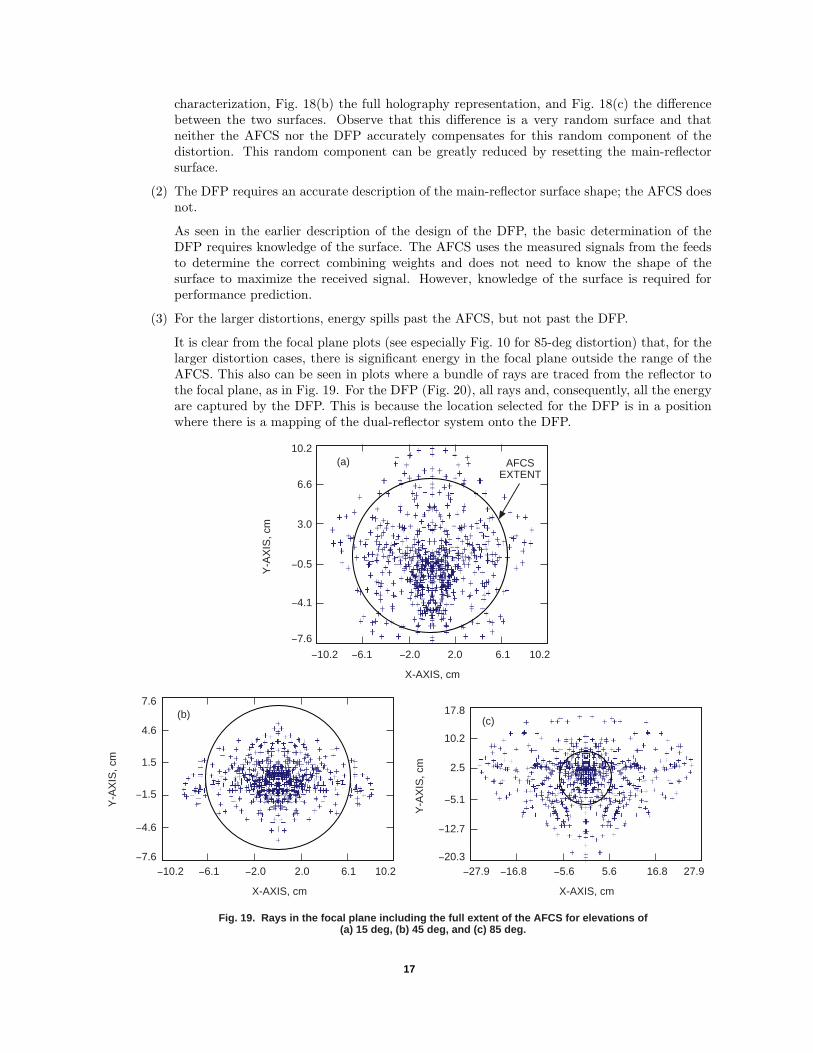
(3) For the larger distortions, energy spills past the AFCS, but not past the DFP.

It is clear from the focal plane plots (see especially Fig. 10 for 85-deg distortion) that, for thelarger distortion cases, there is significant energy in the focal plane outside the range of theAFCS. This also can be seen in plots where a bundle of rays are traced from the reflector tothe focal plane, as in Fig. 19. For the DFP (Fig. 20), all rays and, consequently, all the energyare captured by the DFP. This is because the location selected for the DFP is in a positionwhere there is a mapping of the dual-reflector system onto the DFP.

-10.2 -6.1 -2.0 2.0 6.1 10.2

(c)

-27.9 -16.8 -5.6 5.6 16.8 27.9-20.3

-12.7

-5.1

2.5

17.8

Y-A

XIS

, cm

X-AXIS, cm

10.2

-7.6

-4.6

-1.5

1.5

4.6

7.6

Y-A

XIS

, cm

X-AXIS, cm

(b)

Fig. 19. Rays in the focal plane including the full extent of the AFCS for elevations of(a) 15 deg, (b) 45 deg, and (c) 85 deg.

-7.6

-4.1

-0.5

3.0

6.6

10.2

Y-A

XIS

, cm

-10.2 -6.1 -2.0 2.0 6.1 10.2

(a)

X-AXIS, cm

AFCSEXTENT

17

-20.3

-12.2

-4.1

4.1

12.2

20.3

Y-A

XIS

, cm

-22.9 -13.7 -4.6 4.6 13.7 22.9

(c)

X-AXIS, cm

-20.3

-12.2

-4.1

4.1

12.2

20.3Y

-AX

IS, c

m

-22.9 -13.7 -4.6 4.6 13.7 22.9

(a)

X-AXIS, cm

-20.3

-12.2

-4.1

4.1

12.2

20.3

Y-A

XIS

, cm

-22.9 -13.7 -4.6 4.6 13.7 22.9

(b)

X-AXIS, cm

Fig. 20. Rays hitting the DFP (all rays hit the DFP) for elevations of (a) 15 deg, (b) 45 deg, and (c) 85 deg.The DFP diameter is 68.6 cm, and the area shown is 45.7 cm.

(4) The DFP readjusts the beam to put the peak on the mechanical boresite.

When the dish is distorted because of gravity, the main beam generally is distorted andscanned from the mechanical boresite direction (see Fig. 21(a) for 75-deg elevation). TheDFP both corrects the beam shape and puts the beam peak on the mechanical boresite [seeFig. 21(b)]. The combined gain plot for the AFCS for this case (Fig. 22) shows that the arraydoes not put the beam peak on the mechanical boresite. The combined gain plot of Fig. 22(b)is not a pattern plot but shows the maximum possible gain of the array in each of the givendirections. This plot is useful for determining the optimum gain of the AFCS. However, if theAFCS is used in conjunction with the DFP, since the DFP puts the center-horn peak on themechanical boresite, the combined gain of the AFCS is also on the mechanical boresite (seeFig. 23).

(5) When using the DFP, the monopulse null points in the direction of the main beam peak.

As mentioned earlier, when the dish is distorted, the main beam generally is misshapenand scanned from the mechanical boresite and, in general, the monopulse tracking systemwould not necessarily point in the direction of the main-beam peak. However, as can be seenin Fig. 24, the difference pattern as well as the sum pattern points in the direction of themechanical boresite and, consequently, the sum and difference patterns are co-aligned.

18

Y-A

XIS

, mde

g

23.731.9

40.1

48.2

56.464.5

10.0

6.0

2.0

0.0

-4.0

-8.0

-10.0-10.0 -6.0 -2.0 2.0 6.0 10.0

X-AXIS, mdeg

-45.4

-28.0-24.0-20.0

-4.0

X-AXIS, mdeg

(a) (b)

8.0

4.0

-2.0

-6.0

72.7

80.9

-16.0-12.0

-8.0

0.0

Fig. 21. The DFP readjusts the beam to put the peak on the mechanical boresite (75-deg elevation):(a) no DFP compensation (interpolated data, autolevel on, y-component) and (b) DFP compensation(interpolated data, defined levels, y-component).

10.0

6.0

2.0

0.0

-4.0

-8.0

-10.0

8.0

4.0

-2.0

-6.0

-10.0 -6.0 -2.0 2.0 6.0 10.0

dB dB

Y-A

XIS

, mde

g

35.541.9

48.2

54.6

60.967.3

10.0

6.0

2.0

0.0

-4.0

-8.0

-10.0-10.0 -6.0 -2.0 2.0 6.0 10.0

X-AXIS, mdeg X-AXIS, mdeg

(a) (b)

8.0

4.0

-2.0

-6.0

73.6

80.0

Fig. 22. The AFCS combined gain at 75-deg elevation: (a) center horn (interpolated data, autolevelon, y-component) and (b) combined gain (interpolated data, autolevel on, y-component).

78.2278.82

79.42

80.01

80.6181.21

81.81

82.40

-10.0 -6.0 -2.0 2.0 6.0 10.0

10.0

6.0

2.0

0.0

-4.0

-8.0

-10.0

8.0

4.0

-2.0

-6.0

dB dB

(6) The current AFCS cannot provide vernier beam steering.

In Fig. 25, the maximum gain possible from the AFCS at each point on the −20 to 20 mdeggrid is plotted. An undistorted antenna is assumed for these calculations. As expected, max-imum gain is produced on axis. In addition, nearly identical gain is produced at six otherlocations. These locations correspond to excitations in one of the six outer horns with es-sentially zero amplitude in each of the other horns. For regions between these peaks, themaximum gain falls to more that 10-dB below this peak and drops to nearly zero outsidethese six peaks.

Figure 25 shows that the AFCS provides essentially no electronic scan capability. It is capableof providing seven distinct, non-overlapping beams in the far field. This is expected due to thelarge gain of the individual AFCS elements. Arrays with significant scan capability typically

19

Y-A

XIS

, mde

g

78.2278.82

79.42

80.01

80.61

81.21

10.0

6.0

2.0

0.0

-4.0

-8.0

-10.0-10.0 -6.0 -2.0 2.0 6.0 10.0


(a) (b)

8.0

4.0

-2.0

-6.0

81.8182.40

Fig. 23. The combination of the AFCS plus the DFP puts the beam peak on the mechanical boresiteand provides significantly more gain than either system alone (75-deg elevation): (a) AFCS alone(interpolated data, autolevel on, y-component) and (b) AFCS plus DFP (interpolated data, autolevelon, y-component).

77.378.5

79.6

81.0

82.3

83.5

84.786.0

-10.0 -6.0 -2.0 2.0 6.0 10.0

10.0

6.0

2.0

0.0

-4.0

-8.0

-10.0

8.0

4.0

-2.0

-6.0

dB dB

Y-A

XIS

, mde

g

-45.4

-28.0-24.0-20.0-16.0-12.0

10.0

6.0

2.0

0.0

-4.0

-8.0

-10.0-10.0 -6.0 -2.0 2.0 6.0 10.0


(a) (b)

8.0

4.0

-2.0

-6.0

-8.0

0.0

Fig. 24. The monopulse null points in the direction of the main beam peak (the monopulse feed at75 deg with the DFP flexed): (a) sum (interpolated data, defined levels, y-component) and(b) difference (interpolated data, defined levels, y-component).

-40.8

-28.0-24.0-20.0-16.0-12.0

-8.0

-0.0

-10.0 -6.0 -2.0 2.0 6.0 10.0

10.0

6.0

2.0

0.0

-4.0

-8.0

-10.0

8.0

4.0

-2.0

-6.0

-4.0 -4.0

dB dB

are constructed with element sizes on the order of a wavelength or less and a high ratio ofeffective aperture to physical aperture. The AFCS horns are over four wavelengths in diameterand have highly tapered aperture distributions.

Figure 26 shows the gain of the center feed and the maximum gain available from the AFCSfor scanning in two planes. The x-scan plane corresponds to the favorable situation depictedin the figure, while the y-scan corresponds to the unfavorable situation. For scans of less than5 mdeg around the antenna boresite, the AFCS provides nearly zero additional gain relativeto the center feed alone. In the favorable situation, it recovers almost the total available gain,minus some small scan loss, for a distinct scan angle of approximately 15 mdeg.

20

Y-A

XIS

, mde

g

-28.3-26.0

-22.0

-18.0

-14.0

-10.0

20.0

10.0

0.0

-5.0

-15.0

-20.0


(a) (b)

15.0

5.0

-10.0

-6.0

Fig. 25. AFCS electronic scanning contour plots: (a) far-field combined gain (interpolated data,defined levels, y-component) and (b) far-field center horn (interpolated data, defined levels,y-component).

-48.5

-28.0-24.0-20.0-16.0-12.0

-8.0

0.0-2.0 -4.0

-20.0 -15.0 -10.0 -5.0 0.0 10.05.0 15.0 20.0 -20.0 -15.0-10.0 -5.0 0.0 10.05.0 15.0 20.0

20.0

10.0

0.0

-5.0

-15.0

-20.0

15.0

5.0

-10.0

dB dB

20-10 0 10-20 -15 -5 5 15

AFCS Y-SCAN

AFCS X-SCAN

SINGLE FEED

50

SCAN ANGLE, mdeg

Fig. 26. AFCS electronic scanning: linear cuts.

GA

IN, d

Bi

55

60

65

70

75

80

85

90

(7) Neither the AFCS nor the DFP corrects for small errors in subreflector offset.

The AFCS has the capability to correct for some of this real-time gain loss by electronicallyrecombining the signals in an optimum way. As an example, we consider the simple caseof defocus, electronically compensating for the inability to move the subreflector in responseto real-time effects. For the following calculation, we assume a perfect antenna except for asubreflector defocus.

The situation in the focal plane is depicted in Fig. 27. A simple defocus will increase thespot size in the focal plane of the antenna. For a small defocus, we expect very little of theenergy will spill past the center feed. Because of the defocus, the shape of the distribution

21

will not match the feed distribution exactly, and some of this power will be reflected off thecenter feed. Thus, we do not expect the AFCS to provide excellent compensation for smalldefocus. For a large defocus, significant energy may fall into the outer ring of feeds, and amore significant improvement in gain may be expected from the AFCS.

A simulation of the ability of the AFCS to compensate for defocus was carried out usingphysical optics. The results are presented in Fig. 27. For a subreflector defocus of 0.89 cm,the predicted gain loss is 3.5 dB. The AFCS is capable of recovering 1.0 dB of this loss. Note,however, that for very small motions (0.15 to 0.4 cm) there is almost no improvement fromthe AFCS.

Since there is no adjustment of the DFP for real-time effects like subreflector motion, theDFP offers no correction for such effects.

VIII. Conclusions

Either system provides partial distortion correction, and the combined AFCS–DFP system both ana-lytically and experimentally does an excellent job of distortion compensation. We also have shown that,with an accurate knowledge of the surface, a perfectly shaped DFP alone can provide significant distortioncompensation.

(SMALL DEFOCUS) (LARGE DEFOCUS)

INCIDENT FIELD FOCAL PLANEDISTRIBUTIONS FOR A DISPLACED

SUBREFLECTOR

0.00 0.13 0.25 0.38 0.51 0.63 0.76

-4

-2

-1

0

1

2

0.89-3

DEFOCUS, cm

RE

LAT

IVE

GA

IN, d

B

GAIN LOSS

GAIN LOSS USING AFCSAFCS COMPENSATION

Fig. 27. AFCS defocus compensation.

References

[1] P. Richter, M. Franco, and D. Rochblatt, “Data Analysis and Results of theKa-Band Array Feed Compensation System–Deformable Flat Plate Experimentat DSS 14,” The Telecommunications and Mission Operations Progress Report42-139, July–September 1999, Jet Propulsion Laboratory, Pasadena California,pp. 1–29, November 15, 1999.http://tmo.jpl.nasa.gov/tmo/progress report/42-139/139H.pdf

22

[2] V. Vilnrotter and D. Fort, “Demonstration and Evaluation of the Ka-Band ArrayFeed Compensation System on the 70-Meter Antenna at DSS 14,” The Telecom-munications and Mission Operations Progress Report 42-139, July to September1999, Jet Propulsion Laboratory, Pasadena California, pp. 1–17, November 15,1999.http://tmo.jpl.nasa.gov/tmo/progress report/42-139/139J.pdf

[3] D. J. Rochblatt, D. J. Hoppe, W. A. Imbriale, M. Franco, P. H. Richter,P. M. Withington, and H. J. Jackson, “A Methodology For The Open LoopCalibration Of A Deformable Flat Plate On a 70-Meter Antenna,” AP2000 Mil-lennium Conference on Antennas and Propagation, Davos, Switzerland, April2000.

[4] Modeling and Analysis for Controlled Optical Systems User Manual, Version2.4.1, Jet Propulsion Laboratory, Pasadena, California, April 1, 1997.

[5] R. Bruno, W. Imbriale, M. Moore, and S. Stewart, “Implementation of a GravityCompensation Mirror on a Large Aperture Antenna,” AIAA MultidisciplinaryAnalysis and Optimization Conference, Bellevue, Washington, September 1996.

[6] W. A. Imbriale and R. E. Hodges, “The Linear Phase Triangular Facet Approx-imation in Physical Optics Analysis of Reflector Antennas,” Applied Computa-tional Electromagnetic Society, vol. 6, no. 2, pp. 74–85, Winter 1991.

23

computational methods and theoretical results for the ka

Documents