tstc lectures: theoretical & computational...
TRANSCRIPT

R. Hernandez @ Georgia Tech
TSTC Lectures:
Theoretical & Computational
Chemistry
Rigoberto Hernandez
May 2009, Lecture #3 Statistical Mechanics: Nonequilibrium Systems

R. Hernandez @ Georgia Tech
TSTC Lecture #3
July '09
Statistical Mechanics 2
Major Concepts, Part IV •! Review:
–! Fluid Structure
•! Gas, liquid, solid, …
•! Radial distribution function, g(r)
–! Potential of Mean Force
–! Classical Determination of g(r):
•! Integral Equation Theories
•! Molecular Dynamics
•! Monte Carlo
•! Scattering experiments (e.g., x-ray, or SANS)
•! Renormalization Group Theory
•! Coarse Graining

R. Hernandez @ Georgia Tech
TSTC Lecture #3
July '09
Statistical Mechanics
Renormalization Group (RG) Theory, I
–! Ken G. Wilson, 1982 Nobel Prize
–! Ising Model as example…
•! Each transformation consists of two steps: –! Decimate (remove particles)
–! Renormalize (rescale distances)
•! Group structure: –! When transformations are exact (e.g., in 1D Ising),
obtain an exact group, and an exact theory
–! When transformations are approximate (e.g. in 2D Ising), obtain a semigroup, and the predicted Tc is only as good as the approximation.
•! RG also gives critical exponents, and some observables
3

R. Hernandez @ Georgia Tech
TSTC Lecture #3
July '09
Statistical Mechanics
Renormalization Group Theory, II •! The transformation involves two steps:
–! Decimate e-!H/Q (integrate/sum over chosen variables) !! In Ising Model, this means remove alternating spins
"! Rescale N/2 to N (i.e., L/2 to L)
–! So H (R, !; {p}) " F(2)(R, !(2); {p(2)})
•! At each iteration, you do the same transformation –! F(n)(R, !(n); {p(n)}) " F(n+1)(R, !(n+1); {p(n+1)})
–! If F(n) and F(n+1) have the same structure, •! RG is then exact, and you have a group (with invertability)
•! The system is the same (at all length scales) at fixed points of the map, i.e. when !(n) = !(n+1) and {p(n)} = {p(n+1)}
–! If not, then you must approximate •! F(n+1)(R, !(n+1); {p(n+1)}) ! F(n)(R, !(n+1); {p(n+1)})
–! And hope for the best ?!
4

R. Hernandez @ Georgia Tech
TSTC Lecture #3
July '09
Statistical Mechanics
Renormalization Group Theory, III •! In 1D Spin Ising System:
–! F(2)(R, !(2); {p(2)}) = H (R, !(2); {p(2)})
–! So you get an exact group
–! The only fixed point is at !=# (T=0)
–! Hence RG correctly predicts no Critical point!
•! In 2D Spin Ising System, Zeroth Order Semigroup: –! F(2)(R, !(2); {p(2)}) " H (R, !(2); {p(2)})
–! What if you just leave out the terms that are not nearest neighbor?
•! The structure of F(n)(R, !(n); {p(n)}) is exactly that of a separable product of two 1D Spin Ising systems
•! Incorrectly predicts no Tc!
5

R. Hernandez @ Georgia Tech
TSTC Lecture #3
July '09
Statistical Mechanics
Renormalization Group Theory, IV •! In 2D Spin Ising System, Next Order Semigroup:
–! F(2)(R, !(2); {p(2)}) " H (R, !(2); {p(2)})
–! Now recognize that F(2)(R, !(2); {p(2)}) has terms involving: (Migdal-Kadanoff Transformation)
•! Nearest neighbor, next-nearest neighbor and a 4-point term
•! Let F(2)(R, !(2); {p(2)}) ! F’(2)(R, !(2); {p(2)}), where the latter includes only NN and next-NN terms
–! Repeat the renormalization, i.e., !! Decimate
"! Rescale
#! Migdal-Kadanoff (removing everything but NN and next NN)
–! Critical point(s) at the fixed points of:
•! F(n)(R, !(n); {p(n)}) " F(n+1)(R, !(n+1); {p(n+1)}) for n>2
•! There now exists a nontrivial fixed point, Tc, but it’s not exact… WHY?
6
R. Hernandez @ Georgia Tech
TSTC Lecture #3
July '09
Statistical Mechanics 7
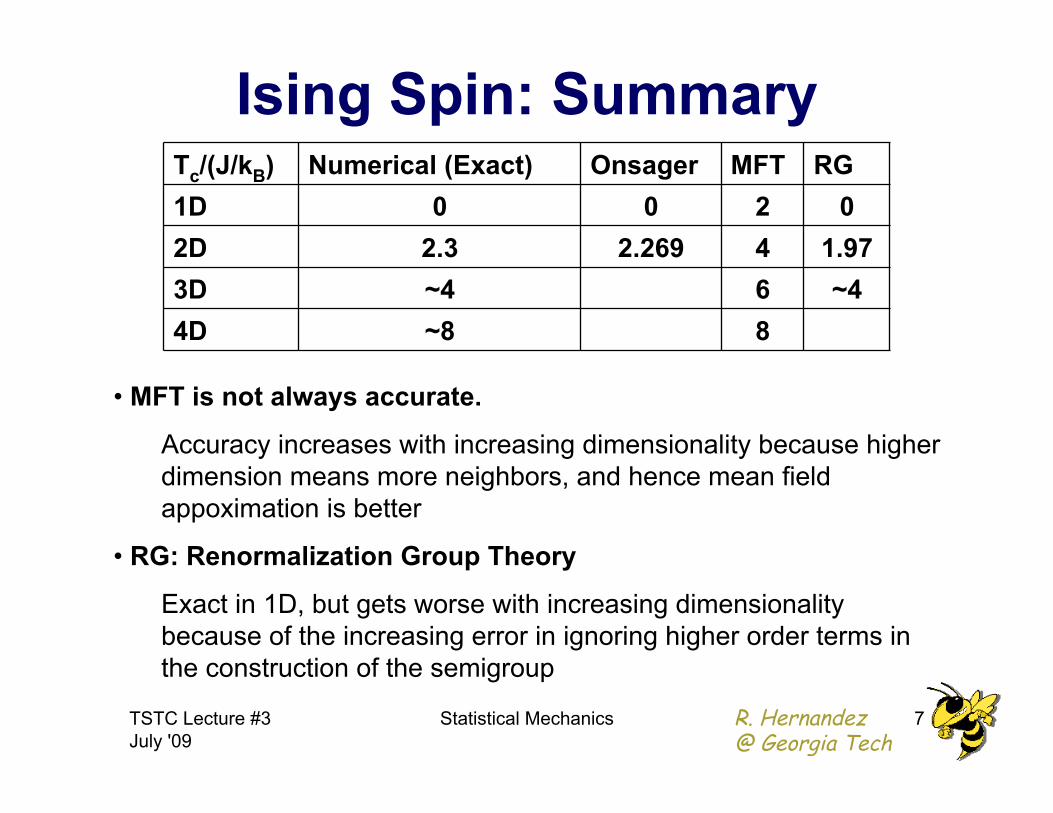
Tc/(J/kB) Numerical (Exact) Onsager MFT RG
1D 0 0 2 0
2D 2.3 2.269 4 1.97
3D ~4 6 ~4
4D ~8 8
•! MFT is not always accurate.
Accuracy increases with increasing dimensionality because higher
dimension means more neighbors, and hence mean field
appoximation is better
•! RG: Renormalization Group Theory
Exact in 1D, but gets worse with increasing dimensionality
because of the increasing error in ignoring higher order terms in
the construction of the semigroup
Ising Spin: Summary
R. Hernandez @ Georgia Tech
TSTC Lecture #3
July '09
Statistical Mechanics 8
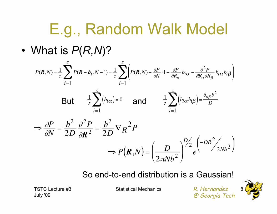
E.g., Random Walk Model
•! What is P(R,N)?
!
P(R,N) = 1z
P(R " bi ,N "1)
i=1
z
# = 1z
P(R,N)" $P$N
%1" $P$R&
bi& " $ 2P$R&$R'
bi&bi'(
) *
+
, -
i=1
z
#
!
1
zbi"( ) = 0
i=1
z
#
!
1
zbi"bi#( ) =
i=1
z
$ %"# b2
DBut and
!
" #P#N
= b2
2D
# 2P
#R2= b
2
2D$R
2P
!
" P R,N( ) = D
2#Nb2$
% &
'
( )
D2
e
*DR2
2Nb2
$ % & '
( )
So end-to-end distribution is a Gaussian!

R. Hernandez @ Georgia Tech
TSTC Lecture #3
July '09
Statistical Mechanics 9
Gaussian Chains •! Take P(R,N) from RW model to describe a
segment…
!
P R,N( ) = D
2"Nb2#
$ %
&
' (
D2
e
)DR2
2Nb2
# $ % &
' (
!
P r ,N( ) = D
2"b2#
$ %
&
' (
D2
e
)Dr2
2b2
# $ % &
' (
!
P Rn{ }( ) = P Rn " Rn"1( )n=1
N
# = D
2$b2%
& '
(
) *
ND2
exp " D
2b2
rn( )2
n=1
N
+%
&
' ' '
(
)
* * *
!
P Rn{ }( )" exp # $k2
Rn # Rn#1( )2
n=1
N
%&
'
( ( (
)
*
+ + +
!
U Rn{ }( ) = k
2Rn " Rn"1( )2
n=1
N
#Bead-Spring model potential:
!
k = D
"b2

R. Hernandez @ Georgia Tech
TSTC Lecture #3
July '09
Statistical Mechanics 10
Radius of Gyration •! A measure of “size” or “volume”
!
RG " mnRn
n=1
N
# mn
n=1
N
#$
% &
'
( ) = 1
NRn
n=1
N
# assuming equal masses
!
Rg2
= 1N
Rn" RG( )
2
n=1
N
# = 1
2N2 R
n" R
m( )2
m ,n
#
!
Rg
2= b
2
2N 2 n "mm ,n
# $ b2
N2 dn
0
N
% dm 0
n
% n "m( ) = 16Nb
2 = 16R
2
For Gaussian chains…
!
Rn " Rm( )2 = n "m b2
R. Hernandez @ Georgia Tech
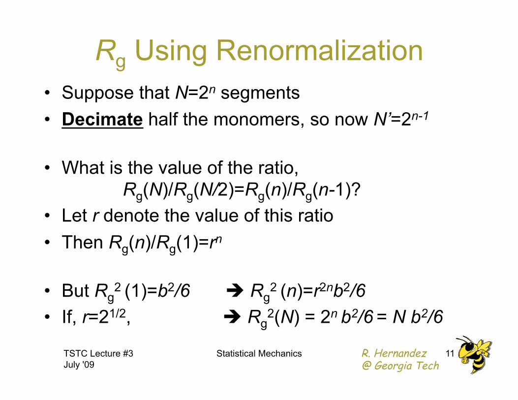
Rg Using Renormalization
•! Suppose that N=2n segments
•! Decimate half the monomers, so now N’=2n-1
•! What is the value of the ratio,
Rg(N)/Rg(N/2)=Rg(n)/Rg(n-1)?
•! Let r denote the value of this ratio
•! Then Rg(n)/Rg(1)=rn
•! But Rg2 (1)=b2/6 ! Rg
2 (n)=r2nb2/6
•! If, r=21/2, ! Rg2(N) = 2n b2/6 = N b2/6
TSTC Lecture #3
July '09
Statistical Mechanics 11

R. Hernandez @ Georgia Tech
E.g., Coarse-Graining
•! Strategy: –! Remove (decimate) some number of degrees of freedom (the
fine-grained variables) by integrating out the others
–! This leads to a reversible work function
–! Use this PMF as the potential in the e.o.m. for the coarse-grained
variables
•! Implications? –! Timescales are too fast!
•! Add dissipation
•! Rescale times
–! Lose information about fine-grained variables
–! Is the PMF reducible to a sum of two-body terms?
–! Can one construct transferable coarse-grained potentials?
TSTC Lecture #3
July '09
Statistical Mechanics 12
“Coarse-Graining of Condensed Phase and Biomolecular Systems,” G. A. Voth, Editor (CRC Press/Taylor and
Francis Group, Boca Raton, FL, 2009).

R. Hernandez @ Georgia Tech
TSTC Lecture #3
July '09
Statistical Mechanics 13
Major Concepts, Part V •! Nonequilibrium Dynamics
–! Correlation Functions
–! Langevin & Fokker-Planck Equations
•! Chemical Kinetics & Rates
–! Kramers Turnover
–! Transition Path Ensemble (Chandler & others)
–! Moving TST (Uzer, Hernandez & others)

R. Hernandez @ Georgia Tech
Nonequilibrium Dynamics •! Far-from-equilibrium, systems are different!
–! Doesn’t the solvent average it all out???
•! Zwanzig’s Topics:
–! Brownian Motion & Langevin Equations
–! Fokker-Planck Equations
–! Master Equations
–! Reaction Rates & Kinetics
–! Classical vs. Quantum Dynamics
–! Linear Response Theory
•! Use thermodynamic quantities to predict Non-Eq
–! Nonlinearity
TSTC Lecture #3
July '09
Statistical Mechanics 14
See, e.g., R. Zwanzig, Nonequilibrium Statistical Mechanics (Oxford University Press, 2001)
R. Hernandez @ Georgia Tech
Time Dependent Correlation Functions
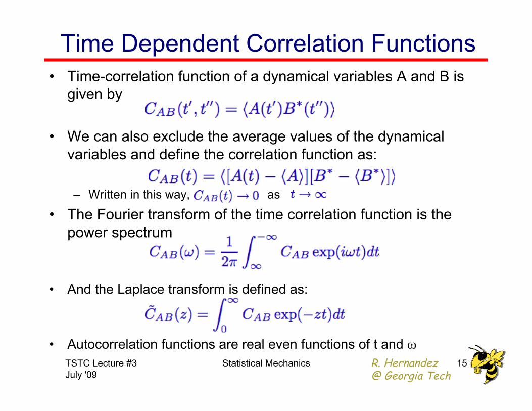
•! Time-correlation function of a dynamical variables A and B is
given by
•! We can also exclude the average values of the dynamical
variables and define the correlation function as:
–! Written in this way, as
•! The Fourier transform of the time correlation function is the
power spectrum
•! And the Laplace transform is defined as:
•! Autocorrelation functions are real even functions of t and !
TSTC Lecture #3
July '09
15 Statistical Mechanics

R. Hernandez @ Georgia Tech
Louisville Operator and Dynamical Variables
•! A is some dynamical variable dependent upon coordinates and momenta
•! Following equation propagates A in time:
–! where L is the Louisville operator [note {A,B} is the Poisson Bracket]
•! For two dynamical variables A and B, inner product give correlation function.
TSTC Lecture #3
July '09
16 Statistical Mechanics

R. Hernandez @ Georgia Tech
Time Dependent Correlation Functions
•! Provide a quantitative description of the dynamics in
liquids
•! Power spectrum is what is measured by many
spectroscopic techniques.
•! Linear transport coefficients of hydrodynamics are
related to time integrals of time dependent correlation
functions.
Why are time dependent correlations functions important?
TSTC Lecture #3
July '09
17 Statistical Mechanics

R. Hernandez @ Georgia Tech
•! Suppose:
•! Then:
•! Why does linear response work?
•! When does linear response not work?
•! What does <A(t)> mean?
TSTC Lecture #3
July '09
Statistical Mechanics 18
Linear Response Theory
!
A(t,x,") :: observable,
x :: internal variable
" :: external variable
!
A(t,x,"#) = "A(t,x,#) for small #
!
A(t,x + "x,#) = A(t,x,#) + $A(t,x,#) % "x for small "x
!
"A(t,#) $ #% &A(t)&A(0)

R. Hernandez @ Georgia Tech
Correlation Functions •!
•! The time correlation function is:
•! The diffusion equation:
•! The diffusion constant is:
TSTC Lecture #3
July '09
Statistical Mechanics 19
R. Hernandez @ Georgia Tech
TSTC Lecture #3
July '09
Statistical Mechanics 20
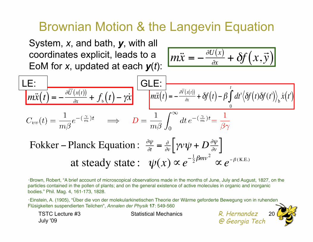
!
m˙ ̇ x = "#U x( )#x
+ $f x,! y ( )
!
m˙ ̇ x t( ) = "#V x t( )( )
#x+ $f t( ) "% dt
0
t
& ' $f t)$f (t'( )b
˙ x t '( )
Brownian Motion & the Langevin Equation
!
m˙ ̇ x t( ) = "#U x t( )( )
#x+ f
bt( ) " $˙ x
System, x, and bath, y, with all
coordinates explicit, leads to a
EoM for x, updated at each y(t):
LE: GLE:
!
Fokker "Planck Equation : #$
#t= #
#v%v$ + D
#$
#v[ ]
!
at steady state : "(x)#e$ 1
2%mv 2
#e$% ( K.E.)
$Brown, Robert, “A brief account of microscopical observations made in the months of June, July and August, 1827, on the particles contained in the pollen of plants; and on the general existence of active molecules in organic and inorganic
bodies.” Phil. Mag. 4, 161-173, 1828. "
$Einstein, A. (1905), “Über die von der molekularkinetischen Theorie der Wärme geforderte Bewegung von in ruhenden
Flüsigkeiten suspendierten Teilchen", Annalen der Physik 17: 549-560"

R. Hernandez @ Georgia Tech
TSTC Lecture #3
July '09
Statistical Mechanics 21
Chemical Kinetics
•! Simple Kinetics—Phenomenology
–!Master Equation
–!Detailed Balance
–!
•! Microscopic Rate Formula
–!Relaxation time
–!Plateau or saddle time (Chandler) !
E.g. : apparent rate for isomerization : " rxn#1
= kAB + kBA

R. Hernandez @ Georgia Tech
Rates
•! The rate is:
–! k(0) is the transition state theory rate
–! After an initial relaxation, k(t) plateaus (Chandler):
•! the plateau or saddle time: ts
•! k(ts) is the rate (and it satisfies the TST Variational Principle)
–! After a further relaxation, k(t) relaxes to 0
•! Other rate formulas:
–! Miller’s flux-flux correlation function
–! Langer’s Im F
TSTC Lecture #3
July '09
Statistical Mechanics 22
!
E.g., in the apparent rate for isomerization : "rxn
#1= k
AB+ k
BA

R. Hernandez @ Georgia Tech
(Marcus: Science 256 (1992) 1523)
Transition State Theory •!Objective: •! Calculate reaction rates
•! Obtain insight on reaction mechanism
•!Eyring, Wigner, Others.. 1.!Existence of Born-Oppenheimer V(x)
2.!Classical nuclear motions
3.!No dynamical recrossings of TST
•!Keck,Marcus,Miller,Truhlar, Others... •! Extend to phase space
•! Variational Transition State Theory
•! Formal reaction rate formulas
•!Pechukas, Pollak... •! PODS—2-Dimensional non-recrossing DS
•!Full-Dimensional Non-Recrossing Surfaces •! Miller, Hernandez developed good action-angle variables at
the TS using CVPT/Lie PT to construct semiclassical rates
•! Jaffé, Uzer, Wiggins, Berry, Others... extended to NHIM’s,
etc
TSTC Lecture #3
July '09
23 Statistical Mechanics
R. Hernandez @ Georgia Tech
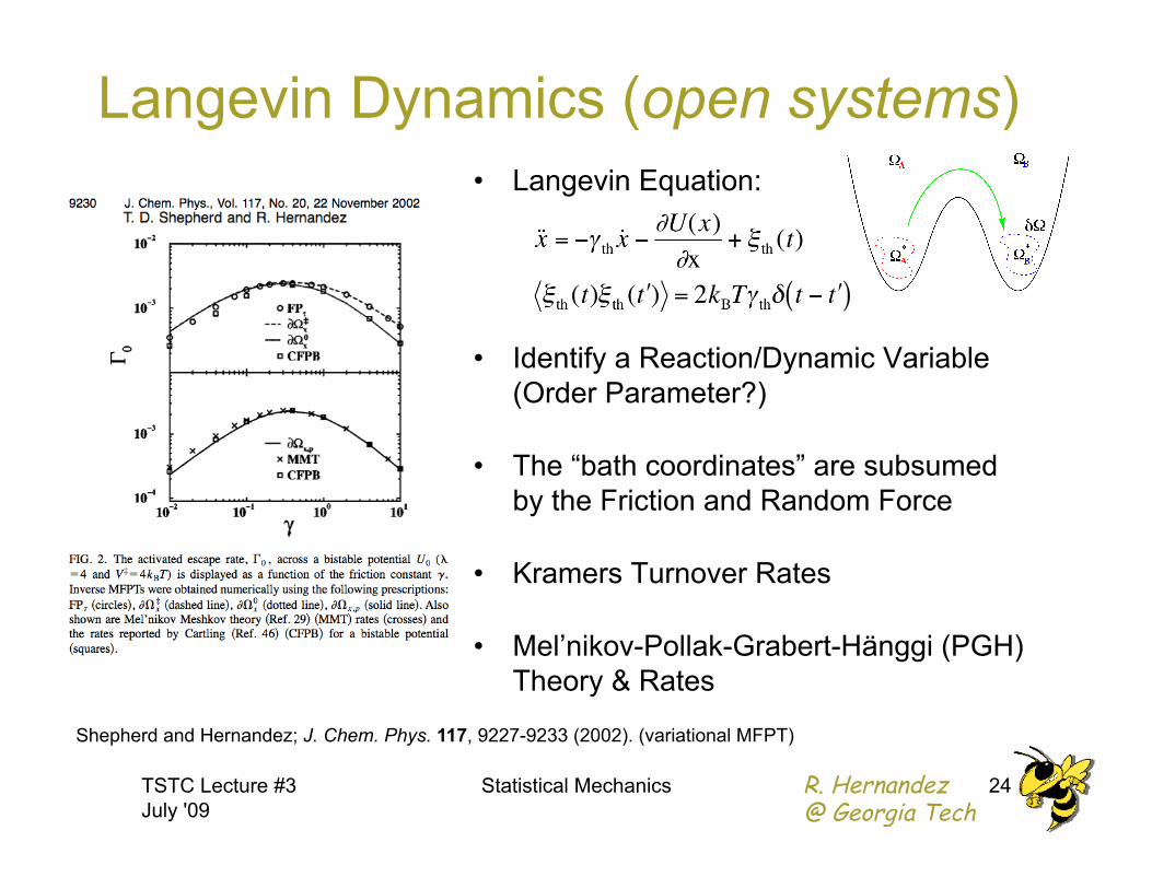
Langevin Dynamics (open systems)
•! Langevin Equation:
•! Identify a Reaction/Dynamic Variable
(Order Parameter?)
•! The “bath coordinates” are subsumed
by the Friction and Random Force
•! Kramers Turnover Rates
•! Mel’nikov-Pollak-Grabert-Hänggi (PGH)
Theory & Rates
Shepherd and Hernandez; J. Chem. Phys. 117, 9227-9233 (2002). (variational MFPT)
TSTC Lecture #3
July '09
24 Statistical Mechanics

R. Hernandez @ Georgia Tech
•! Calculate exact Rates:
–! Reactive Flux as a
function of pressure
–! Convert abscissa to
microscopic friction
•! PGH (TST-like) Rates
–! Construct Langevin Eq.
–! Need PMF
–! Need Friction Kernel
•! Compare Rates García-Müller, Borondo, Hernandez and Benito; Phys. Rev. Let. 101, 178302 (2008)
LiCN in Ar bath
(low P and high T)
TSTC Lecture #3
July '09
25 Statistical Mechanics
Kramer’s Turnover in LiCN
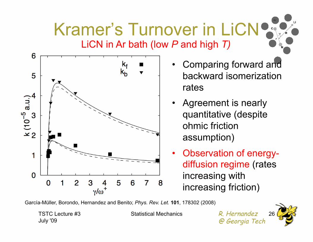
R. Hernandez @ Georgia Tech
•! Comparing forward and
backward isomerization
rates
•! Agreement is nearly
quantitative (despite
ohmic friction
assumption)
•! Observation of energy-diffusion regime (rates
increasing with
increasing friction)
Kramer’s Turnover in LiCN
García-Müller, Borondo, Hernandez and Benito; Phys. Rev. Let. 101, 178302 (2008)
LiCN in Ar bath (low P and high T)
TSTC Lecture #3
July '09
26 Statistical Mechanics

R. Hernandez @ Georgia Tech
Reactions with noise Langevin equation:
We will find a time-dependent non-recrossing dividing surface.
deterministic
potential mean force
(PMF)
damping white noise
TSTC Lecture #3
July '09
27 Statistical Mechanics

R. Hernandez @ Georgia Tech
Decoupling from the noise
Choose trajectory
that never leaves the transition region
as the “moving saddle point”
! w.r.t, Relative coordinate:
the E.o.M are noiseless
! unique stochastic Transition State Trajectory
TSTC Lecture #3
July '09
28 Statistical Mechanics

R. Hernandez @ Georgia Tech
Construction of the TS trajectory Rewrite Langevin equation in phase space,
Scalar equations decouple when A is diagonalized
(eigenvalues !"#):
General solution:
! TS trajectory is given as an explicit function of the noise.
Set c!j=0 so as to keep x!j(t) finite for t"±!"
TSTC Lecture #3
July '09
29 Statistical Mechanics
R. Hernandez @ Georgia Tech
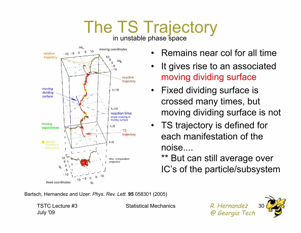
The TS Trajectory
•! Remains near col for all time
•! It gives rise to an associated
moving dividing surface
•! Fixed dividing surface is
crossed many times, but
moving dividing surface is not
•! TS trajectory is defined for
each manifestation of the
noise.... ** But can still average over
IC’s of the particle/subsystem
Bartsch, Hernandez and Uzer: Phys. Rev. Lett. 95 058301 (2005)
in unstable phase space
TSTC Lecture #3
July '09
30 Statistical Mechanics

R. Hernandez @ Georgia Tech
An arbitrary trajectory in configuration space
TS trajectory reactive trajectory
Bartsch, Hernandez and Uzer: Phys. Rev. Lett. 95 058301 (2005) Bartsch, Uzer and Hernandez: J. Chem. Phys. 123 204102 (2005)
TSTC Lecture #3
July '09
31 Statistical Mechanics

R. Hernandez @ Georgia Tech
Statistics of the TS Trajectory •! The distribution of the TS trajectory is stationary.
•! Components are Gaussian distributed with zero mean.
•! Time-correlation functions are known explicitly, e.g.
TSTC Lecture #3
July '09
32 Statistical Mechanics

R. Hernandez @ Georgia Tech
Great, you have a non-
recrossing (moving TS)
dividing surface,
So WHAT?
!! Dynamics can be replaced by GEOMETRY
!! Calculate Rates
!! Obtain Mechanisms
TSTC Lecture #3
July '09
33 Statistical Mechanics

R. Hernandez @ Georgia Tech
Phase Space View of Reaction
In the harmonic approximation, the reaction coordinate and transverse degrees of freedom decouple.
The geometric structures persist even in strongly coupled systems: Normally Hyperbolic Invariant manifolds (NHIM)
TSTC Lecture #3
July '09
34 Statistical Mechanics

R. Hernandez @ Georgia Tech
The barrier ensemble
Sample trajectories in the Transition State region
•! located at fixed “TS” qreact=0
•! Boltzmann-distributed in
bath coordinates and in velocities
Reactive part of the ensemble
is known a priori.
For each trajectory, a unique reaction
time (or “First Passage time” to reach
the moving TS) can be defined.
Averaging over many trajectories
TSTC Lecture #3
July '09
35 Statistical Mechanics

R. Hernandez @ Georgia Tech
Reaction probabilities (Committors)
Reaction probabilities for each
point in phase space:
In particular: The Stochastic Separatrices have been identified
TSTC Lecture #3
July '09
36 Statistical Mechanics

R. Hernandez @ Georgia Tech
Identifying Reactive Trajectories For a fixed instance of the noise
•! sample initial conditions from the Barrier Ensemble
•! propagate forward and backward in time for a time Tint
•! identify reactive trajectories
Reaction probablilities obtained
from moving surface converge
•! monotonically
•! faster than with fixed surface
a priori probabilities are
reproduced asymptotically.
Bartsch, Uzer, Moix and Hernandez; J. Chem. Phys. 124, 244310 (2006).
TSTC Lecture #3
July '09
37 Statistical Mechanics
R. Hernandez @ Georgia Tech
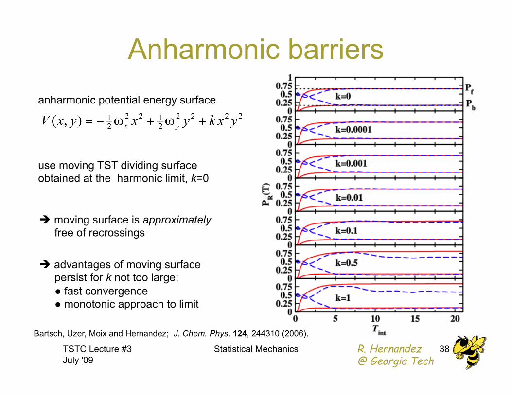
Anharmonic barriers
anharmonic potential energy surface
use moving TST dividing surface
obtained at the harmonic limit, k=0
! moving surface is approximately
free of recrossings
!! advantages of moving surface
persist for k not too large:
# fast convergence
# monotonic approach to limit
Bartsch, Uzer, Moix and Hernandez; J. Chem. Phys. 124, 244310 (2006).
TSTC Lecture #3
July '09
38 Statistical Mechanics

R. Hernandez @ Georgia Tech
Anharmonic Barriers
•! Identifying non-recrossing
trajectories vs. time at
increasing anharmonicity
•! Fixed surface does poorly
even for small
anharmonicity
•! Moving surface (obtained
from harmonic reference!)
does well up to very large
anharmonicity
Moving
Surface
Fixed
Surface
Is the approximate moving TS DS recrossing free?
TSTC Lecture #3
July '09
39 Statistical Mechanics
R. Hernandez @ Georgia Tech
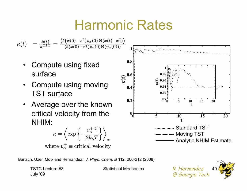
Harmonic Rates
•! Compute using fixed
surface
•! Compute using moving
TST surface
•! Average over the known
critical velocity from the NHIM:
Standard TST
Moving TST
Analytic NHIM Estimate
Bartsch, Uzer, Moix and Hernandez; J. Phys. Chem. B 112, 206-212 (2008)
TSTC Lecture #3
July '09
40 Statistical Mechanics

R. Hernandez @ Georgia Tech
Anharmonic Rates
•! Compute
using fixed
surface
•! Compute
using moving
TST surface Standard TST
Moving TST Note: Change of Lines!
Bartsch, Uzer, Moix and Hernandez; J. Phys. Chem. B 112, 206-212 (2008)
TSTC Lecture #3
July '09
41 Statistical Mechanics

R. Hernandez @ Georgia Tech
•! “Finding Transition Pathways in
Complex Systems: Throwing
Ropes Over Rough Mountain
Passes, In The Dark”
•! Strategy:
–! Find a path between A & B
–! Each trial path is a perturbation of
given path
–! Accept, if it connects A &B
–! Sample over the Path Ensemble!
TSTC Lecture #3
July '09
Statistical Mechanics 42
From Chandler:
http://gold.cchem.berkeley.edu/
research_path.html
Bolhuis, P. G., D. Chandler, C. Dellago, and P. Geissler, Ann. Rev. of Phys. Chem., 59, 291-318 (2002)
C. Dellago, P. G. Bolhuis and P. L. Geissler, "Transition Path Sampling", Advances in Chemical Physics,
123, 1-78 (2002)
Transition Path Ensemble

R. Hernandez @ Georgia Tech
TSTC Lecture #3
July '09
Statistical Mechanics 43
Other Topics, Part VI •! Mode Coupling Theory
–! Wolfgang Götze
–! Matthias Fuchs
–! David Reichmann
•! Fluctuation Theorems
–! Giovanni Gallavotti & E. G. D. Cohen
–! Denis Evans
–! Christopher Jarzynski
–! Jorge Kurchan
•! Accelerated Dynamics
–! Art Voter: hyperdynamics, temperature acceleration, parallel replicas
–! Vijay Pande’s parallel replicas
–! Ron Elber’s Milestone Approach