computation of neutron flux distribution in large …
TRANSCRIPT

COMPUTATION OF NEUTRON
FLUX DISTRIBUTION IN LARGE
NUCLEAR REACTORS VIA
REDUCED ORDER MODELING
by
RAJASEKHAR ANANTHOJU
ENGG01201104012
BHABHA ATOMIC RESEARCH CENTRE, MUMBAI
A thesis submitted to the
Board of Studies in Engineering Sciences
In partial fulfilment of the requirements
for the degree of
DOCTOR OF PHILOSOPHY
of
HOMI BHABHA NATIONAL INSTITUTE
March, 2017


STATEMENT BY AUTHOR
This dissertation has been submitted in partial fulfillment of requirements for an
advanced degree at Homi Bhabha National Institute (HBNI) and is deposited in the
Library to be made available to borrowers under rules of the HBNI.
Brief quotations from this dissertation are allowable without special permission, pro-
vided that accurate acknowledgement of source is made. Requests for permission for
extended quotation from or reproduction of this manuscript in whole or in part may
be granted by the Competent Authority of HBNI when in his or her judgment the
proposed use of the material is in the interests of scholarship. In all other instances,
however, permission must be obtained from the author.
RAJASEKHAR ANANTHOJU

DECLARATION
I, hereby declare that the investigation presented in the thesis has been carried out
by me. The work is original and has not been submitted earlier as a whole or in part
for a degree/diploma at this or any other Institution/University.
RAJASEKHAR ANANTHOJU
List of Publications based on this thesis
Journal Publications
1. Rajasekhar Ananthoju, A. P. Tiwari, and Madhu N. Belur, “A Two-Time-Scale
Approach for Discrete-Time Kalman Filter Design and Application to AHWR
Flux Mapping,” IEEE Transactions on Nuclear Science, Vol. 63 (1), pages 359-
370, 2016.
2. Rajasekhar Ananthoju, A. P. Tiwari, and Madhu N. Belur, “Model Reduction of
AHWR space-time kinetics using balanced truncation,” Annals of Nuclear Energy,
Vol. 102, pages 454-464, 2017.
Conference Publications
1. Rajasekhar. A, A. P. Tiwari, and Madhu N. Belur, “Application of model order
reduction techniques to Space–time kinetics model of AHWR,” In 2015 IEEE
International Conference on Industrial Instrumentation and Control Applications
(ICIC), Pune, India, pages 873-878, 2015.

DEDICATED TO MY FAMILY

ACKNOWLEDGEMENTS
I would like to express my sincere gratitude and respect to my guide Dr. A. P. Tiwari
for giving me an opportunity to work in the area of Nuclear Reactor Dynamics and State
Estimation Theory, and for his invaluable guidance, support and encouragement in all
stages of this research work. Without his vast experience, substantial knowledge in
Reactor Control Theory and insight into the research problem, I would not have been
able to complete this research work.
I would also like to express my sincere gratitude to my co-guide Dr. Madhu N. Belur
for his guidance, support and encouragement during the course work at IIT Bombay
and research work.
I am indebted to my guide and co-guide, for their valuable suggestions and advices in
refining my manuscripts during the initial submission and review process. It has been a
great honour and privilege to me to work under their guidance and to be their student.
I would like to thank Dr. (Smt.) Archana Sharma, Chairman and other members
of the Doctoral Committee, for their valuable comments and suggestions during the
annual progress reviews, oral general comprehensive examination and pre-synopsis pre-
sentations. I would also like to thank Dr. Kallol Roy, former chairman of doctoral
committee .
I wish to express my sincere thanks to Dr. S. R. Shimjith at Reactor Control Systems
Design Section (RCSDS), BARC for valuable technical discussions and inputs. I would
like to thank Shri. A. K. Mishra, Shri S. Subudhi and other members of RCSDS for
their help and support during my research work.
I express my thanks to Shri Y. V. Sagar, my co-researcher and friend for sharing his
material and experience in simulating the mathematical model of the reactor. Thanks
are also due to Shri Jagadish Kota, my friend for his emotional support during my stay
in Mumbai.

I am indebted to Homi Bhabha National Institute, Mumbai for giving me this op-
portunity and to carry out the research work in real time reactor problem at RCSDS,
BARC, Mumbai.
And last but certainly not the least, I would like express my heartfelt thanks to my
family members: Smt. Sandhya Rani, my mother; Shri A. Sesha Chary, my father; Smt.
A. Hema Sireesha, my sister, and Dr. G. H. V. C. Chary, my brother-in-law, for all their
unconditional love, care and support. My parents have always encouraged me towards
higher studies and sacrificed a lot, I am grateful to them. My mother deserves special
mention for her stay with me and having her beside me during this research is the great
source of my motivation and dedication.
RAJASEKHAR ANANTHOJU
Contents
Synopsis i
List of Figures xii
List of Tables xv
Acronyms xvii
Nomenclature xviii
1 Introduction 1
2 Literature Survey 10
2.1 Flux Mapping Algorithms . . . . . . . . . . . . . . . . . . . . . . . . . . 10
2.2 Model Order Reduction . . . . . . . . . . . . . . . . . . . . . . . . . . . 12
2.3 Singular Perturbation Theory and Time–Scale
Methods . . . . . . . . . . . . . . . . . . . . . . . . . . . . . . . . . . . . 17
2.4 Modeling of Nuclear Reactors . . . . . . . . . . . . . . . . . . . . . . . . 20
2.5 State Estimation and Theory of Kalman Filtering . . . . . . . . . . . . . 23
2.5.1 Numerical ill-conditioning in Kalman Filters . . . . . . . . . . . . 25
3 Mathematical modeling of Advanced Heavy Water Reactor 26
3.1 Brief description of the AHWR . . . . . . . . . . . . . . . . . . . . . . . 26
3.2 Space–time kinetics modeling of AHWR . . . . . . . . . . . . . . . . . . 31

Rajasekhar. A: Computation of Neutron Flux Distribution in Large Nuclear Reactorsvia Reduced Order Modeling
3.2.1 Time–dependent core neutronics equations . . . . . . . . . . . . . 33
3.2.2 Formulation of regulating rod reactivity change . . . . . . . . . . 40
3.2.3 Formulation of Xenon reactivity feedback . . . . . . . . . . . . . . 41
3.3 Steady–state Neutron Flux Distribution . . . . . . . . . . . . . . . . . . 41
3.3.1 Homogenization of Interaction Cross-sections . . . . . . . . . . . . 42
3.4 Reconstruction of 3-D Neutron Flux Distribution . . . . . . . . . . . . . 44
3.4.1 Reconstruction of SPND flux . . . . . . . . . . . . . . . . . . . . 45
3.5 Model validation . . . . . . . . . . . . . . . . . . . . . . . . . . . . . . . 47
3.5.1 Case I: Movement of RR in Quadrant–I . . . . . . . . . . . . . . . 48
3.5.2 Case II: Differential Movement of 2 RRs . . . . . . . . . . . . . . 49
3.6 Discussion . . . . . . . . . . . . . . . . . . . . . . . . . . . . . . . . . . . 56
4 Theory of Model Reduction Techniques 57
4.1 Formulation of Model Order Reduction Problem . . . . . . . . . . . . . . 58
4.2 Davison’s Technique . . . . . . . . . . . . . . . . . . . . . . . . . . . . . 59
4.3 Marshall’s Technique . . . . . . . . . . . . . . . . . . . . . . . . . . . . 61
4.4 Singular Perturbation Analysis . . . . . . . . . . . . . . . . . . . . . . . 63
4.4.1 Two-Time-Scale Decomposition of Singularly Perturbed Systems . 65
4.5 Balanced Truncation Method . . . . . . . . . . . . . . . . . . . . . . . . 67
4.5.1 Model decomposition into stable and unstable subsystems . . . . 68
4.5.2 State-Space Balancing Algorithm . . . . . . . . . . . . . . . . . . 70
5 Application of Model Order Reduction Techniques to Space–Time Ki-
netics Model of AHWR 75
5.1 Derivation of Estimation Model . . . . . . . . . . . . . . . . . . . . . . . 76
5.2 Model Order Reduction of AHWR Space–Time Kinetics Model . . . . . . 82
5.2.1 Reduced Model Based on Davison’s Technique . . . . . . . . . . . 83
5.2.2 Reduced Model Based on Marshall’s Technique . . . . . . . . . . 84
5.2.3 Reduced Model Based on Singular Perturbation Analysis . . . . . 84
5.2.4 Reduced Model Based on Balanced Truncation . . . . . . . . . . . 85
5.3 Comparison of Different Reduced Order Models with the Application of
Space-Time Kinetics Model of AHWR . . . . . . . . . . . . . . . . . . . 88
5.4 Discussion . . . . . . . . . . . . . . . . . . . . . . . . . . . . . . . . . . . 92
6 A Two-time-scale approach for Discrete-Time Kalman Filter Design
and application to AHWR Flux Mapping 99
6.1 Discrete-Time Kalman Filter Algorithm . . . . . . . . . . . . . . . . . . 100
6.1.1 Time Update Equations . . . . . . . . . . . . . . . . . . . . . . . 101
6.1.2 Measurement Update Equations . . . . . . . . . . . . . . . . . . . 101
6.2 Two-time-scale approach for Discrete-Time Kalman Filter design . . . . . 102
6.3 Application to AHWR Flux Mapping . . . . . . . . . . . . . . . . . . . . 104
6.4 Computation of Error . . . . . . . . . . . . . . . . . . . . . . . . . . . . . 108
6.4.1 Response of DKF to Non-Zero Initial Condition of Estimation Model109
6.4.2 Movement of Regulating Rods . . . . . . . . . . . . . . . . . . . . 111
6.4.3 Xenon-Induced Oscillations . . . . . . . . . . . . . . . . . . . . . 118
6.5 Discussion . . . . . . . . . . . . . . . . . . . . . . . . . . . . . . . . . . . 121
7 Conclusions and Future Scope 122
References 126
Synopsis
Synopsis
Because of potential for accidents or sabotage at nuclear power plants, the operation
and control of these plants represents a complex problem. Several safety and control
features are engineered at the design stage and operational policies are incorporated to
avoid accidental release of radioactivity to the general population. The problems are
further complicated in case of large nuclear reactors [113].
The current generation modern power reactors are increasing in size to get the benefit
from the economies of generation of electricity. An useful parameter for assessing the
effective size of a reactor is neutron migration length M , a measure of the average
distance travelled by a neutron from its appearance as a fission neutron to its absorption
as a thermal neutron. For a given reactor design, M is determined by the material
composition of the reactor core, primarily the fuel-to-moderator ratio and is essentially
independent of core size R. As the core size increases, the ratio R2/M2 increases,
the migration length becomes a smaller fraction of the reactor core dimension. Thus,
each neutron’s zone of influence becomes a smaller fraction of the core volume, and
the various regions of the core become loosely coupled. Any deliberate attempt to
operate the reactor with flattened radial and axial flux distributions coupled with xenon
poisoning effect leads to complex operational and control problems. The mechanism of
135Xe production and its removal by neutron absorption and radioactive decay are such
that oscillations of thermal flux are induced in large thermal reactors. Such oscillations
induced by 135Xe can broadly be classified into two categories - fundamental mode or
global power oscillations and higher mode or spatial oscillations. Generally speaking,
global power oscillations can be readily noticed and suppressed by control system while
spatial oscillations are not. Here, the global reactor power can remain constant so that
no change in the coolant outlet temperature is effected, the oscillations being in spatial
distribution of power inside the core.
If these oscillations are left uncontrolled, the power density and time rate of change
of power at some locations in the reactor core may exceed the respective design limits.
i
Rajasekhar. A: Computation of Neutron Flux Distribution in Large Nuclear Reactorsvia Reduced Order Modeling
These xenon induced spatial oscillations and subsequent local overpowers pose a poten-
tial threat to the fuel integrity of the reactor. Therefore, the detailed knowledge of axial
and radial flux distribution in the core during the course of their operation is crucial.
Modern reactors have provisions for online spatial control and monitoring of flux or
power distribution during the course of their operation. The time varying neutron flux
distribution is computed by an online Flux Mapping System (FMS), with the help of
flux mapping algorithms. The measurement signals of several in-core flux detectors are
processed to generate the detailed three dimensional flux map, which helps for spatial
control purpose. In CANDU-6 reactors and in Indian 540 MWe Pressurized Heavy
Water Reactors (PHWRs), 102 Vanadium detectors are used for flux mapping, while in
PWRs it is carried out by Rhodium detectors installed in about 45 fuel assemblies. Over
the years, research has been carried out to evolve an efficient flux mapping algorithm
for the improvement of accuracy in flux mapping with less computational effort. Most
of the algorithms existing in the literature are based on three principles, namely the
Flux Synthesis, Internal boundary condition and simultaneous least squares solution of
neutron diffusion and detector response equations.
The most popular and traditional method for flux mapping is known as Flux Synthe-
sis Method (FSM) [46]. It uses the available detector measurements and performs least
squares fit with pre-computed flux modes, determined based on reactivity devices config-
uration. Determination of flux modes requires the knowledge of core configuration and
considerable insight into the reactor operation. There are other synthesis methods such
as Harmonic Synthesis Method (HSM) [95] and Harmonic Expansion Method (HEM)
[133] to improve the accuracy of flux mapping, however the accuracy of reconstruction
depends on selection of the reference case. Selection of a suitable reference case which
reflects the actual core condition results in improvement of the reconstruction accuracy.
During the core configuration changes, the reference case has to be renewed, which can
be a time consuming process.
A Method based on direct online solution of neutron diffusion equations with detector
ii
Synopsis
readings as the internal boundary condition is reported in [52]. A method which obtains
a least squares solution of the core neutronics design equations alongwith the in-core
detector response equations is reported in [47]. Applicability of this least squares method
requires to solve the overdetermined system of equations resulting in the framework of
mapping algorithm. Another approach with the combination of FSM and least squares
method, known as modified flux synthesis method has been proposed for Indian 700
MWe PHWR in [80]. This method takes longer computation time than FSM does [47]
and detector signal uncertainty can also deteriorate the performance of flux mapping
calculations. A common drawback of the aforesaid methods is that they fail to account
for time variation of neutron flux distribution during the reactor operation and the
accuracy might be degraded considerably in presence of uncertainty in the detector
readings.
In contrast to this, model based estimation methods such as the Kalman filter [53],
which infer the system dynamic state on the basis of a sequence of noisy measurements,
offer interesting potential for successful online application. The Kalman filter has re-
ceived a huge interest from the industrial community and has played a key role in many
engineering fields since 70’s, ranging, without being exhaustive, trajectory estimation,
state and parameter estimation for control and diagnosis, data merging, signal pro-
cessing, etc. It is a recursive computational algorithm that processes measurements to
deduce a minimum error estimate of the state of a system by utilizing: knowledge of sys-
tem and measurement dynamics, assumed statistics of system noises and measurement
errors, and initial condition information.
Advanced Heavy Water Reactor (AHWR) [119] is a 920 MW (thermal), vertical,
pressure tube type, heavy water moderated, boiling light water cooled natural circula-
tion reactor being designed in India. The radial dimensions of the core are very large.
Therefore, from neutronic view-point, the behavior tends to be loosely coupled, due to
which a serious situation called ‘flux tilt’ may arise in AHWR followed by an opera-
tional perturbation. These operational perturbations might lead to slow xenon induced
iii
Rajasekhar. A: Computation of Neutron Flux Distribution in Large Nuclear Reactorsvia Reduced Order Modeling
oscillations, which might cause changes in axial and radial flux distribution from the
nominal distribution. Knowledge of any such changes during the reactor operation is
crucial. Therefore, it is necessary to provide online monitoring and control schemes
during the reactor operation. To monitor the core flux distribution, 200 Self Powered
Neutron Detectors (SPNDs) are proposed to be provided at different elevations of the
assembly covering entire AHWR core from top to bottom [1]. An efficient flux mapping
algorithm in AHWR can ensure better reactor regulation and core monitoring, as more
accurate estimates of channel and zonal powers will be available to Reactor Regulating
System (RRS) and Core Monitoring System.
This thesis presents a Discrete-time Kalman filter (DKF) formulation for flux map-
ping in AHWR which is quite different from the existing methods as it can take care
of both time varying phenomena and random errors in the detector readings. For this,
a reasonably accurate mathematical model which represents the time-dependent core
neutronics behaviour of AHWR core is required. A space-time kinetics model with 17
nodes in the core and which exhibits all the essential control related properties and yields
accurate transient response characteristics is utilized for the studies as it is more suitable
for flux distribution studies owing to its simplicity and the structure, thus facilitating
selection of state variables for the system in a straightforward manner. An important
characteristic of the model based on nodal methods is that the order of mathematical
model depends on the number of nodes into which the reactor spatial domain is divided.
A rigorous model with more number of nodes will give good accuracy in designing of
DKF algorithm for flux mapping. However, at the same time, nuclear reactor models
often exhibit simultaneous presence of dynamics of different speeds. Such behavior leads
the mathematical model exhibiting multiple time-scales, which may be susceptible to
numerical ill-conditioning.
The work in this thesis begins with derivation of estimation model for flux mapping
studies in the AHWR. The nonlinear mathematical model (core neutronics and control
rod dynamics equations) is linearized around the steady-state full power operation by
iv

Synopsis
considering a small perturbation in the system and then the equations are cast into
standard state-space form. It is characterized by 80 states, 4 inputs and 200 outputs.
A keen observation of the eigenvalues of the estimation model reveals that they fall into
two distinct clusters. First cluster has 21 eigenvalues consisting of 5 eigenvalues at the
origin and the other 16 eigenvalues ranging from −6.2977× 10⁻² to −5.1852× 10⁻² and
the second one is of 59 eigenvalues ranging from −4.751×10² to −8.4578. This indicates
the presence of two-time-scales in the estimation model. The modern control design and
analysis studies with this model are accompanied by serious numerical ill-conditioning
problems. In this context approximation of high dimensional system by simplified mod-
els or model order reduction is a common procedure in engineering practice. Model
order reduction is defined as the problem of finding a simpler mathematical model for a
complex large-scale system.
The main intent of model order reduction is to preserve the important dynamic
characteristics of the model while certain less important characteristics are ignored. In
the past few decades, several analytical model reduction techniques have been proposed
for the state-space models. Davison [14] proposed one of the first model reduction
technique. The principle of this method is to neglect eigenvalues of the original system
which are farthest from the origin and retain only dominant eigenvalues and hence
the time constants of the original system in the reduced order model. This implies
that the overall behaviour of the reduced-order model will be very similar to that of the
original model, since the contribution of unretained eigenvalues are important only at the
beginning of the response, whereas the eigenvalues retained are important throughout
the whole response. Simultaneously, Marshall [77] developed a technique which preserves
the steady-state of the original system by exciting the modes in the reduced model
differently from those in the original system.
For the mathematical models involving the interaction of slow and fast dynamics,
a method based on decomposition of higher order model into slow and fast systems by
two-time-scale methods and singular perturbation analysis [65] has been proposed for
v
Rajasekhar. A: Computation of Neutron Flux Distribution in Large Nuclear Reactorsvia Reduced Order Modeling
model order reduction. The approach makes use of the standard singularly perturbed
form representation of dynamic systems in which the derivatives of some state variables
are multiplied with a small positive scalar, ε. The model reduction is achieved by setting
ε = 0 and substituting the solution of states whose derivatives were multiplied with ε,
in terms of the other state variables. Essentially the singular perturbation approach to
order reduction can be related to the “dominant mode” techniques which neglect the
high frequency parts and retain low frequency parts of models.
Model order reduction based on the assessment of degree of controllability and ob-
servability has been suggested in [81, 94] which is popularly known as balanced trun-
cation. In order to obtain the original system in balanced form, its basis should be
transformed into another basis where the states which are difficult to reach are simul-
taneously difficult to observe. It can be achieved by simultaneously diagonalizing the
reachability and the observability gramians [70], which are the solutions respectively to
reachability and observability Lyapunov equations. The positive diagonal entries in the
order of decreasing values in the diagonal reachability and observability gramians in the
new basis are called Hankel singular values of the system. The reduced order model
is obtained simply by truncation of the states corresponding to the smallest singular
values. The number of states that can be truncated depends on how accurate the ap-
proximate model is needed. There are some other techniques to obtain the balanced
truncation viz., Schur method [98], balance square root method [132] similar to [81],
however, they differ in the algorithms for obtaining the balancing transformation. The
aforesaid methods can be efficiently applied when the system is asymptotically stable
and minimal, however, for the systems where the stabilization is the major concern their
straightforward application is not possible. Balanced truncation for unstable systems
has also been attempted in [131]. Usually unstable poles cannot be neglected, therefore
model reduction in this situation can be treated by first separating the stable and un-
stable parts of the model and then reducing the order of the stable part using balanced
truncation methods.
vi
Synopsis
For the estimation model of AHWR various model order reduction techniques, viz.,
Davison’s and Marshall’s dominant mode retention techniques; balanced truncation tech-
nique and model decomposition into slow and fast subsystems based on singular per-
turbation analysis, have been applied to obtain a reduced order model from the original
high order model, and results reported in this thesis.
Application of methods based on retention of dominant modes requires diagonaliza-
tion. For the estimation model, it is quite difficult task to get the model into diagonal
form as there are multiple eigenvalues at the origin of the complex s-plane. This is due
to the fact that the model contains slow control rod dynamics. In this thesis, a system-
atic method has been suggested to handle the numerical ill-conditioning occurring in the
computations due to the presence of the slow control rod dynamics by decoupling the
higher order model into very slow and fast models. Model order reduction techniques
based on Davison’s and Marshall’s dominant mode retention are then applied to retain
the slow dynamics. Finally the reduced order model has been formulated by augmenting
the control rod dynamics to the model corresponding to the slow dynamics. Also, it is
essential for model order reduction based on Davison’s and Marshall’s techniques, to
identify the modes to retain and those to truncate/reduce.
The distance between two eigenvalue clusters of the estimation model, computed by
dividing the largest absolute value of the slow (first) group by the smallest absolute
value of the fast (second) group, is ε = 0.0074. This value is small enough to motivate
the use of singular perturbation analysis and two-time-scale based techniques [61, 63].
Therefore it would be possible to decompose the model into a slow subsystem of order
21 and a fast subsystem of order 59, by the application of singular perturbation. For
carrying out this, a regrouping of states variable has been suggested in the thesis.
Finally, comparative study has also been presented in this thesis from the view point
of transient performance between different reduced order models of AHWR, namely,
Davison’s technique, Marshall’s technique, singular perturbation analysis and balanced
truncation by comparing their performances relative to each other and with the original
vii
Rajasekhar. A: Computation of Neutron Flux Distribution in Large Nuclear Reactorsvia Reduced Order Modeling
model. All of these methods are found to be effective, however the overall accuracy in
the approximation using the balanced truncation approach is found to be far superior.
Among these, Davison’s and Marshall’s techniques require diagonalization and bal-
anced truncation technique requires a modal decomposition into unstable and stable
subsystems. Also, it is essential for model order reduction based on Davison’s and Mar-
shall’s techniques, to identify the modes to retain and those to truncate/reduce. In
contrast, singular perturbation techniques require a decomposition of the state-space
systems into fast/slow subsystems using block diagonalization methods. Davison’s and
Marshall’s techniques result into a simplified model that retains the slowly varying dy-
namics while the application of singular perturbation analysis and two-time-scale meth-
ods decompose the model into two subsystems viz., slow and fast, thus providing better
approximation of dynamics of the system. Quite similar to this, application of balanced
truncation yields a reduced model in which both the slow and fast dynamic characteris-
tics are simultaneously retained yielding good accuracy in approximation of high order
model by reduced order model.
The task of flux-mapping in AHWR has been formulated as linear stochastic esti-
mation problem and the solution is obtained by Kalman filtering technique. It utilizes
estimation model and available detector measurements corrupted with white Gaussian
noise. However, direct implementation of the DKF algorithm to this high-order stiff
estimation model is not feasible as the designing procedure is accompanied by serious
numerical ill-condition caused by the simultaneous presence of slow and fast phenom-
ena typically present in a nuclear reactor. In particular, the set of recursive equations
for computation of DKF gains, as a solution to weighted least squares problem, is ill-
conditioned. Consequently, serious numerical difficulties are expected if the DKF gain
matrix is to be computed on the basis of the full order Riccati equation. Fortunately,
this situation can easily be handled by singular perturbation analysis and two-time-scale
methods. This thesis presents a novel technique to address the numerical ill-conditioning
problems in full order design by decoupling the DKF equations according to the order
viii

Synopsis
of the slow and fast subsystems. Finally this technique has been applied for estimation
of detailed mesh, channel and zonal fluxes in the AHWR.
The effectiveness of the Kalman filtering technique for flux mapping has been ex-
amined in three cases. In the first case, decay of non-zero initial condition is observed.
The states of the estimation model are non-zero while the reactor is assumed to be at
steady–state. In the second, the movement of one or multiple Regulating Rods (RRs)
is simulated. Finally in the third case, xenon-induced spatial oscillation is considered.
SPND signals (measurements) were generated under the same transient situations from
a separate set of off-line computations using a 128 node scheme, for the first two cases,
and the 17 node scheme for the third case. Measurement noise of the order of 2 %
has been assumed for each SPND. This noise is equivalent to 2 % random fluctuations
around the full power steady–state value in each detector. DKF based flux mapping
algorithm was processed for the estimation of detailed flux distribution in AHWR for
the respective cases. To characterize the performance of DKF, error analysis has been
carried out to determine the the Root Mean Square (RMS) error and relative error. The
efficacy of the algorithm has been validated from simulations.
The contributions of this thesis are as follows:
1. The monitoring and control of time-varying axial and radial flux distribution in
operational large reactors is a challenging problem. Although several researchers
addressed the flux mapping problem of the other reactors with various advanced
algorithms and methodologies, they have a common disadvantage of failing to take
into account the time variation and loss of accuracy in presence of random errors.
The algorithm suggested in this report is based on Kalman filtering technique
which can take care of both the stated factors.
2. For validation of different techniques of flux mapping, computation results gener-
ated using a high fidelity model is a necessity. Hence, a model based on 128-nodes
in the core of the AHWR resulting into 1168th order is developed.
ix

Rajasekhar. A: Computation of Neutron Flux Distribution in Large Nuclear Reactorsvia Reduced Order Modeling
3. Different approaches of obtaining reduced order models from the original higher
order estimation model of AHWR viz., Davison’s, Marshall’s, singular perturbation
and balanced truncation techniques have been explored to solve the numerical ill-
conditioning in control design and analysis.
4. The concept of application of Kalman filtering theory has been extended to the
near optimal estimation of core flux distribution in AHWR.
5. A novel technique has been suggested based on two-time-scale formulation of
Kalman filtering problem for the time-dependent neutron diffusion equation to
near-optimum estimation of the core flux profile in AHWR.
The conclusions from the work are:
• The proposed DKF algorithm can accurately estimate the time dependent neutron
flux distribution during the typical reactor operating conditions. The degradation
of DKF algorithm accuracy is also very less against the detector random errors.
Therefore, the proposed method can serve an effective alternate to the existing
flux mapping techniques.
• Before deployment in the AHWR, the efficacy of the technique needs to be es-
tablished further and it should be demonstrated using plant data, such as from
PHWRs that it yields improvement in accuracy compared to that resulting from
existing techniques.
• The algorithm should also be assessed from the viewpoint of implementation that
the computations could be performed in real-time using hardware and other re-
sources, suitable for control and instrumentation systems in nuclear reactors.
Possible future extension of the work would be:
• A reduced order Kalman filter can be designed based on the simplified model
obtained from balanced truncation approach for the estimation of core flux distri-
bution in AHWR.
x

Synopsis
• Optimality and availability of DKF based flux mapping algorithm can be verified
under the faults in some of the SPND signals.
xi
List of Figures
3.1 AHWR Core with reactivity devices and ICDH Locations . . . . . . . . . 27
3.2 AHWR core layout (schematic). . . . . . . . . . . . . . . . . . . . . . . . 29
3.3 17 Node scheme of AHWR for (a) the active core region (17 nodes in
core and 8 nodes in side reflector) (b) top reflector region and (c) bottom
reflector region. . . . . . . . . . . . . . . . . . . . . . . . . . . . . . . . . 32
3.4 128 Node scheme. . . . . . . . . . . . . . . . . . . . . . . . . . . . . . . . 39
3.5 SPND in an ICDH surrounded by 8 mesh boxes. . . . . . . . . . . . . . . 46
3.6 Four quadrants in the AHWR core. . . . . . . . . . . . . . . . . . . . . . 47
3.7 Position of RR corresponding to applied control signal. . . . . . . . . . . 49
3.8 Core average flux alongwith error (%) during the transient involving the
movement of RR in Quadrant-I. . . . . . . . . . . . . . . . . . . . . . . . 50
3.9 Average flux in Quadrants I and II during the movement of RR in quad-
rant I. . . . . . . . . . . . . . . . . . . . . . . . . . . . . . . . . . . . . . 51
3.10 Average flux in Quadrants III and IV during the movement of RR in
quadrant I. . . . . . . . . . . . . . . . . . . . . . . . . . . . . . . . . . . 52
3.11 Position of RRs in Quadrant-I and Quadrant-III during the transient
involving differential movement of RRs. . . . . . . . . . . . . . . . . . . . 53
3.12 Core average flux alongwith error (%) during the transient involving dif-
ferential movement of RRs. . . . . . . . . . . . . . . . . . . . . . . . . . . 53
xii
List of Figures
3.13 Average flux in Quadrants I and II during the transient involving differ-
ential movement of RRs. . . . . . . . . . . . . . . . . . . . . . . . . . . . 54
3.14 Average flux in Quadrants III and IV during the transient involving dif-
ferential movement of RRs. . . . . . . . . . . . . . . . . . . . . . . . . . . 55
5.1 Eigenvalue spectrum of the linear model. . . . . . . . . . . . . . . . . . . 79
5.2 Hankel Singular Values. . . . . . . . . . . . . . . . . . . . . . . . . . . . 86
5.3 Position of RR and reactivity introduced during the movement of RR. . . 89
5.4 Comparison of L2-norm of the error (%) in deviation in neutron fluxes in
all the 17 nodes of the AHWR. . . . . . . . . . . . . . . . . . . . . . . . 90
5.5 Comparison of core average flux during the movement of RR. . . . . . . . 93
5.6 Comparison of neutron flux in node-2 during the movement of RR. . . . 94
5.7 Comparison of neutron flux in node-10 during the movement of RR. . . . 95
5.8 Comparison of neutron flux in node-14 during the movement of RR. . . . 96
6.1 Variation in the estimated values of neutron flux and delayed neutron
precursor concentration in Node 1. . . . . . . . . . . . . . . . . . . . . . 110
6.2 Variation in the estimated values of neutron flux and delayed neutron
precursor concentration in Node 2. . . . . . . . . . . . . . . . . . . . . . 110
6.3 Variation in the estimated values of neutron flux and delayed neutron
precursor concentration in Node 15. . . . . . . . . . . . . . . . . . . . . . 111
6.4 Position of RR corresponding to applied control signal. . . . . . . . . . . 112
6.5 Core average flux alongwith relative error (%) during the transient in-
volving the movement of RR in Quadrant-I. . . . . . . . . . . . . . . . . 112
6.6 Average flux in Quadrants I, II, III and IV during the transient involving
the movement of RR in quadrant-I. . . . . . . . . . . . . . . . . . . . . . 113
6.7 Axial flux distribution in the channel E16 (in the vicinity of RR), where
maximum errors occur. . . . . . . . . . . . . . . . . . . . . . . . . . . . . 114
xiii

Rajasekhar. A: Computation of Neutron Flux Distribution in Large Nuclear Reactorsvia Reduced Order Modeling
6.8 Axial flux distribution in the channel N20 (away from RR), where mini-
mum errors occur. . . . . . . . . . . . . . . . . . . . . . . . . . . . . . . 114
6.9 3-D flux distribution in horizontal planes z=1, z=12 and z=24 at t = 0 s. 115
6.10 3-D flux distribution in horizontal planes z=1, z=12 and z=24 at t = 80 s. 116
6.11 Average flux in Quadrants I, II, III and IV during the transient involving
Xenon Oscillations. . . . . . . . . . . . . . . . . . . . . . . . . . . . . . . 119
xiv
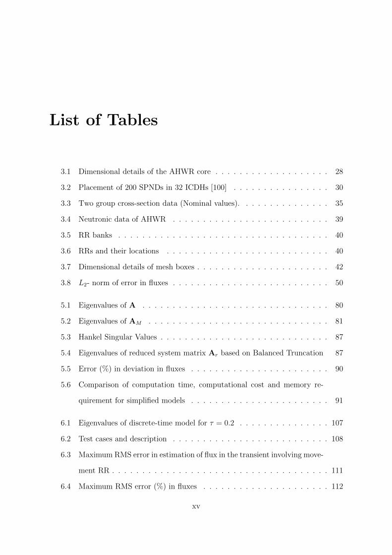
List of Tables
3.1 Dimensional details of the AHWR core . . . . . . . . . . . . . . . . . . . 28
3.2 Placement of 200 SPNDs in 32 ICDHs [100] . . . . . . . . . . . . . . . . 30
3.3 Two group cross-section data (Nominal values). . . . . . . . . . . . . . . 35
3.4 Neutronic data of AHWR . . . . . . . . . . . . . . . . . . . . . . . . . . 39
3.5 RR banks . . . . . . . . . . . . . . . . . . . . . . . . . . . . . . . . . . . 40
3.6 RRs and their locations . . . . . . . . . . . . . . . . . . . . . . . . . . . 40
3.7 Dimensional details of mesh boxes . . . . . . . . . . . . . . . . . . . . . . 42
3.8 L2- norm of error in fluxes . . . . . . . . . . . . . . . . . . . . . . . . . . 50
5.1 Eigenvalues of A . . . . . . . . . . . . . . . . . . . . . . . . . . . . . . . 80
5.2 Eigenvalues of AM . . . . . . . . . . . . . . . . . . . . . . . . . . . . . . 81
5.3 Hankel Singular Values . . . . . . . . . . . . . . . . . . . . . . . . . . . . 87
5.4 Eigenvalues of reduced system matrix Ar based on Balanced Truncation 87
5.5 Error (%) in deviation in fluxes . . . . . . . . . . . . . . . . . . . . . . . 90
5.6 Comparison of computation time, computational cost and memory re-
quirement for simplified models . . . . . . . . . . . . . . . . . . . . . . . 91
6.1 Eigenvalues of discrete-time model for τ = 0.2 . . . . . . . . . . . . . . . 107
6.2 Test cases and description . . . . . . . . . . . . . . . . . . . . . . . . . . 108
6.3 Maximum RMS error in estimation of flux in the transient involving move-
ment RR . . . . . . . . . . . . . . . . . . . . . . . . . . . . . . . . . . . . 111
6.4 Maximum RMS error (%) in fluxes . . . . . . . . . . . . . . . . . . . . . 112
xv

Rajasekhar. A: Computation of Neutron Flux Distribution in Large Nuclear Reactorsvia Reduced Order Modeling
6.5 Absolute relative average error ( %) in fluxes . . . . . . . . . . . . . . . . 117
6.6 Maximum and minimum relative error (%) in channels . . . . . . . . . . 117
6.7 Absolute relative error in quadrant and core average flux . . . . . . . . . 117
6.8 Error Statistics in case of Xenon-Induced Spatial Oscillations . . . . . . . 120
xvi
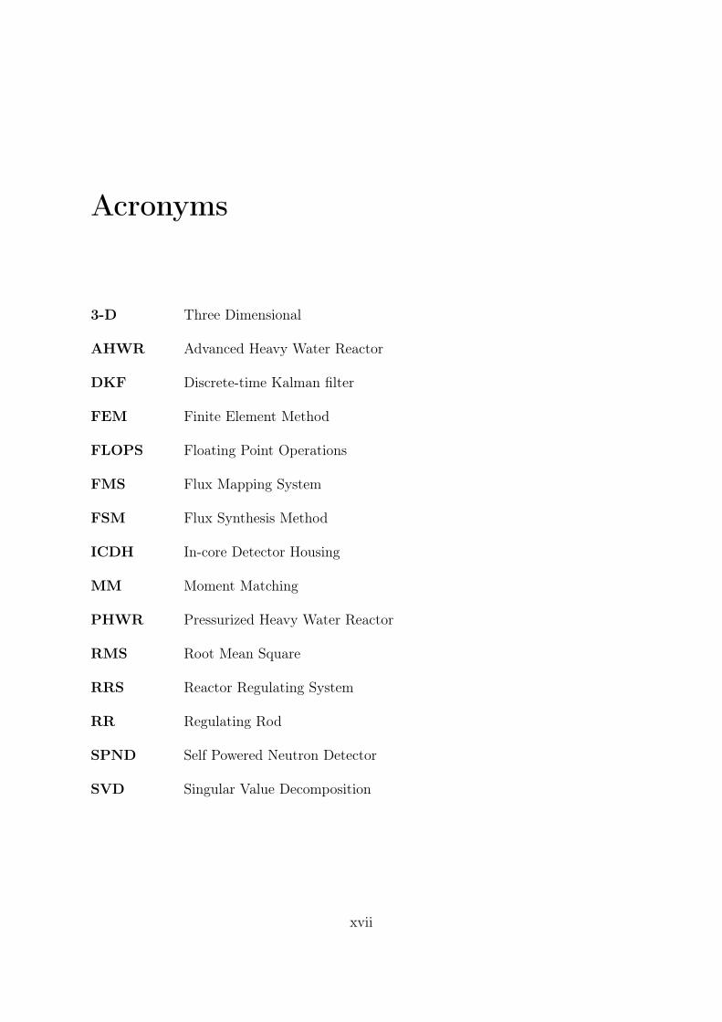
Acronyms
3-D Three Dimensional
AHWR Advanced Heavy Water Reactor
DKF Discrete-time Kalman filter
FEM Finite Element Method
FLOPS Floating Point Operations
FMS Flux Mapping System
FSM Flux Synthesis Method
ICDH In-core Detector Housing
MM Moment Matching
PHWR Pressurized Heavy Water Reactor
RMS Root Mean Square
RRS Reactor Regulating System
RR Regulating Rod
SPND Self Powered Neutron Detector
SVD Singular Value Decomposition
xvii
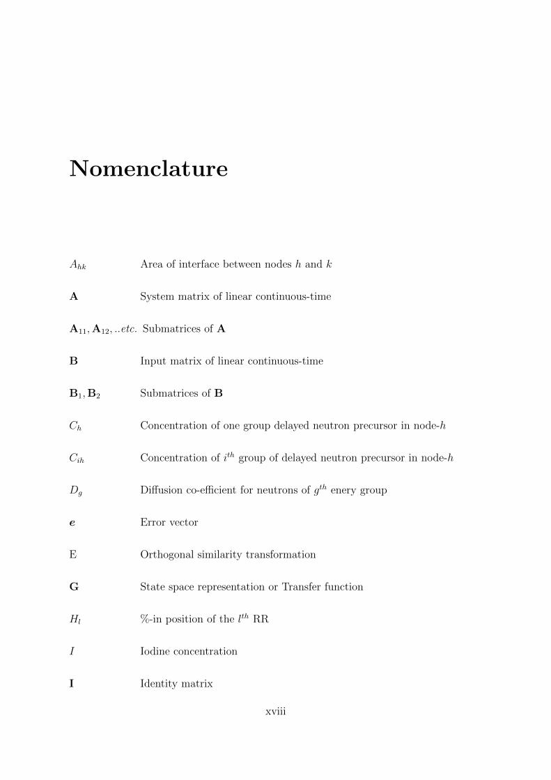
Nomenclature
Ahk Area of interface between nodes h and k
A System matrix of linear continuous-time
A11,A12, ..etc. Submatrices of A
B Input matrix of linear continuous-time
B1,B2 Submatrices of B
Ch Concentration of one group delayed neutron precursor in node-h
Cih Concentration of ith group of delayed neutron precursor in node-h
Dg Diffusion co-efficient for neutrons of gth enery group
e Error vector
E Orthogonal similarity transformation
G State space representation or Transfer function
Hl %-in position of the lth RR
I Iodine concentration
I Identity matrix
xviii

Nomenclature
Ju Neutron current density in u
Kh Multiplication factor in node-h
K Kalman gain
LO,LR Cholesky factors
m number of inputs
md Total number of delayed neutron precrsor groups
n Original system order
n1 Order of slow subsystem
n2 Order of fast subsystem
Nh Number of all neighbouring nodes to node-h
p number of outputs
P Covariance matrix of state estimate
Q Covariance matrix of process noise
r Reduced system order
Rh Ratio of fast neutron flux to the thermal neutron flux in the volume
element of node-h
R Covariance matrix of measurement noise
t Time variable
T Similarity transformation
u Input vector
xix
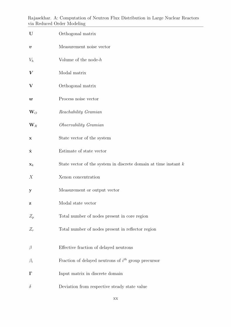
Rajasekhar. A: Computation of Neutron Flux Distribution in Large Nuclear Reactorsvia Reduced Order Modeling
U Orthogonal matrix
v Measurement noise vector
Vh Volume of the node-h
V Modal matrix
V Orthogonal matrix
w Process noise vector
WO Reachability Gramian
WR Observability Gramian
x State vector of the system
x Estimate of state vector
xk State vector of the system in discrete domain at time instant k
X Xenon concentration
y Measurement or output vector
z Modal state vector
Zp Total number of nodes present in core region
Zr Total number of nodes present in reflector region
β Effective fraction of delayed neutrons
βi Fraction of delayed neutrons of ith group precursor
Γ Input matrix in discrete domain
δ Deviation from respective steady state value
xx
Nomenclature
` Prompt neutron life-time
ε A small positive parameter
η Similarity transformation
γI Average fractional yield of Iodine
γXe Average fractional yield of Xenon
κ Scalar Weighting factor
µi Eigenvalue i
λi Decay constant of ith group of delayed neutron precursors
λI Decay constant of Iodine
λX Decay constant of Xenon
ν Mean number of fission neutrons
ω Coupling coefficient between nodes
ωhk Coupling co-efficient charecterizing leakage of neutrons from node h to k
φ One–group neutron flux
φg Neutron flux in energy group-g
Φ System matrix in discrete domain (State transition matrix)
ρh Reactivity in node-h
σ Microscopic cross-section
σ Hankel singular value
Σ Macroscopic cross-section
xxi
Rajasekhar. A: Computation of Neutron Flux Distribution in Large Nuclear Reactorsvia Reduced Order Modeling
Σ12 Scattering cross-section from group-1 to group-2
Σ21 Scattering cross-section from group-2 to group-1
Σag Absorption cross-section for energy group-g
Σfg Fission cross-section for energy group-g
τ Sampling period
4hk Center to center distance between volume elements of nodes hand k
υ Mean velocity of neutrons
υg Mean velocity of neutrons in energy group-g
Ψ Output matrix of linear continuous-time
ϑ Control signal
Operations
µ(A) Eigenvalues of A
AT Transpose of A
A−1 Inverse of A
Superscripts
0 Staeady state value
bal Balanced system
Subscripts
1 Fast group
2 Slow group
xxii
Nomenclature
a Absorption
bal Balanced system
F Fast subsystem
f Fission
G Core average flux
g Energy group
I Iodine
k Sampling instant k in discrete domain
Q Quadrant
S Slow subsystem
s Stable subsystem
us Unstable subsystem
V Volume element
X Xenon
Z Fuel channel
Other Notations
C Complex s plane
R Real space
E[.] Expected value
xxiii
Chapter 1
Introduction
Electricity is closely related to the economic development of a country. With the growth
in the number of industries utilizing fossil fuels as raw materials for production of elec-
tricity, the reserves of fossil fuels i.e., coal, oil and gas are also fast depleting. Diversified
energy resource base is essential to meet electricity requirements and to ensure long term
energy security with the limited resources of coal and oil available in any country. In
the current scenario alternative sources of energy like nuclear power, wind power and
solar power can meet the future energy demands of the nation. When compared to
other sources of energy, nuclear power has the unique capacity to release huge amount
of energy from a very small quantity of active material. The energy liberated during
this process is greater than that liberated from the combustion of the same quantity of
coal. Moreover, the possible energy reserves in the form of uranium and thorium are
many times greater than those of fossil fuels [19].
The concept of nuclear reactors has its origin in the discovery of nuclear fission in
1939. In a nuclear fission, a neutron is bombarded on a heavy nucleus such as 235U and
two or more fragments are produced. This reaction has two interesting features. One is
the significant amount of kinetic energy (about 200 MeV) of fission fragments which is
then converted into heat, and another is: a few (on the average 2 to 3) neutrons are also
produced. These facts immediately suggested the possibility of utilizing the emergent
1
Rajasekhar. A: Computation of Neutron Flux Distribution in Large Nuclear Reactorsvia Reduced Order Modeling
neutrons to cause further fissions in other heavy nuclei and thus to have a self sustained
steady fission chain reaction. Such a system, called nuclear reactor, could then act as a
steady source of energy. Since the first reactor built by Enrico Fermi in 1942, the field
has continuously evolved leading to many complex nuclear reactors of today.
Now the world wide trend is to construct nuclear reactors of large capacity which
can be operated with relatively uniform flux distribution. The Indian Nuclear power
program today comprises of existing reactors, reactors under construction, and design
of future reactors which will provide long term energy security of the country. In 2005,
a 540 Mwe Pressurized Heavy Water Reactor (PHWR) is commissioned for large-scale
electricity generation. Even a large capacity of 700 MWe PHWR and Advanced Heavy
Water Reactor (AHWR) are also under design [119]. They share several similarities
in the concept of the pressure tubes and calandria tubes, but the tubes orientation in
the AHWR is vertical and horizontal in PHWR [116]. The PHWR utilizes natural ura-
nium as fuel, whereas the AHWR utilizes enriched uranium-thorium, plutonium-thorium
mixed oxide fuels. Also, PHWR is non-boiling heavy water moderated reactor, whereas
the AHWR is boiling light water cooled, heavy water moderated natural circulation
reactor.
From the economic point of view large nuclear reactors reduce the per unit electricity
generating cost. Hence, large sized nuclear reactors are preferred to achieve economy
in power production. However, large sized reactors show neutronic decoupling [19], i.e.,
these reactors show deviation in power distribution from the nominal. Commonly used
methodology to understand the neutronic decoupling phenomena in nuclear reactors
is based on comparison of characteristic size. The characteristic size of the reactor
core is expressed in units of neutron migration length M . It is a measure of the average
distance travelled by a neutron from its appearance as a fission neutron to its absorption
as a thermal neutron. For a given reactor design, M is determined by the material
composition of the reactor core, primarily the fuel-to-moderator ratio and is essentially
independent of core size R. As the core size increases, the ratio R2/M2 increases, the
2
Chapter 1. Introduction
migration length becomes a smaller fraction of the reactor core dimension. Thus, each
neutron’s zone of influence becomes a smaller fraction of the core volume, and the various
regions of the core turn out to be loosely coupled. Any deliberate attempt to operate the
reactor with flattened radial and axial flux distributions coupled with xenon poisoning
effect leads to complex operational and control problems [114, 128]. The mechanism of
135Xe production and its removal by neutron absorption and radioactive decay are such
that oscillations of thermal flux are induced in large thermal reactors. Such oscillations
induced by 135Xe can broadly be classified into two categories - fundamental mode or
global power oscillations and higher mode or spatial oscillations. Generally speaking,
global power oscillations can be readily noticed and suppressed by control system while
spatial oscillations are not. Here, the global reactor power can remain constant so that
no change in the coolant outlet temperature is effected, the oscillations being in spatial
distribution of power inside the core.
If these oscillations are left uncontrolled, the power density and time rate of change
of power at some locations in the reactor core may exceed the respective design limits,
resulting into increased chance of fuel failure. Therefore, to maintain the total power and
power distribution within the design limits, large reactors are provided with mechanisms
for total power control and spatial power control. If due to some hypothetical reason,
the spatial control scheme is ineffective, xenon-induced oscillations might occur. These
xenon induced spatial oscillations and subsequent local overpower pose a potential threat
to the fuel integrity of the reactor. Therefore, monitoring of the axial and the radial
flux distribution in the core during the operational condition is crucial. Modern reactors
have provisions for online spatial control and monitoring of flux or power distribution
during the course of their operation. The three-dimensional (3-D) power distribution
is one of the basic operation parameters which can determine many other important
parameters such as power peaking factor, and quadrant tilt ratio etc., used to evaluate
the operating condition of the reactor and the margin of safety.
In general, the time varying neutron flux distribution in large nuclear reactors is
3

Rajasekhar. A: Computation of Neutron Flux Distribution in Large Nuclear Reactorsvia Reduced Order Modeling
computed by an online Flux Mapping System (FMS). In-core Self Powered Neutron
Detectors (SPNDs) are being increasingly used for continuous monitoring of neutron flux
in power reactors. SPNDs, which are placed at strategic locations within the core, can
help in successful implementation of both the online FMS and flux tilt control. The in-
core SPNDs used for the monitoring purpose can sense the neutron flux only over a small
volume. FMS processes the measurement signals of several in-core SPNDs with the help
of software routine called flux mapping algorithm and generates detailed 3-D core flux
profile. Apart from this, functions such as flow changes in coolant channels, reactivity
device movements and ensuring that peaking factors are within analyzed safety limits,
are also required in large reactors. These functions are performed from the information
about axial, azimuthal and radial flux distributions obtained through in-core SPNDs
based FMS. However, these functionalities of online FMS vary from reactor to reactor.
With India’s five to six times larger reserves of thorium than that of natural uranium,
thorium utilization for large scale energy production has been an important goal of the
nuclear power program. The AHWR [119] can provide efficient commercial utilization
of thorium and thereby it forms an important milestone in the nuclear power program.
The physical dimensions of the core are several times large compared to the neutron
migration length. Any operational reactivity disturbance such as online refueling, control
rod movements etc., might lead to slow xenon induced oscillations, which might cause
changes in axial and radial flux distribution from the nominal distribution. Knowledge
of any such changes during the reactor operation is crucial. To monitor the core flux
distribution, 200 SPNDs are proposed [1] to be provided in AHWR. An efficient flux
mapping algorithm in AHWR can ensure better reactor regulation and core monitoring,
as more accurate estimates of channel and zonal powers will be available to Reactor
Regulating System (RRS) and Core Monitoring System.
In nuclear reactor two basic sources of information are available for determination
of spatial flux distribution. These sources are nominal core specifications alongwith
mathematical model and measurements from in-core SPNDs, which combine through
4
Chapter 1. Introduction
flux mapping algorithms, ultimately to provide power/flux map. However, both these
sources are subjected to statistical fluctuations and the mapping accuracy may be de-
graded. Flux mapping algorithm plays a major role in mapping the 3-D flux distributions
from in-core SPNDs. And this knowledge ensures the safe operation of reactor. There-
fore, considerable effort has been expanded over the years to evolve an efficient flux
mapping algorithm.
Most of the algorithms available today employ the Flux Synthesis Method (FSM), In-
ternal Boundary Condition method and the method based on simultaneous least squares
solutions of neutron diffusion and detector response equations [80]. These methods as-
sume that the neutron flux profile in the reactor is independent of time. They fail
to account for time variation of neutron flux distribution during the reactor operation.
Also, the accuracy of mapping might be degraded considerably in presence of uncertainty
in the detector readings. Therefore, some algorithms which can take care of both time
varying phenomena and detector random errors become necessary to improve the online
computation of core power/flux distribution. In this context state estimation methods
like Kalman filter are more promising approach with the availability of the space-time
kinetics model which represents the time dependent behavior of the AHWR.
In this thesis, Discrete-time Kalman filter (DKF) formulation for flux mapping in
AHWR has been presented. It utilizes the time dependent core neutronics equations
and available detector measurements corrupted with white Gaussian noise. However,
direct implementation of the DKF algorithm to the high-order stiff estimation model of
AHWR is not feasible as the design procedure is accompanied by serious numerical ill-
conditioning caused by the simultaneous presence of slow and fast phenomena typically
present in a nuclear reactor. In particular, the set of recursive equations for computa-
tion of DKF gains, as a solution to weighted least squares problem, is ill-conditioned.
Consequently, serious numerical difficulties are expected if the DKF gain matrix is to
be computed on the basis of the full order Riccati equation. Therefore, for the AHWR
system application of model order reduction techniques, viz., Davison’s and Marshall’s
5
Rajasekhar. A: Computation of Neutron Flux Distribution in Large Nuclear Reactorsvia Reduced Order Modeling
dominant mode retention techniques; balanced truncation technique and model decom-
position into slow and fast subsystems based on singular perturbation analysis has been
explored.
Finally, to address the numerical ill-conditioning, the task of flux mapping problem
in AHWR has been formulated as a problem of optimally estimating the time dependent
neutron flux at a large number of mesh points in the core. The solution is obtained using
the well known Kalman filtering technique which works alongwith a space–time kinetics
model of the reactor. However, as stated the attempt to solve the Kalman filtering
problem in a straight forward manner is not successful due to severe numerical ill-
conditioning caused by the simultaneous presence of slow and fast phenomena, typically
present in a nuclear reactor. Hence, a grouping of state variables has been suggested
whereby the original high order model of the AHWR is decoupled into a slow subsystem
and a fast subsystem. Now according to the order of the slow and fast subsystems, the
original time update and Kalman gain equations have also been decoupled into separate
sets of equations for the slow and fast subsystems. The decoupled sets of equations
could be solved easily. The proposed method has been validated in a number of typical
transient situations. Overall accuracy in the estimation using the proposed methodology
has been found very good for mesh fluxes, channel fluxes, quadrant fluxes and the core
average flux.
Objectives of the Thesis
In large nuclear reactors such as the AHWR, the physical dimensions of the core are very
large compared to the neutron migration length. Therefore, operational perturbations
might lead to slow xenon induced oscillations, which might cause changes in axial and
radial flux distributions from the nominal distribution. Knowledge of any such changes
during the reactor operation is crucial and needs to be continuously monitored and
displayed to the operator.
6
Chapter 1. Introduction
This task is accomplished by an online Flux Mapping System, which employs a suit-
able algorithm to estimate the core flux distribution from the readings of a large number
of in-core detectors. Most of the algorithms available today employ the Flux Synthesis
method, Internal Boundary Condition method, and the method based on simultaneous
least squares solutions of neutron diffusion and detector response equations. A common
feature of these methods is the assumption that the neutron flux profile in the reactor is
independent of time. An efficient flux-mapping algorithm in AHWR can ensure better
reactor regulation and core monitoring, as more accurate estimates of channel and zonal
powers will be available to the Reactor Regulating System (RRS) and Core Monitoring
System. This thesis proposes a new method of flux mapping. Its main objectives are:
• Development of suitable mathematical model which describes the time-dependent
core neutronics behavior of the AHWR core.
• Development of a stringent nonlinear mathematical model for validation of pro-
posed flux mapping algorithm.
• To design an efficient flux mapping algorithm which accounts the time variation
of neutron flux distribution as well as random noise in detector readings.
• To investigate the applicability of different types of state observers like Kalman
filter for the estimation of 3-D neutron flux distribution.
• Evaluation and application of various model order reduction methods to handle the
numerical ill-conditioning that could arise out of existence of multiple time–scales.
• To examine the effectiveness of the proposed algorithm under different operating
transients of the reactor.
• To evaluate the efficacy of the proposed technique through simulation data.
7
Rajasekhar. A: Computation of Neutron Flux Distribution in Large Nuclear Reactorsvia Reduced Order Modeling
Contributions of the Thesis
The contributions of the thesis are as follows:
• The monitoring and control of time-varying axial and radial flux distribution in
operational large reactors is a challenging problem. Although, several researchers
addressed the flux mapping problem of the other reactors with various advanced
algorithms and methodologies, they have a common disadvantage of failing to
account the time variation and loss of accuracy in presence of random errors. The
algorithm suggested in this report is based on Kalman filtering technique which
can take care of both the stated factors.
• For validation of different techniques of flux mapping, computation results gener-
ated using a high fidelity model is a necessity. Hence, a model based on 128-nodes
in the core of the AHWR resulting into 1168th order is developed.
• Different approaches of obtaining reduced order model from the original higher
order estimation model of AHWR viz., Davison’s, Marshall’s, singular perturbation
and balanced truncation techniques have been explored to solve the numerical ill-
conditioning in control analysis and design.
• The concept of application of Kalman filtering theory has been extended to the
near optimal estimation of core flux distribution in AHWR.
• A novel technique has been suggested based on two-time-scale formulation of
Kalman filtering problem for the time-dependent neutron diffusion equation to
near-optimum estimation of the core flux profile in the AHWR.
Organization of the Thesis
The objective of this thesis is to design a flux mapping algorithm for computation of
neutron flux distribution in large nuclear reactors. For this the proposed DKF based
8
Chapter 1. Introduction
algorithm has been applied to the AHWR for different test cases and validated. The
rest of the thesis is organized as follows. Chapter 2 presents the literature survey on
existing flux mapping algorithms, model order reduction, singular perturbation methods
in control analysis and design, modeling of nuclear reactors and Kalman filtering theory.
In chapter 3, brief review of AHWR core configuration; detailed mathematical model-
ing; methods for generating steady–state neutron flux distribution and reconstruction
techniques are given. In chapter 4, theory of model order reduction and algorithmic
approach for some of the model order reduction techniques are presented. In chapter 5,
comparative study of different reduced order models of the AHWR has been presented.
In chapter 6, a two-time-scale approach for discrete-time Kalman filter has been pre-
sented to solve the numerical ill-conditioning occurred in design for computation of 3-D
flux neutron distribution. Its validation has also been illustrated with numerical and
graphical results for the AHWR. Chapter-7 draws the important conclusions from the
work and presents the future scope.
9
Chapter 2
Literature Survey
This chapter presents the literature survey of various techniques on flux mapping al-
gorithms, model order reduction techniques, singular perturbations and two-time-scale
methods for design and analysis, modeling of nuclear reactors and theory of Kalman
filter. However, this survey is not intended to be exhaustive.
2.1 Flux Mapping Algorithms
Flux mapping algorithms play fundamental role in generating the 3-D neutron flux
distribution from readings of in-core SPNDs. The knowledge of 3-D flux distribution
ensures the safe operation of reactor. In CANDU-6 reactors and in Indian 540 MWe
Pressurized Heavy Water Reactors (PHWR), 102 Vanadium detectors are used for flux
mapping, while in PWRs it is carried out by Rhodium detectors installed in about 45
fuel assemblies. Over the years, research has been carried out to evolve an efficient
flux mapping algorithm for the improvement of accuracy in flux mapping with less
computational effort. Most of the algorithms existing in the literature are based on three
principles, namely the Flux Synthesis, Internal boundary condition and simultaneous
least squares solution of neutron diffusion and detector response equations.
The most popular and traditional method for flux mapping is known as FSM [46].
10
Chapter 2. Literature Survey
It uses the available detector measurements and performs least squares fit with pre-
computed flux modes, determined based on reactivity devices configuration. Deter-
mination of flux modes requires the knowledge of core configuration and considerable
insight into the reactor operation. There are other synthesis methods such as Harmonic
Synthesis Method (HSM) [27, 95] and Harmonic Expansion Method (HEM) [133] to
improve the accuracy of flux mapping, however the accuracy of reconstruction depends
on selection of the reference case. Selection of a suitable reference case which reflects
the actual core condition results in improvement of the reconstruction accuracy. During
the core configuration changes, the reference case has to be renewed, which can be a
time consuming process.
A method based on direct online solution of neutron diffusion equations with detector
readings as the internal boundary condition is reported in [52, 59]. A method which
obtains a least squares solution of the core neutronics design equations alongwith the
in-core detector response equations is reported in [23, 47, 71]. Applicability of this least
squares method requires to solve the overdetermined system of equations resulting in
the framework of mapping algorithm. Another approach with the combination of FSM
and least squares method, known as modified flux synthesis method has been proposed
for Indian 700 MWe PHWR in [80]. This method takes longer computation time than
FSM does [47] and detector signal uncertainty can also deteriorate the performance of
flux mapping calculations. Several other approaches for flux mapping have also been
proposed. Among them a few are: Rational mapping [7], Statistical framework based
on Kalman filter and maximum likelihood estimation techniques [8], combination of
harmonic synthesis and least squares approach [136], ordinary krigging method [92], etc.
As already stated, the traditional FSM method and other synthesis methods such
as HEM, HSM, etc., have some inherent deficiencies such as pre-computation of flux
modes requiring detailed knowledge about the core configuration, considerable insight
into the reactor operation, and selection of the reference case, which needs to be renewed.
Therefore, they may not be feasible for on-line monitoring. They cannot calculate the
11

Rajasekhar. A: Computation of Neutron Flux Distribution in Large Nuclear Reactorsvia Reduced Order Modeling
time dependent neutron flux distribution during the reactor operation and the accuracy
might be degraded considerably in presence of uncertainty in the detector readings.
Hence, a new algorithm which does not require pre-computation of flux modes, and
which accounts for the time variation as well as random noise in detector measurements
would be an attractive alternative.
With this motivation we have attempted Discrete-time Kalman filter (DKF) formu-
lation for flux mapping which is quite different from the existing methods as it can take
care of both time varying phenomena and random errors in the detector readings.
2.2 Model Order Reduction
Description of large-scale systems by mathematical models involves a set of differential
or difference equations. These models can be used to simulate the system response and
predict the behavior. Sometimes, these mathematical models are also used to modify or
control the system behavior to conform with certain desired performance. In practical
control engineering applications with the increase in need for improved accuracy these
mathematical models lead to high order and complexity [2]. In many situations, high-
order, complex mathematical models accurately represent the problem at hand, but
are unsuitable for the desired application; for instance, for analysis, optimization or
for control design. Ideally, control engineer would like to develop a model with low
number of states but it should capture the system dynamics accurately over a range of
frequencies and forcing inputs.
On the other hand, well established modern control concepts which are valid for
any system order may not give fruitful control algorithms in control design. Moreover,
working with very high order, high-fidelity model involves computational complexity
and need for high storage capability. Sometimes, the presence of small time constants,
masses, etc. may give rise to an interaction among slow and fast dynamic phenomena
with attendant ill-conditioning or stiff numerical problems [65]. When analyzing and
12
Chapter 2. Literature Survey
controlling these large–scale dynamic systems, it is extremely important to look for and
to rely upon efficient simplified reduced order models which capture the main features
of the full order complex model.
In control engineering, model order reduction techniques are fundamental both to
facilitate the design of controller/observer where particular numerically heavy proce-
dures are involved (optimal control, adaptive control, H-infinity based methodologies,
filtering techniques), and to obtain low-order controllers with which to reduce hardware
requirements. In fact, from a high-order model, a low-order model must be obtained so
as to be able to design a low-order controller/observer.
An overview of model order reduction methods across the broad spectrum of ap-
proaches indicates the following scenarios. There are different approaches for model or-
der reduction of large-scale systems, the major difference being the representation/domain
of the model: either frequency or time. All the model order reduction techniques provide
high fidelity, low-order models, which are used for the modern control design applica-
tions. The model reduction techniques differ from one another by the type of model used
for approximation, whether it belongs to frequency domain or time domain. However,
this may not be crucial since it is easy to change the model representation domain.
The main reasons for obtaining low-order models are as follows [25]:
1. To have low-order models so as to simplify the understanding of a system.
2. To reduce computational efforts in simulation problems.
3. To decrease computational efforts and so make the design of the controller/observer
numerically more efficient.
4. To obtain simpler control laws and simple control structure.
The model order reduction philosophy is a common procedure in engineering prac-
tice. The concept originated way back in 1892 with the introduction of Pade approxi-
13
Rajasekhar. A: Computation of Neutron Flux Distribution in Large Nuclear Reactorsvia Reduced Order Modeling
mation but the interest of researchers was spurred only after the work of Rosenbrock on
distillation columns [97].
In the last five decades considerable attention was devoted to the problem of de-
riving reduced-order models for complex large-scale systems, without any reference to
particular system structure (MIMO-SISO). Davison [14] proposed one of the first model
reduction techniques. The principle of this method is to neglect eigenvalues of the orig-
inal system which are farthest from the origin and retains only dominant eigenvalues.
Hence, the time constants of the original system will be in the reduced order model. This
implies that the overall behavior of the reduced-order model will be very much similar to
the original model. Because, the contribution of unretained eigenvalues are important
only at the beginning of the response, whereas the eigenvalues retained are important
throughout the whole response. As pointed out subsequently by Chidambara [17], the
method does not provide for steady-state agreement between the dominant state vari-
ables of the original and reduced models. Further arguments of Chidambara and Davi-
son [15, 16] led to several variations of Davison’s original approach: Chidambara’s first
method, Chidambara’s second method and Davison’s ‘first-modified’ method. Later,
Davison [18] proposed ‘second-modified’ method. Simultaneously, Marshall [77] devel-
oped a technique which preserves the steady-state of the original system by exciting the
modes in the reduced model differently from those in the original system.
Aoki [3] proposed another systematic method to approximate the large-scale dynamic
systems by generalizing the concept of aggregation. Further, Siret et al. [120] proposed
an algorithm for obtaining the best possible approximate model by minimizing the error
criterion which results in optimal aggregation matrix as the solution of linear matrix
equation. Later, Fossard [26] proposed a modification to Davison’s original method
which ensures both initial and final (steady-state) agreement between the original and
reduced models. Several additional techniques have been developed later and the review
paper of Genesio and Milanese [35] indicates all the techniques. However, they represent
14
Chapter 2. Literature Survey
minor extensions to one or another of the procedures mentioned above.
It is of central concern to determine the number and choice of modes to be retained in
the reduced order model. However, aforesaid methods did not provide any information
on selection of eigenvalues to be retained. Therefore, attempts in this direction have been
made to select the size of the reduced order model using reduction techniques: Davison,
Marshall, and Chidambara where satisfactory dynamic and steady-state responses are
desired. Mahapatra [74, 75], Iwai and Kubo [51], Elrazaz and Sinha [20], Enright and
Kamel [22], Litz [73], Gopal et al. [39] proposed various modal techniques. These
methods are optimal in the sense that the integral of the square of the errors between
the dominant state variables in the original and approximate models is minimized.
For the state-space models, another model reduction scheme based on the assess-
ment of degree of reachability and observability, which is well grounded in theory and
most commonly used is the so-called balanced truncation first introduced by Mullis and
Roberts [82] and later extended to systems and control literature by Moore [81]. In or-
der to obtain the original system in balanced form [94], its basis should be transformed
into another basis where the states which are difficult to reach are difficult to observe.
It can be achieved by simultaneously diagonalizing the reachability and the observabil-
ity Gramians [70], which are the solution to reachability and observability Lyapunov
equations. The positive decreasing diagonal entries in the diagonal reachability and ob-
servability Gramians in the new basis are called Hankel singular values of the system.
The reduced order model is obtained simply by truncation of the states corresponding
to the smallest singular values. The number of states that can be truncated depends
on how accurate the approximate model is needed. There are some other techniques
to obtain the balanced truncation viz., optimal Hankel norm approximation [38], Schur
method [98], balanced square root method [132] similar to [81], however, they differ in
the algorithms to obtain the balancing transformation.
15
Rajasekhar. A: Computation of Neutron Flux Distribution in Large Nuclear Reactorsvia Reduced Order Modeling
The aforesaid methods can be efficiently applied when the system is asymptotically
stable and minimal, however, for the systems where the stabilization is the major concern
their straightforward application is not possible. Balanced truncation for stable nonmin-
imal systems has been attempted in [131]. Balanced truncation for unstable systems has
also been attempted in [5, 57, 99]. Usually unstable poles cannot be neglected, therefore
model reduction in this situation can be treated by first separating the stable and un-
stable parts of the model and then reducing the order of the stable part using balanced
truncation methods. Pertinent literature survey on balanced truncation methods and
obtaining balanced transformation procedure can be found in [2, 5, 42, 93]. Balanced
truncation is probably the most popular projection and Singular Value Decomposition
(SVD) based method. Moment Matching (MM), known as Krylov Methods, such as
Lanczos method, Arnoldi method, etc., combination of SVD and MM, known as SVD-
Krylov Methods are also available for model order reduction. A good review of these
methods has been presented in [2]. Enns [21] has extended the balanced truncation
scheme to the frequency weighted case by modifying the controllability/observability
Gramians to reflect the presence of the input/output weights. A review of frequency
weighted balanced model reduction techniques has been presented in [36].
In frequency domain approach also, several methods have been reported for model
order reduction. Among them, the important methods are Pade approximations [106],
Routh approximations [49], moment matching techniques, Pade and modal analysis
[107], continued fraction [10], and combination of Routh stability criterion and Pade
approximation [108]. Other contributions for model order reduction of discrete time
models can be found such as continued fraction/Pade approach [45, 105], LMI based
approaches [40], multi-point continued fraction and Pade approximations [72], stability
preserving methods [11, 109], optimal approaches [45]. A good review on the available
techniques can also be found in [2, 25, 89, 121, 128].
16

Chapter 2. Literature Survey
2.3 Singular Perturbation Theory and Time–Scale
Methods
Singular perturbation theory/techniques have been a traditional tool of fluid dynamics
the modeling, analysis and design of control systems [60]. Their use has spread to
other areas of mathematical physics and engineering, where the same terminology of
“boundary layers” and “inner” and “outer” matched asymptotic expansions continued
to be used. In control systems, boundary layers are a characteristic of system’s two-
time scale behavior. They appear as initial and terminal “fast transients” of state
trajectories and represent the “high-frequency” parts of the system response. High-
frequency and low-frequency models of dynamical systems such as electrical circuits
etc., which have had a long history of their own, are naturally incorporated in the time-
scale methodology. Singular perturbation theory also includes diverse problem-specific
applications. For robotic manipulators, the slow manifold approach has been employed
to separately design the slow (rigid system) dynamics and the fast (flexible) transients.
Electric machines, power systems and nuclear reactor systems have been the areas of
major applications of multi-time scale methods for aggregate (reduced order) modeling
and transient stability studies. Singular perturbations are continue to be among the
frequently used tools in nuclear reactor kinetics and also in flight dynamics etc.
The versatility of singular perturbation methods is due to their use of time–scale
properties, common to both linear and nonlinear systems. However, this survey reviews
the most special class of linear dynamical systems which are known as singularly per-
turbed systems. These are characterized by the presence of slow and fast variables, in
the dynamics of many real–time systems such as power systems, nuclear reactor etc.
Mathematically, the slow and fast phenomena are characterized by small and large time
constants, or by system eigenvalues that are clustered into two disjoint sets. The slow
system variables corresponds to the set of eigenvalues closer to the imaginary axis, and
the fast system variables are represented by the set of eigenvalues that are far from the
17
Rajasekhar. A: Computation of Neutron Flux Distribution in Large Nuclear Reactorsvia Reduced Order Modeling
imaginary axis.
Singular perturbations and time–scale techniques were introduced to control engi-
neering in the late 1960s and have since become common tools for modeling, analysis
and design of control systems for a variety of applications including state feedback, out-
put feedback, Kalman filter and observer design. These techniques were first applied
to optimal control and regulator design by Kokotovic et.al. [66]. Modeling of singu-
larly perturbed continuous and discrete–time systems is presented in [125]. Singularly
perturbed systems and time-scale methods have been studied extensively in last five
decades [60, 62, 64]. Survey of singular perturbations and time scale methods in control
theory and applications prior to 2001 has been presented in [65, 87, 102]. A more recent
review of singular perturbations and time-scale methods in control theory and applica-
tions such as optimal control, robust control, fuzzy control, network control, H2/H∞
control, stability analysis, numerical algorithms and other control problems during the
period 2002-2014 has been presented in [135].
Singular perturbation methods are also useful for model order reduction. The or-
der reduction procedure and its validation for both linear and nonlinear systems can
be found in [65]. The approach makes use of the standard singularly perturbed form
representation of dynamic systems in which the derivatives of some state variables are
multiplied with a small positive scalar, ε. The model reduction is achieved by setting
ε = 0 and substituting the solution of states whose derivatives were multiplied with ε,
in terms of the other state variables. Essentially the singular perturbation approach to
order reduction can be related to the “dominant mode” technique [14, 15, 16, 17, 18, 77]
which neglect the “high frequency” parts and retain “low frequency” parts of models.
In application, models of physical systems are put in the standard singularly perturbed
form by expressing small time constants, small masses, large gains, etc., in terms of ε.
In power system models, ε can represent machine reactances or transients in voltage
regulators; in industrial control systems it may represent time constants of drives and
actuators; and in nuclear reactor models it is due to prompt neutrons [128]. Singular
18
Chapter 2. Literature Survey
perturbations are extensively used in aircraft and rocket flight models and in chemi-
cal reaction diffusion theory. Many order reduction techniques can be interpreted as
singular perturbations [48, 104]. An alternate approach for the study of singularly per-
turbed linear systems with multi parameters and multi–time scales is given by Ladde
et.al. [68, 69]. Detailed exposition of applications of singular perturbation analysis and
time–scale methods in various fields has been given in [87].
Explicit decoupling transformations play very important role in the singularly per-
turbed systems containing small parameters. Under certain, usually very mild condi-
tions, these transformations allow the linear system decomposition into independent
two reduced-order subsystems viz. slow and fast. The decoupling transformation for
linear singularly perturbed continuous–time varying systems is introduced in [9]. Re-
cursive methods for linear singularly perturbed continuous–time invariant systems are
presented in [12, 32, 63] and for discrete–time systems in [76] , in the spirit of parallel
and distributed computations and parallel processing of information in terms of reduced
order, independent, approximate slow and fast filters. These recursive techniques are
also applicable to almost all areas of optimal control theory, in context of continuous
and discrete–time, deterministic and stochastic singularly perturbed systems.
The procedure used for the time–scale decomposition of the algebraic Riccati equa-
tion into pure-slow and pure-fast algebraic Riccati equations facilitates a new insight
into optimal filtering and control problems of linear systems [29]. The filtering problem
for linear singularly perturbed continuous-time systems has been well documented in
control theory literature [28, 32, 43, 44, 58, 62]. In [43, 44], a sub optimal slow and fast
Kalman filters were constructed for the estimates of the state trajectories. In [32, 58],
both the slow and fast Kalman filters are obtained using Taylor series [58] or fixed-point
iterations [28] to calculate the corresponding filter parameters. The singularly perturbed
discrete–time Kalman filter has been studied in [31, 55, 96]. The approaches presented
in [55, 96] are based on the power series expansion. The recursive approach presented in
[31], based on fixed-point iterations to the discrete-time filtering of singularly perturbed
19

Rajasekhar. A: Computation of Neutron Flux Distribution in Large Nuclear Reactorsvia Reduced Order Modeling
systems achieves high accuracy for estimation. However, slow and fast filters are driven
by the innovation process so that the additional communication channels have to be used
in order to construct the innovation process. The results presented in [31] have been
improved in [30] by deriving the pure-slow and pure-fast, reduced order, independent
Kalman filter driven by system measurements. The method presented in [30] is based on
exact decomposition of the global singularly perturbed algebraic filter Riccati equation
into the pure-slow and pure-fast local algebraic filter Riccati equations.
It is well known that physical systems like nuclear reactor exhibit simultaneous dy-
namics of different speeds. Model decomposition based on singular perturbation and
time–scale methods for controller design for reactors have also been applied for PHWR
in [129, 130] and for AHWR in [83, 84, 85, 111, 112]. Singular perturbation methods in
Kalman filter design are reported in [55, 67, 90, 96, 110].
2.4 Modeling of Nuclear Reactors
Large sized nuclear reactors are preferred to achieve economic power production. How-
ever, large sized reactors may show spatial instability [114, 128], i.e., these reactors
experience deviation in power distribution under certain transients. Their characteris-
tics also change with fuel burn-up and operating power level. Therefore, analysis and
control of neutron flux variation with respect to time within the reactor core is required.
Usually, the variations are associated with long or short term changes induced by nat-
ural perturbations or imposed transients. For the analysis and control of the reactor
under these transients and for ensuring safety and economy of operation, mathematical
models need to be developed.
Nuclear reactors of small and medium size are generally described by the point-
kinetics model, which characterizes every point in the reactor by an amplitude factor
and a time dependent spatial shape function [37]. A major limitation of this model is that
it cannot provide any information about the spatial flux/power distribution inside the
20
Chapter 2. Literature Survey
reactor core, and it is not valid in case of large reactors because the flux shape undergoes
appreciable variation with time. Therefore, explicit consideration of the variation of the
flux shape becomes necessary.
The central problem in analysis of large nuclear reactors is the determination of the
spatial flux and power distribution in the reactor core under steady-state as well as
transient operating conditions. There is, however, a considerable variation in the degree
of accuracy and spatial details of the power distribution required in different facets of
reactor analysis and design. Basically, the behavior of neutrons in a nuclear reactor is
adequately described by the time-dependent Boltzmann transport equation [19]. How-
ever, numerical solutions of the coupled time-dependent transport and delayed neutron
precursor’s equations for reactor kinetics problems of practical interest are prohibitively
difficult. So, approximate methods using the time-dependent group diffusion equations
are employed. These methods can broadly be classified as space-time factorization meth-
ods, modal methods and direct methods [124].
Space–time factorization methods involve a factorization of the space and time de-
pendent flux into a product of two parts. One part, called amplitude function, depends
only on the time variable whereas the second part, called shape function, includes all of
the space and energy dependence and is only weakly dependent on time [50, 91].
Modal methods, on the other hand, utilize an expansion of the flux in terms of
precomputed time-independent spatial distributions through a set of time-dependent
group expansion coefficients [123]. Another class of spatial methods called synthesis
methods, which are almost equivalent to modal methods, are also prevalent. These
methods use expansion functions that are static solutions of the diffusion equation for
some specified set of initial conditions. Synthesis methods can often yield acceptable
accuracy with a smaller number of expansion functions. However, selection of expansion
functions for synthesis methods requires considerable experience.
Direct space–time methods solve the time-dependent group diffusion equations by
partitioning the reactor spatial domain into a finite number of elemental volumes,
21
Rajasekhar. A: Computation of Neutron Flux Distribution in Large Nuclear Reactorsvia Reduced Order Modeling
thereby obtaining spatially discretized forms of the coupled diffusion and delayed neutron
precursors equations. Direct methods are further classified as finite difference methods,
coarse-mesh methods and nodal methods [124]. In each of these methods, the reactor
spatial domain is discretized by superimposing a computational mesh and the material
properties are treated as uniform within each mesh box. Another method is the Finite
Element Method (FEM) in which the group flux is approximated as the sum of multi-
dimensional polynomials that are identically zero everywhere outside some elemental
volume, or as higher order polynomials thereof [41].
Application of FEM and finite difference methods requires a relatively fine mesh
to ensure accuracy, which makes them computationally intensive. On the contrary,
coarse-mesh methods assume that the reactor may be adequately described by a model
consisting of homogeneous regions that are relatively large. Determination of the multi-
dimensional flux distribution within a mesh box is an integral part of the solution process.
Like coarse-mesh methods, nodal methods also consider the division of the reactor
core into relatively large, non-overlapping nodes. However, direct results of the solution
process are often the node averaged fluxes. These methods generally demand additional
relationships between the face averaged currents and the node averaged fluxes, often
denoted as coupling parameters. The coupling parameters can be obtained from accurate
reference calculations to relate the node interface averaged currents to the node averaged
fluxes [56]. A nodal model with finite difference approximation of multi-group diffusion
equation has been developed for PHWR [128].
AHWR is a large nuclear reactor which requires a space–time kinetics model for
accurate representation of the time dependent neutron flux behavior. In [116], a nodal
model for AHWR, which exhibits all the essential control related properties and yields
accurate response characteristics is developed. The same model is reformulated in terms
of neutron flux equations in [101]. This model is more suitable for flux distribution
studies in AHWR owing to its simplicity and structure, thus facilitating selection of
state variables for the system in a straightforward manner. Nodal methods have been
22
Chapter 2. Literature Survey
used extensively for the analysis and simulation of Light Water Reactors and control
system design of PHWR [126, 128]. Nodal methods have also been used for designing
advanced controllers for AHWR [85, 111, 112, 115].
2.5 State Estimation and Theory of Kalman Filter-
ing
Many real–time processes require to measure a large number of system state variables
so as to own a sufficient quantity and quality of information on the system state and
to ensure the required level of performance. However, the measurement of such a large
number of physical states may not desirable as it indirectly decreases the reliability
of the system and measurement of some physical states may not be possible directly.
Sometimes, number of measurements are also limited to keep the failure rate minimum
and to increase the reliability of the system. In this context, state estimation theory has
played a major role in many applications, including without being exhaustive, trajectory
estimation, state prediction for control or diagnosis, data merging and so on.
The state of a dynamical system is a set of variables that provide a complete rep-
resentation of the internal condition or status of the system at a given instant of time
[117]. When the state is known, the evolution of the system can be predicted if the
excitations are known. Another way to say the same is that the state consists of system
variables that prescribe the initial condition. When a model of the physical system is
available, its dynamic behavior can be estimated for a given input by solving the dynam-
ical equations. However, if the physical system is subjected to unknown disturbances
and is partially instrumented, the response at the unmeasured degrees of freedom is
obtained using state estimation. It is applicable to virtually all areas of engineering and
science. Any discipline that is concerned with the mathematical modeling of its systems
is a likely (perhaps inevitable) candidate for state estimation. This includes electri-
23

Rajasekhar. A: Computation of Neutron Flux Distribution in Large Nuclear Reactorsvia Reduced Order Modeling
cal engineering, mechanical engineering, chemical engineering, aerospace engineering,
robotics, economics, ecology, biology, and many others. The possible applications of
state estimation theory are limited only by the engineer’s imagination, which is why
state estimation has become such a widely researched and applied discipline in the past
few decades.
Estimation is the process of extracting information from all the data: data which
can be used to infer the desired information and may contain errors. Modern estimation
methods use known relationships to compute desired information from the measure-
ments, taking account of measurement errors, the effects of disturbances and control
actions on the system, and prior knowledge of the information. Diverse measurements
can be blended to form “best” estimates, and information which is unavailable for mea-
surement can be approximated in an optimal fashion [34].
The theory of state estimation originated with least squares method essentially es-
tablished by the early 1800s with the work of Gauss [33]. The mathematical framework
of modern theory of state estimation originated with the work of Wiener in the late
1940s, [134]. The field began to mature in the 1960’s and 1970’s after a milestone con-
tribution was offered by R. E. Kalman in 1960 [53], which is very well-known as the
Kalman filter. The Kalman filter is a recursive data processing algorithm, which gives
the optimal state estimates of the systems that are subjected to stationary stochastic
disturbances with known covariances.
Kalman filtering is an optimal state estimation process applied to a dynamical system
that involves random perturbations. More precisely, the Kalman filter gives a linear,
unbiased, and minimum error variance recursive algorithm to optimally estimate the
unknown state of a dynamic system from noisy data taken at discrete-time intervals. It
has been widely used in many industrial applications such as tracking systems, satellite
navigation, and ballistic missile trajectory estimation etc. With the recent advances in
high speed computing technology, DKF has become more useful for real-time complex
applications. Some applications of Kalman filter to nuclear reactor systems can be found
24
Chapter 2. Literature Survey
in [6, 79].
The derivations for the Kalman filter and required mathematical background have
been presented many times in the literature [34, 78, 117, 122]. Instead of reiterating
these derivations, the basic algorithm has been presented in a later chapter.
2.5.1 Numerical ill-conditioning in Kalman Filters
Kalman filter design for high dimensional systems having interaction phenomena of slow
and fast dynamics tends to suffer from numerical ill-conditioning [127]. Least squares
problem generally gives rise to particularly ill-conditioned matrix inversion problems.
Considering that Kalman filter is simply a recursive solution to a certain weighted least
squares problem, it is not surprising that Kalman filter tends to be ill-conditioned. An
awareness of ill-conditioning of Kalman filter was achieved after the nontrivial applica-
tions of [24] and [103]. Fine exposition of this computational difficulty has been given
in [54] and detailed discussion has been given in [13].
25
Chapter 3
Mathematical modeling of
Advanced Heavy Water Reactor
3.1 Brief description of the AHWR
In India, the AHWR is being designed to utilize the large amounts of thorium reserves
with the objective of commercial power generation to provide the long term energy
security of the nation [119]. Thorium in its natural state does not contain any fissile
isotope as uranium does, therefore the AHWR utilizes enriched mixed oxide fuels such
as uranium-thorium and plutonium-thorium. The current design of the AHWR is of 920
MW (thermal), vertical, pressure tube type, heavy water moderated and boiling light
water cooled thermal reactor. Its core is surrounded by a low pressure reactor–vessel
called calandria containing heavy water which acts as moderator and reflector. It relies
on removal of the heat generated in the fuel by natural circulation of the coolant.
The AHWR is much like the PHWR, in that they share similarities in the concept
of the pressure tubes and calandria tubes, but the tube’s orientation in the AHWR is
vertical, unlike that of the PHWR. The reactor design incorporates advanced technolo-
gies, together with several proven positive features of Indian PHWRs. These features
include pressure tube type design, low pressure moderator, on-power refueling, diverse
26
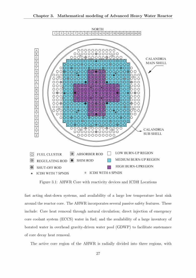
Chapter 3. Mathematical modeling of Advanced Heavy Water Reactor
Figure 3.1: AHWR Core with reactivity devices and ICDH Locations
fast acting shut-down systems, and availability of a large low temperature heat sink
around the reactor core. The AHWR incorporates several passive safety features. These
include: Core heat removal through natural circulation; direct injection of emergency
core coolant system (ECCS) water in fuel; and the availability of a large inventory of
borated water in overhead gravity-driven water pool (GDWP) to facilitate sustenance
of core decay heat removal.
The active core region of the AHWR is radially divided into three regions, with
27
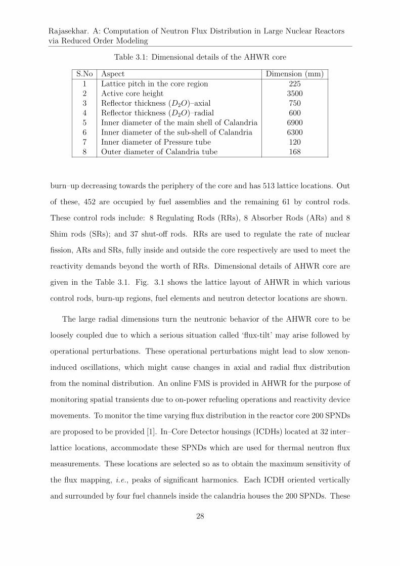
Rajasekhar. A: Computation of Neutron Flux Distribution in Large Nuclear Reactorsvia Reduced Order Modeling
Table 3.1: Dimensional details of the AHWR core
S.No Aspect Dimension (mm)1 Lattice pitch in the core region 2252 Active core height 35003 Reflector thickness (D2O)–axial 7504 Reflector thickness (D2O)–radial 6005 Inner diameter of the main shell of Calandria 69006 Inner diameter of the sub-shell of Calandria 63007 Inner diameter of Pressure tube 1208 Outer diameter of Calandria tube 168
burn–up decreasing towards the periphery of the core and has 513 lattice locations. Out
of these, 452 are occupied by fuel assemblies and the remaining 61 by control rods.
These control rods include: 8 Regulating Rods (RRs), 8 Absorber Rods (ARs) and 8
Shim rods (SRs); and 37 shut-off rods. RRs are used to regulate the rate of nuclear
fission, ARs and SRs, fully inside and outside the core respectively are used to meet the
reactivity demands beyond the worth of RRs. Dimensional details of AHWR core are
given in the Table 3.1. Fig. 3.1 shows the lattice layout of AHWR in which various
control rods, burn-up regions, fuel elements and neutron detector locations are shown.
The large radial dimensions turn the neutronic behavior of the AHWR core to be
loosely coupled due to which a serious situation called ‘flux-tilt’ may arise followed by
operational perturbations. These operational perturbations might lead to slow xenon-
induced oscillations, which might cause changes in axial and radial flux distribution
from the nominal distribution. An online FMS is provided in AHWR for the purpose of
monitoring spatial transients due to on-power refueling operations and reactivity device
movements. To monitor the time varying flux distribution in the reactor core 200 SPNDs
are proposed to be provided [1]. In–Core Detector housings (ICDHs) located at 32 inter–
lattice locations, accommodate these SPNDs which are used for thermal neutron flux
measurements. These locations are selected so as to obtain the maximum sensitivity of
the flux mapping, i.e., peaks of significant harmonics. Each ICDH oriented vertically
and surrounded by four fuel channels inside the calandria houses the 200 SPNDs. These
28
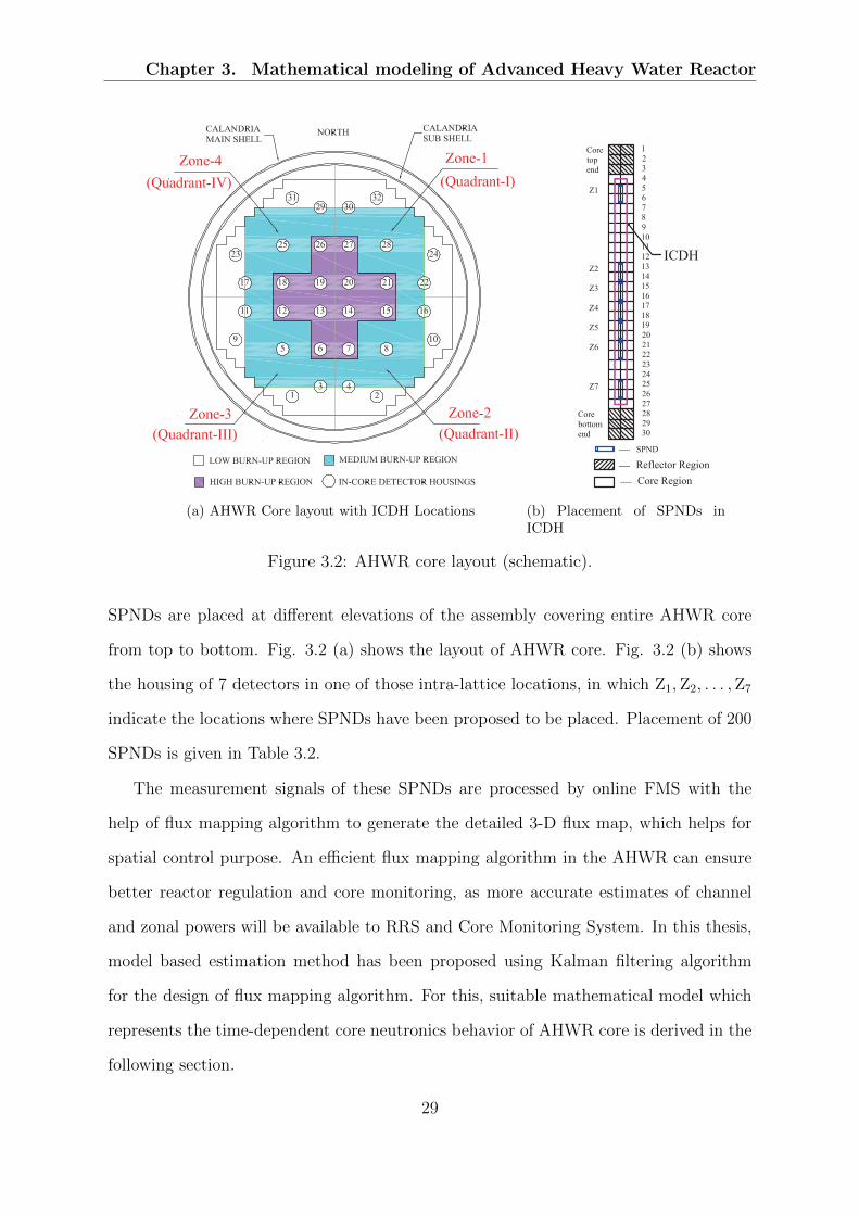
Chapter 3. Mathematical modeling of Advanced Heavy Water Reactor
(a) AHWR Core layout with ICDH Locations
ICDH
Z1
Z2
Z3
Z4
Z5
Z6
Z7
1
23
4
56
78
9
1011
12
1314
15
1617
1819
20
2122
23
2425
26
2728
2930
----- Reflector Region
Core
bottom
end
----- SPND
----- Core Region
Core
top
end
(b) Placement of SPNDs inICDH
Figure 3.2: AHWR core layout (schematic).
SPNDs are placed at different elevations of the assembly covering entire AHWR core
from top to bottom. Fig. 3.2 (a) shows the layout of AHWR core. Fig. 3.2 (b) shows
the housing of 7 detectors in one of those intra-lattice locations, in which Z1,Z2, . . . ,Z7
indicate the locations where SPNDs have been proposed to be placed. Placement of 200
SPNDs is given in Table 3.2.
The measurement signals of these SPNDs are processed by online FMS with the
help of flux mapping algorithm to generate the detailed 3-D flux map, which helps for
spatial control purpose. An efficient flux mapping algorithm in the AHWR can ensure
better reactor regulation and core monitoring, as more accurate estimates of channel
and zonal powers will be available to RRS and Core Monitoring System. In this thesis,
model based estimation method has been proposed using Kalman filtering algorithm
for the design of flux mapping algorithm. For this, suitable mathematical model which
represents the time-dependent core neutronics behavior of AHWR core is derived in the
following section.
29

Rajasekhar. A: Computation of Neutron Flux Distribution in Large Nuclear Reactorsvia Reduced Order Modeling
Table 3.2: Placement of 200 SPNDs in 32 ICDHs [100]
ICDH Layer No. No. ofNo. Z1 Z2 Z3 Z4 Z5 Z6 Z7 SPNDs
1 D1 - D41 D73 D105 D137 D169 62 D2 - D42 D74 D106 D138 D170 63 D3 - D43 D75 D107 D139 D171 64 D4 - D44 D76 D108 D140 D172 65 D5 D33 D45 D77 D109 D141 D173 76 D6 - D46 D78 D110 D142 D174 67 D7 - D47 D79 D111 D143 D175 68 D8 D34 D48 D80 D112 D144 D176 79 D9 - D49 D81 D113 D145 D177 610 D10 - D50 D82 D114 D146 D178 611 D11 - D51 D83 D115 D147 D179 612 D12 - D52 D84 D116 D148 D180 613 D13 D35 D53 D85 D117 D149 D181 714 D14 D36 D54 D86 D118 D150 D182 715 D15 - D55 D87 D119 D151 D183 616 D16 - D56 D88 D120 D152 D184 617 D17 - D57 D89 D121 D153 D185 618 D18 - D58 D90 D122 D154 D186 619 D19 D37 D59 D91 D123 D155 D187 720 D20 D38 D60 D92 D124 D156 D188 721 D21 - D61 D93 D125 D157 D189 622 D22 - D62 D94 D126 D158 D190 623 D23 - D63 D95 D127 D159 D191 624 D24 - D64 D96 D128 D160 D192 625 D25 D39 D64 D97 D129 D161 D193 726 D26 - D66 D98 D130 D162 D194 627 D27 - D67 D99 D131 D163 D195 628 D28 D40 D68 D100 D132 D164 D196 729 D29 - D69 D101 D133 D165 D197 630 D30 - D70 D102 D134 D166 D198 631 D31 - D71 D103 D135 D167 D199 632 D32 - D72 D104 D136 D168 D200 6
30
Chapter 3. Mathematical modeling of Advanced Heavy Water Reactor
3.2 Space–time kinetics modeling of AHWR
The central problem in the reactor analysis is the determination of the spatial flux and
power distribution in the reactor core under steady–state as well as transient operating
conditions as these minute details have significant importance in reactor control. The
first and foremost difficulty in operation and control of large thermal nuclear reactors
such as the AHWR is the development of suitable mathematical model for analysis. As
already stated, reactors with small core size are adequately represented by the well-
known point kinetics model. In large reactor core, the flux shape undergoes nonuniform
variations which the point kinetics model fails to capture.
The behavior of neutrons in the reactor is adequately described by the time–dependent
Boltzman transport equation. However, the numerical solution of the coupled time–
dependent transport and delayed neutron precursor’s equations for reactor kinetics stud-
ies may not be feasible. In recent times, multi-point kinetics or nodal models have been
extensively used for the analysis and simulation of Light Water Reactors and control
design of large thermal reactors such as the PHWR and AHWR. In the following sub-
sections, a reasonably accurate space–time kinetics model which describes the time–
dependent neutronics behavior of the AHWR core has been derived. It can be used
for the purpose of estimation of neutron flux using DKF based flux mapping algorithm.
This mathematical model is more suitable for flux distribution studies owing to its sim-
plicity and the structure, thus facilitating selection of state variables for the system in
a straightforward manner. It assumes that the reactor spatial domain is divided into
relatively large number of rectangular parallelopiped shaped regions called nodes which
are coupled through neutron diffusion. Neutron flux and other parameters in each node
are represented by homogenized values integrated over its volume and the degree of
coupling among these nodes is given by coupling coefficients.
31
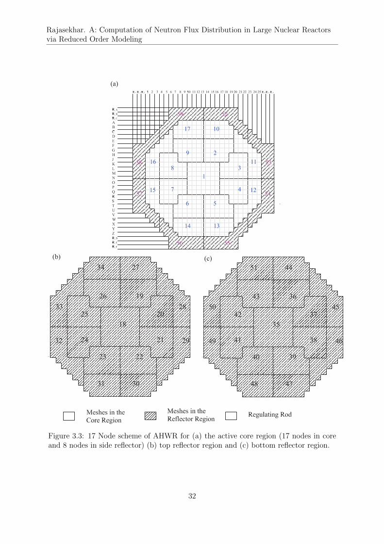
Rajasekhar. A: Computation of Neutron Flux Distribution in Large Nuclear Reactorsvia Reduced Order Modeling
Figure 3.3: 17 Node scheme of AHWR for (a) the active core region (17 nodes in coreand 8 nodes in side reflector) (b) top reflector region and (c) bottom reflector region.
32
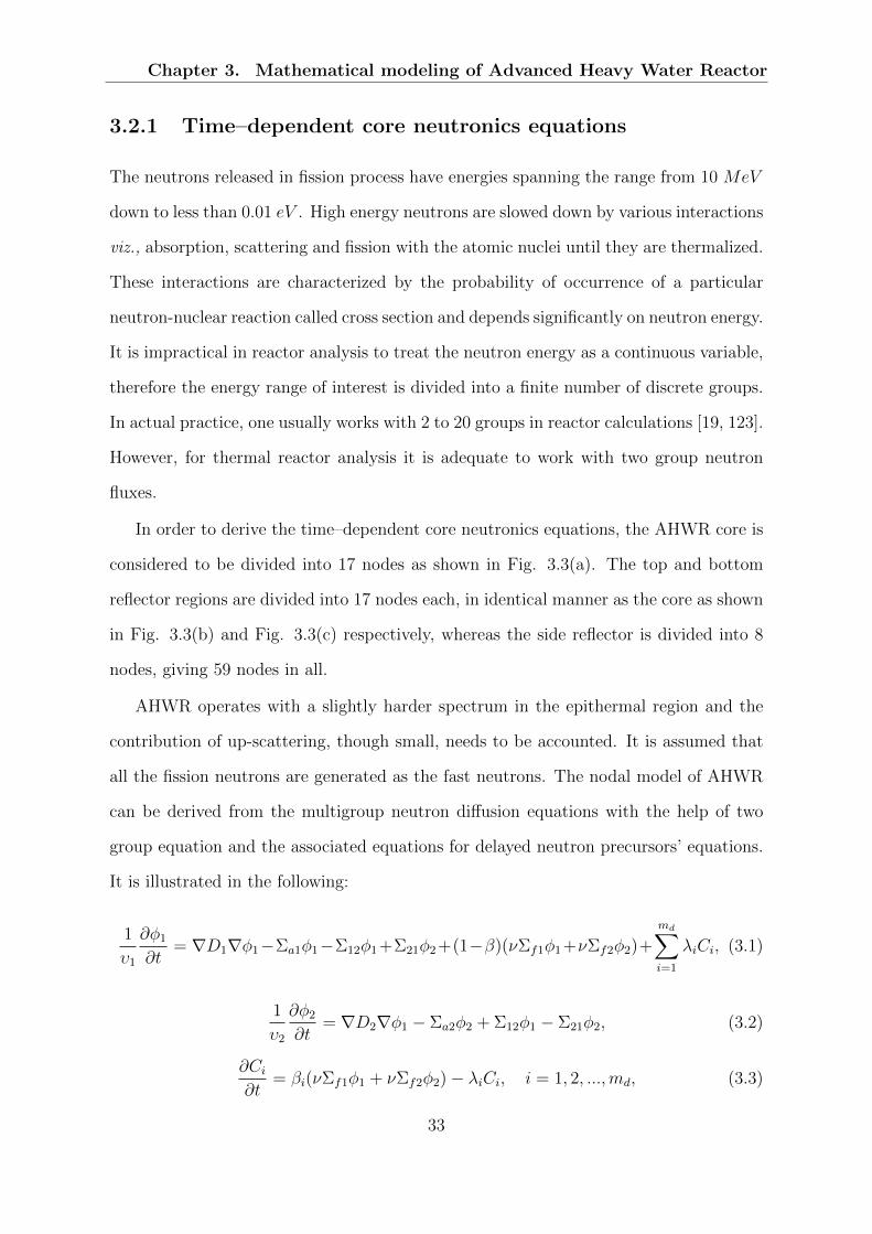
Chapter 3. Mathematical modeling of Advanced Heavy Water Reactor
3.2.1 Time–dependent core neutronics equations
The neutrons released in fission process have energies spanning the range from 10 MeV
down to less than 0.01 eV . High energy neutrons are slowed down by various interactions
viz., absorption, scattering and fission with the atomic nuclei until they are thermalized.
These interactions are characterized by the probability of occurrence of a particular
neutron-nuclear reaction called cross section and depends significantly on neutron energy.
It is impractical in reactor analysis to treat the neutron energy as a continuous variable,
therefore the energy range of interest is divided into a finite number of discrete groups.
In actual practice, one usually works with 2 to 20 groups in reactor calculations [19, 123].
However, for thermal reactor analysis it is adequate to work with two group neutron
fluxes.
In order to derive the time–dependent core neutronics equations, the AHWR core is
considered to be divided into 17 nodes as shown in Fig. 3.3(a). The top and bottom
reflector regions are divided into 17 nodes each, in identical manner as the core as shown
in Fig. 3.3(b) and Fig. 3.3(c) respectively, whereas the side reflector is divided into 8
nodes, giving 59 nodes in all.
AHWR operates with a slightly harder spectrum in the epithermal region and the
contribution of up-scattering, though small, needs to be accounted. It is assumed that
all the fission neutrons are generated as the fast neutrons. The nodal model of AHWR
can be derived from the multigroup neutron diffusion equations with the help of two
group equation and the associated equations for delayed neutron precursors’ equations.
It is illustrated in the following:
1
υ1
∂φ1
∂t= ∇D1∇φ1−Σa1φ1−Σ12φ1+Σ21φ2+(1−β)(νΣf1φ1+νΣf2φ2)+
md∑i=1
λiCi, (3.1)
1
υ2
∂φ2
∂t= ∇D2∇φ1 − Σa2φ2 + Σ12φ1 − Σ21φ2, (3.2)
∂Ci∂t
= βi(νΣf1φ1 + νΣf2φ2)− λiCi, i = 1, 2, ...,md, (3.3)
33
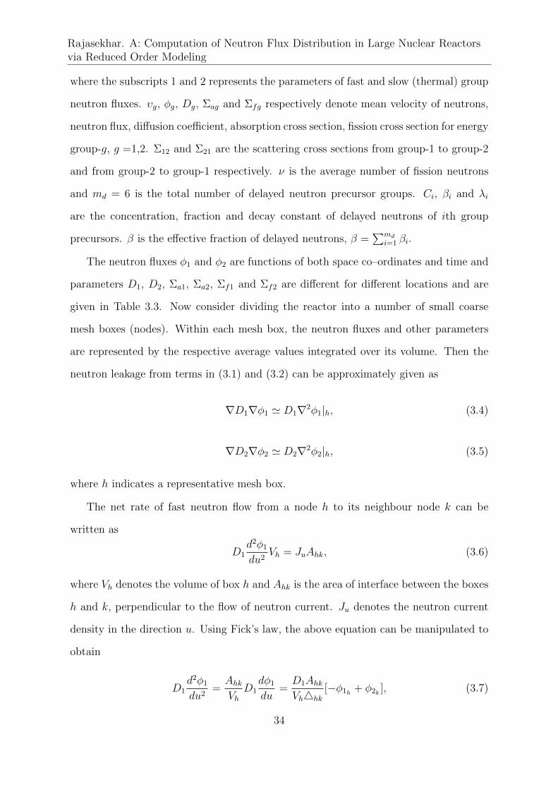
Rajasekhar. A: Computation of Neutron Flux Distribution in Large Nuclear Reactorsvia Reduced Order Modeling
where the subscripts 1 and 2 represents the parameters of fast and slow (thermal) group
neutron fluxes. υg, φg, Dg, Σag and Σfg respectively denote mean velocity of neutrons,
neutron flux, diffusion coefficient, absorption cross section, fission cross section for energy
group-g, g =1,2. Σ12 and Σ21 are the scattering cross sections from group-1 to group-2
and from group-2 to group-1 respectively. ν is the average number of fission neutrons
and md = 6 is the total number of delayed neutron precursor groups. Ci, βi and λi
are the concentration, fraction and decay constant of delayed neutrons of ith group
precursors. β is the effective fraction of delayed neutrons, β =∑md
i=1 βi.
The neutron fluxes φ1 and φ2 are functions of both space co–ordinates and time and
parameters D1, D2, Σa1, Σa2, Σf1 and Σf2 are different for different locations and are
given in Table 3.3. Now consider dividing the reactor into a number of small coarse
mesh boxes (nodes). Within each mesh box, the neutron fluxes and other parameters
are represented by the respective average values integrated over its volume. Then the
neutron leakage from terms in (3.1) and (3.2) can be approximately given as
∇D1∇φ1 ' D1∇2φ1|h, (3.4)
∇D2∇φ2 ' D2∇2φ2|h, (3.5)
where h indicates a representative mesh box.
The net rate of fast neutron flow from a node h to its neighbour node k can be
written as
D1d2φ1
du2Vh = JuAhk, (3.6)
where Vh denotes the volume of box h and Ahk is the area of interface between the boxes
h and k, perpendicular to the flow of neutron current. Ju denotes the neutron current
density in the direction u. Using Fick’s law, the above equation can be manipulated to
obtain
D1d2φ1
du2=AhkVh
D1dφ1
du=D1AhkVh4hk
[−φ1h + φ2k ], (3.7)
34
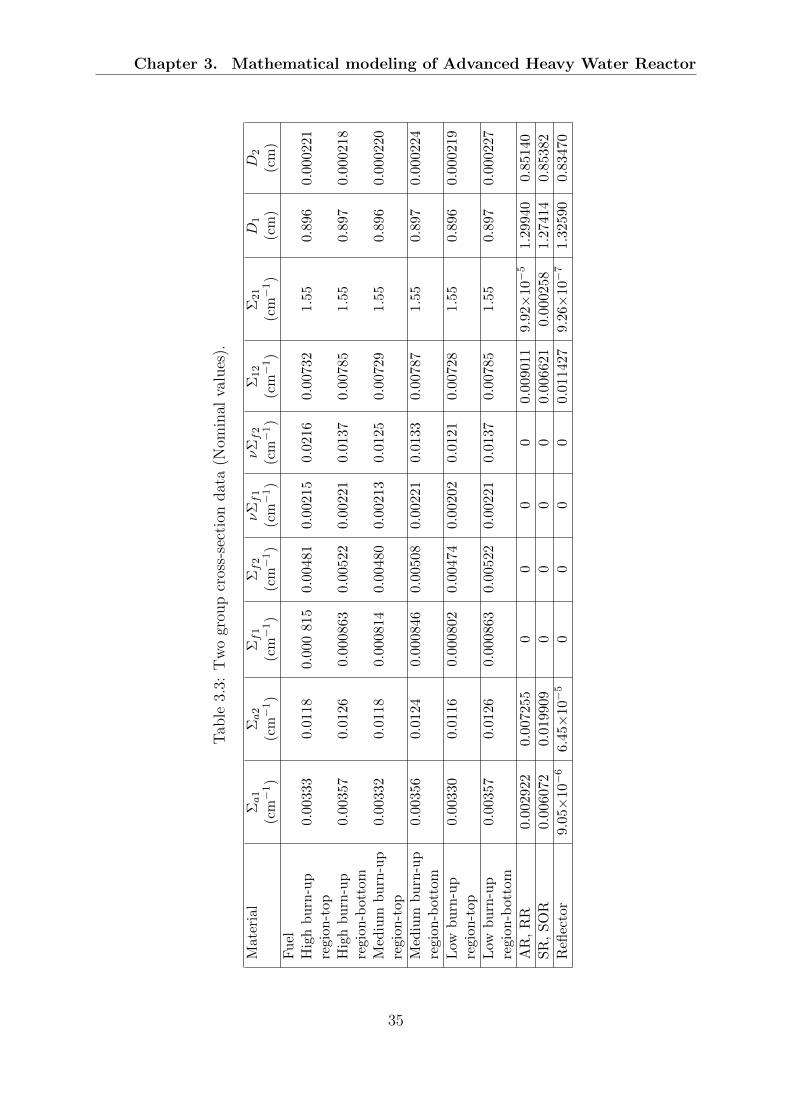
Chapter 3. Mathematical modeling of Advanced Heavy Water Reactor
Tab
le3.
3:T
wo
grou
pcr
oss-
sect
ion
dat
a(N
omin
alva
lues
).
Mate
rial
Σa1
Σa2
Σf1
Σf2
νΣf1
νΣf2
Σ12
Σ21
D1
D2
(cm−1)
(cm−1)
(cm−1)
(cm−1)
(cm−1)
(cm−1)
(cm−1)
(cm−1)
(cm
)(c
m)
Fu
elH
igh
bu
rn-u
p0.
00333
0.01
18
0.00
081
50.
0048
10.
0021
50.
0216
0.007
321.
55
0.896
0.000
221
regio
n-t
opH
igh
bu
rn-u
p0.
00357
0.01
26
0.00
0863
0.00
522
0.00
221
0.01
370.0
078
51.5
50.8
97
0.0
002
18re
gio
n-b
ott
om
Med
ium
bu
rn-u
p0.
00332
0.0
118
0.00
0814
0.00
480
0.00
213
0.01
250.0
072
91.5
50.8
96
0.0
002
20re
gio
n-t
op
Med
ium
bu
rn-u
p0.
00356
0.0
124
0.00
0846
0.00
508
0.00
221
0.01
330.0
078
71.5
50.8
97
0.0
002
24re
gio
n-b
ott
om
Low
bu
rn-u
p0.0
0330
0.01
16
0.00
0802
0.00
474
0.00
202
0.01
21
0.007
281.
550.
896
0.0
002
19re
gio
n-t
op
Low
bu
rn-u
p0.0
0357
0.01
26
0.00
0863
0.00
522
0.00
221
0.01
37
0.007
851.
550.
897
0.0
002
27re
gio
n-b
ott
om
AR
,R
R0.
002922
0.00
7255
00
00
0.009
011
9.9
2×
10−5
1.2
994
00.
851
40
SR
,S
OR
0.0
060
72
0.0
19909
00
00
0.0
066
210.0
002
581.2
741
40.
853
82
Refl
ecto
r9.
05×
10−6
6.45×
10−
50
00
00.
011
427
9.2
6×
10−7
1.3
259
00.
834
70
35

Rajasekhar. A: Computation of Neutron Flux Distribution in Large Nuclear Reactorsvia Reduced Order Modeling
where 4hk denotes the centre to the centre distance between the two nodes. Based on
the above, an approximation for the leakage terms in (3.4) and (3.5) could be
D1∇2φ1|h = −ω1hhφ1h +
Nh∑k=1
ω1hkφ1k, (3.8)
D2∇2φ2|h = −ω2hhφ2h +
Nh∑k=1
ω2hkφ2k, (3.9)
where
ωghk =DgAhkVh4hk
and ωghh =
Nh∑k=1
ωghk, g = 1, 2, (3.10)
and Nh is the total number of neighboring nodes to Node h. Substituting (3.7) to (3.9)
in (3.1) and (3.2), we have
1
υ1h
∂φ1h
∂t= −ω1hhφ1h +
Nh∑k=1
ω1hkφ1k − (Σa1hφ1h + Σ12hφ1h)
+Σ21φ2 + (1− β)(νΣf1hφ1h + νΣf2hφ2h) +
md∑i=1
λiCi, (3.11)
1
υ2h
∂φ2h
∂t= −ω2hhφ2h +
Nh∑k=1
ω2hkφ2k − Σa2hφ2h + Σ12hφ1h − Σ21φ2. (3.12)
Adding (3.11) and (3.12), and defining one group flux φh = φ1h + φ2h,
ωhh =ω1hh + ω2hhRh
(1 +Rh); ωhk =
ω1hk + ω2hkRh
(1 +Rh); Σah =
Σa1h + Σa2hRh
(1 +Rh); (3.13)
Σfh =Σf1h + Σf2hRh
(1 +Rh); vh =
(1 +Rh)1v1
+ Rh
v2
; Rh =φ2h
φ1h
(3.14)
we get
1
υh
∂φh∂t
= −ωhhφh +
Nh∑k=1
ωhkφk − Σahφh + (1− β)νφhΣfh +
md∑i=1
λiCi, (3.15)
36
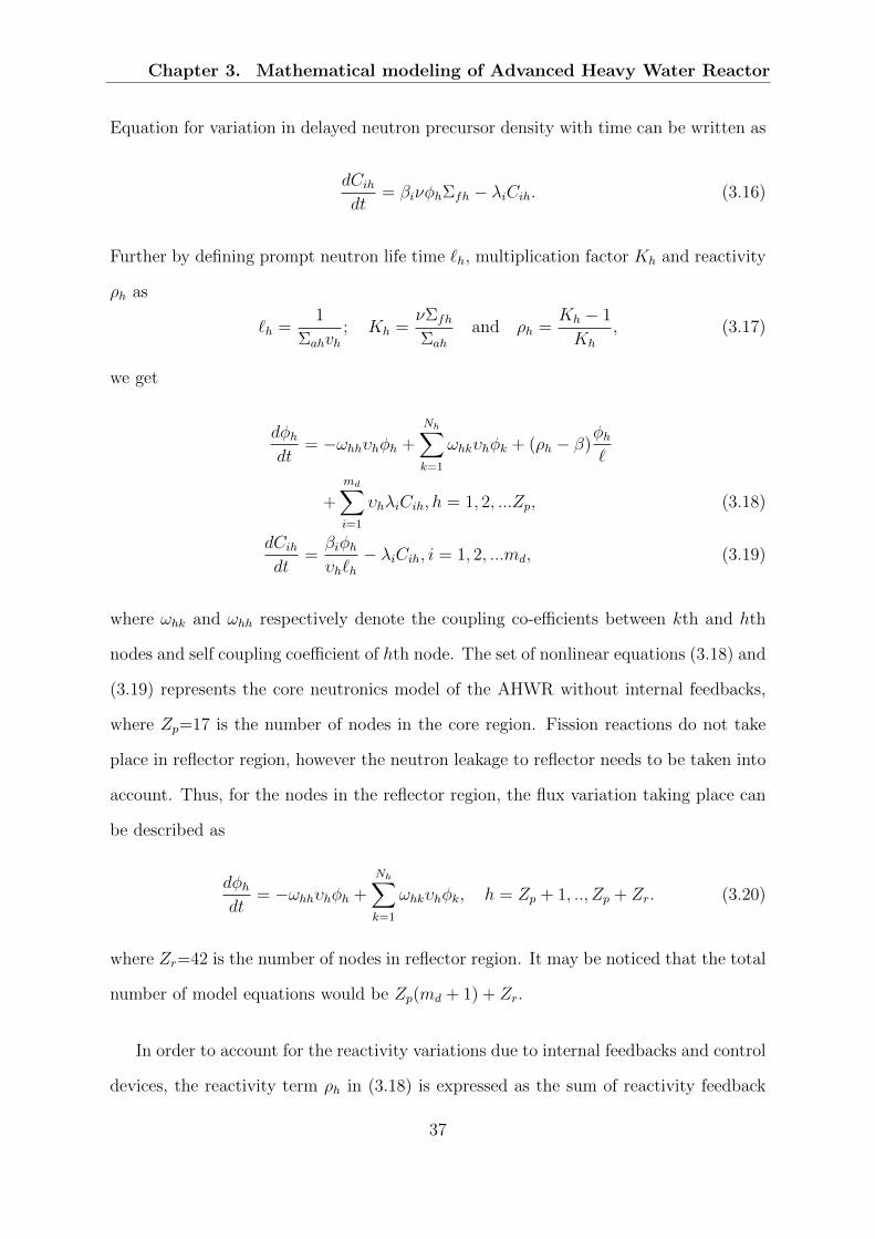
Chapter 3. Mathematical modeling of Advanced Heavy Water Reactor
Equation for variation in delayed neutron precursor density with time can be written as
dCihdt
= βiνφhΣfh − λiCih. (3.16)
Further by defining prompt neutron life time `h, multiplication factor Kh and reactivity
ρh as
`h =1
Σahvh; Kh =
νΣfh
Σah
and ρh =Kh − 1
Kh
, (3.17)
we get
dφhdt
= −ωhhυhφh +
Nh∑k=1
ωhkυhφk + (ρh − β)φh`
+
md∑i=1
υhλiCih, h = 1, 2, ...Zp, (3.18)
dCihdt
=βiφhυh`h
− λiCih, i = 1, 2, ...md, (3.19)
where ωhk and ωhh respectively denote the coupling co-efficients between kth and hth
nodes and self coupling coefficient of hth node. The set of nonlinear equations (3.18) and
(3.19) represents the core neutronics model of the AHWR without internal feedbacks,
where Zp=17 is the number of nodes in the core region. Fission reactions do not take
place in reflector region, however the neutron leakage to reflector needs to be taken into
account. Thus, for the nodes in the reflector region, the flux variation taking place can
be described as
dφhdt
= −ωhhυhφh +
Nh∑k=1
ωhkυhφk, h = Zp + 1, .., Zp + Zr. (3.20)
where Zr=42 is the number of nodes in reflector region. It may be noticed that the total
number of model equations would be Zp(md + 1) + Zr.
In order to account for the reactivity variations due to internal feedbacks and control
devices, the reactivity term ρh in (3.18) is expressed as the sum of reactivity feedback
37
Rajasekhar. A: Computation of Neutron Flux Distribution in Large Nuclear Reactorsvia Reduced Order Modeling
due to xenon and reactivity due to control rods, i.e., ρh = ρhx + ρhu. Other factors for
reactivity contribution such as fuel, coolant and moderator temperature are ignored due
to their less significance.
Benchmark problems and their reference solutions are available for Light Water Reac-
tors and PHWRs. These are useful for validation of simplified models. For the AHWR,
however, such benchmarks are not available. Therefore, for validation of simplified
space–time kinetics model and for validation of flux mapping algorithm a high fidelity
model is required. It is generally expected that a scheme with a very large number of
nodes will reproduce the flux distribution of the reactor core with good accuracy, and
at the same time it will also capture all the essential properties of the reactor, but the
model order will be correspondingly very large. Using (3.18)–(3.22) alongwith the 128-
node scheme as shown in Fig 3.4, a nonlinear stringent model has been developed for
validation purpose. In the 128-node scheme, the core region, top reflector region, and
bottom reflector region each are divided into 128 nodes. The side reflector region is di-
vided into eight nodes, giving 392 nodes in all. It may be noticed that the total mumber
of model equations would be 1168 resulting into 1168th order model, since Zp = 128 and
Zr = 264.
The physical parameters such as volume of the nodes, area of interface, distance
between the nodes, and the homogenized neutron cross-sections for the nodes under
consideration are essential for computation of coupling coefficients and determination of
the estimation model. The average coolant densities in the bottom half (for a length of
1.75 m from the core bottom) and top half (remaining 1.75 m length of the lattices) of
the reactor core under full power operating conditions are calculated as 0.74 g/cc and
0.45 g/cc respectively, and corresponding cross sections given in Table 3.3 are used in
the analysis. The delayed neutron data of the AHWR are given in Table 3.4.
38
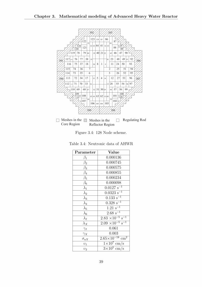
Chapter 3. Mathematical modeling of Advanced Heavy Water Reactor
Figure 3.4: 128 Node scheme.
Table 3.4: Neutronic data of AHWR
Parameter Valueβ1 0.000136β2 0.000745β3 0.000575β4 0.000855β5 0.000234β6 0.000098λ1 0.0127 s−1
λ2 0.0323 s−1
λ3 0.133 s−1
λ4 0.328 s−1
λ5 1.21 s−1
λ6 2.68 s−1
λI 2.83 ×10⁻⁵ s−1
λX 2.09 ×10−5 s−1
γI 0.061γX 0.003σaX 2.65×10−18 cm2
υ1 1×107 cm/sυ2 3×105 cm/s
39
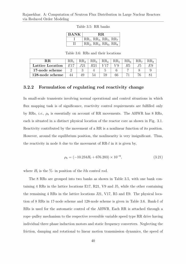
Rajasekhar. A: Computation of Neutron Flux Distribution in Large Nuclear Reactorsvia Reduced Order Modeling
Table 3.5: RR banks
BANK RRI RR1, RR3, RR5, RR7
II RR2, RR4, RR6, RR8
Table 3.6: RRs and their locations
RR RR1 RR2 RR3 RR4 RR5 RR6 RR7 RR8
Lattice Location E17 J21 R21 V 17 V 9 R5 J5 E917-node scheme 2 3 4 5 6 7 8 9128-node scheme 44 49 54 59 66 71 76 81
3.2.2 Formulation of regulating rod reactivity change
In small-scale transients involving normal operational and control situations in which
flux mapping task is of significance, reactivity control requirements are fulfilled only
by RRs, i.e., ρh is essentially on account of RR movements. The AHWR has 8 RRs,
each is situated in a distinct physical location of the reactor core as shown in Fig. 3.1.
Reactivity contributed by the movement of a RR is a nonlinear function of its position.
However, around the equilibrium position, the nonlinearity is very insignificant. Thus,
the reactivity in node h due to the movement of RR-l in it is given by,
ρh = (−10.234Hl + 676.203)× 10−6, (3.21)
where Hl is the %- in position of the lth control rod.
The 8 RRs are grouped into two banks as shown in Table 3.5, with one bank con-
taining 4 RRs in the lattice locations E17, R21, V9 and J5, while the other containing
the remaining 4 RRs in the lattice locations J21, V17, R5 and E9. The physical loca-
tion of 8 RRs in 17-node scheme and 128-node scheme is given in Table 3.6. Bank-I of
RRs is used for the automatic control of the AHWR. Each RR is attached through a
rope–pulley mechanism to the respective reversible variable speed type RR drive having
individual three phase induction motors and static frequency converters. Neglecting the
friction, damping and rotational to linear motion transmission dynamics, the speed of
40
Chapter 3. Mathematical modeling of Advanced Heavy Water Reactor
the regulating rod is directly proportional to the applied voltage ϑl to the drive motor,
i.e.,
dHl
dt= KRRϑl, l = 1, ..., 8, (3.22)
where ϑl is the control signal. It is in the range of ±1V and KRR = 0.56, a constant.
3.2.3 Formulation of Xenon reactivity feedback
Iodine and xenon dynamics in each node h in the core region can be described as
dIhdt
= γIΣfhφh − λIIh, (3.23)
dXh
dt= γXΣfhφh + λIIh − (λX + σaXφh)Xh, (3.24)
where Ih and Xh denote iodine and xenon concentrations respectively in node h, γI and
γX are their respective fractional yields, and λI and λX are respective decay constants.
The xenon reactivity feedback in a node h is given by
ρhX =σaXXh
Σah
. (3.25)
3.3 Steady–state Neutron Flux Distribution
For the study presented in this thesis, steady–state reference flux distributions are gen-
erated using finite-difference method (FDM) as described in [88]. Active core region of
the AHWR alongwith reflector region is considered to be divided in fine meshes. Each
channel in the core region is vertically divided into 24 mesh boxes making the reactor
core into 12, 312 meshes, with 24 meshes along the reactor axis. The side, top and
bottom reflector regions are assumed to be divided into 6048, 2295 and 2295 non-power
generating meshes respectively. Therefore, core including reflector is assumed to be di-
vided into 765 vertical sections and 30 horizontal planes, such that 30 meshes are along
41
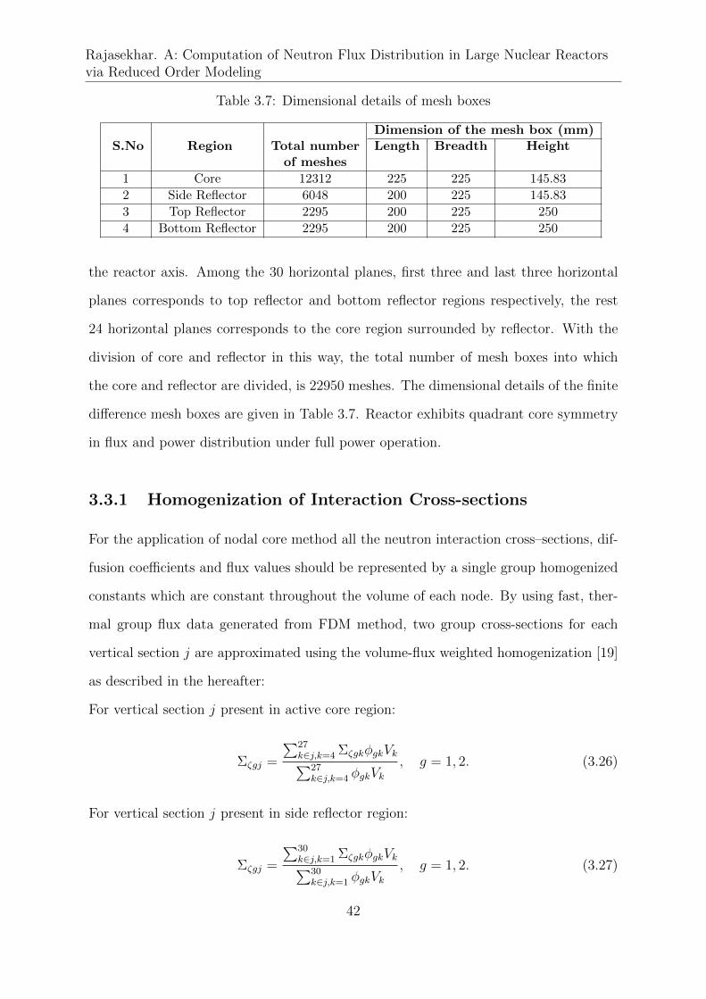
Rajasekhar. A: Computation of Neutron Flux Distribution in Large Nuclear Reactorsvia Reduced Order Modeling
Table 3.7: Dimensional details of mesh boxes
S.NoDimension of the mesh box (mm)
Region Total number Length Breadth Heightof meshes
1 Core 12312 225 225 145.83
2 Side Reflector 6048 200 225 145.83
3 Top Reflector 2295 200 225 250
4 Bottom Reflector 2295 200 225 250
the reactor axis. Among the 30 horizontal planes, first three and last three horizontal
planes corresponds to top reflector and bottom reflector regions respectively, the rest
24 horizontal planes corresponds to the core region surrounded by reflector. With the
division of core and reflector in this way, the total number of mesh boxes into which
the core and reflector are divided, is 22950 meshes. The dimensional details of the finite
difference mesh boxes are given in Table 3.7. Reactor exhibits quadrant core symmetry
in flux and power distribution under full power operation.
3.3.1 Homogenization of Interaction Cross-sections
For the application of nodal core method all the neutron interaction cross–sections, dif-
fusion coefficients and flux values should be represented by a single group homogenized
constants which are constant throughout the volume of each node. By using fast, ther-
mal group flux data generated from FDM method, two group cross-sections for each
vertical section j are approximated using the volume-flux weighted homogenization [19]
as described in the hereafter:
For vertical section j present in active core region:
Σζgj =
∑27k∈j,k=4 ΣζgkφgkVk∑27
k∈j,k=4 φgkVk, g = 1, 2. (3.26)
For vertical section j present in side reflector region:
Σζgj =
∑30k∈j,k=1 ΣζgkφgkVk∑30
k∈j,k=1 φgkVk, g = 1, 2. (3.27)
42
Chapter 3. Mathematical modeling of Advanced Heavy Water Reactor
For vertical section j present in top reflector region:
Σζgj =
∑3k∈j,k=1 ΣζgkφgkVk∑3
k∈j,k=1 φgkVk, g = 1, 2. (3.28)
For vertical section j present in bottom reflector region:
Σζgj =
∑30k∈j,k=28 ΣζgkφgkVk∑30
k∈j,k=28 φgkVk, g = 1, 2. (3.29)
The group-wise homogenized constants of each node h were computed using
Σζgh =
∑∀j∈h ΣζgjφgjVj∑∀j∈h φgjVj
, g = 1, 2; h = 1, 2, ..., Zr. (3.30)
where Σ denotes the cross section, ζ denotes a neutron interaction and j denotes the
vertical section indices in the reactor core. k denotes the index of the mesh box and
it runs from 1 to 3, 4 to 27, 28 to 30 and 1 to 30 for vertical sections of top reflector,
active core, bottom reflector and side reflector regions respectively. The steady-state
equivalent mesh box fluxes were calculated by adding the two group flux data generated
from FDM computations and is given by
φm0 = φ01m + φ0
2m, (3.31)
where φ01m and φ0
2m are the volume weighted homogenized fluxes in mesh box m, for the
fast and thermal groups respectively. The steady–state equivalent flux in the vertical
section j obtained from the fast and thermal energy groups is given by
φj0 = φ01j + φ0
2j, (3.32)
where φ01j and φ0
2j are the volume weighted homogenized fluxes in vertical section j, for
the fast and thermal groups respectively. The steady–state equivalent flux in node h
43
Rajasekhar. A: Computation of Neutron Flux Distribution in Large Nuclear Reactorsvia Reduced Order Modeling
obtained from both the fast and thermal energy groups is given by
φh0 = φ01h + φ0
2h, (3.33)
where φ01h and φ0
2h are the volume weighted homogenized fluxes in node h, for the fast
and thermal groups respectively.
3.4 Reconstruction of 3-D Neutron Flux Distribu-
tion
Nodal methods have a fundamental limitation as they fail to predict the detailed flux
shapes throughout the reactor core. Of course, such detailed information can be of vital
importance in the course of designing and operation of the reactor. The methods for de-
veloping homogenized parameters for large nodes from detailed heterogeneous solutions
and the problem of deriving local pin powers from the nodal solutions are generally ap-
plied to time–independent problems. The pin-by-pin flux distribution within each node
is calculated using a de-homogenization method or Flux Reconstruction Method (FRM)
[101] from nodal solutions. This method is superior than FDM in view of computational
time and it is based on the assumption that the fine-mesh point flux can be expressed
as the product of flux of the assembly to which it belongs, which is obtained through
a vertical grid level weighting factor applied on the global flux, and a mesh box level
weighting factor corresponding to it.
From (3.32) and (3.33), the weighting factor for each vertical section j in a node h
is given by κj = φj0/φh0. The weighting factor for each mesh box m in any vertical grid
j can be found from the axial flux distribution obtained from the steady–state FDM
computation. The weighting factor for each mesh box m in a vertical grid j is defined
as κjm = φjm0/φj0. During the transient, the fluxes in vertical grids and mesh boxes
vary according to the transient value of the nodal flux and weighting factors κj and κjm
44
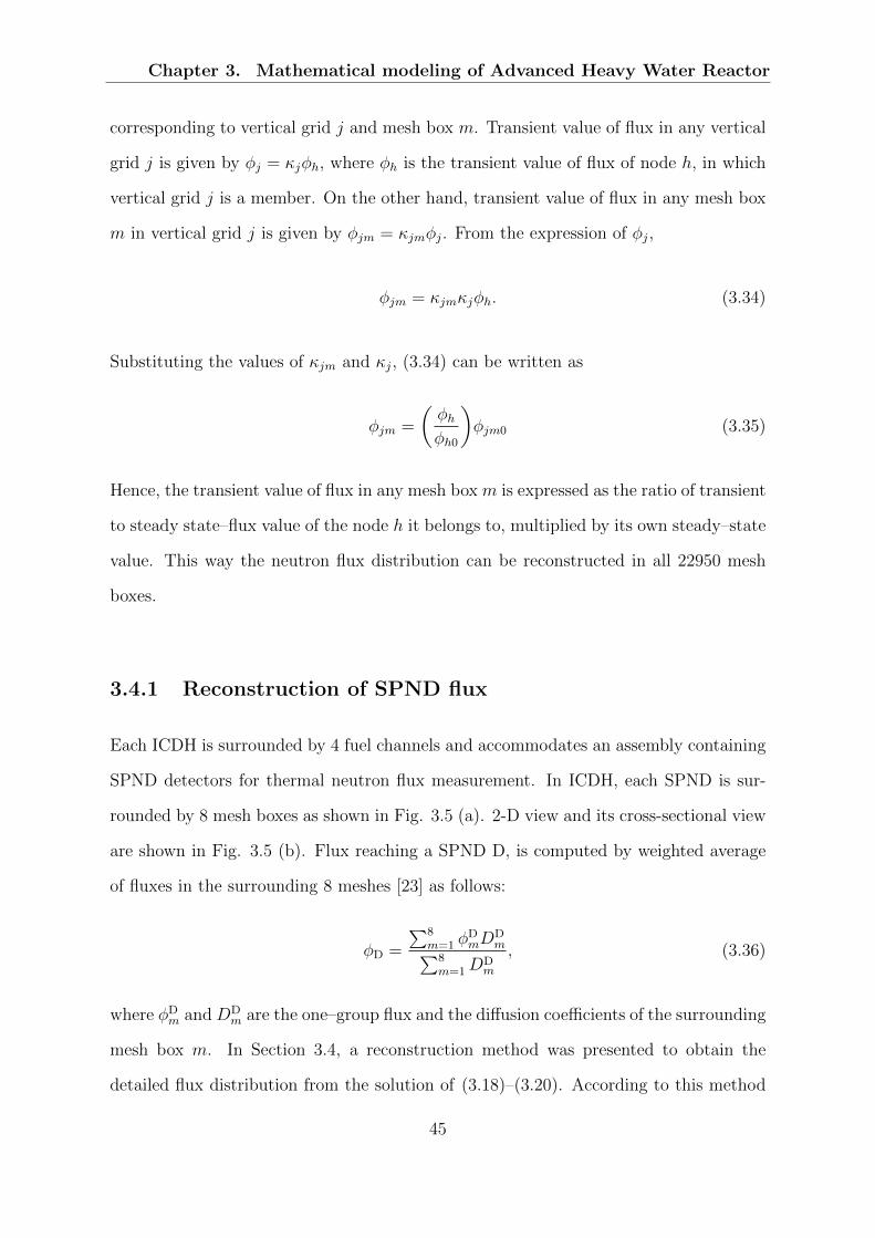
Chapter 3. Mathematical modeling of Advanced Heavy Water Reactor
corresponding to vertical grid j and mesh box m. Transient value of flux in any vertical
grid j is given by φj = κjφh, where φh is the transient value of flux of node h, in which
vertical grid j is a member. On the other hand, transient value of flux in any mesh box
m in vertical grid j is given by φjm = κjmφj. From the expression of φj,
φjm = κjmκjφh. (3.34)
Substituting the values of κjm and κj, (3.34) can be written as
φjm =
(φhφh0
)φjm0 (3.35)
Hence, the transient value of flux in any mesh box m is expressed as the ratio of transient
to steady state–flux value of the node h it belongs to, multiplied by its own steady–state
value. This way the neutron flux distribution can be reconstructed in all 22950 mesh
boxes.
3.4.1 Reconstruction of SPND flux
Each ICDH is surrounded by 4 fuel channels and accommodates an assembly containing
SPND detectors for thermal neutron flux measurement. In ICDH, each SPND is sur-
rounded by 8 mesh boxes as shown in Fig. 3.5 (a). 2-D view and its cross-sectional view
are shown in Fig. 3.5 (b). Flux reaching a SPND D, is computed by weighted average
of fluxes in the surrounding 8 meshes [23] as follows:
φD =
∑8m=1 φ
DmD
Dm∑8
m=1DDm
, (3.36)
where φDm and DD
m are the one–group flux and the diffusion coefficients of the surrounding
mesh box m. In Section 3.4, a reconstruction method was presented to obtain the
detailed flux distribution from the solution of (3.18)–(3.20). According to this method
45
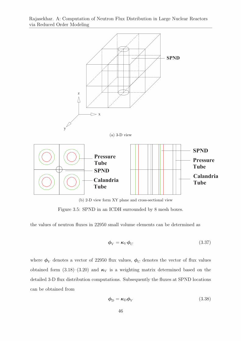
Rajasekhar. A: Computation of Neutron Flux Distribution in Large Nuclear Reactorsvia Reduced Order Modeling
(a) 3-D view
(b) 2-D view form XY plane and cross-sectional view
Figure 3.5: SPND in an ICDH surrounded by 8 mesh boxes.
the values of neutron fluxes in 22950 small volume elements can be determined as
φV = κVφC (3.37)
where φV denotes a vector of 22950 flux values, φC denotes the vector of flux values
obtained form (3.18)–(3.20) and κV is a weighting matrix determined based on the
detailed 3-D flux distribution computations. Subsequently the fluxes at SPND locations
can be obtained from
φD = κDφV (3.38)
46
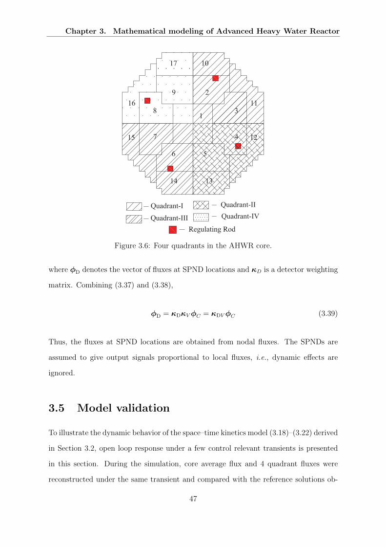
Chapter 3. Mathematical modeling of Advanced Heavy Water Reactor
Figure 3.6: Four quadrants in the AHWR core.
where φD denotes the vector of fluxes at SPND locations and κD is a detector weighting
matrix. Combining (3.37) and (3.38),
φD = κDκVφC = κDVφC (3.39)
Thus, the fluxes at SPND locations are obtained from nodal fluxes. The SPNDs are
assumed to give output signals proportional to local fluxes, i.e., dynamic effects are
ignored.
3.5 Model validation
To illustrate the dynamic behavior of the space–time kinetics model (3.18)–(3.22) derived
in Section 3.2, open loop response under a few control relevant transients is presented
in this section. During the simulation, core average flux and 4 quadrant fluxes were
reconstructed under the same transient and compared with the reference solutions ob-
47

Rajasekhar. A: Computation of Neutron Flux Distribution in Large Nuclear Reactorsvia Reduced Order Modeling
tained from a separate set of computations using a 128 node scheme as shown in Fig.
3.4. The four quadrant scheme of AHWR is shown in Fig 3.6. The quadrant and core
average fluxes, from the nodal solutions, were computed using reconstruction technique
as described in Section 3.4. It is as follows: quadrant fluxes are obtained as an average
of all the mesh box fluxes in each quadrant; and the core average flux is computed as
the average of all the quadrant fluxes. To characterize the accuracy of the model, the
error in core-average and quadrant fluxes is computed using,
eφi = (φiref − φi)× 100, i = I, II, III, IV, (3.40)
where φiref denotes the reference value of neutron flux in quadrant i and φi denotes the
neutron flux in quadrant i.
Initially, the reactor was assumed to be operating on full power. It was also assumed
that initially each RR is equally at 66.7% in position, ARs are fully in and SRs and
shut-off rods are fully out, which is the critical configuration of the equilibrium core of
AHWR. For a control voltage with positive magnitude, the corresponding RR moves into
the core and for a negative control voltage, it moves out of the core. The regulating rod
is stationary when the control voltage applied to it is zero. The transients are described
in the following subsections. In each case, the reactor is at steady–state for the initial
50 seconds.
3.5.1 Case I: Movement of RR in Quadrant–I
This simulation involves movement of RR located in Quadrant-I. At time t = 50 s,
control signal of 1 V is applied to RR drive and maintained for 8 s. Corresponding
RR moves linearly into the reactor core, as governed by (3.22) and reaches 71.14% in
position. Then, control signal is made 0 V to hold the RR at the new position. After
3 s, the RR is driven out linearly to nominal position by applying a control signal of
−1 V. Again after 3 s, an outward movement followed by inward movement back to its
48

Chapter 3. Mathematical modeling of Advanced Heavy Water Reactor
0 10 20 30 40 50 60 70 80 90 100 110 120−1.5
−1
−0.5
0
0.5
1
1.5
Con
trol
Vol
tage
(V
)
Time (s)0 10 20 30 40 50 60 70 80 90 100 110 120
60
62
64
66
68
70
72
RR
Pos
ition
(%
in )
Control voltage
RR position
Figure 3.7: Position of RR corresponding to applied control signal.
nominal position is simulated.
Fig. 3.7 shows the applied control voltage to RR drive and corresponding position
of the RR in the core during the applied transient. Fig. 3.8 shows the core average flux
alongwith error in core average flux computed using nodal method, taking computations
from 128 node scheme as reference. Fig. 3.9 and Fig. 3.10 show the average values of
flux in Quadrants-I, II, III and IV of the reactor alongwith error.
3.5.2 Case II: Differential Movement of 2 RRs
Scenarios in which the flux/power distribution in the reactor core undergoes variations,
despite of the total power remaining constant are of great significance in spatial reactor
control applications. In order to assess the validity of the space–time kinetics model
under such conditions, a transient involving simultaneous counter-movement of two di-
agonally opposite RRs was simulated. At time t=50 s, the RR in Quadrant-III was
driven linearly into the reactor core from its nominal position under a signal of 1 V,
while the RR at the diagonally opposite lattice location in Quadrant-I was driven out
simultaneously at the same speed under a signal of −1 V. Fig. 3.11 shows the position
of RRs in the core during the applied transient.
Fig. 3.12 shows the core average flux alongwith error in core average flux computed
using nodal method, taking computations from 128 node scheme as reference. Fig. 3.13
49
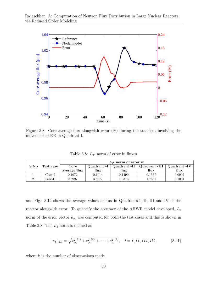
Rajasekhar. A: Computation of Neutron Flux Distribution in Large Nuclear Reactorsvia Reduced Order Modeling
0 20 40 60 80 100 1200.94
0.96
0.98
1
1.02
1.04C
ore
aver
age
flux
(p.u
)
Time (s)
0 20 40 60 80 100 120−0.12
−0.06
0
0.06
0.12
0.18
0.24
Err
or (
%)
ReferenceNodal modelError
Figure 3.8: Core average flux alongwith error (%) during the transient involving themovement of RR in Quadrant-I.
Table 3.8: L2- norm of error in fluxes
S.NoL2- norm of error in
Test case Core Quadrant -I Quadrant -II Quadrant -III Quadrant -IVaverage flux flux flux flux flux
1 Case-I 0.1072 0.1014 0.1490 0.1557 0.09072 Case-II 2.5997 3.6277 1.9373 1.7581 3.1031
and Fig. 3.14 shows the average values of flux in Quadrants-I, II, III and IV of the
reactor alongwith error. To quantify the accuracy of the AHWR model developed, L2
norm of the error vector eφi was computed for both the test cases and this is shown in
Table 3.8. The L2 norm is defined as
|eφi |L2 =
√e2φi
(1)+ e2φi
(2)+ · · ·+ e2φi
(k), i = I, II, III, IV, (3.41)
where k is the number of observations made.
50

Chapter 3. Mathematical modeling of Advanced Heavy Water Reactor
0 20 40 60 80 100 1200.94
0.96
0.98
1
1.02
1.04A
vera
ge fl
ux in
Qua
dran
t−I (
p.u)
Time (s)
0 20 40 60 80 100 120−0.12
−0.06
0
0.06
0.12
0.18
0.24
Err
or (
%)
ReferenceNodal modelError
0 20 40 60 80 100 1200.94
0.96
0.98
1
1.02
1.04
Ave
rage
flux
in Q
uadr
ant−
II (p
.u)
Time (s)
0 20 40 60 80 100 120−0.1
0
0.1
0.2
0.3
Err
or (
%)
ReferenceNodal modelError
Figure 3.9: Average flux in Quadrants I and II during the movement of RR in quadrantI.
51
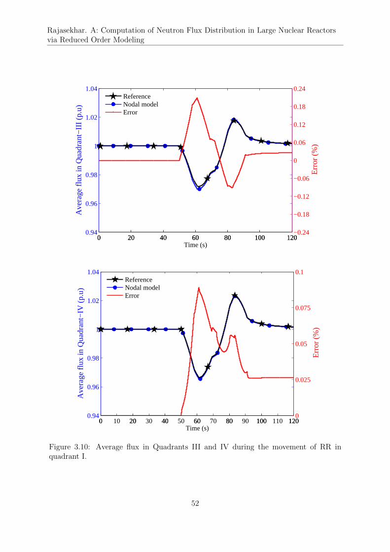
Rajasekhar. A: Computation of Neutron Flux Distribution in Large Nuclear Reactorsvia Reduced Order Modeling
0 20 40 60 80 100 1200.94
0.96
0.98
1
1.02
1.04
Ave
rage
flux
in Q
uadr
ant−
III (
p.u)
Time (s)
0 20 40 60 80 100 120−0.24
−0.18
−0.12
−0.06
0
0.06
0.12
0.18
0.24
Err
or (
%)
ReferenceNodal modelError
0 20 40 60 80 100 1200.94
0.96
0.98
1
1.02
1.04
Ave
rage
flux
in Q
uadr
ant−
IV (
p.u)
Time (s)
0 10 20 30 40 50 60 70 80 90 100 110 1200
0.025
0.05
0.075
0.1
Err
or (
%)
ReferenceNodal modelError
Figure 3.10: Average flux in Quadrants III and IV during the movement of RR inquadrant I.
52

Chapter 3. Mathematical modeling of Advanced Heavy Water Reactor
0 20 40 60 80 100 12020
40
60
80
100
Time (s)
RR
pos
ition
(%
in)
RR in Quadrant−IRR in Quadrant−III
Figure 3.11: Position of RRs in Quadrant-I and Quadrant-III during the transient in-volving differential movement of RRs.
0 20 40 60 80 100 1200.95
1
1.05
1.1
1.15
Cor
e av
erag
e flu
x (p
.u)
Time (s)
0 20 40 60 80 100 120−2
−1
0
1
2
3
4
Err
or (
%)
ReferenceNodal modelError
Figure 3.12: Core average flux alongwith error (%) during the transient involving dif-ferential movement of RRs.
53
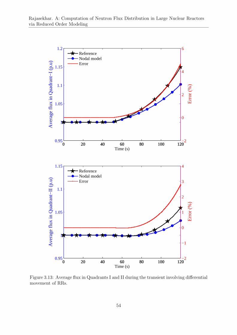
Rajasekhar. A: Computation of Neutron Flux Distribution in Large Nuclear Reactorsvia Reduced Order Modeling
0 20 40 60 80 100 1200.95
1
1.05
1.1
1.15
1.2A
vera
ge fl
ux in
Qua
dran
t−I (
p.u)
Time (s)
0 20 40 60 80 100 120−2
0
2
4
6
Err
or (
%)
ReferenceNodal modelError
0 20 40 60 80 100 1200.95
1
1.05
1.1
1.15
Ave
rage
flux
in Q
uadr
ant−
II (p
.u)
Time (s)
0 20 40 60 80 100 120−2
−1
0
1
2
3
4
Err
or (
%)
ReferenceNodal modelError
Figure 3.13: Average flux in Quadrants I and II during the transient involving differentialmovement of RRs.
54
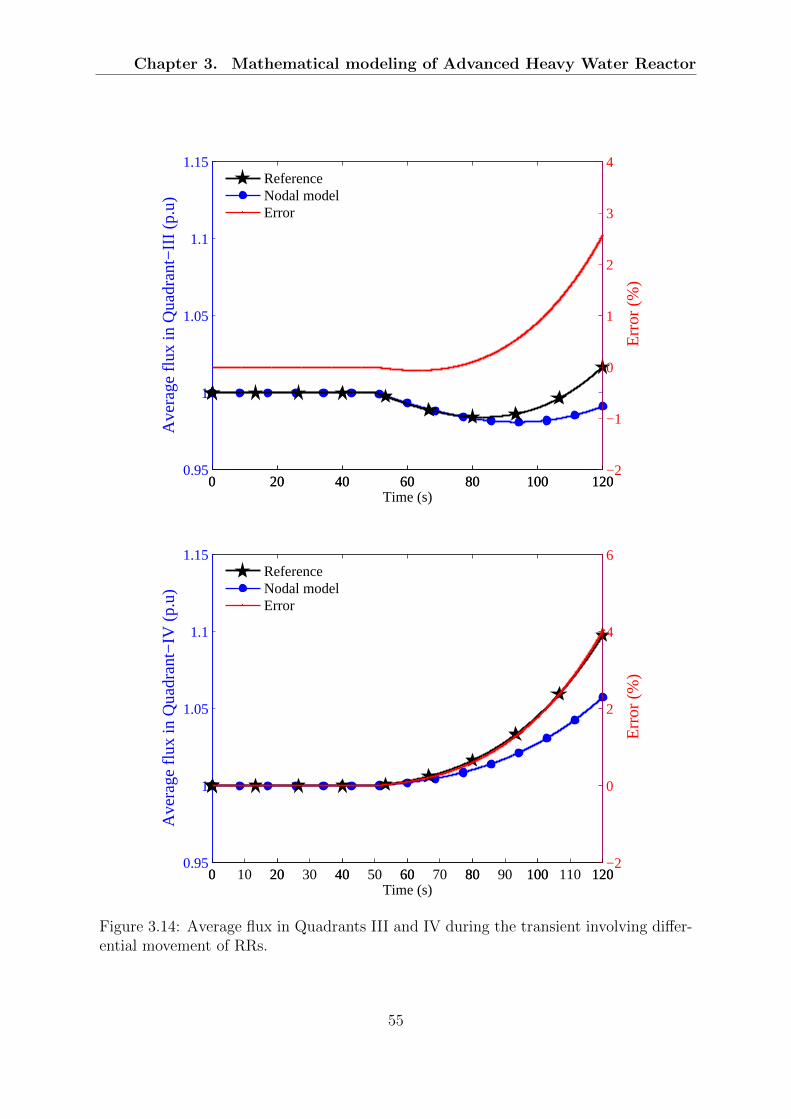
Chapter 3. Mathematical modeling of Advanced Heavy Water Reactor
0 20 40 60 80 100 1200.95
1
1.05
1.1
1.15A
vera
ge fl
ux in
Qua
dran
t−III
(p.
u)
Time (s)
0 20 40 60 80 100 120−2
−1
0
1
2
3
4
Err
or (
%)
ReferenceNodal modelError
0 20 40 60 80 100 1200.95
1
1.05
1.1
1.15
Ave
rage
flux
in Q
uadr
ant−
IV (
p.u)
Time (s)
0 10 20 30 40 50 60 70 80 90 100 110 120−2
0
2
4
6
Err
or (
%)
ReferenceNodal modelError
Figure 3.14: Average flux in Quadrants III and IV during the transient involving differ-ential movement of RRs.
55
Rajasekhar. A: Computation of Neutron Flux Distribution in Large Nuclear Reactorsvia Reduced Order Modeling
3.6 Discussion
In this chapter, a nonlinear dynamic model which represents time–dependent behavior
of AHWR has been presented. The dynamic behavior of the model has also been val-
idated for core average flux and Quadrant fluxes using a high fidelity model based on
128-node scheme of AHWR. From the simulations, it can be concluded that for a consid-
erable perturbation around the steady–state operating point, the core average flux and
reconstructed fluxes in all the quadrants from the AHWR model are found to be in good
agreement with the reference values. As a result of this, AHWR model with 128-node
scheme is suitable for generation of accurate detector fluxes which can be used as real
time plant data and reference model with 17-node scheme is suitable for estimation of
detailed flux distribution in the reactor core using Kalman filtering technique.
56
Chapter 4
Theory of Model Reduction
Techniques
Complex large–scale systems usually require high dimensional models to represent
them accurately. Analysis, simulation and design methods based on such high order
models may eventually lead to complicated control strategies requiring very complex
logic or large amounts of computation. The development of state–space methods has
made it feasible to design a control system for high order linear systems. When the order
of the system becomes very high, however, special algebraic techniques for performing
the design calculations are required to permit the calculations to be performed at a
reasonable cost in a typical digital computer. Moreover, a control system designed
for a very high order linear system is likely to be more complicated than it would
be reasonable to build. Because of their importance on systems analysis and in the
design of controllers or observers, model reduction methods have received considerable
attention over the past few decades. Among the various classes of model reduction
methods, modal techniques have gained significant interest since they permit explicit
formulation. i.e., the reduced order model is derived directly from the linear large–scale
Parts of this chapter were published in 2015 IEEE international Conference on Industrial Instru-mentation and Control Applications (ICIC), Pune, India and in Annals of Nuclear Energy, Vol. 102.
57
Rajasekhar. A: Computation of Neutron Flux Distribution in Large Nuclear Reactorsvia Reduced Order Modeling
system through algebraic relationships. This chapter presents the theory of some of
the model order reduction techniques viz. Davison’s, Marshall’s, singular perturbation
analysis and balanced truncation.
4.1 Formulation of Model Order Reduction Prob-
lem
Classic and modern control theories are usually concerned with analyzing and synthe-
sizing systems described by ordinary differential equations (ODE) that often represent
physical laws governing the dynamics of the given system. The linearization of higher
nonlinear ODEs about an equilibrium, leads to the well-known representation of a linear-
time invariant (LTI) system. Consider a large–scale dynamical system described by the
LTI model
x(t) = Ax(t) + Bu(t),
y(t) = Ψx(t),
(4.1)
where x(t) ∈ Rn, u(t) ∈ Rm, and y(t) ∈ Rp are the state, input and output vectors
respectively; A ∈ Rn×n, B ∈ Rn×m and Ψ ∈ Rp×n are system, input and output
matrices respectively. For the rest of this thesis, assume the notion of large–scale system
represented by (4.1) in state–space form as G :=
A B
Ψ 0
. The same G is also used
to denote the Transfer Function (TF) corresponding to (4.1). From the context there
would be no ambiguity. The transfer function from u to y is G(s) := Ψ (sI −A)−1B.
The order n of the LTI system ranges from a few tens to several hundred for large–scale
systems. The increase in dimension and the desire to control the multi-input/multi-
output systems triggered the need of application of model order reduction. The intent
of model order reduction is to obtain a simplified lower order, model which preserves
the input and output behavior of the system.
The reduced order model of order r < n, has the same response characteristics as
58
Chapter 4. Theory of Model Reduction Techniques
that of the original model with far less storage requirements and much lower evaluation
time. The resulting model given by,
xr(t) = Arxr(t) + Bru(t), (4.2)
yr(t) = Ψ rxr(t) (4.3)
might be used to replace the original description in simulation studies or it might be used
to design a reduced order controller or observer. The application of Davison’s technique,
Marshall’s technique, singular perturbation analysis and balanced truncation has been
explored in this thesis and these techniques are described briefly in the following sections.
4.2 Davison’s Technique
Davison [14] proposed one of the first structured approach to model order reduction.
It approximates the original order n of the system to r by neglecting the eigenvalues
of the original system that are farthest from the origin and retains only the dominant
eigenvalues and hence the dominant time constants of the original system are present
in the reduced order model. Initially the system states are rearranged in such a manner
that the eigenvectors corresponding to the states to be retained from (4.1) are placed
first.
The essence of this modal approach to model reduction consists of neglecting the
dynamics associated with fast modes, i.e., those which die out quickly when perturbed.
Hence, it is useful to partition the above relationships in terms of dominant and non-
dominant modes, as well as important and less important state variables. Let the
state vector x be partitioned into dominant and non-dominant parts as x1, which are
considered to be retained and x2, which are to be ignored. Therefore the partitioned
59
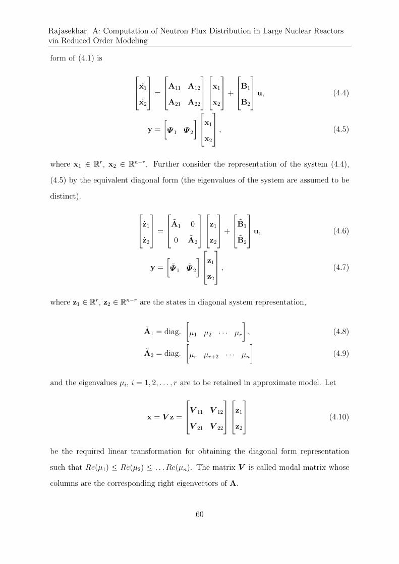
Rajasekhar. A: Computation of Neutron Flux Distribution in Large Nuclear Reactorsvia Reduced Order Modeling
form of (4.1) is
x1
x2
=
A11 A12
A21 A22
x1
x2
+
B1
B2
u, (4.4)
y =
[Ψ 1 Ψ 2
]x1
x2
, (4.5)
where x1 ∈ Rr, x2 ∈ Rn−r. Further consider the representation of the system (4.4),
(4.5) by the equivalent diagonal form (the eigenvalues of the system are assumed to be
distinct).
z1
z2
=
A1 0
0 A2
z1
z2
+
B1
B2
u, (4.6)
y =
[Ψ 1 Ψ 2
]z1
z2
, (4.7)
where z1 ∈ Rr, z2 ∈ Rn−r are the states in diagonal system representation,
A1 = diag.
[µ1 µ2 · · · µr
], (4.8)
A2 = diag.
[µr µr+2 · · · µn
](4.9)
and the eigenvalues µi, i = 1, 2, . . . , r are to be retained in approximate model. Let
x = V z =
V 11 V 12
V 21 V 22
z1
z2
(4.10)
be the required linear transformation for obtaining the diagonal form representation
such that Re(µ1) ≤ Re(µ2) ≤ . . . Re(µn). The matrix V is called modal matrix whose
columns are the corresponding right eigenvectors of A.
60
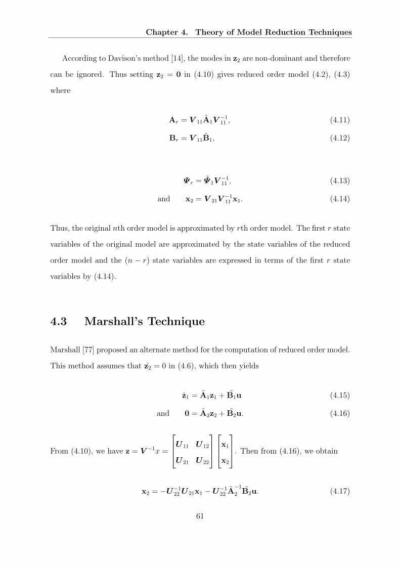
Chapter 4. Theory of Model Reduction Techniques
According to Davison’s method [14], the modes in z2 are non-dominant and therefore
can be ignored. Thus setting z2 = 0 in (4.10) gives reduced order model (4.2), (4.3)
where
Ar = V 11A1V−111 , (4.11)
Br = V 11B1, (4.12)
Ψ r = Ψ 1V−111 , (4.13)
and x2 = V 21V−111 x1. (4.14)
Thus, the original nth order model is approximated by rth order model. The first r state
variables of the original model are approximated by the state variables of the reduced
order model and the (n − r) state variables are expressed in terms of the first r state
variables by (4.14).
4.3 Marshall’s Technique
Marshall [77] proposed an alternate method for the computation of reduced order model.
This method assumes that z2 = 0 in (4.6), which then yields
z1 = A1z1 + B1u (4.15)
and 0 = A2z2 + B2u. (4.16)
From (4.10), we have z = V −1x =
U 11 U 12
U 21 U 22
x1
x2
. Then from (4.16), we obtain
x2 = −U−122U 21x1 −U−122 A−12 B2u. (4.17)
61
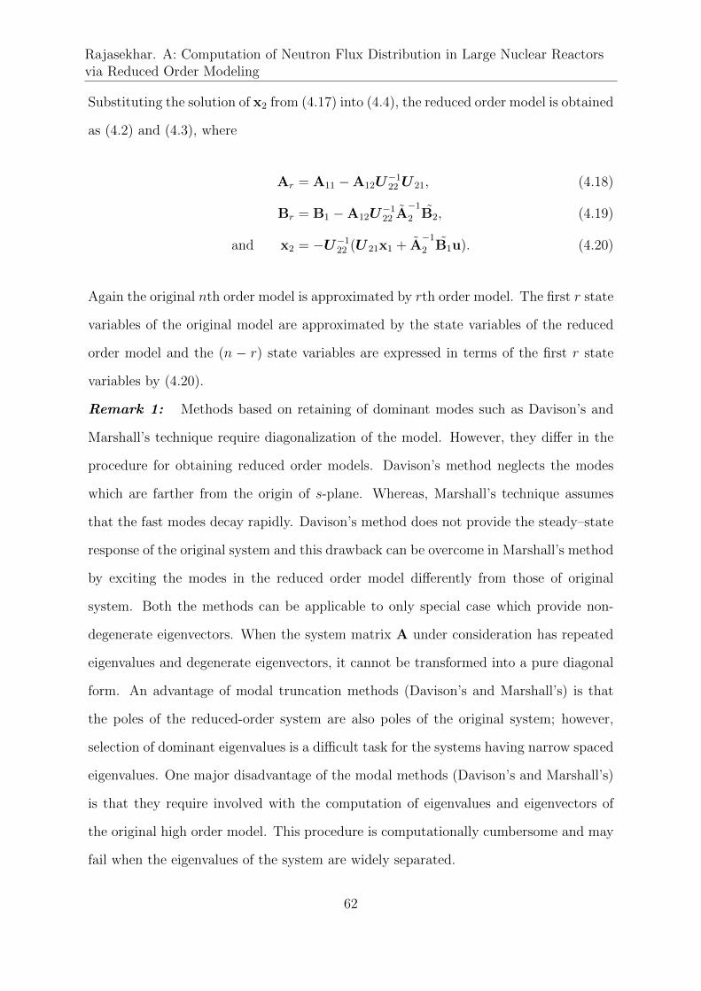
Rajasekhar. A: Computation of Neutron Flux Distribution in Large Nuclear Reactorsvia Reduced Order Modeling
Substituting the solution of x2 from (4.17) into (4.4), the reduced order model is obtained
as (4.2) and (4.3), where
Ar = A11 −A12U−122U 21, (4.18)
Br = B1 −A12U−122 A
−12 B2, (4.19)
and x2 = −U−122 (U 21x1 + A−12 B1u). (4.20)
Again the original nth order model is approximated by rth order model. The first r state
variables of the original model are approximated by the state variables of the reduced
order model and the (n − r) state variables are expressed in terms of the first r state
variables by (4.20).
Remark 1: Methods based on retaining of dominant modes such as Davison’s and
Marshall’s technique require diagonalization of the model. However, they differ in the
procedure for obtaining reduced order models. Davison’s method neglects the modes
which are farther from the origin of s-plane. Whereas, Marshall’s technique assumes
that the fast modes decay rapidly. Davison’s method does not provide the steady–state
response of the original system and this drawback can be overcome in Marshall’s method
by exciting the modes in the reduced order model differently from those of original
system. Both the methods can be applicable to only special case which provide non-
degenerate eigenvectors. When the system matrix A under consideration has repeated
eigenvalues and degenerate eigenvectors, it cannot be transformed into a pure diagonal
form. An advantage of modal truncation methods (Davison’s and Marshall’s) is that
the poles of the reduced-order system are also poles of the original system; however,
selection of dominant eigenvalues is a difficult task for the systems having narrow spaced
eigenvalues. One major disadvantage of the modal methods (Davison’s and Marshall’s)
is that they require involved with the computation of eigenvalues and eigenvectors of
the original high order model. This procedure is computationally cumbersome and may
fail when the eigenvalues of the system are widely separated.
62

Chapter 4. Theory of Model Reduction Techniques
4.4 Singular Perturbation Analysis
In Linear time invariant models of large–scale systems, the interaction of slow and fast
modes is common a feature and it leads the mathematical models to be ill-conditioned
in control design. Singular perturbation analysis [60] provides a simple means to obtain
approximate solutions to the original system as well as it alleviates the high dimen-
sionality problem. This method is based on the assumption that the system can be
separated into two subsystems: fast and slow. Singular perturbation method provides
reduced order model, first by ignoring the fast modes of the system, then improves its
quality of the approximation by reintroducing their effect as ‘boundary layer’ corrections
calculated in separate time–scales.
In this method both the slow and fast modes are retained, but analysis and design
problems are solved in two stages. By a suitable regrouping of the state variables, the
original higher order system can be expressed into standard singularly perturbed form
in which the derivatives of some of the states are multiplied by a small positive scalar
ε, i.e.,
x1 = A11x1 + A12x2 + B1u, x1(0) = x10, (4.21)
εx2 = A21x1 + A22x2 + B2u, x2(0) = x20 (4.22)
and y = Ψ 1x1 + Ψ 2x2. (4.23)
where the n1 dimensional state vector x1 is predominantly slow and the n2 dimensional
state vector x2 contains fast transients superimposed on a slowly varying “quasi–steady–
state”, i.e., ‖x2‖ >> ‖x1‖. The order of the system represented by (4.21) and (4.22)
is n1 + n2. u is the m dimensional input vector and y is the p dimensional output
vector. The scaling parameter ε > 0 represents the speed ratio of the slow versus fast
phenomena. Let µ(A) = {µ1, µ2, . . . , µn} be the set of eigenvalues of system (4.21)–
(4.23). An important characteristic of the system described by (4.21)–(4.23) is that
63
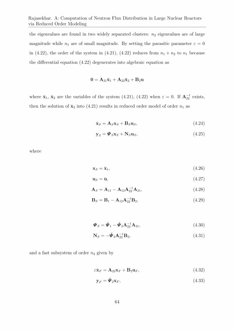
Rajasekhar. A: Computation of Neutron Flux Distribution in Large Nuclear Reactorsvia Reduced Order Modeling
the eigenvalues are found in two widely separated clusters: n2 eigenvalues are of large
magnitude while n1 are of small magnitude. By setting the parasitic parameter ε = 0
in (4.22), the order of the system in (4.21), (4.22) reduces from n1 + n2 to n1 because
the differential equation (4.22) degenerates into algebraic equation as
0 = A21x1 + A22x2 + B2u
where x1, x2 are the variables of the system (4.21), (4.22) when ε = 0. If A−122 exists,
then the solution of x2 into (4.21) results in reduced order model of order n1 as
xS = ASxS + BSuS, (4.24)
yS = ΨSxS + NSuS, (4.25)
where
xS = x1, (4.26)
uS = u, (4.27)
AS = A11 −A12A−122 A21, (4.28)
BS = B1 −A12A−122 B2, (4.29)
ΨS = Ψ 1 − Ψ 2A−122 A21, (4.30)
NS = −Ψ 2A−122 B2, (4.31)
and a fast subsystem of order n2 given by
εxF = A22xF + B2uF , (4.32)
yF = Ψ 2xF , (4.33)
64
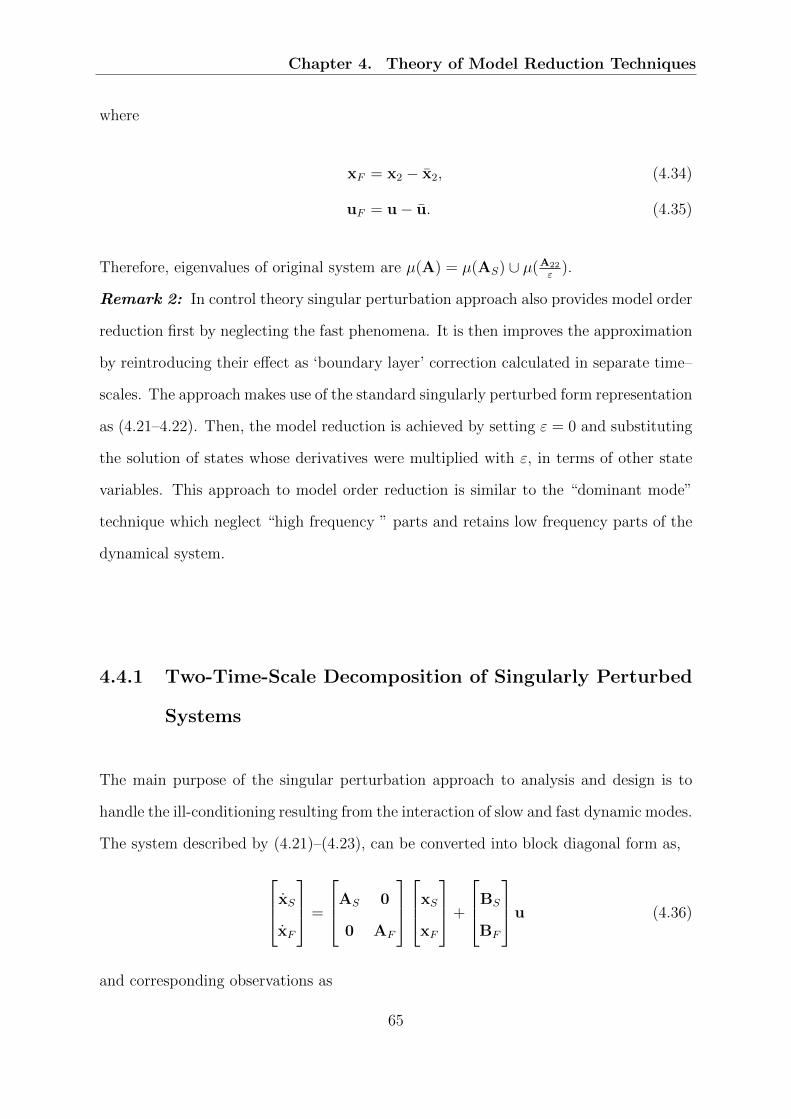
Chapter 4. Theory of Model Reduction Techniques
where
xF = x2 − x2, (4.34)
uF = u− u. (4.35)
Therefore, eigenvalues of original system are µ(A) = µ(AS) ∪ µ(A22
ε).
Remark 2: In control theory singular perturbation approach also provides model order
reduction first by neglecting the fast phenomena. It is then improves the approximation
by reintroducing their effect as ‘boundary layer’ correction calculated in separate time–
scales. The approach makes use of the standard singularly perturbed form representation
as (4.21–4.22). Then, the model reduction is achieved by setting ε = 0 and substituting
the solution of states whose derivatives were multiplied with ε, in terms of other state
variables. This approach to model order reduction is similar to the “dominant mode”
technique which neglect “high frequency ” parts and retains low frequency parts of the
dynamical system.
4.4.1 Two-Time-Scale Decomposition of Singularly Perturbed
Systems
The main purpose of the singular perturbation approach to analysis and design is to
handle the ill-conditioning resulting from the interaction of slow and fast dynamic modes.
The system described by (4.21)–(4.23), can be converted into block diagonal form as,
xS
xF
=
AS 0
0 AF
xS
xF
+
BS
BF
u (4.36)
and corresponding observations as
65

Rajasekhar. A: Computation of Neutron Flux Distribution in Large Nuclear Reactorsvia Reduced Order Modeling
y =
[ΨS ΨF
]xS
xF
, (4.37)
such that µ(A) = µ(AS)∪µ(AF ), where µ(A) denotes the set of eigenvalues of A. The
similarity transformation that is applied to the system given by (4.21)–(4.23) to obtain
the system given by (4.36)–(4.37), is
xS
xF
=
In1 − εML −εM
L In2
x1
x2
, (4.38)
in which In1 and In2 respectively denote n1 and n2 dimensional identity matrices, and
L and M respectively satisfy,
εL = A22L−A21 − εL(A11 −A12L) (4.39)
and εM = −M(A22 + εLA12) + A12 + ε(A11 −A12L)M. (4.40)
L in (4.39) and M in (4.40) can be determined respectively by iterative solution of [63]
Lk+1 = A−122 A21 + εA−122 Lk(A11 −A12Lk), (4.41)
Mk+1 = ε[(A11 −A12Lk)Mk −MkLkA12]A−122
+ A12A−122 ,
(4.42)
L0 = A−122 A21, M0 = A12A−122 , k = 0, 1, 2, ... (4.43)
66
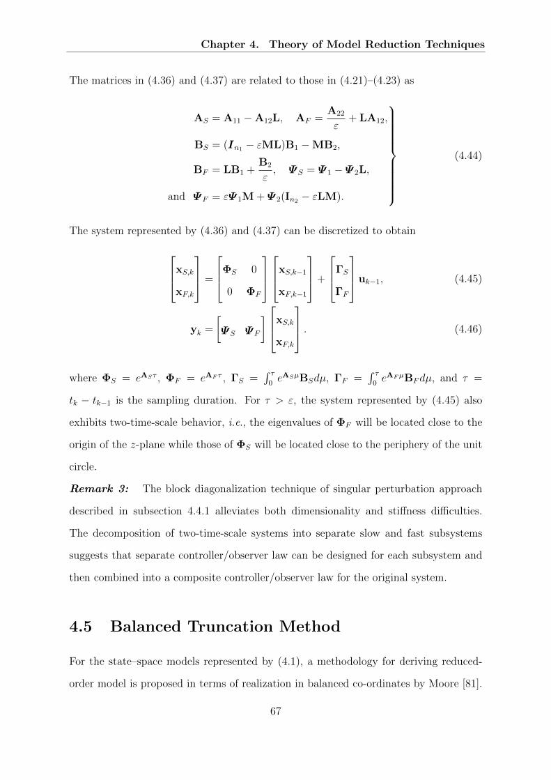
Chapter 4. Theory of Model Reduction Techniques
The matrices in (4.36) and (4.37) are related to those in (4.21)–(4.23) as
AS = A11 −A12L, AF =A22
ε+ LA12,
BS = (In1 − εML)B1 −MB2,
BF = LB1 +B2
ε, ΨS = Ψ 1 − Ψ 2L,
and ΨF = εΨ 1M + Ψ 2(In2 − εLM).
(4.44)
The system represented by (4.36) and (4.37) can be discretized to obtain
xS,k
xF,k
=
ΦS 0
0 ΦF
xS,k−1
xF,k−1
+
ΓS
ΓF
uk−1, (4.45)
yk =
[ΨS ΨF
]xS,k
xF,k
. (4.46)
where ΦS = eASτ , ΦF = eAF τ , ΓS =∫ τ0eASµBSdµ, ΓF =
∫ τ0eAFµBFdµ, and τ =
tk − tk−1 is the sampling duration. For τ > ε, the system represented by (4.45) also
exhibits two-time-scale behavior, i.e., the eigenvalues of ΦF will be located close to the
origin of the z-plane while those of ΦS will be located close to the periphery of the unit
circle.
Remark 3: The block diagonalization technique of singular perturbation approach
described in subsection 4.4.1 alleviates both dimensionality and stiffness difficulties.
The decomposition of two-time-scale systems into separate slow and fast subsystems
suggests that separate controller/observer law can be designed for each subsystem and
then combined into a composite controller/observer law for the original system.
4.5 Balanced Truncation Method
For the state–space models represented by (4.1), a methodology for deriving reduced-
order model is proposed in terms of realization in balanced co-ordinates by Moore [81].
67
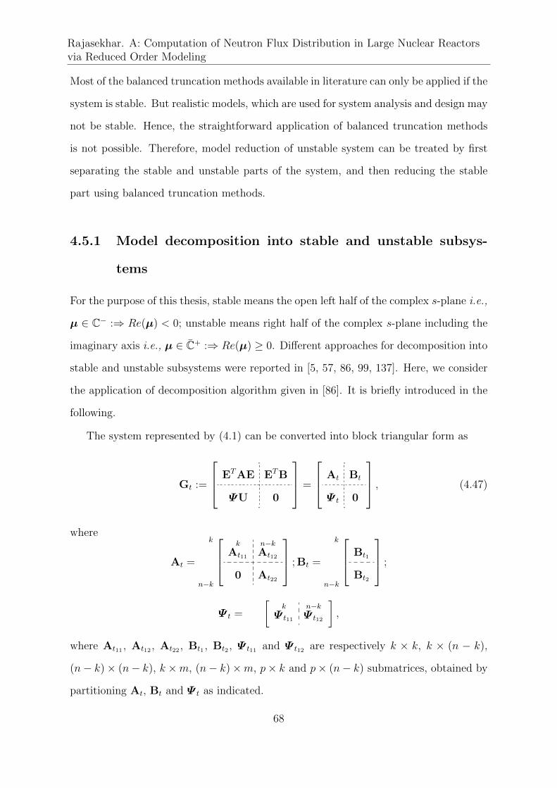
Rajasekhar. A: Computation of Neutron Flux Distribution in Large Nuclear Reactorsvia Reduced Order Modeling
Most of the balanced truncation methods available in literature can only be applied if the
system is stable. But realistic models, which are used for system analysis and design may
not be stable. Hence, the straightforward application of balanced truncation methods
is not possible. Therefore, model reduction of unstable system can be treated by first
separating the stable and unstable parts of the system, and then reducing the stable
part using balanced truncation methods.
4.5.1 Model decomposition into stable and unstable subsys-
tems
For the purpose of this thesis, stable means the open left half of the complex s-plane i.e.,
µ ∈ C− :⇒ Re(µ) < 0; unstable means right half of the complex s-plane including the
imaginary axis i.e., µ ∈ C+ :⇒ Re(µ) ≥ 0. Different approaches for decomposition into
stable and unstable subsystems were reported in [5, 57, 86, 99, 137]. Here, we consider
the application of decomposition algorithm given in [86]. It is briefly introduced in the
following.
The system represented by (4.1) can be converted into block triangular form as
Gt :=
ETAE ETB
ΨU 0
=
At Bt
Ψ t 0
, (4.47)
where
At =
k
n−k
k
At11
n−kAt12
0 At22
; Bt =
k
n−k
Bt1
Bt2
;
Ψ t =
[k
Ψ t11
n−kΨ t12
],
where At11 , At12 , At22 , Bt1 , Bt2 , Ψ t11 and Ψ t12 are respectively k × k, k × (n − k),
(n− k)× (n− k), k ×m, (n− k)×m, p× k and p× (n− k) submatrices, obtained by
partitioning At, Bt and Ψ t as indicated.
68
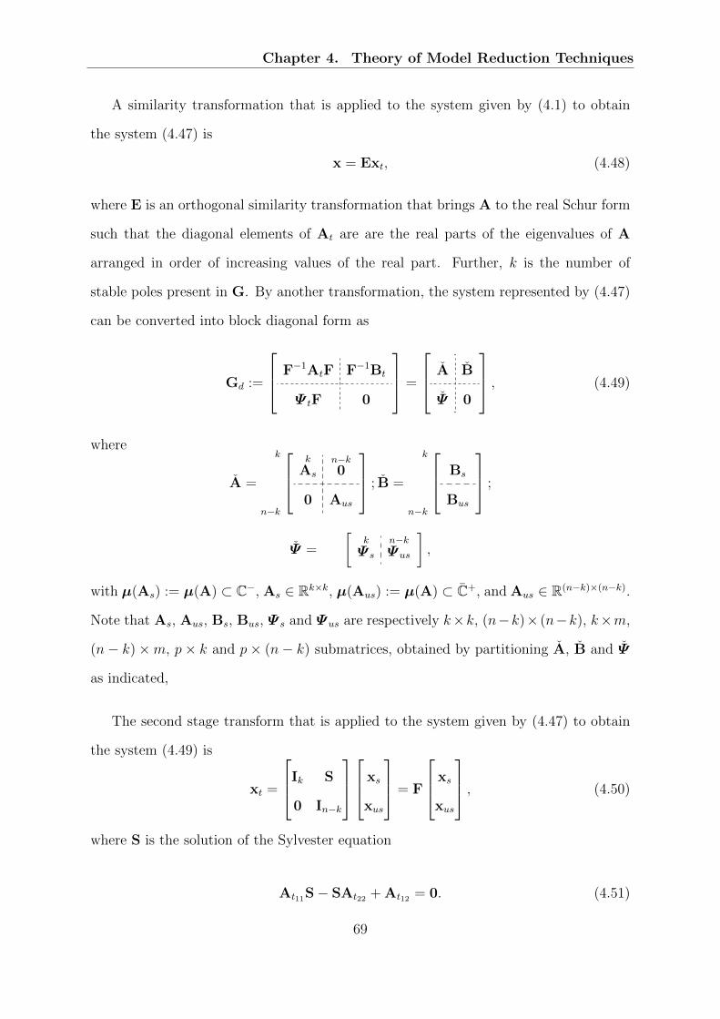
Chapter 4. Theory of Model Reduction Techniques
A similarity transformation that is applied to the system given by (4.1) to obtain
the system (4.47) is
x = Ext, (4.48)
where E is an orthogonal similarity transformation that brings A to the real Schur form
such that the diagonal elements of At are are the real parts of the eigenvalues of A
arranged in order of increasing values of the real part. Further, k is the number of
stable poles present in G. By another transformation, the system represented by (4.47)
can be converted into block diagonal form as
Gd :=
F−1AtF F−1Bt
Ψ tF 0
=
A B
Ψ 0
, (4.49)
where
A =
k
n−k
k
As
n−k0
0 Aus
; B =
k
n−k
Bs
Bus
;
Ψ =
[k
Ψ s
n−kΨus
],
with µ(As) := µ(A) ⊂ C−, As ∈ Rk×k, µ(Aus) := µ(A) ⊂ C+, and Aus ∈ R(n−k)×(n−k).
Note that As, Aus, Bs, Bus, Ψ s and Ψus are respectively k×k, (n−k)× (n−k), k×m,
(n− k)×m, p× k and p× (n− k) submatrices, obtained by partitioning A, B and Ψ
as indicated,
The second stage transform that is applied to the system given by (4.47) to obtain
the system (4.49) is
xt =
Ik S
0 In−k
xs
xus
= F
xs
xus
, (4.50)
where S is the solution of the Sylvester equation
At11S− SAt22 + At12 = 0. (4.51)
69
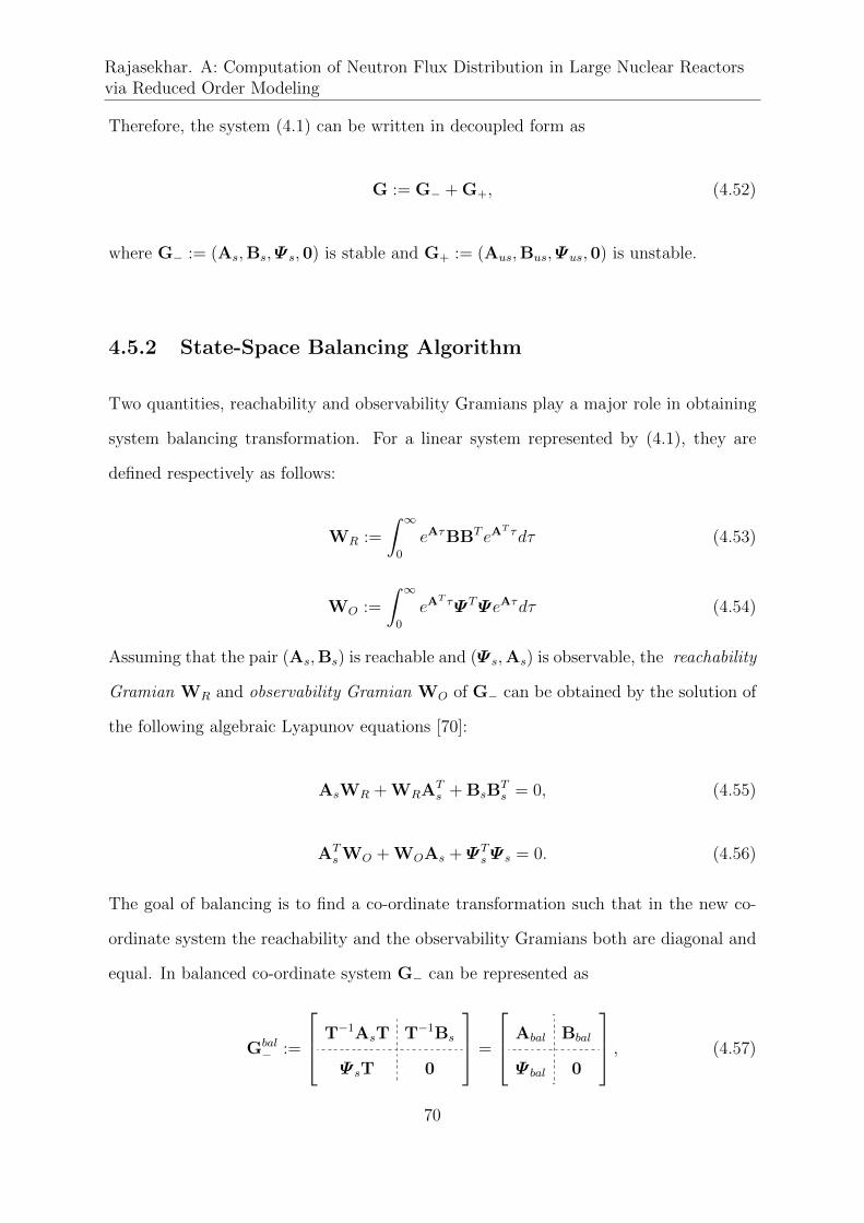
Rajasekhar. A: Computation of Neutron Flux Distribution in Large Nuclear Reactorsvia Reduced Order Modeling
Therefore, the system (4.1) can be written in decoupled form as
G := G− + G+, (4.52)
where G− := (As,Bs,Ψ s,0) is stable and G+ := (Aus,Bus,Ψus,0) is unstable.
4.5.2 State-Space Balancing Algorithm
Two quantities, reachability and observability Gramians play a major role in obtaining
system balancing transformation. For a linear system represented by (4.1), they are
defined respectively as follows:
WR :=
∫ ∞0
eAτBBT eAT τdτ (4.53)
WO :=
∫ ∞0
eAT τΨTΨeAτdτ (4.54)
Assuming that the pair (As,Bs) is reachable and (Ψ s,As) is observable, the reachability
Gramian WR and observability Gramian WO of G− can be obtained by the solution of
the following algebraic Lyapunov equations [70]:
AsWR + WRATs + BsB
Ts = 0, (4.55)
ATs WO + WOAs + ΨT
s Ψ s = 0. (4.56)
The goal of balancing is to find a co-ordinate transformation such that in the new co-
ordinate system the reachability and the observability Gramians both are diagonal and
equal. In balanced co-ordinate system G− can be represented as
Gbal− :=
T−1AsT T−1Bs
Ψ sT 0
=
Abal Bbal
Ψ bal 0
, (4.57)
70
Chapter 4. Theory of Model Reduction Techniques
where
Abal =
r
k−r
r
A(11)bal
k−r
A(12)bal
A(21)bal A
(22)bal
; Bbal =
r
k−r
B(1)bal
B(2)bal
;
Ψ bal =
[r
Ψ(1)bal
k−r
Ψ(2)bal
],
where A(11)bal , A
(12)bal , A
(21)bal , A
(22)bal , B
(1)bal, B
(2)bal, Ψ
(1)bal and Ψ
(2)bal are respectively r×r, r×(k−r),
(k − r) × r, (k − r) × (k − r), r ×m, (r − k) ×m, p × r and p × (k − r) submatrices,
obtained by partitioning Abal, Bbal and Ψ bal as indicated. Further, r is the number of
states which are to be retained in Gbal− . The procedure for obtaining Gbal
− and selection
of r are discussed in the following.
A similarity transformation to obtain Gbal− from G− is
xs = Txsb , (4.58)
where T ∈ Rk×k is nonsingular. Following [70], an algorithm for computation of balanc-
ing transformation is as follows:
(1) Compute the Gramians WR and WO for G−.
(2) Compute the Cholesky factors of WR and WO i.e., WR = LRLTR, WO = LOL
TO,
where LR and LO denote lower triangular Cholesky factors.
(3) Compute SVD of product of Cholesky factors, i.e., LTOLR = UΣVT
(4) Finally, a co-ordinate transformation that results in balanced realization can be
obtained as
T = LRVΣ−1/2. (4.59)
Gbal− is asymptotically stable and is in balanced realization form with
WR = WO = diag.
[Σ1 Σ2
], (4.60)
71
Rajasekhar. A: Computation of Neutron Flux Distribution in Large Nuclear Reactorsvia Reduced Order Modeling
where
Σ1 = diag. [σ1 σ2 . . . σr], Σ2 = diag. [σr+1 σr+2 . . . σk],
σr > σr+1 and σi > 0, i = 1, 2, . . . , k, σi are the Hankel singular values of Gbal− . One
usually tries to choose r so that we have σr � σr+1, in addition to other criteria like
desired accuracy and sought order of the reduced order model. Therefore, the system
(4.1) can be represented in additive TF form as
G(s) := G+(s) + Gbal− (s), (4.61)
where Gbal− := (Abal,Bbal,Ψ bal,0) is balanced and stable. Let
x1
x2
x3
=
η11 η12 η13
η21 η22 η23
η31 η32 η33
xus
xsb1
xsb2
(4.62)
where xus ∈ Rn−k, xsb1 ∈ Rr, and xsb2 ∈ Rk−r be a similarity transformation to obtain
(4.61) from (4.1). Hankel singular values for the system are defined as the square roots
of the eigenvalues of the product WRWO. The balanced basis has the property that
the states which are difficult to reach are simultaneously difficult to observe. The states
in Gbal− corresponding to the largest singular values are most important in the input-
output behavior. Truncation of the states corresponding to the smaller Hankel singular
values i.e., Σ2 will result in a reduced order model Gr whose input-output behavior
closely approximates the behavior of the original model. More precisely, the H∞ norm
of the difference between full-order system G and the reduced order system Gr is upper
bounded by twice the sum of the neglected Hankel singular values [2] and given as
‖G− Gr‖H∞ 6 2(σr+1 + · · ·+ σk). (4.63)
72

Chapter 4. Theory of Model Reduction Techniques
Therefore, a reduced order model for the system (4.1) can be obtained as
Gr :=
Ar Br
Ψ r 0
, (4.64)
where
Ar =
n−k
r
n−kAus
r
0
0 A(11)bal
; Br =
n−k
r
Bus
B(1)bal
;
Ψ r =
[n−kΨus
r
Ψ(1)bal
].
Reduced order model of (4.1) in terms of original co-ordinate system can be obtained
by setting xsb2 = 0 in (4.62) as
˙x = ΛArΛ−1x +ΛBru, (4.65)
y = Ψ rΛ−1x, (4.66)
where x =
x1
x2
, Λ =
η11 η12
η21 η22
. Moreover, from (4.62) we have
x3 = ξ
x1
x2
, where ξ =
[η31 η32
]Λ−1. (4.67)
Thus, the original n th order model represented by (4.1) is reduced to (n − k + r) th
order model. The state variables of the reduced order model are defined as the first
(n− k+ r) state variables of the original model. Though we do not need the remaining
(k− r) state variables of original model, if they are required in an application, they can
be expressed in terms of the first (n− k + r) state variables by using (4.67).
Remark 4: : Model reduction by balanced truncation requires balancing the whole
system G− followed by truncation. The Lyapunov equations (4.55) and (4.56) play a
73
Rajasekhar. A: Computation of Neutron Flux Distribution in Large Nuclear Reactorsvia Reduced Order Modeling
prominent role in obtaining system balancing transformation T and are required to be
solved to obtain WR and WO. The Bartels-Stewart and Hammarling methods are di-
rect standard methods for the solution of Lyapunov equations of small to moderate size.
These methods rely on initial Schur decomposition of As followed by additional factor-
ization schemes. In general and especially for large-scale systems, it is unwise to solve for
WR and WO directly since these require arithmetic operations of order N3 represent-
ing computational complexity and storage of order N2, where N is the original system
order. This approach may turn out to be numerically inefficient and ill-conditioned as
the Gramians WR and WO often have numerically low rank i.e., the eigenvalues of WR
and WO decay rapidly. However, results on low rank approximations to the solutions
of Lyapunov equations based on iterative methods (SVD-Krylov methods) make the
balanced truncation model reduction approach feasible for large-scale systems [2, 4, 93].
74
Chapter 5
Application of Model Order
Reduction Techniques to
Space–Time Kinetics Model of
AHWR
In chapter-3, the dynamical model describing the time–dependent core neutronics
behavior of the AHWR has been derived. This complex nonlinear mathematical model
(core neutronics and control rod dynamic equations) can be linearized around steady–
state operating point to obtain a linear model for the purpose of estimation. An im-
portant characteristic of this nodal method based model, is that the order depends
on the number of nodes into which the reactor spatial domain is divided. A rigorous
model with more number of nodes will give good accuracy in online monitoring and
control, but its order is also very high. At the same time, nuclear reactor models often
exhibit simultaneous presence of dynamics of different speeds. Such behavior leads to
Parts of this chapter were published in 2015 IEEE international Conference on Industrial Instru-mentation and Control Applications (ICIC), Pune, India and in Annals of Nuclear Energy, Vol. 102.
75
Rajasekhar. A: Computation of Neutron Flux Distribution in Large Nuclear Reactorsvia Reduced Order Modeling
a mathematical model with multiple time-scales, which may be susceptible to numer-
ical ill-conditioning in flux mapping studies. Hence, there is a strong motivation for
obtaining a suitable reduced order model which alleviates the high dimensionality and
numerical ill-conditioning problems in computations.
This chapter presents the derivation of an estimation model for flux distribution
studies in the AHWR and also the comparative study between different reduced order
models of AHWR, namely, Davison’s technique, Marshall’s technique, singular pertur-
bation analysis and balanced truncation, by comparing their performances relative to
each other and with the original model.
5.1 Derivation of Estimation Model
The system of nonlinear equations (3.18)–(3.22) is linearized around the steady–state
operating point (φh0, Ch0, Hj0), by considering a small perturbation in neutron flux
level, delayed neutron precursor concentration (for simplicity, only one group of delayed
neutron precursors is considered instead of six groups), RR position and the input volt-
ages to RR drives, denoted respectively by δφh, δCh, δHh and δϑl around the operating
point. Now from (3.18)–(3.20) and (3.22), we have
d
dt
(δφhφh0
)=[− ωhhυh +
ρh0`h− β
`h
]δφhφh0
+
Nh∑k=1
ωhkυh
(φk0φh0
)δφkφk0
(5.1)
+β
`h
δChCh0− 10.234× 10⁻⁶ × φh0
`hδHh,
h = 1, 2, 3, ..., Zp,
d
dt
(δChCh0
)= λ
δφhφh0− λδCh
Ch0, h = 1, 2, 3, . . . , Zp (5.2)
d
dt
(δφhφh0
)=− ωhhυh
δφhφh0
+
Nh∑k=1
ωhkυh
(φk0φh0
)δφkφk0
, (5.3)
h = Zp + 1, . . . , Zp + Zr,
76

Chapter 5. Application of Model Order Reduction Techniques toSpace–Time Kinetics Model of AHWR
dδHl
dt= KRRδϑl, l = 2, 4, 6, 8. (5.4)
where δ denotes the deviation from respective steady–state values. In (5.1), the term
δHl denoting the deviation in position of the lth RR from that corresponding to the
critical configuration, will be present only if the node h contains the RR-l. Now, let us
define the state vector as
x :=
[xTφC xTC xTφR xTH
]T(5.5)
where
xφC :=
[δφ1/φ10 ... δφ17/φ170
]T, (5.6)
xC :=
[δC1/C10 ... δC17/φ170
]T, (5.7)
xφR :=
[δφ18/φ180 ... δφ59/φ590
]T, (5.8)
xH :=
[δH2 δH4 δH6 δH8
]T. (5.9)
In (5.5), xφC and xC denote the state vectors corresponding to the deviation in nor-
malized neutron flux and associated deviation in precursors’ concentration in the core
nodes respectively. xφR denotes state vector corresponding to the deviation in normal-
ized neutron flux in reflector nodes, xH denotes the state vector corresponding to the
deviation in the position of RRs.
Also, define the input vector as
u =
[δϑ2 δϑ4 δϑ6 δϑ8
]T. (5.10)
As already introduced, δϑl denotes deviation of applied to lth RR. Then, the system
of equations (5.1)–(5.4) which constitute the estimation model can be represented in
standard linear state–space form of (4.1). The system matrix A of size 80 × 80, is
77
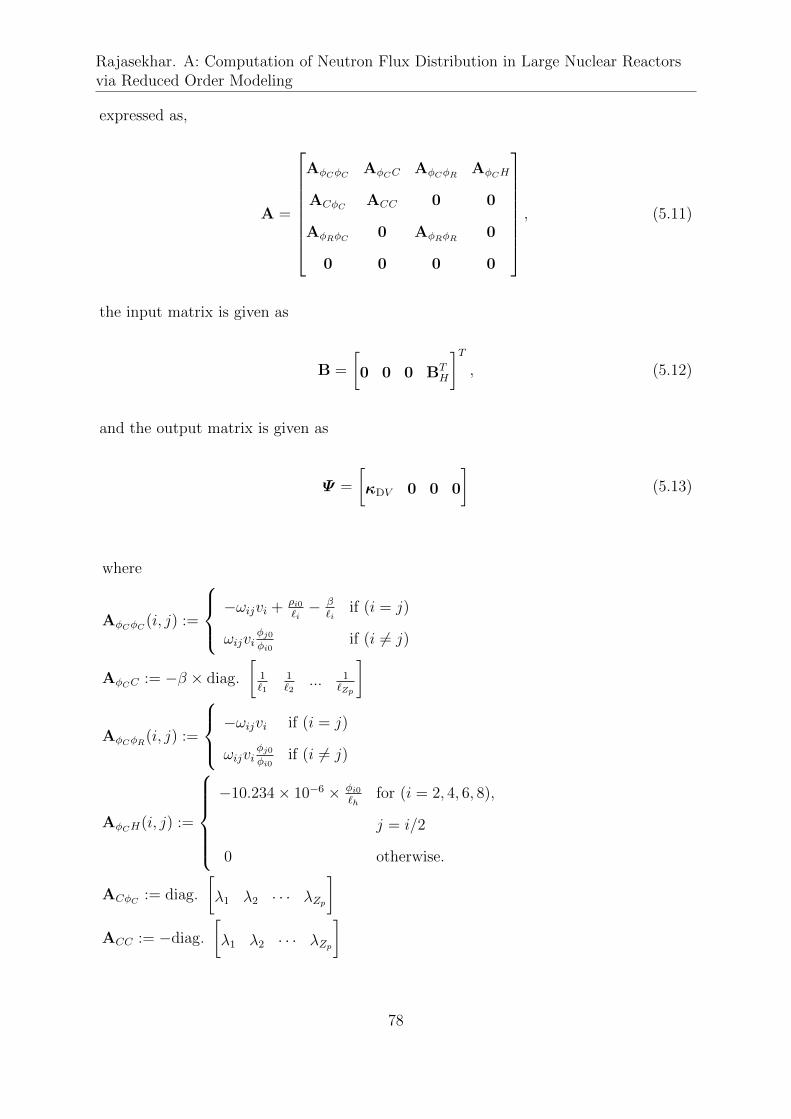
Rajasekhar. A: Computation of Neutron Flux Distribution in Large Nuclear Reactorsvia Reduced Order Modeling
expressed as,
A =
AφCφC AφCC AφCφR AφCH
ACφC ACC 0 0
AφRφC 0 AφRφR 0
0 0 0 0
, (5.11)
the input matrix is given as
B =
[0 0 0 BT
H
]T, (5.12)
and the output matrix is given as
Ψ =
[κDV 0 0 0
](5.13)
where
AφCφC (i, j) :=
−ωijvi + ρi0`i− β
`iif (i = j)
ωijviφj0φi0
if (i 6= j)
AφCC := −β × diag.
[1`1
1`2
... 1`Zp
]
AφCφR(i, j) :=
−ωijvi if (i = j)
ωijviφj0φi0
if (i 6= j)
AφCH(i, j) :=
−10.234× 10⁻⁶ × φi0
`hfor (i = 2, 4, 6, 8),
j = i/2
0 otherwise.
ACφC := diag.
[λ1 λ2 · · · λZp
]ACC := −diag.
[λ1 λ2 · · · λZp
]
78
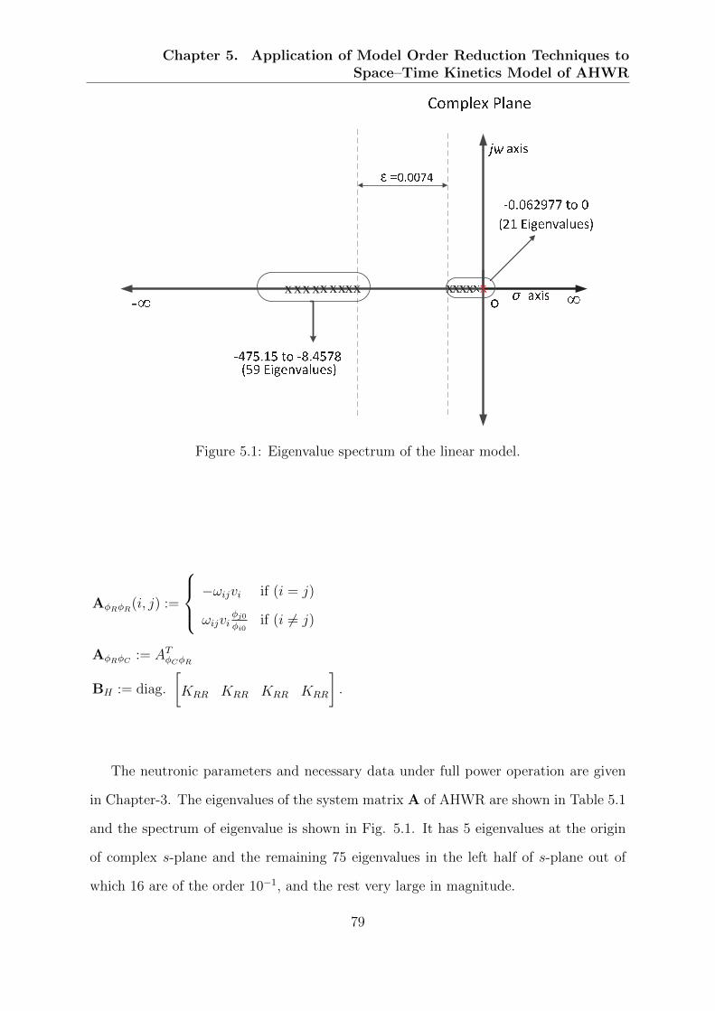
Chapter 5. Application of Model Order Reduction Techniques toSpace–Time Kinetics Model of AHWR
xxxxxxxxxxx x xx
�
Figure 5.1: Eigenvalue spectrum of the linear model.
AφRφR(i, j) :=
−ωijvi if (i = j)
ωijviφj0φi0
if (i 6= j)
AφRφC := ATφCφR
BH := diag.
[KRR KRR KRR KRR
].
The neutronic parameters and necessary data under full power operation are given
in Chapter-3. The eigenvalues of the system matrix A of AHWR are shown in Table 5.1
and the spectrum of eigenvalue is shown in Fig. 5.1. It has 5 eigenvalues at the origin
of complex s-plane and the remaining 75 eigenvalues in the left half of s-plane out of
which 16 are of the order 10−1, and the rest very large in magnitude.
79
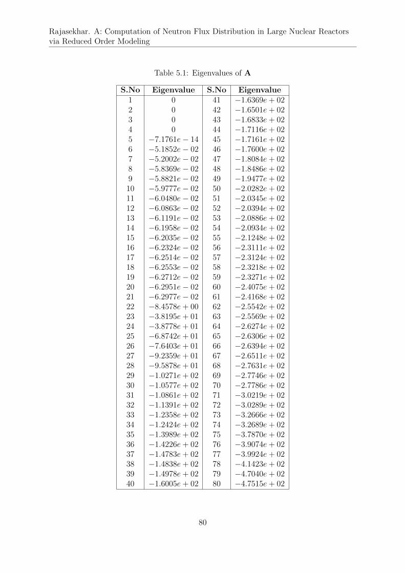
Rajasekhar. A: Computation of Neutron Flux Distribution in Large Nuclear Reactorsvia Reduced Order Modeling
Table 5.1: Eigenvalues of A
S.No Eigenvalue S.No Eigenvalue1 0 41 −1.6369e+ 022 0 42 −1.6501e+ 023 0 43 −1.6833e+ 024 0 44 −1.7116e+ 025 −7.1761e− 14 45 −1.7161e+ 026 −5.1852e− 02 46 −1.7600e+ 027 −5.2002e− 02 47 −1.8084e+ 028 −5.8369e− 02 48 −1.8486e+ 029 −5.8821e− 02 49 −1.9477e+ 0210 −5.9777e− 02 50 −2.0282e+ 0211 −6.0480e− 02 51 −2.0345e+ 0212 −6.0863e− 02 52 −2.0394e+ 0213 −6.1191e− 02 53 −2.0886e+ 0214 −6.1958e− 02 54 −2.0934e+ 0215 −6.2035e− 02 55 −2.1248e+ 0216 −6.2324e− 02 56 −2.3111e+ 0217 −6.2514e− 02 57 −2.3124e+ 0218 −6.2553e− 02 58 −2.3218e+ 0219 −6.2712e− 02 59 −2.3271e+ 0220 −6.2951e− 02 60 −2.4075e+ 0221 −6.2977e− 02 61 −2.4168e+ 0222 −8.4578e+ 00 62 −2.5542e+ 0223 −3.8195e+ 01 63 −2.5569e+ 0224 −3.8778e+ 01 64 −2.6274e+ 0225 −6.8742e+ 01 65 −2.6306e+ 0226 −7.6403e+ 01 66 −2.6394e+ 0227 −9.2359e+ 01 67 −2.6511e+ 0228 −9.5878e+ 01 68 −2.7631e+ 0229 −1.0271e+ 02 69 −2.7746e+ 0230 −1.0577e+ 02 70 −2.7786e+ 0231 −1.0861e+ 02 71 −3.0219e+ 0232 −1.1391e+ 02 72 −3.0289e+ 0233 −1.2358e+ 02 73 −3.2666e+ 0234 −1.2424e+ 02 74 −3.2689e+ 0235 −1.3989e+ 02 75 −3.7870e+ 0236 −1.4226e+ 02 76 −3.9074e+ 0237 −1.4783e+ 02 77 −3.9924e+ 0238 −1.4838e+ 02 78 −4.1423e+ 0239 −1.4978e+ 02 79 −4.7040e+ 0240 −1.6005e+ 02 80 −4.7515e+ 02
80
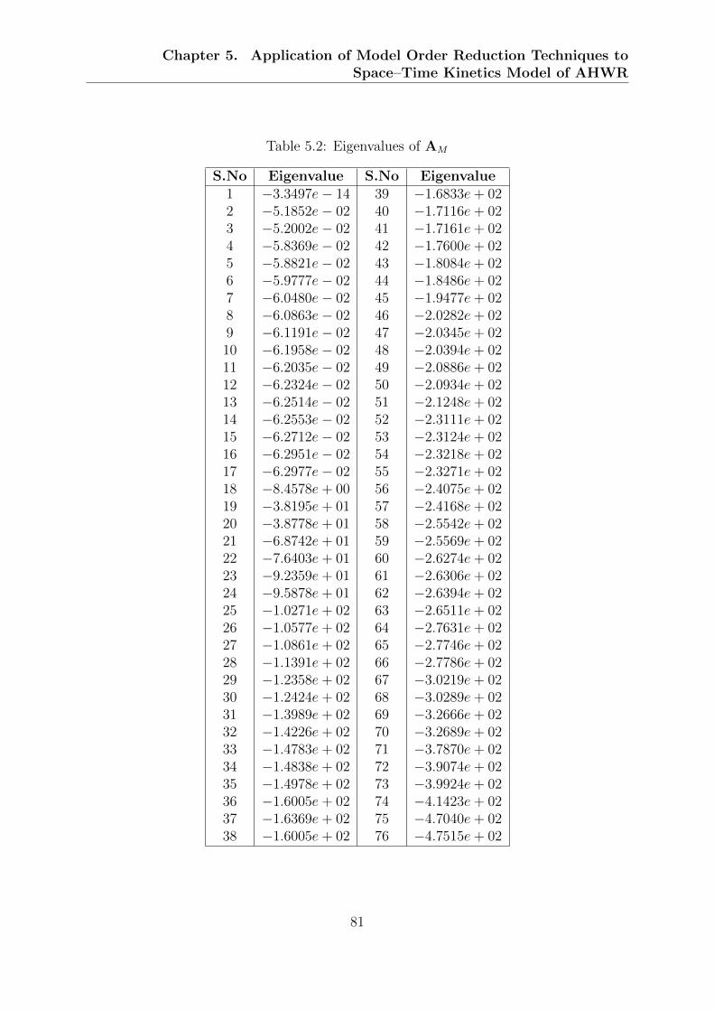
Chapter 5. Application of Model Order Reduction Techniques toSpace–Time Kinetics Model of AHWR
Table 5.2: Eigenvalues of AM
S.No Eigenvalue S.No Eigenvalue1 −3.3497e− 14 39 −1.6833e+ 022 −5.1852e− 02 40 −1.7116e+ 023 −5.2002e− 02 41 −1.7161e+ 024 −5.8369e− 02 42 −1.7600e+ 025 −5.8821e− 02 43 −1.8084e+ 026 −5.9777e− 02 44 −1.8486e+ 027 −6.0480e− 02 45 −1.9477e+ 028 −6.0863e− 02 46 −2.0282e+ 029 −6.1191e− 02 47 −2.0345e+ 0210 −6.1958e− 02 48 −2.0394e+ 0211 −6.2035e− 02 49 −2.0886e+ 0212 −6.2324e− 02 50 −2.0934e+ 0213 −6.2514e− 02 51 −2.1248e+ 0214 −6.2553e− 02 52 −2.3111e+ 0215 −6.2712e− 02 53 −2.3124e+ 0216 −6.2951e− 02 54 −2.3218e+ 0217 −6.2977e− 02 55 −2.3271e+ 0218 −8.4578e+ 00 56 −2.4075e+ 0219 −3.8195e+ 01 57 −2.4168e+ 0220 −3.8778e+ 01 58 −2.5542e+ 0221 −6.8742e+ 01 59 −2.5569e+ 0222 −7.6403e+ 01 60 −2.6274e+ 0223 −9.2359e+ 01 61 −2.6306e+ 0224 −9.5878e+ 01 62 −2.6394e+ 0225 −1.0271e+ 02 63 −2.6511e+ 0226 −1.0577e+ 02 64 −2.7631e+ 0227 −1.0861e+ 02 65 −2.7746e+ 0228 −1.1391e+ 02 66 −2.7786e+ 0229 −1.2358e+ 02 67 −3.0219e+ 0230 −1.2424e+ 02 68 −3.0289e+ 0231 −1.3989e+ 02 69 −3.2666e+ 0232 −1.4226e+ 02 70 −3.2689e+ 0233 −1.4783e+ 02 71 −3.7870e+ 0234 −1.4838e+ 02 72 −3.9074e+ 0235 −1.4978e+ 02 73 −3.9924e+ 0236 −1.6005e+ 02 74 −4.1423e+ 0237 −1.6369e+ 02 75 −4.7040e+ 0238 −1.6005e+ 02 76 −4.7515e+ 02
81
Rajasekhar. A: Computation of Neutron Flux Distribution in Large Nuclear Reactorsvia Reduced Order Modeling
5.2 Model Order Reduction of AHWR Space–Time
Kinetics Model
In this Section, for the estimation model of AHWR derived in the previous Section, var-
ious model order reduction techniques, viz., Davison’s and Marshall’s dominant mode
retention techniques, model decomposition into slow and fast subsystems based on sin-
gular perturbation analysis and balanced truncation technique have been applied to
obtain a reduced order model from the original high order model.
For the study in this section, we define the output vector as y =
[y1 · · · y17
]T,
where yi = δφi/φi0 denotes the corresponding deviation in nodal flux. Therefore, output
matrix is given as
Ψ =
[ΨφC 0 0 0
], (5.14)
and ΨφC := IZp , where IZp denotes an Identity matrix.
From Table 5.1, it is evident that, there are multiple eigenvalues at the origin of
the complex s-plane. Hence, diagonalization of the estimation model is not possible.
However, this difficulty is overcome by rewriting the dynamics of the original system.
State vector (5.5) is regrouped and the dynamics of original system are rewritten such
that the control rod dynamics are decoupled. The decoupled set of equations are:
xM = AMxM + BMxH , (5.15)
y = ΨMxM , (5.16)
and xH = BHu (5.17)
where xM =
[xTC xTφR xTφC
]Tis of order 76 and BM =
[0 0 AT
φCH
]T,
AM =
ACC 0 ACφC
0 AφRφR AφRφC
AφCC AφCφR AφCφC
, (5.18)
82
Chapter 5. Application of Model Order Reduction Techniques toSpace–Time Kinetics Model of AHWR
and
ΨM =
[0 0 ΨφC
]. (5.19)
Eigenvalues of AM are shown in Table 5.2. It can be verified that all the eigenvalues of
AM are distinct. In fact, eigenvalues of AM are approximately equal to the 76 eigenvalues
of A, listed at S.No 5 to 80 in Table 5.1. Now the model reduction techniques discussed
in Section 4.2 and Section 4.3 can be directly applied to the 76th order model, given
by (5.15) and (5.16), for obtaining the simplified models. Finally, by augmenting the
control rod dynamics the simplified model for AHWR can be represented as,
xR =
xr
xH
=
Ar Br
0 0
xr
xH
+
0
BH
u, (5.20)
y =
[Ψ r 0
]xr
xH
. (5.21)
5.2.1 Reduced Model Based on Davison’s Technique
First consider the application of Davison’s technique discussed in Section 4.2 to the
estimation model given by (5.15) and (5.16) so as to retain the 17 eigenvalues of AM ,
listed at S.No 1 to 17 in Table 5.2. However, the reduced order model thus obtained
does not yield satisfactory approximation as deviation between responses of the original
system and simplified model are seem to be large. Therefore, another state δφ1/φ10 has
been included in the reduced order model to achieve the satisfactory transient perfor-
mance with respect to original model. Thus, eigenvalue −8.4578 (S.No. 18) has also
been retained in the simplified model. By substituting the matrices Ar,Br and Ψ r in
(5.20) and (5.21) thus obtained, the following simplified model of order 22 is obtained
for AHWR.
xR = AdxR + Bdu. (5.22)
yd = ΨdxR, (5.23)
83
Rajasekhar. A: Computation of Neutron Flux Distribution in Large Nuclear Reactorsvia Reduced Order Modeling
where xR =
[xTC δφ1/φ10 xTH
]Tis the reduced state vector of order 22 × 1. Ad, Bd
and Ψd are corresponding system, input and output matrices of the AHWR simplified
model obtained by the application of Davison’s technique. The eigenvalues retained in
simplified model are the first 22 eigenvalues of the original system shown in Table 5.1.
5.2.2 Reduced Model Based on Marshall’s Technique
The Marshall’s technique discussed in Section 4.3 can be applied to the estimation model
given by (5.15) and (5.16) so as to retain the 17 eigenvalues of A, listed at S.No 5 to
21 in Table 5.1. By substituting the matrices Ar,Br and Ψr in (5.20) and (5.21) thus
obtained, the following simplified model of order 21 is obtained for AHWR.
xR = AmxR + Bmu, (5.24)
ym = ΨmxR, (5.25)
where xR =
[xTC xTH
]Tis the reduced state vector of order 21 × 1. Am, Bm and Ψm
are corresponding system input and output matrices of the AHWR simplified model ob-
tained by the application of Marshall’s technique. The eigenvalues retained in simplified
model are the first 21 eigenvalues of the original system shown in Table 5.1.
5.2.3 Reduced Model Based on Singular Perturbation Analysis
An observation of the eigenvalues of the system matrix A reveals that the eigenvalues
fall into two distinct clusters. First cluster has 21 eigenvalues consisting of 5 eigenvalues
at the origin and the other 16 eigenvalues ranging from −6.2977 × 10⁻² to −5.1852 ×
10−2 and the second one is of 59 eigenvalues ranging from −4.751 × 10² to −8.4578.
The distance between these two eigenvalue clusters, computed by dividing the largest
absolute value of the slow (first) group by the smallest absolute value of the fast (second)
group, is ε = 0.0074. This indicates the presence of two-time-scales in the estimation
84

Chapter 5. Application of Model Order Reduction Techniques toSpace–Time Kinetics Model of AHWR
model. It would therefore, be possible to decompose the model into a slow subsystem of
order 21 and a fast subsystem of order 59, by the application of the method presented
in Section 4.4. For carrying out this, the following regrouping of states is suggested:
x1 =
[xTH xTC
]T(5.26)
x2 =
[xTφR xTφC
]T(5.27)
The sub matrices A11, A12, A21, A22, B1, B2, Ψ 1 and Ψ 2 in (4.21), (4.22) and (4.23)
are obtained by appropriate rearrangement and partitioning of matrices A, B and Ψ
which are given respectively by (5.11), (5.12) and (5.14). Using these, a slow subsystem
of order 21 with AS, BS, ΨS and NS represented by (4.24) and (4.25) is obtained and
it can be considered as the simplified model of the AHWR.
5.2.4 Reduced Model Based on Balanced Truncation
The balanced truncation technique discussed in Section 4.5 can also be applied to the
AHWR model for obtaining the reduced order model with lesser dimension than the
original. The model has 80 states, 4 inputs and 17 outputs. The presence of the
five eigenvalues at the origin restricts the straightforward application of the state-space
balancing method described in Section 4.5.1. Therefore, we carry out stable and unstable
decomposition of the AHWR model described by (5.11) and (5.12) to obtain an unstable
subsystem of order 5 and a stable subsystem of order 75. Thereafter, we calculate the
similarity transformation T in (4.58) was calculated such that the reachability and
observability Gramians in the transformed co-ordinate system are diagonal and equal.
Corresponding Hankel singular values of G are shown in Table 5.3. Fig. 5.2 shows the
Hankel singular values, which represent the “energy” of each state in the balanced system
of AHWR. Before applying the truncation of the system Gbal− , it is necessary to determine
the partitioning of the Hankel singular values. We consider the first five Hankel singular
85
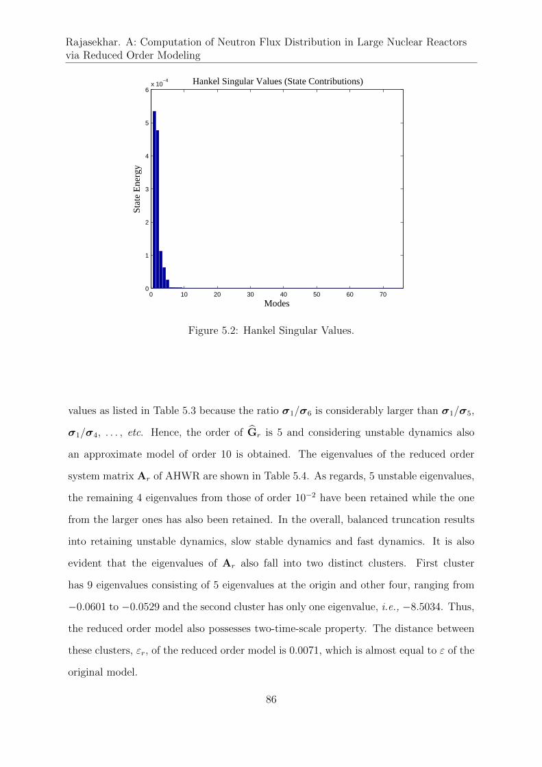
Rajasekhar. A: Computation of Neutron Flux Distribution in Large Nuclear Reactorsvia Reduced Order Modeling
0 10 20 30 40 50 60 700
1
2
3
4
5
6x 10
−4 Hankel Singular Values (State Contributions)
Modes
Stat
e E
nerg
y
Figure 5.2: Hankel Singular Values.
values as listed in Table 5.3 because the ratio σ1/σ6 is considerably larger than σ1/σ5,
σ1/σ4, . . . , etc. Hence, the order of Gr is 5 and considering unstable dynamics also
an approximate model of order 10 is obtained. The eigenvalues of the reduced order
system matrix Ar of AHWR are shown in Table 5.4. As regards, 5 unstable eigenvalues,
the remaining 4 eigenvalues from those of order 10−2 have been retained while the one
from the larger ones has also been retained. In the overall, balanced truncation results
into retaining unstable dynamics, slow stable dynamics and fast dynamics. It is also
evident that the eigenvalues of Ar also fall into two distinct clusters. First cluster
has 9 eigenvalues consisting of 5 eigenvalues at the origin and other four, ranging from
−0.0601 to −0.0529 and the second cluster has only one eigenvalue, i.e., −8.5034. Thus,
the reduced order model also possesses two-time-scale property. The distance between
these clusters, εr, of the reduced order model is 0.0071, which is almost equal to ε of the
original model.
86
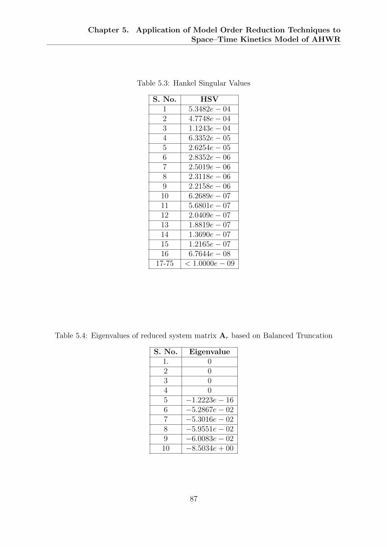
Chapter 5. Application of Model Order Reduction Techniques toSpace–Time Kinetics Model of AHWR
Table 5.3: Hankel Singular Values
S. No. HSV1 5.3482e− 042 4.7748e− 043 1.1243e− 044 6.3352e− 055 2.6254e− 056 2.8352e− 067 2.5019e− 068 2.3118e− 069 2.2158e− 0610 6.2689e− 0711 5.6801e− 0712 2.0409e− 0713 1.8819e− 0714 1.3690e− 0715 1.2165e− 0716 6.7644e− 08
17-75 < 1.0000e− 09
Table 5.4: Eigenvalues of reduced system matrix Ar based on Balanced Truncation
S. No. Eigenvalue1. 02 03 04 05 −1.2223e− 166 −5.2867e− 027 −5.3016e− 028 −5.9551e− 029 −6.0083e− 0210 −8.5034e+ 00
87
Rajasekhar. A: Computation of Neutron Flux Distribution in Large Nuclear Reactorsvia Reduced Order Modeling
5.3 Comparison of Different Reduced Order Mod-
els with the Application of Space-Time Kinetics
Model of AHWR
As already stated, due to the interaction of slow and fast dynamics present in AHWR,
the mathematical model describing its dynamics exhibits the multiple time-scales bring-
ing in susceptibility to numerical ill-conditioning in control design and analysis. In
previous Section, a systematic method has been suggested to handle the numerical ill-
conditioning occurring in the computations due to the presence of the slow control rod
dynamics by decoupling the higher order model into very slow and fast models. Model
order reduction techniques based on Davison’s and Marshall’s dominant mode retention
are then applied to retain the slow dynamics. Finally the reduced order model was
formulated by augmenting the control rod dynamics. Model decomposition into slow
and fast subsystems based on singular perturbation analysis has also been explored by
suggesting regrouping of state variables.
In this section, comparison of the performance characteristics of different reduced
order models of AHWR obtained from Davison’s, Marshall’s, singular perturbation anal-
ysis and balanced truncation methods, relative to each other and with the performance
characteristics of the original higher order model has been presented. To illustrate the
dynamic behavior of different reduced order linear models, the open loop response for
a short–time control relevant transient is presented here. Response obtained by the
simulation of original 80th order model is considered as reference. In simulation, the
reactor was assumed to be initially operating at full power and each RR is at 66.7% in
position. At time t = 0 s, control signal of 1 V is applied to RR drive in node 2 and
maintained for 5 s, under which the RR moved linearly into the reactor core. After a
short interval of 5 s, the control signal is made −1 V and is maintained at this level for
10 s. Then the control voltage is made 1 V for 5 s to bring back the RR to its nominal
88
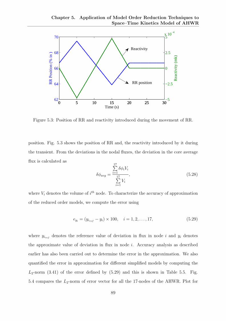
Chapter 5. Application of Model Order Reduction Techniques toSpace–Time Kinetics Model of AHWR
0 5 10 15 20 25 3062
64
66
68
70
RR
Pos
ition
(%
in )
Time (s)0 5 10 15 20 25 30
−5
−2.5
0
2.5
5x 10
−4
Rea
ctiv
ity (
mk)
RR position
Reactivity
Figure 5.3: Position of RR and reactivity introduced during the movement of RR.
position. Fig. 5.3 shows the position of RR and, the reactivity introduced by it during
the transient. From the deviations in the nodal fluxes, the deviation in the core average
flux is calculated as
δφavg =
17∑i=1
δφiVi
17∑i=1
Vi
, (5.28)
where Vi denotes the volume of ith node. To characterize the accuracy of approximation
of the reduced order models, we compute the error using
eyi = (yiref − yi)× 100, i = 1, 2, . . . , 17, (5.29)
where yiref denotes the reference value of deviation in flux in node i and yi denotes
the approximate value of deviation in flux in node i. Accuracy analysis as described
earlier has also been carried out to determine the error in the approximation. We also
quantified the error in approximation for different simplified models by computing the
L2-norm (3.41) of the error defined by (5.29) and this is shown in Table 5.5. Fig.
5.4 compares the L2-norm of error vector for all the 17-nodes of the AHWR. Plot for
89
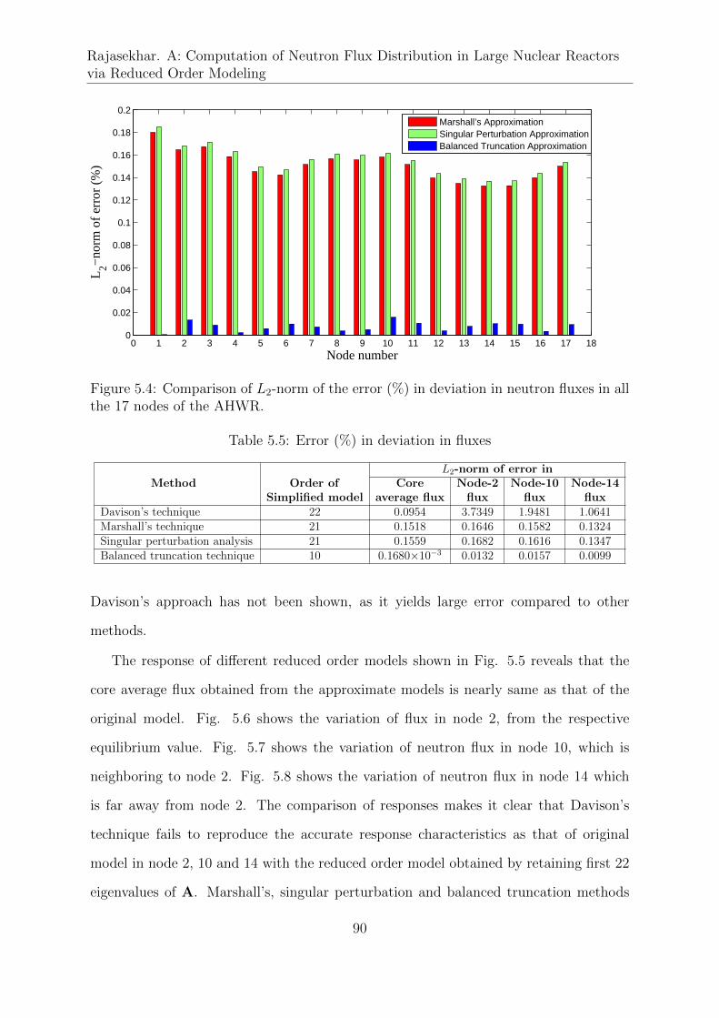
Rajasekhar. A: Computation of Neutron Flux Distribution in Large Nuclear Reactorsvia Reduced Order Modeling
0 1 2 3 4 5 6 7 8 9 10 11 12 13 14 15 16 17 180
0.02
0.04
0.06
0.08
0.1
0.12
0.14
0.16
0.18
0.2
L2−
norm
of e
rror
(%
)
Node number
Marshall’s ApproximationSingular Perturbation ApproximationBalanced Truncation Approximation
Figure 5.4: Comparison of L2-norm of the error (%) in deviation in neutron fluxes in allthe 17 nodes of the AHWR.
Table 5.5: Error (%) in deviation in fluxes
MethodL2-norm of error in
Order of Core Node-2 Node-10 Node-14Simplified model average flux flux flux flux
Davison’s technique 22 0.0954 3.7349 1.9481 1.0641Marshall’s technique 21 0.1518 0.1646 0.1582 0.1324Singular perturbation analysis 21 0.1559 0.1682 0.1616 0.1347Balanced truncation technique 10 0.1680×10⁻³ 0.0132 0.0157 0.0099
Davison’s approach has not been shown, as it yields large error compared to other
methods.
The response of different reduced order models shown in Fig. 5.5 reveals that the
core average flux obtained from the approximate models is nearly same as that of the
original model. Fig. 5.6 shows the variation of flux in node 2, from the respective
equilibrium value. Fig. 5.7 shows the variation of neutron flux in node 10, which is
neighboring to node 2. Fig. 5.8 shows the variation of neutron flux in node 14 which
is far away from node 2. The comparison of responses makes it clear that Davison’s
technique fails to reproduce the accurate response characteristics as that of original
model in node 2, 10 and 14 with the reduced order model obtained by retaining first 22
eigenvalues of A. Marshall’s, singular perturbation and balanced truncation methods
90
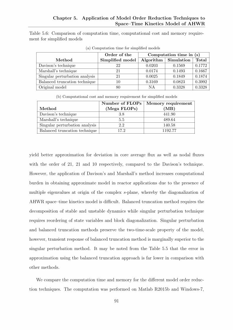
Chapter 5. Application of Model Order Reduction Techniques toSpace–Time Kinetics Model of AHWR
Table 5.6: Comparison of computation time, computational cost and memory require-ment for simplified models
(a) Computation time for simplified models
MethodOrder of the Computation time in (s)
Simplified model Algorithm Simulation Total
Davison’s technique 22 0.0203 0.1569 0.1772
Marshall’s technique 21 0.0174 0.1493 0.1667
Singular perturbation analysis 21 0.0025 0.1849 0.1874
Balanced truncation technique 10 0.3169 0.0823 0.3992
Original model 80 NA 0.3328 0.3328
(b) Computational cost and memory requirement for simplified models
Number of FLOPs Memory requirementMethod (Mega FLOPs) (MB)
Davison’s technique 3.8 441.90
Marshall’s technique 5.5 489.64
Singular perturbation analysis 2.2 140.58
Balanced truncation technique 17.2 1192.77
yield better approximation for deviation in core average flux as well as nodal fluxes
with the order of 21, 21 and 10 respectively, compared to the Davison’s technique.
However, the application of Davison’s and Marshall’s method increases computational
burden in obtaining approximate model in reactor applications due to the presence of
multiple eigenvalues at origin of the complex s-plane, whereby the diagonalization of
AHWR space–time kinetics model is difficult. Balanced truncation method requires the
decomposition of stable and unstable dynamics while singular perturbation technique
requires reordering of state variables and block diagonalization. Singular perturbation
and balanced truncation methods preserve the two-time-scale property of the model,
however, transient response of balanced truncation method is marginally superior to the
singular perturbation method. It may be noted from the Table 5.5 that the error in
approximation using the balanced truncation approach is far lower in comparison with
other methods.
We compare the computation time and memory for the different model order reduc-
tion techniques. The computation was performed on Matlab R2015b and Windows-7,
91
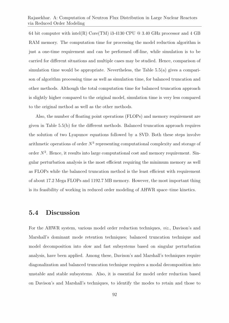
Rajasekhar. A: Computation of Neutron Flux Distribution in Large Nuclear Reactorsvia Reduced Order Modeling
64 bit computer with intel(R) Core(TM) i3-4130 CPU @ 3.40 GHz processor and 4 GB
RAM memory. The computation time for processing the model reduction algorithm is
just a one-time requirement and can be performed off-line, while simulation is to be
carried for different situations and multiple cases may be studied. Hence, comparison of
simulation time would be appropriate. Nevertheless, the Table 5.5(a) gives a compari-
son of algorithm processing time as well as simulation time, for balanced truncation and
other methods. Although the total computation time for balanced truncation approach
is slightly higher compared to the original model, simulation time is very less compared
to the original method as well as the other methods.
Also, the number of floating point operations (FLOPs) and memory requirement are
given in Table 5.5(b) for the different methods. Balanced truncation approach requires
the solution of two Lyapunov equations followed by a SVD. Both these steps involve
arithmetic operations of order N3 representing computational complexity and storage of
order N2. Hence, it results into large computational cost and memory requirement. Sin-
gular perturbation analysis is the most efficient requiring the minimum memory as well
as FLOPs while the balanced truncation method is the least efficient with requirement
of about 17.2 Mega FLOPs and 1192.7 MB memory. However, the most important thing
is its feasibility of working in reduced order modeling of AHWR space–time kinetics.
5.4 Discussion
For the AHWR system, various model order reduction techniques, viz., Davison’s and
Marshall’s dominant mode retention techniques; balanced truncation technique and
model decomposition into slow and fast subsystems based on singular perturbation
analysis, have been applied. Among these, Davison’s and Marshall’s techniques require
diagonalization and balanced truncation technique requires a modal decomposition into
unstable and stable subsystems. Also, it is essential for model order reduction based
on Davison’s and Marshall’s techniques, to identify the modes to retain and those to
92
Chapter 5. Application of Model Order Reduction Techniques toSpace–Time Kinetics Model of AHWR
0 5 10 15 20 25 30−0.06
−0.04
−0.02
0
0.02
0.04
0.06
0.08
δφav
g (%
)
Time (s)
ReferenceDavison’s ApproximationMarshall’s ApproximationSingular PerturbationApproximationBalanced TruncationApproximation
0 5 10 15 20 25 30−3
−2
−1
0
1
2
3x 10
−3
Err
or (
%)
Time (s)
Reference−Davison’s ApproximationReference−Marshall’s ApproximationReference−Singular Perturbation ApproximationReference−Balanced Truncation Approximation
Figure 5.5: Comparison of core average flux during the movement of RR.
93

Rajasekhar. A: Computation of Neutron Flux Distribution in Large Nuclear Reactorsvia Reduced Order Modeling
0 5 10 15 20 25 30−0.15
−0.1
−0.05
0
0.05
0.1
0.15δφ
2 (%
)
Time (s)
ReferenceDavison’s ApproximationMarshall’s ApproximationSingular PerturbationApproximationBalanced TruncationApproximation
0 5 10 15 20 25 30−0.1
−0.05
0
0.05
0.1
Err
or (
%)
Time (s)
Reference−Davison’s Approximation
0 5 10 15 20 25 30−3
−2
−1
0
1
2
3x 10
−3
Err
or (
%)
Time (s)
Reference−Marshall’s ApproximationReference−Singular Perturbation ApproximationReference−Balanced Truncation Approximation
Figure 5.6: Comparison of neutron flux in node-2 during the movement of RR.
94
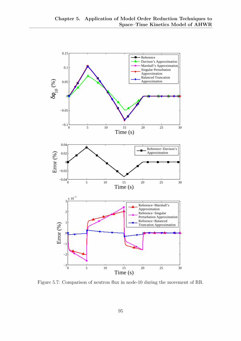
Chapter 5. Application of Model Order Reduction Techniques toSpace–Time Kinetics Model of AHWR
0 5 10 15 20 25 30−0.1
−0.05
0
0.05
0.1
0.15δφ
10 (
%)
Time (s)
ReferenceDavison’s ApproximationMarshall’s ApproximationSingular PerturbationApproximationBalanced TruncationApproximation
0 5 10 15 20 25 30−0.04
−0.02
0
0.02
0.04
Err
or (
%)
Time (s)
Reference−Davison’s Approximation
0 5 10 15 20 25 30−3
−2
−1
0
1
2
3x 10
−3
Err
or (
%)
Time (s)
Reference−Marshall’s ApproximationReference−Singular Perturbation ApproximationReference−Balanced Truncation Approximation
Figure 5.7: Comparison of neutron flux in node-10 during the movement of RR.
95
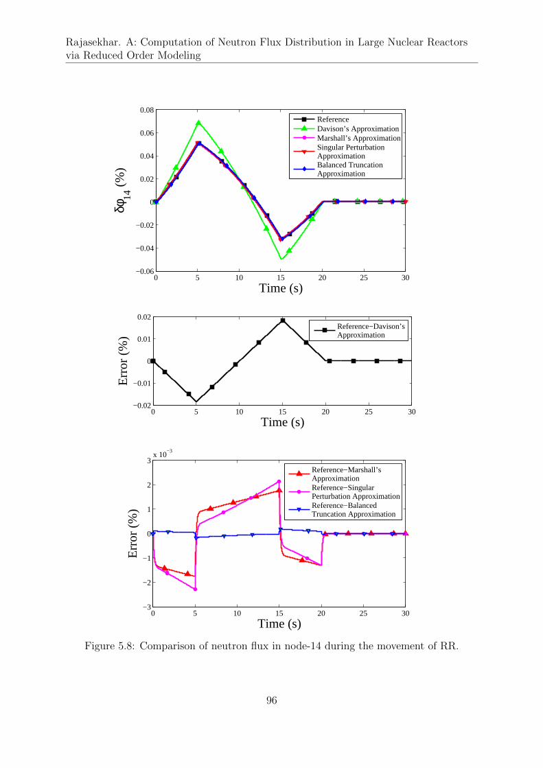
Rajasekhar. A: Computation of Neutron Flux Distribution in Large Nuclear Reactorsvia Reduced Order Modeling
0 5 10 15 20 25 30−0.06
−0.04
−0.02
0
0.02
0.04
0.06
0.08δφ
14 (
%)
Time (s)
ReferenceDavison’s ApproximationMarshall’s ApproximationSingular PerturbationApproximationBalanced TruncationApproximation
0 5 10 15 20 25 30−0.02
−0.01
0
0.01
0.02
Err
or (
%)
Time (s)
Reference−Davison’s Approximation
0 5 10 15 20 25 30−3
−2
−1
0
1
2
3x 10
−3
Err
or (
%)
Time (s)
Reference−Marshall’s ApproximationReference−Singular Perturbation ApproximationReference−Balanced Truncation Approximation
Figure 5.8: Comparison of neutron flux in node-14 during the movement of RR.
96

Chapter 5. Application of Model Order Reduction Techniques toSpace–Time Kinetics Model of AHWR
truncate/reduce. In contrast, singular perturbation techniques require a decomposi-
tion of the state-space systems into fast/slow subsystems using block diagonalization
methods. Davison’s and Marshall’s techniques result into a simplified model that re-
tains the slowly varying dynamics while the application of singular perturbation analysis
and two-time-scale methods decompose the model into two subsystems viz., slow and
fast, thus providing better approximation of dynamics of the system. Quite similar to
this, application of balanced truncation yields a reduced model in which both the slow
and fast dynamic characteristics are simultaneously retained yielding good accuracy in
approximation of high order model by reduced order model.
The order of reduced order model obtained by the application of Davison’s technique
is 22, while that obtained using Marshall’s and singular perturbation techniques both is
21 each, but the balanced truncation technique is the most effective in model reduction
yielding the reduced model of order 10 only. The transient response of simplified models
based on Marshall’s, singular perturbation and balanced truncation techniques were in
good agreement with the transient response of the original high order model.
In summary, we have proposed a novel approach for the application of balanced
truncation technique to nuclear reactor systems which have a nontrivial unstable part
based on stable and unstable decomposition. This is accomplished easily while the
direct application of balanced truncation for model order reduction is not feasible. The
computation involved in obtaining a balanced basis is typically considered too high
and this method has not been adequately used in model order reduction applications.
However, our work shows that the computation is required to be done off-line and only
once. The computation time is only marginally higher, but the advantages outweigh the
marginally higher computation time. It is evidenced that the final reduced order model
based on the balanced truncation method is of much lower order in spite of negligible
error between the response of the original system and that obtained from the reduced
order model. This provides significant advantage from a practical perspective because
a lower-order controller or estimator needs to be designed for the purpose of controlling
97

Rajasekhar. A: Computation of Neutron Flux Distribution in Large Nuclear Reactorsvia Reduced Order Modeling
the AHWR. In general, the singular perturbation and balanced truncation methods are
expected to perform better in cases where time-scales are widely separated.
98
Chapter 6
A Two-time-scale approach for
Discrete-Time Kalman Filter Design
and application to AHWR Flux
Mapping
In this chapter, the task of flux-mapping in THE AHWR has been formulated as linear
stochastic estimation problem and a solution is obtained by Kalman filtering technique.
It utilizes estimation model derived in Section 5.1 and available detector measurements
corrupted with white Gaussian noise. However, direct implementation of the DKF algo-
rithm to this high-order stiff estimation model is not feasible as the designing procedure
is accompanied by serious numerical ill-conditioning caused by the simultaneous pres-
ence of slow and fast phenomena typically present in a nuclear reactor. In particular,
the set of recursive equations for computation of DKF gains, as a solution to weighted
least squares problem, is ill-conditioned. Consequently, serious numerical difficulties are
expected if the DKF gain matrix is to be computed on the basis of the full order Riccati
equation. By using the reduced models based on Davison’s technique, Marshall’s tech-
A part of this chapter was published in IEEE Transactions on Nuclear Science, Vol. 63(1) .
99
Rajasekhar. A: Computation of Neutron Flux Distribution in Large Nuclear Reactorsvia Reduced Order Modeling
nique, singular perturbation analysis and balanced truncation, the estimation model of
lower order can be obtained. Trying all these would be of enormous effort. However, an
attempt has been made to apply the singular perturbation technique which fortunately
is found to work well for the AHWR flux mapping. This chapter presents the proposed
novel technique to address the numerical ill-conditioning problems in full order design
by decoupling the DKF equations according to the order of the slow and fast subsys-
tems. Finally this technique has been applied for estimation of detailed mesh, channel
quadrant and core average fluxes in the AHWR.
6.1 Discrete-Time Kalman Filter Algorithm
The DKF is an optimal recursive data processing algorithm [34, 78], also known as Linear
Quadratic Estimator which uses a series of measurements observed over time, contain-
ing noise (random variations) and other model inaccuracies, and produces estimates of
unknown states that tend to be more precise than those based on a single measurement
alone. From Bayesian point of view, DKF propagates the conditional probability density
of the desired quantities (mean and covariance), conditioned on the knowledge of the
past measurements and updates it when new measurements are available [118]. Consider
a general linear discrete time-invariant stochastic system represented by,
xk = Φxk−1 + Γuk−1 +wk−1, (6.1)
and yk = Ψxk + vk, (6.2)
where k is the discrete-time instant, x ∈ Rn is the state vector, u ∈ Rm is the input vector
and y ∈ Rp is the output vector. Φ ∈ Rn×n, Γ ∈ Rn×m and Ψ ∈ Rp denote the state
transition, input and output matrices respectively. Also, wk and vk are random vectors
representing respectively the process and measurement noise sequences, assumed to be
independent, zero mean, with Gaussian probability distribution and known covariances
100
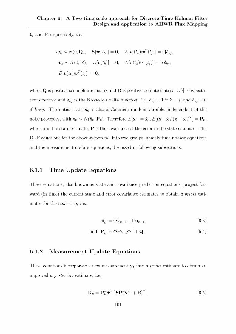
Chapter 6. A Two-time-scale approach for Discrete-Time Kalman FilterDesign and application to AHWR Flux Mapping
Q and R respectively, i.e.,
wk ∼ N(0,Q), E[w(tk)] = 0, E[w(tk)wT (tj)] = Qδkj,
vk ∼ N(0,R), E[v(tk)] = 0, E[v(tk)vT (tj)] = Rδkj,
E[v(tk)wT (tj)] = 0,
where Q is positive-semidefinite matrix and R is positive-definite matrix. E[·] is expecta-
tion operator and δkj is the Kronecker delta function; i.e., δkj = 1 if k = j, and δkj = 0
if k 6=j. The initial state x0 is also a Gaussian random variable, independent of the
noise processes, with x0 ∼ N(x0,P0). Therefore E[x0] = x0, E[(x− x0)(x− x0)T ] = P0,
where x is the state estimate, P is the covariance of the error in the state estimate. The
DKF equations for the above system fall into two groups, namely time update equations
and the measurement update equations, discussed in following subsections.
6.1.1 Time Update Equations
These equations, also known as state and covariance prediction equations, project for-
ward (in time) the current state and error covariance estimates to obtain a priori esti-
mates for the next step, i.e.,
x−k = Φxk−1 + Γuk−1, (6.3)
and P−k = ΦPk−1ΦT + Q. (6.4)
6.1.2 Measurement Update Equations
These equations incorporate a new measurement yk into a priori estimate to obtain an
improved a posteriori estimate, i.e.,
Kk = P−k ΨT [ΨP−k Ψ
T + R]−1, (6.5)
101
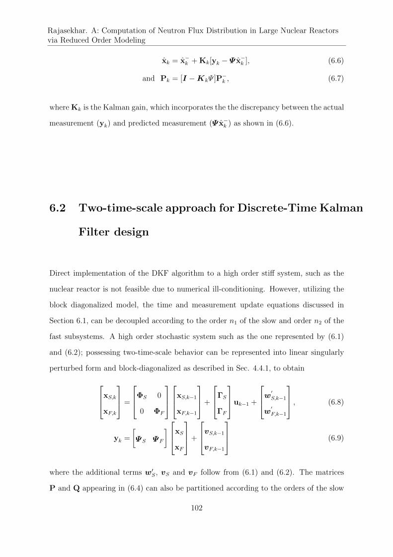
Rajasekhar. A: Computation of Neutron Flux Distribution in Large Nuclear Reactorsvia Reduced Order Modeling
xk = x−k + Kk[yk − Ψ x−k ], (6.6)
and Pk = [I −KkΨ ]P−k , (6.7)
where Kk is the Kalman gain, which incorporates the the discrepancy between the actual
measurement (yk) and predicted measurement (Ψ x−k ) as shown in (6.6).
6.2 Two-time-scale approach for Discrete-Time Kalman
Filter design
Direct implementation of the DKF algorithm to a high order stiff system, such as the
nuclear reactor is not feasible due to numerical ill-conditioning. However, utilizing the
block diagonalized model, the time and measurement update equations discussed in
Section 6.1, can be decoupled according to the order n1 of the slow and order n2 of the
fast subsystems. A high order stochastic system such as the one represented by (6.1)
and (6.2); possessing two-time-scale behavior can be represented into linear singularly
perturbed form and block-diagonalized as described in Sec. 4.4.1, to obtain
xS,k
xF,k
=
ΦS 0
0 ΦF
xS,k−1
xF,k−1
+
ΓS
ΓF
uk−1 +
w′
S,k−1
w′
F,k−1
, (6.8)
yk =
[ΨS ΨF
]xS
xF
+
vS,k−1vF,k−1
(6.9)
where the additional terms w′S, vS and vF follow from (6.1) and (6.2). The matrices
P and Q appearing in (6.4) can also be partitioned according to the orders of the slow
102
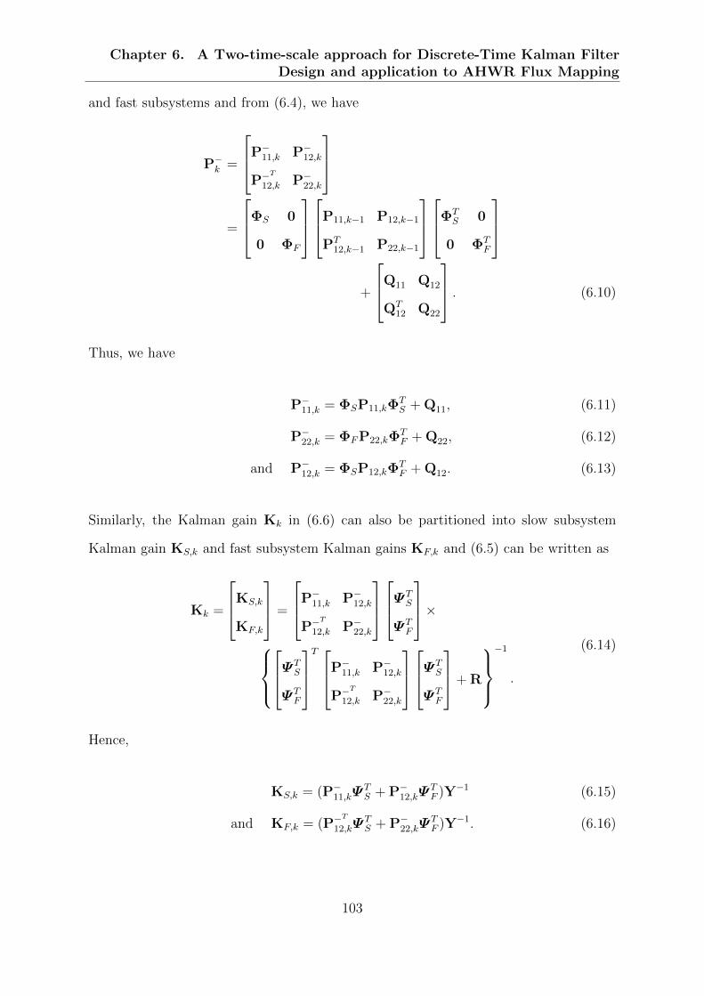
Chapter 6. A Two-time-scale approach for Discrete-Time Kalman FilterDesign and application to AHWR Flux Mapping
and fast subsystems and from (6.4), we have
P−k =
P−11,k P−12,k
P−T
12,k P−22,k
=
ΦS 0
0 ΦF
P11,k−1 P12,k−1
PT12,k−1 P22,k−1
ΦT
S 0
0 ΦTF
+
Q11 Q12
QT12 Q22
. (6.10)
Thus, we have
P−11,k = ΦSP11,kΦTS + Q11, (6.11)
P−22,k = ΦFP22,kΦTF + Q22, (6.12)
and P−12,k = ΦSP12,kΦTF + Q12. (6.13)
Similarly, the Kalman gain Kk in (6.6) can also be partitioned into slow subsystem
Kalman gain KS,k and fast subsystem Kalman gains KF,k and (6.5) can be written as
Kk =
KS,k
KF,k
=
P−11,k P−12,k
P−T
12,k P−22,k
ΨT
S
ΨTF
×ΨT
S
ΨTF
T P−11,k P−12,k
P−T
12,k P−22,k
ΨT
S
ΨTF
+ R
−1
.
(6.14)
Hence,
KS,k = (P−11,kΨTS + P−12,kΨ
TF )Y−1 (6.15)
and KF,k = (P−T
12,kΨTS + P−22,kΨ
TF )Y−1. (6.16)
103
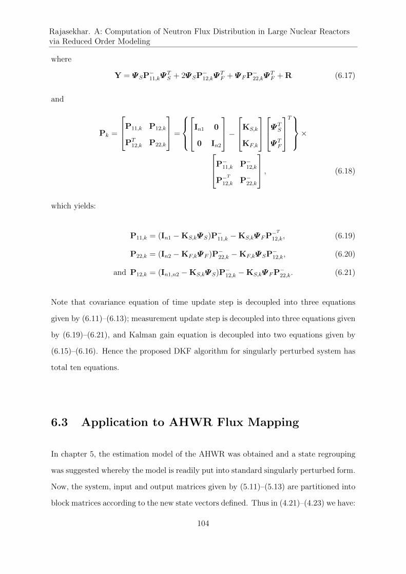
Rajasekhar. A: Computation of Neutron Flux Distribution in Large Nuclear Reactorsvia Reduced Order Modeling
where
Y = ΨSP−11,kΨTS + 2ΨSP−12,kΨ
TF + ΨFP−22,kΨ
TF + R (6.17)
and
Pk =
P11,k P12,k
PT12,k P22,k
=
In1 0
0 In2
−KS,k
KF,k
ΨT
S
ΨTF
T×P−11,k P−12,k
P−T
12,k P−22,k
, (6.18)
which yields:
P11,k = (In1 −KS,kΨS)P−11,k −KS,kΨFP−T
12,k, (6.19)
P22,k = (In2 −KF,kΨF )P−22,k −KF,kΨSP−12,k, (6.20)
and P12,k = (In1,n2 −KS,kΨS)P−12,k −KS,kΨFP−22,k. (6.21)
Note that covariance equation of time update step is decoupled into three equations
given by (6.11)–(6.13); measurement update step is decoupled into three equations given
by (6.19)–(6.21), and Kalman gain equation is decoupled into two equations given by
(6.15)–(6.16). Hence the proposed DKF algorithm for singularly perturbed system has
total ten equations.
6.3 Application to AHWR Flux Mapping
In chapter 5, the estimation model of the AHWR was obtained and a state regrouping
was suggested whereby the model is readily put into standard singularly perturbed form.
Now, the system, input and output matrices given by (5.11)–(5.13) are partitioned into
block matrices according to the new state vectors defined. Thus in (4.21)–(4.23) we have:
104

Chapter 6. A Two-time-scale approach for Discrete-Time Kalman FilterDesign and application to AHWR Flux Mapping
A11 =
0 0
0 ACC
;
A21 =
0 0
AφCH AφCC
;
B1 =
[BTH 0
]T;
Ψ 1 =
[0 0
];
A12 =
0 0
0 ACφC
;
A22 =
AφRφR AφRφC
AφCφR AφCφC
;
B2 =
[0 0
]T;
Ψ 2 =
[0 κDV
].
Now, the full order system is block diagonalized using the similarity transformation
(4.38), in which the L and M matrices for the transformation are obtained by the
iterative solution of (4.41) and (4.42) respectively. Thereafter AS, AF , BS, BF , ΨS
and ΨF of the decoupled system represented by (4.36)–(4.37) are obtained by (4.44).
It is observed that 59 magnitude wise largest eigenvalues of A are equal to eigenvalues
of AF , and the remaining 21 eigenvalues are equal to eigenvalues of AS. This confirms
that the estimation model is decoupled into slow and fast subsystems of order 21 and
59 respectively.
Now the method presented in Section 6.2 has been applied for flux mapping in
the core of AHWR. Estimation model represented by (4.36)–(4.37) is discretized for
sampling time τ = 0.2 s for which the discrete-time system is observed to possess two-
time-scale property. The eigenvalues of discretized system are given in Table 6.1. From
the Table 6.1 , it is evident that discretized model has 21 (S.No.60-S.No.80) eigenvalues
on/around the periphery of the unit circle, and the rest 59 (S.No.1-S.No.59) are inside
the unit circle, which indicates the two-time-scale property in the discrete model.
The effectiveness of the Kalman filtering technique for flux mapping has been ex-
amined in three cases. In the first case, decay of non-zero initial condition is observed.
The states of the estimation model are non-zero while the reactor is assumed to be at
steady–state. In the second, the movement of one or multiple RRs is simulated. Fi-
nally in the third case, xenon-induced spatial oscillation is considered. These cases are
105

Rajasekhar. A: Computation of Neutron Flux Distribution in Large Nuclear Reactorsvia Reduced Order Modeling
elaborated in the following subsections.
SPND signals (measurements) were generated under the same transient situations
from a separate set of off-line computations using a 128-node scheme as shown in Fig.
3.4, for the first two cases, and the 17-node scheme as shown in Fig. 3.3 for the third
case. From the operational 540 MWe PHWR units 3 and 4 of Tarapur Atomic Power
Station (TAPS), India, it was revealed that noise in the signals of detectors takes normal
probability distribution with a standard deviation of nearly 2 % [79]. Hence, measure-
ment noise of the order of 2 % has been assumed for each SPND. This noise is equivalent
to 2 % random fluctuations around the full power steady state–value in each detector.
Using the methodology described in Section 3.4, reference flux values have been
generated for 22950 volume elements, 452 fuel channels, 4 quadrants and the core average
flux denoted respectively as φV , φZ , φQ and φG. The state estimation is carried out
using the DKF algorithm with
Q = 0.1× I80 and R = I200
where I80 and I200 denote identity matrices of size 80 and 200 respectively. Estimates
for fluxes in 22950 volume elements are obtained as
φV = κV xφC, (6.22)
where κV denotes the weighting matrix for flux reconstruction. Now, from the estimates
of flux in 22950 volume elements, the average values of channel fluxes are obtained as
φZ =∑i∈Z
φViVi
/∑i∈Z
Vi, (6.23)
where Vi denotes the volume of the ith mesh box, Z denotes fuel channels in core, as
106

Chapter 6. A Two-time-scale approach for Discrete-Time Kalman FilterDesign and application to AHWR Flux Mapping
Table 6.1: Eigenvalues of discrete-time model for τ = 0.2
S.No Eigenvalue S.No Eigenvalue1 8.9824e− 21 41 1.2527e− 142 1.1967e− 20 42 9.7747e− 143 2.2928e− 20 43 1.2944e− 134 3.1010e− 20 44 1.4448e− 135 5.3019e− 20 45 4.3960e− 136 7.6267e− 19 46 7.0621e− 137 8.2310e− 19 47 1.6174e− 118 8.7412e− 19 48 1.8456e− 119 9.2210e− 19 49 1.2773e− 1010 9.4823e− 19 50 3.6852e− 1011 1.2429e− 19 51 6.4999e− 1012 2.2956e− 19 52 1.1980e− 0913 3.3126e− 19 53 4.7009e− 0914 3.3126e− 19 54 9.5022e− 0915 3.2213e− 19 55 2.3107e− 0716 6.9401e− 19 56 1.0695e− 0617 6.9401e− 19 57 4.2831e− 0418 8.3220e− 19 58 4.8134e− 0419 1.5295e− 18 59 1.8423e− 0120 1.5295e− 18 60 9.8748e− 0121 1.6051e− 18 61 9.8749e− 0122 1.6051e− 18 62 9.8754e− 0123 2.1275e− 18 63 9.8757e− 0124 2.1275e− 18 64 9.8758e− 0125 2.2904e− 18 65 9.8761e− 0126 2.2904e− 18 66 9.8767e− 0127 3.0038e− 18 67 9.8768e− 0128 4.7078e− 18 68 9.8784e− 0129 4.7078e− 18 69 9.8790e− 0130 4.9702e− 18 70 9.8798e− 0131 6.3127e− 18 71 9.8812e− 0132 1.0917e− 17 72 9.8830e− 0133 8.7525e− 17 73 9.8839e− 0134 1.9767e− 16 74 9.8965e− 0135 5.1624e− 15 75 9.8968e− 0136 1.2425e− 15 76 1.0000e+ 0037 1.3603e− 15 77 1.0000e+ 0038 2.3955e− 15 78 1.0000e+ 0039 4.6504e− 15 79 1.0000e+ 0040 6.0565e− 15 80 1.0000e+ 00
107
Rajasekhar. A: Computation of Neutron Flux Distribution in Large Nuclear Reactorsvia Reduced Order Modeling
Table 6.2: Test cases and description
S. No. Test case Description1 1 RR Movement of RR in Q-I, other 3 RRs are stationary2 2 RR Simultaneous movement of RRs in Q-I and Q-III,
other 2 RRs are stationary3 4 RR Simultaneous movement of RRs in Q-I, Q-II, Q-III and Q-IV4 2 RR-D Simultaneous movement of RRs in Q-I and Q-III
in opposite directions, other 2 RRs are stationary
shown in Fig. 3.3. Similarly, the estimated values of quadrant fluxes are computed from
φQ =∑i∈Q
φViVi
/∑i∈Q
Vi, (6.24)
where Q = I, II, III and IV. Estimated value of core average flux is computed as
φG =10848∑i=1
φViVi
/10848∑i=1
Vi. (6.25)
The values of these quantities, as determined using DKF algorithm are compared with
their respective reference values for assessment of reconstruction accuracy.
6.4 Computation of Error
To characterize the performance of the DKF, we compute relative errors in estimation
of flux in 22950 volume elements, 452 coolant channels and 4 quadrants, and also the
error in the estimation of the core average flux, respectively using
eVirel =φVi − φViφVi
× 100, i = 1, 2, ..., 22950; (6.26)
eZirel=φZi− φZi
φZi
× 100, i = 1, 2, ..., 452; (6.27)
108
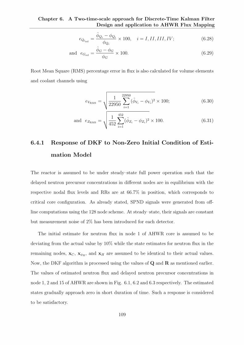
Chapter 6. A Two-time-scale approach for Discrete-Time Kalman FilterDesign and application to AHWR Flux Mapping
eQirel=φQi− φQi
φQi
× 100, i = I, II, III, IV ; (6.28)
and eGrel=φG − φGφG
× 100. (6.29)
Root Mean Square (RMS) percentage error in flux is also calculated for volume elements
and coolant channels using
eVRMS=
√√√√ 1
22950
22950∑i=1
(φVi − φVi)2 × 100; (6.30)
and eZRMS=
√√√√ 1
452
452∑i=1
(φZi− φZi
)2 × 100. (6.31)
6.4.1 Response of DKF to Non-Zero Initial Condition of Esti-
mation Model
The reactor is assumed to be under steady–state full power operation such that the
delayed neutron precursor concentrations in different nodes are in equilibrium with the
respective nodal flux levels and RRs are at 66.7% in position, which corresponds to
critical core configuration. As already stated, SPND signals were generated from off-
line computations using the 128 node scheme. At steady–state, their signals are constant
but measurement noise of 2% has been introduced for each detector.
The initial estimate for neutron flux in node 1 of AHWR core is assumed to be
deviating from the actual value by 10% while the state estimates for neutron flux in the
remaining nodes, xC , xφR , and xH are assumed to be identical to their actual values.
Now, the DKF algorithm is processed using the values of Q and R as mentioned earlier.
The values of estimated neutron flux and delayed neutron precursor concentrations in
node 1, 2 and 15 of AHWR are shown in Fig. 6.1, 6.2 and 6.3 respectively. The estimated
states gradually approach zero in short duration of time. Such a response is considered
to be satisfactory.
109
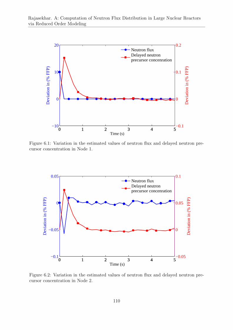
Rajasekhar. A: Computation of Neutron Flux Distribution in Large Nuclear Reactorsvia Reduced Order Modeling
0 1 2 3 4 5−10
0
10
20D
evia
tion
in (
% F
FP
)
Time (s)
0 1 2 3 4 5−0.1
0
0.1
0.2
Dev
iatio
n in
(%
FF
P)
Neutron fluxDelayed neutronprecursor concenration
Figure 6.1: Variation in the estimated values of neutron flux and delayed neutron pre-cursor concentration in Node 1.
0 1 2 3 4 5−0.1
−0.05
0
0.05
Dev
iatio
n in
(%
FF
P)
Time (s)
0 1 2 3 4 5−0.05
0
0.05
0.1
Dev
iatio
n in
(%
FF
P)
Neutron fluxDelayed neutronprecursor concenration
Figure 6.2: Variation in the estimated values of neutron flux and delayed neutron pre-cursor concentration in Node 2.
110

Chapter 6. A Two-time-scale approach for Discrete-Time Kalman FilterDesign and application to AHWR Flux Mapping
0 1 2 3 4 5−0.1
−0.05
0
0.05
0.1D
evia
tion
in (
% F
FP
)
Time (s)
0 1 2 3 4 5−0.1
−0.05
0
0.05
0.1
Dev
iatio
n in
(%
FF
P)
Neutron fluxDelayed neutronprecursor concenration
Figure 6.3: Variation in the estimated values of neutron flux and delayed neutron pre-cursor concentration in Node 15.
Table 6.3: Maximum RMS error in estimation of flux in the transient involving movementRR
S.No. Parameter Error ( %)1 RMS error in estimation of fluxes in 22950 mesh boxes, ezrms 0.30402 RMS error in estimation of fluxes in 452 fuel channels, evrms 0.33813 RMS error in estimation of fluxes in 4 quadrants 0.1592
6.4.2 Movement of Regulating Rods
This simulation involves movement of one or multiple RRs as listed in Table 6.2. At
steady–state full power operation, RRs are at 66.7% in position. In each case, the reactor
is at steady–state for the initial 50 seconds. At time t = 50 s, control signal of 1 V is
applied to RR drive and maintained for 8 s. Corresponding RRs move linearly into the
reactor core, as governed by (3.22) and reach 71.14% in position. Then, control signal is
made 0 V to hold the RRs at the new position. After 3 s, the RR is driven out linearly
to nominal position by applying a control signal of −1 V. Again after 3 s, an outward
movement followed by inward movement back to its nominal position is simulated.
First, movement of RR located in Quadrant-I is considered. Fig. 6.4 shows the
111
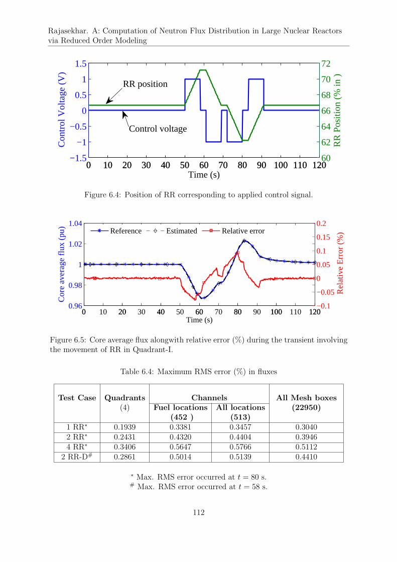
Rajasekhar. A: Computation of Neutron Flux Distribution in Large Nuclear Reactorsvia Reduced Order Modeling
0 10 20 30 40 50 60 70 80 90 100 110 120−1.5
−1
−0.5
0
0.5
1
1.5C
ontr
ol V
olta
ge (
V)
Time (s)0 10 20 30 40 50 60 70 80 90 100 110 120
60
62
64
66
68
70
72
RR
Pos
ition
(%
in )
Control voltage
RR position
Figure 6.4: Position of RR corresponding to applied control signal.
0 10 20 30 40 50 60 70 80 90 100 110 1200.96
0.98
1
1.02
1.04
Cor
e av
erag
e flu
x (p
u)
Time (s)
0 20 40 60 80 100 120−0.1
−0.05
0
0.05
0.1
0.15
0.2
Rel
ativ
e E
rror
(%
)Reference Estimated Relative error
Figure 6.5: Core average flux alongwith relative error (%) during the transient involvingthe movement of RR in Quadrant-I.
Table 6.4: Maximum RMS error (%) in fluxes
Test Case Quadrants All Mesh boxes(4)
Channels(22950)Fuel locations All locations
(452 ) (513)1 RR∗ 0.1939 0.3381 0.3457 0.30402 RR∗ 0.2431 0.4320 0.4404 0.39464 RR∗ 0.3406 0.5647 0.5766 0.5112
2 RR-D# 0.2861 0.5014 0.5139 0.4410
∗ Max. RMS error occurred at t = 80 s.# Max. RMS error occurred at t = 58 s.
112

Chapter 6. A Two-time-scale approach for Discrete-Time Kalman FilterDesign and application to AHWR Flux Mapping
0 10 20 30 40 50 60 70 80 90 100 110 1200.94
0.98
1.02
1.06
Ave
rage
flux
in Q
uadr
ant−
I (pu
)
Time (s)
0 20 40 60 80 100 120−0.4
0
0.4
0.8
1.2
Rel
ativ
e E
rror
(%
)
Reference Estimated Relative error
0 10 20 30 40 50 60 70 80 90 100 110 1200.94
0.98
1.02
1.06
Ave
rage
flux
in Q
uadr
ant−
II (p
u)
Time (s)
0 20 40 60 80 100 120−0.05
0
0.05
0.1
0.15
Rel
ativ
e E
rror
(%
)
Reference Estimated Relative error
0 10 20 30 40 50 60 70 80 90 100 110 1200.94
0.98
1.02
1.06
Ave
rage
flux
in Q
uadr
ant−
III (
pu)
Time (s)
0 20 40 60 80 100 120−0.05
0
0.05
0.1
0.15
Rel
ativ
e E
rror
(%
)
Reference Estimated Relative error
0 10 20 30 40 50 60 70 80 90 100 110 1200.94
0.98
1.02
1.06
Ave
rage
flux
in Q
uadr
ant−
IV (
pu)
Time (s)
0 20 40 60 80 100 120−0.1
−0.05
0
0.05
0.1
0.15
Rel
ativ
e E
rror
(%
)
Reference Estimated Relative error
Figure 6.6: Average flux in Quadrants I, II, III and IV during the transient involvingthe movement of RR in quadrant-I.
113
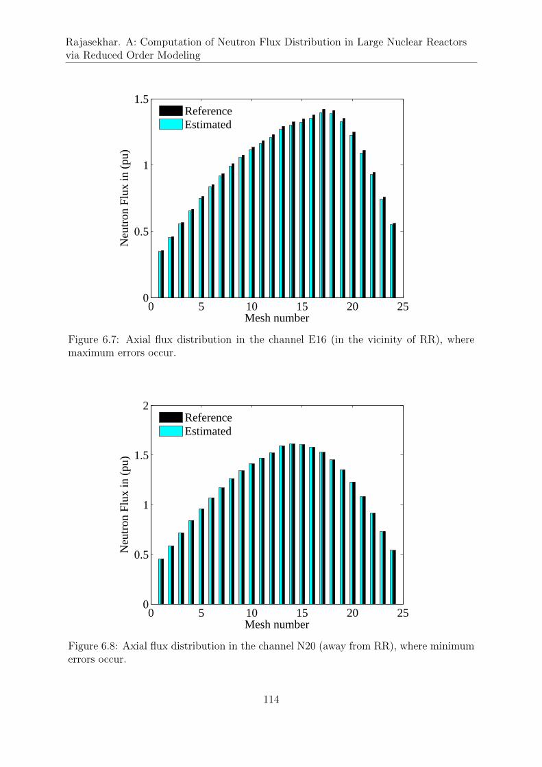
Rajasekhar. A: Computation of Neutron Flux Distribution in Large Nuclear Reactorsvia Reduced Order Modeling
0 5 10 15 20 250
0.5
1
1.5
Mesh number
Neu
tron
Flu
x in
(pu
)
ReferenceEstimated
Figure 6.7: Axial flux distribution in the channel E16 (in the vicinity of RR), wheremaximum errors occur.
0 5 10 15 20 250
0.5
1
1.5
2
Mesh number
Neu
tron
Flu
x in
(pu
)
ReferenceEstimated
Figure 6.8: Axial flux distribution in the channel N20 (away from RR), where minimumerrors occur.
114

Chapter 6. A Two-time-scale approach for Discrete-Time Kalman FilterDesign and application to AHWR Flux Mapping
0
10
20
30
0
10
20
300
0.2
0.4
0.6
0.8
X latticeY lattice
Neu
tron
Flu
x in
(p.
u)
0
0.1
0.2
0.3
0.4
0.5
0.6
Horizontal Plane 1
0
10
20
30
0
10
20
300
0.5
1
1.5
2
X latticeY lattice
Neu
tron
Flu
x in
(p.
u)
0.2
0.4
0.6
0.8
1
1.2
1.4
1.6
1.8
Horizontal Plane 12
0
10
20
30
0
10
20
300
0.2
0.4
0.6
0.8
X latticeY lattice
Neu
tron
Flu
x in
(p.
u)
0.1
0.2
0.3
0.4
0.5
0.6
Horizontal Plane 24
Figure 6.9: 3-D flux distribution in horizontal planes z=1, z=12 and z=24 at t = 0 s.
115

Rajasekhar. A: Computation of Neutron Flux Distribution in Large Nuclear Reactorsvia Reduced Order Modeling
0
10
20
30
0
10
20
300
0.2
0.4
0.6
0.8
X latticeY lattice
Neu
tron
Flu
x in
(p.
u)
0.1
0.2
0.3
0.4
0.5
0.6
Horizontal plane 1
0
10
20
30
0
10
20
300
0.5
1
1.5
2
X latticeY lattice
Neu
tron
Flu
x in
(p.
u)
0
0.2
0.4
0.6
0.8
1
1.2
1.4
1.6
1.8
Horizontal plane 12
0
10
20
30
0
10
20
300
0.2
0.4
0.6
0.8
X latticeY lattice
Neu
tron
Flu
x in
(p.
u)
0.1
0.2
0.3
0.4
0.5
0.6
Horizontal plane 24
Figure 6.10: 3-D flux distribution in horizontal planes z=1, z=12 and z=24 at t = 80 s.
116
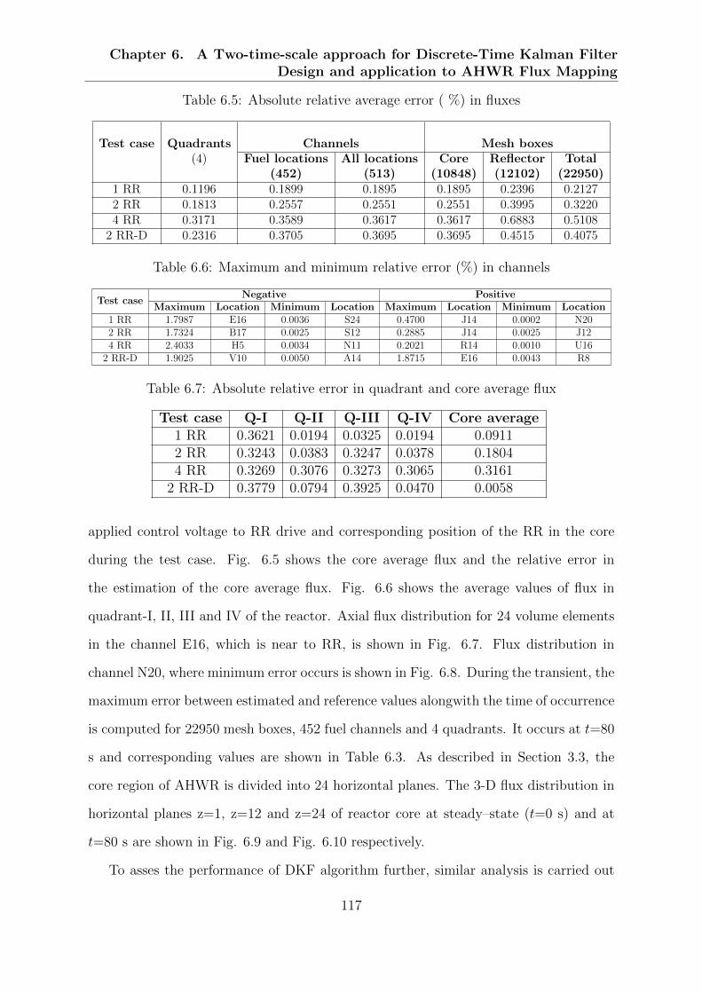
Chapter 6. A Two-time-scale approach for Discrete-Time Kalman FilterDesign and application to AHWR Flux Mapping
Table 6.5: Absolute relative average error ( %) in fluxes
Test case Quadrants(4)
Channels Mesh boxesFuel locations All locations Core Reflector Total
(452) (513) (10848) (12102) (22950)1 RR 0.1196 0.1899 0.1895 0.1895 0.2396 0.21272 RR 0.1813 0.2557 0.2551 0.2551 0.3995 0.32204 RR 0.3171 0.3589 0.3617 0.3617 0.6883 0.5108
2 RR-D 0.2316 0.3705 0.3695 0.3695 0.4515 0.4075
Table 6.6: Maximum and minimum relative error (%) in channels
Test caseNegative Positive
Maximum Location Minimum Location Maximum Location Minimum Location1 RR 1.7987 E16 0.0036 S24 0.4700 J14 0.0002 N202 RR 1.7324 B17 0.0025 S12 0.2885 J14 0.0025 J124 RR 2.4033 H5 0.0034 N11 0.2021 R14 0.0010 U16
2 RR-D 1.9025 V10 0.0050 A14 1.8715 E16 0.0043 R8
Table 6.7: Absolute relative error in quadrant and core average flux
Test case Q-I Q-II Q-III Q-IV Core average1 RR 0.3621 0.0194 0.0325 0.0194 0.09112 RR 0.3243 0.0383 0.3247 0.0378 0.18044 RR 0.3269 0.3076 0.3273 0.3065 0.3161
2 RR-D 0.3779 0.0794 0.3925 0.0470 0.0058
applied control voltage to RR drive and corresponding position of the RR in the core
during the test case. Fig. 6.5 shows the core average flux and the relative error in
the estimation of the core average flux. Fig. 6.6 shows the average values of flux in
quadrant-I, II, III and IV of the reactor. Axial flux distribution for 24 volume elements
in the channel E16, which is near to RR, is shown in Fig. 6.7. Flux distribution in
channel N20, where minimum error occurs is shown in Fig. 6.8. During the transient, the
maximum error between estimated and reference values alongwith the time of occurrence
is computed for 22950 mesh boxes, 452 fuel channels and 4 quadrants. It occurs at t=80
s and corresponding values are shown in Table 6.3. As described in Section 3.3, the
core region of AHWR is divided into 24 horizontal planes. The 3-D flux distribution in
horizontal planes z=1, z=12 and z=24 of reactor core at steady–state (t=0 s) and at
t=80 s are shown in Fig. 6.9 and Fig. 6.10 respectively.
To asses the performance of DKF algorithm further, similar analysis is carried out
117
Rajasekhar. A: Computation of Neutron Flux Distribution in Large Nuclear Reactorsvia Reduced Order Modeling
for the remaining test cases listed in Table 6.2. RMS error between estimated and
reference distribution were computed and are shown in Table 6.4. At the instant when
the maximum RMS error occurred, absolute relative average errors (%) in fluxes are
computed and shown in Table 6.5. Channelwise maximum and minimum relative errors
(%) are shown in Table 6.6. Absolute relative error in quadrant fluxes and core average
fluxes are also computed and shown in Table 6.7.
It is worthy to note from the numerical values presented in Table 6.4–6.7, that the
average relative error and maximum RMS error in quadrant fluxes are 0.31% and 0.34%
respectively; in case of channel fluxes they are 0.37% and 0.57% respectively; and in the
case of mesh fluxes they are 0.37% and 0.51% respectively. These are of the same order
as reported in [52, 71]. From the Table 6.6 it can be claimed that the maximum relative
error in the estimation of channel flux from the DKF method is 2.4%. This is of the
same order as reported in elsewhere, e.g., in [47], but the DKF has been evaluated for
transient situations.
6.4.3 Xenon-Induced Oscillations
As already stated, due to large physical dimensions, operational perturbations might lead
to slow xenon induced-oscillations in AHWR. If these oscillations are left uncontrolled,
the power density and time rate of change of power at some locations in the reactor core
may exceed the respective design limits, resulting into increased chance of fuel failure.
Therefore, to maintain the total power and power distribution within the design limits,
AHWR is provided with total power control and spatial power control schemes. If due
to some hypothetical reason, the spatial control scheme is ineffective, xenon-induced
oscillations might occur. These xenon-induced spatial oscillations and subsequent local
overpowers pose a potential threat to the fuel integrity of the reactor. Therefore, the
detailed knowledge of axial and radial flux distribution in the core during the operational
condition is crucial.
118
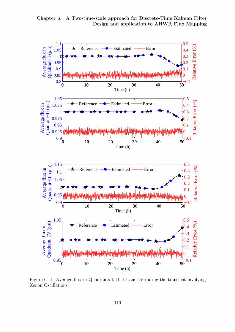
Chapter 6. A Two-time-scale approach for Discrete-Time Kalman FilterDesign and application to AHWR Flux Mapping
0 10 20 30 40 500.8
0.85
0.9
0.95
1
1.05
1.1A
vera
ge fl
ux in
Qua
dran
t−I (
p.u)
Time (h)
0 10 20 30 40 50−0.1
0
0.1
0.2
0.3
0.4
0.5
Rel
ativ
e E
rror
(%
)
Reference Estimated Error
0 10 20 30 40 500.9
0.925
0.95
0.975
1
1.025
1.05
Ave
rage
flux
in Q
uadr
ant−
II (p
.u)
Time (h)
0 10 20 30 40 50−0.1
0
0.1
0.2
0.3
0.4
0.5
Rel
ativ
e E
rror
(%
)
Reference Estimated Error
0 10 20 30 40 500.9
0.95
1
1.05
1.1
1.15
Ave
rage
flux
in Q
uadr
ant−
III (
p.u)
Time (h)
0 10 20 30 40 50−0.1
0
0.1
0.2
0.3
0.4
0.5
Rel
ativ
e E
rror
(%
)
Reference Estimated Error
0 10 20 30 40 500.95
1
1.05
Ave
rage
flux
in Q
uadr
ant−
IV (
p.u)
Time (h)
0 10 20 30 40 50−0.1
0
0.1
0.2
0.3
0.4
0.5
Rel
ativ
e E
rror
(%
)
Reference Estimated Error
Figure 6.11: Average flux in Quadrants I, II, III and IV during the transient involvingXenon Oscillations.
119
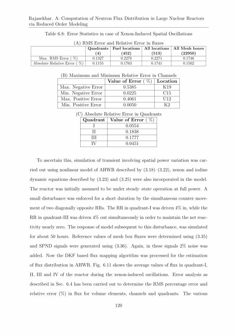
Rajasekhar. A: Computation of Neutron Flux Distribution in Large Nuclear Reactorsvia Reduced Order Modeling
Table 6.8: Error Statistics in case of Xenon-Induced Spatial Oscillations
(A) RMS Error and Relative Error in fluxesQuadrants Fuel locations All locations All Mesh boxes
(4) (452) (513) (22950)Max. RMS Error ( %) 0.1327 0.2278 0.2271 0.1746
Absolute Relative Error ( %) 0.1155 0.1763 0.1741 0.1502
(B) Maximum and Minimum Relative Error in ChannelsValue of Error ( %) Location
Max. Negative Error 0.5385 K19Min. Negative Error 0.0225 C15Max. Positive Error 0.4061 U12Min. Positive Error 0.0050 K2
(C) Absolute Relative Error in QuadrantsQuadrant Value of Error ( %)
I 0.0554II 0.1838III 0.1777IV 0.0451
To ascertain this, simulation of transient involving spatial power variation was car-
ried out using nonlinear model of AHWR described by (3.18)–(3.22), xenon and iodine
dynamic equations described by (3.23) and (3.25) were also incorporated in the model.
The reactor was initially assumed to be under steady–state operation at full power. A
small disturbance was enforced for a short duration by the simultaneous counter move-
ment of two diagonally opposite RRs. The RR in quadrant-I was driven 4% in, while the
RR in quadrant-III was driven 4% out simultaneously in order to maintain the net reac-
tivity nearly zero. The response of model subsequent to this disturbance, was simulated
for about 50 hours. Reference values of mesh box fluxes were determined using (3.35)
and SPND signals were generated using (3.36). Again, in these signals 2% noise was
added. Now the DKF based flux mapping algorithm was processed for the estimation
of flux distribution in AHWR. Fig. 6.11 shows the average values of flux in quadrant-I,
II, III and IV of the reactor during the xenon-induced oscillations. Error analysis as
described in Sec. 6.4 has been carried out to determine the RMS percentage error and
relative error (%) in flux for volume elements, channels and quadrants. The various
120
Chapter 6. A Two-time-scale approach for Discrete-Time Kalman FilterDesign and application to AHWR Flux Mapping
types of errors in estimation are given in Table 6.8. In general, the errors are observed
to be insignificant.
From the simulations, it can be concluded that, the proposed DKF algorithm can
accurately estimate the time dependent neutron flux distribution during the typical
reactor operating conditions. The degradation of DKF algorithm accuracy is also very
less against the detector random errors.
6.5 Discussion
In this chapter, the task of flux mapping problem in the AHWR has been formulated as
a problem of optimally estimating the time dependent neutron flux at a large number of
mesh points in the core. The solution is obtained using the well known Kalman filtering
technique which works alongwith a space–time kinetics model of the reactor. However,
the attempt to solve the Kalman filtering problem in a straight forward manner is not
successful due to severe numerical ill-conditioning caused by the simultaneous presence
of slow and fast phenomena, typically present in a nuclear reactor. Hence, a grouping of
state variables has been suggested whereby the original high order model of the reactor
is decoupled into a slow subsystem and a fast subsystem. Now according to order of
the slow and fast subsystems, the original time update and Kalman gain equations have
also been decoupled into separate sets of equations for the slow and fast subsystems.
The decoupled sets of equations could be solved easily. The proposed method has been
validated in a number of typical transient situations. Overall accuracy in the estimation
using the proposed methodology has been very good for mesh fluxes, channel fluxes,
quadrant fluxes and the core average flux. Therefore, the proposed method can serve
an effective alternate to the existing flux mapping techniques.
121
Chapter 7
Conclusions and Future Scope
The neutron flux distribution in a large nuclear reactor undergoes continuous varia-
tion due to routine perturbations, non-uniform burn up at different locations, etc. The
operating procedure and core control philosophy generally ensure that the time depen-
dent flux variations are maintained within prescribed limits. However, the flux profile
is continuously monitored and displayed to operator. The knowledge of flux distribu-
tion in the reactor core during its operation is helpful to the operator in planning of
refueling scheme as well as in zonal power correction. Therefore, for safe, reliable and
economic operation these large nuclear reactor cores should be provided with online
spatial flux/power distribution monitoring schemes during the course of operation. This
has been the motivating factor for pursuing the type of research work presented in this
thesis. More specifically, the flux mapping problem of the 920 MW (thermal) AHWR
as a particular case of study has been accomplished in this thesis.
The time varying neutron flux distribution in nuclear reactor is computed by an
online FMS, with the help of flux mapping algorithms. The measurement signals of
several in-core SPND detectors are processed to generate the detailed three dimensional
flux map, which helps for spatial control purpose. These measurement signals are cor-
rupted by random noise, which is inevitable. Existing flux mapping algorithms for online
computation of flux/power distribution suffer from a drawback that they might fail to
122

Chapter 7. Conclusions and Future Scope
account for the time variation of neutron flux and the accuracy of mapping might be
degraded in presence of uncertainty in the detector readings. Recent trends and devel-
opments in state estimation theory, modern control system theory (state-space analy-
sis) provide us with systematic method for designing an efficient optimal flux mapping
algorithm based on Kalman filtering technique for the AHWR, which has significant
importance in practical online application. This has been the other important factor for
the research work reported in this thesis.
For the AHWR, an estimation model has been derived for flux mapping computa-
tions. The nonlinear mathematical model (core neutronics and control rod dynamics
equations) is linearized around the steady–state full power operation by considering a
small perturbation in the system and then the equations are cast into standard state-
space form. It is characterized by 80 states, 4 inputs and 200 outputs. From the
spectrum of eigenvalues of the estimation model, it has been observed that model is as-
sociated with two-time scale property. The direct implementation of the DKF algorithm
to this high-order stiff estimation model is not feasible as the designing procedure is ac-
companied by serious numerical ill-conditioning caused by the simultaneous presence of
slow and fast phenomena typically present in a nuclear reactor. In particular, the set
of recursive equations for computation of DKF gains, as a solution to weighted least
squares problem, is ill-conditioned. Application of the model order reduction techniques
alleviates the numerical ill-conditioning.
Simplified models alleviating the high dimensionality as well as numerical ill-conditioning
can be obtained with the application of model order reduction techniques. Application of
model order reduction techniques preserve the important dynamic characteristics of the
estimation model, while certain less important characteristics are ignored. In particular,
for the AHWR estimation model the application of Davison’s and Marshall’s dominant
mode retention techniques; balanced truncation technique and model decomposition into
slow and fast subsystems based on singular perturbation analysis have been explored.
All of these four methods are found to be effective in obtaining simplified models of
123
Rajasekhar. A: Computation of Neutron Flux Distribution in Large Nuclear Reactorsvia Reduced Order Modeling
AHWR. However, reduced order model based on the balanced truncation method is of
much lower order in spite of negligible error between the response of the original system
and that obtained from the reduced order model.
Application of methods based on retention of dominant modes requires diagonaliza-
tion. For the estimation model, it is quite difficult task to get the model into diagonal
form as there are multiple eigenvalues at the origin of the complex s-plane. This is due
to the fact that the model contains slow control rod dynamics. In this thesis, a system-
atic method has been suggested to handle the numerical ill-conditioning occurring in the
computations due to the presence of the slow control rod dynamics by decoupling the
higher order model into slow and fast models. Model order reduction techniques based
on Davison’s and Marshall’s dominant mode retention are then applied to retain the
slow dynamics. Finally the reduced order model has been formulated by augmenting
the control rod dynamics to the model corresponding to the slow dynamics. In this the-
sis, a novel approach for the application of balanced truncation technique to estimation
model having nontrivial unstable part based on stable and unstable decomposition has
also been suggested. This is accomplished easily while the direct application of balanced
truncation for model order reduction is not feasible.
Due to the two-time-scale behavior, revealed by AHWR, direct implementation of
DKF algorithm is not feasible as the design procedure is accompanied by serious nu-
merical ill-conditioning issues. Therefore, the estimation model of AHWR has been de-
composed into slow and fast subsystems based on singular perturbation analysis (block
diagonalization) by suggesting a regrouping of state variables. Then, according to the
order of the slow and fast subsystems, the original time update and Kalman gain equa-
tions have also been decoupled into separate sets of equations for the slow and fast
subsystems. The decoupled sets of equations could be solved easily and efficiently.
The important aspect of the proposed DKF technique is that it attempts solving for
smaller order state prediction equations, process covariance matrices and Kalman gain.
Moreover, it yields excellent accuracy in flux estimation as evident from simulation
124
Chapter 7. Conclusions and Future Scope
exercises. For validation of different techniques of flux mapping, computation results
generated using a high fidelity model is a necessity. Hence, a model based on 128-nodes
in the core resulting into 1168 th order has also been developed.
Feasibility of Kalman filtering technique to the estimation of time varying neutron
flux distribution in AHWR has been successfully explored in this thesis. It also leads to
some future directions for research. Advanced state of the art approaches of estimation
such as EKF, UKF etc., also can be applied to the same problem. Optimality and the
availability of the DKF based flux mapping algorithm can also be verified under the
faults in some detectors. In addition to this, a reduced order DKF can be designed
based on the simplified model obtained from the balanced truncation approach for the
estimation of core flux distribution in AHWR in future.
Before deployment in the AHWR, the efficacy of the technique needs to be established
further, and it should be demonstrated using plant data, such as from PHWRs that it
yields improvement in accuracy compared to that resulting from existing techniques. It
should also be assessed from the viewpoint of implementation that the computations
could be performed in real-time using hardware and other resources, suitable for control
and instrumentation systems in nuclear reactors.
125
References
[1] DESIGN BASIS REPORT ON FLUX MAPPING SYSTEM.
AHWR/DBR/637/63715/0. Rev.0.
[2] A. C. Antoulas. Approximation of Large-Scale Dynamical Systems. Advances in
Design and Control. SIAM, Philadelphia, 2005.
[3] M. Aoki. Control of large-scale dynamic systems by aggregation. IEEE Trans.
Autom. Control, 13(3):246–253, 1968.
[4] P. Benner, V. Mehrmann, and D. C. Sorensen. Dimension reduction of large-scale
systems, volume 45. Lecture Notes in Computational Science and Engineering.
Springer, Berlin, 2005.
[5] P. Benner, E. S. Quintana-Ortı, and G. Quintana-Ortı. State-space truncation
methods for parallel model reduction of large-scale systems. Parallel Computing,
29(11):1701–1722, 2003.
[6] T. U. Bhatt, S. R. Shimjith, A. P. Tiwari, K. P. Singh, S. K. Singh, K. Singh,
and R. K. Patil. Estimation of sub-criticality using extended kalman filtering
technique. Ann. Nucl. Energy, 60:98–105, 2013.
[7] R. Bonalumi and N. Kherani. Rational mapping (ram) of in-core data. Nucl. Sci.
and Eng.g, 90:47, 1985.
[8] J. W. Bryson, J. C. Lee, and J. A. Hassberger. Optimal flux map genera-
126
References
tion through parameter estimation techniques. Nuclear science and engineering,
114(3):238–251, 1993.
[9] K. W. Chang. Singular perturbations of a general boundary value problem. SIAM
Journal on Mathematical Analysis, 3(3):520–526, 1972.
[10] C. F. Chen and L. S. Shieh. A novel approach to linear model simplification.
International Journal of Control, 8(6):561–570, 1968.
[11] T. C. Chen, C. Y. Chang, and K. W. Han. Reduction of transfer functions by
the stability-equation method. Journal of the Franklin Institute, 308(4):389–404,
1979.
[12] J. H. Chow and P. V. Kokotovic. A decomposition of near-optimum regulators for
systems with slow and fast modes. IEEE Trans. on Autom. Contr., 21(5):701–705,
1976.
[13] F. E. Daum and R. J. Fitzgerald. Decoupled kalman filters for phased array radar
tracking. IEEE Trans. Autom. Control, 28(3):269–283, 1983.
[14] E. J. Davison. A method for simplifying linear dynamic systems. IEEE Trans.
Autom. Control, 11(1):93–101, 1966.
[15] E. J. Davison. Further comments on “a method for simplifying linear dynamic
systems”. IEEE Trans. Autom. Control, 12(6):799–800, 1967.
[16] E. J. Davison. Further remarks on simplifying linear dynamic systems. IEEE
Trans. Autom. Control, 12(2):213–214, 1967.
[17] E. J. Davison. On “a method for simplifying linear dynamic systems”. IEEE
Trans. Autom. Control, 12(1):119–121, 1967.
[18] E. J. Davison. A new method for simplifying large linear dynamic systems. IEEE
Trans. Autom. Control, 13(2):214–215, 1968.
127
Rajasekhar. A: Computation of Neutron Flux Distribution in Large Nuclear Reactorsvia Reduced Order Modeling
[19] J. J. Duderstadt and L. J. Hamilton. Nuclear reactor analysis. John Wiley and
Sons, New York, 1976.
[20] Z. Elrazaz and N. K. Sinha. On the selection of the dominant poles of a system
to be retained in a low-order model. IEEE Trans. Autom. Control, 24(5):792–793,
1979.
[21] D. F. Enns. Model reduction with balanced realizations: An error bound and a
frequency weighted generalization. In Decision and Control, 1984. The 23rd IEEE
Conference on, pages 127–132. IEEE, 1984.
[22] W. H. Enright and M. S. Kamel. On selecting a low-order model using the domi-
nant mode concept. IEEE Trans. Autom. Control, 25(5):976–978, 1980.
[23] H. EZURE. Estimation of most probable power distribution in BWRs by least
squares method using in-core measurements. J. of Nucl. Sci. and Tech., 25(9):731–
740, 1988.
[24] R. J. Fitzgerald. Divergence of the Kalman filter. IEEE Trans. Autom. Control,
16(6):736–747, 1971.
[25] L. Fortuna, G. Nunnari, and A. Gallo. Model Order Reduction Techniques with
Applications in Electrical Engineering. Springer Science & Business Media, 1992.
[26] A. Fossard. On a method for simplifying linear dynamic systems. IEEE Trans.
Autom. Control, 15(2):261–262, 1970.
[27] L. Fu, L. Zhengpei, and H. Yongming. Harmonics synthesis method for core flux
distribution reconstruction. Prog. in Nucl. Energy, 31(4):369–372, 1997.
[28] Z. Gajic. Numerical fixed-point solution for near-optimum regulators of linear
quadratic gaussian control problems for singularly perturbed systems. Interna-
tional Journal of Control, 43(2):373–387, 1986.
128
References
[29] Z. Gajic. Optimal control of singularly perturbed linear systems and applications.
CRC Press, 2001.
[30] Z. Gajic, M. T. Lim, and X. Shen. The study of discrete singularly perturbed
linear-quadratic control systems. Control and Dynamic Systems, 70(C):199–242,
1995.
[31] Z. Gajic and X. Shen. Parallel reduced-order controllers for stochastic linear sin-
gularly perturbed discrete systems. Automatic Control, IEEE Transactions on,
36(1):87–90, 1991.
[32] Z. Gajic and X. S. Shen. Parallel algorithms for optimal control of large scale
linear systems. Springer-Verlag London, 1993.
[33] C. F. Gauss. Theory of the motion of the heavenly bodies moving about the sun
in conic sections: a translation of Carl Frdr. Gauss” Theoria motus corporum
coelestium”: With an appendix. By Ch. H. Davis. Little, Brown and Comp., 1857.
[34] A. Gelb. Applied Optimal Estimation. MIT Press, 1974.
[35] R. Genesio and M. Milanese. A note on the derivation and use of reduced-order
models. IEEE Trans. Autom. Control, 21(1):118–122, 1976.
[36] A. Ghafoor and V. Sreeram. A survey/review of frequency-weighted balanced
model reduction techniques. Journal of Dynamic Systems, Measurement, and
Control, 130(6):061004, 2008.
[37] S. Glasstone and A. Sesonske. Nuclear reactor engineering: reactor systems engi-
neering. Springer Science & Business Media, 2012.
[38] K. Glover. All optimal Hankel-norm approximations of linear multivariable sys-
tems and their L∞-error bounds. International journal of control, 39(6):1115–1193,
1984.
129
Rajasekhar. A: Computation of Neutron Flux Distribution in Large Nuclear Reactorsvia Reduced Order Modeling
[39] M. Gopal and S. Mehta. On the selection of the eigenvalues to be retained in the
reduced order models. Automatic Control, IEEE Transactions on, 27(3):688–690,
1982.
[40] K. M. Grigoriadis. Optimal H∞ model reduction via linear matrix inequalities:
continuous and discrete-time cases. In proceedings of the 34th IEEE Conference
on Decision and Control, 1995, volume 3, pages 3074–3079. IEEE, 1995.
[41] L. M. Grossman and J. P. Hennart. Nodal diffusion methods for space-time neutron
kinetics. Progress in Nuclear Energy, 49(3):181–216, 2007.
[42] S. Gugercin and A. C. Antoulas. A survey of model reduction by balanced trun-
cation and some new results. International Journal of Control, 77(8):748–766,
2004.
[43] A. Haddad. Linear filtering of singularly perturbed systems. Automatic Control,
IEEE Transactions on, 21(4):515–519, 1976.
[44] A. Haddad and P. Kokotovic. Stochastic control of linear sigularly perturbed
systems. Automatic Control, IEEE Transactions on, 22(5):815–821, 1977.
[45] H. Hamidi-Hashemi and C. Leondes. Reduction of high-order discrete-time sys-
tems. International journal of systems science, 19(9):1883–1890, 1988.
[46] E. Hinchley and G. Kugler. On-line control of the CANDU PHW power distribu-
tion. In IAEA Specialists Meet. on Spatial Control Problems, Studsvik, Sweden,
oct., 1974.
[47] I. S. Hong, C. H. Kim, and H. C. Suk. Advanced Online Flux Mapping of CANDU
PHWR by Least-Squares Method. Nucl. Sci and Engg., 150(3):299–309, 2005.
[48] M. F. Hutton. Routh approximation method and singular perturbations. In An-
nual Allerton Conference on Circuit and System Theory, 13 th, Monticello, Ill,
pages 29–38, 1976.
130
References
[49] M. F. Hutton and B. Friedland. Routh approximations for reducing order of linear,
time-invariant systems. IEEE Trans. Autom. Control, 20(3):329–337, 1975.
[50] H. Ikeda and T. Takeda. Development and verification of an efficient spatial
neutron kinetics method for reactivity-initiated event analyses. Journal of nuclear
science and technology, 38(7):492–502, 2001.
[51] Z. IWAI and Y. KUBO. Determination of eigenvalues in marshall’s model reduc-
tion. International Journal of Control, 30(5):823–836, 1979.
[52] C. J. Jeong and N. Z. Cho. Power Mapping in a Canada Deuterium Uranium
Reactor Using Kalman Filtering Technique. J. of Nucl. Sci. and Tech., 37(9):758–
768, 2000.
[53] R. E. Kalman. A new approach to linear filtering and prediction problems. Journal
of Fluids Engineering, 82(1):35–45, 1960.
[54] R. E. Kalman. Toward a theory of difficulty of computation in optimal control.
In proc. IBM Scientific Comput. Symp. on Contr. Theory and Appl., 1966.
[55] H. Kando. State estimation of stochastic singularly perturbed discrete-time sys-
tems. Optimal Control Applications and Methods, 18(1):15–28, 1997.
[56] S. Kaplan, O. Marlowe, and J. Bewick. Application of synthesis techniques to
problems involving time dependence. Nuclear Science and Engineering, 18(2):163–
176, 1964.
[57] C. Kenney and G. Hewer. Necessary and sufficient conditions for balancing un-
stable systems. IEEE Trans. Autom. Control, 32(2):157–160, 1987.
[58] H. Khalil and Z. Gajic. Near-optimum regulators for stochastic linear singularly
perturbed systems. Automatic Control, IEEE Transactions on, 29(6):531–541,
1984.
131
Rajasekhar. A: Computation of Neutron Flux Distribution in Large Nuclear Reactorsvia Reduced Order Modeling
[59] H. KOKAME and Y. HATTORI. Kalman Filter Applied to Estimation of Neutron
Flux Distribution and Optimum Allocation of In-Core Detectors. J. of Nucl. Sci.
and Tech., 14(10):695–704, 1977.
[60] P. Kokotovic, H. K. Khali, and J. O’reilly. Singular perturbation methods in control:
analysis and design, volume 25. Siam, 1999.
[61] P. V. Kokotovic. A Riccati equation for block-diagonalization of ill-conditioned
systems. IEEE Trans. on Autom. Contr., 20(6):812–814, 1975.
[62] P. V. Kokotovic. Applications of Singular Perturbation Techniques to Control
Problems. SIAM review, 26(4):501–550, 1984.
[63] P. V. Kokotovic, J. J. Allemong, J. R. Winkelman, and J. H. Chow. Singular
perturbation and iterative separation of time scales. Automatica, 16(1):23–33,
1980.
[64] P. V. Kokotovic and H. K. Khalil. Singular perturbations in systems and control.
IEEE press, 1986.
[65] P. V. Kokotovic, R. E. O’malley, and P. Sannuti. Singular perturbations and order
reduction in control theory an overview. Automatica, 12(2):123–132, 1976.
[66] P. V. Kokotovic and P. Sannuti. Singular perturbation method for reducing the
model order in optimal control design. Automatic Control, IEEE Transactions on,
13(4):377–384, 1968.
[67] S. Kyu-Hong and M. E. Sawan. Kalman Filter Design for Singularly Perturbed
Systems by Unified Approach Using Delta Operators. In Proceedings of the Amer-
ican Contr. Conference, volume 6, pages 3873–3877. IEEE, 1999.
[68] G. S. Ladde and S. G. Rajalakshmi. Diagonalization and stability of multi-time-
scale singularly perturbed linear systems. Applied mathematics and computation,
16(2):115–140, 1985.
132

References
[69] G. S. Ladde and D. D. Siljak. Multiparameter singular perturbations of linear
systems with multiple time scales. Automatica, 19(4):385–394, 1983.
[70] A. J. Laub, M. T. Heath, C. C. Paige, and R. C. Ward. Computation of system
balancing transformations and other applications of simultaneous diagonalization
algorithms. IEEE Trans. Autom. Control, 32(2):115–122, 1987.
[71] K. Lee and C. H. Kim. The Least-Squares Method for Three-Dimensional Core
Power Distribution Monitoring in Pressurized Water Reactors. Nucl. Sci and
Engg., 143(3):268–280, 2003.
[72] Y. C. Lee, C. Hwang, and L. S. Shieh. Order reduction of z-transfer functions via
multipoint jordan continued-fraction expansion. Journal of the Franklin Institute,
329(3):583–590, 1992.
[73] L. Litz. Order reduction of linear state-space models via optimal approximation
of the non-dominant modes. Large Scale Syst, 2(3):171–184, 1981.
[74] G. B. Mahapatra. A note on selecting a low-order system by davison’s model
simplification technique. IEEE Trans. Autom. Control, 22(4):677–678, 1977.
[75] G. B. Mahapatra. A further note on selecting a low-order system using the domi-
nant eigenvalue concept. IEEE Trans. Autom. Control, 24(1):135–136, 1979.
[76] M. S. Mahmoud, Y. Chen, and M. G. Singh. Discrete two-time-scale systems.
International journal of systems science, 17(8):1187–1207, 1986.
[77] S. A. Marshall. An approximate method for reducing the order of a linear system.
Contr. Eng, 10:642–648, 1966.
[78] P. S. Maybeck. Stochastic models Estimation and Control, volume 1. Academic
Press, Newyork, 1982.
133
Rajasekhar. A: Computation of Neutron Flux Distribution in Large Nuclear Reactorsvia Reduced Order Modeling
[79] A. K. Mishra, S. R. Shimjith, , T. U. Bhatt, and A. P. Tiwari. Kalman Filter-Based
Dynamic Compensator for Vanadium Self Powered Neutron Detectors. IEEE
Trans. on Nucl. Sci., 61(3):1360–1368, 2014.
[80] S. Mishra, R. S. Modak, and S. Ganesan. Computational Schemes for Online flux
mapping system in a Large-Sized Pressurized Heavy Water Reactor. Nucl. Sci
and Engg., 170(3):280–289, 2012.
[81] B. Moore. Principal component analysis in linear systems: Controllability, observ-
ability, and model reduction. IEEE Trans. Autom. Control, 26(1):17–32, 1981.
[82] C. T. Mullis and R. A. Roberts. Synthesis of minimum roundoff noise fixed point
digital filters. Circuits and Systems, IEEE Transactions on, 23(9):551–562, 1976.
[83] R. K. Munje, P. S. Londhe, J. G. Parkhe, B. M. Patre, and A. P. Tiwari. Spatial
control of advanced heavy water reactor by fast output sampling technique. In
proceedings of International Conference on Industrial Instrumentation and Control
(ICIC) 2015, pages 1212–1217. IEEE, 2015.
[84] R. K. Munje, J. G. Parkhe, and A. P. Tiwari. Control of xenon oscillations in
advanced heavy water reactor via two-stage decomposition. Ann. Nucl. Energy,
77:326–334, 2015.
[85] R. K. Munje, B. M. Patre, S. R. Shimjith, and A. P. Tiwari. Sliding Mode Control
for Spatial Stabilization of Advanced Heavy Water Reactor. IEEE Trans. on Nucl.
Sci., 60(4):3040–3050, 2013.
[86] S. K. Nagar and S. K. Singh. An algorithmic approach for system decomposi-
tion and balanced realized model reduction. Journal of the Franklin Institute,
341(7):615–630, 2004.
[87] D. Naidu. Singular perturbations and time scales in control theory and appli-
134
References
cations: an overview. Dynamics of Continuous Discrete and Impulsive Systems
Series B, 9:233–278, 2002.
[88] M. Naskar, A. P. Tiwari, S. V. G. Menon, and V. Kumar. Finite difference approx-
imation for computation of neutron flux distribution in large phwr. Proceedings of
International Conference on Quality, Reliability and Control (ICQRC), Le Royal
Meridien, Mumbai, India, 2001.
[89] G. Obinata and B. D. Anderson. Model reduction for control system design.
Springer Science & Business Media, 2012.
[90] H. M. Oloomi and C. Pomalaza-Raez. Two time scale discrete Kalman filter design
for an F-8 aircraft. In Proceedings of the Tactical Communications Conference,
pages 517–522. IEEE, 1996.
[91] K. Ott and D. Meneley. Accuracy of the quasistatic treatment of spatial reactor
kinetics. Nuclear Science and Engineering, 36(3):402–411, 1969.
[92] X. Peng, K. Wang, and Q. Li. A new power mapping method based on ordinary
kriging and determination of optimal detector location strategy. Annals of Nuclear
Energy, 68:118–123, 2014.
[93] T. Penzl. Algorithms for model reduction of large dynamical systems. Linear
Algebra and its Applications, 415(2):322–343, 2006.
[94] L. Pernebo and L. M. Silverman. Model reduction via balanced state space rep-
resentations. IEEE Trans. Autom. Control, 27(2):382–387, 1982.
[95] M. E. Pomerantz, C. R. Calabrese, and C. Grant. Nuclear reactor power and flux
distribution fitting from a diffusion theory model and experimental data. Annals
of Nucl. Energy, 29(9):1073–1083, 2002.
135
Rajasekhar. A: Computation of Neutron Flux Distribution in Large Nuclear Reactorsvia Reduced Order Modeling
[96] A. K. Rao and D. S. Naidu. Singular perturbation method for Kalman filter in
discrete systems. In IEEE Proceedings(Control Theory and Applications), volume
131, pages 39–46. IET, 1984.
[97] H. Rosenbrock. Distinctive problems of process control. Chemical Engineering
Progress, 58(9):43–50, 1962.
[98] M. Safonov and R. Chiang. A schur method for balanced-truncation model reduc-
tion. IEEE Trans. Autom. Control, 34(7):729–733, 1989.
[99] M. Safonov, E. Jonckheere, M. Vermaj, and D. Limebeer. Synthesis of positive real
multivariable feedback systems. International Journal of Control, 45(3):817–842,
1987.
[100] Y. V. Sagar, A. K. Mishra, A. P. Tiwari, and S. B. Degweker. Online Fault De-
tection and Diagnosis of In-core Neutron Detectors Using Generalized Likelihood
Ratio Method. IEEE Trans. on Nucl. Sci., 62(6):3311–3323, 2015.
[101] Y. V. Sagar, A. P. Tiwari, S. R. Shimjith, M. Naskar, and S. B. Degweker. Space-
time kinetics modeling for the determination of neutron detector signals in ad-
vanced heavy water reactor. In Proceedings of International Conference on Contr.
Applications (CCA), pages 1224–1229. IEEE, 2013.
[102] V. R. Saksena, J. O’Reilly, and P. V. Kokotovic. Singular perturbations and time-
scale methods in control theory: Survey 1976–1983. Automatica, 20(3):273–293,
1984.
[103] S. F. Schmidt, J. D. Weinberg, and J. S. Lukesh. Application of Kalman filtering to
the c-5 guidance and control system. ch. 13 in Theory and Application of Kalman
Filtering, (139):312–312, 1970.
[104] S. Shahruz and S. Behtash. Balanced realizations of singularly perturbed systems.
International Journal of Control, 49(1):207–217, 1989.
136

References
[105] Y. Shamash. Continued fraction methods for the reduction of discrete-time dy-
namic systems. International Journal of Control, 20(2):267–275, 1974.
[106] Y. Shamash. Stable reduced-order models using pade-type approximations. IEEE
Trans. Autom. Control, 19(5):615–616, 1974.
[107] Y. Shamash. Linear system reduction using pade approximation to allow retention
of dominant modes. International Journal of Control, 21(2):257–272, 1975.
[108] Y. Shamash. Model reduction using the routh stability criterion and the pade
approximation technique. International Journal of Control, 21(3):475–484, 1975.
[109] Y. Shamash and D. Feinmesser. Reduction of discrete time systems using a mod-
ified routh array. International Journal of Sysyem Science, 9(1):53–64, 1978.
[110] X. Shen, M. Rao, and Y. Ying. Decomposition method for solving kalman filter
gains in singularly perturbed systems. Optimal Control Applications and Methods,
14(1):67–73, 1993.
[111] S. R. Shimjith, A. P. Tiwari, and B. Bandyopadhyay. Design of Fast Output
Sampling Controller for Three-Time-Scale Systems: Application to Spatial Control
of Advanced Heavy Water Reactor. IEEE Trans. on Nucl. Sci., 58(6):3305–3316,
2011.
[112] S. R. Shimjith, A. P. Tiwari, and B. Bandyopadhyay. A Three-Time-Scale Ap-
proach for Design of Linear State Regulator for Spatial Control of Advanced Heavy
Water Reactor. IEEE Trans. on Nucl. Sci., 58(3):1264–1276, 2011.
[113] S. R. Shimjith, A. P. Tiwari, and B. Bandyopadhyay. Modeling and control of a
large nuclear reactor: a three-time-scale approach, volume 431. Springer, 2012.
[114] S. R. Shimjith, A. P. Tiwari, and B. Bandyopadhyay. Modeling and Control of a
Large Nuclear Reactor: A three-Time-Scale Approach. Lecture Notes in Control
and Information Sciences. Springer, 2012.
137
Rajasekhar. A: Computation of Neutron Flux Distribution in Large Nuclear Reactorsvia Reduced Order Modeling
[115] S. R. Shimjith, A. P. Tiwari, B. Bandyopadhyay, and R. K. Patil. Spatial stabi-
lization of Advanced Heavy Hater Reactor. Ann. Nucl. Energy, 38(7):1545–1558,
2011.
[116] S. R. Shimjith, A. P. Tiwari, M. Naskar, and B. Bandyopadhyay. Space-time
kinetics modeling of Advanced Heavy Water Reactor for control studies. Ann.
Nucl. Energy, 37(3):310–324, 2010.
[117] D. Simon. Optimal state estimation: Kalman, H∞, and nonlinear approaches.
John Wiley & Sons, 2006.
[118] D. Simon. Kalman filtering with state constraints: a survey of linear and nonlinear
algorithms. Control Theory & Applications, IET, 4(8):1303–1318, 2010.
[119] R. K. Sinha and A. Kakodkar. Design and development of the AHWR– the Indian
thorium fuelled innovative nuclear reactor. Nucl. Engg. and Design, 236(7):683–
700, 2006.
[120] J. M. Siret, G. f. Michailesco, and P. Bertrand. Representation of linear dynamical
systems by aggregated models. International Journal of Control, 26(1):121–128,
1977.
[121] S. Skogestad. Multivariable feedback control: analysis and design, volume 2. 2007.
[122] H. W. Sorenson. Kalman filtering: theory and application. IEEE, 1985.
[123] W. M. Stacey. Space-time nuclear reactor kinetics, volume 5. Academic Press,
1969.
[124] T. Sutton and B. Aviles. Diffusion theory methods for spatial kinetics calculations.
Progress in nuclear energy, 30(2):119–182, 1996.
[125] G. Syrcos and P. Sannuti. Singular perturbation modelling of continuous and
discrete physical systems. International Journal of Control, 37(5):1007–1022, 1983.
138
References
[126] D. B. Talange, B. Bandyopadhyay, and A. P. Tiwari. Spatial control of a large
phwr by decentralized periodic output feedback and model reduction techniques.
IEEE Trans. Nucl. Sci., 53(4):2308–2317, 2006.
[127] A. N. Tikhonov and V. Y. Arsenin. Solutions of ill-posed problems. Wasington,
DC: Winston, 1977.
[128] A. P. Tiwari. Modeling and Control of a Large Pressurized Heavy Water Reactor.
PhD thesis, IIT BOMBAY, 1999.
[129] A. P. Tiwari, B. Bandyopadhyay, and G. Govindarajan. Spatial Control of a Large
Pressurized Heavy Water Reactor. IEEE Trans. on Nucl. Sci., 43(4):2440–2453,
1996.
[130] A. P. Tiwari, B. Bandyopadhyay, and H. Werner. Spatial Control of a Large
PHWR by Piecewise Constant Periodic Output Feedback. IEEE Trans. Nucl.
Sci., 47(2):389–402, 2000.
[131] M. S. Tombs and I. Postlethwaite. Truncated balanced realization of a stable non-
minimal state-space system. International Journal of Control, 46(4):1319–1330,
1987.
[132] A. Varga. Efficient minimal realization procedure based on balancing. In Prepr. of
the IMACS Symp. on Modelling and Control of Technological Systems, volume 2,
pages 42–47, 1991.
[133] C. Wang, H. Wu, L. Cao, and P. Yang. On-line reconstruction of in-core power dis-
tribution by harmonics expansion method. Nucl. Engg. and Design, 241(8):3042–
3050, 2011.
[134] N. Wiener. The Extrapolation, Interpolation and Smoothing of Stationary Time
Series. New York: Wiley, 1949.
139
Rajasekhar. A: Computation of Neutron Flux Distribution in Large Nuclear Reactorsvia Reduced Order Modeling
[135] Y. Zhang, D. S. Naidu, C. Cai, and Y. Zou. Singular perturbation and time scales
in control theories and applications: An overview 2002–2012. Int. J. Inf. Syst. Sci,
9(1):1–36, 2014.
[136] B. Zhong, K. Wang, and G. Yu. A new method on flux mapping by function
expansion. In 18th International Conference on Nuclear Engineering, pages 63–
68. American Society of Mechanical Engineers, 2010.
[137] K. Zhou, G. Salomon, and E. Wu. Balanced realization and model reduction
for unstable systems. International Journal of Robust and Nonlinear Control,
9(3):183–198, 1999.
140