Computation of Moral-Hazard Problems

Che-Lin Su∗ Kenneth L. Judd†

September 16, 2005

Abstract

We study computational aspects of moral-hazard problems. In particular, we con-sider deterministic contracts as well as contracts with action and/or compensationlotteries, and formulate each case as a mathematical program with equilibrium con-straints. We investigate and compare solution properties of the MPEC approach tothat of the linear programming (LP) approach with lotteries. We propose a hybridprocedure that combines the best features of both. The hybrid procedure obtains a so-lution that is, if not global, at least as good as an LP solution. It also preserves the fastlocal convergence property by applying an SQP algorithm to MPECs. The numericalresults on an example show that the hybrid procedure outperforms the LP approach inboth computational time and solution quality in terms of the optimal objective value.

1 Introduction

We study mathematical programming approaches to solve moral-hazard problems. Morespecifically, we formulate moral-hazard problems with finitely many action choices, includingthe basic deterministic models and models with lotteries, as mathematical programs withequilibrium constraints. One advantage of using an MPEC formulation is that the size ofresulting program is often orders of magnitude smaller than the linear programs derived fromthe LP lotteries approach [17, 18]. This feature makes the MPEC approach an appealingalternative when solving a large-scale linear program is computationally infeasible becauseof limitations on computer memory or computing time.

The moral-hazard model studies the relationship between a principal (leader) and anagent (follower) in situations in which the principal can neither observe nor verify an agent’saction. The model is formulated as a bilevel program, in which the principal’s upper-level

∗CMS-EMS, Kellogg School of Management, Northwestern University (c-su@kellogg.northwestern.edu).†Hoover Institution, Stanford, CA 94305 (judd@hoover.stanford.edu) and NBER.

1

decision takes the agent’s best response to the principal’s decision into account. Bilevel pro-grams are generally difficult mathematical problems, and much research in the economicsliterature has been devoted to analyzing and characterizing solutions of the moral-hazardmodel (see Grossman and Hart [6] and the references therein). When the agent’s set of ac-tions is a continuum, an intuitive approach to simplifying the model is to assume the agent’soptimal action lies in the interior of the action set. One then can treat the agent’s prob-lem as an unconstrained maximization problem and replace it by the first-order optimalityconditions. This is called the first-order approach in the economics literature. However,Mirrlees [11, 12] showed that the first-order approach may be invalid because the lower-levelagent’s problem is not necessarily a concave maximization program, and that the optimalsolution may fail to be unique and interior. Consequently, a sequence of papers [19, 7, 8]has developed conditions under which the first-order approach is valid. Unfortunately, theseconditions are often more restrictive than is desirable.

In general, if the lower-level problem in a bilevel program is a convex minimization (orconcave maximization) problem, one can replace the lower-level problem by the first-orderoptimality conditions, which are both necessary and sufficient, and reformulate the originalbilevel problem as an MPEC. This idea is similar to the first-order approach to the moral-hazard problem with one notable difference: MPEC formulations include complementarityconstraints. The first-order approach assumes that the solution to the agent’s problem liesin the interior of the action set, and hence, one can treat the agent’s problem as an uncon-strained maximization problem. This assumption may also avoid issues associated with thefailure of the constraint qualification at a solution. General bilevel programs do not make aninterior solution assumption. As a result, the complementarity conditions associated withthe Karush-Kuhn-Tucker multipliers for inequality constraints would appear in the first-order optimality conditions for the lower-level program. MPECs also arise in many appli-cations in engineering (e.g., transportation, contact problems, mechanical structure design)and economics (Stackelberg games, optimal taxation problems). One well known theoreti-cal difficulty with MPECs is that the standard constraint qualifications, such as the linearindependence constraint qualification and the Mangasarian-Fromovitz constraint qualifica-tion, fail at every feasible point. A considerable amount of literature is devoted to refiningconstraint qualifications and stationarity conditions for MPECs; see Scheel and Scholtes [21]and the references therein. We also refer to the two-volume monograph by Facchinei andPang [2] for theory and applications of equilibrium problems and to the monographs by Luoet al. [10] and Outrata et al. [15] for more details on MPEC theory and applications.

The failure of the constraint qualification conditions means that the set of Lagrangemultipliers is unbounded and that conventional numerical optimization software may fail toconverge to a solution. Economists have avoided these numerical problems by reformulatingthe moral-hazard problem as a linear program involving lotteries over a finite set of outcomes.See Townsend [23, 24] and Prescott [17, 18]. While this approach avoids the constraintqualification problems, it does so by restricting aspects of the contract, such as consumption,to a finite set of possible choices even though a continuous choice formulation would beeconomically more natural.

2

The purpose of this chapter is twofold: (1) to introduce to the economics community theMPEC approach, or more generally, advanced equilibrium programming approaches, to themoral-hazard problem; (2) to present an interesting and important class of incentive prob-lems in economics to the mathematical programming community. Many incentive problems,such as contract design, optimal taxation and regulation, and multiproduct pricing, can benaturally formulated as an MPEC or an equilibrium problem with equilibrium constraints(EPEC). This greatly extends the applications of equilibrium programming to one of themost active research topics in economics in past three decades. The need for a global solu-tion for these economical problems provides a motivation for the optimization communityto develop efficient global optimization algorithms for MPECs and EPECs.

The remainder of this chapter is organized as follows. In the next section, we describethe basic moral-hazard model and formulate it as a mixed-integer nonlinear program andas an MPEC. In Section 3, we consider moral-hazard problems with action lotteries, withcompensation lotteries, and with a combination of both. We derive MPEC formulations foreach of these cases. We also compare the properties of the MPEC approach and the LPlottery approach. In Section 4, we develop a hybrid approach that preserves the desiredglobal solution property from the LP lottery approach and the fast local convergence of theMPEC approach. The numerical efficiency of the hybrid approach in both computationalspeed and robustness of the solution is illustrated in an example in Section 5.

2 The Basic Moral-Hazard Model

2.1 The deterministic contract

We consider a moral-hazard model in which the agent chooses an action from a finite setA = {a1, . . . , aM}. The outcome can be one of N alternatives. Let Q = {q1, . . . , qN} denotethe outcome space, where the outcomes are dollar returns to the principal ordered fromsmallest to largest.

The principal can only observe the outcome, not the agent’s action. However, thestochastic relationship between actions and outcomes, which is often called a productiontechnology, is common knowledge to both the principal and the agent. Usually, the produc-tion technology is exogenously described by the probability distribution function, p(q | a),which presents the probability of outcome q ∈ Q occurring given that action a is taken. Weassume p(q | a) > 0 for all q ∈ Q and a ∈ A; this is called the full-support assumption.

Since the agent’s action is not observable to the principal, the payment to the agent isonly based on the outcome observed by the principal. Let C ⊂ R be the set of all possiblecompensations.

Definition 1. A compensation schedule c = (c(q1), . . . , c(qN)) ∈ RN is an agreement between

3

the principal and the agent such that c(q) ∈ C is the payoff to the agent from the principalif outcome q ∈ Q is observed.

The agent’s utility u(x, a) is a function of the payment x ∈ R received from the principaland of his action a ∈ A. The principal’s utility w(q− x) is a function over net income q− xfor q ∈ Q. We let W (c, a) and U(c, a) denote the expected utility to the principal and agent,respectively, of a compensation schedule c ∈ RN when the agent chooses action a ∈ A, i.e.,

W (c, a) =∑q∈Q

p(q | a) w (q − c(q)) ,

U(c, a) =∑q∈Q

p(q | a) u (c(q), a) .(1)

Definition 2. A deterministic contract (proposed by the principal) consists of a recom-mended action a ∈ A to the agent and a compensation schedule c ∈ RN .

The contract has to satisfy two conditions to be accepted by the agent. The first conditionis the participation constraint. It states that the contract must give the agent an expectedutility no less than a required utility level U∗:

U(c, a) ≥ U∗. (2)

The value U∗ represents the highest utility the agent can receive from other activities if hedoes not sign the contract.

Second, the contract must be incentive compatible to the agent; it has to provide in-centives for the agent not to deviate from the recommended action. In particular, giventhe compensation schedule c, the recommended action a must be optimal from the agent’sperspective by maximizing the agent’s expected utility function. The incentive compatibilityconstraint is given as follows:

a ∈ argmax{U(c, a) : a ∈ A}. (3)

For a given U∗, a feasible contract satisfies the participation constraint (2) and the in-centive compatibility constraint (3). The objective of the principal is to find an optimaldeterministic contract, a feasible contract that maximizes his expected utility. A mathemat-ical program for finding an optimal deterministic contract (c∗, a∗) is

maximize(c,a)

W (c, a)

subject to U(c, a) ≥ U∗,

a ∈ argmax{U(c, a) : a ∈ A}.(4)

Since there are only finitely many actions in A, the incentive compatibility constraint(3) can be presented as the following set of inequalities:

U(c, a) ≥ U(c, ai), for i = 1, . . . , M. (5)

4

These constraints ensure that the agent’s expected utility obtained from choosing the rec-ommendation action is no worse than that from choosing other actions. Replacing (3) by theset of inequalities (5), we have an equivalent formulation of the optimal contract problem:

maximize(c,a)

W (c, a)

subject to U(c, a) ≥ U∗,

U(c, a) ≥ U(c, ai), for i = 1, . . . ,M,

a ∈ A = {a1, . . . , aM}.

(6)

2.2 A mixed-integer NLP formulation

The optimal contract problem (6) can be formulated as a mixed-integer nonlinear program.Associated with each action ai ∈ A, we introduce a binary variable yi ∈ {0, 1}. Let y =(y1, . . . , yM) ∈ RM and let eM denote the vector of all ones in RM . The mixed-integernonlinear programming formulation for the optimal contract problem (6) is

maximize(c,y)

W (c,M∑i=1

aiyi)

subject to U(c,M∑i=1

aiyi) ≥ U∗,

U(c,M∑i=1

aiyi) ≥ U(c, aj), ∀ j = 1, . . . , M,

eTMy = 1,

yi ∈ {0, 1} ∀ i = 1, . . . , M.

(7)

The above problem has N nonlinear variables, M binary variables, one linear constraintand (M + 1) nonlinear constraints. To solve a mixed-integer nonlinear program, one canuse MINLP [3], BARON [20] or other solvers developed for this class of programs. For (7),since the agent will choose one and only one action, the number of possible combinationson the binary vector y is only M . One then can solve (7) by solving M nonlinear programswith yi = 1 and the other yj = 0 in the i-th nonlinear program, as Grossman and Hartsuggested in [6] for the case where the principal is risk averse. They further point outthat each nonlinear program can be transformed into an equivalent convex program if theagent’s utility function u(x, a) can be written as G(a) + K(a)V (x), where (1) V is a real-valued, strictly increasing, concave function defined on some open interval I = (I, I) ⊂ R;(2) limx→I V (x) = −∞; (3) G,K are real-valued functions defined on A and K is strictlypositive; (4) u(x, a) ≥ u(x, a) ⇒ u(x, a) ≥ u(x, a), for all a, a ∈ A, and x, x ∈ I. The aboveassumption implies that the agent’s preferences over income lotteries are independent of hisaction.

5

2.3 An MPEC formulation

In general, a mixed-integer nonlinear program is a difficult optimization problem. Below,by considering a mixed-strategy reformulation of the incentive compatibility constraints forthe agent, we can reformulate the optimal contract problem (6) as a mathematical programwith equilibrium constraints (MPEC); see [10].

For i = 1, . . . , M , let δi denote the probability that the agent will choose action ai.Then, given the compensation schedule c, the agent chooses a mixed strategy profile δ∗ =(δ∗1, . . . , δ

∗M) ∈ RM such that

δ∗ ∈ argmax

{M∑

k=1

δkU(c, ak) : eTM δ = 1, δ ≥ 0

}. (8)

Observe that the agent’s mixed-strategy problem (8) is a linear program, and hence, itsoptimality conditions are necessary and sufficient.

The following lemma states the relationship between the optimal pure strategy ai andthe optimal mixed strategy δ∗. To ease the notation, we define

U(c) = (U(c, a1), . . . , U(c, aM)) ∈ RM ,

W (c) = (W (c, a1), . . . , W (c, aM)) ∈ RM .(9)

Lemma 3. Given a compensation schedule c ∈ RN , the agent’s action ai ∈ A is optimal forproblem (3) iff there exists an optimal mixed strategy profile δ∗ for problem (8) such that

δ∗i > 0,

M∑

k=1

δ∗k U(c, ak) = U(c, ai),

eTMδ∗ = 1, δ∗ ≥ 0.

Proof. If ai is an optimal action of (3), then let δ∗ = ei, the i-th column of the identity matrixof order M . It is easy to verify that all the conditions for δ∗ are satisfied. Conversely, if ai isnot an optimal solution of (3), then there exists an action aj such that U(c, aj) > U(c, ai).Let δ = ej. Then δTU(c) = U(c, aj) > U(c, ai) = δ∗TU(c). We have a contradiction. ¥

An observation following from Lemma 3 is stated below.

Lemma 4. Given a compensation schedule c ∈ RN , a mixed strategy profile δ is optimal forthe linear program (8) iff

0 ≤ δ ⊥ (δTU(c)

)eM − U(c) ≥ 0, eT

Mδ = 1. (10)

6

Proof. This follows from the optimality conditions and the strong duality theorem for theLP (8). ¥

Substituting the incentive compatibility constraint (5) by the system (10) and replacingW (c, a) and U(c, a) by δTW (c) and δTU(c), respectively, we derive an MPEC formulationof the principal’s problem (6):

maximize(c,δ)

δTW (c)

subject to δTU(c) ≥ U∗,

eTMδ = 1,

0 ≤ δ ⊥ (δTU(c)

)eM − U(c) ≥ 0.

(11)

To illustrate the failure of constraint qualification at any feasible point of an MPEC,we consider the feasible region F1 = {(x, y) ∈ R2 |x ≥ 0, y ≥ 0, xy = 0}. At the point(x, y) = (0, 2), the first constraint x ≥ 0 and the third constraint xy = 0 are binding. Thegradients of the binding constraints at (x, y) are (1, 0) and (2, 0), which are dependent. It iseasy to verify that the gradient vectors of the binding constraints are indeed dependent atother feasible points.

...................................................................................................................................................................................................................................................................... ........................

........

........

........

........

........

........

........

........

........

........

........

........

........

........

........

........

........

........

........

........

........

........

........

........

........

...................

................

............................................... ............................................................................................. ...........•(1, 0)

(2, 0)

0 x

y

2

Figure 1: The feasible region F1 = {(x, y) |x ≥ 0, y ≥ 0, xy = 0}.

The following theorem states the relationship between the optimal solutions for theprincipal-agent problems (6) and the corresponding MPEC formulation (11).

Theorem 5. If (c∗, δ∗) is an optimal solution for the MPEC (11), then (c∗, a∗i ), wherei ∈ {j : δ∗j > 0}, is an optimal solution for the problem (6). Conversely, if (c∗, a∗i ) is anoptimal solution for the problem (6), then (c∗, ei) is an optimal solution for the MPEC (11).

Proof. The statement follows directly from Lemma 4. ¥

The MPEC (11) has (N + M) variables, 1 linear constraint, 1 nonlinear constraint, andM complementarity constraints. Hence, the size of the problem grows linearly in the numberof the outcomes and actions. As we will see in Section 4, this feature is the main advantageof using the MPEC approach rather than the LP lotteries approach.

7

3 Moral-Hazard Problems with Lotteries

In this section, we study moral-hazard problems with lotteries. In particular, we consideraction lotteries, compensation lotteries, and a combination of both. For each case, we firstgive definitions for the associated lotteries and then derive the nonlinear programming orMPEC formulation.

3.1 The contract with action lotteries

Definition 6. A contract with action lotteries is a probability distribution over actions,π(a), and a compensation schedule c(a) = (c(q1, a), . . . , c(qN , a)) ∈ RN for all a ∈ A. Thecompensation schedule c(a) is an agreement between the principal and the agent such thatc(q, a) ∈ C is the payoff to the agent from the principal if outcome q ∈ Q is observed andthe action a ∈ A is recommended by the principal.

In the definition of a contract with action lotteries, the compensation schedule c(a) iscontingent on both the outcome and the agent’s action. Given this definition, one might raisethe following question: if the principal can only observe the outcome, not the agent’s action,is it reasonable to have the compensation schedule c(a) contingent on the action chosen bythe agent? After all, the principal does not know which action is implemented by the agent.One economic justification is as follows. Suppose that the principal and the agent sign a totalof M contracts, each with different recommended action a ∈ A and compensation schedulec(a) as a function of the recommended action, a. Then, the principal and the agent would goto an authority or a third party to conduct a lottery with probability distribution functionπ(a) on which contract would be implemented on that day. If the i-th contract is drawnfrom the lottery, then the third party would inform both the principal and the agent thatthe recommended action for that day is ai with the compensation schedule c(ai).

Arnott and Stiglitz [1] use ex ante randomization for action lotteries. This terminologyrefers to the situation that a random contract occurs before the recommended action ischosen. They demonstrate that the action lotteries will result in a welfare improvement ifthe principal’s expected utility is nonconcave in the agent’s expected utility. However, it isnot clear what sufficient conditions would be needed for the statement in the assumption tobe true.

3.2 An NLP formulation with star-shaped feasible region

When the principal proposes a contract with action lotteries, the contract has to satisfythe participation constraint and the incentive compatibility constraints. In particular, fora given contract (π(a), c(a))a∈A, the participation constraint requires the agent’s expected

8

utility to be at least U∗: ∑a∈A

π(a)U(c(a), a) ≥ U∗. (12)

For any recommended action a with π(a) > 0, it has to be incentive compatible withrespect to the corresponding compensation schedule c(a) ∈ RN . Hence, the incentive com-patibility constraints are

∀ a ∈ {a : π(a) > 0} : a = argmax{U(c(a), a) : a ∈ A}, (13)

or equivalently,

if π(a) > 0, then U(c(a), a) ≥ U(c(a), ai), for i = 1, . . . ,M. (14)

However, we do not know in advance whether π(a) will be strictly positive at an optimalsolution. One way to overcome this difficulty is to reformulate the solution-dependent con-straints (14) as:

∀ a ∈ A : π(a)U(c(a), a) ≥ π(a)U(c(a), ai), for i = 1, . . . ,M, (15)

or in a compact presentation,

π(a) (U(c(a), a)− U(c(a), a)) ≥ 0, ∀ (a, a(6= a)) ∈ A×A. (16)

Finally, since π(·) is a probability distribution function, we need∑a∈A

π(a) = 1,

π(a) ≥ 0, ∀ a ∈ A.

(17)

The principal chooses a contract with action lotteries that satisfies participation con-straint (12), incentive compatibility constraints (16), and the probability measure con-straint (17) to maximize his expected utility. An optimal contract with action lotteries(π∗(a), c∗(a))a∈A is then a solution to the following nonlinear program:

maximize∑a∈A

π(a)W (c(a), a)

subject to∑a∈A

π(a)U(c(a), a) ≥ U∗,

∑a∈A

π(a) = 1,

∀ (a, a(6= a)) ∈ A×A : π(a) (U(c(a), a)− U(c(a), a)) ≥ 0,

π(a) ≥ 0, ∀ a ∈ A.

(18)

The nonlinear program (18) has (N ∗M + M) variables and (M ∗ (M − 1) + 2) constraints.In addition, its feasible region is highly nonconvex because of the last two sets of constraintsin (18). As shown in Figure 2, the feasible region F2 = {(x, y) |xy ≥ 0, x ≥ 0} is the unionof the first quadrant and the y-axis. Furthermore, the standard nonlinear programmingconstraint qualification fails to hold at every point on the y-axis.

9

1 2 3 4 5

1

2

3

4

5

......................................................................................................................................................................................................................................................................................................... ................

........

........

........

........

........

........

........

........

........

........

........

........

........

........

........

........

........

........

........

........

........

........

........

........

........

........

........

........

........

........

........

........

........

........

........

........

........

........

........

........

........

........

........

........

........

........

........

........

........

........

.................

................

.

.

.

.

.

.

.

.

.

.

.

.

.

.

.

.

.

.

.

.

.

.

.

.

.

.

.

.

.

.

.

.

.

.

.

.

.

.

.

.

.

.

.

.

.

.

.

.

.

.

.

.

.

.

.

.

.

.

.

.

.

.

.

.

.

.

.

.

.

.

.

.

.

.

.

.

.

.

.

.

.

.

.

.

.

.

.

.

.

.

.

.

.

.

.

.

.

.

.

.

.

.

.

.

.

.

.

.

.

.

.

.

.

.

.

.

.

.

.

.

.

.

.

.

.

.

.

.

.

.

.

.

.

.

.

.

.

.

.

.

.

.

.

.

.

.

.

.

.

.

.

.

.

.

.

.

.

.

.

.

.

.

.

.

.

.

.

.

.

.

.

.

.

.

.

.

.

.

.

.

.

.

.

.

.

.

.

.

.

.

.

.

.

.

.

.

.

.

.

.

.

.

.

.

.

.

.

.

.

.

.

.

.

.

.

.

.

.

.

.

.

.

.

.

.

.

.

.

.

.

.

.

.

.

.

.

.

.

.

.

.

.

.

.

.

.

.

.

.

.

.

.

.

.

.

.

.

.

.

.

.

.

.

.

.

.

.

.

.

.

.

.

.

.

.

.

.

.

.

.

.

.

.

.

.

.

.

.

.

.

.

.

.

.

.

.

.

.

.

.

.

.

.

.

.

.

.

.

.

.

.

.

.

.

.

.

.

.

.

.

.

.

.

.

.

.

.

.

.

.

.

.

.

.

.

.

.

.

.

.

.

.

.

.

.

.

.

.

.

.

.

.

.

.

.

.

.

.

.

.

.

.

.

.

.

.

.

.

.

.

.

.

.

.

.

.

.

.

.

.

.

.

.

.

.

.

.

.

.

.

.

.

.

.

.

.

.

.

.

.

.

.

.

.

.

.

.

.

.

.

.

.

.

.

.

.

.

.

.

.

.

.

.

.

.

.

.

.

.

.

.

.

.

.

.

.

.

.

.

.

.

.

.

.

.

.

.

.

.

.

.

.

.

.

.

.

.

.

.

.

.

.

.

.

.

.

.

.

.

.

.

.

.

.

.

.

.

.

.

.

.

.

.

.

.

.

.

.

.

.

.

.

.

.

.

.

.

.

.

.

.

.

.

.

.

.

.

.

.

.

.

.

.

.

.

.

.

.

.

.

.

.

.

.

.

.

.

.

.

.

.

.

.

.

.

.

.

.

.

.

.

.

.

.

.

.

.

.

.

.

.

.

.

.

.

.

.

.

.

.

.

.

.

.

.

.

.

.

.

.

.

.

.

.

.

.

.

.

.

.

.

.

.

.

.

.

.

.

.

.

.

.

.

.

.

.

.

.

.

.

.

.

.

.

.

.

.

.

.

.

.

.

.

.

.

.

.

.

.

.

.

.

.

.

.

.

.

.

.

.

.

.

.

.

.

.

.

.

.

.

.

.

.

.

.

.

.

.

.

.

.

.

.

.

.

.

.

.

.

.

.

.

.

.

.

.

.

.

.

.

.

.

.

.

.

.

.

.

.

.

.

.

.

.

.

.

.

.

.

.

.

.

.

.

.

.

.

.

.

.

.

.

.

.

.

.

.

.

.

.

.

.

.

.

.

.

.

.

.

.

.

.

.

.

.

.

.

.

.

.

.

.

.

.

.

.

.

.

.

.

.

.

.

.

.

.

.

.

.

.

.

.

.

.

.

.

.

.

.

.

.

.

.

.

.

.

.

.

.

.

.

.

.

.

.

.

.

.

.

.

.

.

.

.

.

.

.

.

.

.

.

.

.

.

.

.

.

.

.

.

.

.

.

.

.

.

.

.

.

.

.

.

.

.

.

.

.

.

.

.

.

.

.

.

.

.

.

.

.

.

.

.

.

.

.

.

.

.

.

.

.

.

.

.

.

.

.

.

.

.

.

.

.

.

.

.

.

.

.

.

.

.

.

.

.

.

.

.

.

.

.

.

.

.

.

.

.

.

.

.

.

.

.

.

.

.

.

.

.

.

.

.

.

.

.

.

.

.

.

.

.

.

.

.

.

.

.

.

.

.

.

.

.

.

.

.

.

.

.

.

.

.

.

.

.

.................................................... ..........................................................................................................................................................

.................................................................................................................................................................................................................................................................................................................................

0 x

y

•−3 (1, 0)(−3, 0)

Figure 2: The feasible region F2 = {(x, y) |xy ≥ 0, x ≥ 0}.

3.3 MPEC formulations

Below, we introduce an MPEC formulation for the star-shaped problem (18). We first showthat constraints of a star-shaped set Z1 = {z ∈ Rn | gi(z) ≥ 0, gi(z) hi(z) ≥ 0, i = 1, . . . ,m}can be rewritten as complementarity constraints if we introduce additional variables.

Proposition 7. A point z is in Z1 = {z ∈ Rn | gi(z) ≥ 0, gi(z) hi(z) ≥ 0, i = 1, . . . , m} iffthere exists an s such that (z, s) is in Z2 = {(z, s) ∈ Rn+m | 0 ≤ g(z) ⊥ s ≥ 0, h(z) ≥ −s}.

Proof. Suppose that z is in Z1. If gi(z) > 0, choose si = 0; if gi(z) = 0, choose si = −hi(z).Then (z, s) is in Z2. Conversely, if (z, s) is in Z2, then gi(z)hi(z) ≥ gi(z)(−si) = 0 for alli = 1, . . . m. Hence, the point z is in Z1. ¥

Following Proposition 7, we introduce a variable s(a, a) for each pair (a, a) ∈ A × Afor the incentive compatibility constraints in (18). We then obtain the following MPECformulation with variables (π(a), c(a), s(a, a))(a,a)∈A×A for the optimal contract with actionlottery problem:

maximize∑a∈A

π(a)W (c(a), a)

subject to∑a∈A

π(a)U(c(a), a) ≥ U∗,

∑a∈A

π(a) = 1,

∀ (a, a(6= a)) ∈ A×A : U(c(a), a)− U(c(a), a) + s(a, a) ≥ 0,

∀ (a, a(6= a)) ∈ A×A : 0 ≤ π(a) ⊥ s(a, a) ≥ 0.

(19)

10

Allowing the compensation schedules to be dependent on the agent’s action will increasethe principal’s expected utility; see Theorem 8 below. The difference between the optimalobjective value of the NLP (18) (or the MPEC(19)) and that of the MPEC (11) characterizesthe principal’s improved welfare from using an optimal contract with action lotteries.

Theorem 8. The principal prefers an optimal contract with action lotteries to an optimaldeterministic contract. His expected utility from choosing an optimal contract with actionlotteries will be at least as good as that from choosing an optimal deterministic contract.

Proof. This is clear. ¥

3.4 The contract with compensation lotteries

Definition 9. For any outcome q ∈ Q, a randomized compensation c(q) is a random variableon the set of compensations C with a probability measure F (·).

Remark If the set of compensations C is a closed interval [c, c] ∈ R, then the measure ofc(q) is a cumulative density function (cdf) F : [c, c] → [0, 1] with F (c) = 0 and F (c) = 1.In addition, F (·) is nondecreasing and right-continuous.

To simplify the analysis, we assume that every randomized compensation c(q) has finitesupport.

Assumption 10 (Finite support for randomized compensation.). For all q ∈ Q, the ran-domized compensation c(q) has finite support over an unknown set {c1(q), c2(q), . . . , cL(q)}with a known L.

An immediate consequence of Assumption 10 is that we can write c(q) = ci(q) withprobability pi(q) > 0 for all i = 1, . . . , L and q ∈ Q. In addition, we have

∑Li=1 pi(q) = 1 for

all q ∈ Q. Notice that both (ci(q))Li=1 ∈ RL and (pi(q))

Li=1 ∈ RL are endogenous variables

and will be chosen by the principal.

Definition 11. A compensation lottery is a randomized compensation schedule c= (c(q1), . . . , c(qN)) ∈ RN , in which c(q) is a randomized compensation satisfying Assump-tion 10 for all q ∈ Q.

Definition 12. A contract with compensation lotteries consists of a recommended action ato the agent and a randomized compensation schedule c = (c(q1), . . . , c(qN)) ∈ RN .

Let cq = (ci(q))Li=1 ∈ RL and pq = (pi(q))

Li=1 ∈ RL. Given that the outcome q is observed

by the principal, we let w(cq, pq) denote the principal’s expected utility with respect to arandomized compensation c(q), i.e.,

w(cq, pq) = IE w(q − c(q)) =L∑

i=1

pi(q)w(q − ci(q)).

11

With a randomized compensation schedule c and a recommended action a, the principal’sexpected utility then becomes

IE W (c, a) =∑q∈Q

p(q | a)

(L∑

i=1

pi(q)w(q − ci(q))

)=

∑q∈Q

p(q | a)w(cq, pq). (20)

Similarly, given a recommended action a, we let u(cq, pq, a) denote the agent’s expectedutility with respect to c(q) for the observed outcome q:

u(cq, pq, a) = IE u(c(q), a) =L∑

i=1

pi(q)u(ci(q), a).

The agent’s expected utility with a randomized compensation schedule c and a recommendedaction a is

IE U(c, a) =∑q∈Q

p(q | a)

(L∑

i=1

pi(q)u(ci(q), a)

)=

∑q∈Q

p(q | a)u(cq, pq, a). (21)

To further simply to notation, we use cQ = (cq)q∈Q and pQ = (pq)q∈Q to denote thecollection of variables cq and pq, respectively. We also let W(cQ, pQ, a) denote the principal’sexpected utility IE W (c, a) as defined in (20), and similarly, U(cQ, pQ, a) for IE U(c, a) as in(21).

An optimal contract with compensation lotteries (c∗Q, p∗Q, a∗) is a solution to the followingproblem:

maximize W(cQ, pQ, a)

subject to U(cQ, pQ, a) ≥ U∗,

U(cQ, pQ, a) ≥ U(cQ, pQ, ai), ∀ i = 1, . . . , M,

a ∈ A = {a1, . . . , aM}.

(22)

DefineW(cQ, pQ) = (W(cQ, pQ, a1), . . . ,W(cQ, pQ, aM)) ∈ RM ,

U(cQ, pQ) = (U(cQ, pQ, a1), . . . ,U(cQ, pQ, aM)) ∈ RM .

Following the derivation as in Section 2, we can reformulate the program for an optimalcontract with compensation lotteries (22) as a mixed-integer nonlinear program with decision

12

variables (cQ, pQ) and y = (yi)Mi=1:

maximize W(cQ, pQ,

M∑i=1

aiyi)

subject to U(cQ, pQ,

M∑i=1

aiyi) ≥ U∗,

U(cQ, pQ,

M∑i=1

aiyi) ≥ U(cQ, pQ, aj), ∀ j = 1, . . . , M,

eTMy = 1,

yi ∈ {0, 1} ∀ i = 1, . . . ,M,

(23)

Similarly, the MPEC formulation with decision variables (cQ, pQ) and δ ∈ RM is

maximize δTW(cQ, pQ)

subject to δTU(cQ, pQ) ≥ U∗,

eTMδ = 1,

0 ≤ δ ⊥ (δTU(cQ, pQ)

)eM −U(cQ, pQ) ≥ 0.

(24)

Arnott and Stiglitz [1] call the compensation lotteries ex post randomization; this refersto the situation where the random compensation occurs after the recommended action ischosen or implemented. They show that if the agent is risk averse and his utility functionis separable, and if the principal is risk neutral, then the compensation lotteries are notdesirable.

3.5 The contract with action and compensation lotteries

Definition 13. A contract with action and compensation lotteries is a probability distribu-tion over actions, π(a), and a randomized compensation schedule c(a)= (c(q1, a), . . . , c(qN , a)) ∈ RN for every a ∈ A. The randomized compensation schedulec(a) is an agreement between the principal and the agent such that c(q, a) ∈ C is a random-ized compensation to the agent from the principal if outcome q ∈ Q is observed and theaction a ∈ A is recommended by the principal.

Assumption 14. For every action a ∈ A, the randomized compensation schedule c(q, a)satisfies the finite support assumption (Assumption 10) for all q ∈ Q.

With Assumption 14, the notation cq(a), pq(a), cQ(a), pQ(a) is analogous to what we havedefined in Section 3.1 and 3.2. Without repeating the same derivation process described

13

earlier, we give the star-shaped formulation with variables (π(a), cQ(a), pQ(a))a∈A for theoptimal contract with action and compensation lotteries problem:

maximize∑a∈A

π(a)W(cQ(a), pQ(a), a)

subject to∑a∈A

π(a)U(cQ(a), pQ(a), a) ≥ U∗,

∑a∈A

π(a) = 1,

∀ (a, a) ∈ A×A : π(a) (U(cQ(a), pQ(a), a)−U(cQ(a), pQ(a), a)) ≥ 0,

π(a) ≥ 0.

(25)

Following the derivation in Section 3.3, an equivalent MPEC formulation is with variables(π(a), cQ(a), pQ(a), s(a, a))(a,a)∈A×A:

maximize∑a∈A

π(a)W(cQ(a), pQ(a), a)

subject to∑a∈A

π(a)U(cQ(a), pQ(a), a) ≥ U∗,

∑a∈A

π(a) = 1,

∀ (a, a) ∈ A×A : U(cQ(a), pQ(a), a)−U(cQ(a), pQ(a), a) ≥ −s(a, a),

∀ (a, a) ∈ A×A : 0 ≤ π(a) ⊥ s(a, a) ≥ 0.

(26)

3.6 Linear programming approximation

Townsend [23, 24] was among the first to use linear programming techniques to solve static in-centive constrained problems. Prescott [17, 18] further apply linear programming specificallyto solve moral-hazard problems. A solution obtained by the linear programming approachis an approximation to a solution to the MPEC (26). Instead of treating cQ(a) as unknownvariables, one can construct a grid Ξ with elements ξ to approximate the set C of compen-sations. By introducing probability measures associated with the action lotteries on A andcompensation lotteries on Ξ, one can then approximate a solution to the moral-hazard prob-lem with lotteries (26) by solving a linear program. More specifically, the principal choosesprobability distributions π(a), and π(ξ| q, a) over the set of actions A, the set of outcomesQ, and the compensation grid Ξ. One then can reformulate the resulting nonlinear program

14

as a linear program with decision variables π = (π(ξ, q, a))ξ∈Ξ,q∈Q,a∈A:

maximize(π)

∑

ξ,q,a

w(q − ξ)π(ξ, q, a)

subject to∑

ξ,q,a

u(ξ, a)π(ξ, q, a) ≥ U∗,

∀ (a, a) ∈ A×A :∑

ξ,q

u(ξ, a)π(ξ, q, a) ≥∑

ξ,q

u(ξ, a)p(q|a)

p(q|a)π(ξ, q, a)

∀ (q, a) ∈ Q×A :∑

ξ

π(ξ, q, a) = p(q|a)∑

ξ,q

π(ξ, q, a),

∑

ξ,q,a

π(ξ, q, a) = 1,

π(ξ, q, a) ≥ 0 ∀ (ξ, q, a) ∈ Ξ×Q×A.

(27)

Note that the above linear program has (|Ξ| ∗N ∗M) variables and (M ∗ (N + M − 1) + 2)constraints. The size of the linear program will grow enormously when one chooses a finegrid. For example, if there are 50 actions, 40 outputs, and 500 compensations, then the linearprogram has one million variables and 4452 constraints. It will become computationallyintractable because of the limitation on computer memory, if not the time required. Onthe other hand, a solution of the LP obtained from a coarse grid will not be satisfactoryif an accurate solution is needed. Prescott [18] points out that the constraint matrix ofthe linear program (27) has block angular structure. As a consequence, one can applyDantzig-Wolfe decomposition to the linear program (27) to reduce the computer memoryand computational time. Recall that the MPEC (11) for the optimal contract problem hasonly (N + M) variables and M complementarity constraints with one linear constraint andone nonlinear constraint. Even with the use of the Dantzig-Wolfe decomposition algorithmto solve LP (27), choosing the “right” grid is still an issue. With the advances in both theoryand numerical methods for solving MPECs in the last decade, we believe that the MPECapproach has greater advantages in solving a much smaller problem and in obtaining a moreaccurate solution.

The error from discretizing set of compensations C is characterized by the differencebetween the optimal objective value of LP (27) and that of MPEC (26).

Theorem 15. The optimal objective value of MPEC (26) is at least as good as that of LP(27).

Proof. It is sufficient to show that given a feasible point of LP (27), one can construct afeasible point for MPEC (26) with objective value equal to that of the LP (27).

Let π = (π(ξ, q, a))ξ∈Ξ,q∈Q,a∈A be a given feasible point of LP (27). Let

π(a) =∑

ξ∈Ξ,q∈Qπ(ξ, q, a).

15

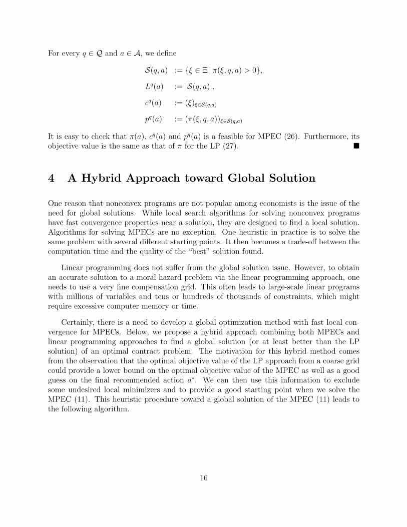
For every q ∈ Q and a ∈ A, we define

S(q, a) := {ξ ∈ Ξ |π(ξ, q, a) > 0},Lq(a) := |S(q, a)|,cq(a) := (ξ)ξ∈S(q,a)

pq(a) := (π(ξ, q, a))ξ∈S(q,a)

It is easy to check that π(a), cq(a) and pq(a) is a feasible for MPEC (26). Furthermore, itsobjective value is the same as that of π for the LP (27). ¥

4 A Hybrid Approach toward Global Solution

One reason that nonconvex programs are not popular among economists is the issue of theneed for global solutions. While local search algorithms for solving nonconvex programshave fast convergence properties near a solution, they are designed to find a local solution.Algorithms for solving MPECs are no exception. One heuristic in practice is to solve thesame problem with several different starting points. It then becomes a trade-off between thecomputation time and the quality of the “best” solution found.

Linear programming does not suffer from the global solution issue. However, to obtainan accurate solution to a moral-hazard problem via the linear programming approach, oneneeds to use a very fine compensation grid. This often leads to large-scale linear programswith millions of variables and tens or hundreds of thousands of constraints, which mightrequire excessive computer memory or time.

Certainly, there is a need to develop a global optimization method with fast local con-vergence for MPECs. Below, we propose a hybrid approach combining both MPECs andlinear programming approaches to find a global solution (or at least better than the LPsolution) of an optimal contract problem. The motivation for this hybrid method comesfrom the observation that the optimal objective value of the LP approach from a coarse gridcould provide a lower bound on the optimal objective value of the MPEC as well as a goodguess on the final recommended action a∗. We can then use this information to excludesome undesired local minimizers and to provide a good starting point when we solve theMPEC (11). This heuristic procedure toward a global solution of the MPEC (11) leads tothe following algorithm.

16

A hybrid method for the optimal contract problem as MPEC (11)

Step 0: Construct a coarse grid Ξ over the compensation interval.Step 1: Solve the LP (27) for the given grid Ξ.

Step 2:

(2.1) : Compute p(a) =∑

ξ∈Ξ

∑q∈Q

π(ξ, q, a), ∀ a ∈ A;

(2.2) : Compute IE[ξ(q)] =∑

ξ∈Ξ

ξπ(ξ, q, a), ∀ q ∈ Q;

(2.3) : Set initial point c0 = (IE[ξ(q)])q∈Q and δ0 = (p(a))a∈A;

(2.4) : Solve the MPEC (11) with starting point (c0, δ0).

Step 3: Refine the grid and repeat Step 1 and Step 2.

Remark If the starting point from an LP solution is close to the optimal solution of theMPEC (11), then the sequence of iterates generated by an SQP algorithm converges Q-quadratically to the optimal solution. See Proposition 2 in Fletcher et al. [4].

One can also develop similar procedures to find global solutions for optimal contractproblems with action and/or compensation lotteries. However, the MPECs for contractswith lotteries are much more numerically challenging problems than the MPEC (11) fordeterministic contracts.

5 An Example and Numerical Results

To illustrate the use of the mixed-integer nonlinear program (7), the MPEC (11) and thehybrid approaches, and to understand the effect of discretizing the set of compensationsC, we only consider problems of deterministic contracts without lotteries. We consider atwo-outcome example in Karaivanov [9]. Before starting the computational work, we sum-marize in Table 1 the problem characteristics of various approaches to computing the optimaldeterministic contracts.

17

Table 1: Problem characteristics of various approaches.MINLP (7) MPEC (11) LP (27)

Regular Variables N N + M |Ξ| ∗N ∗M

Binary Variables M – –Constraints M + 2 2 M ∗ (N + M − 1) + 2Complementarity Const. – M –

Example 1: No Action and Compensation Lotteries

Assume the principal is risk neutral with utility w(q− c(q)) = q− c(q), and the agent is riskaverse with utility

u(c(q), a) =c1−γ

1− γ+ κ

(1− a)1−δ

1− δ.

Suppose there are only two possible outcomes, e.g., a coin-flip. If the desirable outcome (highsale quantities or high production quantities) happens, then the principal receives qH = $3;otherwise, he receives qL = $1. For simplicity, we assume that the set of actions A consistsof M equally-spaced effort levels within the closed interval [0.01, 0.99]. The productiontechnology for the high outcome is described by p(q = qH |a) = aα with 0 < α < 1. Notethat since 0 and 1 are excluded from the action set A, the full-support assumption onproduction technology is satisfied.

The parameter values for the particular instance we solve are given in Table 2.

Table 2: The value of parameters used in Example 1.γ κ δ α U∗ M

0.5 1 0.5 0.7 1 10

We solve this problem first as a mixed-integer nonlinear program (7) and then as anMPEC (11). For the LP lotteries approach, we start with 20 grid points in the compensationgrid (we evenly discretize the compensation set C into 19 segments) and then increase thesize of the compensation grid to 50, 100, 200, . . . , 5000.

We submitted the corresponding AMPL programs to the NEOS server [14]. The mixed-integer nonlinear programs were solved using the MINLP solver [3] on the computer hostnewton.mcs.anl.gov. To obtain fair comparisons between the LP, MPEC, and hybridapproaches, we chose SNOPT [5] to solve the associated mathematical programs. The AMPLprograms were solved on the computer host tate.iems.northwestern.edu.

Table 3 gives the solutions returned by the MINLP solver to the mixed-integer nonlinearprogram (7). We use y = 0 and y = eM as starting points. In both cases, the MINLP solverreturns a solution very quickly. However, it is not guaranteed to find a global solution.

18

Table 3: Solutions of the MINLP approach.Starting Regular Binary Constraints Solve Time ObjectivePoint Variables Variables (in sec.) Valuey = 0 2 10 12 0.01 1.864854251y = eM 2 10 12 0.00 1.877265189

For solving the MPEC (11), we try two different starting points to illustrate the possi-bility of finding only a local solution. The MPEC solutions are given in Table 4 below.

Table 4: Solutions of the MPEC approach with two different starting points.(22 variables and 10 complementarity constraints)

Starting Read Time Solve Time # of Major ObjectivePoint (in sec.) (in sec.) Iterations Valueδ = 0 0 0.07 45 1.079621424δ = eM 0 0.18 126 1.421561553

The solutions for the LP lottery approach with different compensation grids are givenin Table 5. Notice that the solve time increases faster than the size of the grid when |Ξ| isof order 105 and higher, while the number of major iterations only increases about 3 timeswhen we increase the grid size 250 times (from |Ξ| = 20 to |Ξ| = 5000).

Table 5: Solutions of the LP approach with 8 different compensation grids.# of Read Time Solve Time # of Objective

|Ξ| Variables (in sec.) (in sec.) Iterations Value20 400 0.01 0.03 31 1.87608581950 1000 0.02 0.06 46 1.877252488

100 2000 0.04 0.15 53 1.877252488200 4000 0.08 0.31 62 1.877254211500 10000 0.21 0.73 68 1.877263962

1000 20000 0.40 2.14 81 1.8772621842000 40000 0.83 3.53 71 1.8772604605000 100000 2.19 11.87 101 1.877262793

Finally, for the hybrid approach, we first use the LP solution from a compensation gridwith |Ξ| = 20 to construct a starting point for the MPEC (11). As one can see in Table6, with a good starting point, it takes SNOPT only 0.01 seconds to find a solution to theexample formulated as the MPEC (11). Furthermore, the optimal objective value is higherthan that of the LP solution from a fine compensation grid with |Ξ| = 5000.

19

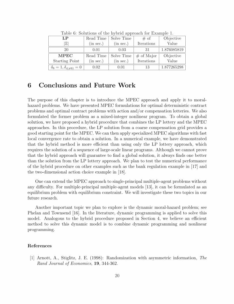
Table 6: Solutions of the hybrid approach for Example 1.LP Read Time Solve Time # of Objective|Ξ| (in sec.) (in sec.) Iterations Value20 0.01 0.03 31 1.876085819

MPEC Read Time Solve Time # of Major ObjectiveStarting Point (in sec.) (in sec.) Iterations Value

δ6 = 1, δi(6=6) = 0 0.02 0.01 13 1.877265298

6 Conclusions and Future Work

The purpose of this chapter is to introduce the MPEC approach and apply it to moral-hazard problems. We have presented MPEC formulations for optimal deterministic contractproblems and optimal contract problems with action and/or compensation lotteries. We alsoformulated the former problem as a mixed-integer nonlinear program. To obtain a globalsolution, we have proposed a hybrid procedure that combines the LP lottery and the MPECapproaches. In this procedure, the LP solution from a coarse compensation grid provides agood starting point for the MPEC. We can then apply specialized MPEC algorithms with fastlocal convergence rate to obtain a solution. In a numerical example, we have demonstratedthat the hybrid method is more efficient than using only the LP lottery approach, whichrequires the solution of a sequence of large-scale linear programs. Although we cannot provethat the hybrid approach will guarantee to find a global solution, it always finds one betterthan the solution from the LP lottery approach. We plan to test the numerical performanceof the hybrid procedure on other examples such as the bank regulation example in [17] andthe two-dimensional action choice example in [18].

One can extend the MPEC approach to single-principal multiple-agent problems withoutany difficulty. For multiple-principal multiple-agent models [13], it can be formulated as anequilibrium problem with equilibrium constraint. We will investigate these two topics in ourfuture research.

Another important topic we plan to explore is the dynamic moral-hazard problem; seePhelan and Townsend [16]. In the literature, dynamic programming is applied to solve thismodel. Analogous to the hybrid procedure proposed in Section 4, we believe an efficientmethod to solve this dynamic model is to combine dynamic programming and nonlinearprogramming.

References

[1] Arnott, A., Stiglitz, J. E. (1998): Randomization with asymmetric information, TheRand Journal of Economics, 19, 344-362.

20

[2] Facchinei, F., Pang, J.-S. (2003): Finite-Dimensional Variational Inequalities and Com-plementarity Problems, Springer Verlag, New York.

[3] Fletcher, R., Leyffer, S. (1999): User manual for MINLP BB, Department of Mathe-matics, University of Dundee, UK.

[4] Fletcher, R., Leyffer, S., Ralph, D., Scholtes, S. (2002): Local convergence of SQPmethods for mathematical programs with equilibrium constraints. Numerical AnalysisReport NA/209, Department of Mathematics, University of Dundee, UK.

[5] Gill, P.E., Murray, W., Saunders, M.A. (2002): SNOPT: An SQP algorithm for large-scale constrained optimization, SIAM Journal on Optimization, 12, 979–1006.

[6] Grossman, S.J., Hart, O.D (1983): An analysis of the principal-agent problem, Econo-metrica, 51, 7–46.

[7] Hart, O.D, Holmstrom, B. (1987): The theory of contracts, in (Bewley, T. eds.) Ad-vances in Economic Theory: Fifth World Congress, 7–46, Cambridge University Press,Cambridge, UK.

[8] Jewitt, I. (1988): Justifying the first-order approach to principal-agent problems, Econo-metrica, 56, 1177–1190.

[9] Karaivanov, A. K. (2001): Computing moral hazard programs with lotteries UsingMatlab, Working paper, Department of Economics, University of Chicago.

[10] Luo, Z.-Q., Pang, J.-S., Ralph, D. (1996): Mathematical Programs with EquilibriumConstraints, Cambridge University Press, Cambridge, UK.

[11] Mirrlees, J. A. (1975): The theory of moral-hazard and unobservable behavior: part I,Mimeo, Nuffield College, Oxford University, Oxford, UK.

[12] Mirrlees, J. A. (1999): The theory of moral-hazard and unobservable behavior: part I,Review of Economic Studies,

[13] Myerson, R. B. (1982): Optimal coordination mechanisms in generalized principal-agentproblems, Journal of Mathematical Economics, 10, 67–81.

[14] The NEOS server for optimization, Webpage: www-neos.mcs.anl.gov/neos/

[15] Outrata, J., Kocvara, M., Zowe, J. (1998): Nonsmooth Approach to OptimizationProblems with Equilibrium Constraints: Theory, Applications, and Numerical Results,Kluwer Academic Publishers, Dordrecht, The Netherlands.

[16] Phelan, C., Townsend, R. M. (1991): Computing multi-period, information-constrainedoptima, The Review of Economic Studies, 58, 853–881.

[17] Prescott, E. S. (1999): A primer on moral-hazard models, Federal Reserve Bank ofRichmond Quarterly Review, 85, 47–77.

21

[18] Prescott, E. S. (2004): Computing solutions to moral-hazard programs using theDantzig–Wolfe decomposition algorithm, Journal of Economic Dynamics and Control,28, 777–800.

[19] Rogerson, W. P. (1985): The first-order approach to principal-agent problems, Econo-metrica, 53, 1357–1368.

[20] Sahinidis, N. V., Tawarmalani, M. (2004): BARON 7.2: Global Opti-mization of Mixed-Integer Nonlinear Programs, User’s Manual, Available athttp://www.gams.com/dd/docs/solvers/baron.pdf.

[21] Scheel, H., Scholtes, S. (2000): Mathematical programs with equilibrium constraints:stationarity, optimality, and sensitivity, Mathematics of Operations Research, 25, 1–22.

[22] Su, C.-L. (2004): A sequential NCP algorithm for solving equilibrium problems withequilibrium constraints, Working paper, Department of Management Science and Engi-neering, Stanford University.

[23] Townsend, R. M. (1987): Economic organization with limited communication, AmericanEconomic Review, 77, 954–971.

[24] Townsend, R. M. (1988): Information constrained insurance: the revelation principleextended, Journal of Monetary Economics, 21, 411–450.

22