1

COMPOSITIONAL MODELS FOR MORTALITY BY AGE,SEX AND CAUSE

Joshua A Salomon

Christopher JL Murray

GPE Discussion Paper Series: No. 11

EIP/GPE/EBD

2

1 Introduction

Reliable information on deaths by cause is an essential input for planning, managing andmonitoring the performance of the health sector in all countries. Detailed estimates ofmortality patterns disaggregated by age and sex for over 100 specific causes have beenpublished at the global and regional level (Murray and Lopez 1996, 1997) as well as at thenational or sub-national level for a number of different countries (Bowie et al 1997, Conchaet al 1996, Lozano et al 1995, Mathers et al. 1999, Murray et al. 1997, 1998, Ruwaardand Kramers 1998). A range of different data sources have been exploited for theestimation of mortality by cause, including vital registration systems, sample registrationsystems, and epidemiological estimates. Where these information sources are not available,however, indirect techniques for estimating cause-of-death patterns can be useful.

For the Global Burden of Disease Study 2000, a number of different health indicators willbe calculated for every country, including mortality by age, sex and cause and measures ofdisease burden such as Disability-Adjusted Life Years (DALYs), which require cause-of-death data as inputs. As a critical step in this exercise, an extensive effort has been launchedto compile all existing data sources on mortality by cause in as many countries as possible,and WHO continues to augment and refine its comprehensive mortality database. Anestimated 17 million deaths, or around thirty percent of all deaths, are currently covered byregistration systems. Inevitably, large gaps remain, particularly in high-mortality areas. Inorder to address these information gaps, models for estimating broad cause-of-deathpatterns can serve as the starting point for indirect methods of estimating attributablemortality for a comprehensive list of detailed causes.

In this paper we describe the development of new models for estimating broad patterns ofmortality by age and sex in areas without adequate death registration data. In the followingsections, we review previous work on developing cause-of-death models, including theGlobal Burden of Disease 1990 study, describe the development of new statistical modelsfor cause-of-death data, present one application of these models based on regional variationin cause-of-death patterns, and discuss further directions for research in this area.

2 Background

Indirect methods for estimating cause-of-death structure were first developed by Preston(1976), who modeled the relationship between total mortality and cause-specific mortalityfor twelve broad groups of causes using historical vital registration data for industrializedcountries and a few developing countries. In particular, cause-specific mortality waspostulated to be a linear function of total mortality. Preston’s work has formed the basis ofnearly all subsequent approaches to estimating cause-of-death patterns in regions withoutvital registration. Typically, these refinements have involved estimating equations for specificage groups, incorporating more recent data or examining more detailed causes (Bulutao1993, Hakulinen et al.1986, Hull et al. 1981, Lopez and Hull 1983, Murray et al. 1992).

For the GBD 1990 study (Murray and Lopez 1996), cause of death models were used toestimate mortality in three broad clusters of causes as a function of mortality from all causes. The three cause clusters were: Group I, consisting of communicable diseases, maternalcauses, conditions arising in the perinatal period, and nutritional deficiencies; Group II,

3

encompassing the noncommunicable diseases; and Group III, comprising all injuries,whether intentional or unintentional. The data set used in this study consisted ofobservations on recent mortality patterns from 67 countries plus older data sets from the 36countries with reliable data available before 1965. Separate regressions were run for eachcause group, and each of fourteen age-sex groups, using the following form:

iii TM εββ ++= lnln 10 (1)

where iM is the mortality rate from the specified cause group in observation i, iT is themortality rate from all causes combined, 0β and 1β are coefficients to be estimated, and iεis an observation-specific error term drawn from a normal distribution with mean 0 andunknown variance to be estimated. In this framework, the mortality rates from Groups I, IIand III in a given country and year are assumed to be realizations of three independentnormally distributed random processes. The regression results from this model suggested astrong association between the level of all-cause mortality and the level of Group II mortalityand between all-cause mortality and Group I mortality in all but the oldest age groups. Thepredictive power of all-cause mortality for Group III mortality was relatively weak, on theother hand.

Based on the regression results, Monte Carlo simulation methods were applied in order todevelop estimates of the probability distribution of predicted mortality rates for each causegroup conditional on some fixed value for all-cause mortality. These results were then usedto examine patterns of deviation from the predicted distribution of deaths among the threelarge cause groups.

An important limitation of the standard regression approach used in the GBD 90 exercise isthat it does not recognize two fundamental features of cause-of-death data. Because cause-of-death patterns represent the proportions of all deaths that are attributed to each of a setof mutually exclusive and collectively exhaustive causes or cause groups, this type of datahas two basic constraints common to all types of compositional data: (i) the proportion ofdeaths attributed to each cause must be between 0 and 1; and (ii) the set of proportions forall of the cause groups must sum to one. In the regression model described above,violations of both constraints are possible. For example, it would be possible for predictedmortality for one cause group in this model to exceed the all-cause mortality rate, thusviolating the first constraint. Moreover, because independent regressions are run on each ofthe three cause groups for the same country-year observation, they are not constrained tosum to the all-cause mortality rate, which violates the second constraint. In the GBD 90, anadditional normalization step was undertaken after the predicted mortality rates werecomputed in order to impose the second constraint, but the model itself does not takeaccount of the interdependence of the three groups that constitute total mortality.

An alternative to the use of independent regression models for each constituent cause groupis offered by a class of general statistical models described as compositional models, withapplications from a range of disciplines, including political science, geology and biologyamong others. This paper describes the adaptation of the statistical methods forcompositional models to the problem of predicting cause-of-death patterns.

4

3 Methods

3.1 Statistical model

A general statistical model for compositional data has been presented by Katz and King(1999) in an application to multiparty electoral data. The description below uses the samenotation as the Katz and King model.

In order to model compositional data with J different cause groups, we first define a vectorof cause fractions: ),...,( 1 iJii PPP = for each observation i. Following Aitchison (1986), thedata is modeled using the additive logistic normal distribution. First, a (J-1) vector iY isgenerated by calculating the log ratios of each cause fraction relative to the fraction for causeJ:

=

iJ

ijij P

PY ln (2)

The vector ),...,( )1(1 −= Jiii YYY is assumed to be multivariate normal with mean vector µ andvariance matrix Σ. The expectation of each log-ratio is assumed to be a linear function ofthe explanatory variables in the model:

jijij X βµ = (3)

where ijX is a vector of explanatory variables and jβ are parameters to be estimated.

3.2 Data

The dataset consists of mortality data from 58 different countries from the years 1950 to1998. The series vary in terms of length; in total there are 1,613 country-years ofobservation. Table 1 lists the countries in the dataset and the range of years for each series.As in the previous exercise, separate models were estimated for each sex and age group. The complete dataset may therefore be considered as 20 separate datasets divided by sexand the following age groups: <1 month, 1-11 months, 1-4 years, 5-9 years, 10-14 years,and so on by five-year age groups, up to 80-84 years and 85 years and older. For the twoyoungest age groups, a smaller number of observations were available because a number ofcountries over different periods reported only on the age range from birth to 11 months. Atotal of 586 country-years of observations were available for the first two age groups.

3.3 Model-fitting

In addition to revising the statistical model used in the previous study, we have alsoconsidered additional covariates beyond all-cause mortality. The objective was to identifyvariables that would be likely to have a strong relationship to cause-specific mortality, butalso variables for which estimates would be available in all countries, since one of the goalsof the exercise is to use the model to predict broad patterns of mortality for countrieswithout vital registration data. The variables that were selected based on these criteria wereall-cause mortality, as before, plus income per capita in international dollars. Both variableswere included in logged form as this formulation tended to provide a better fit than the linear

5

one. In the results below, we report on two different model formulations, one with only all-cause mortality; and one with both all-cause mortality and income per capita.

Given the model specification described here, the multivariate normal model for the logratios may be written as a system of two regression equations. For the model that includesall-cause mortality and income per capita, the system of equations are as follows:

12101 )ln()ln( iiii XTY εβββ +++= (4a)

22102 )ln()ln( iiii XTY εγγγ +++= (4b)

where 1iY and 2iY are the log-ratios as defined in Equation (2), iT is the all-cause mortalityrate, and iX is income per capita .The two residual terms 1iε and 2iε have expectations of0, variances of 1σ and 2σ , respectively, and correlation of ρ.

Maximum likelihood estimates of the coefficients, the variance-covariance matrix for theseestimators, and the variance-covariance matrix for the residuals, have been obtained usingthe seemingly unrelated regression model (Greene 1993). Seemingly unrelated regression isallowed when both equations have identical explanatory variables. The seemingly unrelatedregression model produces the same coefficient estimates as equation-by-equation OLSregression but accounts for correlations in the error terms and the full covariance structure ofthe coefficients.

4 Results

The first set of regressions that were run included only all-cause mortality as an explanatoryvariable. The relationship between the total level of mortality and cause-specific mortalitywas one of the key points of interest in the original Preston models. The notion of theepidemiological transition suggests that as total mortality declines, the relative importance ofthe communicable diseases (Group I) tends to decrease compared to other causes. Thefirst set of regression models allows an empirical examination of the epidemiologicaltransition by age and sex. Using the estimated coefficients from the regression results,predicted values for Y1 and Y2 were computed for each observation in the data set based onthe level of all-cause mortality. These predictions were then transformed into proportions bycause group using the multivariate logistic transformation:

∑−

=

+=

1

1

)exp(1

)exp(J

jj

jj

Y

YP (5)

with P3 calculated as 1 – P1 – P2.

The results are plotted by age and sex in Figure 1 as a series of ternary diagrams, each ofwhich represents in two dimensions a range of different distributions of death across thethree cause groups. The first four rows of diagrams are for males, and the second set forfemales. Each diagram shows the results for one age group, ordered from left to right byrow, from ages 0 to 1 month in the top left to ages 85 years and older in the bottom right

6

corner of each four-row block. In each ternary diagram, one predicted distribution of deathsappears as one point on the graph. The fraction of deaths due to each cause is representedas the perpendicular distance from the side of the triangle opposite the labeled vertex. Thenearer a dot is to the vertex, the higher the proportion due to that cause. On the diagram thevertices are labeled as G1 at the top, G2 at the bottom right and G3 at the bottom leftindicating Groups I, II and III, respectively. Thus, each diagram represents, for one age andsex group, the predicted distributions of deaths from Groups I, II and III at different levelsof total mortality. For example, a point located near the top vertex would have a very highproportion of Group I deaths and low proportions for Groups II and III. A point locatedalong the right side of the triangle would have no Group III deaths.

The epidemiological transition may be viewed in each diagram as the path traced by thepoints as total mortality declines. In children, this movement is from the top of the diagramtowards the bottom, in other words, a movement away from Group I causes. For youngadult age groups in males, depicted in the second and third rows, the transition moves fromleft to right, which indicates an increase in Group II relative to Group III as mortalitydecreases. Interestingly, for young adult females, the transition moves first from Group I toGroup II as maternal conditions decline as important causes of death, but then from GroupII to Group III as both infectious and chronic causes of death decline, but injuries maintainrelatively stable levels. At the oldest age groups in both sexes, there is little evidence of theepidemiological transition, as Group II conditions dominate at all levels of mortalityrepresented in the data set.

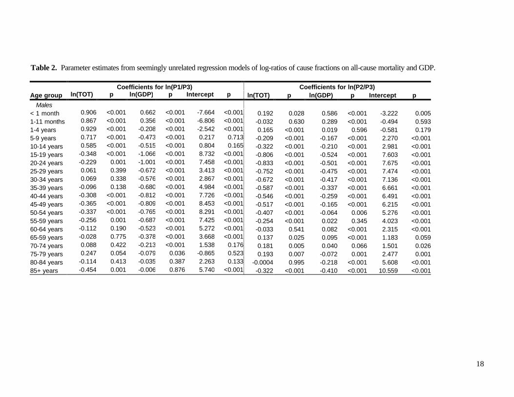
The second set of regression models included income per capita as an explanatory variablein addition to all-cause mortality. Table 2 summarizes the regression results for each ageand sex group. In most models, the coefficients on both income and total mortality arehighly significant.

In nearly all cases, increases in income per capita are associated with declines in both GroupI and Group II as proportions of all causes of death relative to Group III causes. Themagnitude of these relative declines tends to be larger for Group I than for Group II, whichsuggests that Group II causes increase relative to Group I causes as income rises.

The relationship between cause-of-death patterns and all-cause mortality levels, conditionalon income level, is somewhat more complicated but confirms the general patternsdemonstrated in the model with only total mortality. For males, lower mortality levels areaccompanied by an increase in the importance of Group II causes relative to Group IIIcauses in most age groups. For Group I this relationship varies according to age. Forfemales, on the other hand, both Group I and Group II tend to decrease in importancerelative to Group III as mortality declines.

While the signs and relative magnitudes of the parameter estimates from the regressionmodel offer some insights into the relationships of interest, the most important quantities ofinterest are the actual predictions of cause-of-death patterns, which are nonlinear functionsof these parameters. More precisely, we are interested in the probability distributions of thepredicted cause-of-death components given a particular set of values for all-cause mortalityand GDP per capita. In order to derive these distributions, we have used Monte Carlosimulation techniques according to the following steps.

In each of 5000 iterations, we have taken a random draw from a multivariate normaldistribution around the estimators, with a mean vector consisting of the maximum likelihood

7

estimates of the β and γ coefficients and the variance-covariance matrix derived from theregression results. We have then computed the expected values for the log-ratios µ1 and µ2

using specified values for T and X and taken a random draw of Y1 and Y2 from a bivariatenormal distribution with mean vector µ = {µ1, µ2} and variance matrix constructed from theregression estimates of σ1, σ2 and ρ. We have used these sampled values of Y1 and Y2 tocompute P1 and P2 using the multivariate logistic transformation in equation (5). As before,P3 was calculated for each draw as 1 – P1 – P2. Thus, in generating 5000 simulations of thecause-of-death vector P, it is possible to summarize the probability distribution for thepredicted contributions of the three cause groups given values of T and X. The results fromthis approach are quite useful in estimating cause of death patterns for residual areas incountries where only part of the population is covered by vital registration, and in definingregional cause-of-death patterns as described below.

5 Applications

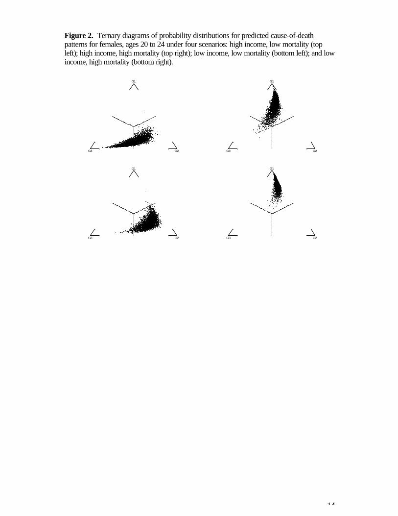
To illustrate the simulation approach from Section 4, we consider one age group as anexample. Using the steps described above for females ages 20 to 24 years, we havegenerated 5000 different simulated cause-of-death patterns for each of 4 different scenariosrepresenting high and low values for total mortality and income per capita. We haveexamined all-cause mortality at levels of 50 and 500 per 100,000, and income per capita atlevels of 2000 and 12,000 per person. Figure 2 shows the results of these simulations. Thetop left graph shows the distribution under high income and low mortality; the top right graphshows the high income, high mortality scenario; the bottom left graph show low income, lowmortality; and the bottom right graph low income, high mortality. These figures are ternarydiagrams, which represent the three different proportions in two dimensions as describedabove. Each simulated cause-of-death pattern appears as one point on the graph. Asbefore, the vertices labeled as G1, G2 and G3 indicate Groups I, II and III; the nearer a dotis to a vertex, the higher the proportion from that cause group.

The top left figure indicates that at high income and low mortality, Group I represents arelatively small proportion of deaths in this age group, Group II represents a relatively largeproportion, and there is a wide range of variability in terms of the proportion due to GroupIII. The bottom right figure, on the other hand, shows that at low income and high mortality,Group I dominates, while Group II and especially Group III make up only smallcomponents of total mortality. Examining the off-diagonal graphs, we can also look at theindependent effects of changes in income alone or changes in all-cause mortality alone. Thus, moving from the left column to the right column represents a change from lowmortality to high mortality while holding the level of income constant (at a high level in the toprow or a low level in the bottom row). In both cases, a shift to high mortality isaccompanied by a shift away from Groups II and III towards Group I. Movements fromthe top row to the bottom row, meanwhile, represent changes from high income to lowincome holding the level of all-cause mortality constant. Here, the major shift is from widelyvariable and relatively high Group III contributions to more concentrated and lower ones.

As in the GBD 90, one of the useful applications of cause-of-death models is to examinepatterns of deviation from the expected cause composition across countries or regions,based on the probability distribution for a predicted cause-of-death pattern. Graphically, thiswould be equivalent to examining where an observed cause-of-death pattern would fallwithin the distribution of points on one of the diagrams in Figure 2; i.e., how does the

8

observed pattern compare to the pattern that would be predicted conditional on the levels ofall-cause mortality and income per capita associated with that observation.

Given some assumptions about the stability of this pattern of deviation over short timeintervals within a country or across countries in the same mortality stratum, it is possible touse the observed cause of death pattern in a reference population to estimate the cause ofdeath pattern for some other population while taking into account differences in theexplanatory variables. Some examples of applications would be:

• estimating the cause-of-death pattern in non-registration areas for a country in whichpart of the population is covered by the vital registration system

• forecasting the cause-of-death pattern for a country where the last vital registrationdata was available several years in the past

• estimating the cause-of-death pattern for a country where information is available forother countries in the same region.

All of these applications are based on the assumption that patterns of deviation from thecause compositions predicted by the model will have some stability across time and place;for example, we hypothesize that if young adults in Canada tend to have a low proportion ofGroup I deaths and a high proportion of Group II deaths in one year given the levels of all-cause mortality and income in that year, that the next year’s composition will be similarly lowin Group I and high in Group II given that year’s total income and mortality. This hypothesisbuilds on the notion that all-cause mortality and income per capita explain only some of thevariation in cause-of-death patterns, while the other sources of this variation are unmeasuredbut assumed to be relatively stable. In other words, the cause-of-death pattern in Canadadiffers from that which we would predict based only on total mortality and income becausethere are other factors which influence the pattern; we assume that these other factors willchange gradually over time, which would imply that the deviation from the prediction shouldalso move gradually.

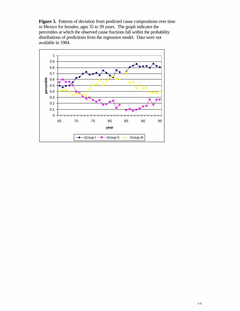
Figure 3 gives one example that suggests that the hypothesis of stability over time isreasonable over short time intervals. The figure illustrates the pattern of deviation frompredicted cause compositions over time in Mexico for females ages 35 to 39 years. Eachline shows, for one cause group over time, the percentile at which the observed proportionfalls in the probability distribution of predicted fractions given Mexico’s income per capitaand total mortality for females 35 to 39 in that year. The figure demonstrates that the patternof deviation may change considerably over long periods such as 30 years but that, in ashorter period of up to five years, the shift is a rather smooth and gradual one. In otherwords, if we were to assume stability over time and use the pattern of deviation from 1990to predict the cause composition in 1995 given levels of income and total mortality, theestimated cause-of-death pattern in 1995 would match the observed pattern reasonablywell.

We may also examine the hypothesis that patterns of deviation from one country may beused to predict cause-of-death patterns in another country in the same demographic region. The logic behind this hypothesis is similar to the logic around stability over time: we assumethat deviation from predicted patterns is due to variability in factors other than total mortalityand income that influence cause-of-death patterns. We assume further that some of thesefactors will be similar in countries that are close to each other either geographically or interms of demographic trends.

9

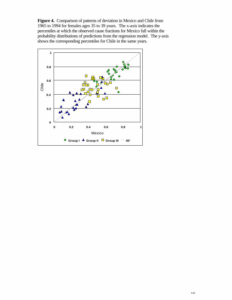
In Figure 4, data from Chile is plotted against the Mexican data, for females ages 35 to 39years for the years 1965 to 1994. The horizontal axis indicates the percentiles at which theobserved cause fractions for Mexico fall in the probability distribution of predicted fractions,as above. The vertical axis indicates the corresponding percentiles for Chile in the sameyears, in reference to the predicted fractions conditional on Chile’s mortality and incomelevels in those years. There is a very strong relationship between the two patterns ofdeviation, although there is some scatter around the 45° line, which is explained in part bymeasurement error around the mortality data from which the observed fractions are derived. Overall, this example suggests that deviation patterns may be quite similar within groups ofsimilar countries, which would allow predictions of cause-of-death patterns in countrieswhere registration data is not available but for which neighboring countries do have data.

6 CodMod

The applications described above have been formalized in a simple spreadsheet programcalled CodMod. The program uses Monte Carlo simulation methods to generateprobability distributions around predicted cause-of-death patterns conditional on values forall-cause mortality and income per capita. CodMod incorporates the regression modelsdescribed in this paper and allows two main operations:

• analysis of deviation in observed cause-of-death patterns given levels of mortaltiyand income

• predictions of cause-of-death patterns conditional on a reference pattern ofdeviation and levels of mortality and income.

In the first operation, the user simply inputs an observed set of cause fractions, mortalitylevel and income per capita level for one or more different age-sex groups, and CodModproduces the probability distribution for the predicted cause patterns at that level of mortalityand income and compares the observed pattern to this predicted distribution. Thecomparison is reported in terms of the percentiles at which each cause fraction falls in thepredicted distribution, as well as the number of standard deviations between each of theobserved fractions and the expected fractions.

In the second operation, the user inputs a reference pattern of deviation for one or moreage-sex groups in terms of percentiles at which cause fractions should fall, as well as levelsof mortality and income. The outputs then include both the expected cause of death patternat the specified levels of income and mortality as well as the estimated pattern given thespecified level of deviation.

Thus, for example, if the vital registration system covers only one region in a country,CodMod may be used to examine the pattern of deviation in that region from the predictedcause-of-death pattern at the local levels of income and total mortality. If it is assumed thata similar pattern of deviation would hold in the non-registration areas of the country, theninformation on total mortality levels and income in the non-registration areas could be usedto predict the cause-of-death patterns in these areas.

For the World Health Report 2000, CodMod was used to develop regional patterns ofdeviation from predicted cause compositions, which were then used to estimate mortality bybroad causes for countries in which no registration data were available.

10

7 Conclusions

In this paper we have described recent work on developing models to predict broad cause-of-death patterns based on information about the total level of mortality by age and sex andincome per capita. This work builds upon previous efforts to model the relationshipbetween the level of mortality from all causes and the fractions of deaths attributable tospecific causes.

One of the new features of the models described in this paper is their use of data on incomeper capita across countries and over time, which was demonstrated to be a powerfulexplanatory variable in understanding patterns of mortality by cause. As time series of GDPper capita estimates are now available for a wide range of countries, this source ofinformation provides important advantages for modeling variation in cause-of-death patterns. As work on cause-of-death models proceeds, it will be important to explore other variablethat might offer similar advantages.

The statistical basis for cause-of-death models has also been enhanced by the adaptation ofmodels for compositional data that were previously developed in other areas. These modelstake account of the key features of this type of data, namely that the fraction of deathsattributable to each cause is bounded by zero and one, and that all of the fractions must sumto unity. Further innovations may be possible in future iterations of this work, includingdevelopment of compositional models designed specifically for panel data.

Perhaps most importantly, the latest round of cause-of-death models described hereincorporates a more extensive database on mortality by age, sex and cause than in previousefforts. Increasing the range of observed cause-of-death patterns will improve the validity ofextrapolations from the countries with registration systems to data-poor settings. Anextensive effort is underway at WHO to develop the most comprehensive database ofmortality information from vital registration systems, sample registration systems andpopulation laboratories. As this body of information grows, the predictive power of cause-of-death models will continue to increase.

Current estimates indicate that around thirty percent of all deaths worldwide are covered byvital registration systems. While this data provides a unique source of information for publichealth monitoring, greater efforts need to be made to improve coverage in developingpopulations, particularly where mortality is high. The public health utility of these data go wellbeyond targeting priorities such as vaccination, diarrhoeal disease control and containing theHIV epidemic, and WHO is strengthening efforts with countries to promote interim solutionssuch as sentinel surveillance systems which yield plausible and useful information on cause-of-death patterns without requiring full registration. In the meantime, cause-of-death modelsprovide a valuable tool for estimating broad patterns of mortality by age, sex and cause, andcontinued progress in this research area is anticipated.

11

8 References

Aitcheson J (1986). The statistical analysis of compositional data. New York, JohnWiley.

Bowie C, Beck S, Bevan G, Raftery J, Silvertion F, and Stevens J (1997). Estimating theburden of disease in an English region. Journal of Public Health Medicine, 19:87-92.

Bulutao R (1993) Mortality by cause, 1970 to 2015. In: Gribble JN, Preston SH, eds. Theepidemiological transition. Policy and planning implications for developingcountries (Workshop proceedings). Washington, DC, National Academy Press.

Concha M, Aguilera, X, Albala C, et al (1996). Estudio ecarga de enfermedad informefinal. Estudio Prioridades de Inversio en Salud. Bogotá, Minsterio de Salud.

Greene WH (1993). Econometric analysis. New York, Macmillan Publishing Company.

Hakulinen T et al. (1986) Global and regional mortality patterns by cause of death in 1980. International journal of epidemiology, 15: 226-233.

Hull TH et al. (1981) A framework for estimating causes of death in Indonesia. Majalahdemografi Indonesia, 15: 77-125.

Katz J, King G (1999). A statistical model for multiparty electoral data. AmericanPolitical Science Review, 93(1): 15-32.

Lopez AD, Hull TH (1983) A note on estimating the cause of death structure in highmortality populations. Population bulletin of the United Nations, 14: 66-70.

Lozano R, Murray CJL, Frenk J, and Bobadilla J (1995). Burden of Disease Assessmentand Health System Reform: Results of a Study in Mexico. Journal for InternationalDevelopment, 7(3): 555-564.

Mathers C, Vos T, Stevenson C (1999). The burden of disease and injury in Australia.Australian Institute of Health and Welfare, Canberra: AIHW

Murray CJL, Lopez, AD, eds (1996). The global burden of disease: a comprehensiveassessment of mortality and disability from diseases, injuries and risk factors in1990 and projected to 2020. Cambridge, Harvard University Press (Global Burden ofdisease and Injury Series, Vol. 1).

Murray CJL, and Lopez A (1997). Mortality by cause for eight regions of the world: GlobalBurden of Disease Study. Lancet, 349: 1269-1276.

Murray CJL, Lopez AD (2000). Progress and directions in refining the global burden ofdisease approach: response to Williams. Health Economics 9: 69-82.

Murray CJL. Mahapatra P. Ashley R. Michaud C. George A. Horbon P. Akhavan D. et al.(1997). The Health Sector in Mauritius: Resource Use, Intervention Cost and

12

Options for Efficiency Enhancement. Cambridge, Harvard Center for Population andDevelopment Studies.

Murray CJL. Michaud CM. McKenna MT. and Marks JS (1998). U. S. Patterns ofMortality by County and Race: 1965-1994. Cambridge, Harvard Center forPopulation and Development Studies and Centers for Disease Control.

Murray CJL, Yang G, Qiao X (1992) Adult mortality: levels, patterns and causes. In:Feachem RGS et al., eds. The health of adults in the developing world. Oxford,Oxford University Press, 23-111.

Preston SH (1976) Mortality patterns in national populations. New York, AcademicPress.

Ruwaard D, Kramers PGN (1998). Public health status and forecasts. The Hague,National Institute of Public Health and Environmental Protection.

13

Figure 1. The epidemiological transition. The first four rows of diagrams representsdifferent ages for males, from age 0 to 1 month in the top left corner to ages 85 years andolder in the bottom right. The second block represents different ages for females, in thesame order. Each diagram is a ternary plot that presents mortality fractions by cause as theperpendicular distance to each base of the triangle, with the Group I proportion indicated bydistance to the bottom side, Group II the distance to the left side and Group III the distanceto the right side. The series of points in each diagram represent the predicted causecompositions at different levels of all-cause mortality.

` ' `

' `

G1

' G3 G2

` ' `

' `

G1

' G3 G2

` ' `

' `

G1

' G3 G2

` ' `

' `

G1

' G3 G2

` ' `

' `

G1

' G3 G2

` ' `

' `

G1

' G3 G2

` ' `

' `

G1

' G3 G2

` ' `

' `

G1

' G3 G2

` ' `

' `

G1

' G3 G2

` ' `

' `

G1

' G3 G2

` ' `

' `

G1

' G3 G2

` ' `

' `

G1

' G3 G2

` ' `

' `

G1

' G3 G2

` ' `

' `

G1

' G3 G2

` ' `

' `

G1

' G3 G2

` ' `

' `

G1

' G3 G2

` ' `

' `

G1

' G3 G2

` ' `

' `

G1

' G3 G2

` ' `

' `

G1

' G3 G2

` ' `

' `

G1

' G3 G2

` ' `

' `

G1

' G3 G2

` ' `

' `

G1

' G3 G2

` ' `

' `

G1

' G3 G2

` ' `

' `

G1

' G3 G2

` ' `

' `

G1

' G3 G2

` ' `

' `

G1

' G3 G2

` ' `

' `

G1

' G3 G2

` ' `

' `

G1

' G3 G2

` ' `

' `

G1

' G3 G2

` ' `

' `

G1

' G3 G2

` ' `

' `

G1

' G3 G2

` ' `

' `

G1

' G3 G2

` ' `

' `

G1

' G3 G2

` ' `

' `

G1

' G3 G2

` ' `

' `

G1

' G3 G2

` ' `

' `

G1

' G3 G2

` ' `

' `

G1

' G3 G2

` ' `

' `

G1

' G3 G2

` ' `

' `

G1

' G3 G2

` ' `

' `

G1

' G3 G2

14

Figure 2. Ternary diagrams of probability distributions for predicted cause-of-deathpatterns for females, ages 20 to 24 under four scenarios: high income, low mortality (topleft); high income, high mortality (top right); low income, low mortality (bottom left); and lowincome, high mortality (bottom right).

G1

G3 G2

G1

G3 G2

G1

G3 G2

G1

G3 G2

15

Figure 3. Patterns of deviation from predicted cause compositions over timein Mexico for females, ages 35 to 39 years. The graph indicates thepercentiles at which the observed cause fractions fall within the probabilitydistributions of predictions from the regression model. Data were notavailable in 1984.

0

0.1

0.2

0.3

0.4

0.5

0.6

0.7

0.8

0.9

1

65 70 75 80 85 90 95

year

perc

entil

e

Group I Group II Group III

16

Figure 4. Comparison of patterns of deviation in Mexico and Chile from1965 to 1994 for females ages 35 to 39 years. The x-axis indicates thepercentiles at which the observed cause fractions for Mexico fall within theprobability distributions of predictions from the regression model. The y-axisshows the corresponding percentiles for Chile in the same years.

0 0.2 0.4 0.6 0.8 1

Mexico

0

0.2

0.4

0.6

0.8

1

Chi

le

Group I Group II Group III 45°

17

Table 1. Countries and years in database. First and last years of observaion are indicated,although one or more intervening years may be missing in some cases.

CountryFirstyear Last year Country

Firstyear Last year

Albania 1992 1993 Latvia 1980 1997Argentina 1966 1996 Lithuania 1987 1998Armenia 1990 1997 Luxembourg 1967 1997Australia 1950 1995 Macedonia 1992 1997Austria 1955 1998 Malta 1965 1998Azerbaijan 1987 1997 Mexico 1958 1995Belarus 1987 1997 Netherlands 1950 1997Belgium 1954 1994 New Zealand 1950 1996Bulgaria 1980 1997 Norway 1951 1995Canada 1950 1997 Poland 1970 1996Chile 1955 1994 Portugal 1955 1998Costa Rica 1961 1995 Republic Of Moldova 1992 1996Croatia 1991 1997 Romania 1980 1998Czech Republic 1986 1997 Russian Federation 1989 1997Denmark 1952 1996 Singapore 1963 1997Estonia 1987 1997 Slovak Republic 1992 1995Finland 1952 1996 Slovenia 1992 1997France 1950 1997 Spain 1951 1996Georgia 1981 1990 Sweden 1951 1996Germany 1990 1998 Switzerland 1951 1994Greece 1961 1997 Tajikistan 1986 1992Hungary 1960 1997 Turkmenistan 1987 1994Iceland 1951 1995 Ukraine 1989 1997Ireland 1950 1996 United Kingdom 1950 1997Israel 1975 1996 United States 1950 1997Italy 1951 1996 Uruguay 1955 1990Japan 1950 1997 Uzbekistan 1992 1993Kazakstan 1987 1997 Venezuela 1955 1994Kyrgyzstan 1987 1998 Yugoslavia, Former 1968 1990

18

Table 2. Parameter estimates from seemingly unrelated regression models of log-ratios of cause fractions on all-cause mortality and GDP.

Coefficients for ln(P1/P3) Coefficients for ln(P2/P3)Age group ln(TOT) p ln(GDP) p Intercept p ln(TOT) p ln(GDP) p Intercept p

Males< 1 month 0.906 <0.001 0.662 <0.001 -7.664 <0.001 0.192 0.028 0.586 <0.001 -3.222 0.0051-11 months 0.867 <0.001 0.356 <0.001 -6.806 <0.001 -0.032 0.630 0.289 <0.001 -0.494 0.5931-4 years 0.929 <0.001 -0.208 <0.001 -2.542 <0.001 0.165 <0.001 0.019 0.596 -0.581 0.1795-9 years 0.717 <0.001 -0.473 <0.001 0.217 0.713 -0.209 <0.001 -0.167 <0.001 2.270 <0.00110-14 years 0.585 <0.001 -0.515 <0.001 0.804 0.165 -0.322 <0.001 -0.210 <0.001 2.981 <0.00115-19 years -0.348 <0.001 -1.066 <0.001 8.732 <0.001 -0.806 <0.001 -0.524 <0.001 7.603 <0.00120-24 years -0.229 0.001 -1.001 <0.001 7.458 <0.001 -0.833 <0.001 -0.501 <0.001 7.675 <0.00125-29 years 0.061 0.399 -0.672 <0.001 3.413 <0.001 -0.752 <0.001 -0.475 <0.001 7.474 <0.00130-34 years 0.069 0.338 -0.576 <0.001 2.867 <0.001 -0.672 <0.001 -0.417 <0.001 7.136 <0.00135-39 years -0.096 0.138 -0.680 <0.001 4.984 <0.001 -0.587 <0.001 -0.337 <0.001 6.661 <0.00140-44 years -0.308 <0.001 -0.812 <0.001 7.726 <0.001 -0.546 <0.001 -0.259 <0.001 6.491 <0.00145-49 years -0.365 <0.001 -0.809 <0.001 8.453 <0.001 -0.517 <0.001 -0.165 <0.001 6.215 <0.00150-54 years -0.337 <0.001 -0.765 <0.001 8.291 <0.001 -0.407 <0.001 -0.064 0.006 5.276 <0.00155-59 years -0.256 0.001 -0.687 <0.001 7.425 <0.001 -0.254 <0.001 0.022 0.345 4.023 <0.00160-64 years -0.112 0.190 -0.523 <0.001 5.272 <0.001 -0.033 0.541 0.082 <0.001 2.315 <0.00165-59 years -0.028 0.775 -0.378 <0.001 3.668 <0.001 0.137 0.025 0.095 <0.001 1.183 0.05970-74 years 0.088 0.422 -0.213 <0.001 1.538 0.176 0.181 0.005 0.040 0.066 1.501 0.02675-79 years 0.247 0.054 -0.079 0.036 -0.865 0.523 0.193 0.007 -0.072 0.001 2.477 0.00180-84 years -0.114 0.413 -0.035 0.387 2.263 0.133 -0.0004 0.995 -0.218 <0.001 5.608 <0.00185+ years -0.454 0.001 -0.006 0.876 5.740 <0.001 -0.322 <0.001 -0.410 <0.001 10.559 <0.001

19

Table 2. (continued)

Coefficients for ln(P1/P3) Coefficients for ln(P2/P3)Age group ln(TOT) p ln(GDP) p Intercept p ln(TOT) p ln(GDP) p Intercept p

Females< 1 month 0.949 <0.001 0.732 <0.001 -8.524 <0.001 0.217 0.022 0.643 <0.001 -3.923 0.0011-11 months 0.932 <0.001 0.315 <0.001 -6.680 <0.001 -0.050 0.428 0.254 <0.001 0.047 0.9581-4 years 1.027 <0.001 -0.061 0.106 -3.882 <0.001 0.257 <0.001 0.187 <0.001 -2.216 <0.0015-9 years 1.005 <0.001 -0.341 <0.001 -1.179 0.023 0.044 0.121 -0.036 0.178 0.604 0.05810-14 years 1.129 <0.001 -0.396 <0.001 -1.006 0.054 0.134 <0.001 -0.162 <0.001 1.618 <0.00115-19 years 1.036 <0.001 -0.849 <0.001 2.378 <0.001 -0.009 0.812 -0.562 <0.001 5.204 <0.00120-24 years 1.383 <0.001 -0.738 <0.001 0.051 0.927 0.178 <0.001 -0.526 <0.001 4.278 <0.00125-29 years 1.607 <0.001 -0.422 <0.001 -3.681 <0.001 0.302 <0.001 -0.385 <0.001 2.880 <0.00130-34 years 1.807 <0.001 -0.308 <0.001 -5.978 <0.001 0.366 <0.001 -0.275 <0.001 1.951 <0.00135-39 years 1.719 <0.001 -0.404 <0.001 -5.394 <0.001 0.274 <0.001 -0.244 <0.001 2.383 <0.00140-44 years 1.532 <0.001 -0.505 <0.001 -4.216 <0.001 0.188 <0.001 -0.243 <0.001 3.156 <0.00145-49 years 1.280 <0.001 -0.503 <0.001 -3.471 <0.001 0.105 0.026 -0.225 <0.001 3.743 <0.00150-54 years 1.440 <0.001 -0.360 <0.001 -6.186 <0.001 0.258 <0.001 -0.163 <0.001 2.497 <0.00155-59 years 1.314 <0.001 -0.290 <0.001 -6.336 <0.001 0.295 <0.001 -0.139 <0.001 2.275 <0.00160-64 years 1.484 <0.001 -0.079 0.072 -9.765 <0.001 0.405 <0.001 -0.068 0.002 1.037 0.02965-59 years 1.418 <0.001 -0.0004 0.992 -10.447 <0.001 0.358 <0.001 -0.101 <0.001 1.747 0.00170-74 years 1.129 <0.001 0.041 0.389 -9.016 <0.001 0.128 0.006 -0.188 <0.001 4.338 <0.00175-79 years 0.611 <0.001 -0.016 0.742 -4.446 0.001 -0.320 <0.001 -0.377 <0.001 9.899 <0.00180-84 years -0.140 0.307 -0.168 0.001 3.645 0.021 -0.756 <0.001 -0.573 <0.001 15.844 <0.00185+ years -0.826 <0.001 -0.262 <0.001 11.578 <0.001 -0.912 <0.001 -0.743 <0.001 19.374 <0.001