compositional approach to design of digital...
TRANSCRIPT
School of Electrical and Electronic Engineering
Compositional Approach to
Design of Digital Circuits
Arseniy Alekseyev
Technical Report Series
NCL-EEE-MICRO-TR-2014-191
June 2014

Contact:
Supported by EPSRC grants EP/G037809/1 and EP/K001698/1
NCL-EEE-MICRO-TR-2014-191
Copyright c© 2014 University of Newcastle upon Tyne
School of Electrical and Electronic Engineering,
Merz Court,
University of Newcastle upon Tyne,
Newcastle upon Tyne, NE1 7RU, UK
http://async.org.uk/

University of Newcastle upon Tyne
School of Electrical and Electronic Engineering
Compositional Approach to
Design of Digital Circuits
by Arseniy Alekseyev
PhD Thesis
June 2013
Contents
1 Introduction 1
1.1 Contributions . . . . . . . . . . . . . . . . . . . . . . . . . . . . . . . 4
1.2 Overview . . . . . . . . . . . . . . . . . . . . . . . . . . . . . . . . . . 4
2 Background 8
2.1 Handshake circuits . . . . . . . . . . . . . . . . . . . . . . . . . . . . 8
2.2 Petri nets . . . . . . . . . . . . . . . . . . . . . . . . . . . . . . . . . 11
2.3 Conditional Partial Order Graphs . . . . . . . . . . . . . . . . . . . . 17
2.4 Agda . . . . . . . . . . . . . . . . . . . . . . . . . . . . . . . . . . . . 19
2.4.1 Function definitions and algebraic data types . . . . . . . . . . 20
2.4.2 Inductive types and recursion . . . . . . . . . . . . . . . . . . 21
2.4.3 Indexed types and propositions . . . . . . . . . . . . . . . . . 21
3 Improved Parallel Composition 25
3.1 Introduction . . . . . . . . . . . . . . . . . . . . . . . . . . . . . . . . 25
3.2 Improved parallel composition . . . . . . . . . . . . . . . . . . . . . . 29
3.3 Discussion . . . . . . . . . . . . . . . . . . . . . . . . . . . . . . . . . 32
3.4 Proof of Proposition 1 . . . . . . . . . . . . . . . . . . . . . . . . . . 33
3.5 Experiments . . . . . . . . . . . . . . . . . . . . . . . . . . . . . . . . 34
3.6 Balsa workflow optimisation through STG resynthesis . . . . . . . . . 37
3.6.1 Support of Breeze handshake circuits as interpreted graph model
in Workcraft . . . . . . . . . . . . . . . . . . . . . . . . . . 40
3.6.2 STG specifications of individual handshake components . . . . 41
3.6.3 An example: GCD controller . . . . . . . . . . . . . . . . . . . 42
3.6.4 Experimental results . . . . . . . . . . . . . . . . . . . . . . . 45
ii

CONTENTS
3.7 Summary . . . . . . . . . . . . . . . . . . . . . . . . . . . . . . . . . 46
4 Theory of Parametrised Graphs 48
4.1 Introduction . . . . . . . . . . . . . . . . . . . . . . . . . . . . . . . . 48
4.2 Parametrised Graphs . . . . . . . . . . . . . . . . . . . . . . . . . . . 50
4.2.1 Specification and composition of instructions . . . . . . . . . . 57
4.3 Algebraic structure of Parametrised Graphs . . . . . . . . . . . . . . 58
4.4 Transitive Parametrised Graphs and their algebra . . . . . . . . . . . 61
4.5 Case study . . . . . . . . . . . . . . . . . . . . . . . . . . . . . . . . . 64
4.5.1 Phase encoders . . . . . . . . . . . . . . . . . . . . . . . . . . 65
4.6 Machine-assisted formalisation of Parametrised Graph theory . . . . . 67
4.6.1 Graph Algebra . . . . . . . . . . . . . . . . . . . . . . . . . . 68
4.6.2 Parametrised Graphs . . . . . . . . . . . . . . . . . . . . . . . 70
4.6.3 Parametrised Graph formulae . . . . . . . . . . . . . . . . . . 71
4.6.4 Formula equivalence . . . . . . . . . . . . . . . . . . . . . . . 72
4.6.5 Normal form . . . . . . . . . . . . . . . . . . . . . . . . . . . . 73
4.6.6 Normalisation algorithm . . . . . . . . . . . . . . . . . . . . . 74
4.7 Summary . . . . . . . . . . . . . . . . . . . . . . . . . . . . . . . . . 77
5 Processor instruction set encoding 79
5.1 Introduction . . . . . . . . . . . . . . . . . . . . . . . . . . . . . . . . 79
5.2 Problem statement . . . . . . . . . . . . . . . . . . . . . . . . . . . . 82
5.2.1 Overview . . . . . . . . . . . . . . . . . . . . . . . . . . . . . 84
5.2.2 Globally optimal encoding . . . . . . . . . . . . . . . . . . . . 86
5.3 SAT formulation . . . . . . . . . . . . . . . . . . . . . . . . . . . . . 86
5.3.1 Weakly optimal encoding . . . . . . . . . . . . . . . . . . . . . 87
5.3.2 Globally optimal encoding . . . . . . . . . . . . . . . . . . . . 88
5.3.3 Support for dynamic variables . . . . . . . . . . . . . . . . . . 91
5.4 Processor design example . . . . . . . . . . . . . . . . . . . . . . . . . 92
5.4.1 Instructions encoding . . . . . . . . . . . . . . . . . . . . . . . 98
5.4.2 Microcontroller synthesis . . . . . . . . . . . . . . . . . . . . . 100
5.5 Summary . . . . . . . . . . . . . . . . . . . . . . . . . . . . . . . . . 102
iii
CONTENTS
6 Conclusions 103
6.1 Improved parallel composition . . . . . . . . . . . . . . . . . . . . . . 103
6.2 Parametrised Graphs theory . . . . . . . . . . . . . . . . . . . . . . . 104
6.3 Processor instruction set encoding . . . . . . . . . . . . . . . . . . . . 105
6.4 Future work . . . . . . . . . . . . . . . . . . . . . . . . . . . . . . . . 105
A Formal proof of PG Algebra properties 107
iv
List of Figures
1.1 Design productivity gap . . . . . . . . . . . . . . . . . . . . . . . . . 1
1.2 Composition basics . . . . . . . . . . . . . . . . . . . . . . . . . . . . 3
1.3 Thesis structure . . . . . . . . . . . . . . . . . . . . . . . . . . . . . . 6
2.1 Handshake components . . . . . . . . . . . . . . . . . . . . . . . . . . 11
2.2 Parallel composition example . . . . . . . . . . . . . . . . . . . . . . 16
2.3 An example of a transition contraction. . . . . . . . . . . . . . . . . 16
2.4 Graphical representation of CPOGs and their projections . . . . . . . 18
3.1 Example of standard STG composition. . . . . . . . . . . . . . . . . 26
3.2 Improved STG composition . . . . . . . . . . . . . . . . . . . . . . . 27
3.3 Equivalence preservation by improved parallel composition . . . . . . 30
3.4 Example of invalid place removal . . . . . . . . . . . . . . . . . . . . 31
3.5 Example of enforcing injective labelling in an STG. . . . . . . . . . . 32
3.6 Scalable Balsa controllers used in experiments. . . . . . . . . . . . . 35
3.7 Number of non-contractible dummy transitions, normalized to the
best value achieved. . . . . . . . . . . . . . . . . . . . . . . . . . . . 36
3.8 Balsa design workflow . . . . . . . . . . . . . . . . . . . . . . . . . . 38
3.9 Modified Balsa workflow . . . . . . . . . . . . . . . . . . . . . . . . . 39
3.10 Pure control path handshake components and their respective STGs . 41
3.11 Data path control components and their respective STGs . . . . . . . 43
3.12 Data-control interface components and their respective STGs . . . . . 44
3.13 Breeze Handshake Circuit model of a GCD block . . . . . . . . . . . 45
4.1 Overlay and sequence example (no common vertices) . . . . . . . . . 51
4.2 Overlay and sequence example (common vertices) . . . . . . . . . . . 51
v
LIST OF FIGURES
4.3 PG specialisations: H|x and H|x . . . . . . . . . . . . . . . . . . . . . 56
4.4 Simplifying expression (4.2) using the Closure axiom . . . . . . . . . 61
4.5 The PG from Fig. 4.3 simplified using the Closure axiom, together
with its specialisations . . . . . . . . . . . . . . . . . . . . . . . . . . 65
4.6 Multiple rail phase encoding . . . . . . . . . . . . . . . . . . . . . . . 66
4.7 PGs related to matrix phase encoder specification . . . . . . . . . . . 67
5.1 The optimality frontier . . . . . . . . . . . . . . . . . . . . . . . . . . 81
5.2 Architecture of an example processor . . . . . . . . . . . . . . . . . . 94
5.3 TPG specifications of instruction classes . . . . . . . . . . . . . . . . 94
5.4 Optimal 3-bit instruction opcodes and the corresponding TPG spe-
cification of the microcontroller . . . . . . . . . . . . . . . . . . . . . 96
5.5 Synthesised CPOGs . . . . . . . . . . . . . . . . . . . . . . . . . . . . 99
5.6 Comparison of different gate bases . . . . . . . . . . . . . . . . . . . . 100
vi
List of Tables
3.1 Costs of individual components . . . . . . . . . . . . . . . . . . . . . 46
3.2 Cost of optimally split full GCD circuit . . . . . . . . . . . . . . . . . 47
4.1 Two instructions specified as partial orders . . . . . . . . . . . . . . . 58
5.1 Synthesised instruction codes . . . . . . . . . . . . . . . . . . . . . . 98
5.2 Encoding of conditions with dynamic variable ge . . . . . . . . . . . . 101
vii
LIST OF TABLES
List of Abbreviations
ALU - Arithmetic Logic Unit
CAD - Computer Aided Design
CNF - Conjunctive Normal Form
CSC - Complete State Coding
CSP - Communicating Sequential Processes
CPOG - Conditional Partial Order Graph
CPU - Central Processing Unit
DAG - Directed Acyclic Graph
EDA - Electronic Design Automation
GALS - Globally Asynchronous Locally Synchronous
HOL - Higher Order Logic
IC - Integrated Circuit
IFU - Instruction Fetch Unit
IP - Intellectual Property
IR - Instruction Register
ISA - Instruction Set Architecture
MAU - Memory Access Unit
NP - Nondeterministic Polynomial
PC - Program Counter
PCIU - Program Counter Increment Unit
PG - Parameterised Graph
PN - Petri Net
QBF - Quantified Boolean Formula
SAT - Boolean Satisfiability Problem
SoC - System on Chip
STG - Signal Transition Graph
TPG - Transitive Parameterised Graph
VLSI - Very Large-Scale Integration
viii
Abstract
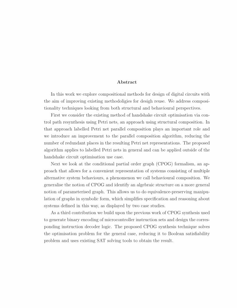
In this work we explore compositional methods for design of digital circuits with
the aim of improving existing methodoligies for desigh reuse. We address composi-
tionality techniques looking from both structural and behavioural perspectives.
First we consider the existing method of handshake circuit optimisation via con-
trol path resynthesis using Petri nets, an approach using structural composition. In
that approach labelled Petri net parallel composition plays an important role and
we introduce an improvement to the parallel composition algorithm, reducing the
number of redundant places in the resulting Petri net representations. The proposed
algorithm applies to labelled Petri nets in general and can be applied outside of the
handshake circuit optimisation use case.
Next we look at the conditional partial order graph (CPOG) formalism, an ap-
proach that allows for a convenient representation of systems consisting of multiple
alternative system behaviours, a phenomenon we call behavioural composition. We
generalise the notion of CPOG and identify an algebraic structure on a more general
notion of parameterised graph. This allows us to do equivalence-preserving manipu-
lation of graphs in symbolic form, which simplifies specification and reasoning about
systems defined in this way, as displayed by two case studies.
As a third contribution we build upon the previous work of CPOG synthesis used
to generate binary encoding of microcontroller instruction sets and design the corres-
ponding instruction decoder logic. The proposed CPOG synthesis technique solves
the optimisation problem for the general case, reducing it to Boolean satisfiability
problem and uses existing SAT solving tools to obtain the result.
Acknowledgements
I am grateful to everyone who made the completion of this work a reality by sharing
their knowledge, assisting directly and supporting me emotionally.
My supervisor, Alex Yakovlev, guided me throughout the research programme
and supported me at all times in many ways. I am thankful to Andrey Mokhov,
Victor Khomenko, Ivan Poliakov and my other colleagues for their contributions to
the work being presented, their participation in discussions and criticism. Special
thanks go to Alexei Iliasov and Danil Sokolov for providing immense help in reviewing
and restructuring the thesis into its present form. Without them this would not have
been possible.
Separate thanks go to the organisations supporting me financially. This work was
supported by a studentship from Newcastle University EECE school, EPSRC grant
EP/G037809/1 (VERDAD) and EPSRC grant EP/K001698/1 (UNCOVER).
ii
Chapter 1
Introduction
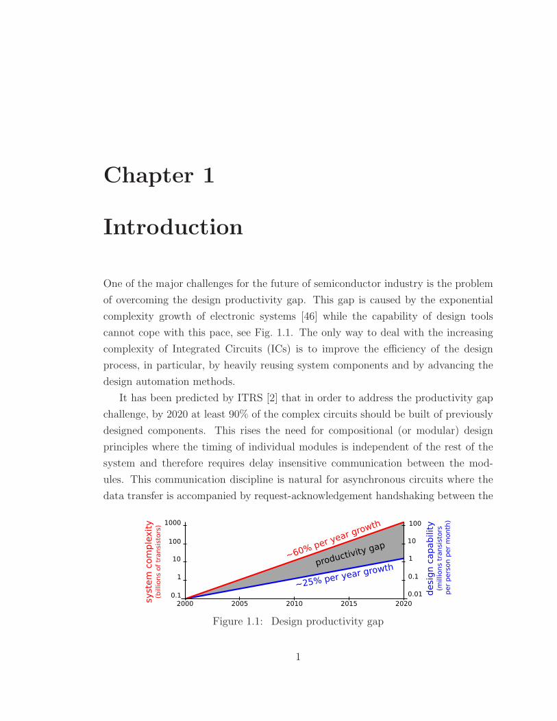
One of the major challenges for the future of semiconductor industry is the problem
of overcoming the design productivity gap. This gap is caused by the exponential
complexity growth of electronic systems [46] while the capability of design tools
cannot cope with this pace, see Fig. 1.1. The only way to deal with the increasing
complexity of Integrated Circuits (ICs) is to improve the efficiency of the design
process, in particular, by heavily reusing system components and by advancing the
design automation methods.
It has been predicted by ITRS [2] that in order to address the productivity gap
challenge, by 2020 at least 90% of the complex circuits should be built of previously
designed components. This rises the need for compositional (or modular) design
principles where the timing of individual modules is independent of the rest of the
system and therefore requires delay insensitive communication between the mod-
ules. This communication discipline is natural for asynchronous circuits where the
data transfer is accompanied by request-acknowledgement handshaking between the
2000 2005 2010 2015 2020
0.1
1
10
100
1000
0.01
0.1
1
10
100
~25% per year growth
~60% per year growth
productivity gap
syste
m c
om
ple
xit
y
(billions o
f tr
ansis
tors
)
desig
n c
apabilit
y(m
illions t
ransis
tors
per
pers
on p
er
month
)
Figure 1.1: Design productivity gap
1
CHAPTER 1. INTRODUCTION
sending and the receiving counterparts. On this pathway the previously designed
Intellectual Property (IP) cores will need to be adapted to the new modular ar-
chitectures. The least intrusive is the Globally Asynchronous Locally Synchronous
(GALS) approach [10] where special wrappers [24,47] are built around synchronous
modules to convert their communication into asynchronous handshake style. Another
alternative is desynchronisation techniques [15] where the global clock is replaced by
a distributed control which determines when the computation is complete and the
output result is ready to be consumed. This control may take different forms, from
a delay line matching the critical path of the module [16] to explicitly introduced
completion detection logic [34].
The remaining 10% of the IC components, as well as the interface and control
logic to support the interconnect and communication flexibility, will still need to
be designed from scratch. One way is to design those components in traditional
synchronous way and then apply the previously discussed techniques to comply with
the delay insensitive interface requirements. This, however, may result in suboptimal
solutions in terms of circuit area, computation speed and energy consumption. Better
results can be achieved if the components are designed and implemented with their
asynchronous environment in mind [36]. However, the logic synthesis of asynchronous
circuits is computationally expensive and not applicable to large modules. This is
due to high level of concurrency in truly asynchronous systems which results in a
state space explosion. The computation complexity problem has been successfully
addressed in the syntax-driven translation [22] approach which is based on direct
mapping of a specification into hardware components without going through the state
space exploration (it is assumed that there is one-to-one correspondence between the
specification language constructs and the library of available components).
The major drawback of the circuits obtained by the syntax-driven translation is
the suboptimal performance of their control structures [53]. In order to resolve this
issue the control models of all the components need to be composed together and
resynthesised exploiting the benefits of their joint optimisation. Existing resynthesis
methods are based on parallel composition of component models expressed in form of
Petri nets [25]. However, the efficient parallel composition of the component models
is still an open question and is one of the primary goals of this thesis.
The composition of circuit components is of structural nature - they are combined
2
CHAPTER 1. INTRODUCTION
operation 1
operation 2
operation 3in out
(a) Structural composition
scenario 1
scenario 2
scenario 3
in out
mode
0
2
0
2
11
(b) Naive behavioural composition
scenario 2
scenario 3
scenario 1
mode
outin
common functionality
(c) Behavioural composition
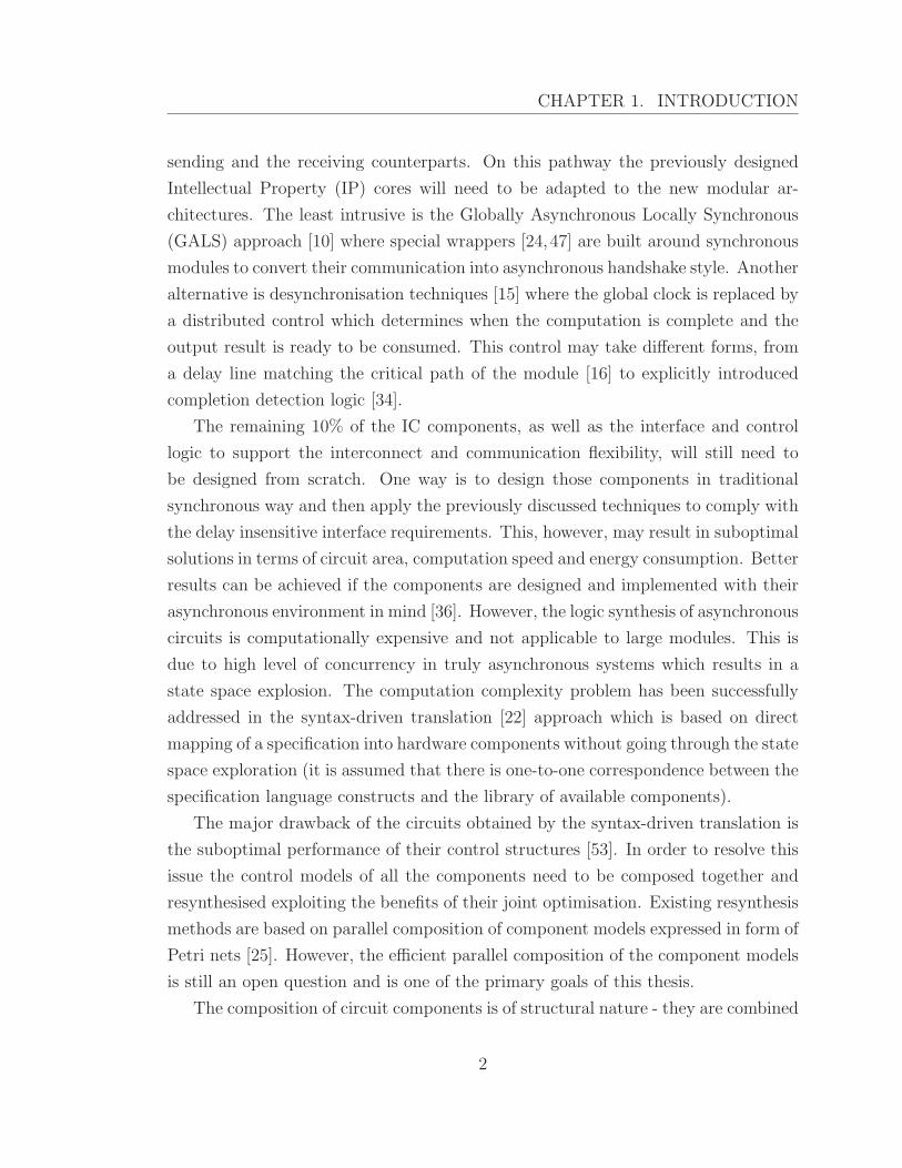
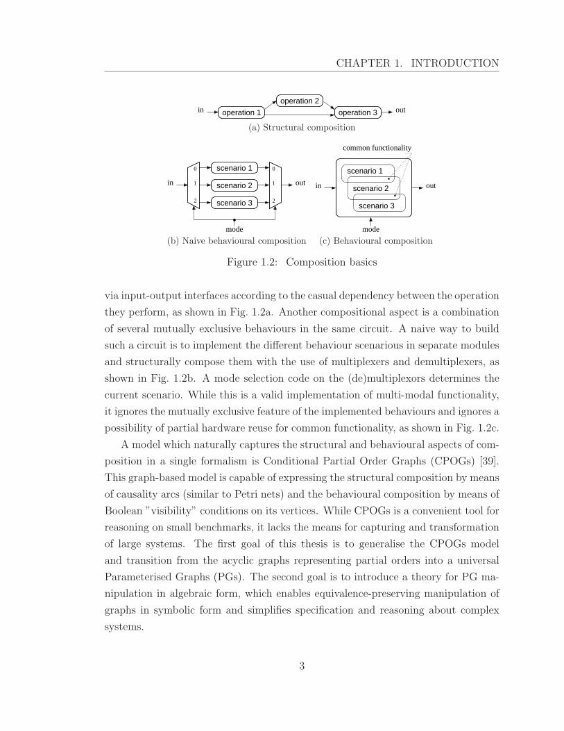
Figure 1.2: Composition basics
via input-output interfaces according to the casual dependency between the operation
they perform, as shown in Fig. 1.2a. Another compositional aspect is a combination
of several mutually exclusive behaviours in the same circuit. A naive way to build
such a circuit is to implement the different behaviour scenarious in separate modules
and structurally compose them with the use of multiplexers and demultiplexers, as
shown in Fig. 1.2b. A mode selection code on the (de)multiplexors determines the
current scenario. While this is a valid implementation of multi-modal functionality,
it ignores the mutually exclusive feature of the implemented behaviours and ignores a
possibility of partial hardware reuse for common functionality, as shown in Fig. 1.2c.
A model which naturally captures the structural and behavioural aspects of com-
position in a single formalism is Conditional Partial Order Graphs (CPOGs) [39].
This graph-based model is capable of expressing the structural composition by means
of causality arcs (similar to Petri nets) and the behavioural composition by means of
Boolean ”visibility” conditions on its vertices. While CPOGs is a convenient tool for
reasoning on small benchmarks, it lacks the means for capturing and transformation
of large systems. The first goal of this thesis is to generalise the CPOGs model
and transition from the acyclic graphs representing partial orders into a universal
Parameterised Graphs (PGs). The second goal is to introduce a theory for PG ma-
nipulation in algebraic form, which enables equivalence-preserving manipulation of
graphs in symbolic form and simplifies specification and reasoning about complex
systems.
3

CHAPTER 1. INTRODUCTION
The Boolean conditions on graph vertices can be expressed in various forms tar-
geting different optimisation criteria. In the context of digital circuit design these
conditions are subsequently implemented as the hardware control logic, therefore
such optimisation targets as minimising the number of control variables and/or re-
ducing the complexity of logical expressions, is of paramount importance. The am-
bitious goal of this thesis is to solve the optimisation problem for the general case,
to express it in terms of Boolean satisfiability problem and to employ the existing
SAT solving tools for obtaining the best result.
1.1 Contributions
The main contributions of the thesis are as follows:
• Improved parallel composition: a novel method for composition of models
specified with labelled Petri Nets.
• PG theory: CPOG generalisation to Parametrised Graph formalism and
mechanised proof of its algebraic properties.
• PG Synthesis: a technique for synthesis of processor instruction decoder
using instruction sets specified with Parametrised Graphs.
• CAD tool support: automation for the above, including improved parallel
composition and encoding of TPG specifications using Workcraft framework.
1.2 Overview
Handshake circuits [7] are widely applied in the design and synthesis of real-life hard-
ware. One prominent problem is obtaining an efficient implementation from a struc-
tural compositional specification. Syntax-based synthesis tools such as Balsa [22] are
unable to take into account the compositional behaviour of STGs corresponding to
handshake circuit components. To address this issue we propose a technique that
selectively composes STGs of related components to obtain a smaller and more per-
formant circuit without suffering state space explosion commonly associated with
4

CHAPTER 1. INTRODUCTION
Petri net based techniques [60]. This transformation, which we refer to as resyn-
thesis [4, 11, 33, 52], is accomplished in three stages. First, we apply a heuristic to
identify the most promising candidates for STG-level composition. Second, we per-
form a parallel composition of the selected component STGs and as a result obtain
a new handshake circuit with custom components, functionally equivalent to a com-
bination of elementary components. Finally, a gate-level implementation is obtained
from the new handshake circuit via a component-wise synthesis of STGs.
Unfortunately, the standard definition of parallel composition almost always
yields a ‘messy’ Petri net, with many implicit places, causing performance deteri-
oration in techniques that are based on structural methods such as the resynthesis
approach. To counter this, we propose an improved algorithm for computing the par-
allel composition. The algorithm generally produces nets with fewer implicit places
that are better suited for subsequent application of structural methods [3].
In addition to purely structural composition of STGs, it is also beneficial to con-
sider a mixture of structural and behavioural composition. Conditional Partial Order
Graphs (CPOG) [39] is a graph-based notation supporting compact representation
and efficient manipulation of both structural and behavioural composition styles.
As one example, when developing complex circuit, it is often necessary to consider
several operational modes of a circuit [44,62]. For this, one needs methodologies and
tools to exploit similarities between the individual modes and hence lift the level of
discourse to behaviour families. This necessitates that behaviours are managed in
a compositional way: the specification of the system must be composed from spe-
cifications of its blocks. Furthermore, since the approach is intended to be a part
of a safety critical toolchain, it is essential that such a specification is amenable to
mechanised reasoning and transformation.
In Chapter 4 we propose an extension of the CPOG formalism, called Paramet-
erised Graph (PG). PGs deal with general graphs rather than just partial orders. We
introduce an algebra of Parameterised Graphs by specifying the equivalence relation
via a set of axioms, which we prove to be sound, minimal and complete [43]. This
result allows one to manipulate a PG model as an algebraic expression applying
the bi-directional rewrite rules of this algebra. This is in contrast to the CPOG
formalism that does not offer a unifying algebraic structure. We demonstrate the
usefulness of the developed formalism with two case studies coming from the area of
5
CHAPTER 1. INTRODUCTION
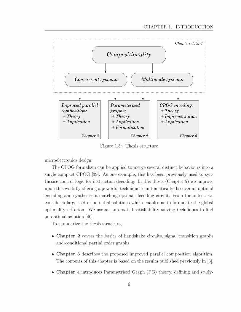
Figure 1.3: Thesis structure
microelectronics design.
The CPOG formalism can be applied to merge several distinct behaviours into a
single compact CPOG [39]. As one example, this has been previously used to syn-
thesise control logic for instruction decoding. In this thesis (Chapter 5) we improve
upon this work by offering a powerful technique to automatically discover an optimal
encoding and synthesise a matching optimal decoding circuit. From the outset, we
consider a larger set of potential solutions which enables us to formulate the global
optimality criterion. We use an automated satisfiability solving techniques to find
an optimal solution [40].
To summarize the thesis structure,
• Chapter 2 covers the basics of handshake circuits, signal transition graphs
and conditional partial order graphs.
• Chapter 3 describes the proposed improved parallel composition algorithm.
The contents of this chapter is based on the results published previously in [3].
• Chapter 4 introduces Parametrised Graph (PG) theory, defining and study-
6
CHAPTER 1. INTRODUCTION
ing an algebraic structure that generalises Conditional Partial Order Graph
formalism. This chapter is based on the results previously published in [43].
• Chapter 5 describes a technique for optimal encoding of processor instruction
sets defined using PG formalism. This chapter is based on the results previously
published in [40]. An earlier version of this paper has qualified for a Best Paper
Award at the ACSD conference.
• Chapter 6 summarises the achieved results and proposes ideas for future
research.
• Appendix contains formal proofs in form of Agda source code for the PG
Algebra properties discussed in Chapter 4.
The relationship between chapters is illustrated in Figure 1.3.
7
Chapter 2
Background
This chapter introduces a brief overview of the major techniques and models used
throughout the thesis. In particular, handshake circuits – a specification formalism
for synthesis of self-timed hardware; Petri nets – a graph-based notation for reasoning
about concurrent behaviour; conditional partial order graphs (CPOG) – a versatile
notation for describing a family of partial orders.
2.1 Handshake circuits
One of the approaches to design of asynchronous circuits is syntax-directed mapping
with handshake circuits as an intermediate format. The parse tree of a program
source code written in a CSP-style [26] language can be interpreted as a graph of
components, connected with communication links called handshake channels. The
components can then be individually mapped to gate-level implementations with
complete circuit derived by implementing the handshake channels with wires.
This approach has been first used by Philips in their Tangram [29] design tool
and later made publicly available when the similar free Balsa [22] system has been
released.
This thesis will be working with Balsa handshake components.
A handshake activation h is said to enclose a process p if p can only start after
h gets a request and h can get an acknowledgement only after p gets finished.
A handshake circuit consists of handshake components which interact by request/
acknowledgment handshaking over communication channels. Each handshake com-
8

CHAPTER 2. BACKGROUND
ponent is specified by a set of ports and a process communicating over those ports.
A protocol is assigned to each port, which specifies whether the process initiates the
handshakes over an active port or awaits for the other party over a passive port. It
also specifies the direction and size of data transferred during the handshakes. Each
channel connects two ports of the same data size with one port being active and
the other being passive. Active input ports and passive output ports are called pull
ports while the pasive input and active output ports are called push ports.
On diagrams used in this thesis we display handshake components with large
circles with a process symbol inside and handshake ports with small circles where
filled circle stands for active port and hollow circle stands for passive port. Channels
are displayed as lines between the corresponding ports with the direction of the arrow
corresponding to the direction of data flow.
The defining feature of a handshake component is the process associated with it.
In Balsa there are about fifty types of processes with each having its own behaviour.
An important notion used to describe behaviours is channel activation. Activ-
ation is a process starting with a request being sent from the active port to the
passive port and ending with an acknowledgement being sent back. The behaviour
of a channel can be described as activation repeated indefinitely. For data channels
activation additionally determines the period of time the values on the data wires
remain valid.
Processes, including activations, are subject to a notion of enclosure to describe
temporal relationship between them. It is said that a process p is enclosed into a
process q when the beginning of p comes after the beginning of q while the end of p
comes before the end end of q.
• Sequence (Fig. 2.1a) is a component with three control ports: a passive port s
and two active ports t1 and t2. The behaviour of the component is as follows:
each activation on s encloses the process consisting of sequential activation on
t1 followed by t2.
• Concur (Fig. 2.1b) is a component with a similar external interface: it has
a passive port s and two active ports t1 and t2. The behaviour is different
though: each activation on s for this component encloses activation of t1 and
t2 concurrently.
9

CHAPTER 2. BACKGROUND
• Sync (Fig. 2.1c) is a component with three control ports: two passive ports s1
and s2 and an active port t. This component ensures enclosure of t into both s1
and s2 by the means of synchronisation between s1 and s2. This component is
dual to Concur in the sense that they form a no-op when their corresponding
ports are connected.
• Call (Fig. 2.1d) is another component with three control ports: two passive
ports s1 and s2 and an active port t. It differs from Sync in that instead of
expecting concurrent activation of both s1 and s2 it only expects one of them
to be activated at a time and encloses t into the one which happens.
• BinaryFunc (Fig. 2.1e) is a component with three pull data ports: a passive
port o and two active ports i1 and i2. It is parametrised on width of those
ports and on a function it computes. Control-wise it is similar to Concur: it
encloses the concurrent activation of i1 and i2 into the activation on o.
• CallMux (Fig. 2.1f) is a component similar to Call with the difference that all
of its ports are further extended to w-bit pull ports. Its behaviour is identical
from the control point of view, with the additional data being received through
t and sent through the activated output port.
• V ariable (Fig. 2.1g) is a component with a single input data port w, called
the write port and a set of passive output data ports r, called read ports. The
component is parameterised on the bit width of the variable w, coinciding with
the width of the data ports. It is also parameterised on the number of read
ports n. The behaviour of V ariable is to remember the data written with the
latest activation of w and to output that data on any activation of a read port
ri. The behaviour is trivial from the control point of view: the only way the
ports interact is through the data. However, there is a requirement that the
write port activation does not overlap with any of the read port activations.
• While (Fig. 2.1h) is a component with a passive control port s, an active
control port t and an active one-bit input data port c. Its behaviour is to
enclose into the activation on s the following process: complete a handshake
over c to obtain the one-bit data indicating the process activity condition; if
this condition holds then activate t and repeat the operations.
10
CHAPTER 2. BACKGROUND
(a) Sequence (b) Concur
.
(c) Sync
|
(d) Call
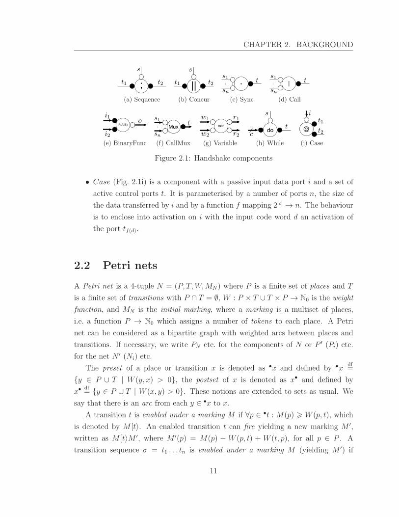
(e) BinaryFunc (f) CallMux (g) Variable (h) While (i) Case
Figure 2.1: Handshake components
• Case (Fig. 2.1i) is a component with a passive input data port i and a set of
active control ports t. It is parameterised by a number of ports n, the size of
the data transferred by i and by a function f mapping 2|c| → n. The behaviour
is to enclose into activation on i with the input code word d an activation of
the port tf(d).
2.2 Petri nets
A Petri net is a 4-tuple N = (P, T,W,MN ) where P is a finite set of places and T
is a finite set of transitions with P ∩ T = ∅, W : P × T ∪ T × P → N0 is the weight
function, and MN is the initial marking, where a marking is a multiset of places,
i.e. a function P → N0 which assigns a number of tokens to each place. A Petri
net can be considered as a bipartite graph with weighted arcs between places and
transitions. If necessary, we write PN etc. for the components of N or P ′ (Pi) etc.
for the net N ′ (Ni) etc.
The preset of a place or transition x is denoted as •x and defined by •xdf=
{y ∈ P ∪ T | W (y, x) > 0}, the postset of x is denoted as x• and defined by
x•df= {y ∈ P ∪ T | W (x, y) > 0}. These notions are extended to sets as usual. We
say that there is an arc from each y ∈ •x to x.
A transition t is enabled under a marking M if ∀p ∈ •t : M(p) > W (p, t), which
is denoted by M [t〉. An enabled transition t can fire yielding a new marking M ′,
written as M [t〉M ′, where M ′(p) = M(p) − W (p, t) + W (t, p), for all p ∈ P . A
transition sequence σ = t1 . . . tn is enabled under a marking M (yielding M ′) if
11

CHAPTER 2. BACKGROUND
M [t1〉M1[t2〉 . . .Mn−1[tn〉Mn = M ′, and we write M [σ〉, M [σ〉M ′ resp.; σ is called
execution of N if MN [σ〉. The empty transition sequence λ is enabled under every
marking. M is called reachable if a transition sequence σ with MN [σ〉M exists.
N is called bounded if, for every reachable markingM and every place p, M(p) 6
k for some constant k ∈ N; if k = 1, N is called safe. N is bounded if and only if
the set [MN〉 of reachable markings is finite. In this thesis, we are mostly concerned
with bounded Petri nets.
A place p is implicit if it can be deleted from the net without changing the set of
executions, and so an implicit place can be removed from the net without affecting
its behaviour.1 Unfortunately, detecting implicit places is expensive: the problem is
PSpace-complete for safe and ExpSpace-complete for general Petri nets. A place p
is duplicate if there is another place p′ with the same pre- and postsets whose initial
marking does not exceed that of p. Duplicate places are implicit, and are cheap to
detect.
An STG is a tuple N = (P, T,W,MN , In,Out, ℓ) where (P, T,W,MN ) is a Petri
net and In and Out are disjoint sets of input and output signals. For Sig = In∪Out
being the set of all signals, ℓ : T → Sig × {+,−} ∪ {λ} is the labelling function.
Sig × {+,−} or short Sig± is the set of signal transitions ; its elements are denoted
as s+, s− resp. instead of (s,+), (s,−) resp. A plus sign denotes that a signal value
changes from logical low (written as 0) to logical high (written as 1), and a minus
sign denotes the opposite direction. We write s± if it is not important or unknown
which direction takes place.
An STG can contain transitions labelled with λ, called dummy transitions, which
do not correspond to any signal change. Hiding a signal s means to change the label
of all transitions labelled with s± to λ. (The idea of re-synthesis approach is to hide
the signals used for communication between components, which results in an STG
with fewer signals that often has a simpler implementation as a circuit.) The labelling
of an STG is called injective if for each pair of distinct non-dummy transitions t and
t′, ℓ(t) 6= ℓ(t′).
Examples of STGs are shown in Figs. 3.1 and 3.2. Places are drawn as circles
containing a number of tokens corresponding to the initial marking. Unmarked
places which have only one transition in their presets and postsets are not drawn if
1Note that an implicit place can cease to be implicit if another implicit place is removed first.
12
CHAPTER 2. BACKGROUND
the corresponding arcs have the weight 1; they are implicitly given by an arc between
these two transitions (and if such a place contains tokens, they are drawn on the arc
itself). Transitions are drawn simply as their labels, and the weight function is
drawn as directed arcs (x, y) whenever W (x, y) 6= 0 (and labelled with W (x, y) if
W (x, y) > 1).
We lift the notion of enabledness to transition labels: we write M [ℓ(t)〉〉M ′ if
M [t〉M ′. This is extended to sequences as usual – deleting λ-labels automatically
since λ is the empty word; i.e. M [s±〉〉M ′ means that a sequence of transitions fires,
where one of them is labelled s± while the others (if any) are λ-labelled. A sequence
ν ∈ (Sig±)∗ is called a trace of a marking M if M [ν〉〉, and a trace of N if M =MN .
The language L(N) of N is the set of all traces of N .
The reachability graph RG(N) of an STG N is an arc-labelled directed graph on
the reachable markings of N with MN as the root; there is an arc from M to M ′
labelled ℓ(t) whenever M [t〉M ′. For bounded Petri nets and STGs, RG(N) can be
seen as a finite automaton (where all states are accepting), and L(N) is the language
of this automaton. Observe that automata with accepting states only can be regarded
as STGs (with the states as places, the initial state being the only marked place,
etc.); hence, all definitions for STGs also apply to automata.
N is deterministic if RG(N) is a deterministic automaton: it contains no λ-
labelled transitions and there are no dynamic auto-conflicts, i.e. for each reachable
marking M and each signal transition s± there is at most one M ′ with M [s±〉〉M ′.
(Note that a deterministic STG can have choices between different outputs, e.g. an
STG modelling the standard arbiter is deterministic).
An STG with a set of all markings S2 is said to simulate another STG with a set
of all markings S1 iff there exist an R ⊆ S1 × S2 such that (MN1,MN2) ∈ R and for
any pair of markings (M1,M2) ∈ R, a label l and a marking M ′1, M1[l〉〉M
′1 implies
M2[l〉〉M′2 for some M ′
2. We call R the witness of simulation. Now we can say that
STGs N1 and N2 are bisimilar iff N2 simulates N1 with witness R and N2 simulates
N1 with witness R−1.
For deterministic STGs, language equivalence and bisimulation coincide, and the
language can be taken as the semantics of such a specification. Unfortunately, the
class of deterministic STGs is too restrictive in practice [31], e.g.:
13
CHAPTER 2. BACKGROUND
• using dummy transitions is often convenient in manual design;
• modelling OR-causality [63] as a safe STG requires non-determinism;
• hiding internal communication (and thus introducing dummy transitions) is a
crucial step in re-synthesis.
Hence, one has to deal with non-deterministic STGs as well.
One might think that if RG(N) is non-deterministic, it can be determinised (us-
ing well-known automata-theoretic methods), i.e. turned into a language-equivalent
deterministic automaton with accepting states only; in particular, the resulting auto-
maton will have no λ-arcs. Unfortunately, this is a bad idea, as shown in [31], where
the semantics of non-deterministic STGs was developed. It is based on the concept
of output-determinacy, which is a relaxation of determinism: An STG N is output-
determinate (OD) if MN [ν〉〉M1 and MN [ν〉〉M2 implies for every x ∈ OutN that
M1[x±〉〉 iff M2[x
±〉〉. It turns out that OD STGs are exactly the STGs which have
correct implementations according to the implementation relation introduced in [31].
Hence, non-OD STGs are ill-formed, and in particular cannot be correctly imple-
mented as circuits. This shows that in general, the language is not a satisfactory
semantics of non-deterministic STGs; in particular, synthesising the determinised
reachability graph of a non-OD STG will either fail or result in an incorrect circuit.
On the other hand, for the class of OD STGs [31] shows that their language is an
adequate semantics, and implementation relation can be formulated purely in terms
of the language. An important property of OD STGs is that in them the enabledness
of an output signal is a function of the trace, i.e. given a trace ν, the set of outputs
by which ν can be extended is uniquely determined, even though there could be
multiple executions corresponding to ν.
In the following definition of parallel composition ‖, see e.g. [61], we will have
to consider the distinction between input and output signals. The idea of parallel
composition is that the composed systems run in parallel and synchronise on common
actions – corresponding to circuits that are connected on the wires corresponding
to the signals. Since a system controls its outputs, we cannot allow a signal to be
an output of more than one component; input signals, on the other hand, can be
shared. An output signal of a component may be an input of other components, and
in any case it is an output of the composition.
14
CHAPTER 2. BACKGROUND
The parallel composition of STGs N1 and N2 is defined if Out1∩Out2 = ∅. If we
drop this requirement, the definition gives the synchronous product N1×N2, which is
often useful. The place set of the composition is the disjoint union of the place sets of
the components; therefore, we can consider markings of the composition (regarded as
multisets) as the disjoint union of markings of the components, and we will also write
such a marking M1∪M2 of the composition as (M1,M2). To define the transitions,
let A = (In1∪Out1)∩(In2∪Out2) be the set of common signals. If e.g. s is an output
of N1 and an input of N2, then firing of s± in N1 is ‘seen’ by N2, i.e. it must be
accompanied by firing of s± in N2. Since we do not know a priori which s±-labelled
transition of N2 will fire together with some s±-labelled transition of N1, we have
to allow for each possible pairing. Thus, the parallel composition N = N1 ‖ N2 is
obtained from the disjoint union of N1 and N2 by fusing each s±-labelled transition
t1 of N1 with each s±-labelled transition t2 from N2 if s ∈ A. Such transitions
are pairs and the firing (M1,M2)[(t1, t2)〉(M′1,M
′2) of N corresponds to the firings
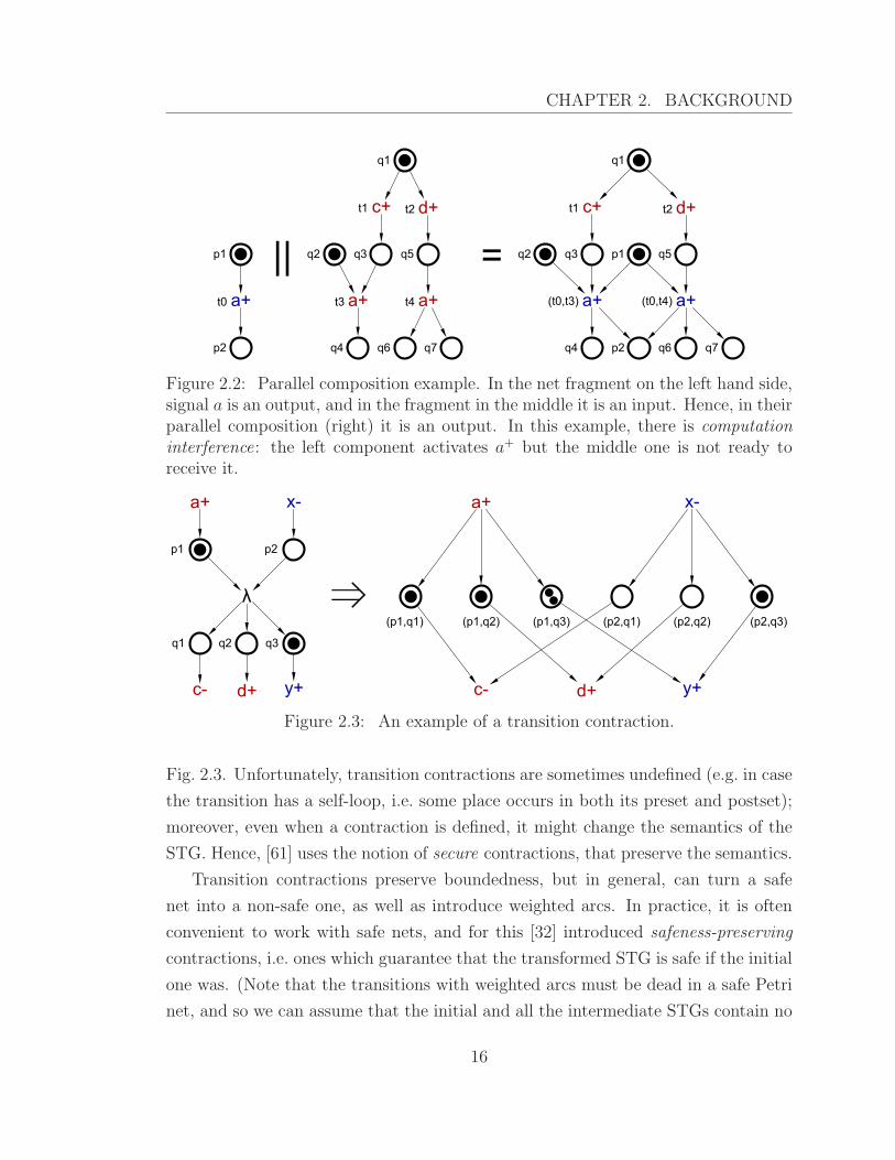
Mi[ti〉M′i in Ni, i = 1, 2; for an example of a parallel composition, see Fig. 2.2. More
generally, we have (M1,M2)[ν〉〉(M′1,M
′2) iff Mi[ν|Ni
〉〉M ′i for i ∈ {1, 2}, where ν|Ni
denotes the projection of the trace ν onto the signals of the STG Ni. Hence, all
reachable markings of N have the form (M1,M2), where Mi is a reachable marking
of Ni, i = 1, 2.
Obviously, one can extend the notion of the parallel composition to a finite family
(or collection) (Ci)i∈I of STGs as ‖i∈I Ci, provided that no signal is an output
signal of more than one of the Ci. We will also denote the markings of such a
composition by (M1, . . . ,Mn) if Mi is a marking of Ci for i ∈ I = {1, ..., n}. As
above, (M1,M2, . . . ,Mn)[ν〉〉(M′1,M
′2, . . . ,M
′n) iff Mi[ν|Ci
〉〉M ′i for all i ∈ {1, . . . , n}.
It is easy to see that C is deterministic if all Ci are. However, this is not true for a
composition of OD STGs, as the result, in general, can be non-OD in such a case.
A composition can also be ill-defined due to computation interference, see e.g. [20].
Let Cdf=‖i∈I Ci be a composition of STGs. It is free from computation interference
(FCI) if for every trace ν of C the following holds: if ν|Cjx± is a trace of Cj for some
output x of Cj, then ν|Cx± is a trace of C.
Transition contraction [61] is an important operation in circuit re-synthesis. It
removes a dummy transition from an STG and combines each place of its preset
with each place of its postset to ‘simulate’ the firing of the deleted transition, see
15
CHAPTER 2. BACKGROUND
p1
p2
t0
q2 q3
t3
q4
t1 t2
q1
q5
q6 q7
t4
q1
t1 t2
q3q2 p1 q5
(t0,t3) (t0,t4)
q4 p2 q6 q7
|| =
Figure 2.2: Parallel composition example. In the net fragment on the left hand side,signal a is an output, and in the fragment in the middle it is an input. Hence, in theirparallel composition (right) it is an output. In this example, there is computationinterference: the left component activates a+ but the middle one is not ready toreceive it.
p1 p2
q1 q2 q3
(p1,q1) (p1,q2) (p1,q3) (p2,q1) (p2,q2) (p2,q3)
λ ⇒
Figure 2.3: An example of a transition contraction.
Fig. 2.3. Unfortunately, transition contractions are sometimes undefined (e.g. in case
the transition has a self-loop, i.e. some place occurs in both its preset and postset);
moreover, even when a contraction is defined, it might change the semantics of the
STG. Hence, [61] uses the notion of secure contractions, that preserve the semantics.
Transition contractions preserve boundedness, but in general, can turn a safe
net into a non-safe one, as well as introduce weighted arcs. In practice, it is often
convenient to work with safe nets, and for this [32] introduced safeness-preserving
contractions, i.e. ones which guarantee that the transformed STG is safe if the initial
one was. (Note that the transitions with weighted arcs must be dead in a safe Petri
net, and so we can assume that the initial and all the intermediate STGs contain no
16

CHAPTER 2. BACKGROUND
such arcs.) Also, [32] developed a sufficient structural condition for a contraction to
be safeness-preserving.
From the point of view of this thesis, it is important to remark that implicit places
can adversely affect the (secure) contractibility of a transition, i.e. it is possible to
have a situation when a transition is not contractible (or not securely contractible),
but becomes securely contractible after some implicit place is removed from the STG.
As detecting implicit places is expensive, it is very desirable to reduce their number
by some other means, in particular the approach proposed in this thesis reduces the
number of such places in STGs obtained by parallel composition. This has a direct
effect on re-synthesis: if the composed STG has fewer implicit places, more dummy
transitions in it can be contracted, and so it will be easier to synthesise the result.
2.3 Conditional Partial Order Graphs
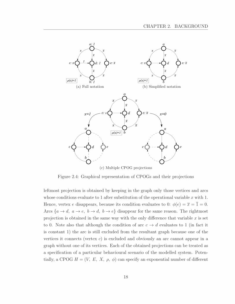
A Conditional Partial Order Graph (CPOG) [39][45] is a quintupleH = (V, E, X, ρ, φ),
where V is a finite set of vertices, E ⊆ V ×V is a set of arcs between them, and X is
a finite set of operationalvariables. An opcode is an assignment (x1, x2, . . . , x|X|) ∈
{0, 1}|X| of these variables; X can be assigned only those opcodes which satisfy the
restriction function ρ of the graph, i.e. ρ(x1, x2, . . . , x|X|) = 1. Function φ assigns
a Boolean condition φ(z) to every vertex and arc z ∈ V ∪ E of the graph.
Figure 2.4(a) shows an example of a CPOG containing |V | = 5 vertices and
|E| = 7 arcs. There is a single operational variable x; the restriction function is
ρ(x) = 1, hence both opcodes x = 0 and x = 1 are allowed. Vertices {a, b, d} have
constant φ = 1 conditions and are called unconditional, while vertices {c, e} are
conditional and have conditions φ(c) = x and φ(e) = x respectively. Arcs also fall
into two classes: unconditional (arc c→ d) and conditional (all the rest). As CPOGs
tend to have many unconditional vertices and arcs we use a simplified notation in
which conditions equal to 1 are not depicted in the graph. This is demonstrated in
Figure 2.4(b).
The purpose of conditions φ is to ‘switch off’ some vertices and/or arcs in the
graph according to the given opcode. This makes CPOGs capable of specifying
multiple partial orders or instructions (a partial order is a form of behavioural de-
scription of an instruction). Figure 2.4(c) shows a graph and its two projections. The
17
CHAPTER 2. BACKGROUND
a: 1
d: 1
b: 1
c: x e: x_
x
x
1
x _
x _
x _
x _
ρ(x)=1
(a) Full notation
a
d
b
c: x e: x_
x
x
x _
x _
x _
x _
ρ(x)=1
(b) Simplified notation
a
d
b
c: x e: x_
x
x
x _
x _
ρ(x)=1
a
d
b
c e
x=1
a
d
b
c e
x=0
x _
x _
(c) Multiple CPOG projections
Figure 2.4: Graphical representation of CPOGs and their projections
leftmost projection is obtained by keeping in the graph only those vertices and arcs
whose conditions evaluate to 1 after substitution of the operational variable x with 1.
Hence, vertex e disappears, because its condition evaluates to 0: φ(e) = x = 1 = 0.
Arcs {a → d, a → e, b → d, b → e} disappear for the same reason. The rightmost
projection is obtained in the same way with the only difference that variable x is set
to 0. Note also that although the condition of arc c → d evaluates to 1 (in fact it
is constant 1) the arc is still excluded from the resultant graph because one of the
vertices it connects (vertex c) is excluded and obviously an arc cannot appear in a
graph without one of its vertices. Each of the obtained projections can be treated as
a specification of a particular behavioural scenario of the modelled system. Poten-
tially, a CPOG H = (V, E, X, ρ, φ) can specify an exponential number of different
18
CHAPTER 2. BACKGROUND
partial orders of events in V according to one of 2|X| different possible opcodes.
A CPOG is well-defined if all its projections allowed by ρ are acyclic. We consider
only well-defined CPOGs in this thesis, because a cyclic projection has no natural
execution semantics, in particular it is not clear which event can be executed first
unless some form of a ‘token’ is introduced as in the Petri Net model [14].
To summarise, a CPOG is a structure to represent a set of encoded partial orders
in a compact form. Synthesis and optimisation methods presented in [45] provide a
way to obtain such a representation given a set of partial orders and their opcodes.
For example, the CPOG in Figure 2.4(c) can be synthesised automatically from the
two partial orders below it and the corresponding opcodes x = 1 and x = 0. The
next section shows that a particular assignment of opcodes to the partial orders has
a strong impact on the final CPOG, therefore in order to obtain the most compact
CPOG representation one has to search for the best opcode assignment.
Note that partial orders is not the only formalism for formal specification of in-
structions. In particular, there is an alternative approach [6] based on automata,
which treats every instruction as a burst-mode state machine and defines an opera-
tion of composition on them. While benefiting from a direct correspondence between
flowcharts of algorithms and automata, the approach cannot model true concurrency:
a set of causally independent events can only be executed as a ‘burst’ in the same
step/clock cycle. Also, it requires explicit memory to track the current state of the
automaton. We believe that partial orders are better suited for modelling instruc-
tion sets of processing units built on heterogeneous platforms, i.e. exhibiting both
asynchronous and synchronous interactions [41].
2.4 Agda
Agda [49] is a system serving both as a programming language and as a proof as-
sistant simultaneously. When viewed as a programming language, it is a purely
functional language with its syntax largely inspired by Haskell. Its main distinguish-
ing features are totality (the fact that every function is defined on every possible
input) and dependent typing system that allows for types to depend on the values.
19
CHAPTER 2. BACKGROUND
2.4.1 Function definitions and algebraic data types
A very common language construct in Agda is a function definition. Function defin-
ition must consist of type signature followed by its defining equations. As a simple
example, consider this Boolean exclusive OR function:
xor : Bool → Bool → Bool
xor x y = x ∧ (¬ y) ∨ y ∧ (¬ x )
Here we define a function called xor of type Bool → Bool → Bool with two
arguments x and y defined in terms of ∧ , ∨ and ¬ .
Functions can have more than one defining equation when each equation defines
the function for a particular shape, or pattern of arguments. This is called pattern
matching. For example, the Boolean negation function can be defined the following
way:
¬ : Bool → Bool
¬ false = true
¬ true = false
A more interesting example would be a Boolean AND:
∧ : Bool → Bool → Bool
true ∧ true = true
∧ = false
This example demonstrates an additional feature of pattern matching: equations
are ordered and the earlier ones take precedence.
In the above we used the Bool data type to represent Boolean values. This data
type is not a built-in language construct of Agda, but can be defined using the data
keyword:
data Bool : Set where
true : Bool
false : Bool
Here definition gives the name for the type and lists constructors of its values:
true and false. In this case constructors have no arguments, thus corresponding
20
CHAPTER 2. BACKGROUND
to individual values, but in general a single constructor can correspond to multiple
values, as will be shown later.
2.4.2 Inductive types and recursion
We often want to reason about data types with infinite number of values, such as
natural numbers. To represent them we use inductive type definitions:
data N : Set where
zero : N
suc : N → N
Here we define natural numbers as something that has two forms: it is either a
zero, or a successor suc x where x is another natural number. These two constructors
allow us to construct an arbitrary number of values of type N by successive applica-
tion of suc to zero: zero corresponds to 0, suc zero corresponds to 1, suc (suc zero)
to 2, etc.
To manipulate the values of inductive data types we use recursive functions:
+ : N → N → N
zero + y = y
suc x + y = suc (x + y)
Here we define natural number addition recursively by considering the cases for
the first argument: the base case of 0 + y must evaluate to y and for the recursive
case (1 + x) + y must evaluate to 1 + (x + y). The Agda compiler checks that the
arguments to the function become smaller on recursive calls, thus ensuring that only
well-behaved (terminating) definitions are admitted.
2.4.3 Indexed types and propositions
There is a close correspondence between types and logic, a phenomenon known as
Curry-Howard correspondence. Specifically, types can be thought of as propositions
where the type is inhabited if and only if the corresponding proposition holds true.
Similarly, well-typed terms can be thought of as proofs of the corresponding propos-
itions. Consequently, the type-checker can be used as a proof checker.
21
CHAPTER 2. BACKGROUND
With the language features described so far we can construct types ⊤ and ⊥
corresponding to true (logical tautology) and false (logical contradiction). These are
not to be confused with true and false values of type Bool that can not be used as
types.
data ⊤ : Set where
tt : ⊤
data ⊥ : Set where
Here the type ⊤ has a constructor tt , which makes it inhabited, thus corres-
ponding to the logic value of true. The type ⊥ has no constructors, which makes it
uninhabited, thus corresponding to false.
To construct more complex propositions Agda provides parameterised types, de-
pendent function types and indexed inductive data families.
Type parameters are a basic way to allow for generic data types or logic operators.
Consider the following example:
data Both (A : Set) (B : Set) : Set where
both : A → B → Both A B
data Either (A : Set) (B : Set) : Set where
left : A → Either A B
right : B → Either A B
Here, Both A B can be thought of as a type of tuples of the form both x y with
x : A and y : B . At the same time, for propositions P and Q , Both P Q can be
thought of as their conjunction so that the proof both p q can be constructed if and
only if both p and q (proofs of P and Q) can be constructed.
Similarly, Either is playing a dual role of taking the disjoint union of its type
parameters and the logical disjunction operator. Type Either P Q is inhabited if
and only if types P or Q or both are inhabited.
Another way to define parameterised types is to compute them as a result of a
function.
Consider some examples:
Not : Set → Set
Not P = P → ⊥
22
CHAPTER 2. BACKGROUND
IsTrue : Bool → Set
IsTrue true = ⊤
IsTrue false = ⊥
Not takes a type P and computes another type Not P , which is inhabited if and
only if contradiction is derivable from P . It is useful to think of Not P as being
inhabited if and only if P is not.
IsTrue x is a type that is inhabited if and only if a Boolean value x happens to
equal true.
Dependent function types have the form (x : X ) → Y where x can be free in
Y . This lets the type of the function result to depend on the value passed in as the
argument. In the case when Y is a logical proposition, the dependent type can be
thought of as universal quantification over x . Indeed, let us construct a value that
can serve as a proof that for any boolean value x one of x and ¬ x must be true:
lemma1 : (x : Bool) → Either (IsTrue x ) (IsTrue (¬ x ))
lemma1 true = left tt
lemma1 false = right tt
Finally, indexed inductive type families give you more flexibility by having the
constructor choose the values for type parameter instead of having to construct a
type for a given parameter value:
data IsEven : N → Set where
zero : IsEven 0
suc : (n : N) → IsEven n → IsEven (suc (suc n))
Here IsEven n is inhabited if and only if n is an even number.
With dependent functions it is often useful to omit some of the arguments because
their values are uniquely determined by the types of the arguments that follow. To
be able to do that you can mark the corresponding parameter as implicit by putting
it in curly braces:
lemma2 : {x : N} → IsEven x → Not (IsEven (suc x ))
lemma2 zero ()
lemma2 (suc e) (suc z ) = lemma2 e z
23
CHAPTER 2. BACKGROUND
3 −not − even : Not (IsEven (suc (suc (suc zero))))
3 −not − even = lemma2 (suc zero)
Here the special syntax of () is used to indicate that we are doing a pattern
matching on a given parameter with no cases to choose from. This situation allows
you to complete the definition without having to give a right-hand side.
Of special importance is the equality type, ≡ : {A : Set } → (x : A) → (y :
A) → Set . We have x ≡ y inhabited if and only if x and y are the same value. It is
useful for equational reasoning that is often more natural than inductive proofs.
24
Chapter 3
Improved Parallel Composition
The contents of this chapter is based on the results published previously in [3]. The
chapter covers in detail the proposed modification to the labelled Petri nets parallel
composition algorithm allowing for simpler resulting nets while preserving result
equivalence up to bisimulation.
3.1 Introduction
Parallel composition (synchronous product) of labelled Petri nets is a fundamental
operation in modular hardware design. It is often used to combine models of subsys-
tems into a model of the whole system. In particular, there is a direct correspondence
between parallel composition of Signal Transition Graphs (STGs), a class of labelled
Petri nets used for modelling asynchronous circuits, and connecting circuits by wires.
Hence performing this operation efficiently is important in practice.
Unfortunately, the standard definition of parallel composition almost always
yields a ‘messy’ Petri net, with many implicit places even when the component
Petri nets did not have them. Some of these places are computationally cheap to
remove (e.g. duplicate places – places with identical pre- and postsets). In general,
however, for removing remaining implicit places one needs full-blown model check-
ing, something infeasible if the resulting composition is large [57]. Although implicit
places do not have noticeable effect on tools based on state space exploration, such
as Petrify [13], the performance of tools that are based on structural methods,
such as DesiJ [56], often deteriorates.
25
CHAPTER 3. IMPROVED PARALLEL COMPOSITION
(a) Toggle
(b) Call
(c) Environment (d) Composition
Figure 3.1: Example of standard STG composition.
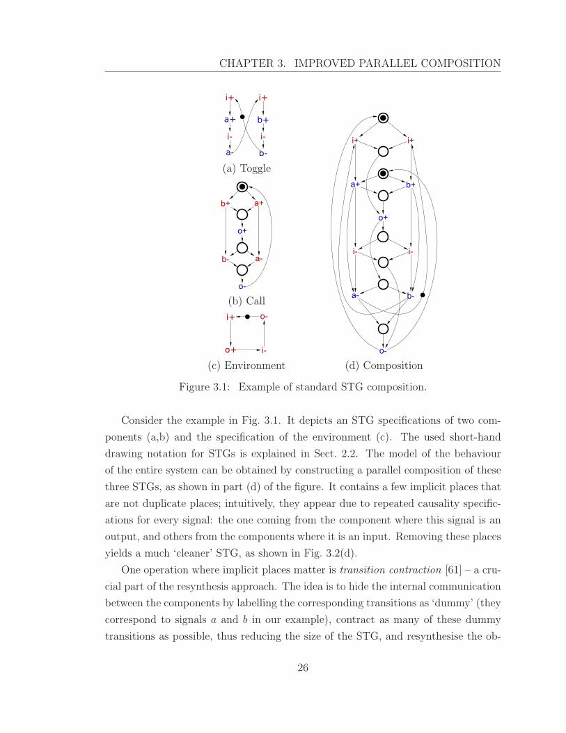
Consider the example in Fig. 3.1. It depicts an STG specifications of two com-
ponents (a,b) and the specification of the environment (c). The used short-hand
drawing notation for STGs is explained in Sect. 2.2. The model of the behaviour
of the entire system can be obtained by constructing a parallel composition of these
three STGs, as shown in part (d) of the figure. It contains a few implicit places that
are not duplicate places; intuitively, they appear due to repeated causality specific-
ations for every signal: the one coming from the component where this signal is an
output, and others from the components where it is an input. Removing these places
yields a much ‘cleaner’ STG, as shown in Fig. 3.2(d).
One operation where implicit places matter is transition contraction [61] – a cru-
cial part of the resynthesis approach. The idea is to hide the internal communication
between the components by labelling the corresponding transitions as ‘dummy’ (they
correspond to signals a and b in our example), contract as many of these dummy
transitions as possible, thus reducing the size of the STG, and resynthesise the ob-
26

CHAPTER 3. IMPROVED PARALLEL COMPOSITION
(a) Toggle
(b) Call
(c) Environment (d) Composition
Figure 3.2: Example of improved STG composition: the components are obtainedfrom the corresponding ones in Fig. 3.1 by removing some places, and then thestandard parallel composition is applied to these modified components.
tained STG as a circuit. The result is often smaller than the original circuit due to
removal of some signals. Transition contraction is normally performed on very large
STGs, such as those corresponding to the whole control path of the circuit, and so,
for efficiency, it has to be a structural operation. However, such structural contrac-
tions are not always possible (see Sect. 2.2), and implicit places in the pre-set and/or
post-set of a transition can prevent contracting it, even if a contraction is possible
after removing these implicit places. In the example in Fig. 3.1(d), DesiJ [56] can-
not contract any of the dummy transitions, even though it performs some structural
tests for place redundancy. Yet, it is able to contract all the dummy transitions if
the implicit places are removed, i.e. when applied to the STG in Fig. 3.2(d).
In Chapter 3 we present a new method for computing the parallel composition
of labelled Petri nets that generates fewer implicit places. It uses the freeness from
computation interference (FCI) assumption [20] stating that it is impossible that
27
CHAPTER 3. IMPROVED PARALLEL COMPOSITION
when one component wants to produce an output it is prevented from doing so
by another component not ready to receive it. Violation of the FCI assumption
means that the behaviour of the composition does not correspond to that of an
implied physical system. For example, an output of a circuit component cannot be
physically disabled by another component that is not ready to receive this signal,
and so producing this output will lead to a malfunction. However, the composition
will be oblivious to the presence of the malfunction and behave as if such an output
could not be produced. Hence FCI is a basic correctness requirement – whenever
it is violated there is no point in computing a parallel composition since it would
not characterise an intended behaviour. In practice, FCI is often guaranteed by
construction, e.g. its satisaction is guaranteed for the control path of a Balsa [21]
or Haste/Tangram [8, 51] specification of an asynchronous circuit. The idea of
using the FCI condition is reminiscent of the method of input/output exposure in
the synthesis by direct mapping described in [59] and of the correct by construction
composition of Petri nets for circuit components and the environment used in the
DI2PN tool [28].
The essence of the proposed method is illustrated by the example in Fig. 3.2.
Before computing a parallel composition, one can remove some of the places in the
components (see (a–c) in Fig. 3.2) and then compose the modified STGs. The precise
conditions that allow us to remove a particular place will be stated in Sect. 3.2. At
this point we shall only mention that they are structural and thus can be efficiently
checked. The method guarantees that the number of places in the resulting Petri net
is not larger and often much smaller (as the number of places in the composition is
the total number of places in all the components), and, under the FCI assumption,
the resulting behaviour is the same up to bisimularity. In the example, composing the
modified components yields the STG in Fig. 3.2(d), containing no implicit places.
The modified components may include unconstrained transitions and unbounded
places and thus be non-implementable. Fortunately, this does not matter, as they
are never used on their own, but only in composition with other components, and
the resulting behaviour of the composition is guaranteed to correspond to that of
the standard composition.
Resynthesis (Section 3.6) of asynchronous circuits is the intended application
of the proposed method. However, we envisage that it may find a much wider
28

CHAPTER 3. IMPROVED PARALLEL COMPOSITION
applicability since composition of labelled Petri nets is a fundamental operation and
the FCI assumption is often known to hold for practically important examples.
3.2 Improved parallel composition
The improved parallel composition algorithm extends the conventional one by adding
a pre-processing step, where some places are removed from the components, as they
are guaranteed to be implicit in the result. To identify these places, one can note
that a place is required in the final composition only if under some reachable marking
it can be the place that disables some transition in its postset.
For simplicity, consider the parallel composition C = C1 ‖ C2, whose components
synchronise on a single signal s which is an output of C1 and an input of C2. Let
(M1,M2) be a reachable marking of C, where M1 and M2 are some reachable mark-
ings of C1 and C2, respectively. Furthermore, suppose that M1 enables, say, s+ in
C1, where s is an output. Now, if M2 does not enable s+ in C2, where s is an input,
then there is computation interference. Therefore, if the FCI assumption holds, M2
has to enable s+ in C2, i.e. whenever s+ is enabled in C1, it is also enabled in C2. In
other words, the firing of s+ in C is fully controlled by C1, and so the constraints on
firing of s that are present in C2 can be ignored. This means that the places in the
preset of an s+-labelled transition in C2 will be implicit in the composition (subject
to some technical conditions formulated below), and so can be removed before the
composition is performed.
The above is true for the simple case of STGs with injective labelling and no
dummies. However, the general picture is more complicated. In case of non-injective
labelling, there can be multiple transitions corresponding to the same input signal
transition, and the FCI assumption only guarantees the enabledness of one of them.
Hence, some ‘memory’ (in the form of places) is required to trace which of these
transitions has to be fired, which prohibits the removal of places from their presets.
Furthermore, if the STG contains dummies, removing places from their postsets
introduces some undesirable effects explained later. These considerations lead to the
following conditions of applicability of the proposed optimisation.
Proposition 1. 1 Let Cdf=‖i∈I Ci be a composition of STGs that satisfies the FCI
1Note that in our previous work [3] we claimed a stronger equivalence (viz. isomorphism of
29
CHAPTER 3. IMPROVED PARALLEL COMPOSITION
1S 2S
1S’ 2S’
1S
1S’
2S
2S’
||
|| plac
e re
mov
al
bisimulation
plac
e re
mov
al
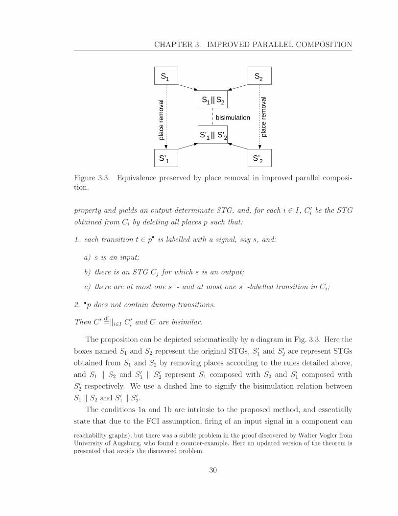
Figure 3.3: Equivalence preserved by place removal in improved parallel composi-tion.
property and yields an output-determinate STG, and, for each i ∈ I, C ′i be the STG
obtained from Ci by deleting all places p such that:
1. each transition t ∈ p• is labelled with a signal, say s, and:
a) s is an input;
b) there is an STG Cj for which s is an output;
c) there are at most one s+- and at most one s−-labelled transition in Ci;
2. •p does not contain dummy transitions.
Then C ′ df=‖i∈I C
′i and C are bisimilar.
The proposition can be depicted schematically by a diagram in Fig. 3.3. Here the
boxes named S1 and S2 represent the original STGs, S ′1 and S ′
2 are represent STGs
obtained from S1 and S2 by removing places according to the rules detailed above,
and S1 ‖ S2 and S ′1 ‖ S ′
2 represent S1 composed with S2 and S ′1 composed with
S ′2 respectively. We use a dashed line to signify the bisimulation relation between
S1 ‖ S2 and S ′1 ‖ S
′2.
The conditions 1a and 1b are intrinsic to the proposed method, and essentially
state that due to the FCI assumption, firing of an input signal in a component can
reachability graphs), but there was a subtle problem in the proof discovered by Walter Vogler fromUniversity of Augsburg, who found a counter-example. Here an updated version of the theorem ispresented that avoids the discovered problem.
30
CHAPTER 3. IMPROVED PARALLEL COMPOSITION
λ λ
⇒
λ λ
Figure 3.4: Example of an STG where removal of places in the postset of dummytransitions results in a wrong behaviour.
be controlled from the outside (viz. by the component controlling the corresponding
output — whose existence is ensured by 1b), and so the component itself can get rid
of the places controlling it.
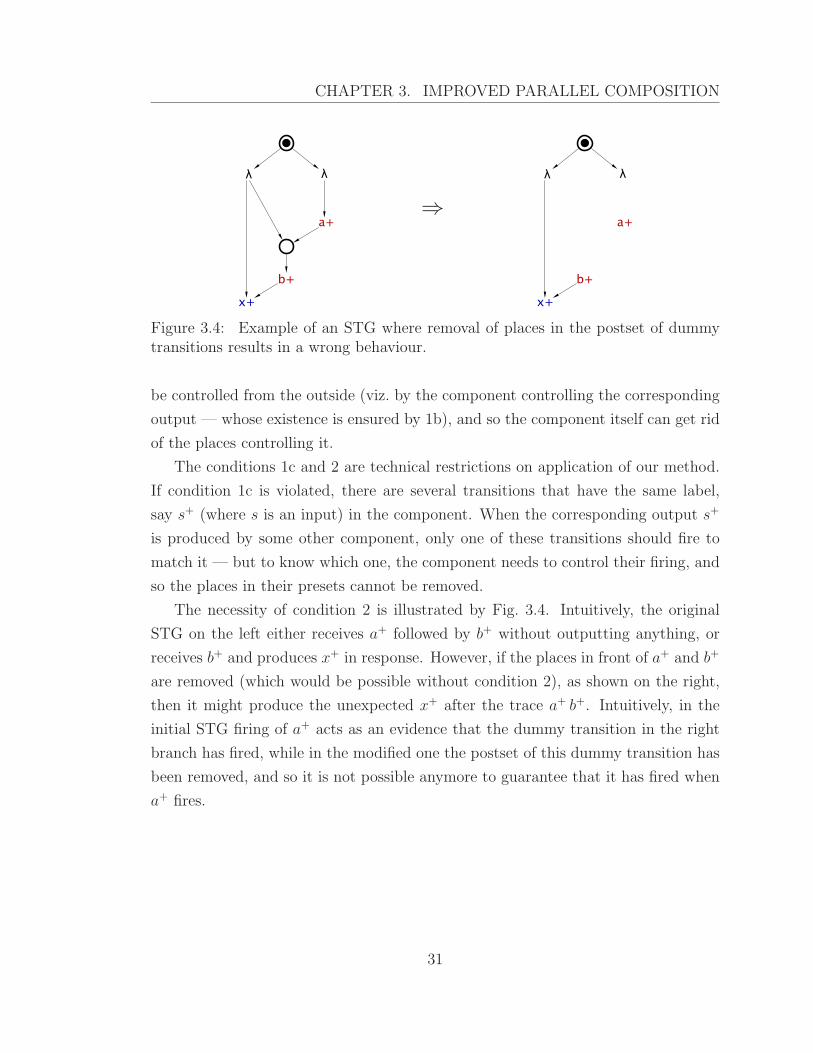
The conditions 1c and 2 are technical restrictions on application of our method.
If condition 1c is violated, there are several transitions that have the same label,
say s+ (where s is an input) in the component. When the corresponding output s+
is produced by some other component, only one of these transitions should fire to
match it — but to know which one, the component needs to control their firing, and
so the places in their presets cannot be removed.
The necessity of condition 2 is illustrated by Fig. 3.4. Intuitively, the original
STG on the left either receives a+ followed by b+ without outputting anything, or
receives b+ and produces x+ in response. However, if the places in front of a+ and b+
are removed (which would be possible without condition 2), as shown on the right,
then it might produce the unexpected x+ after the trace a+ b+. Intuitively, in the
initial STG firing of a+ acts as an evidence that the dummy transition in the right
branch has fired, while in the modified one the postset of this dummy transition has
been removed, and so it is not possible anymore to guarantee that it has fired when
a+ fires.
31

CHAPTER 3. IMPROVED PARALLEL COMPOSITION
⇒
Figure 3.5: Example of enforcing injective labelling in an STG.
3.3 Discussion
In practice, when performing the parallel composition, one would like as few implicit
places as possible in the result, and so it would be desirable to weaken the conditions
in Prop. 1, so that as many places as possible are removed. As the conditions 1a
and 1b are intrinsic, it is unlikely that they can be relaxed. However, the technical
conditions 1c and 2 can be dealt with — by ensuring that the components always
satisfy them. Indeed, as mentioned in Sect. 2.2, for output-determinate STGs the
language is the semantics, and so one often can remove dummy transitions and
enforce injective labelling without changing the language, e.g. using the Petrify
tool [13]; this will ensure that conditions 1c and 2 hold. An example of such a
transformation for the Balsa standard component Call is shown in Fig. 3.5. This
operation is performed on (small) components rather than the (large) composition,
and so is usually cheap. Moreover, in some applications, in particular circuit re-
synthesis, the components are taken from a fixed library of component types, and
so the transformation can be performed only once for each component type, and
subsequently incur no runtime penalty at all.
32
CHAPTER 3. IMPROVED PARALLEL COMPOSITION
3.4 Proof of Proposition 1
We begin by defining a relation R between markings of C and C ′, which we will
show to be a bisimulation. We say that (M,M ′) ∈ R iff M is reachable in C and
M(p) = M ′(p) for each p ∈ P ′. Note that M(p) is well-defined, as P ′ ⊆ P because
C ′ was obtained from C by removing places. Also note that for any given reachable
marking M there is exactly one M ′ such that (M,M ′) ∈ R, obtained by restricting
the domain of M , so R is a function and we employ the notation M ′ = R(M) to use
it as such.
Now we need to prove that the introduced relation R is indeed bisimulation.
We start by proving that C ′ simulates C with R. For that, we first need to show
M ′N = R(MN). That follows from both parallel composition and place removal
preserving initial markings of individual places. Now given a reachable marking
M1 with an enabled transition M1[l〉〉M2 we must show that R(M1)[l〉〉R(M2). To
prove that we note that any transition enabled inM1 must also be enabled in R(M1)
because the enabledness condition gets weakened with removal of places. Using that
fact we show that whichever transition t labelled l was enabled to allow M1[t〉M2
it is also enabled in R(M1). The marking after firing must coincide with R(M2)
because the arcs to existing places and their weights are preserved by place removal.
This shows R(M1)[l〉〉R(M2) and concludes the proof that C ′ simulates C.
In the second part of the proof we show that C simulates C ′ with R−1. Here,
given R(M1)[l〉〉M ′2 we need to show that there exists an M2 such that M1[l〉〉M2
and M ′2 = R(M2). Again, we note that there must be a transition t′ labelled l such
that R(M1)[t′〉M ′2. If the corresponding transition t is enabled M1[t〉M2 then the
proof is complete since we already showed that M ′2 must be equal to R(M2). For
the sake of contradiction, suppose t is not enabled in marking M1. Then there is
necessarily one of the deleted places p in •t in some of the component STGs Ci, and
the number of tokens in this place at marking M1 is smaller than the weight of the
arc (p, t) in Ci (*). Since by condition 1a p• can contain only input transitions, t
must be labelled by s±, where s is an input signal of Ci; wlog., we assume that the
label is s+. By condition 1b there is also a component STG Cj where s is an output
signal.
Let σ be an execution of C terminating at marking M1, and ν be the trace
33

CHAPTER 3. IMPROVED PARALLEL COMPOSITION
corresponding to σ (note that such a σ always exists as we restrict R to only include
reachable markings). We proceed by showing that (i) ν|Cjs+ is a trace of Cj and (ii)
ν s+ is not a trace of C; these would mean that there is a violation of FCI in the
original composition, leading to a contradiction.
(i) Since s+-labelled transition t′ is enabled by R(M1) of C ′, its component tj
must also be enabled in C ′j and labelled by the same signal s+. Since s is an output
in Cj, no places were removed from •tj when building C ′j due to condition 1a, which
means that tj is also enabled by the marking M1j , and so ν|Cj
s+ is a trace of Cj.
(ii) For the sake of contradiction, suppose ν s+ is a trace of C. Due to the
output-determinacy of C, the set of outputs by which ν can be extended is uniquely
determined, and so s+ must be enabled by M1 (perhaps, after firing several dummy
transitions). By condition 1c there is only one s+-labelled transition in Ci (viz. t),
and so each s+-labelled transition in C has p in its preset with the arc from p to
this transition having the same weight as the arc (p, t) in Ci. Consequently, each
s+-transition in C is blocked at marking M1 because by (*) the number of tokens in
p is smaller than the weight of the corresponding arc. Moreover, firing only dummy
transitions cannot increase the number of tokens in p and thus enable an s+-labelled
transition, as by condition 2 •p contains no dummy transitions, a contradiction.
Hence ν s+ is not a trace of C.
As explained above, (i) and (ii) imply a violation of FCI and so lead to a contra-
diction, which means that C and C ′ must be bisimilar.
3.5 Experiments
The proposed parallel composition algorithm has been evaluated on three series of
scalable benchmarks (available from [50]), see Fig. 3.6. They are built of a subset
of standard Balsa components [21]: Paralleliser (‖), Sequencer (; ), Call (|), Syn-
chroniser (·) and Arbiter (Arb). These controllers are considered to be of size 1; a
controller of size k > 1 is constructed by replacing the dotted lines with the control-
lers of size k − 1. Each basic component is described by an individual STG; then
these STGs are composed using four different techniques:
std the standard parallel composition;
34
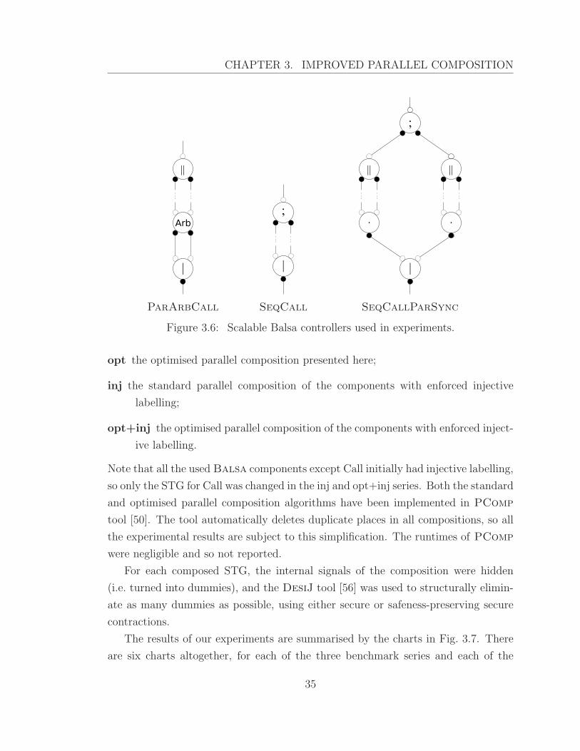
CHAPTER 3. IMPROVED PARALLEL COMPOSITION
||
|
Arb
ParArbCall
;
|
SeqCall
|| ||
;
.
|
.
SeqCallParSync
Figure 3.6: Scalable Balsa controllers used in experiments.
opt the optimised parallel composition presented here;
inj the standard parallel composition of the components with enforced injective
labelling;
opt+inj the optimised parallel composition of the components with enforced inject-
ive labelling.
Note that all the used Balsa components except Call initially had injective labelling,
so only the STG for Call was changed in the inj and opt+inj series. Both the standard
and optimised parallel composition algorithms have been implemented in PComp
tool [50]. The tool automatically deletes duplicate places in all compositions, so all
the experimental results are subject to this simplification. The runtimes of PComp
were negligible and so not reported.
For each composed STG, the internal signals of the composition were hidden
(i.e. turned into dummies), and the DesiJ tool [56] was used to structurally elimin-
ate as many dummies as possible, using either secure or safeness-preserving secure
contractions.
The results of our experiments are summarised by the charts in Fig. 3.7. There
are six charts altogether, for each of the three benchmark series and each of the
35
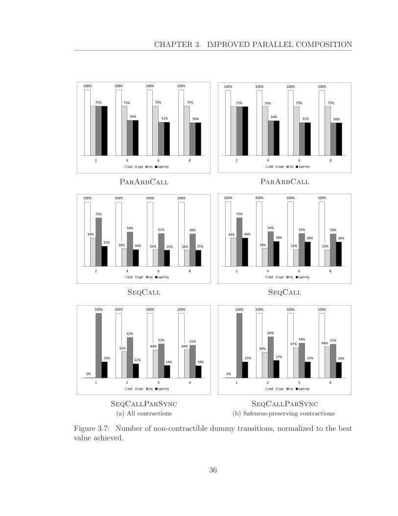
CHAPTER 3. IMPROVED PARALLEL COMPOSITION
100% 100% 100% 100%
75% 75% 75%75%
54%51% 50%
2 4 6 8
std opt inj opt+inj
ParArbCall
100% 100% 100% 100%
44%
28% 26% 25%
75%
54%51% 50%
31%26% 25% 25%
2 4 6 8
std opt inj opt+inj
SeqCall
0%
100% 100% 100%
41%43% 44%
100%
63%
53% 51%
25%22%
19% 19%
1 2 3 4
std opt inj opt+inj
SeqCallParSync
(a) All contractions
100% 100% 100% 100%
75% 75% 75%75%
54%51% 50%
2 4 6 8
std opt inj opt+inj
ParArbCall
100% 100% 100% 100%
44%
28% 26% 25%
75%
54%51% 50%
44%38% 38% 38%
2 4 6 8
std opt inj opt+inj
SeqCall
0%
100% 100% 100%
39%
47% 48%
100%
64%
54% 52%
25% 27% 25% 24%
1 2 3 4
std opt inj opt+inj
SeqCallParSync
(b) Safeness-preserving contractions
Figure 3.7: Number of non-contractible dummy transitions, normalized to the bestvalue achieved.
36
CHAPTER 3. IMPROVED PARALLEL COMPOSITION
contraction modes (secure or safeness-preserving secure). Each chart reports, for
each benchmark size within the corresponding series, the numbers of non-contrac-
tible dummy transitions (normalised w.r.t. the worst result) remaining in the STG
for each of the four composition methods described above.
The experiments demonstrate that the optimised parallel composition is never
worse than the standard one in terms of the STG structure that is used for removing
dummies (the opt bars are never longer than the std bars, and the opt+inj bars
are never longer than the inj bars), and is significantly better in some cases (e.g.
for the SeqCallParSync (4) benchmark there is a factor of five improvement).
Moreover, using the optimised technique in conjunction with injective labelling is
usually advantageous (the fourth bar is the shortest in almost all cases).
3.6 Balsa workflow optimisation through STG re-
synthesis
The main obstacle for the wider acceptance of asynchronous systems is the inherent
complexity of their design. Several solutions are accepted by the industry to help to
simplify the design process through abstraction of predesigned asynchronous circuit
parts as standardised high level components. A designer is able to use these com-
ponents as “building blocks”, and then obtain the final gate-level design through an
automated mapping process. Some of the well-known asynchronous design automa-
tion packages, such as Tangram [8], and Balsa [22], define a high-level programming
language that is used to describe systems. The language constructs are then directly
translated into a network of handshake components– blocks with predefined func-
tionality that use handshakes to interface with other components, which are in turn
mapped into a gate netlist [7].
Although this method greatly enhances the designer’s productivity, it has several
important drawbacks. Of these, the control-path overhead is the most decisive. The
controllers obtained by syntax-directed mapping are usually far from optimal because
the predesigned components are required to implement their declared protocols fully
and correctly in order to be reusable in all possible circuit configurations. However, it
is often the case that a significant part of their functionality becomes redundant due
37
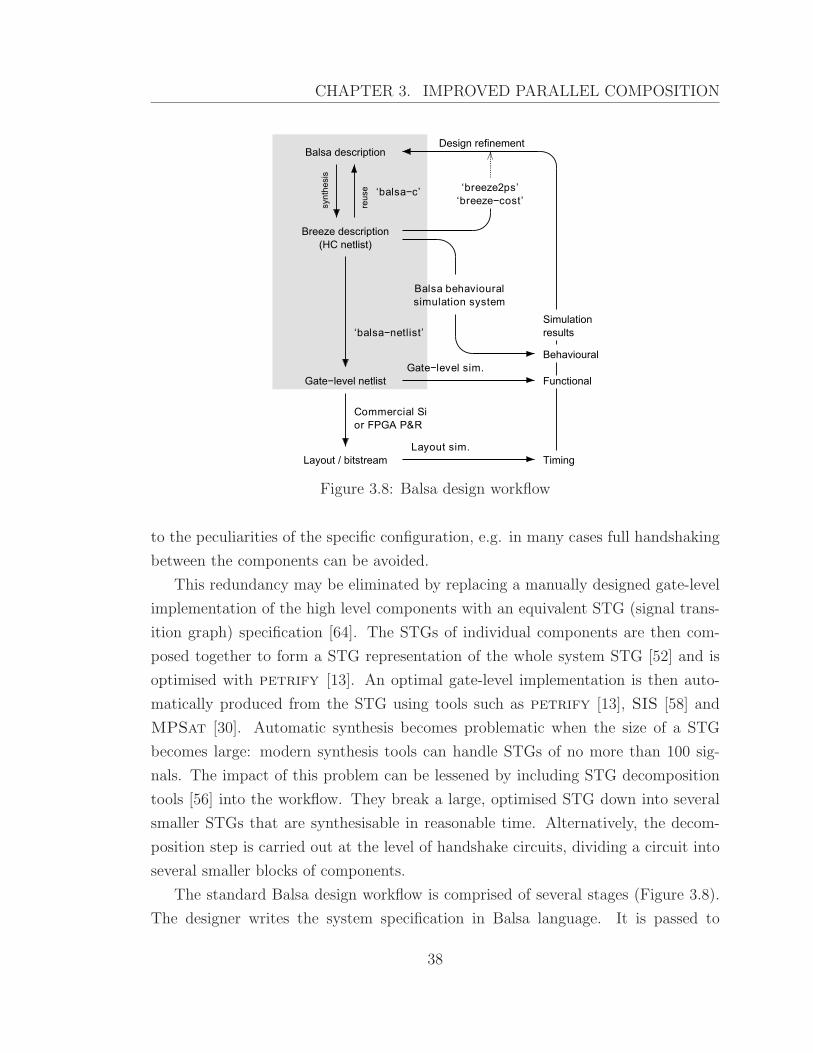
CHAPTER 3. IMPROVED PARALLEL COMPOSITION
Figure 3.8: Balsa design workflow
to the peculiarities of the specific configuration, e.g. in many cases full handshaking
between the components can be avoided.
This redundancy may be eliminated by replacing a manually designed gate-level
implementation of the high level components with an equivalent STG (signal trans-
ition graph) specification [64]. The STGs of individual components are then com-
posed together to form a STG representation of the whole system STG [52] and is
optimised with petrify [13]. An optimal gate-level implementation is then auto-
matically produced from the STG using tools such as petrify [13], SIS [58] and
MPSat [30]. Automatic synthesis becomes problematic when the size of a STG
becomes large: modern synthesis tools can handle STGs of no more than 100 sig-
nals. The impact of this problem can be lessened by including STG decomposition
tools [56] into the workflow. They break a large, optimised STG down into several
smaller STGs that are synthesisable in reasonable time. Alternatively, the decom-
position step is carried out at the level of handshake circuits, dividing a circuit into
several smaller blocks of components.
The standard Balsa design workflow is comprised of several stages (Figure 3.8).
The designer writes the system specification in Balsa language. It is passed to
38
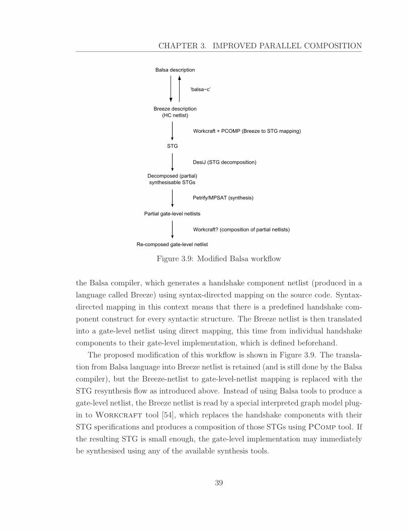
CHAPTER 3. IMPROVED PARALLEL COMPOSITION
Figure 3.9: Modified Balsa workflow
the Balsa compiler, which generates a handshake component netlist (produced in a
language called Breeze) using syntax-directed mapping on the source code. Syntax-
directed mapping in this context means that there is a predefined handshake com-
ponent construct for every syntactic structure. The Breeze netlist is then translated
into a gate-level netlist using direct mapping, this time from individual handshake
components to their gate-level implementation, which is defined beforehand.
The proposed modification of this workflow is shown in Figure 3.9. The transla-
tion from Balsa language into Breeze netlist is retained (and is still done by the Balsa
compiler), but the Breeze-netlist to gate-level-netlist mapping is replaced with the
STG resynthesis flow as introduced above. Instead of using Balsa tools to produce a
gate-level netlist, the Breeze netlist is read by a special interpreted graph model plug-
in to Workcraft tool [54], which replaces the handshake components with their
STG specifications and produces a composition of those STGs using PComp tool. If
the resulting STG is small enough, the gate-level implementation may immediately
be synthesised using any of the available synthesis tools.
39
CHAPTER 3. IMPROVED PARALLEL COMPOSITION
However, for many practical cases the composed STG will become quite large.
In this case, to synthesise the implementation it is necessary to insert an additional
decomposition step, which may be either STG decomposition (implemented using a
tool called DesiJ [56] that is automatically called from the plug-in), or handshake
circuit (HC) decomposition which is supported by the plug-in directly. Therefore,
the whole process is automated in the Workcraft framework.
The technique allows to synthesise more efficient control circuits while at the same
time preserving the benefit of rapid design methodology fundamental to Balsa. It
should be noted, however, that full modelling of all Breeze components with STGs is
not practical. The behaviour of most data components would be too complex to syn-
thesise from an STG. Circuit resynthesis for such components would take too much
time and would often be less effective than an already existing gate-level implement-
ation done by an experienced designer. Subsequently, all data-related functionality
in HCs is modelled outside of STG composition framework: the STG models include
only control signals for the data path elements. These control signals are to be con-
nected after the gate-level generation step to the data-path circuit that is assembled
separately (its components are specified by a structural Verilog netlist). The data
path is generated automatically side-by-side with the STG behaviour model.
3.6.1 Support of Breeze handshake circuits as interpreted
graph model in Workcraft
For the purpose of implementation of the design flow discussed in this section the
Workcraft framework was extended with a plug-in that introduces support for
Breeze HCs. The new HC model allows Workcraft’s convenient visual editing
tools to be applied for creation and editing of Breeze netlists. The same plug-in also
performs generation of the STG behaviour model for the specified HC. The STG
generation algorithm is designed to be highly customisable, with support of multiple
handshake protocols and various STG implementations for each type of component.
At the moment of writing, STG generation was implemented for a limited set of
components using early 4-phase handshake protocol. The library of components is
being expanded and will include all Breeze components with support for different
handshake protocols.
40

CHAPTER 3. IMPROVED PARALLEL COMPOSITION
(a) Sequence
(b) Concur
Figure 3.10: Pure control path handshake components and their respective STGs
3.6.2 STG specifications of individual handshake compon-
ents
Balsa components can be roughly divided in three groups: pure control components,
data path control components and data-control interface components. We will review
each group separately.
Pure control path components
Pure control components only control the behaviour of other components and do
not carry out any data operations. These components are expected to gain the most
from the new design workflow because all of their handshakes are inside the control
path and such handshaking does not have to always strictly correspond to the general
protocol.
The examples are Concur (Figure 3.10b) and SequenceOptimised (Figure 3.10a)
components. The STGs in those figures are highly parallel specifications of these
components. However, experimental results show that although such implementation
might look better on paper, in practise it is sometimes better to specify traditional,
more sequential behaviour. This significantly simplifies the task for synthesis tools,
41
CHAPTER 3. IMPROVED PARALLEL COMPOSITION
particularly those based on state space exploration techniques, because high paral-
lelism often leads to early state space explosion problem. Besides that, a parallel
specification suffers more from CSC (complete state coding) problems: a significant
number of auxiliary signals have to be introduced to achieve CSC.
Data path control components
This group of components is used to control the corresponding data path components
that execute predefined operations on data. These operations are far too complex
for automated synthesis, but the control path part can still be optimised using STG
resynthesis, which makes it reasonable to separate data and control signals. The
signals that control the data path are in this case specified as the input and output
signals of the component’s STG. Because the data path blocks are outside this spe-
cification, their handshake protocols must be implemented strictly and thus cannot
be optimised. This, however, does not prevent the optimisation of handshakes that
belong to the same component but interface with other control path components.
BinaryFunc (Figure 3.11a), CallMux (Figure 3.11b), Variable (Figure 3.11c) are
good examples of the data path control components.
Data-control interface components
Data-control interface components provide conversion of data to control signals or
vice versa. For example, the While component (Figure 3.12a) analyses the input data
to decide whether it should end its operation and conclude the activation handshake,
or to continue activating the output handshake. Case component (Figure 3.12b)
handles the data in a very similar way, however it has an arbitrary bus width, so
for bus widths of more than one bit a decoder that resides in the data path could
be used to reduce the STG complexity. These components STGs can become quite
complex and the strict behaviour of their data-path handshakes must be preserved.
3.6.3 An example: GCD controller
We have chosen the GCD controller (Figure 3.13) to demonstrate the proposed tech-
nique. The GCD controller is a good research example because it has components
42
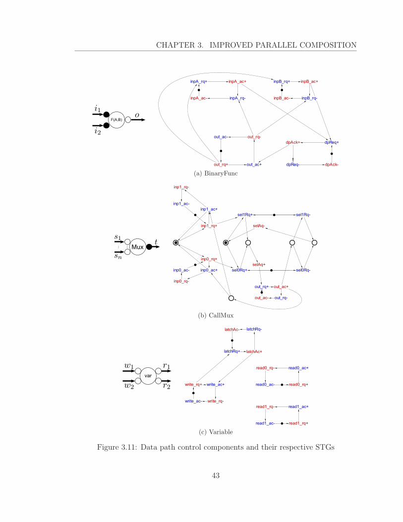
CHAPTER 3. IMPROVED PARALLEL COMPOSITION
(a) BinaryFunc
(b) CallMux
(c) Variable
Figure 3.11: Data path control components and their respective STGs
43

CHAPTER 3. IMPROVED PARALLEL COMPOSITION
(a) While
(b) Case
Figure 3.12: Data-control interface components and their respective STGs
44
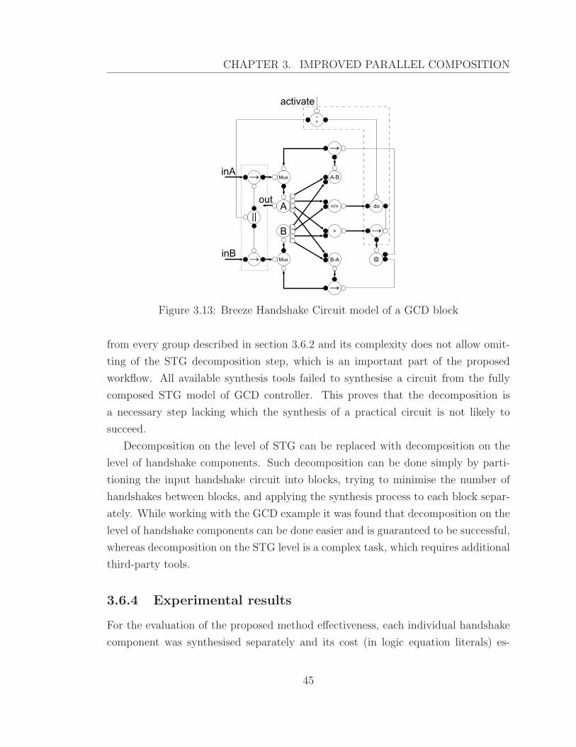
CHAPTER 3. IMPROVED PARALLEL COMPOSITION
Figure 3.13: Breeze Handshake Circuit model of a GCD block
from every group described in section 3.6.2 and its complexity does not allow omit-
ting of the STG decomposition step, which is an important part of the proposed
workflow. All available synthesis tools failed to synthesise a circuit from the fully
composed STG model of GCD controller. This proves that the decomposition is
a necessary step lacking which the synthesis of a practical circuit is not likely to
succeed.
Decomposition on the level of STG can be replaced with decomposition on the
level of handshake components. Such decomposition can be done simply by parti-
tioning the input handshake circuit into blocks, trying to minimise the number of
handshakes between blocks, and applying the synthesis process to each block separ-
ately. While working with the GCD example it was found that decomposition on the
level of handshake components can be done easier and is guaranteed to be successful,
whereas decomposition on the STG level is a complex task, which requires additional
third-party tools.
3.6.4 Experimental results
For the evaluation of the proposed method effectiveness, each individual handshake
component was synthesised separately and its cost (in logic equation literals) es-
45
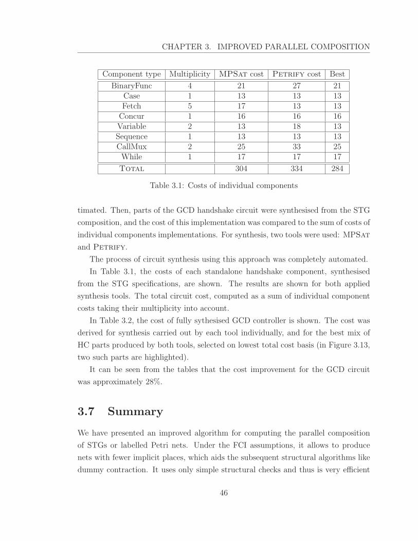
CHAPTER 3. IMPROVED PARALLEL COMPOSITION
Component type Multiplicity MPSat cost Petrify cost Best
BinaryFunc 4 21 27 21Case 1 13 13 13Fetch 5 17 13 13Concur 1 16 16 16Variable 2 13 18 13Sequence 1 13 13 13CallMux 2 25 33 25While 1 17 17 17
Total 304 334 284
Table 3.1: Costs of individual components
timated. Then, parts of the GCD handshake circuit were synthesised from the STG
composition, and the cost of this implementation was compared to the sum of costs of
individual components implementations. For synthesis, two tools were used: MPSat
and Petrify.
The process of circuit synthesis using this approach was completely automated.
In Table 3.1, the costs of each standalone handshake component, synthesised
from the STG specifications, are shown. The results are shown for both applied
synthesis tools. The total circuit cost, computed as a sum of individual component
costs taking their multiplicity into account.
In Table 3.2, the cost of fully sythesised GCD controller is shown. The cost was
derived for synthesis carried out by each tool individually, and for the best mix of
HC parts produced by both tools, selected on lowest total cost basis (in Figure 3.13,
two such parts are highlighted).
It can be seen from the tables that the cost improvement for the GCD circuit
was approximately 28%.
3.7 Summary
We have presented an improved algorithm for computing the parallel composition
of STGs or labelled Petri nets. Under the FCI assumptions, it allows to produce
nets with fewer implicit places, which aids the subsequent structural algorithms like
dummy contraction. It uses only simple structural checks and thus is very efficient
46
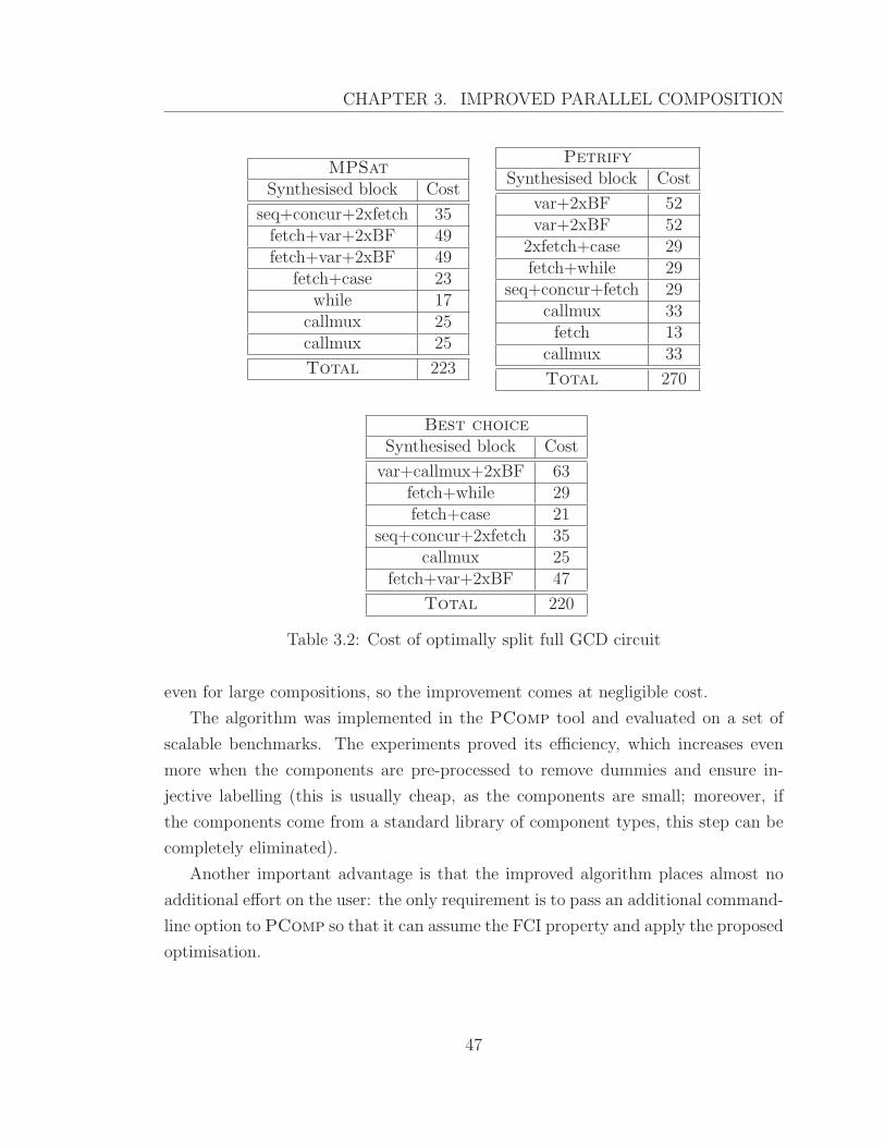
CHAPTER 3. IMPROVED PARALLEL COMPOSITION
MPSat
Synthesised block Cost
seq+concur+2xfetch 35fetch+var+2xBF 49fetch+var+2xBF 49
fetch+case 23while 17
callmux 25callmux 25
Total 223
Petrify
Synthesised block Cost
var+2xBF 52var+2xBF 52
2xfetch+case 29fetch+while 29
seq+concur+fetch 29callmux 33fetch 13
callmux 33
Total 270
Best choice
Synthesised block Cost
var+callmux+2xBF 63fetch+while 29fetch+case 21
seq+concur+2xfetch 35callmux 25
fetch+var+2xBF 47
Total 220
Table 3.2: Cost of optimally split full GCD circuit
even for large compositions, so the improvement comes at negligible cost.
The algorithm was implemented in the PComp tool and evaluated on a set of
scalable benchmarks. The experiments proved its efficiency, which increases even
more when the components are pre-processed to remove dummies and ensure in-
jective labelling (this is usually cheap, as the components are small; moreover, if
the components come from a standard library of component types, this step can be
completely eliminated).
Another important advantage is that the improved algorithm places almost no
additional effort on the user: the only requirement is to pass an additional command-
line option to PComp so that it can assume the FCI property and apply the proposed
optimisation.
47

Chapter 4
Theory of Parametrised Graphs
This chapter is based on the results previously published in [43]. It introduces a new
formalism called Parametrised Graphs (PG) and tries to capture its most important
characteristics in an algebraic structure we call PG-algebra. We introduce some of
the theorems in the theory of PG-algebra and provide their proofs. Many of the
proofs are written in Agda [49], a formal proof language, so they can be machine-
checked instead of being manually inspected.
4.1 Introduction
We continue the work started in [45] where a formal model, called Conditional Partial
Order Graphs (CPOGs), was introduced. Using CPOGs as a foundation allowed us
to represent individual system configurations and operational modes as annotated
graphs and to efficiently overlay them by exploiting their similarities. However,
the CPOG formalism lacks the compositionality and the ability to compare and
transform specifications in a rigorous manner [43]. In particular, CPOGs always
represent a specification as a ‘flat’ structure, similar to the canonical form defined in
Section 4.2, hence a hierarchical representation of a system as a composition of its
components is not possible. We extend this formalism in several ways:
• We transition from the graphs representing partial orders to general graphs
and lift the assumption of graph acyclicity. Nevertheless, if a partial orders is
the most natural way to represent a certain aspect of system, this still can be
48
CHAPTER 4. THEORY OF PARAMETRISED GRAPHS
handled.
• The new formalism is fully compositional – it adds algebraic operations for
combining existing specifications.
• We describe the equivalence relation between the specifications as a set of
axioms, obtaining an algebra of parametrised graphs. This set of axioms is
proved to be sound, minimal and complete [43].
• We have defined equivalence preserving transformations; this permits one to
use the algebra to safely manipulate PG specifications. This can be viewed as
adding a syntactic level to the semantic representation of specifications, and is
reminiscent of the relationship between digital circuits and Boolean algebra.
Since parametrised graphs are likely to be applied in a safety-critical toolchain, it
is imperative to attain a degree of confidence in the properties of the PG formalism.
Equally important is to convince prospective users that the technique is sound and
lives up to its promises. To fulfil this goal, it was decided to construct in a strict
and controlled manner a complete formalisation of the PG formalism. The Agda
system [49] was chosen for its expressive notation language and extensive support
for machine-checked formal inference. Agda has enjoyed a notable success as the
basis for the formalisation of wide range of problems in the domain of programming
language research [5, 27].
We will show that, in contrast to more expressive formalisms such as process al-
gebrae, many useful properties of PGs can be efficiently verified, for example equality
is decidable and, moreover, decidable in NP-time. It therefore lies in the complexity
class below Petri nets (whose interesting properties are PSPACE-hard) and Turing-
powerful process algebrae. Despite their lower expressive power, PGs are sufficient
for our purposes as demonstrated in case studies.
We demonstrate the usefulness of the developed formalism on the basis of two
case studies. The first one (Section 4.5.1) is concerned with development of a phase
encoding controller that represents information by the order of arrival of signals on
n wires. As there are n! possible arrival orders, it is a challenge to specify the set
of corresponding behavioural scenarios in a compact way. The proposed formalism
not only allows us to solve this problem but also does it in a compositional manner.
49

CHAPTER 4. THEORY OF PARAMETRISED GRAPHS
The final specification is obtained through the composition of fixed-size fragments
describing the behaviours of a pair of wires (the latter is impossible with the CPOG
formalism).
4.2 Parametrised Graphs
A Parametrised Graph (PG) is a model which has evolved from Conditional Partial
Order Graphs (CPOG) [45]. We consider directed graphs G = (V,E) whose vertices
are picked from the fixed alphabet of actions A = {a, b, ...}. Hence the vertices of
G would usually model actions (or events) of the system being designed, while the
arcs would usually model the precedence or causality relation: if there is an arc going
from a to b then action a precedes action b. We will denote the empty graph (∅, ∅)
by ε and the singleton graphs ({a}, ∅) simply by a, for any a ∈ A.
Let G1 = (V1, E1) and G2 = (V2, E2) be two graphs, where V1 and V2 as well as
E1 and E2 are not necessarily disjoint. We define the following operations on graphs
(in the order of increasing precedence):
Overlay: G1 +G2df= (V1 ∪ V2, E1 ∪ E2).
Sequence: G1 → G2df= (V1 ∪ V2, E1 ∪ E2 ∪ V1 × V2).
Condition: [1]Gdf= G and [0]G
df= ε.
In other words, the overlay + and sequence → are binary operations on graphs with
the following semantics: G1+G2 is a graph obtained by overlaying graphs G1 and G2,
i.e. it contains the union of their vertices and arcs, while graph G1 → G2 contains
the union plus the arcs connecting every vertex from graph G1 to every vertex from
graph G2 (self-loops can be formed in this way if V1 and V2 are not disjoint). From
the behavioural point of view, if graphs G1 and G2 correspond to two systems then
G1+G2 corresponds to their parallel composition and G1 → G2 corresponds to their
sequential composition. One can observe that any non-empty graph can be obtained
by successively applying the operations + and → to the singleton graphs.
To make notation cleaner we are going to use the following operator precedence
rules: [0] and [1] bind more tightly than → and → binds more tightly than +.
50
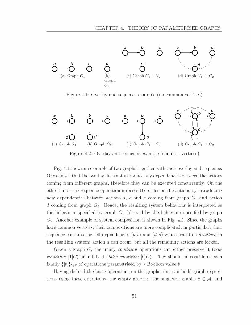
CHAPTER 4. THEORY OF PARAMETRISED GRAPHS
a cb
(a) Graph G1
d
(b)GraphG2
a
�
cb
(c) Graph G1 +G2
a
d
cb
(d) Graph G1 → G2
Figure 4.1: Overlay and sequence example (no common vertices)
d
ba
(a) Graph G1
d
cb
(b) Graph G2
a
d
cb
(c) Graph G1 +G2
a
d
cb
(d) Graph G1 → G2
Figure 4.2: Overlay and sequence example (common vertices)
Fig. 4.1 shows an example of two graphs together with their overlay and sequence.
One can see that the overlay does not introduce any dependencies between the actions
coming from different graphs, therefore they can be executed concurrently. On the
other hand, the sequence operation imposes the order on the actions by introducing
new dependencies between actions a, b and c coming from graph G1 and action
d coming from graph G2. Hence, the resulting system behaviour is interpreted as
the behaviour specified by graph G1 followed by the behaviour specified by graph
G2. Another example of system composition is shown in Fig. 4.2. Since the graphs
have common vertices, their compositions are more complicated, in particular, their
sequence contains the self-dependencies (b, b) and (d, d) which lead to a deadlock in
the resulting system: action a can occur, but all the remaining actions are locked.
Given a graph G, the unary condition operations can either preserve it (true
condition [1]G) or nullify it (false condition [0]G). They should be considered as a
family {[b]}b∈B of operations parametrised by a Boolean value b.
Having defined the basic operations on the graphs, one can build graph expres-
sions using these operations, the empty graph ε, the singleton graphs a ∈ A, and
51
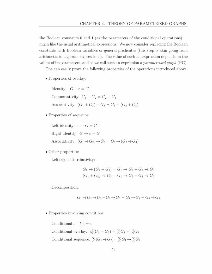
CHAPTER 4. THEORY OF PARAMETRISED GRAPHS
the Boolean constants 0 and 1 (as the parameters of the conditional operations) —
much like the usual arithmetical expressions. We now consider replacing the Boolean
constants with Boolean variables or general predicates (this step is akin going from
arithmetic to algebraic expressions). The value of such an expression depends on the
values of its parameters, and so we call such an expression a parametrised graph (PG).
One can easily prove the following properties of the operations introduced above.
• Properties of overlay:
Identity: G+ ε = G
Commutativity: G1 +G2 = G2 +G1
Associativity: (G1 +G2) +G3 = G1 + (G2 +G3)
• Properties of sequence:
Left identity: ε→ G = G
Right identity: G→ ε = G
Associativity: (G1→G2)→G3 = G1→(G2→G3)
• Other properties:
Left/right distributivity:
G1 → (G2 +G3) = G1 → G2 +G1 → G3
(G1 +G2) → G3 = G1 → G3 +G2 → G3
Decomposition:
G1→G2→G3=G1→G2 +G1→G3 +G2→G3
• Properties involving conditions:
Conditional ε: [b]ε = ε
Conditional overlay: [b](G1 +G2) = [b]G1 + [b]G2
Conditional sequence: [b](G1→G2)=[b]G1→ [b]G2
52
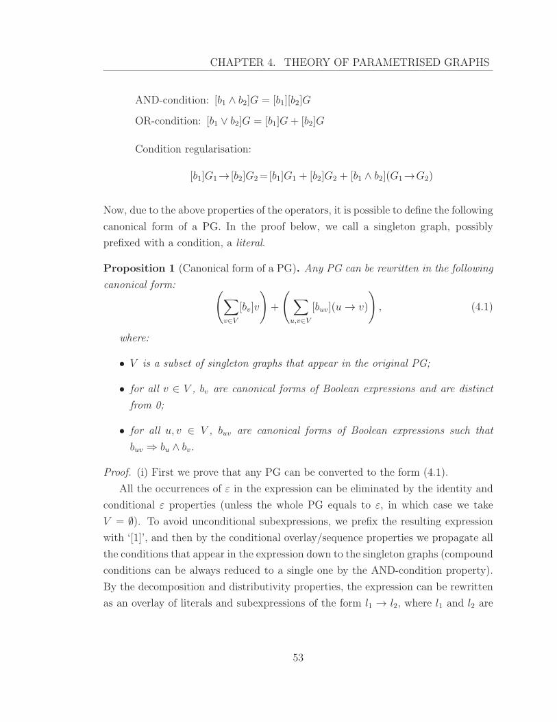
CHAPTER 4. THEORY OF PARAMETRISED GRAPHS
AND-condition: [b1 ∧ b2]G = [b1][b2]G
OR-condition: [b1 ∨ b2]G = [b1]G+ [b2]G
Condition regularisation:
[b1]G1→ [b2]G2=[b1]G1 + [b2]G2 + [b1 ∧ b2](G1→G2)
Now, due to the above properties of the operators, it is possible to define the following
canonical form of a PG. In the proof below, we call a singleton graph, possibly
prefixed with a condition, a literal.
Proposition 1 (Canonical form of a PG). Any PG can be rewritten in the following
canonical form:(
∑
v∈V
[bv]v
)
+
(
∑
u,v∈V
[buv](u→ v)
)
, (4.1)
where:
• V is a subset of singleton graphs that appear in the original PG;
• for all v ∈ V , bv are canonical forms of Boolean expressions and are distinct
from 0;
• for all u, v ∈ V , buv are canonical forms of Boolean expressions such that
buv ⇒ bu ∧ bv.
Proof. (i) First we prove that any PG can be converted to the form (4.1).
All the occurrences of ε in the expression can be eliminated by the identity and
conditional ε properties (unless the whole PG equals to ε, in which case we take
V = ∅). To avoid unconditional subexpressions, we prefix the resulting expression
with ‘[1]’, and then by the conditional overlay/sequence properties we propagate all
the conditions that appear in the expression down to the singleton graphs (compound
conditions can be always reduced to a single one by the AND-condition property).
By the decomposition and distributivity properties, the expression can be rewritten
as an overlay of literals and subexpressions of the form l1 → l2, where l1 and l2 are
53
CHAPTER 4. THEORY OF PARAMETRISED GRAPHS
literals. The latter subexpressions can be rewritten using the condition regularisation
rule:
[b1]u→ [b2]v = [b1]u+ [b2]v + [b1 ∧ b2](u→ v)
Now, literals corresponding to the same singleton graphs, as well as subexpressions
of the form [b](u → v) that correspond to the same pair of singleton graphs u
and v, are combined using the OR-condition property. Then the literals prefixed
with 0 conditions can be dropped. Now the set V consists of all the singleton graphs
occurring in the literals. To turn the overall expression into the required form it only
remains to add missing subexpressions of the form [0](u→ v) for every u, v ∈ V such
that the expression does not contain the subexpression of the form [b](u→ v). Note
that the property buv ⇒ bu ∧ bv is always enforced by this construction:
• condition regularisation ensures this property;
• combining literals using the OR-condition property can only strengthen the
right hand side of this implication, and so cannot violate it;
• adding [0](u → v) does not violate the property as it trivially holds when
buv = 0.
(ii) We now show that (4.1) is a canonical form, i.e. if L = R then their canonical
forms can(L) and can(R) coincide.
For the sake of contradiction, assume this is not the case. Then we consider two
cases (all possible cases are symmetric to one of these two):
1. can(L) contains a literal [bv]v whereas can(R) either contains a literal [b′v]v
with b′v 6≡ bv or does not contain any literal corresponding to v, in which case
we say that it contains a literal [b′v]v with b′v = 0. Then for some values of
parameters one of the graphs will contain vertex v while the other will not.
2. can(L) and can(R) have the same set V of vertices, but can(L) contains a
subexpression [buv](u→ v) whereas can(R) contains a subexpression [b′uv](u→
v) with b′uv 6≡ buv. Then for some values of parameters one of the graphs will
contain the arc (u, v) (note that due to buv ⇒ bu∧ bv and b′uv ⇒ bu∧ bv vertices
u and v are present), while the other will not.
54
CHAPTER 4. THEORY OF PARAMETRISED GRAPHS
In both cases there is a contradiction with L = R.
This canonical form allows one to lift the notion of adjacency matrix of a graph to
PGs. Recall that the adjacency matrix (buv) of a graph (V,E) is a |V |× |V | Boolean
matrix such that buv = 1 if (u, v) ∈ E and buv = 0 otherwise. The adjacency matrix
of a PG is obtained from the canonical form (4.1) by gathering the predicates buv
into a matrix. The adjacency matrix of a PG is similar to that of a graph, but it
contains predicates rather than Boolean values. It does not uniquely determine a
PG, as the predicates of the vertices cannot be derived from it; to fully specify a PG
one also has to provide predicates bv from the canonical form (4.1).
Another advantage of this canonical form is that it provides a graphical notation
for PGs. The vertices occurring in the canonical form (set V ) can be represented
by circles, and the subexpressions of the form u → v by arcs. The label of a vertex
v consists of the vertex name, colon and the predicate bv, while every arc (u, v) is
labelled with the corresponding predicate buv. As adjacency matrices of PGs tend
to have many constant elements, we use a simplified notation in which the arcs
with constant 0 predicates are not drawn, and constant 1 predicates are dropped;
moreover, it is convenient to assume that the predicates on arcs are implicitly ANDed
with those on incident vertices (to enforce the invariant buv ⇒ bu ∧ bv), which often
allows one to simplify predicates on arcs. This can be justified by introducing the
ternary operator, called conditional sequence:
ub
−→ vdf= [b](u→ v) + u+ v
Intuitively, PG ub
−→ v consists of two unconditional vertices connected by an arc
with the condition b. By case analysis on b1 and b2 one can easily prove the following
properties of the conditional sequence that allow simplifying the predicates on arcs:
[b1]ub1∧b2−−−→ v = [b1]u
b2−→ v
ub1∧b2−−−→ [b2]v = u
b1−→ [b2]v
Fig. 4.3(top) shows an example of a PG. The predicates depend on a Boolean
variable x. The predicates of vertices a, b and d are constants 1; such vertices are
called unconditional. Vertices c and e are conditional, and their predicates are x
55
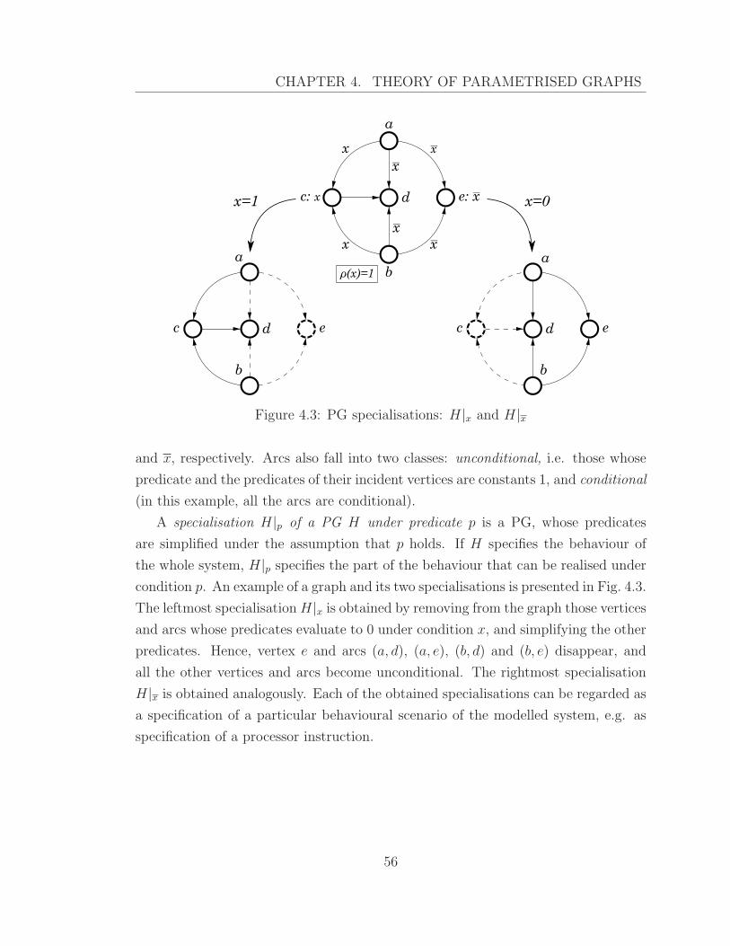
CHAPTER 4. THEORY OF PARAMETRISED GRAPHS
a
d
b
c: x e: x_
x
x
x _
x _
ρ(x)=1
a
d
b
c e
x=1
a
d
b
c e
x=0
x _
x _
Figure 4.3: PG specialisations: H|x and H|x
and x, respectively. Arcs also fall into two classes: unconditional, i.e. those whose
predicate and the predicates of their incident vertices are constants 1, and conditional
(in this example, all the arcs are conditional).
A specialisation H|p of a PG H under predicate p is a PG, whose predicates
are simplified under the assumption that p holds. If H specifies the behaviour of
the whole system, H|p specifies the part of the behaviour that can be realised under
condition p. An example of a graph and its two specialisations is presented in Fig. 4.3.
The leftmost specialisationH|x is obtained by removing from the graph those vertices
and arcs whose predicates evaluate to 0 under condition x, and simplifying the other
predicates. Hence, vertex e and arcs (a, d), (a, e), (b, d) and (b, e) disappear, and
all the other vertices and arcs become unconditional. The rightmost specialisation
H|x is obtained analogously. Each of the obtained specialisations can be regarded as
a specification of a particular behavioural scenario of the modelled system, e.g. as
specification of a processor instruction.
56
CHAPTER 4. THEORY OF PARAMETRISED GRAPHS
4.2.1 Specification and composition of instructions
Consider a processing unit that has two registers A and B, and can perform two
different instructions: addition and exchange of two variables stored in memory. The
processor contains five datapath components (denoted by a . . . e) that can perform
the following atomic actions:
a) Load register A from memory;
b) Load register B from memory;
c) Compute the sum of the numbers stored in registers A and B, and store it in
A;
d) Save register A into memory;
e) Save register B into memory.
Table 4.1 describes the addition and exchange instructions in terms of usage of these
atomic actions.
The addition instruction consists of loading the two operands from memory (caus-
ally independent actions a and b), their addition (action c), and saving the result
(action d). Let us assume for simplicity that in this example all causally independent
actions are always performed concurrently, see the corresponding scenario ADD in
the table.
The operation of exchange consists of loading the operands (causally independent
actions a and b), and saving them into swapped memory locations (causally inde-
pendent actions d and e), as captured by the XCHG scenario. Note that in order to
start saving one of the registers it is necessary to wait until both of them have been
loaded to avoid overwriting one of the values.
One can see that the two scenarios in Table 4.1 appear to be the two special-
isations of the PG shown in Fig. 4.3, thus this PG can be considered as a joint
specification of both instructions. Two important characteristics of such a specifica-
tion are that the common events {a, b, d} are overlaid, and the choice between the two
operations is modelled by the Boolean predicates associated with the vertices and
arcs of the PG. As a result, in our model there is no need for a ‘nodal point’ of choice,
which tend to appear in alternative specification models: a Petri Net (resp. Finite
57
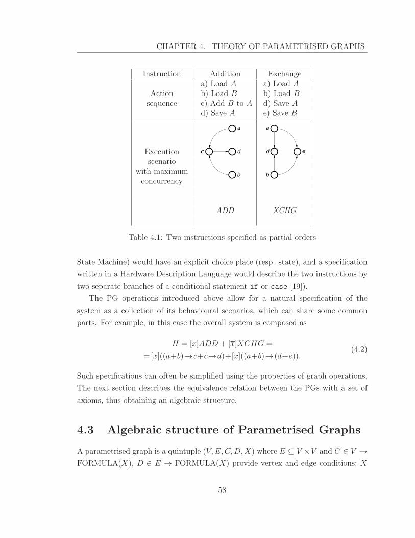
CHAPTER 4. THEORY OF PARAMETRISED GRAPHS
Instruction Addition Exchangea) Load A a) Load A
Action b) Load B b) Load Bsequence c) Add B to A d) Save A
d) Save A e) Save B
Execution
a
d
b
�
a
d
b
e
scenariowith maximumconcurrency
ADD XCHG
Table 4.1: Two instructions specified as partial orders
State Machine) would have an explicit choice place (resp. state), and a specification
written in a Hardware Description Language would describe the two instructions by
two separate branches of a conditional statement if or case [19]).
The PG operations introduced above allow for a natural specification of the
system as a collection of its behavioural scenarios, which can share some common
parts. For example, in this case the overall system is composed as
H = [x]ADD + [x]XCHG =
=[x]((a+b)→c+c→d)+[x]((a+b)→(d+e)).(4.2)
Such specifications can often be simplified using the properties of graph operations.
The next section describes the equivalence relation between the PGs with a set of
axioms, thus obtaining an algebraic structure.
4.3 Algebraic structure of Parametrised Graphs
A parametrised graph is a quintuple (V,E,C,D,X) where E ⊆ V ×V and C ∈ V →
FORMULA(X), D ∈ E → FORMULA(X) provide vertex and edge conditions; X
58
CHAPTER 4. THEORY OF PARAMETRISED GRAPHS
is the set of identifiers occuring free in parametrisation conditions. Some ϕ from
FORMULA(X) is a Boolean predicate with free variables from X. We consider a
predicate equal to another predicate whenever they are extensionally equal. For any
x ∈ X, we say that the formula x ∈ FORMULA(X) is an atomic occurrence of x.
A PG-algebra is a tuple 〈G,+,→, [0], [1]〉, where G is a set of graphs whose vertices
are picked from the alphabet A and the operations match those defined for graphs
above. The equivalence relation is given by the following axioms.
• + is commutative and associative
• → is associative
• ε is a left and right identity of →
• → distributes over +:
p→ (q + r) = p→ q + p→ r
(p+ q) → r = p→ r + q → r
• Decomposition:p→ q → r = p→ q + p→ r + q → r
• Condition: [0]p = ε and [1]p = p
The following derived equalities can be proved from PG-algebra axioms [42, Prop.
2, 3]:
• ε is an identity of +: p+ ε = p
• + is idempotent: p+ p = p
• Left and right absorption:
p+ p→ q = p→ q
q + p→ q = p→ q
• Conditional ε: [b]ε = ε
• Conditional overlay: [b](p+ q) = [b]p+ [b]q
59
CHAPTER 4. THEORY OF PARAMETRISED GRAPHS
• Conditional sequence: [b](p→ q) = [b]p→ [b]q
• AND-condition: [b1 ∧ b2]p = [b1][b2]p
• OR-condition: [b1 ∨ b2]p = [b1]p+ [b2]p
• Choice propagation:
[b](p→ q) + [b](p→ r) = p→ ([b]q + [b]r)
[b](p→ r) + [b](q → r) = ([b]p+ [b]q) → r
• Condition regularisation:
[b1]p→ [b2]q = [b1]p+ [b2]q + [b1 ∧ b2](p→ q)
Note that as ε is a left and right identity of → and +, there can be no other identities
for these operations. Interestingly, unlike with many other algebraic structures, the
two main operations in the PG-algebra have the same identity.
It is easy to see that PGs are a model of PG-algebra, as all the axioms of PG-
algebra are satisfied by PGs; in particular, this means that PG-algebra is sound.
Moreover, any PG-algebra expression has the canonical form (4.1), as the proof of
Prop. 1 can be directly imported:
• It is always possible to translate a PG-algebra expression to this canonical form,
as part (i) of the proof relies only on the properties of PGs that correspond to
either PG-algebra axioms or equalities above.
• If L = R holds in PG-algebra then L = R holds also for PGs (as PGs are a
model of PG-algebra), and so the PGs can(L) and can(R) coincide, see part (ii)
of the proof. Since PGs can(L) and can(R) are in fact the same objects as the
expressions can(L) and can(R) of the PG-algebra, (4.1) is a canonical form of
a PG-algebra expression.
This also means that PG-algebra is complete w.r.t. PGs, i.e. any PG equality can
be either proved or disproved using the axioms of PG-algebra (by converting to the
canonical form).
60

CHAPTER 4. THEORY OF PARAMETRISED GRAPHS
[x]((a+ b) → c+ c→ d) + [x]((a+ b) → (d+ e)) = (closure)
[x]((a+ b) → c+ (a+ b) → d+ c→ d) +
+[x]((a+ b) → (d+ e)) = (decomposition)
[x]((a+ b) → c→ d) + [x]((a+ b) → (d+ e)) = (choice propagation)
(a+ b) → ([x](c→ d) + [x](d+ e)) = (conditional overlay)
(a+ b) → ([x](c→ d) + [x]d+ [x]e) = (→ −identity)
(a+ b) → ([x](c→ d) + [x](ε→ d) + [x]e) = (choice propagation)
(a+ b) → (([x]c+ [x]ε) → d+ [x]e) = (conditional ε, +-identity)
(a+ b) → ([x]c→ d+ [x]e).
Figure 4.4: Simplifying expression (4.2) using the Closure axiom
The provided set of axioms of PG-algebra is minimal, i.e. no axiom from this
set can be derived from the others. The minimality was checked by enumerating the
fixed-size models of PG-algebra with the help of the Alg tool [9]: It turns out that
removing any of the axioms leads to a different number of non-isomorphic models of
a particular size, implying that all the axioms are necessary.
Hence, the following result holds:
Theorem 2 (Soundness, Minimality and Completeness). The set of axioms of PG-
algebra is sound, minimal and complete w.r.t. PGs.
4.4 Transitive Parametrised Graphs and their al-
gebra
In many cases the arcs of the graphs are interpreted as the causality relation, and so
the graph itself is a partial order. However, in practice it is convenient to drop some
or all of the transitive arcs, i.e. two graphs should be considered equal whenever their
transitive closures are equal. E.g. in this case the graphs specified by the expressions
a → b + b → c and a → b + a → c + b → c are considered as equal. PGs with this
equality relation are called Transitive Parametrised Graphs (TPG). To capture this
61
CHAPTER 4. THEORY OF PARAMETRISED GRAPHS
algebraically, we augment the PG-algebra with the Closure axiom:
if q 6= ε then p→q + q→r = p→q + p→r + q→r.
One can see that by repeated application of this axiom one can obtain the transitive
closure of any graph, including those with cycles. The resulting algebraic structure
is called Transitive Parametrised Graphs Algebra (TPG-algebra).
Note that the condition q 6= ε in the Closure axiom is necessary, as otherwise
a+ b = a→ε+ ε→b = a→ε+ a→b+ ε→b = a→b,
and the operations + and → become identical, which is clearly undesirable.
The Closure axiom helps to simplify specifications by reducing the number of arcs
and/or simplifying their conditions. For example, consider the PG expression (4.2).
As the scenarios of this PG are interpreted as the orders of execution of actions, it
is natural to use the Closure axiom. Note that the expression cannot be simplified
in PG-algebra; however, in the TPG-algebra it can be considerably simplified, as
shown in Fig. 4.4.
The corresponding TPG is shown in Fig. 4.5. Note that it has fewer conditional
elements than the PG in Fig. 4.3; though the specialisations are now different, they
have the same transitive closures.
We now lift the canonical form (4.1) to TPGs and TPG-algebra. Note that the
only difference is the last requirement.
Proposition 3 (Canonical form of a TPG). Any TPG can be rewritten in the fol-
lowing canonical form:
(
∑
v∈V
[bv]v
)
+
(
∑
u,v∈V
[buv](u→ v)
)
, (4.3)
where:
1. V is a subset of singleton graphs that appear in the original TPG;
2. for all v ∈ V , bv are canonical forms of Boolean expressions and are distinct
from 0;
62
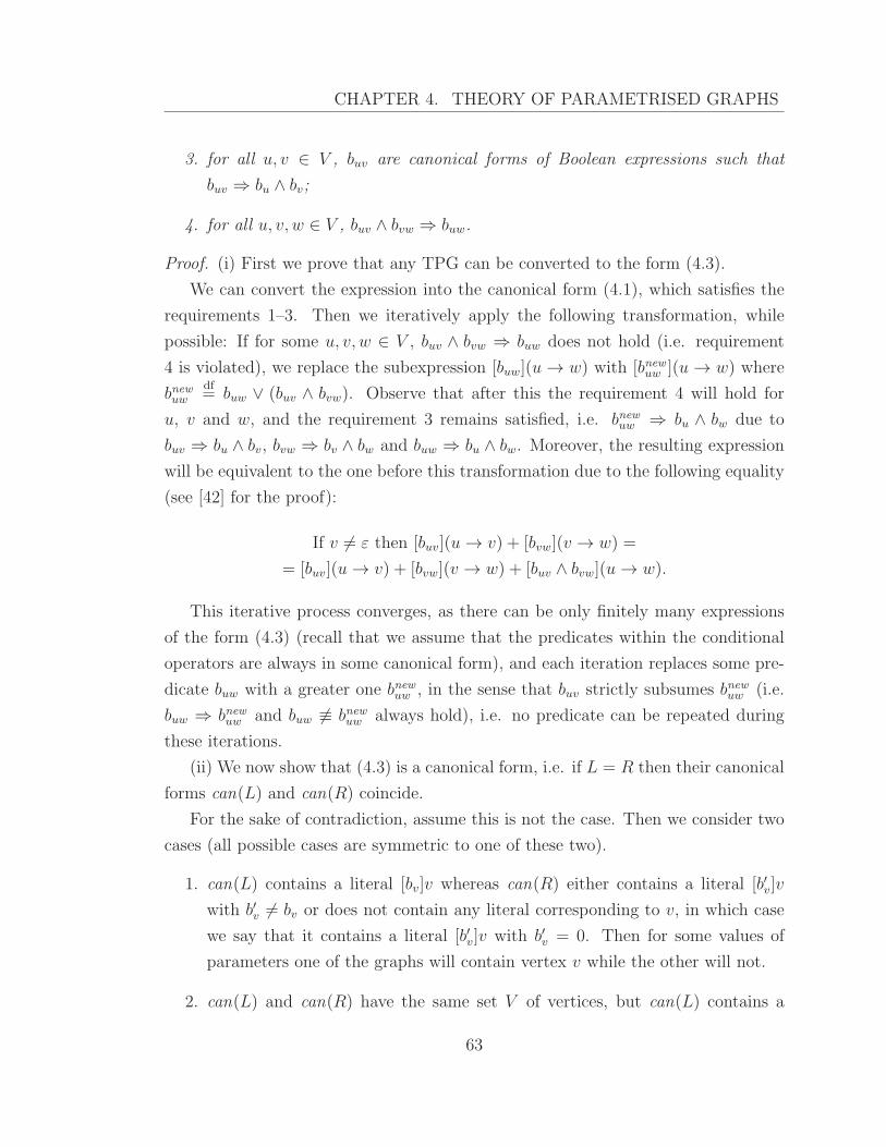
CHAPTER 4. THEORY OF PARAMETRISED GRAPHS
3. for all u, v ∈ V , buv are canonical forms of Boolean expressions such that
buv ⇒ bu ∧ bv;
4. for all u, v, w ∈ V , buv ∧ bvw ⇒ buw.
Proof. (i) First we prove that any TPG can be converted to the form (4.3).
We can convert the expression into the canonical form (4.1), which satisfies the
requirements 1–3. Then we iteratively apply the following transformation, while
possible: If for some u, v, w ∈ V , buv ∧ bvw ⇒ buw does not hold (i.e. requirement
4 is violated), we replace the subexpression [buw](u → w) with [bnewuw ](u → w) where
bnewuwdf= buw ∨ (buv ∧ bvw). Observe that after this the requirement 4 will hold for
u, v and w, and the requirement 3 remains satisfied, i.e. bnewuw ⇒ bu ∧ bw due to
buv ⇒ bu ∧ bv, bvw ⇒ bv ∧ bw and buw ⇒ bu ∧ bw. Moreover, the resulting expression
will be equivalent to the one before this transformation due to the following equality
(see [42] for the proof):
If v 6= ε then [buv](u→ v) + [bvw](v → w) =
= [buv](u→ v) + [bvw](v → w) + [buv ∧ bvw](u→ w).
This iterative process converges, as there can be only finitely many expressions
of the form (4.3) (recall that we assume that the predicates within the conditional
operators are always in some canonical form), and each iteration replaces some pre-
dicate buw with a greater one bnewuw , in the sense that buv strictly subsumes bnewuw (i.e.
buw ⇒ bnewuw and buw 6≡ bnewuw always hold), i.e. no predicate can be repeated during
these iterations.
(ii) We now show that (4.3) is a canonical form, i.e. if L = R then their canonical
forms can(L) and can(R) coincide.
For the sake of contradiction, assume this is not the case. Then we consider two
cases (all possible cases are symmetric to one of these two).
1. can(L) contains a literal [bv]v whereas can(R) either contains a literal [b′v]v
with b′v 6= bv or does not contain any literal corresponding to v, in which case
we say that it contains a literal [b′v]v with b′v = 0. Then for some values of
parameters one of the graphs will contain vertex v while the other will not.
2. can(L) and can(R) have the same set V of vertices, but can(L) contains a
63
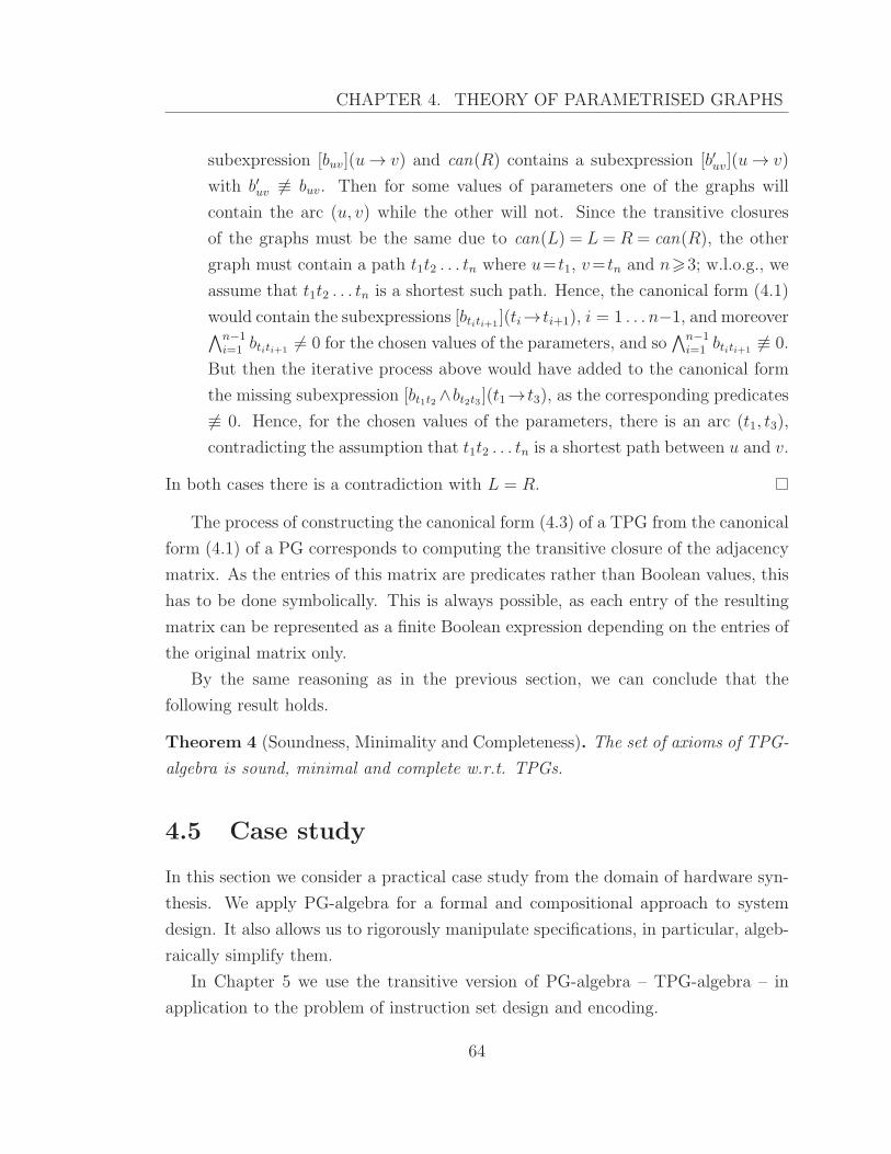
CHAPTER 4. THEORY OF PARAMETRISED GRAPHS
subexpression [buv](u→ v) and can(R) contains a subexpression [b′uv](u→ v)
with b′uv 6≡ buv. Then for some values of parameters one of the graphs will
contain the arc (u, v) while the other will not. Since the transitive closures
of the graphs must be the same due to can(L) = L = R = can(R), the other
graph must contain a path t1t2 . . . tn where u= t1, v= tn and n>3; w.l.o.g., we
assume that t1t2 . . . tn is a shortest such path. Hence, the canonical form (4.1)
would contain the subexpressions [btiti+1](ti→ ti+1), i = 1 . . . n−1, and moreover
∧n−1i=1 btiti+1
6= 0 for the chosen values of the parameters, and so∧n−1
i=1 btiti+16≡ 0.
But then the iterative process above would have added to the canonical form
the missing subexpression [bt1t2 ∧bt2t3 ](t1→ t3), as the corresponding predicates
6≡ 0. Hence, for the chosen values of the parameters, there is an arc (t1, t3),
contradicting the assumption that t1t2 . . . tn is a shortest path between u and v.
In both cases there is a contradiction with L = R.
The process of constructing the canonical form (4.3) of a TPG from the canonical
form (4.1) of a PG corresponds to computing the transitive closure of the adjacency
matrix. As the entries of this matrix are predicates rather than Boolean values, this
has to be done symbolically. This is always possible, as each entry of the resulting
matrix can be represented as a finite Boolean expression depending on the entries of
the original matrix only.
By the same reasoning as in the previous section, we can conclude that the
following result holds.
Theorem 4 (Soundness, Minimality and Completeness). The set of axioms of TPG-
algebra is sound, minimal and complete w.r.t. TPGs.
4.5 Case study
In this section we consider a practical case study from the domain of hardware syn-
thesis. We apply PG-algebra for a formal and compositional approach to system
design. It also allows us to rigorously manipulate specifications, in particular, algeb-
raically simplify them.
In Chapter 5 we use the transitive version of PG-algebra – TPG-algebra – in
application to the problem of instruction set design and encoding.
64
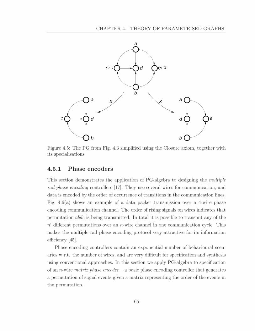
CHAPTER 4. THEORY OF PARAMETRISED GRAPHS
a
d
b
�_
a
d
b
a
d
b
x x_
Figure 4.5: The PG from Fig. 4.3 simplified using the Closure axiom, together withits specialisations
4.5.1 Phase encoders
This section demonstrates the application of PG-algebra to designing the multiple
rail phase encoding controllers [17]. They use several wires for communication, and
data is encoded by the order of occurrence of transitions in the communication lines.
Fig. 4.6(a) shows an example of a data packet transmission over a 4-wire phase
encoding communication channel. The order of rising signals on wires indicates that
permutation abdc is being transmitted. In total it is possible to transmit any of the
n! different permutations over an n-wire channel in one communication cycle. This
makes the multiple rail phase encoding protocol very attractive for its information
efficiency [45].
Phase encoding controllers contain an exponential number of behavioural scen-
arios w.r.t. the number of wires, and are very difficult for specification and synthesis
using conventional approaches. In this section we apply PG-algebra to specification
of an n-wire matrix phase encoder – a basic phase encoding controller that generates
a permutation of signal events given a matrix representing the order of the events in
the permutation.
65
CHAPTER 4. THEORY OF PARAMETRISED GRAPHS
a
b
c
�
(a) Phase encoded data
Matrix
phase
encoder
v1v2
vn
x12x21x13x31
x(n-1)nxn(n-1)
......
(b) Matrix phase encoder
Figure 4.6: Multiple rail phase encoding
Fig. 4.6(b) shows the top-level view of the controller’s structure. Its inputs are(
n2
)
dual-rail ports that specify the order of signals to be produced at the controller’s
n output wires. The inputs of the controller can be viewed as an n × n Boolean
matrix (xij) with diagonal elements being 0. The outputs of the controller will be
modelled by n actions vi ∈ A. Whenever xij = 1, event vi must happen before
event vj. It is guaranteed that xij and xji cannot be 1 at the same time, however,
they can be simultaneously 0, meaning that the relative order of the events is not
known yet and the controller has to wait until xij = 1 or xji = 1 is satisfied (other
outputs for which the order is already known can be generated meanwhile).
The overall specification of the controller is obtained as the overlay∑
1≤i<j≤n
Hij of
fixed-size expressions Hij, modelling the behaviour of each pair of outputs. In turn,
each Hij is an overlay of three possible scenarios:
1. If xij = 1 (and so xji = 0) then there is a causal dependency between vi and
vj, described using the PG-algebra sequence operator: vi → vj.
2. If xji = 1 (and so xij = 0) then there is a causal dependency between vj and
vi: vj → vi.
3. If xij = xji = 0 then neither vi nor vj can be produced yet; this is expressed
by a circular wait condition between vi and vj: vi → vj + vj → vi.1
We prefix each of the scenarios with its precondition and overlay the results:
Hij = [xij ∧ xji](vi → vj) + [xji ∧ xij ](vj → vi)+
+[xij ∧ xji](vi → vj + vj → vi).
1There are other ways to describe this scenario, e.g. by creating self-loops vi → vi + vj → vj .
66
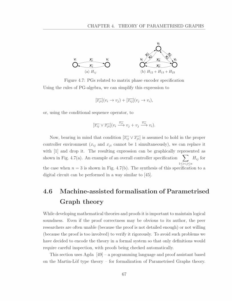
CHAPTER 4. THEORY OF PARAMETRISED GRAPHS
vi vjxj i
_
xi j
_
(a) Hij
v1
v2
v3x31_
x13_
x21_
x12_x32
_
x23
_
(b) H12 +H13 +H23
Figure 4.7: PGs related to matrix phase encoder specification
Using the rules of PG-algebra, we can simplify this expression to
[xji](vi → vj) + [xij](vj → vi),
or, using the conditional sequence operator, to
[xij ∨ xji](vixji
−→ vj + vjxij
−→ vi).
Now, bearing in mind that condition [xij ∨ xji] is assumed to hold in the proper
controller environment (xij and xji cannot be 1 simultaneously), we can replace it
with [1] and drop it. The resulting expression can be graphically represented as
shown in Fig. 4.7(a). An example of an overall controller specification∑
1≤i<j≤n
Hij for
the case when n = 3 is shown in Fig. 4.7(b). The synthesis of this specification to a
digital circuit can be performed in a way similar to [45].
4.6 Machine-assisted formalisation of Parametrised
Graph theory
While developing mathematical theories and proofs it is important to maintain logical
soundness. Even if the proof correctness may be obvious to its author, the peer
researchers are often unable (because the proof is not detailed enough) or not willing
(because the proof is too involved) to verify it rigorously. To avoid such problems we
have decided to encode the theory in a formal system so that only definitions would
require careful inspection, with proofs being checked automatically.
This section uses Agda [49] – a programming language and proof assistant based
on the Martin-Lof type theory – for formalization of Parametrised Graphs theory.
67
CHAPTER 4. THEORY OF PARAMETRISED GRAPHS
The section additionally describes the algorithm for conversion of PG formulae to
normal form and shows that the correctness of the algorithm has been verified.
The section extensively uses the syntax of Agda and references several definitions
from the Agda standard library [18].
4.6.1 Graph Algebra
We start with defining an algebraic structure of non-parametrised graphs, to extend
them with conditions later.
We define graph algebra as an algebraic structure over a set G with an equivalence
relation ≈ supporting the following operations:
• An empty graph, denoting no actions.
ε : G
• Graph overlay, denoting the parallel composition of actions from both graphs.
+ : G → G → G
• Graph sequencing, denoting the causal dependency between actions in the first
graph and in the second graph.
≫ : G → G → G
Additionally, the operations must satisfy the following properties:
• Overlay is commutative and associative.
+assoc : ∀ p q r → (p + q) + r ≈ p + (q + r)
+comm : ∀ p q → p + q ≈ q + p
• Sequencing is associative.
≫ assoc : ∀ p q r →
(p ≫ q) ≫ r ≈ p ≫ (q ≫ r)
68
CHAPTER 4. THEORY OF PARAMETRISED GRAPHS
• Empty graph is a no-op in relation to sequencing.
≫ identityl : ∀ p → ε≫ p ≈ p
≫ identityr : ∀ p → p ≫ ε ≈ p
• Sequencing distributes over overlay.
distribl : ∀ p q r →
p ≫ (q + r) ≈ p ≫ q + p ≫ r
distribr : ∀ p q r →
(p + q) ≫ r ≈ p ≫ r + q ≫ r
• Sequence of more than two actions may be decomposed into shorter sequences,
forming the original sequence with overlay.
decomposition : ∀ p q r →
p ≫ q ≫ r ≈ p ≫ q + p ≫ r + q ≫ r
Derived theorems
The following theorems has been derived from the axioms:
• Empty graph is a no-op in relation to overlay.
+identity : ∀ p → p + ε ≈ p
• Overlay is idempotent.
+idempotence : ∀ p → p + p ≈ p
• Absorption.
absorptionl : ∀ p q → p ≫ q + p ≈ p ≫ q
absorptionr : ∀ p q → p ≫ q + q ≈ p ≫ q
69
CHAPTER 4. THEORY OF PARAMETRISED GRAPHS
4.6.2 Parametrised Graphs
The graph algebra introduced in the previous subsection can only describe static
event dependencies. To describe complex dynamic systems one has to consider the
conditional behaviour as well. To do this, we have extended the graph algebra by
annotating the graphs with conditions. Given a set G of the parametrised graphs and
a set B of all the possible Boolean conditions, together with the following operations:
∨ : B → B → B
∧ : B → B → B
¬ : B → B
⊤ : B
⊥ : B
we require a new operation called condition:
[ ] : B → G → G
The condition operation must have the following properties:
true-condition : ∀ x → [⊤] x ≈ x
false-condition : ∀ x → [⊥] x ≈ ε
and-condition : ∀ f g x → [f ∧ g ] x ≈ [f ] [g ] x
or-condition : ∀ f g x → [f ∨ g ] x ≈ [f ] x + [g ] x
conditional+ : ∀ f x y → [f ] (x + y) ≈ [f ] x + [f ] y
conditional≫ : ∀ f x y → [f ] (x ≫ y) ≈ [f ] x ≫ [f ] y
We say that there is a parametrised graph algebra on a set G with a condition set
B if there is a graph algebra on G, a Boolean algebra on B and a condition operator
satisfying the requirements above.
Derived Theorems
The following theorems has been derived for the Parametrised Graph algebra.
Choice propagation. If we have a choice between similar subgraphs, we can factor
out the similarity and propagate choice onto the differing parts.
70
CHAPTER 4. THEORY OF PARAMETRISED GRAPHS
choice-propagation1 : ∀ b p q r →
[b] (p ≫ q) + [¬ b] (p ≫ r) ≈ p ≫ ([b] q + [¬ b] r)
choice-propagation2 : ∀ b p q r →
[b] (p ≫ r) + [¬ b] (q ≫ r) ≈ ([b] p + [¬ b] q) ≫ r
Condition regularisation. A sequence of conditional events can be rewritten as
an overlay of simpler terms.
condition-regularisation : ∀ f g p q →
[f ] p ≫ [g ] q ≈ [f ] p + [g ] q + [f ∧ g ] (p ≫ q)
Strengthened condition regularisation. This generalizes the regularisation the-
orem by allowing any z containing all the edges between p and q to be used instead
of p ≫ q .
condition-regularisations : ∀ f g p q z
→ p ≫ q ≈ p + q + z
→ [f ] p ≫ [g ] q ≈ [f ] p + [g ] q + [f ∧ g ] z
4.6.3 Parametrised Graph formulae
To perform automated manipulations of PG algebra formulae, we describe the for-
mulae as an algebraic data type in the following way.
data PGFormula : Set where
+ : (x y : PGFormula) → PGFormula
≫ : (x y : PGFormula) → PGFormula
ε : PGFormula
var : (a : A) → PGFormula
[ ] : (c : B) → PGFormula → PGFormula
Here A is a set of graph variables and B is a set of condition variables. We also
have a constructor of PGFormula corresponding to each of the algebra operations and
an additional constructor to reference the free variables. This way we can construct
the formulae in a straightforward way:
71
CHAPTER 4. THEORY OF PARAMETRISED GRAPHS
var "x" + var "y" ≫ var "z"
Formula evaluation then is catamorphism of PGFormula, replacing constructor
applications with the corresponding algebra operations and var constructors with the
actual variable values.
pg-eval : {A B G : Set}
→ ( +s ≫s : G → G → G)
→ (εs : G)
→ ([ ]s : B → G → G)
→ (vars : A → G)
→ PGFormula A B
→ G
We use the same technique to define the BoolFormula data structure, with con-
structors ∧ , ∨ , ¬ , ⊤, ⊥ and var.
4.6.4 Formula equivalence
Naturally, it is possible to write the same mathematical function in many structurally
different, but logically equivalent ways. Here we define a notion of PG formula
equivalence. We say that two formula are equivalent iff they can be structurally
transformed one into the other by the set of rules corresponding to the equality rules
of PG algebra. We express this with an indexed inductive data family by explicitly
enumerating all the important constructors.
data ≈ : PGFormula (BoolFormula B) V
→ PGFormula (BoolFormula B) V → Set where
+assoc : ∀ p q r → (p + q) + r ≈ p + (q + r)
+comm : ∀ p q → p + q ≈ q + p
≫ assoc : ∀ p q r → (p ≫ q) ≫ r ≈ p ≫ (q ≫ r)
...
This definition allows for convenient formula manipulation, without mentioning
its semantics. However, the meaning of this definition is dubious because it was
constructed manually without any mention of PG Algebra. To connect the formulae
72

CHAPTER 4. THEORY OF PARAMETRISED GRAPHS
equivalence with an algebra object equivalence, we have defined the proper equiv-
alence relation on formulae, in terms of their semantics. We say that equivalent
formulae must give equivalent results for any algebra they are evaluated in.
f1 ≈s f2 =
∀ G → (algebra : PGAlgebra G) → (f : V → G) →
eval algebra f f1 ≈ eval algebra f f2
Here we assume that eval algebra applies pg-eval to all of the algebra operations.
Now we can show that our easier to use equivalence relation is equivalent to the
semantics-based definition:
≈→≈s : ∀ f g → f ≈ g → f ≈s g
≈s→≈ : ∀ f g → f ≈s g → f ≈ g
4.6.5 Normal form
We say that a normal form (NF) of PG formula (PG) is an overlay of literals (Lit)
where each literal is a Node annotated with a condition and each node is either a
variable (V) or two variables connected with a sequence operator. We encode these
definitions assuming Boolean formulae (BF) as conditions.
Node = V ⊎ V × V
Lit = Node × BF
NF = List Lit
So far we have defined the structure of those types without formally saying any-
thing about their semantics. We define the semantics for them by providing a cor-
responding Parametrised Graph Formulae (PG).
A Node, depending on its constructor, corresponds to either a single variable or
two variables connected via the sequence operator.
fromNode : Node → PG
fromNode (inj1 x ) = var x
fromNode (inj2 (x ,y)) = var x ≫ var y
73
CHAPTER 4. THEORY OF PARAMETRISED GRAPHS
A Lit of the form (node,condition) corresponds to the formula [condition] node.
fromLit : Lit → PG
fromLit (node,cond) = [cond ] fromNode node
NF corresponds to the overlay of all of its literals.
fromNF : NF → PG
fromNF = foldr + ε ◦ map fromLit
4.6.6 Normalisation algorithm
To automate the translation of formulae to normal form we have developed the
algorithm presented in this subsection.
The top-level normalisation function traverses the PG formula recursively, nor-
malising all of the subformulae and combining them with the appropriate functions
( +NF for +, ≫NF for ≫, etc.).
normalise : PG → NF
normalise = pg-eval
+NF
≫NF
[]
addCondition
fromVar
The individual functions manipulating normal forms are implemented in the fol-
lowing way.
• The normal form of ε is empty list.
• The normal form of a variable literal x is a singleton list containing [⊤] x .
fromVar : V → NF
fromVar x = (inj1 x ,⊤) :: []
74

CHAPTER 4. THEORY OF PARAMETRISED GRAPHS
• Overlay of two normal forms is concatenation of their literals.
+NF : NF → NF → NF
a +NF b = a ++ b
• Sequence of two normal forms can be defined by applying the distributivity
rules as a sum of pairwise sequencing of their literals.
≫ r : Lit → NF → NF
lit ≫ r [] = lit :: []
lit ≫ r (x :: xs) = (lit ≫ 1 x ) + (lit ≫ r xs)
≫NF : NF → NF → NF
[] ≫NF b = b
(h :: t) ≫NF b = (h ≫ r b) + (t ≫NF b)
• Sequence of two literals [f ] p ≫ [g ] q then can be defined as [f ] p + [g ] q + [f ∧ g ] r
where r = newArrows p q is the set of new arc nodes formed by sequencing
the nodes p and q .
vertices : Node → List V
vertices (inj1 x ) = x :: []
vertices (inj2 (x ,y)) = x :: y :: []
newArrows : Node → Node → List Node
newArrows p q =
map inj2 (vertices p ⊗ vertices q)
≫ 1 : Lit → Lit → List Lit
(p,f ) ≫ 1 (q ,g) = (p,f ) :: (q ,g)
:: (map (flip , (f ∧ g)) (newArrows p q))
Here vertices n is the list of graph vertices contained in node n – one vertex
when n is a vertex node and two vertices when n is an arc node.
newArrows a b then is a set of arc nodes connecting each of the vertices in a to
each of the vertices in b.
75
CHAPTER 4. THEORY OF PARAMETRISED GRAPHS
Algorithm Correctness
We define the correctness of normalisation by saying that the semantics of the res-
ulting normal form must be equivalent to the original formula.
normalise-correct : ∀ f → f ≈ fromNF (normalise f )
To prove this theorem we had to prove several simpler statements.
Normal form overlay is correct. That is, the semantics of concatenated normal
forms is the overlay of their individual semantics.
+correct : ∀ x y →
fromNF x + fromNF y ≈ fromNF (x +NF y)
This follows from the monoid structure of overlay.
The normal form sequencing functions are correct.
≫ correct : ∀ x y →
fromNF x ≫ fromNF y ≈ fromNF (x ≫NF y)
This relies on the right distributivity and the correctness of ≫ r.
≫r correct : ∀ x y →
fromLit x ≫ fromNF y ≈ fromNF (x ≫ r y)
This relies on the left distributivity and the correctness of ≫ 1.
≫1 correct : ∀ x y →
fromLit x ≫ fromLit y ≈ fromNF (x ≫ 1 y)
The correctness of ≫ 1 is proven by the following chain of reasoning.
fromLit (x ,f ) ≫ fromLit (y ,g)
≈ 〈 condition-regularisations; newArrows-correct 〉
fromLit (x ,f ) + fromLit (y ,g)
+ [f ∧ g ] sumNodes (newArrows x y)
≈ 〈 propagating the condition to the literals 〉
fromLit (x ,f ) + fromLit (y ,g)
76
CHAPTER 4. THEORY OF PARAMETRISED GRAPHS
+ fromNF (map (flip , (f ∧ g)) (newArrows x y))
≈ 〈 by +assoc and definitions 〉
fromNF ((x ,f ) ≫ 1 (y ,g))
The desired properties of the newArrows function are not as obvious as the properties
of the other functions. We have formulated them as follows.
newArrows-correct : ∀ x y →
fromNode x ≫ fromNode y ≈
fromNode x + fromNode y
+ sumNodes (newArrows x y)
where sumNodes = foldr + ε ◦ map fromNode. Our proof of this property is
less than elegant. We manually enumerate all four cases (vertex and vertex, vertex
and arc, arc and vertex, arc and arc) and prove four theorems individually, using
the decomposition, commutativity and associativity axioms. It’s likely possible to
simplify the proof by treating the nodes as lists of sequenced vertices and prove by
induction on those lists, instead of enumerating all the possible cases.
4.7 Summary
This chapter has introduced the Parametrised Graphs (PG) formalism which extends
the CPOG notation in a number of ways. First, it allows one to consider general
directed graphs in place of simple partial orders. Second, PGs possesses an algeb-
raic structure (PG algebra), suited for formal and machine-assisted manipulation of
complex graphs.
We have identified a sub-algebra of PG algebra: transitive PG algebra. This
algebra has transitively closed PG graphs as a model and is an efficient basis for
defining and analysing causal dependencies.
The PG algebra is defined by a set of axioms. To establish the consistency of
the axioms we have made a formal juxtaposition of PG graphs and the axiom set
of the PG algebra showing that PG graphs is a valid model of PG algebra. To
demonstrate the minimality of the axiomatization we have shown, with the help of
the Alg tool [9] that removal of either axiom results in a differing set of models.
77
CHAPTER 4. THEORY OF PARAMETRISED GRAPHS
We have devised a procedure to automatically construct a normal form of a
PG expression and proven it to be sound and terminating using the Agda proof
checker [49]. The normal form is used to simplify PG expressions and can be used
as a foundation for a wide range of graph manipulation techniques.
The next chapter presents an application of transitive parametrised graphs to
encoding and decoding of microcontroller instruction opcodes.
78

Chapter 5
Processor instruction set encoding
Main contributions of this chapter are: firstly, it formulates several instruction set
encoding problems in terms of the TPG model; secondly, it establishes that the
problems can be reduced to the corresponding Boolean satisfiability (SAT) prob-
lem instances leading to their automated solution; thirdly, it demonstrates applica-
tion of the TPG methodology at different stages of a processor design flow — from
architectural-level specification, design and behavioural description of an instruction
set to its encoding and synthesis of the physical implementation of the microcontrol-
ler. The chapter is organised as follows. Section 5.2 introduces the TPG encoding
problem, overviews the existing encoding techniques and gives a brief introduction
to the new technique of globally optimal encoding. A method for automated trans-
lation of the problems into SAT instances is explained in Section 5.3. It is followed
by a processor design and synthesis example in Section 5.4 and conclusions.
The chapter is based on the results published in [40]. It shows how to represent
processor instruction sets using TPG formalism and provides a ground for a concise
formulation of several encoding problems, which are reducible to the well-known SAT
problem and can be efficiently solved by modern SAT solvers. Application of all the
presented techniques is demonstrated on a processor design example.
5.1 Introduction
Automated design and synthesis of both application-specific and general-purpose
instruction-set processors is an active area of research [38] with instruction set ar-
79
CHAPTER 5. PROCESSOR INSTRUCTION SET ENCODING
chitecture (ISA) design seeing new techniques and improvements [65].
Synthesis of instruction sets is a particularly active research area. There are
methods of automated derivation of ISA for a given platform according to available
system components and for given software requirements. These methods eventually
produce a set of instructions satisfying certain properties (orthogonality, complete-
ness, regularity, etc.); instructions are grouped into categories and each category is
allocated a certain opcode range within the code space [48]. At this point auto-
mation is typically stopped or becomes trivial: the instructions are given arbitrary
codes within the allocated ranges. This limits performance due to instruction de-
coder circuitry overheads. The problem is usually approached by ad-hoc heuristics
or application-specific optimisation techniques (see, for example, [35]).
The TPG notation has an application in CPU design with a natural hardware
correspondence: it desribes synshronous or asynchronous control logic over the units
defined by graph vertices. Such logic is commonly called a decoder – a circuit that
takes an instruction code word and produces control signals for CPU components.
Note that the graph we are interested in when studying asynchronous control
logic is the causality graph, the graph where the nodes correspond to events (CPU
component activations) and arcs correspond to causal dependencies. Causality rela-
tion is naturally transitive, and the causality graph is parameterised on code word,
exactly the kind of graphs you can describe with the TPG formalism.
We are going to address the problem of TPG encoding (related to CPOG encod-
ing [39]) – the process of identification of an efficient TPG from which a given set of
partial orders can be obtained via the TPG specialisation mechanism. An efficient
encoding makes it possible to describe systems in a compact functional form and
apply structural synthesis methods which significantly improve performance of the
whole design flow. These features make the model very efficient for representation
and management of processor instruction sets in hardware and EDA software.
We discuss the known TPG encoding techniques:
• binary encoding, synthesising a TPG with the minimal number of variables;
• matrix encoding, where each vertex and arc are assigned a unique control vari-
able;
• one hot enconding, attributing a variable to each unique original scenario;
80
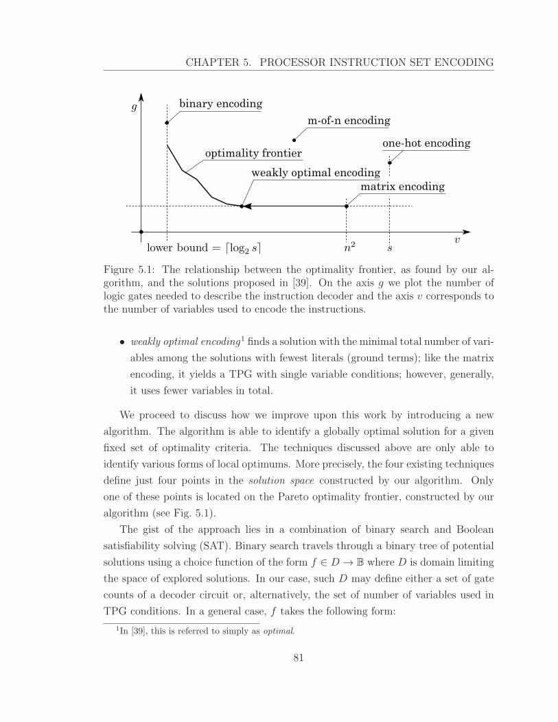
CHAPTER 5. PROCESSOR INSTRUCTION SET ENCODING
binary encoding
one-hot encoding
matrix encoding
weakly optimal encoding
m-of-n encoding
optimality frontier
Figure 5.1: The relationship between the optimality frontier, as found by our al-gorithm, and the solutions proposed in [39]. On the axis g we plot the number oflogic gates needed to describe the instruction decoder and the axis v corresponds tothe number of variables used to encode the instructions.
• weakly optimal encoding1 finds a solution with the minimal total number of vari-
ables among the solutions with fewest literals (ground terms); like the matrix
encoding, it yields a TPG with single variable conditions; however, generally,
it uses fewer variables in total.
We proceed to discuss how we improve upon this work by introducing a new
algorithm. The algorithm is able to identify a globally optimal solution for a given
fixed set of optimality criteria. The techniques discussed above are only able to
identify various forms of local optimums. More precisely, the four existing techniques
define just four points in the solution space constructed by our algorithm. Only
one of these points is located on the Pareto optimality frontier, constructed by our
algorithm (see Fig. 5.1).
The gist of the approach lies in a combination of binary search and Boolean
satisfiability solving (SAT). Binary search travels through a binary tree of potential
solutions using a choice function of the form f ∈ D → B where D is domain limiting
the space of explored solutions. In our case, such D may define either a set of gate
counts of a decoder circuit or, alternatively, the set of number of variables used in
TPG conditions. In a general case, f takes the following form:
1In [39], this is referred to simply as optimal.
81
CHAPTER 5. PROCESSOR INSTRUCTION SET ENCODING
f(x) =
{
1, when there exists a solution S such that its cost is x
0, otherwise
Such function f may be challenging to compute since the set from which solutions
are drawn is typically large. Let v and g signify the maximum number of variables
and gates; also let s be the number of scenarious encoded in the original TPG. Then
the size of the solutions space is in the order of
(2(v + g))2g (2v)s
For instance, for v = 5, g = 5 and s = 5 the formula above gives circa 1021 potential
solutions to consider. Clearly, computing f with a brute-force approach is infeasible.
Note, however, that f has a form of an existential quantifier binding indentifiers
to finite domains. This form of statement is perfectly suited for SAT solving. To
bridge to the SAT-level notation we have to do binary vector encoding of scenario
and variable indices, gate identifiers and cost indicators. The result is processed
by a SAT solver and the output is a binary representation of a decoding circuit. In
particular, we have used MiniSat [23] and clasp [12] SAT solvers. As one example,
we have been able to obtain an optimal solution for v = 8, s = 8 and g ∈ 3..12.
5.2 Problem statement
In microcontroller design, the encoding of an instruction set is a common reoccur-
ing problem. A form of encoding optimality is essential to achieve a more compact
instruction decoder logic, while, at the same time, offering higher decoding perform-
ance. The first step is to represent each instruction microcode as a TPG scenario.
Such scenario is a program each instruction of each is a reference to a microcon-
troller unit. The directed graph semantics underlaying PGs expresses the casual
dependendencies between events of unit firings; informally, this means that instruc-
tion execution steps may be ordered sequentially or concurrently.
An encoding scheme must ensure that every scenario is adeqautely represented
in the composed graph. This property, called the encoding correctness condition, is
formulated by the following statement
82
CHAPTER 5. PROCESSOR INSTRUCTION SET ENCODING
Si = G |X=θi
here X is the set of free variables of PG G (Chapter 4), Si is a scenario from a
scenario set S and X = θi stands for∧
x∈X x = θi(x). The condition states that
a scenario is properly decoded by applying an opcode-defined graph specialisation
θ. Every encoding schema may be characterised by a specific choice of set X and
encoding function θ. We refer to a tuple of (X, θ) as encoding of a scenario set S.
To uniquely determine, upto PG equivalence, and for encoding and scenario set
a compositional graph G one also needs to consider the property of composition
minimality :
G =∑
i<n
[X = θi](G |X=θi)
Informally, the condition states that G does not contain anything in addition to the
encoding of scenarios S.
To give an intuition behind encoding we shall consider a simple case of encoding
for two scnearios S1, S2. This encoding is constructed by putting together, in a
certain manner, graphs S1 and S2. More precisely, we overlay the graphs of S1 and
S2 using the + operator:
Gdf= [X = θ1]S1 + [X = θ2]S2
The overlaid graphs are conditioned by their opcodes. In the above, θ1, θ2 is a unique
value of vector X identifying a given scenario.
In a general case, for n scenarios, this statement takes the following form:
Gdf=∑
i<n
[X = θi]Si
Such encoding constructing preserves the property of composition mininimality provided
the correctness property also holds. Let us now briefly consider one particilar en-
coding scheme - the one hot encoding - to the composition of scenarios S1, S2:
Gdf= [x1 = 1 ∧ x2 = 0]S1 + [x1 = 0 ∧ x2 = 1]S2
83
CHAPTER 5. PROCESSOR INSTRUCTION SET ENCODING
It is easy to check that one hot encoding satisfies the correctness condition. For
instance, for the case of scenario S1, we can prove that the scenario can be obtained
via graph G specialisation as follows:
S1 = ([x1 = 1 ∧ x2 = 0]S1 + [x1 = 0 ∧ x2 = 1]S2) |x1=1∧x2=0
which is obviously correct by the definition of the specialisation operator H|p.
A common measure of complexity of a Boolean formula f is denoted as C(f) and
is defined to be the total count of literals in it, e.g. C(x · z + y · z) = 4, C(1) = 0,
etc. This is the metric used in [39] to assess the produced encodings. Indeed, when
applied to a single formula this metric often works well: the more literals the formula
has, the larger the circuit to evaluate this formula. However, when used to assess
multiple similar formulae or a single formula with repeating sub-formulae, this metric
fails to account for the fact that the outputs of logic gates evaluating the subformulae
can be reused. To take advantage of this fact we use the new metric G(C), showing
the total number of gates in the circuit needed to compute all of the conditions found
in C. We use two versions of this metric, differing in type of gates allowed: one with
AND/OR gates with all possible input and output inversions and another one with
NAND-gates only.
5.2.1 Overview
In this section we briefly discuss the encoding approaches developed in [39]. We
implement as SAT-based solution for the pre-existing techniques (weakly optimal
encoding) and introduce a new, more powerful technique for identifying globally
optimal solutions.
One hot
The one hot encoding scheme associates a unique indicator variable (a hot wire)
with each scenario. The set of free variables is exactly that of the scenarios being
encoded:
X = S
84
CHAPTER 5. PROCESSOR INSTRUCTION SET ENCODING
where S is the scenario set. The encoding is very simple: one sets i-th bit to 1 to
select an i-th scenario and the rest must be reset to zero:
θi(s) = (Si = s), where s, Si ∈ S
Matrix encoding
The matrix encoding allocates a unique variable for each edge and vertex of scenario
graphs Si. Hence, the set of free variables is given as
X = {0} × V ∪ {1} × E
An encoding bit is set depending on whether a given edge or vertex are included in
a given scenario s:
θi(0, v) = Ci(v), where v ∈ Vi
θi(1, e) = Di(e), where e ∈ Ei
where scenario Si is defined by a PG of the form (Vi, Ei, Ci, Di, Xi).
Binary encoding
Binary encoding associates a scenario index with the value of binary number coded
by an instruction opcode. One specific form of X can be given as
X = 1..⌈log |S|⌉
where S is the scenario set.
The encoding function computes the k-th bit of i-th scenario opcode as a binary
encoding of a natural number representing the scenario index:
θi(k) =
⌊
i− 1
2k−1
⌋
mod 2, where k is the bit position
Weakly optimal
The optimal encoding with unconstrained code length, which we call weakly optimal
encoding, tries to minimize the size of set X within the universe of solutions with
85
CHAPTER 5. PROCESSOR INSTRUCTION SET ENCODING
1-restricted conditions. We say that a graph is 1-restricted if all the edge and vertex
conditions contain at most one literal. It has been shown in [39] that the problem
of computing a weakly optimal encoding is NP-complete thus barring any attempts
at brute force solutions. It is challenging to give a compact characterisation of
optimal encoding in the terms of free variable set X and coding function θ. In
the continuation of the Chapter we shall give a SAT formulation of this encoding
approach.
5.2.2 Globally optimal encoding
The weakly optimal encoding method presented above generates the smallest PG
description of a set of partial orders but the number of used variables cannot be
controlled; in many practical cases it will use more variables than is affordable under
the design or technology constraints. In this section we briefly describe a method for
generating the smallest PG given a limit on the number of variables, i.e. given the
required length of the instruction codes.
Let L be the given limit on the number of variables. We generate all non-trivial
encoding constraints and try to satisfy them with opcode variables. Only L of them
are free variables X = {x1, x2, ..., xL}; other variables F = {f1, f2, ..., fm} are
not free — they are expressed in terms of variables from X ∪F using Boolean binary
functions, e.g. f1 = x1 + x3, f2 = f1 · x2, etc. As L is fixed all we have to do is to
minimise the number of non-free variables m. This minimisation problem requires
exploration of large search space; fortunately, it still belongs to the NP complexity
class and we can reduce it to the SAT problem: the solver has to ‘guess’ all the
opcodes, formulae of variables in F , and allocation of all variables X ∪ F to the
non-trivial encoding constraints.
5.3 SAT formulation
This section presents SAT formulations of the optimal encoding problems described
in the previous section.
The Boolean satisfiability problem (SAT) is to decide whether a given Boolean
formula F (x1, x2, . . . , xn) is satisfiable or not, i.e. if it is possible to find an assign-
86
CHAPTER 5. PROCESSOR INSTRUCTION SET ENCODING
ment of Boolean values (α1, α2, . . . , αn) ∈ {0, 1}n to the variables (x1, x2, . . . , xn)
which makes the formula true: F (α1, α2, . . . , αn) = 1. As SAT is a decision (not
optimisation) problem, we define a cost function and use a binary search to minimise
its value by calling the SAT solver with different cost constraints.
We have implemented all the techniques presented in this section in an automated
software tool which uses MiniSat [23] and clasp [12] as SAT solver engines. They
operate on CNF (conjunctive normal form) representations of Boolean formulae.
Since our SAT-instances are not necessarily given in CNF, we implemented their
automated conversion to CNF formulae. This conversion introduces intermediate
variables but the overall size of the obtained formula is linear with respect to the
size of the given SAT-instance.
5.3.1 Weakly optimal encoding
To solve the weakly optimal encoding problem described in Subsection 5.2 we min-
imise the number of colours used for a conflict graph colouring. Minimisation is
performed by solving a series of instances of the following decision problem.
Let G = (V, E) be an extended conflict graph, where vertices V correspond to
encoding constraints and edges E ⊆ V × V to conflicts between them. V contains
both original Vo = {e1, e2, . . . , en} and inverted Vi = {e1, e2, . . . , en} constraints,
such that V = Vo ∪ Vi. The problem is to find a colouring of G which uses no more
than m colours.
For every pair of vertices (ek, ek) we introduce a Boolean variable pk and an
integer number ck whose values have to be found by the SAT solver: pk indicates
which of the two vertices is coloured – if pk = 1 (resp. pk = 0) then ek (resp. ek) is
coloured, while ck represents the colour of the chosen vertex.
The SAT problem ENCODE consists of four constraints:
ENCODE = NUM · COLoo · COLoi · COLii
where NUM restricts colours such that 0 ≤ ck < m. Encoding of numbers ck in
Boolean domain can be different, for example, if we use binary encoding we need
⌈log2m⌉ bits for each ck. Implementation of NUM depends on the chosen encoding;
87
CHAPTER 5. PROCESSOR INSTRUCTION SET ENCODING
its general form is:
NUM =∏
1≤k≤n
(0 ≤ ck) · (ck < m)
Constraints COL check that adjacent vertices are assigned different colours:
COLoo =∏
(ej , ek)∈E∩(Vo×Vo)
(pj · pk) ⇒ (cj 6= ck)
COLoi =∏
(ej , ek)∈E∩(Vo×Vi)
(pj · pk) ⇒ (cj 6= ck)
COLii =∏
(ej , ek)∈E∩(Vi×Vi)
(pj · pk) ⇒ (cj 6= ck)
If we assume that complexity of comparison operations over numbers ck is C, then
the overall complexity of ENCODE is Θ((|V | + |E|) · C). In particular, in case of
binary encodings2 the complexity is Θ((|V |+ |E|) · logm). Depending on the chosen
number encodings, there are from Θ(|V | · logm) to Θ(|V | ·m) free variables.
If L is the minimum value of m for which formula ENCODE is satisfiable then
the optimal encoding uses L variables X = {x1, x2, ..., xL}. Values pk and ck which
satisfy the formula are used to resolve encoding constraints ek in the following way:
if pk = 1 then ek is resolved by xck , otherwise it is resolved by xck .
5.3.2 Globally optimal encoding
The version of the optimal encoding problem with constrained code length is signi-
ficantly more complicated and computationally intensive. It requires finding a set of
Boolean functions of L arguments (where L is the specified code length) and there
are 22L
of them – it is impossible to explore search spaces of such magnitudes, e.g.
228
roughly equals to the number of atoms in the universe. To cope with this, we
reduce the search space to 2-argument Boolean functions only. From the practical
point of view this is justified by the fact that most modern technology libraries con-
tain only 2- or 3-input logic gates anyway. Importantly, every complex function can
2Formula (a < b) for binary numbers comparison is (a < b) = a0 · b0 + (a0 = b0) · (a′ < b′)
where a′ and b′ are obtained from a and b by removal of their most significant digits (a0 and b0);the formula is linear with respect to the lengths of a and b.
88

CHAPTER 5. PROCESSOR INSTRUCTION SET ENCODING
be represented as a composition of simpler ones, therefore our approach can find
any function, albeit at the cost of introducing intermediate variables. This is similar
to what actually happens during technology mapping and logic decomposition of
functional components into hardware gates [14][19].
Formally, let (e1, e2, . . . , en) be a set of encoding constraints defined in Sub-
section 5.2, S be the number of scenarios, and L be the required code length. We
are looking for such a vector (ψ1, ψ2, . . . , ψS) of L-bit encodings and n functions
Fj, 1 ≤ j ≤ n such that Fj(ψk) = ej[k] for every scenario 1 ≤ k ≤ S (unless ej[k] is
a don’t care value).
We represent a set of functions F as a combinational circuit consisting of G 2-
input Boolean gates, where G is the value to be minimised. An output of the circuit
can be taken directly from one of its inputs or be produced by a gate. In addition,
any output can be inverted:
Fj(ψ) = select(Signals(ψ), oSelector j)⊕ Inv j
Here Signals(ψ) is a function computing all circuit signals including both circuit
inputs (given by parameter ψ) and gate outputs, oSelector j is the number indicating
which circuit signal is ‘connected’ to the j-th circuit output, function select(V , k)
selects k-th element from a given vector V , and Invj = 1 iff j-th circuit output
is inverted. Implementation of function select(V, k) depends on the encoding of k
(we used one-hot encoding in this case, which allows for simpler implementation).
Circuit signals are computed as follows:
Signals(ψ) = WiresG(ψ)
Wiresk(ψ) =
ψ if k = 0
Wiresk−1(ψ) ◦Gatek(ψ) if 0 < k ≤ G
Gatek(ψ) = arg1,k(ψ) · arg2,k(ψ)
arg j,k(ψ) = select(Wiresk−1(ψ), aSelector j,k)⊕ InvArg j,k
In other words, a set of wires is initially equal to the set of circuit inputs (Wires0(ψ) =
ψ) and then is iteratively extended by appending Gatek to the previously computed
set of wires Wiresk−1. Eventually, after G iterations we obtain the set of all signals
89
CHAPTER 5. PROCESSOR INSTRUCTION SET ENCODING
Signals(ψ) = WiresG(ψ). Every Gatek corresponds to an AND gate with possible
input inversions (indicated by InvArg0,k and InvArg1,k). Its arguments are selected by
aSelector 0,k and aSelector 1,k from the set of wires computed in the previous iteration.
This guarantees the absence of combinational loops.
As every signal in the circuit can be optionally inverted (by setting Inv j = 1 or
InvArg j,k = 1), the resultant gate basis includes 8 logic gates: AND, OR, NAND,
NOR, plus 4 other gates, obtained from these by inversion of exactly one of their
inputs (they do not have commonly adopted names, apart, perhaps, from Boolean
implication x ⇒ y which corresponds to OR(x, y)). We have also investigated a
simpler basis, consisting of only NAND gates with no optional input inversions. The
basis leads to smaller search space and works faster, but, as expected, produces larger
circuits (see Figure 5.6 for a comparison of two bases on a processor example). If the
NAND basis is used then free variables InvArg j,k can be dropped and the formulae
for Gatek(ψ) and arg j,k(ψ) should be modified as follows:
Gatek(ψ) = arg1,k(ψ) · arg2,k(ψ)
arg j,k(ψ) = select(Wiresk−1(ψ), aSelector j,k)
We tried to extend the 8-gate basis by addition of gates XOR and XNOR but on
practical examples it did not bring any benefit in terms of the number of used gates,
while significantly increasing the computation time (due to additional free variables
IsXork and more complex Gatek(ψ) functions).
In case of the standard 8-gate basis the SAT solver has to assign the following free
variables: ψj[k] (1 ≤ j ≤ S, 1 ≤ k ≤ L), Invj (1 ≤ j ≤ n), InvArg0,j and InvArg1,j
(1 ≤ j ≤ G). Also it has to find numbers oSelector j (1 ≤ j ≤ n), aSelector 0,j and
aSelector 1,j (1 ≤ j ≤ G). All other variables are derived.
The SAT problem ENCODE consists of two constraints:
ENCODE = NUM · EVAL
90
CHAPTER 5. PROCESSOR INSTRUCTION SET ENCODING
Constraint NUM restricts all the selectors to their domains:
NUM =∏
1≤j≤n
(1 ≤ oSelector j) · (oSelector j ≤ L+G)·
·∏
1≤j≤2
1≤k≤G
(1 ≤ aSelector j,k) · (aSelector j,k < L+ k) (5.1)
Constraint EVAL checks that the circuit outputs satisfy the encoding constraints:
∏
1≤j≤n1≤k≤S
(ej[k] 6= −) ⇒ (Fj(ψk) ⇔ ej[k])
If Gmin is the minimum value of G for which formula ENCODE is satisfiable then
the optimal encoding is obtained in vectors ψj (1 ≤ j ≤ S), an encoding constraint
ek is resolved by function Fj(ψ), and the circuit which produces these functions
contains Gmin gates.
We tried binary and one-hot number encodings in our implementation. In both
cases the complexity of the formula is Θ(S ·G ·(G+L)). The number of free variables
is Θ(S · L+ (G+ n) · C), where C is log(G+ L) and G+ L for binary and one-hot
encodings, respectively. In practice, one-hot encoding proved to be more efficient
despite significantly larger number of free variables. This can be explained by the
fact that one-hot encoding leads to simpler constraints.
5.3.3 Support for dynamic variables
A lot of practical applications require the use of dynamic variables, i.e. such variables
that can change their values during execution of a partial order and affect its further
execution flow [39]. An example of such application, a processor microcontroller, is
discussed in the next section.
Dynamic variables manifest themselves as encoding constraints with non-constant
elements, e.g. e = 110y1y, which means that in the fourth scenario the correspond-
ing condition has to evaluate to some dynamic variable y and in the sixth scenario it
has to evaluate to y. To compute the optimal encoding with such non-constant con-
straints we have to modify the method from the previous subsection in the following
way.
91
CHAPTER 5. PROCESSOR INSTRUCTION SET ENCODING
Let y be a dynamic variable. We generate formula ENCODE0 (resp. ENCODE1)
using encoding constraints where y is replaced by 0 (resp. 1). Note that the free
variables in both formulae have to be the same and we have to add y into the set
of circuit inputs. Then we use the SAT solver to find an assignment that satisfies
ENCODE0 · ENCODE1. Interpretation of the resulting assignment is the same
apart from the added input signal y. In case of more than one dynamic variable, the
process should be repeated for each of them. Potentially this leads to an exponential
explosion of the formula. Fortunately, the number of dynamic variables is rather
small in practice, thus the explosion is not dramatic.
It is still possible to avoid the explosion of the formula by conversion of the
problem into an instance of 2-QBF problem (a quantified Boolean formula with two
quantifiers [55]):
∃X ∀Y ENCODE
where X represents the set of all free variables, and Y stands for the set of dynamic
variables. However, conversion of a formula into 2-QBF does not necessarily reduce
the computation time needed to find its satisfying assignment. Implementation of a
tool based on a 2-QBF solver is a subject of future work.
The next section demonstrates application of this technique in a processor mi-
crocontroller design.
5.4 Processor design example
This section demonstrates application of TPG-algebra to designing processor micro-
controllers. Specification of such a complex system as a processor has to start at
the architectural level, which helps to manage the system complexity by structural
abstraction [19].
Fig. 5.2 shows the architecture of an example processor. Separate Program
memory and Data memory blocks are accessed via the Instruction fetch (IFU) and
Memory access (MAU) units, respectively. The other two operational units are:
Arithmetic logic unit (ALU) and Program counter increment unit (PCIU). The units
are controlled using request-acknowledgement interfaces (depicted as bidirectional
arrows) by the Central microcontroller, which is our primary design objective.
92
CHAPTER 5. PROCESSOR INSTRUCTION SET ENCODING
The processor has four registers: two general purpose registers A and B, Program
counter (PC) storing the address of the current instruction in the program memory,
and the Instruction register (IR) storing the opcode (operation code) of the current
instruction. For the purpose of this chapter, the actual width of the registers (the
number of bits they can store) is not important. ALU has access to all the registers
via the register bus; MAU has access to general purpose registers only; IFU, given
the address of the next instruction in PC, reads its opcode into IR; and PCIU is
responsible for incrementing PC (moving to the next instruction). The microcon-
troller has access to the IR and ALU flags (information about the current state of
ALU which is used in branching instructions).
Now we define the set of instructions of the processor. Rather than listing all the
instructions, we describe classes of instructions with the same addressing mode [1]
and the same execution scenario. As the scenarios here are partial orders of actions,
we use TPG-algebra, and the corresponding TPGs are shown in Fig. 5.3.
ALU operation Rn to Rn An instruction from this class takes two operands
stored in the general purpose registers (A and B), performs an operation, and writes
the result back into one of the registers (so called register direct addressing mode).
Examples: ADD A, B – addition A := A + B; MOV B , A – assignment B := A.
ALU works concurrently with PCIU and IFU, which is captured by the expression
ALU + PCIU → IFU ; the corresponding PG is shown in Fig. 5.3(a). As soon as
both concurrent branches are completed, the processor is ready to execute the next
instruction. Note that it is not important for the microcontroller which particular
ALU operation is being executed (ADD , MOV , or any other instruction from this
class) because the scenario is the same from its point of view (it is the responsibility
of ALU to detect which operation it has to perform according to the current opcode).
ALU operation #123 to Rn In this class of instructions one of the oper-
ands is a register and the other is a constant which is given immediately after the
instruction opcode (e.g. SUB A, #5 – subtraction A := A − 5), so called immedi-
ate addressing mode. At first, the constant has to be fetched into IR, modelled as
PCIU → IFU . Then ALU is executed concurrently with another increment of PC:
ALU + PCIU ′ (we use ′ to distinguish the different occurrences of actions of the
same unit). Finally, it is possible to fetch the next instruction into IR: IFU ′. The
overall scenario is then PCIU → IFU → (ALU + PCIU ′) → IFU ′.
93
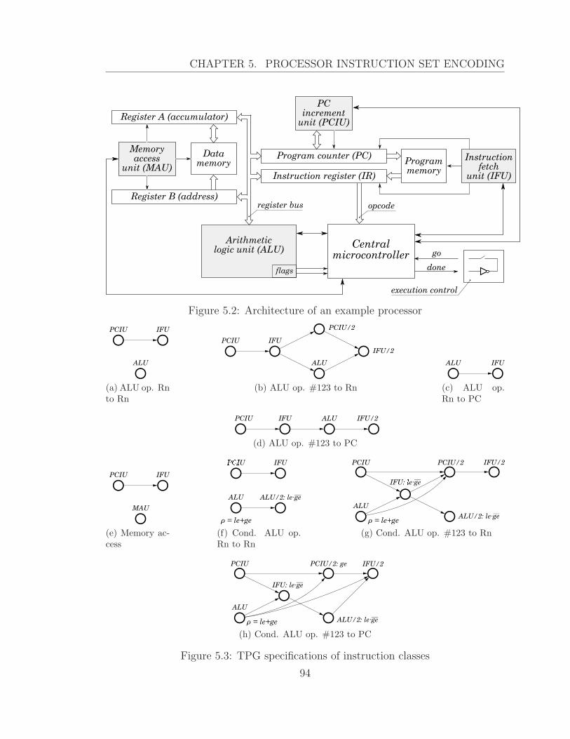
CHAPTER 5. PROCESSOR INSTRUCTION SET ENCODING
Program counter (PC)
Instruction register (IR)
Programmemory
Register A (accumulator)
Register B (address)
Instructionfetch
unit (IFU)
Centralmicrocontroller
opcode
PCincrement
unit (PCIU)
Memoryaccess
unit (MAU)
Datamemory
register bus
go
done
execution control
Arithmeticlogic unit (ALU)
flags
Figure 5.2: Architecture of an example processor
ALU
PCIU IFU
(a) ALU op. Rnto Rn
PCIU
ALU
IFU
PCIU/2
IFU/2
(b) ALU op. #123 to Rn
ALU IFU
(c) ALU op.Rn to PC
PCIU IFU/2IFU ALU
(d) ALU op. #123 to PC
MAU
PCIU IFU
(e) Memory ac-cess
ALU
IFU���U
ρ = le+ge
ALU/2: le∙ge_
(f) Cond. ALU op.Rn to Rn
ALU
IFU: �e∙ge
IFU/2PCIU/2PCIU
ρ = le+geALU/2: le∙ge
_
_
(g) Cond. ALU op. #123 to Rn
IFU: le∙ge
IFU/2PCIU
ALU
ALU/2: le∙ge
PCIU/2: ge
ρ = le+ge
_
_
(h) Cond. ALU op. #123 to PC
Figure 5.3: TPG specifications of instruction classes
94
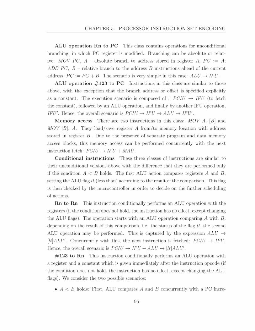
CHAPTER 5. PROCESSOR INSTRUCTION SET ENCODING
ALU operation Rn to PC This class contains operations for unconditional
branching, in which PC register is modified. Branching can be absolute or relat-
ive: MOV PC , A – absolute branch to address stored in register A, PC := A;
ADD PC , B – relative branch to the address B instructions ahead of the current
address, PC := PC + B. The scenario is very simple in this case: ALU → IFU .
ALU operation #123 to PC Instructions in this class are similar to those
above, with the exception that the branch address or offset is specified explicitly
as a constant. The execution scenario is composed of : PCIU → IFU (to fetch
the constant), followed by an ALU operation, and finally by another IFU operation,
IFU ′. Hence, the overall scenario is PCIU → IFU → ALU → IFU ′.
Memory access There are two instructions in this class: MOV A, [B ] and
MOV [B ], A. They load/save register A from/to memory location with address
stored in register B. Due to the presence of separate program and data memory
access blocks, this memory access can be performed concurrently with the next
instruction fetch: PCIU → IFU +MAU .
Conditional instructions These three classes of instructions are similar to
their unconditional versions above with the difference that they are performed only
if the condition A < B holds. The first ALU action compares registers A and B,
setting the ALU flag lt (less than) according to the result of the comparison. This flag
is then checked by the microcontroller in order to decide on the further scheduling
of actions.
Rn to Rn This instruction conditionally performs an ALU operation with the
registers (if the condition does not hold, the instruction has no effect, except changing
the ALU flags). The operation starts with an ALU operation comparing A with B;
depending on the result of this comparison, i.e. the status of the flag lt, the second
ALU operation may be performed. This is captured by the expression ALU →
[lt]ALU ′. Concurrently with this, the next instruction is fetched: PCIU → IFU .
Hence, the overall scenario is PCIU → IFU + ALU → [lt]ALU ′.
#123 to Rn This instruction conditionally performs an ALU operation with
a register and a constant which is given immediately after the instruction opcode (if
the condition does not hold, the instruction has no effect, except changing the ALU
flags). We consider the two possible scenarios:
• A < B holds: First, ALU compares A and B concurrently with a PC incre-
95
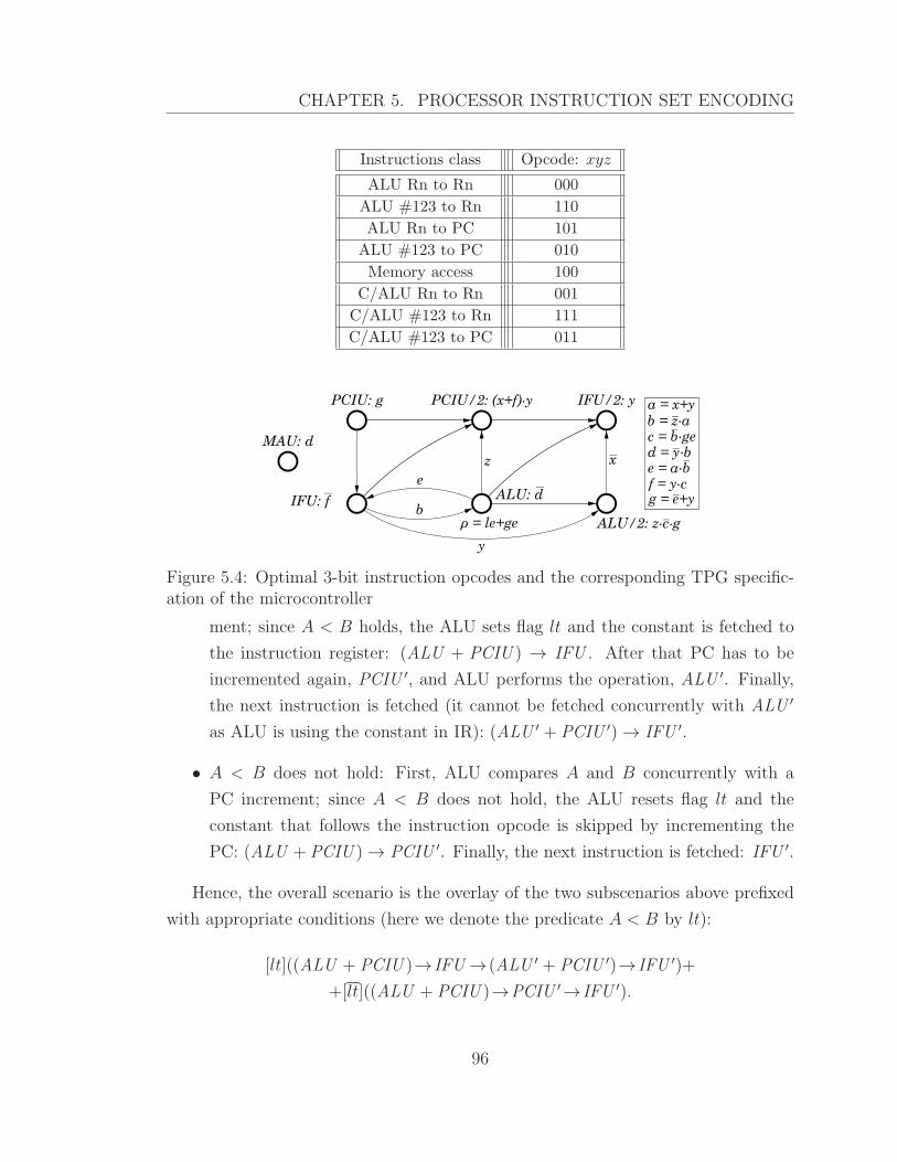
CHAPTER 5. PROCESSOR INSTRUCTION SET ENCODING
Instructions class Opcode: xyz
ALU Rn to Rn 000
ALU #123 to Rn 110
ALU Rn to PC 101
ALU #123 to PC 010
Memory access 100
C/ALU Rn to Rn 001
C/ALU #123 to Rn 111
C/ALU #123 to PC 011
MAU: d
PCIU: g
b
e
PCIU/2: (x+f) y
ALU: d
IFU/2: y
x
ALU/2: z c g_
ρ = le+ge
IFU: f_
y
_
_
z
. .
a = x+y
g = e+y_
b = z a_.
c = b ge_.
d = y b_.
e = a b_
.
f = y c.
.
Figure 5.4: Optimal 3-bit instruction opcodes and the corresponding TPG specific-ation of the microcontroller
ment; since A < B holds, the ALU sets flag lt and the constant is fetched to
the instruction register: (ALU + PCIU ) → IFU . After that PC has to be
incremented again, PCIU ′, and ALU performs the operation, ALU ′. Finally,
the next instruction is fetched (it cannot be fetched concurrently with ALU ′
as ALU is using the constant in IR): (ALU ′ + PCIU ′) → IFU ′.
• A < B does not hold: First, ALU compares A and B concurrently with a
PC increment; since A < B does not hold, the ALU resets flag lt and the
constant that follows the instruction opcode is skipped by incrementing the
PC: (ALU + PCIU ) → PCIU ′. Finally, the next instruction is fetched: IFU ′.
Hence, the overall scenario is the overlay of the two subscenarios above prefixed
with appropriate conditions (here we denote the predicate A < B by lt):
[lt]((ALU + PCIU )→IFU →(ALU ′ + PCIU ′)→IFU ′)+
+[lt]((ALU + PCIU )→PCIU ′→IFU ′).
96

CHAPTER 5. PROCESSOR INSTRUCTION SET ENCODING
This expression can be simplified using the rules of TPG-algebra:3
(ALU + PCIU )→ [lt]IFU →(PCIU ′ + [lt]ALU ′)→IFU ′.
#123 to PC This instruction performs a conditional branching in which the
branch address or offset is specified explicitly as a constant. We consider the two
possible scenarios:
• A < B holds: First, ALU compares A and B concurrently with a PC increment;
since A < B holds, the ALU sets flag lt and the constant is fetched to the
instruction register: (ALU + PCIU ) → IFU . After that ALU performs the
branching operation by modifying PC, ALU ′. After PC is changed, the next
instruction is fetched, IFU ′.
• A < B does not hold: the scenario is exactly the same as in the #123 to Rn
case when A < B does not hold.
Hence, the overall scenario is the overlay of the two subscenarios above prefixed with
appropriate conditions (here we denote the predicate A < B by lt):
[lt]((ALU + PCIU )→IFU →ALU ′→IFU ′)+
+[lt]((ALU + PCIU )→PCIU ′→IFU ′).
This expression can be simplified using the rules of TPG-algebra:
(ALU + PCIU )→([lt]PCIU ′ + [lt](IFU →ALU ′))→IFU ′.
The overall specification of the microcontroller can now be obtained by prefixing
the scenarios with appropriate conditions and overlaying them. These conditions
can be naturally derived from the instruction opcodes. The opcodes can be either
imposed externally or chosen with the view to optimise the microcontroller. In the
3This case illustrates the advantage of using the new hierarchical approach that allows to specifythe system as a composition of scenarios and formally manipulate them in an algebraic fashion.In our previous work [40], the CPOG for this class of instruction was designed monolithically, andbecause of this the arc between ALU ′ and IFU ′ was missed. Adding this arc not only fixes thedangerous race between these two blocks, but also leads to a smaller microcontroller due to theadditional similarity between TPGs for this class of instructions and for the one described below.
97
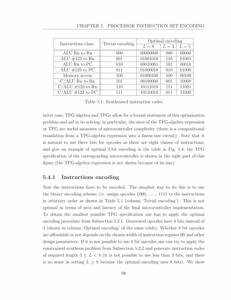
CHAPTER 5. PROCESSOR INSTRUCTION SET ENCODING
Instructions class Trivial encodingOptimal encoding
L = 8 L = 3 L = 5
ALU Rn to Rn 000 00000000 000 00000ALU #123 to Rn 001 01001010 110 01001ALU Rn to PC 010 00010001 101 00010
ALU #123 to PC 011 01000010 010 01000Memory access 100 01000100 100 00100
C/ALU Rn to Rn 101 00100000 001 10000C/ALU #123 to Rn 110 10111010 111 11001C/ALU #123 to PC 111 10110010 011 11000
Table 5.1: Synthesised instruction codes
latter case, TPG-algebra and TPGs allow for a formal statement of this optimisation
problem and aid in its solving; in particular, the sizes of the TPG-algebra expression
or TPG are useful measures of microcontroller complexity (there is a compositional
translation from a TPG-algebra expression into a linear-size circuit). Note that it
is natural to use three bits for opcodes as there are eight classes of instructions,
and give an example of optimal 3-bit encoding in the table in Fig. 5.4; the TPG
specification of the corresponding microcontroller is shown in the right part of this
figure (the TPG-algebra expression is not shown because of its size).
5.4.1 Instructions encoding
Now the instructions have to be encoded. The simplest way to do this is to use
the binary encoding scheme, i.e. assign opcodes {000, . . . , 111} to the instructions
in arbitrary order as shown in Table 5.1 (column ‘Trivial encoding’). This is not
optimal in terms of area and latency of the final microcontroller implementation.
To obtain the smallest possible TPG specification one has to apply the optimal
encoding procedure from Subsection 5.2.1. Generated opcodes have 8 bits instead of
3 (shown in column ‘Optimal encoding’ of the same table). Whether 8 bit opcodes
are affordable or not depends on the chosen width of instruction register IR and other
design parameters. If it is not possible to use 8 bit opcodes one can try to apply the
constrained synthesis problem from Subsection 5.2.2 and generate instruction codes
of required length 3 ≤ L < 8 (it is not possible to use less than 3 bits, and there
is no sense in setting L ≥ 8 because the optimal encoding uses 8 bits). We show
98
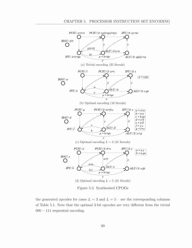
CHAPTER 5. PROCESSOR INSTRUCTION SET ENCODING
_MAU: xyz
_
PCIU: x+y+z_
IFU: x+y+ge_ _ _ xz
_
y(x+z)_
PCIU/2: xy(z+ge)+xyz_ __
y
ALU: x+y+z_
y
IFU/2: xy+xz_
z
ALU/2: xge(y+z)_
ρ = le+ge
(a) Trivial encoding (35 literals)
MAU: w
PCIU: t
y
u
PCIU/2: a+v
y
ALU: w
s
IFU/2: s
v
ALU/2: z ge_
a = x ge
ρ = le+ge
IFU: a_
__
_
_
.
.
(b) Optimal encoding (16 literals)
MAU: d
PCIU: g
b
e
PCIU/2: (x+f) y
ALU: d
IFU/2: y
x
ALU/2: z c g_
ρ = le+ge
IFU: f_
y
_
_
z
. .
a = x+y
g = e+y_
b = z a_.
c = b ge_.
d = y b_.
e = a b_
.
f = y c.
.
(c) Optimal encoding L = 3 (31 literals)
MAU: z
PCIU: u
a y
a+u
PCIU/2: b+v
a+y
ALU: z
y
IFU/2: y
v
ALU/2: x ge_
a = x yb = a ge
ρ = le+ge
IFU: b_
__
_
_
_
.
..
.
(d) Optimal encoding L = 5 (21 literals)
Figure 5.5: Synthesised CPOGs
the generated opcodes for cases L = 3 and L = 5 – see the corresponding columns
of Table 5.1. Note that the optimal 3-bit opcodes are very different from the trivial
000− 111 sequential encoding.
99
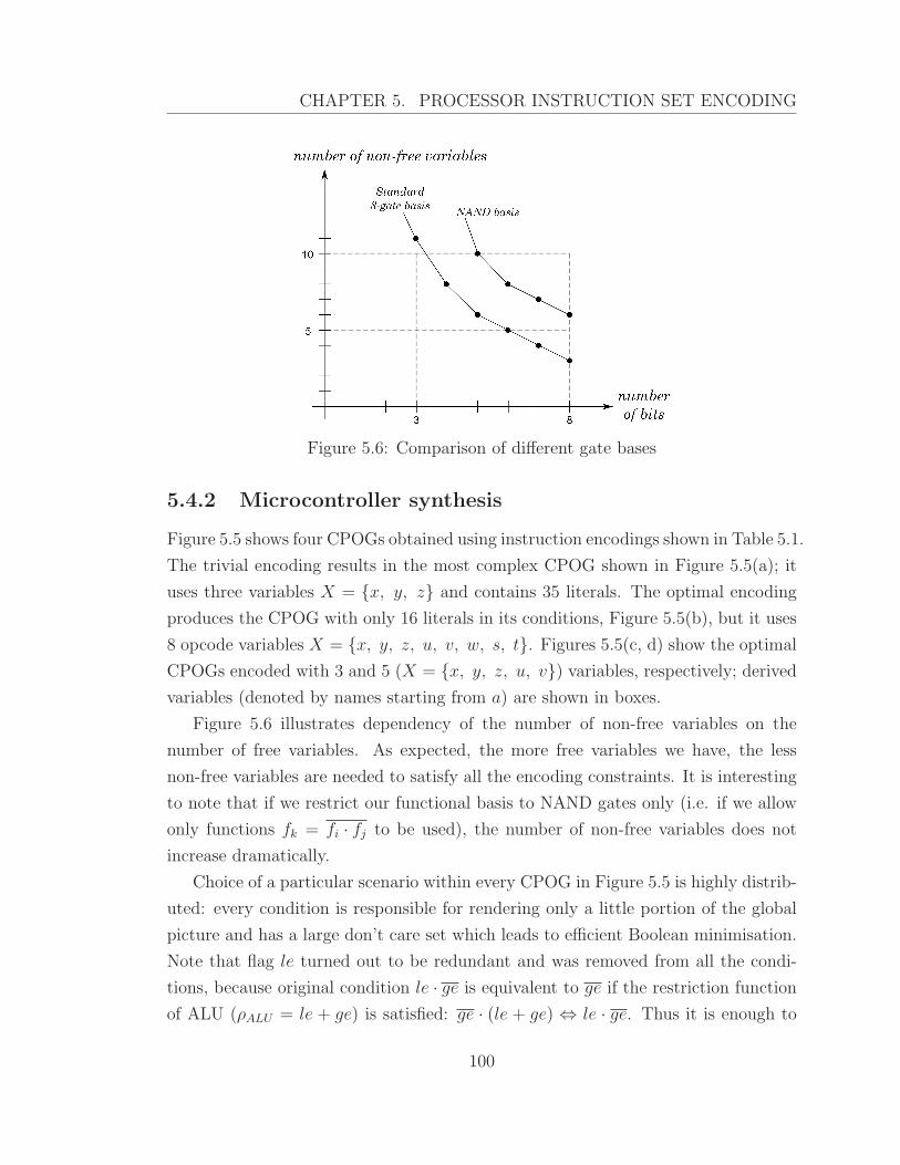
CHAPTER 5. PROCESSOR INSTRUCTION SET ENCODING
3 8
5
10
Figure 5.6: Comparison of different gate bases
5.4.2 Microcontroller synthesis
Figure 5.5 shows four CPOGs obtained using instruction encodings shown in Table 5.1.
The trivial encoding results in the most complex CPOG shown in Figure 5.5(a); it
uses three variables X = {x, y, z} and contains 35 literals. The optimal encoding
produces the CPOG with only 16 literals in its conditions, Figure 5.5(b), but it uses
8 opcode variables X = {x, y, z, u, v, w, s, t}. Figures 5.5(c, d) show the optimal
CPOGs encoded with 3 and 5 (X = {x, y, z, u, v}) variables, respectively; derived
variables (denoted by names starting from a) are shown in boxes.
Figure 5.6 illustrates dependency of the number of non-free variables on the
number of free variables. As expected, the more free variables we have, the less
non-free variables are needed to satisfy all the encoding constraints. It is interesting
to note that if we restrict our functional basis to NAND gates only (i.e. if we allow
only functions fk = fi · fj to be used), the number of non-free variables does not
increase dramatically.
Choice of a particular scenario within every CPOG in Figure 5.5 is highly distrib-
uted: every condition is responsible for rendering only a little portion of the global
picture and has a large don’t care set which leads to efficient Boolean minimisation.
Note that flag le turned out to be redundant and was removed from all the condi-
tions, because original condition le · ge is equivalent to ge if the restriction function
of ALU (ρALU = le + ge) is satisfied: ge · (le + ge) ⇔ le · ge. Thus it is enough to
100
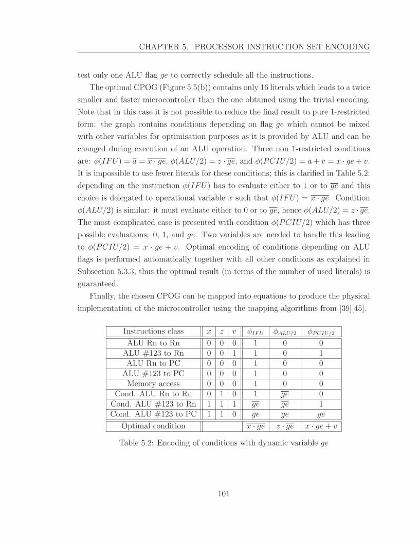
CHAPTER 5. PROCESSOR INSTRUCTION SET ENCODING
test only one ALU flag ge to correctly schedule all the instructions.
The optimal CPOG (Figure 5.5(b)) contains only 16 literals which leads to a twice
smaller and faster microcontroller than the one obtained using the trivial encoding.
Note that in this case it is not possible to reduce the final result to pure 1-restricted
form: the graph contains conditions depending on flag ge which cannot be mixed
with other variables for optimisation purposes as it is provided by ALU and can be
changed during execution of an ALU operation. Three non 1-restricted conditions
are: φ(IFU) = a = x · ge, φ(ALU/2) = z · ge, and φ(PCIU/2) = a+ v = x · ge+ v.
It is impossible to use fewer literals for these conditions; this is clarified in Table 5.2:
depending on the instruction φ(IFU) has to evaluate either to 1 or to ge and this
choice is delegated to operational variable x such that φ(IFU) = x · ge. Condition
φ(ALU/2) is similar: it must evaluate either to 0 or to ge, hence φ(ALU/2) = z · ge.
The most complicated case is presented with condition φ(PCIU/2) which has three
possible evaluations: 0, 1, and ge. Two variables are needed to handle this leading
to φ(PCIU/2) = x · ge + v. Optimal encoding of conditions depending on ALU
flags is performed automatically together with all other conditions as explained in
Subsection 5.3.3, thus the optimal result (in terms of the number of used literals) is
guaranteed.
Finally, the chosen CPOG can be mapped into equations to produce the physical
implementation of the microcontroller using the mapping algorithms from [39][45].
Instructions class x z v φIFU φALU/2 φPCIU/2
ALU Rn to Rn 0 0 0 1 0 0ALU #123 to Rn 0 0 1 1 0 1ALU Rn to PC 0 0 0 1 0 0
ALU #123 to PC 0 0 0 1 0 0Memory access 0 0 0 1 0 0
Cond. ALU Rn to Rn 0 1 0 1 ge 0Cond. ALU #123 to Rn 1 1 1 ge ge 1Cond. ALU #123 to PC 1 1 0 ge ge ge
Optimal condition x · ge z · ge x · ge+ v
Table 5.2: Encoding of conditions with dynamic variable ge
101
CHAPTER 5. PROCESSOR INSTRUCTION SET ENCODING
5.5 Summary
In this Chapter we have considered the problem of microcontroller instruction design
and encoding. We have shown how the application of Parametrised Graphs helps to
semi- or completely automatically derive the specification of entire controller from the
specification of individual instruction microcode. Crucially, the result is amenable
to further transformations possibly with automated rewriting tools.
We have developed a new technique for Parametrised Graph encoding that per-
mits the computation of the globally optimal solution to the PG encoding problem.
We do translation into a SAT instance to harness the power of SAT solving tools.
The proposal has important practical applications in microelectronics industry and
we plan to further pursue the fruitul direction.
102
Chapter 6
Conclusions
In this thesis we have presented a number of solutions to the problem of composi-
tional design of large scale digital circuits. These solutions help to synthesise efficient
asynchronous control circuits, transform and analyse compositional structures suit-
able for subsequent generation of hardware control logic and compute an efficient
encoding of micro-controller instruction set.
6.1 Improved parallel composition
In Chapter 3 we discussed an improved algorithm for computing the parallel compos-
ition of STGs or labelled Petri nets. The algorithm makes use of the FCI assumption
to produce nets with fewer implicit places. This aids in the synthesis of subsequent
structural algorithms like dummy contraction. It uses only simple structural checks
and thus is very efficient even for large compositions, so the improvement comes at
negligible cost.
The algorithm was implemented in the PComp tool and evaluated on a set of
scalable benchmarks. The experiments proved its efficiency, which increases even
more when the components are pre-processed to remove dummies and ensure in-
jective labelling (this is usually cheap, as the components are small; moreover, if
the components come from a standard library of component types, this step can be
completely eliminated).
Another important advantage is that the improved algorithm places almost no
additional effort on the user: the only requirement is to pass an additional command-
103
CHAPTER 6. CONCLUSIONS
line option to PComp so that it can assume the FCI property and apply the proposed
optimisation.
6.2 Parametrised Graphs theory
We introduced a new formalism called Parametrised Graphs and the corresponding
algebra. The formalism allows to manage a large number of system configurations
and execution modes, exploit similarities between them to simplify the specification,
and to work with groups of configurations and modes rather than with individual
ones. The modes and groups of modes can be managed in a compositional way, and
the specifications can be manipulated (transformed and/or optimised) algebraically
in a fully formal and natural way.
We develop two variants of the algebra of parametrised graphs, corresponding to
the two natural graph equivalences: graph isomorphism and isomorphism of trans-
itive closures. Both cases are specified axiomatically, and the soundness, minimality
and completeness of the resulting sets of axioms are formally proved. Moreover, the
canonical forms of algebraic terms are developed in each case.
We have formalised the definitions of algebra of parametrised graph in Agda, and
developed the machine-checked proofs of several properties of that algebra.
The formula representation data structure was designed together with the custom
structural equivalence relation on formula representations for convenient formula ma-
nipulations. The equivalence relation has been proved equivalent to the one defined
using formula semantics, thus showing its adequacy.
The normal form representation data structure for PG formulae was designed
with its semantics defined as translation to the corresponding general formula rep-
resentations. The algorithm of finding the normal form of general formulae was
developed and was proved to be correct.
The usefulness of the developed formalism has been demonstrated on two case
studies, a phase encoding controller and a processor micro-controller. Both have a
large number of execution scenarios, and the developed formalism allows to capture
them algebraically, by composing individual scenarios and groups of scenarios. The
possibility of algebraical manipulation was essential to obtain the optimised final
specification in each case.
104

CHAPTER 6. CONCLUSIONS
The developed formalism is also convenient for implementation in a tool, as ma-
nipulating algebraic terms is much easier than general graph manipulation; in par-
ticular, the theory of term rewriting can be naturally applied to derive the canonical
forms.
6.3 Processor instruction set encoding
The Chapter 5 presented the PG model based methodology for micro architecture
design and studied its application for specification and synthesis of a central pro-
cessor micro-controller. The key contribution is the method for synthesis of optimal
instruction op-codes; the corresponding optimisation problem is formulated in terms
of PGs and reduced to the well-known Boolean satisfiability problem. The method
is implemented in a software tool and can be used within the conventional micro
architecture design flow.
The studied processor example is purely academic. Nonetheless, it captures many
important features of real processors. It has been demonstrated that the PG model
is capable of modelling concurrency between different subsystems and handling mul-
tiple choice during instruction execution. Future work focuses on specification and
synthesis of a real processor and optimisation of the encoding algorithms.
Both have a large number of execution scenarios, and the developed formalism
allows to capture them algebraically, by composing individual scenarios and groups
of scenarios. The possibility of algebraical manipulation was essential to obtain the
optimised final specification in each case.
The developed formalism is also convenient for implementation in a tool, as ma-
nipulating algebraic terms is much easier than general graph manipulation; in par-
ticular, the theory of term rewriting can be naturally applied to derive the canonical
forms.
6.4 Future work
The improved parallel composition from Chapter 3 can be generalised by weakening
the test used in implicit place elimination and thus taking into the consideration
the non-trivial relationships between inputs and outputs. At the moment, we only
105
CHAPTER 6. CONCLUSIONS
remove placed directly connected to input and output transitions; a stronger version
of Proposition 1 would reason not at the level of individual places, immediately
connected to input/output transitions, but rather whole paths going from an output
transition to an input transition.
For Parametrised Graphs, we plan to automate the algebraic manipulation of
PGs, and implement automatic synthesis of PGs into digital circuits. For the latter,
much of the code developed for the precursor formalism of Conditional Partial Order
Graphs (CPOGs) can be re-used. One of the important problems that needs to be
automated is that of simplification of (T)PG expressions, in the sense of deriving an
equivalent expression with the minimum possible number of operators. Our prelimin-
ary research suggests that this problem is strongly related to modular decomposition
of graphs [37].
We also plan to formalise the proof of CPOG being a model of PG Algebra and
modification of the normalisation algorithm from Chapter 4 computing the canonical
form (where each graph node is mentioned no more than once) instead of just a
normal form. Canonical form is much more useful because its size is at most quadratic
while the size of a normal form is exponential in general. The canonical form is also
a way to quickly compare graphs and solve equational relations.
106
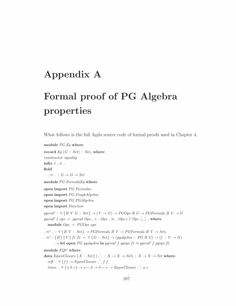
Appendix A
Formal proof of PG Algebra
properties
What follows is the full Agda source code of formal proofs used in Chapter 4.
module PG .Eq where
record Eq (G : Set) : Set1 where
constructor equality
infix 3 ≈
field
≈ : G → G → Set
module PG .FormulaEq where
open import PG .Formulae
open import PG .GraphAlgebra
open import PG .PGAlgebra
open import Function
pgeval ′ : ∀ {B V G : Set } → (V → G) → PGOps B G → PGFormula B V → G
pgeval ′ f ops = pgeval Ops . + Ops . ≫ Ops .ε f Ops . [ ] where
module Ops = PGOps ops
≈s : ∀ {B V : Set } → PGFormula B V → PGFormula B V → Set1
≈s {B } {V } f1 f2 = ∀ {G : Set } → (pgalgebra : PG B G) → (f : V → G)
→ let open PG pgalgebra in pgeval ′ f pgops f1 ≈ pgeval ′ f pgops f2
module EQC where
data EquivClosure {X : Set } ( ˜ : X → X → Set) : X → X → Set where
refl : ∀ {f } → EquivClosure ˜ f f
trans : ∀ {a b c} → a ∼ b → b ∼ c → EquivClosure ˜ a c
107
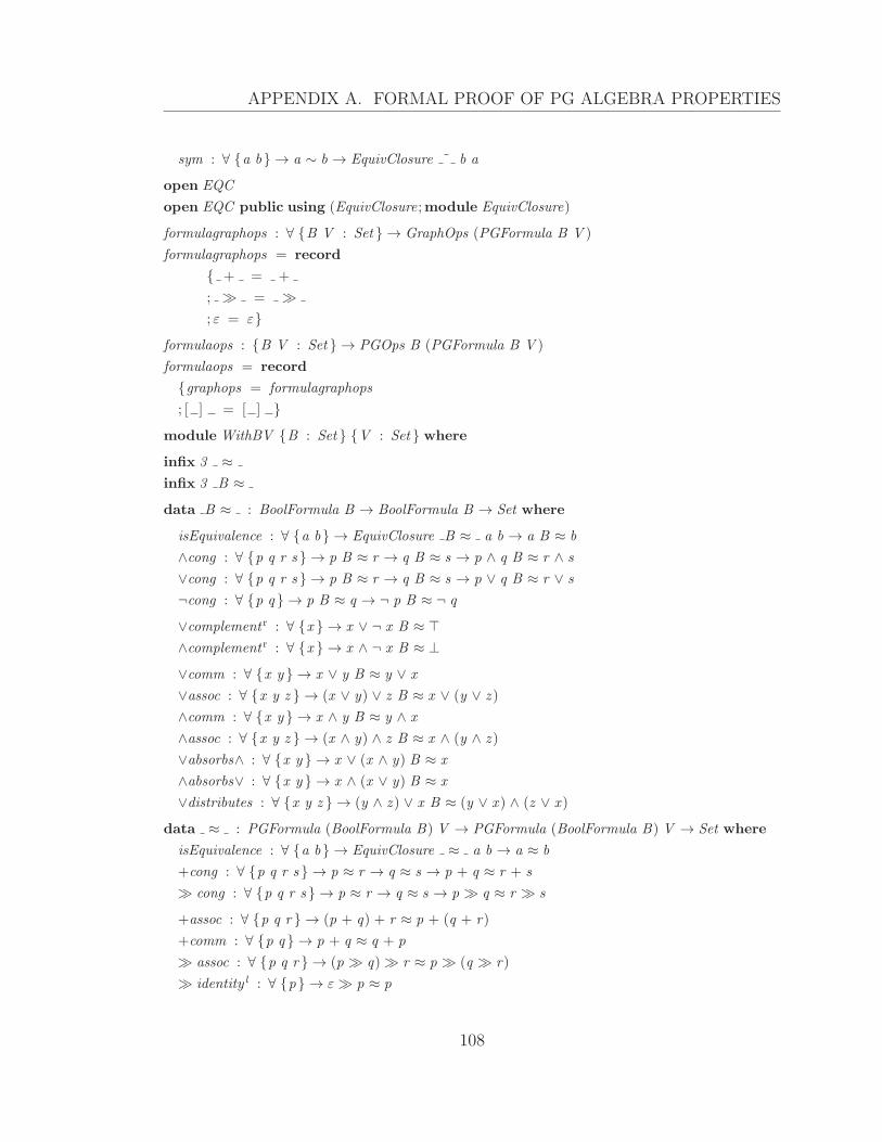
APPENDIX A. FORMAL PROOF OF PG ALGEBRA PROPERTIES
sym : ∀ {a b} → a ∼ b → EquivClosure ˜ b a
open EQC
open EQC public using (EquivClosure;module EquivClosure)
formulagraphops : ∀ {B V : Set } → GraphOps (PGFormula B V )
formulagraphops = record
{ + = +
; ≫ = ≫
; ε = ε}
formulaops : {B V : Set } → PGOps B (PGFormula B V )
formulaops = record
{graphops = formulagraphops
; [ ] = [ ] }
module WithBV {B : Set } {V : Set } where
infix 3 ≈
infix 3 B ≈
data B ≈ : BoolFormula B → BoolFormula B → Set where
isEquivalence : ∀ {a b} → EquivClosure B ≈ a b → a B ≈ b
∧cong : ∀ {p q r s } → p B ≈ r → q B ≈ s → p ∧ q B ≈ r ∧ s
∨cong : ∀ {p q r s } → p B ≈ r → q B ≈ s → p ∨ q B ≈ r ∨ s
¬cong : ∀ {p q } → p B ≈ q → ¬ p B ≈ ¬ q
∨complement r : ∀ {x } → x ∨ ¬ x B ≈ ⊤
∧complement r : ∀ {x } → x ∧ ¬ x B ≈ ⊥
∨comm : ∀ {x y } → x ∨ y B ≈ y ∨ x
∨assoc : ∀ {x y z } → (x ∨ y) ∨ z B ≈ x ∨ (y ∨ z )
∧comm : ∀ {x y } → x ∧ y B ≈ y ∧ x
∧assoc : ∀ {x y z } → (x ∧ y) ∧ z B ≈ x ∧ (y ∧ z )
∨absorbs∧ : ∀ {x y } → x ∨ (x ∧ y) B ≈ x
∧absorbs∨ : ∀ {x y } → x ∧ (x ∨ y) B ≈ x
∨distributes : ∀ {x y z } → (y ∧ z ) ∨ x B ≈ (y ∨ x ) ∧ (z ∨ x )
data ≈ : PGFormula (BoolFormula B) V → PGFormula (BoolFormula B) V → Set where
isEquivalence : ∀ {a b} → EquivClosure ≈ a b → a ≈ b
+cong : ∀ {p q r s } → p ≈ r → q ≈ s → p + q ≈ r + s
≫ cong : ∀ {p q r s } → p ≈ r → q ≈ s → p ≫ q ≈ r ≫ s
+assoc : ∀ {p q r } → (p + q) + r ≈ p + (q + r)
+comm : ∀ {p q } → p + q ≈ q + p
≫ assoc : ∀ {p q r } → (p ≫ q) ≫ r ≈ p ≫ (q ≫ r)
≫ identity l : ∀ {p} → ε ≫ p ≈ p
108
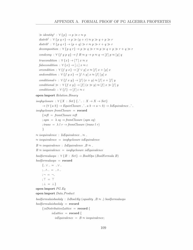
APPENDIX A. FORMAL PROOF OF PG ALGEBRA PROPERTIES
≫ identityr : ∀ {p} → p ≫ ε ≈ p
distribl : ∀ {p q r } → p ≫ (q + r) ≈ p ≫ q + p ≫ r
distribr : ∀ {p q r } → (p + q) ≫ r ≈ p ≫ r + q ≫ r
decomposition : ∀ {p q r } → p ≫ q ≫ r ≈ p ≫ q + p ≫ r + q ≫ r
condcong : ∀ {f g p q } → f B ≈ g → p ≈ q → [f ] p ≈ [g ] q
truecondition : ∀ {x } → [⊤ ] x ≈ x
falsecondition : ∀ {x } → [⊥ ] x ≈ ε
orcondition : ∀ {f g x } → [f ∨ g ] x ≈ [f ] x + [g ] x
andcondition : ∀ {f g x } → [f ∧ g ] x ≈ [f ] [g ] x
conditional+ : ∀ {f x y } → [f ] (x + y) ≈ [f ] x + [f ] y
conditional ≫ : ∀ {f x y } → [f ] (x ≫ y) ≈ [f ] x ≫ [f ] y
conditionalε : ∀ {f } → [f ] ε ≈ ε
open import Relation.Binary
iseqbyclosure : ∀ {X : Set } { ˜ : X → X → Set }
→ (∀ {a b} → EquivClosure ˜ a b → a ∼ b) → IsEquivalence ˜
iseqbyclosure fromClosure = record
{refl = fromClosure refl
; sym = λ eq → fromClosure (sym eq)
; trans = λ l r → fromClosure (trans l r)
}
≈ isequivalence : IsEquivalence ≈
≈ isequivalence = iseqbyclosure isEquivalence
B ≈ isequivalence : IsEquivalence B ≈
B ≈ isequivalence = iseqbyclosure isEquivalence
boolformulaops : ∀ {B : Set } → BoolOps (BoolFormula B)
boolformulaops = record
{ ∨ = ∨
; ∧ = ∧
;¬ = ¬
;⊤ = ⊤
;⊥ = ⊥}
open import PG .Eq
open import Data.Product
boolformulaisboolalg : IsBoolAlg (equality B ≈ ) boolformulaops
boolformulaisboolalg = record
{isDistributiveLattice = record {
isLattice = record {
isEquivalence = B ≈ isequivalence;
109
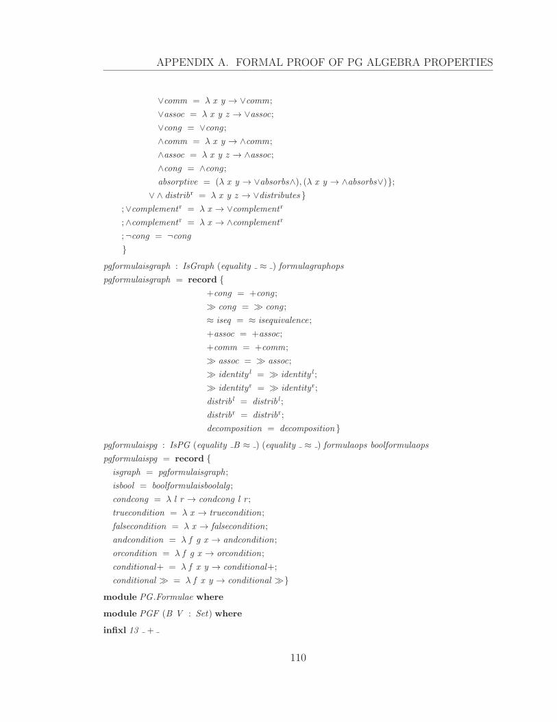
APPENDIX A. FORMAL PROOF OF PG ALGEBRA PROPERTIES
∨comm = λ x y → ∨comm;
∨assoc = λ x y z → ∨assoc;
∨cong = ∨cong ;
∧comm = λ x y → ∧comm;
∧assoc = λ x y z → ∧assoc;
∧cong = ∧cong ;
absorptive = (λ x y → ∨absorbs∧), (λ x y → ∧absorbs∨)};
∨ ∧ distribr = λ x y z → ∨distributes }
;∨complement r = λ x → ∨complement r
;∧complement r = λ x → ∧complement r
;¬cong = ¬cong
}
pgformulaisgraph : IsGraph (equality ≈ ) formulagraphops
pgformulaisgraph = record {
+cong = +cong ;
≫ cong = ≫ cong ;
≈ iseq = ≈ isequivalence;
+assoc = +assoc;
+comm = +comm;
≫ assoc = ≫ assoc;
≫ identity l = ≫ identity l ;
≫ identityr = ≫ identityr;
distribl = distribl ;
distribr = distribr;
decomposition = decomposition }
pgformulaispg : IsPG (equality B ≈ ) (equality ≈ ) formulaops boolformulaops
pgformulaispg = record {
isgraph = pgformulaisgraph;
isbool = boolformulaisboolalg ;
condcong = λ l r → condcong l r ;
truecondition = λ x → truecondition;
falsecondition = λ x → falsecondition;
andcondition = λ f g x → andcondition;
orcondition = λ f g x → orcondition;
conditional+ = λ f x y → conditional+;
conditional ≫ = λ f x y → conditional ≫}
module PG .Formulae where
module PGF (B V : Set) where
infixl 13 +
110
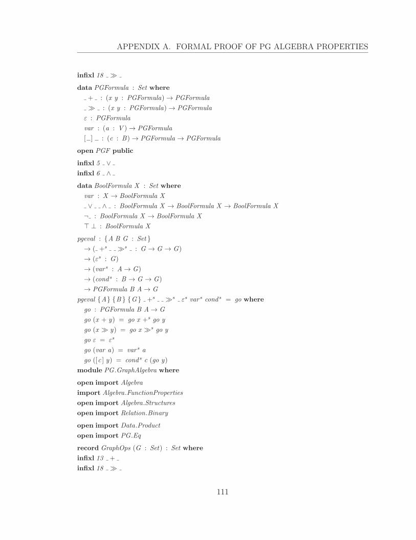
APPENDIX A. FORMAL PROOF OF PG ALGEBRA PROPERTIES
infixl 18 ≫
data PGFormula : Set where
+ : (x y : PGFormula) → PGFormula
≫ : (x y : PGFormula) → PGFormula
ε : PGFormula
var : (a : V ) → PGFormula
[ ] : (c : B) → PGFormula → PGFormula
open PGF public
infixl 5 ∨
infixl 6 ∧
data BoolFormula X : Set where
var : X → BoolFormula X
∨ ∧ : BoolFormula X → BoolFormula X → BoolFormula X
¬ : BoolFormula X → BoolFormula X
⊤ ⊥ : BoolFormula X
pgeval : {A B G : Set }
→ ( +s ≫s : G → G → G)
→ (εs : G)
→ (var s : A → G)
→ (cond s : B → G → G)
→ PGFormula B A → G
pgeval {A} {B } {G } +s ≫s εs var s cond s = go where
go : PGFormula B A → G
go (x + y) = go x +s go y
go (x ≫ y) = go x ≫s go y
go ε = εs
go (var a) = var s a
go ([c ] y) = cond s c (go y)
module PG .GraphAlgebra where
open import Algebra
import Algebra.FunctionProperties
open import Algebra.Structures
open import Relation.Binary
open import Data.Product
open import PG .Eq
record GraphOps (G : Set) : Set where
infixl 13 +
infixl 18 ≫
111

APPENDIX A. FORMAL PROOF OF PG ALGEBRA PROPERTIES
field
+ : (p q : G) → G
≫ : (p q : G) → G
ε : G
record IsGraph {G : Set } (Eq : Eq G) (Ops : GraphOps G) : Set where
open GraphOps Ops
open Eq Eq renaming ( ≈ to ≈ )
field
+cong : ∀ {p q r s } → p ≈ r → q ≈ s → p + q ≈ r + s
≫ cong : ∀ {p q r s } → p ≈ r → q ≈ s → p ≫ q ≈ r ≫ s
≈ iseq : IsEquivalence ≈
+assoc : ∀ {p q r } → (p + q) + r ≈ p + (q + r)
+comm : ∀ {p q } → p + q ≈ q + p
≫ assoc : ∀ {p q r } → (p ≫ q) ≫ r ≈ p ≫ (q ≫ r)
≫ identity l : ∀ {p} → ε ≫ p ≈ p
≫ identityr : ∀ {p} → p ≫ ε ≈ p
distribl : {p q r : G } → p ≫ (q + r) ≈ p ≫ q + p ≫ r
distribr : {p q r : G } → (p + q) ≫ r ≈ p ≫ r + q ≫ r
decomposition : {p q r : G } → p ≫ q ≫ r ≈ p ≫ q + p ≫ r + q ≫ r
open IsEquivalence ≈ iseq public
record Graph (G : Set) : Set1 where
field
eq : Eq G
ops : GraphOps G
isGraph : IsGraph eq ops
open IsGraph isGraph public
open Eq eq public
open GraphOps ops public
import Level
open Level using () renaming (zero to 0 )
import Relation.Binary .EqReasoning
open import Function
open import Data.List hiding ([ ])
import Relation.Binary .PropositionalEquality
module GraphTheory {P : Set } (graph : Graph P) where
open Graph graph
open Relation.Binary .EqReasoning record {isEquivalence = ≈ iseq }
open import Relation.Binary
112
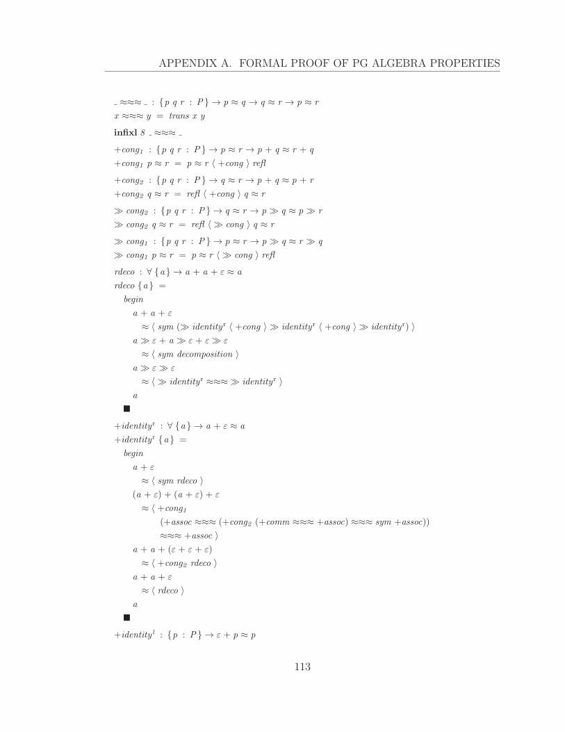
APPENDIX A. FORMAL PROOF OF PG ALGEBRA PROPERTIES
≈≈≈ : {p q r : P } → p ≈ q → q ≈ r → p ≈ r
x ≈≈≈ y = trans x y
infixl 8 ≈≈≈
+cong1 : {p q r : P } → p ≈ r → p + q ≈ r + q
+cong1 p ≈ r = p ≈ r 〈 +cong 〉 refl
+cong2 : {p q r : P } → q ≈ r → p + q ≈ p + r
+cong2 q ≈ r = refl 〈 +cong 〉 q ≈ r
≫ cong2 : {p q r : P } → q ≈ r → p ≫ q ≈ p ≫ r
≫ cong2 q ≈ r = refl 〈 ≫ cong 〉 q ≈ r
≫ cong1 : {p q r : P } → p ≈ r → p ≫ q ≈ r ≫ q
≫ cong1 p ≈ r = p ≈ r 〈 ≫ cong 〉 refl
rdeco : ∀ {a } → a + a + ε ≈ a
rdeco {a } =
begin
a + a + ε
≈ 〈 sym (≫ identityr 〈 +cong 〉 ≫ identityr 〈 +cong 〉 ≫ identityr) 〉
a ≫ ε + a ≫ ε + ε ≫ ε
≈ 〈 sym decomposition 〉
a ≫ ε ≫ ε
≈ 〈 ≫ identityr ≈≈≈ ≫ identityr 〉
a
�
+identityr : ∀ {a } → a + ε ≈ a
+identityr {a } =
begin
a + ε
≈ 〈 sym rdeco 〉
(a + ε) + (a + ε) + ε
≈ 〈 +cong1
(+assoc ≈≈≈ (+cong2 (+comm ≈≈≈ +assoc) ≈≈≈ sym +assoc))
≈≈≈ +assoc 〉
a + a + (ε + ε + ε)
≈ 〈 +cong2 rdeco 〉
a + a + ε
≈ 〈 rdeco 〉
a
�
+identity l : {p : P } → ε + p ≈ p
113
APPENDIX A. FORMAL PROOF OF PG ALGEBRA PROPERTIES
+identity l = +comm ≈≈≈ +identityr
idempotence : ∀ {p} → p + p ≈ p
idempotence {p} = sym +identityr ≈≈≈ rdeco
absorption : ∀ {a b} → a ≫ b + a + b ≈ a ≫ b
absorption {a } {b} =
begin
a ≫ b + a + b
≈ 〈 sym (refl 〈 +cong 〉 ≫ identityr 〈 +cong 〉 ≫ identityr) 〉
(a ≫ b) + (a ≫ ε) + (b ≫ ε)
≈ 〈 sym decomposition 〉
a ≫ b ≫ ε
≈ 〈 ≫ identityr 〉
a ≫ b
�
absorption l : {p q : P } → p ≫ q + p ≈ p ≫ q
absorption l {p} {q } =
begin
p ≫ q + p
≈ 〈 +cong1 (sym absorption) 〉
p ≫ q + p + q + p
≈ 〈 +assoc ≈≈≈ +cong2 +comm ≈≈≈ (sym +assoc ≈≈≈ +cong1 +assoc) 〉
p ≫ q + (p + p) + q
≈ 〈 +cong1 (+cong2 idempotence) 〉
p ≫ q + p + q
≈ 〈 absorption 〉
p ≫ q
�
absorptionr : ∀ {p} {q } → p ≫ q + q ≈ p ≫ q
absorptionr {p} {q } =
begin
p ≫ q + q
≈ 〈 +cong1 (sym absorption) 〉
p ≫ q + p + q + q
≈ 〈 +assoc 〉
p ≫ q + p + (q + q)
≈ 〈 +cong2 idempotence 〉
p ≫ q + p + q
≈ 〈 absorption 〉
p ≫ q
114

APPENDIX A. FORMAL PROOF OF PG ALGEBRA PROPERTIES
�
⊆ : (p q : P) → Set
p ⊆ q = p + q ≈ q
infix 10 ⊆
leastElement : {p : P } → ε ⊆ p
leastElement = +identity l
p + q ⊆ p ≫ q : {p q : P } → p + q ⊆ p ≫ q
p + q ⊆ p ≫ q = +comm ≈≈≈ sym +assoc ≈≈≈ absorption
⊆ refl0 : {p : P } → p ⊆ p
⊆ refl0 = idempotence
⊆ refl : {p q : P } → p ≈ q → p ⊆ q
⊆ refl p ≈ q = +cong1 p ≈ q ≈≈≈ idempotence
⊆ antisym : {p q : P } → p ⊆ q → q ⊆ p → p ≈ q
⊆ antisym p + q ≈ q q + p ≈ p = sym (+comm ≈≈≈ q + p ≈ p) ≈≈≈ p + q ≈ q
⊆ trans : {p q r : P } → p ⊆ q → q ⊆ r → p ⊆ r
⊆ trans {p} {q } {r } p + q ≈ q q + r ≈ r =
begin
p + r
≈ 〈 sym (+assoc ≈≈≈ +cong2 q + r ≈ r) 〉
p + q + r
≈ 〈 +cong1 p + q ≈ q ≈≈≈ q + r ≈ r 〉
r
�
⊆ isPartialOrder : IsPartialOrder ≈ ⊆
⊆ isPartialOrder = record
{isPreorder = record
{isEquivalence = ≈ iseq
; trans = ⊆ trans
; reflexive = ⊆ refl
}
; antisym = ⊆ antisym
}
+isSemigroup : IsSemigroup ≈ +
+isSemigroup = record
{isEquivalence = ≈ iseq
; assoc = λ x y z → +assoc {x } {y } {z }
; •cong = +cong
115
APPENDIX A. FORMAL PROOF OF PG ALGEBRA PROPERTIES
}
+isCommutativeMonoid : IsCommutativeMonoid ≈ + ε
+isCommutativeMonoid = record
{isSemigroup = +isSemigroup
; identity l = λ x → +identity l {x }
; comm = λ x y → +comm {x } {y }
}
≫ isSemigroup : IsSemigroup ≈ ≫
≫ isSemigroup = record
{isEquivalence = ≈ iseq
; assoc = λ x y z → ≫ assoc {x } {y } {z }
; •cong = ≫ cong
}
≫ isMonoid : IsMonoid ≈ ≫ ε
≫ isMonoid = record
{isSemigroup = ≫ isSemigroup
; identity = (λ x → ≫ identity l {x }), (λ x → ≫ identityr {x })
}
cpogIsSemiringWithoutAnnihilatingZero
: IsSemiringWithoutAnnihilatingZero ≈ + ≫ ε ε
cpogIsSemiringWithoutAnnihilatingZero = record
{+isCommutativeMonoid = +isCommutativeMonoid
; ∗isMonoid = ≫ isMonoid
; distrib = (λ → distribl), (λ → distribr)
}
+monotony : {p q r s : P } → p ⊆ q → r ⊆ s → p + r ⊆ q + s
+monotony {p} {q } {r } {s } p + q ≈ q r + s ≈ s =
begin
(p + r) + (q + s)
≈ 〈 sym +assoc ≈≈≈
+cong1 (+assoc ≈≈≈ +cong2 +comm ≈≈≈ sym +assoc)
≈≈≈ +assoc 〉
(p + q) + (r + s)
≈ 〈 p + q ≈ q 〈 +cong 〉 r + s ≈ s 〉
q + s
�
+preserves ⊆ : + Preserves2 ⊆ −→ ⊆ −→ ⊆
+preserves ⊆ = +monotony
116
APPENDIX A. FORMAL PROOF OF PG ALGEBRA PROPERTIES
≫ arg1Monotony : {p q r : P } → p ⊆ q → p ≫ r ⊆ q ≫ r
≫ arg1Monotony p + q ≈ q = sym distribr ≈≈≈ ≫ cong1 p + q ≈ q
≫ arg2Monotony : {p r s : P } → r ⊆ s → p ≫ r ⊆ p ≫ s
≫ arg2Monotony r + s ≈ s = sym distribl ≈≈≈ ≫ cong2 r + s ≈ s
≫ monotony : {p q r s : P } → p ⊆ q → r ⊆ s → p ≫ r ⊆ q ≫ s
≫ monotony p + q ≈ q r + s ≈ s = ⊆ trans (≫ arg1Monotony p + q ≈ q) (≫ arg2Monotony r + s ≈ s)
≫ preserves ⊆ : ≫ Preserves2 ⊆ −→ ⊆ −→ ⊆
≫ preserves ⊆ = ≫ monotony
module PG .Normalizercorrect (A B : Set) where
open import Relation.Binary
import Relation.Binary .PropositionalEquality as PropEq
open PropEq using ( ≡ )
open import PG .Formulae
module WithOrder { < : A → A → Set } (ASTO : IsStrictTotalOrder ≡ < ) where
open import PG .FormulaEq
import PG .Normalizer
open PG .Normalizer .WithOrder A B ASTO renaming ( + to +′ ; ≫ to ≫′ )
open PG .Normalizer A B
import Data.List as List
open List using ([ ]; : : ; foldr ;map)
open import Function
open WithBV {B } {A}
import PG .GraphAlgebra as Alg
module GT = Alg .GraphTheory (record {isGraph = pgformulaisgraph })
module BEq = IsEquivalence B ≈ isequivalence
open IsEquivalence ≈ isequivalence
import Relation.Binary .EqReasoning as EqR
open EqR record {isEquivalence = ≈ isequivalence }
open EqR record {isEquivalence = B ≈ isequivalence } renaming
(begin to Bbegin ; ≈ 〈 〉 to B ≈ 〈 〉 ; � to B�)
open import Algebra.Structures
open IsBooleanAlgebra boolformulaisboolalg using
()
open import Algebra.Props .BooleanAlgebra
(record {isBooleanAlgebra = boolformulaisboolalg }) using
(∧ ∨ distrib;∧complement ;∨complement ;
∨ ∧ isCommutativeSemiring ;∧idempotent ;∨idempotent)
open IsCommutativeSemiring ∨ ∧ isCommutativeSemiring
117
APPENDIX A. FORMAL PROOF OF PG ALGEBRA PROPERTIES
using () renaming (∗identity to ∧identity ; zero to ∧zero)
open import Data.Product using ( , ; proj1 ; proj2 )
open import Data.Sum using (inj1 ; inj2 )
absorption : ∀ {x y } → x + y + x ≫ y ≈ x ≫ y
absorption = +comm 〈 trans 〉 (sym +assoc 〈 trans 〉 GT .absorption)
lem : ∀ f p → p ≈ [f ] p + [¬ f ] p
lem f p =
begin
p
≈ 〈 sym truecondition 〉
[⊤ ] p
≈ 〈 condcong (isEquivalence (EQC .sym ∨complement r)) refl 〉
[f ∨ ¬ f ] p
≈ 〈 orcondition 〉
[f ] p + [¬ f ] p
�
caseanalyse : ∀ {f p q } → [f ] p ≈ [f ] q → [¬ f ] p ≈ [¬ f ] q → p ≈ q
caseanalyse {f } {p} {q } fcase ¬fcase =
begin
p
≈ 〈 lem 〉
[f ] p + [¬ f ] p
≈ 〈 +cong fcase ¬fcase 〉
[f ] q + [¬ f ] q
≈ 〈 sym (lem ) 〉
q
�
elim+ : ∀ {f a b c d }
→ [f ] a ≈ [f ] c → [f ] b ≈ [f ] d
→ [f ] (a + b) ≈ [f ] (c + d)
elim+ a ≈ c b ≈ d =
trans (trans conditional+ (+cong a ≈ c b ≈ d)) (sym conditional+)
elim ≫ : ∀ {f a b c d } →
[f ] a ≈ [f ] c → [f ] b ≈ [f ] d →
[f ] (a ≫ b) ≈ [f ] (c ≫ d)
elim ≫ a ≈ c b ≈ d =
trans (trans conditional ≫ (≫ cong a ≈ c b ≈ d)) (sym conditional ≫)
dupcond : ∀ {f x } → [f ] [f ] x ≈ [f ] x
118
APPENDIX A. FORMAL PROOF OF PG ALGEBRA PROPERTIES
dupcond = trans (sym andcondition) (condcong (∧idempotent ) refl)
falsecond : ∀ {f x } → [¬ f ] [f ] x ≈ [¬ f ] ε
falsecond = trans (sym dupcond) (condcong BEq .refl (trans
(trans (sym andcondition)
(condcong (proj1 ∧complement ) refl))
falsecondition
)
)
condswap : ∀ {f g x } → [f ] [g ] x ≈ [g ] [f ] x
condswap = trans (sym andcondition) (trans (condcong ∧comm refl) andcondition)
side1 : ∀ {f g p q }
→ [f ] ([f ] p ≫ [g ] q)
≈ [f ] ([f ] p + [g ] q + [f ∧ g ] (p ≫ q))
side1 {f } {g } {p} {q } =
begin
[f ] ([f ] p ≫ [g ] q)
≈ 〈 elim ≫ dupcond refl 〉
[f ] (p ≫ [g ] q)
≈ 〈 condcong BEq .refl (caseanalyse {g }
(
begin
[g ] (p ≫ [g ] q)
≈ 〈 elim ≫ refl dupcond 〉
[g ] (p ≫ q)
≈ 〈 sym (condcong BEq .refl absorption) 〉
[g ] (p + q + p ≫ q)
≈ 〈 sym (elim+ (elim+ refl dupcond) dupcond) 〉
[g ] (p + [g ] q + [g ] (p ≫ q))
�
)
(trans (elim ≫ refl falsecond) (trans
(condcong BEq .refl
(trans ≫ identityr (sym (trans GT .+ identityr GT .+ identityr))))
(sym (elim+ (elim+ refl falsecond) falsecond))))) 〉
[f ] (p + [g ] q + [g ] (p ≫ q))
≈ 〈 sym (elim+ (elim+ dupcond refl)
(trans (condcong BEq .refl andcondition) dupcond)) 〉
[f ] ([f ] p + [g ] q + [f ∧ g ] (p ≫ q))
�
119
APPENDIX A. FORMAL PROOF OF PG ALGEBRA PROPERTIES
side2 : ∀ {f g p q }
→ [¬ f ] ([f ] p ≫ [g ] q)
≈ [¬ f ] ([f ] p + [g ] q + [f ∧ g ] (p ≫ q))
side2 {f } {g } {p} {q } =
begin
[¬ f ] ([f ] p ≫ [g ] q)
≈ 〈 elim ≫ falsecond refl 〉
[¬ f ] (ε ≫ [g ] q)
≈ 〈 condcong BEq .refl ≫ identity l 〉
[¬ f ] [g ] q
≈ 〈 condcong BEq .refl (sym (trans (GT .+ identityr) (GT .+ identity l))) 〉
[¬ f ] (ε + [g ] q + ε)
≈ 〈 sym (elim+ (elim+ falsecond refl) (trans (sym dupcond)
(condcong BEq .refl (trans (sym andcondition)
(trans (condcong (BEq .trans (BEq .sym ∧assoc)
(BEq .trans (∧cong (proj1 ∧complement ) BEq .refl) (proj1 ∧zero )))
refl) falsecondition))))) 〉
[¬ f ] ([f ] p + [g ] q + [f ∧ g ] (p ≫ q))
�
conditionregularisation : ∀ {f g } → {p q : PG }
→ [f ] p ≫ [g ] q ≈ [f ] p + [g ] q + [f ∧ g ] (p ≫ q)
conditionregularisation {f } {g } {p} {q } = caseanalyse {f }
side1 side2
absorbbycondition : ∀ {f g p} → [f ] p + [f ∧ g ] p ≈ [f ] p
absorbbycondition {f } {g } {p} =
sym orcondition 〈 trans 〉 condcong ∨absorbs∧ refl
conditionregularisation ′ : ∀ f g p q z
→ p ≫ q ≈ p + q + z
→ [f ] p ≫ [g ] q
≈ [f ] p + [g ] q + [f ∧ g ] z
conditionregularisation ′ f g p q z eq =
begin
[f ] p ≫ [g ] q
≈ 〈 conditionregularisation 〉
[f ] p + [g ] q + [f ∧ g ] (p ≫ q)
≈ 〈 +cong refl (condcong (isEquivalence EQC .refl) eq) 〉
[f ] p + [g ] q + [f ∧ g ] (p + q + z )
≈ 〈 +cong refl (conditional+ 〈 trans 〉 +cong conditional+ refl) 〉
[f ] p + [g ] q + ([f ∧ g ] p + [f ∧ g ] q + [f ∧ g ] z )
120
APPENDIX A. FORMAL PROOF OF PG ALGEBRA PROPERTIES
≈ 〈 sym +assoc 〈 trans 〉 +cong (+assoc 〈 trans 〉
(+cong refl (sym +assoc 〈 trans 〉 +cong +comm refl 〈 trans 〉 +assoc)
〈 trans 〉 sym +assoc)) refl 〉
([f ] p + [f ∧ g ] p) + ([g ] q + [f ∧ g ] q) + [f ∧ g ] z
≈ 〈 +cong (+cong absorbbycondition (+cong refl (condcong ∧comm refl)
〈 trans 〉 absorbbycondition)) refl 〉
[f ] p + [g ] q + [f ∧ g ] z
�
+correct ′ : ∀ x y → fromNF x + fromNF y ≈ fromNF (x +′ y)
+correct ′ [ ] y = GT .+ identity l (fromNF y)
+correct ′ (x : : xs) y = +assoc 〈 trans 〉 +cong refl (+correct ′ xs y)
sumNodes = foldr + ε ◦ map fromNode
absorption l : ∀ {x y } → x + x ≫ y ≈ x ≫ y
absorption l = +comm 〈 trans 〉 GT .absorption l
absorptionr : ∀ {x y } → y + x ≫ y ≈ x ≫ y
absorptionr = +comm 〈 trans 〉 GT .absorptionr
newArrowsgood : ∀ x y → fromNode x ≫ fromNode y
≈ fromNode x + fromNode y + sumNodes (newArrows x y)
newArrowsgood (inj1 x ) (inj1 y) =
sym (+cong refl GT .+ identityr 〈 trans 〉 absorption)
newArrowsgood (inj1 x ) (inj2 (y1 , y2 )) =
sym (+cong +comm (+cong refl GT .+ identityr)
〈 trans 〉 (+assoc 〈 trans 〉 +comm 〈 trans 〉
+cong (sym +assoc 〈 trans 〉 +cong absorption l refl) refl)
〈 trans 〉 sym decomposition
〈 trans 〉 ≫ assoc)
newArrowsgood (inj2 (x1 , x2 )) (inj1 y) =
sym (+assoc 〈 trans 〉
+cong refl (sym +assoc 〈 trans 〉 +cong absorptionr GT .+ identityr)
〈 trans 〉 sym +assoc 〈 trans 〉
sym decomposition)
newArrowsgood (inj2 (x1 , x2 )) (inj2 (y1 , y2 )) =
sym (+assoc 〈 trans 〉 +cong refl
(+cong (sym GT .idempotence) (+cong refl (+cong refl
(+cong refl GT .+ identityr)) 〈 trans 〉 sym +assoc 〈 trans 〉 +comm)
〈 trans 〉 sym +assoc
〈 trans 〉 +cong (+assoc 〈 trans 〉 +cong refl +comm) refl
〈 trans 〉 +comm
〈 trans 〉 sym +assoc
121
APPENDIX A. FORMAL PROOF OF PG ALGEBRA PROPERTIES
〈 trans 〉 +cong (sym decomposition) (sym decomposition)
〈 trans 〉 +cong ≫ assoc ≫ assoc
)
〈 trans 〉 sym +assoc
〈 trans 〉 sym decomposition)
allmult : ∀ l c → fromNF (List .map (flip , c) l) ≈ [c ] sumNodes l
allmult [ ] c = sym conditionalε
allmult (x : : xs) c = +cong refl (allmult xs c) 〈 trans 〉 sym conditional+
≫1 preserves : ∀ x y → fromLit x ≫ fromLit y ≈ fromNF (x ≫1 y)
≫1 preserves (x , f ) (y , g) =
begin
fromLit (x , f ) ≫ fromLit (y , g)
≈ 〈 conditionregularisation ′ f g (newArrowsgood x y) 〉
fromLit (x , f ) + fromLit (y , g) + [f ∧ g ] sumNodes (newArrows x y)
≈ 〈 +assoc 〈 trans 〉 +cong refl
(+cong refl (sym (allmult (newArrows x y) (f ∧ g)))) 〉
fromNF ((x , f ) : : (y , g) : : (map (flip , (f ∧ g)) (newArrows x y)))
≈ 〈 refl 〉
fromNF ((x , f ) ≫1 (y , g))
�
≫ rpreserves : ∀ x y → fromLit x ≫ fromNF y ≈ fromNF (x ≫ r y)
≫ rpreserves x [ ] = ≫ identityr 〈 trans 〉 sym GT .+ identityr
≫ rpreserves x (y : : ys) =
distribl 〈 trans 〉 +cong (≫1 preserves x y) (≫ rpreserves x ys)
〈 trans 〉 +correct ′ (x ≫1 y) (x ≫ r ys)
≫ correct ′ : ∀ x y → fromNF x ≫ fromNF y ≈ fromNF (x ≫′ y)
≫ correct ′ [ ] y = ≫ identity l
≫ correct ′ (x : : xs) y =
distribr 〈 trans 〉 (+cong (≫ rpreserves x y) (≫ correct ′ xs y)
〈 trans 〉 +correct ′ (x ≫ r y) (xs ≫′ y))
+correct : ∀ x y → x + y ≈ fromNF (normalize x +′ normalize y)
≫ correct : ∀ x y → x ≫ y ≈ fromNF (normalize x ≫′ normalize y)
normalisecorrect : ∀ f → f ≈ fromNF (normalize f )
+correct x y =
+cong (normalisecorrect x ) (normalisecorrect y) 〈 trans 〉
+correct ′ (normalize x ) (normalize y)
≫ correct x y =
≫ cong (normalisecorrect x ) (normalisecorrect y) 〈 trans 〉
122
APPENDIX A. FORMAL PROOF OF PG ALGEBRA PROPERTIES
≫ correct ′ (normalize x ) (normalize y)
mapConditionscorrect : ∀ c x → [c ] fromNF x ≈ fromNF (mapConditions ( ∧ c) x )
mapConditionscorrect c [ ] = conditionalε
mapConditionscorrect c (x : : xs) =
conditional+ 〈 trans 〉 +cong (sym andcondition) (mapConditionscorrect c xs)
normalisecorrect (x + y) = +correct x y
normalisecorrect (x ≫ y) = ≫ correct x y
normalisecorrect ε = refl
normalisecorrect (var a) = sym truecondition 〈 trans 〉 sym GT .+ identityr
normalisecorrect ([c ] y) = condcong BEq .refl (normalisecorrect y) 〈 trans 〉
mapConditionscorrect c (normalize y)
module PG .Normalizer (V : Set) (B : Set) where
open import Data.Empty
open import Data.Sum using ( ⊎ ; inj1 ; inj2 )
open import Function using (id ;flip; ◦ )
import Data.Product as Product
open Product using ( , ; × )
open import Level using () renaming (zero to 0 )
open import PG .Formulae using
(BoolFormula; ∧ ; ∨ ;⊤; var ;PGFormula;module PGFormula; pgeval)
open import Relation.Binary
open import Relation.Binary .PropositionalEquality using ( ≡ )
import Data.List as List
open List using (foldr ;List ; concat ; + + ; : : ; [ ];map)
BF = BoolFormula B
PG = PGFormula BF V
Node = V ⊎ (V × V )
Lit = Node × BF
NF = List Lit
module WithOrder { < : V → V → Set } (ASTO : IsStrictTotalOrder ≡ < ) where
module Semantics where
open PGFormula
fromNode : Node → PG
fromNode (inj1 x ) = var x
fromNode (inj2 (x , y)) = var x ≫ var y
fromLit : Lit → PG
fromLit (node, cond) = [cond ] fromNode node
123
APPENDIX A. FORMAL PROOF OF PG ALGEBRA PROPERTIES
fromNF : NF → PG
fromNF = foldr + ε ◦ map fromLit
open Semantics public
open import Category .Monad
open RawMonad (List .monad {0 })
+ : NF → NF → NF
a + b = a ++ b
vertices : Node → List V
vertices (inj1 x ) = x : : [ ]
vertices (inj2 (x , y)) = x : : y : : [ ]
newArrows : Node → Node → List Node
newArrows p q = map inj2 (vertices p ⊗ vertices q)
≫1 : Lit → Lit → List Lit
(p, f ) ≫1 (q , g) =
(p, f ) : : (q , g) : : (map (flip , (f ∧ g)) (newArrows p q))
≫ r : Lit → NF → NF
lit ≫ r [ ] = lit : : [ ]
lit ≫ r (x : : xs) = (lit ≫1 x ) + (lit ≫ r xs)
≫ : NF → NF → NF
[ ] ≫ b = b
(h : : t) ≫ b = (h ≫ r b) + (t ≫ b)
mapConditions : (BF → BF ) → NF → NF
mapConditions f = map (Product .map id f )
fromVar : V → NF
fromVar x = (inj1 x ,⊤) : : [ ]
addCondition : BF → NF → NF
addCondition = mapConditions ◦ ∧
normalize : PG → NF
normalize = pgeval
+
≫
[ ]
fromVar
addCondition
open import PG .PGAlgebra using (BoolOps)
module PG .PGAlgebra where
124
APPENDIX A. FORMAL PROOF OF PG ALGEBRA PROPERTIES
open import PG .GraphAlgebra
open import PG .Eq
open import Algebra.Structures
record BoolOps (B : Set) : Set where
infix 8 ¬
infixr 7 ∧
infixr 6 ∨
field
∨ : B → B → B
∧ : B → B → B
¬ : B → B
⊤ : B
⊥ : B
record PGOps (B G : Set) : Set where
infix 20 [ ]
field
graphops : GraphOps G
[ ] : B → G → G
open GraphOps graphops public
IsBoolAlg : {B : Set } → (Beq : Eq B) → (boolops : BoolOps B) → Set
IsBoolAlg (equality eq) ops = let open BoolOps ops in
IsBooleanAlgebra eq ∨ ∧ ¬ ⊤ ⊥
record IsPG {B G : Set }
(Beq : Eq B) (Geq : Eq G)
(PGops : PGOps B G) (Bops : BoolOps B) : Set where
open PGOps PGops
open Eq Geq
open Eq Beq renaming ( ≈ to B ≈ )
open BoolOps Bops
field
isgraph : IsGraph Geq graphops
isbool : IsBoolAlg Beq Bops
condcong : ∀ {f g x y } → f B ≈ g → x ≈ y → [f ] x ≈ [g ] y
truecondition : ∀ x → [⊤ ] x ≈ x
falsecondition : ∀ x → [⊥ ] x ≈ ε
andcondition : ∀ f g x → [f ∧ g ] x ≈ [f ] [g ] x
orcondition : ∀ f g x → [f ∨ g ] x ≈ [f ] x + [g ] x
conditional+ : ∀ f x y → [f ] (x + y) ≈ [f ] x + [f ] y
125
APPENDIX A. FORMAL PROOF OF PG ALGEBRA PROPERTIES
conditional ≫ : ∀ f x y → [f ] (x ≫ y) ≈ [f ] x ≫ [f ] y
open PGOps PGops public
open Eq Geq public
open IsGraph isgraph public
open IsBooleanAlgebra isbool public using ()
open BoolOps Bops public
record PG (B G : Set) : Set1 where
field
Beq : Eq B
Geq : Eq G
pgops : PGOps B G
Bops : BoolOps B
isPg : IsPG Beq Geq pgops Bops
open IsPG isPg public
126

Bibliography
[1] MSP430x4xx Family User’s Guide.
[2] International technology roadmap for semiconductors: 2011 edition.
http://www.itrs.net/Links/2011ITRS/Home2011.htm, 2011.
[3] Arseniy Alekseyev, Victor Khomenko, Andrey Mokhov, Dominic Wist, and Alex
Yakovlev. Improved parallel composition of labelled Petri nets. In Benoıt Cail-
laud, Josep Carmona, and Kunihiko Hiraishi, editors, ACSD, pages 131–140.
IEEE, 2011.
[4] Arseniy Alekseyev, Ivan Poliakov, Victor Khomenko, and Alex Yakovlev. Op-
timisation of Balsa control path using STG resynthesis. In UK Asynchronous
Forum, 2009.
[5] Thorsten Altenkirch and Peter Morris. Indexed containers. In LICS, pages
277–285. IEEE Computer Society, 2009.
[6] Samary I. Baranov. Logic Synthesis for Control Automata. Kluwer Academic
Publishers, 1994.
[7] Kees van Berkel. Handshake Circuits: An Asynchronous Architecture for VLSI
Programming. Cambridge International Series on Parallel Computation. Cam-
bridge University Press, 2004.
[8] Kees van Berkel, Joep Kessels, Marly Roncken, Ronald Saeijs, and Frits Schalij.
The VLSI-programming language Tangram and its translation into handshake
circuits. In Proc. European Conference on Design Automation (EDAC), 1991.
127
BIBLIOGRAPHY
[9] Ales Bizjak and Andrej Bauer. Alg User Manual, Faculty of Mathematics and
Physics, University of Ljubljana, 2011.
[10] Daniel M. Chapiro. Globally-Asynchronous Locally-Synchronous systems. PhD
thesis, Stanford University, October 1984.
[11] Tiberiu Chelcea and Steven M. Nowick. Resynthesis and peephole transforma-
tions for the optimization of large-scale asynchronous systems. In Proc. DAC’02,
pages 405–410, 2002.
[12] Clasp tool. URL: http://www.cs.uni-potsdam.de/clasp/.
[13] Jordi Cortadella, Michael Kishinevsky, Alex Kondratyev, Luciano Lavagno, and
Alex Yakovlev. Petrify: a tool for manipulating concurrent specifications and
synthesis of asynchronous controllers. IEICE Trans. Information and Systems,
E80-D, 3:315–325, 1997.
[14] Jordi Cortadella, Michael Kishinevsky, Alex Kondratyev, Luciano Lavagno, and
Alex Yakovlev. Logic synthesis of asynchronous controllers and interfaces. Ad-
vanced Microelectronics. Springer-Verlag, 2002.
[15] Jordi Cortadella, Alex Kondratyev, Luciano Lavagno, and Christos Sotiriou.
Desynchronisation: synthesis of asynchronous circuits from synchronous spe-
cifications. IEEE Transaction on Computer Aided Design, 25(10):1904–1921,
October 2006.
[16] Jordi Cortadella, Luciano Lavagno, Djavad Amiri, Jon‘as Casanova, Carlos
Macian, Ferran Martorell, Juan A. Moya, Luca Necchi, Danil Sokolov, and Emre
Tuncer. Narrowing the margins with elastic clocks. In IEEE International Con-
ference on Integrated Circuit Design and Technology (ICICDT), pages 146–150,
2010.
[17] Crescenzo D’Alessandro, Andrey Mokhov, Alexander Bystrov, and Alex
Yakovlev. Delay/phase regeneration circuits. In 13th IEEE International Sym-
posium on Asynchronous Circuits and Systems (ASYNC), 2007, pages 105–116,
March 2007.
128

BIBLIOGRAPHY
[18] Nils Anders Danielsson. Agda standard library. http://wiki.portal.
chalmers.se/agda/agda.php?n=Libraries.StandardLibrary, 2011.
[19] Giovanni de Micheli. Synthesis and Optimization of Digital Circuits. McGraw-
Hill Higher Education, 1994.
[20] Jo C. Ebergen. Arbiters: an exercise in specifying and decomposing asynchron-
ously communicating components. Sci. of Computer Programming, 18:223–245,
1992.
[21] Doug A. Edwards and Andrew Bardsley. Balsa: an Asynchronous Hardware
Synthesis Language. The Computer Journal, 45(1):12–18, 2002.
[22] Doug A. Edwards and Andrew Bardsley. Balsa: An asynchronous hardware
synthesis language. The Computer Journal, 45 (1):12–18, jan 2002.
[23] Niklas Een and Niklas Sorensson. An Extensible SAT-solver. Theory and Ap-
plications of Satisfiability Testing, pages 333–336, 2004.
[24] Xin Fan, Milos Krstic, and Eckhard Grass. Analysis and optimization of pausible
clocking based gals design. In IEEE International Conference on Computer
Design (ICCD), pages 358–365, 2009.
[25] Francisco Fernandez-Nogueira and Josep Carmona. Logic synthesis of hand-
shake components using structural clustering techniques. In Lars Svensson and
Jose Monteiro, editors, Integrated Circuit and System Design. Power and Tim-
ing Modeling, Optimization and Simulation, volume 5349 of Lecture Notes in
Computer Science, pages 188–198. Springer Berlin Heidelberg, 2009.
[26] Charles Antony Richard Hoare. Communicating sequential processes. Prentice-
Hall, Inc., Upper Saddle River, NJ, USA, 1985.
[27] Alan Jeffrey. LTL types FRP: linear-time temporal logic propositions as types,
proofs as functional reactive programs. In Koen Claessen and Nikhil Swamy,
editors, PLPV, pages 49–60. ACM, 2012.
[28] Mark B. Josephs and Dennis Furey. Delay-insensitive interface specification and
synthesis. In Proc. DATE’00, pages 169–173, 2000.
129
BIBLIOGRAPHY
[29] Joep Kessels and Ad Peeters. The tangram framework: asynchronous circuits
for low power. In Design Automation Conference, 2001. Proceedings of the
ASP-DAC 2001. Asia and South Pacific, pages 255–260, 2001.
[30] Victor Khomenko, Maciej Koutny, and Alex Yakovlev. Detecting state encoding
conflicts in STG unfoldings using SAT. Fundam. Inf., 62(2):221–241, 2004.
[31] Victor Khomenko, Mark Schafer, and Walter Vogler. Output-determinacy and
asynchronous circuit synthesis. Fundamenta Informaticae, 88(4):541–579, 2008.
Special Issue on Best Papers from ACSD’07.
[32] Victor Khomenko, Mark Schafer, Walter Vogler, and Ralf Wollowski. STG
decomposition strategies in combination with unfolding. Acta Informatica,
46(6):433–474, 2009.
[33] Tilman Kolks, Steven Vercauteren, and Bill Lin. Control resynthesis for control-
dominated asynchronous designs. Proc. ASYNC’96, pages 233–243, 1996.
[34] Alex Kondratyev and Kelvin Lwin. Design of asynchronous circuits using syn-
chronous cad tools. IEEE Design & Test of Computers, 19(4):107–117, 2002.
[35] Jong-eun Lee, Kiyoung Choi, and Nikil Dutt. Efficient instruction encoding for
automatic instruction set design of configurable asips. In Proc. of the Interna-
tional Conference on Computer-aided Design (ICCAD), 2002.
[36] Alain J. Martin and Mika Nystrom. Asynchronous techniques for system-on-
chip design. IEEE Proceedings, 94:1089–1120, 2006.
[37] Ross M. McConnell and Fabien de Montgolfier. Linear-time modular decompos-
ition of directed graphs. Discrete Applied Mathematics, 145(2):198–209, 2005.
[38] Prabhat Mishra and Nikil Dutt. Processor Modelling and Design Tools, Chapter
8 in ‘EDA for IC Systems Design, Verification, and Testing’ by L. Sheffer, L.
Lavagno, and G. Martin. Taylor and Francis Group, 2006.
[39] Andrey Mokhov. Conditional Partial Order Graphs. PhD thesis, Newcastle
University, 2009.
130
BIBLIOGRAPHY
[40] Andrey Mokhov, Arseniy Alekseyev, and Alex Yakovlev. Encoding of processor
instruction sets with explicit concurrency control. IET Computers & Digital
Techniques, 5(6):427–439, 2011.
[41] Andrey Mokhov, Alexei Iliasov, Danil Sokolov, Maxim Rykunov, Alex Yakovlev,
and Alexander Romanovsky. Synthesis of processor instruction sets from high-
level ISA specifications. IEEE Transactions on Computers, 2014 (in print).
[42] Andrey Mokhov, Victor Khomenko, Arseniy Alekseyev, and Alex
Yakovlev. Algebra of Parametrised Graphs. Technical Report CS-TR-
1307, School of Computing Science, Newcastle University, 2011. URL:
http://www.cs.ncl.ac.uk/publications/trs/abstract/1307.
[43] Andrey Mokhov, Victor Khomenko, Arseniy Alekseyev, and Alex Yakovlev.
Algebra of parameterised graphs. In Jens Brandt and Keijo Heljanko, editors,
ACSD, pages 22–31. IEEE, 2012.
[44] Andrey Mokhov, Danil Sokolov, and Alex Yakovlev. Adapting asynchronous
circuits to operating conditions by logic parametrisation. In 18th IEEE Inter-
national Symposium on Asynchronous Circuits and Systems (ASYNC), pages
17–24, 2012.
[45] Andrey Mokhov and Alex Yakovlev. Conditional Partial Order Graphs: Model,
Synthesis and Application. IEEE Transactions on Computers, 59(11):1480–
1493, 2010.
[46] Gordon E. Moore. Cramming more components onto integrated circuits. Elec-
tronics, 38(8):68–70, April 1965.
[47] Robert Mullins and Simon Moore. Demystifying data-driven and pausible clock-
ing schemes. In Proc. International Symposium on Asynchronous Circuits and
Systems (ASYNC), pages 175–185, 2007.
[48] Achim Nohl, Volker Greive, Gunnar Braun, Andreas Hoffman, Rainer Leupers,
Oliver Schliebusch, and Heinrich Meyr. Instruction encoding synthesis for ar-
chitecture exploration using hierarchical processor models. In Proc. of the 40th
annual Design Automation Conference (DAC), pages 262–267. ACM, 2003.
131
BIBLIOGRAPHY
[49] Ulf Norell. Towards a practical programming language based on dependent
type theory. PhD thesis, Department of Computer Science and Engineering,
Chalmers University of Technology, SE-412 96 Goteborg, Sweden, September
2007.
[50] PComp tool. URL: http://homepages.cs.ncl.ac.uk/victor.khomenko/
tools/pcomp.
[51] Ad Peeters and Mark de Wit. Haste Manual, v. 3.0. Handshake Solu-
tions, 2005. URL: http://handshakesolutions.com/Technology/Haste/Article-
14902.html.
[52] Marco A. Pena and Jordi Cortadella. Combining process algebras and Petri nets
for the specification and synthesis of asynchronous circuits. In Proc. ASYNC’96,
pages 222–232. IEEE Computer Society, 1996.
[53] Luis A. Plana, Sam Taylor, and Doug A. Edwards. Attacking control overhead
to improve synthesised asynchronous circuit performance. In Computer Design:
VLSI in Computers and Processors, 2005. ICCD 2005. Proceedings. 2005 IEEE
International Conference on, pages 703–710, 2005.
[54] Ivan Poliakov, Victor Khomenko, and Alex Yakovlev. Workcraft - a framework
for interpreted graph models. In Petri Nets, pages 333–342, 2009.
[55] Darsh Ranjan, Daijue Tang, and Sharad Malik. A Comparative Study of 2QBF
Algorithms. In Proceedings of the 7th International Conference on Theory and
Applications of Satisfiability Testing (SAT’04). ACM, 2004.
[56] Mark Schafer. DesiJ - A Tool for STG Decomposition . Technical Report
tr-11-2007, University of Augsburg, October 2007.
[57] Mark Schafer, Walter Vogler, Ralf Wollowski, and Victor Khomenko. Strategies
for optimised STG decomposition. In In Proceedings of ACSD, pages 123–132,
2006.
[58] Ellen M. Sentovich, Kanwar Jit Singh, Luciano Lavagno, Cho Moon, Ra-
jeev Murgai, Alexander Saldanha, Hamid Savoj, Paul R. Stephan, Robert K.
132
BIBLIOGRAPHY
Brayton, and Alberto Sangiovanni-Vincentelli. SIS: A system for sequential
circuit synthesis. Technical Report UCB/ERL M92/41, EECS Department,
University of California, Berkeley, 1992.
[59] Danil Sokolov, Alexander Bystrov, and Alex Yakovlev. Direct mapping of low-
latency asynchronous controllers from STGs. IEEE Trans. CAD, 26(6):993–
1009, 2007.
[60] Antti Valmari. The state explosion problem. In Lectures on Petri Nets I: Basic
Models, Advances in Petri Nets, the volumes are based on the Advanced Course
on Petri Nets, pages 429–528, London, UK, UK, 1998. Springer-Verlag.
[61] Walter Vogler and Ralf Wollowski. Decomposition in asynchronous circuit
design. In Jordi Cortadella et al., editors, Concurrency and Hardware Design,
Lect. Notes Comp. Sci. 2549, 152 – 190. Springer, 2002.
[62] Fei Xia, Andrey Mokhov, Yu Zhou, Yuan Chen, Isi Mitrani, Delong Shang,
Danil Sokolov, and Alex Yakovlev. Towards power-elastic systems through con-
currency management. Computers Digital Techniques, IET, 6(1):33–42, January
2012.
[63] Alex Yakovlev, Michael Kishinevsky, Alex Kondratyev, Luciano Lavagno, and
Maciej Koutny. On the models for asynchronous circuit behaviour with OR
causality. Formal Methods in System Design, 9:189–233, 1996.
[64] Alex Yakovlev and Albert M. Koelmans. Petri nets and Digital Hardware Design
Lectures on Petri Nets II: Applications. Advances in Petri Nets, Lecture Notes.
Computer Science, 1492:154–236, 1998.
[65] Qin Zhao, Bart Mesman, and Twan Basten. Practical instruction set design
and compiler retargetability using static resource models. In Proc. Design,
Automation and Test in Europe (DATE), 2002.
133