complexity analysis of real time software – using … analysis of real time software using...
TRANSCRIPT

Armin Krusko
TRITA-NA-E04032
Complexity Analysis of Real Time Software– Using Software Complexity Metrics to Improve
the Quality of Real Time Software

NADA
Numerisk analys och datalogi Department of Numerical AnalysisKTH and Computer Science100 44 Stockholm Royal Institute of Technology
SE-100 44 Stockholm, Sweden
Armin Krusko
TRITA-NA-E04032
Master’s Thesis in Computer Science (20 credits)at the School of Electrical Engineering,Royal Institute of Technology year 2004Supervisor at Nada was Lars Kjelldahl
Examiner was Lars Kjelldahl
Complexity Analysis of Real Time Software– Using Software Complexity Metrics to Improve
the Quality of Real Time Software

Complexity Analysis of Real Time SoftwareUsing software complexity metrics to improve the quality of real time software
Abstract
The aim of this Master of Science thesis is to determine which software complexity metricsare correlated with the quality of real time software and to determine max/min-values forthem. Imposing these max/min-values on complexities is going to improve the process ofsoftware development at Scania and lead to higher quality software.
Concepts of software metrics and complexity metrics are explained and a number ofcomplexity metrics are described briefly. A description is also given of empiricalinvestigations that can be performed to determine the correlation between complexity metricsand the quality of software.
Two investigations–a case study and a survey–have been performed to investigate which ofthe complexity metrics are correlated with the quality of software.
On the basis of these investigations, eight complexity metrics have been recognised anddemographic analysis was performed to calculate maximum values for them.
From the investigations and the literature study a number of conclusions andrecommendations have been made. Apart from max/min-values, a new value called upperlimit value, which is used to point out the most fault prone modules, was determined for all ofthe chosen complexity metrics. A recommendation for acquiring a new software developmenttool that can evaluate system design and a recommendation for collection of data on faults,failures and changes in software packages were given.

Komplexitetsanalys på realtidsprogramvaraAnvändning av komplexitetsmått för att förbättra kvaliteten på realtidsmjukvara
Sammanfattning
Målet med det här examensarbetet är att avgöra vilka komplexitetsmått som är korrelerademed kvaliteten på realtidsmjukvaran och bestämma lämpliga acceptanskriterier för dekomplexitetsmåtten (min/max). Genom att införa dessa acceptanskriterier förkomplexitetsmåtten kommer man att förbättra mjukvaruutvecklingsprocessen på Scania ochfå högre kvalitet på mjukvaran.
Begreppen mjukvarumått och komplexitetsmått förklaras och ett antal komplexitetsmåttbeskrivs kortfattat. Empiriska undersökningar som kan utföras för att undersöka sambandetmellan komplexitetsmåtten och mjukvarukvaliteten beskrivs också.
Två undersökningar görs för att utreda vilka av komplexitetsmåtten som är korrelaterade medmjukvarukvaliteten.
Baserat på undersökningarna, väljs åtta komplexitetsmått ut och lämpliga maxvärden räknasut med hjälp av den demografiska analysmetoden.
Förutom max/min-måtten har ett nytt värde, kallat övre gränsvärde, som är tänkt att vara dethögsta tillåtna värdet för ett komplexitetsmått, bestämts för de valda komplexitetsmåtten.En rekommendation att anskaffa ett nytt mjukvaruutvecklingsverktyg som kan utvärderaprogramdesign görs. En rekommendation för införande av datainsamling över olika sorters feloch korrigeringar i mjukvaruutvecklingsprocessen inom Scania ges också.

Preface
This Master’s Project was a final stage of my education before receiving Master of Sciencedegree in electronics at the Royal Institute of Technology, KTH. It was performed at Scania inSödertälje, Sweden, at the System Development Methods and Common Software Group. Thereport is written intended for people at KTH and at Scania.
I would like to thank a couple of people who helped me a great deal with this project. First Iwould like to thank my supervisor at Scania Bo Neidenström and my group manager HansStål for their help and support at all stages of the project and for making me feel welcome atScania. I would like to express my gratitude to my supervisor at KTH Lars Kjelldahl andprofessor Henrik I Christensen at the Centre for Autonomous Systems at KTH, for helping mein my search for interesting Master’s Project and presenting to me this thesis.
I would also like to thank all the people at Scania who took their time to participate in mysurvey and especially engineer Marek Sokalla.
Södertälje, 3 februari 2003
…………………….......Armin Krusko

Table of contents
1 INTRODUCTION.......................................................................................................................................... 11.1 Background...................................................................................................................................... 11.2 Aim with the Masters Project ......................................................................................................... 11.3 The Problem .................................................................................................................................... 21.4 The Method ..................................................................................................................................... 21.5 Delimitation..................................................................................................................................... 31.6 Disposition....................................................................................................................................... 3
2 SOFTWARE METRICS ................................................................................................................................ 52.1 Software Development Process ...................................................................................................... 52.2 Types of Software Metrics.............................................................................................................. 72.3 Process Metrics................................................................................................................................ 72.4 Product Metrics ............................................................................................................................... 8
2.4.1 Software Quality............................................................................................................ 83 COMPLEXITY METRICS............................................................................................................................ 9
3.1 Text Complexity.............................................................................................................................. 93.1.1 Length Metrics............................................................................................................. 103.1.2 Halstead’s Metrics ....................................................................................................... 10
3.2 Component Complexity ................................................................................................................ 113.3 Structural Complexity ................................................................................................................... 14
3.3.1 System Design ............................................................................................................. 183.3.1.1 Coupling and Cohesion .............................................................................. 183.3.1.2 Design Errors.............................................................................................. 20
3.4 Combined Metrics ......................................................................................................................... 264 EMPIRICAL INVESTIGATION ................................................................................................................ 28
4.1 Survey ............................................................................................................................................ 284.2 Case Study ..................................................................................................................................... 294.3 Formal Experiment........................................................................................................................ 29
5 TECHNIQUES TO DETERMINE MAX, MIN AND UPPER LIMIT VALUES .................................... 305.1 Demographic Analysis .................................................................................................................. 30
6 EVALUATION OF COMPLEXITY METRICS........................................................................................ 336.1 Using the Experience of Others.................................................................................................... 346.2 Survey Investigation...................................................................................................................... 35
6.2.1 Investigation of Problematic Functions ...................................................................... 356.2.2 Investigation of Problematic Files .............................................................................. 38
6.3 Case Study ..................................................................................................................................... 386.3.1 Investigation of Correlation between Bugs and Complexity Metrics ....................... 396.3.2 Conclusions from the Case Study ............................................................................... 42
6.4 Conclusion..................................................................................................................................... 427 DETERMINATION OF MAX, MIN AND UPPER LIMIT VALUES..................................................... 44
7.1 Demographic Analysis of the Software Packages ....................................................................... 447.1.1 Demographic Analysis for Function Metrics ............................................................. 45
7.1.1.1 Determining Max-Values........................................................................... 457.1.1.2 Determining Upper Limit Values .............................................................. 46
7.1.2 Demographic Analysis for File Metrics...................................................................... 477.1.2.1 Determining Max-Values........................................................................... 477.1.2.2 Determining Upper Limit Values .............................................................. 48
7.2 Determination of suitable Min-Values ......................................................................................... 498 RESULTS AND RECOMMENDATIONS................................................................................................. 50
8.1 Chosen Metrics and Recommended Max, Min and Upper Limit Values ................................... 508.2 How to use Calculated Max/Min-Values ..................................................................................... 518.3 Recommendation for Acquiring a Software Development Tool................................................. 52
8.3.1 Available Tools............................................................................................................ 538.4 Recommendation for Fault, Failure and Correction–Data Collection ........................................ 54
8.4.1 A brief Description of Data Collection Process ......................................................... 558.4.1.1 Data Collection Forms ............................................................................... 558.4.1.2 Database-Management System (DBMS)................................................... 56
8.4.2 Available Tools............................................................................................................ 57

Annotated Bibliography................................................................................................................................................ 58A Chosen Complexity Metrics......................................................................................................................... 60
a.1) Text Complexity Metrics ................................................................................ 60a.1.1) Number of Executable Lines (STXLN) ....................................................... 60a.1.2) Number of Statements (STM22) .................................................................. 60
a.2) Component Complexity Metrics................................................................................ 61a.2.1) Cyclomatic Complexity (STCYC) ............................................................... 61a.2.2) Maximum Nesting of Control Structures (STMIF)..................................... 62a.2.3) Estimated Static Path Count (STPTH)......................................................... 63a.2.4) Myer's Interval (STMCC)............................................................................. 65
a.3) Structural Complexity Metrics................................................................................... 66a.3.1) Number of Function Calls (STSUB)............................................................ 66a.3.2) Estimated Function Coupling (STFCO)....................................................... 67
B Summary of Demographic Analysis Tables ................................................................................................ 68C Results of the Survey Investigation ............................................................................................................. 71D Results of the Case Study on Package III .................................................................................................... 78E Summary of Studied Literature.................................................................................................................... 80

1
1 INTRODUCTION
This thesis sums up a project performed at the institution for Numerical Analysis andComputer Science (NADA) at KTH. The work was conducted during the summer and autumnperiod of 2003, as a final stage of Master of Science education in electronics at KTH.
1.1 Background
Imagine a truck driver that has a delivery to make at a place some thousand kilometres away.He opens the door to his truck, sets himself comfortably in the driving seat, tells the computerthat is just on the side of the driving board the destination, and starts his journey. After sometwo hours he notices that his favourite show is just about to start, so he tells the computer toswitch on the auto pilot. Then he places himself comfortably in the chair, tells the computer toshow on the display the desired channel, and enjoys his favourite show, while the truck safelydrives him to the destination.
Now this is just Science Fiction at the moment, but the truth is that the technology needed tomake it possible already exists.
Embedded software in automotive industry is getting ever more substantial and complex, dueto the competition pushing developers to all the time improve the performance and add newfeatures to their products.
With these ever larger and more complex systems there is more room for error. Testing of thesoftware packages and their improvement also becomes more difficult.
That is why good structure and design, and avoidance of needless complexity are important.By measuring software complexity with help of complexity metrics, poorly structured or toocomplex parts of the system can be identified and then changed or redesigned.
1.2 Aim with the Masters Project
The goal was to find out which complexity metrics are correlated with the quality of real timesoftware, and to determine suitable max/min-values for them.
Control of the produced software for those complexity metrics is then to become a part of thesoftware development process at Scania.
The ultimate goal is to increase the overall quality of the real time software in Scania, bykeeping the complexity of the components within prescribed limits.

2
1.3 The Problem
There were two major problems that needed to be solved with this project:
1. Which, if any, complexity metrics are correlated with the quality of real timesoftware?
2. Within which max/min-boundaries should those complexities be held, in order tooptimally improve the quality of real time software?
1.4 The Method
The work was divided into three phases according to work methodology guidelines at KTH:
1. Preparation
ß Searching for the appropriate literature about the complexity metrics. It wasconducted by contacting the people with the knowledge about the subject andby looking at the references from two papers I had, that dealt with complexitymetrics.
ß Studying of found, interesting books and articles.
ß Getting acquainted with the software development tool QA C, widely used insoftware development at Scania, which can calculate a great number ofcomplexity metrics.
2. Realization
ß Analysis of software packages, both open source and Scania produced, usingQA C.
ß Determination of which complexity metrics are correlated with quality ofsoftware, using information gained by QA C-analysis and: experience ofdifferent experts, survey results, or information about bugs and changes inpackage III.
ß Determination of suitable max/min-values for complexity metrics, usinginformation gained by QA C-analysis and Demographic Analysis, analysis ofsurvey results, or analysis of information about bugs and changes in one of thepackages.
3. Conclusion
ß Summing up the results and writing down the conclusions andrecommendations gained by analysing the results.
ß Finishing the report.

3
ß Preparing and holding the presentation of my work at Scania.
These phases were not completely separate from each other. Some of the work which startedin one phase continued sometimes on threw the next phase, or I sometimes even startedworking on something in an earlier phase.
The reason for that was that I did not have any previous knowledge on the subject and it wasvery difficult to find the right information. There were no experts on this subject in Sweden,and I could not find any other thesis work or dissertation that was remotely similar to mine.
That is why, for example, literature study continued through all three phases, right until thelast few weeks. I kept on finding relevant and interesting books and articles almost during thewhole project.
1.5 Delimitation
During my literature study I noticed that the software development tool QA C can calculatesufficiently many important complexity metrics, so I concentrated on working with it, notexamining other tools. However, at later stages of the project I discovered that QA C was notso strong in calculating information flow–or data flow complexity metrics and could not showinter-modular connections. There were other tools that were probably much better at that, butsince my thesis was at final stages, I did not have time to investigate them more thoroughly.That is why I delimited my work to the metrics that QA C can calculate, and just made arecommendation for investigation of these other tools.
I also wanted to make a summery of what different standards for software development insafety critical systems recommended as suitable max/min-values for complexity metrics, anduse that to strengthen my conclusions. Unfortunately, there was not enough time to do it, so Ihad to leave it aside.
1.6 Disposition
The report consists of two parts.
In chapters 2 through 5 the basic theory behind the project is explained. Chapter 2 deals withsoftware metrics in general, showing how they are divided into different groups and what theyare used for. Chapter 3 deals specifically with complexity metrics. It is shown how they canbe divided into groups and it is explained what type of complexity, metrics from each groupare measuring, Chapters 4 and 5 are closely related. Chapter 4 shows how the correlationbetween complexity metrics and quality of the software can be determined, and chapter 5shows how suitable max/min-values for complexity metrics can be calculated.
Chapters 6 and 7 present my practical work. They explain how I conducted investigations andcalculations in determining which complexity metrics that are correlated with quality ofsoftware for the chosen software packages, and what max/min-values to assign to thesemetrics. In chapter 8 results, conclusions and recommendations are summed up.

4

5
2 SOFTWARE METRICS
There are a number of activities that managers and software developers can perform tocontrol, improve and make their work more efficient. Software metrics can be used in theseactivities involved in software development process.
Such activities are:
ß cost and effort estimation;ß productivity measures and models;ß data collection;ß quality models and measures;ß reliability models;ß performance evaluation and models;ß structural and complexity metrics;ß capability-maturity assessment;ß management by metrics;ß evaluation of methods and tools.
For the description of the current position of the mentioned activities with regard totechniques and approaches to measurement see (Fenton and Pfleeger, 1997).
2.1 Software Development Process
Software development process consists of a number of phases. There are several modelsdescribing these different phases. The most widely used is the waterfall model (Conte et al.,1986) shown below in figure 2.1.

6
Of course there is a great difference between software developers in how well these differentstages are expressed. For example in a commercial software development environment theymay be very well delimited, where the end of each stage is marked by a production of a newdocument. In a case of an amateur programmer writing a smaller program, most of thesestages would only exist in his mind, but they would never the less exist.
Looking at the waterfall model it is implied that software is developed in particular order. Inpractice many of these stages occur simultaneously. Some parts may be coded before theothers are fully designed. These stages are also a ‘work in progress’. For example thefunctional specification can be rewritten a number of times before it is consistent with therequirements.
The corresponding nomenclature for the model is taken from (Bache, 1990):
Requirements Capture: Determining and agreeing with the user on a description of what thesystem will do.
Specification: Producing an unambiguous description of what the system will do with as littleinformation as possible of how it will do it.
Design: This is a process of creating an architecture for the system. The whole system isdecomposed into a number of subsystems. Each of these is then specified. Each subsystemmay then be further decomposed until the component subsystems are no longer complex.
Implementation: It consists of three parts:
Coding: Each subsystem is realised and tested individually.
Integration: The subsystems are composed to form a whole system which is thentested.
requirementscapture
specification
design
implementation
maintenance
Figure 2.1: The waterfall model

7
Installation: The system is replicated and delivered to the users.
Maintenance: Alterations are made to the system after installation either because an error inthe original construction was found or because the requirements changed (a modification orimprovement). The software may be changed merely to help future changes.
2.2 Types of Software Metrics
Depending on what the target of the measurement is, software metrics are divided into threegroups:
i) Process–measure the performance of the development process itself.
ii) Product–measure the output of the process, for example the software or itsdocumentation.
iii) Resource–measure the entities required by a process activity.
Resource metrics are often included in the process class.
2.3 Process Metrics
Process metrics can be used to answer questions like: How long is it going to take to completethe process? How much will it cost? Is the process effective/efficient? How does it comparewith other processes? Etc. They can provide an indicator of the ultimate quality of thesoftware being produced, or can assist the organisation to improve its development process bydetecting inefficient or error-prone areas of the process.
Example of process metrics are:
i) Development Time: Time spent on developing a specific item, lifecycle phase, ortotal project.
ii) Number of Problem Reports: The number of problems reported in a period,lifecycle phase, or project as a whole.
iii) Number of Changes: The number changes made in a period, lifecycle phase, orproject as a whole.
iv) Effort Due to Non Conformity: The effort spent in reworking the software due toimprovement to quality, or as a result of errors found.

8
2.4 Product Metrics
Product metrics can be used to measure a number of attributes of software and documentation.The knowledge about these attributes is necessary for many of the activities mentioned in thebeginning of the chapter. Some of the most important attributes of the software are:
i) Complexity;ii) Maintainability;iii) Modularity;iv) Reliability;v) Structuredness;vi) Testability;vii) Understandability;viii) Maturity.
All of these attributes are used to express the quality of the software. Most of the productmetrics can be used to describe several of these attributes.
Some of the product metrics are: Number of Lines of Code, Cyclomatic Complexity,Essential Cyclomatic Complexity, Number of Distinct Operators, Number of DistinctOperands, Number of Exit/Entry Points, Number of Structuring levels, etc. Most of thesemetrics are described in chapter 3.
2.4.1 Software Quality
Software quality is a term that is often mentioned in discussions about the complexitymetrics. The quality of the software depends on all of the attributes mentioned in chapter 2.4.Good quality software is easily maintainable, easily understandable, well structured, reliable,etc. Software quality is often expressed as a number of bugs over a period of time, or percertain number of lines of code. In this thesis software quality is defined as the number ofbugs over a period of time.

9
3 COMPLEXITY METRICS
“The complexity of an object is a measure of the mental effort required to understand andcreate that object” (Myers, 1976). “Complexity is a major cause of unreliability in software”(McCabe, 1976).
It is important to distinguish between the natural complexity of the problem and the actualcomplexity of the solution. Ideally we would like the actual complexity to be no greater thanthe natural, but that is very rarely the case. Most often the actual complexity is greater, and insome cases much greater than the natural complexity of the problem.
Complexity metrics are, as mentioned in chapter 2, product metrics. They can be grouped in anumber of ways depending on the goal that you want to achieve with them.
I chose to divide them into four groups:
i) Text complexity metrics–express the size of the modules.ii) Component complexity metrics–express the inter-relationships between the
statements in a software component.iii) Structural complexity metrics–express the intra-relationships between the
modules.iv) Combined complexity metrics–express the combined complexity. For example
both structural and component complexity.
Metrics can also be divided into intra-modular and inter-modular metrics. Intra-modularmetrics measure the attributes of individual modules. Inter-modular metrics measureattributes connected with inter-module dependencies.
3.1 Text Complexity
The text complexity of a software component is closely linked to both the size of thecomponent and to the number of its operators and operands (MISRA, 1995).
Some of the most interesting text complexity metrics are:
(a) Number of lines of code (LOC);(b) Number of non-commented lines of code (NCLOC);(c) Number of executable lines of code (ELOC);(d) Number of distinct operands;(e) Number of distinct operators;(f) Number of operand occurrences;(g) Number of operator occurrences;(h) Vocabulary size;(i) Component length;(j) Program volume.

10
The above mentioned metrics can be divided into two groups: Length Metrics andHalstead’s Metrics.
3.1.1 Length Metrics
Metrics (a)-(c) are measures of a software component’s length.
Number of Lines of Code is the count of all code lines, one statement per line.
Number of Non-Commented Lines of Code is, as the name suggests, a count of code lineswhere commented and blank lines are excluded.
Number of Executable Lines of Code is a count of lines in a components body that havecode tokens. Comments, braces and all tokens of declarations are not treated as code tokens.
3.1.2 Halstead’s Metrics
Metrics (d)-(j) were originally defined by M.H. Halstead (Halstead, 1977) and are thereforecalled Halstead’s Metrics. They express, among other things, the size of a softwarecomponent in terms of its operands and operators.
Number of Distinct Operands is, as the name says, the number of distinct operands used in asoftware component. Distinct operands are defined as unique identifiers and each occurrenceof a literal (a number assigned to some variable).
Number of Distinct Operators counts the first occurrence of any source code tokens notsupplied by the user. For example: keywords (if, else, etc), operators (&&, ==, etc),punctuation and so on.
Number of Operand Occurrences is the number of operands in a software component.
Number of Operator Occurrences is the number of operators in the software component.
Vocabulary Size (n) is the total size of the vocabulary used in a software component. It is thenumber of distinct operators (n1) plus the number of distinct operands (n2).
n = n1 + n2
Component Length (N) is the length of the software component expressed in operators andoperands. It is the Number of Operand Occurrences (N1) plus Number of OperatorOccurrences (N2).
N = N1 + N2
Program Volume is a measure of the number of bits required for a uniform binary encodingof the program text. It is used to calculate various other Halsted metrics.

11
Program volume (V) is calculated as:
V = N * log2 (n1 + n2)
3.2 Component Complexity
The Component Complexity is a measure of the inter-relationships between the statements ina software component (Myers, 1976).
There are different ways to present the relationships between the statements in a module inform of a graph. One of the most common graphs is the flow-graph, which shows the controlflow in a module. Figure 3.1 presents a program segment, written in a higher level language,and its corresponding flow-graph.
The white dots in the flow-graph represent the start and the stopnode. Black dots representdifferent statements in the program segment.
Some of the interesting component complexity metrics are:
(a) Cyclomatic Complexity;(b) Number of Logical Operators;(c) Essential Cyclomatic Complexity;(d) Myer’s Interval;(e) Maximum Nesting of Control Structures;(f) Estimated Static Path Count;
1 L := 0;2 Repeat3 Readln(New);4 If L < New
then5 L = New6 Until New < 0;7 Writeln(L);
Figure 3.1: A program segment and its corresponding flow-graph

12
Other component complexity metrics that appear to be correlated with software quality, butare too complex to explain in brief are:
ß Prather’s Metric;ß the Lambda Metric;ß the YAM Metric;ß the Basili-Hutchens Metric;ß the Nao Metric;ß Testbed Structure Metric;ß the VINAP Metric.
(a) Cyclomatic Complexity
Cyclomatic complexity is a number of decisions in a component plus one. It is also themaximum number of linearly independent paths through the component. High cyclomaticcomplexity is an indication of inadequate modularisation or too much logic in one function.McCabe introduces the metric and explains its usefulness (McCabe, 1976).
(b) Number of Logical Operators
This is the total number of logical operators (&&, ==) in the conditions of do-while,for, if, switch, or while statements in a function.
(c) Essential Cyclomatic Complexity
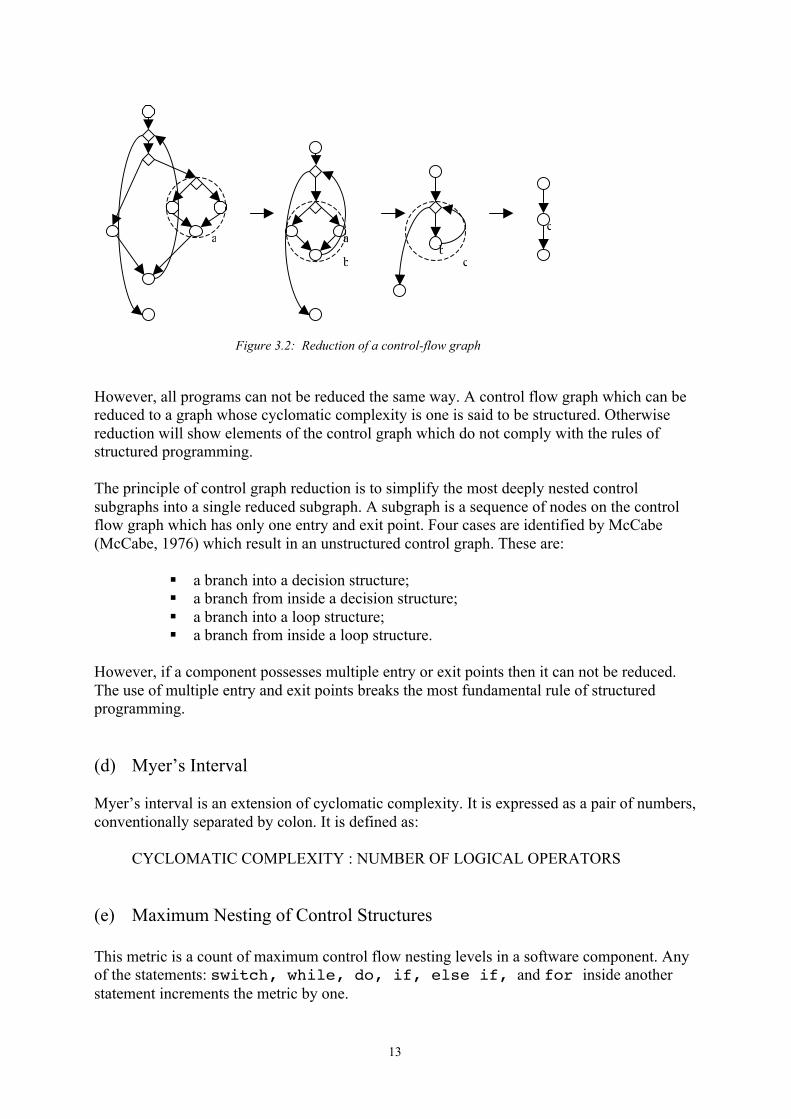
The essential cyclomatic complexity is calculated the same way as the cyclomatic complexity,but is based on a ‘reduced’ control flow graph.
Figure 3.2 shows a control flow graph which can be reduced to a single statement. It meansthat the corresponding program sequence for the control-flow graph can be reduced to aprogram of unit complexity.
13
However, all programs can not be reduced the same way. A control flow graph which can bereduced to a graph whose cyclomatic complexity is one is said to be structured. Otherwisereduction will show elements of the control graph which do not comply with the rules ofstructured programming.
The principle of control graph reduction is to simplify the most deeply nested controlsubgraphs into a single reduced subgraph. A subgraph is a sequence of nodes on the controlflow graph which has only one entry and exit point. Four cases are identified by McCabe(McCabe, 1976) which result in an unstructured control graph. These are:
ß a branch into a decision structure;ß a branch from inside a decision structure;ß a branch into a loop structure;ß a branch from inside a loop structure.
However, if a component possesses multiple entry or exit points then it can not be reduced.The use of multiple entry and exit points breaks the most fundamental rule of structuredprogramming.
(d) Myer’s Interval
Myer’s interval is an extension of cyclomatic complexity. It is expressed as a pair of numbers,conventionally separated by colon. It is defined as:
CYCLOMATIC COMPLEXITY : NUMBER OF LOGICAL OPERATORS
(e) Maximum Nesting of Control Structures
This metric is a count of maximum control flow nesting levels in a software component. Anyof the statements: switch, while, do, if, else if, and for inside anotherstatement increments the metric by one.
aa
bb
c
c
Figure 3.2: Reduction of a control-flow graph

14
(f) Estimated Static Path Count
Estimated static path count is the maximum number of possible paths in the control flow of afunction. It is the number of non-cyclic execution paths in a function. For a thoroughexplanation of the metric see (Nejmeh, 1988).
3.3 Structural Complexity
There exist a great number of metrics that measure different aspects of structural complexity.They are also sometimes referred to as inter-modular metrics, design metrics, or systemmetrics because they express different types of relationships between modules in the systemand can often be calculated already during the design-phase of a project.
There are different ways to present the relationships between the modules in form of a graph.Figure 3.3 shows one of the most common graphs, the P-graph, which shows the callingstructure in a program.
Figure 3.3: Calling structure of a program
Square boxes represent the procedures that can call one another and curved boxes are databases which may be accessed by one or more procedures.
Next follows a summery of some of the interesting structural metrics, with a short descriptionof how they are calculated, and what they measure.
Structural metrics that are mentioned are:
(a) Number of Nodes;(b) Number of Edges;(c) Depth of calling;(d) Number of Function Calls

15
(e) Ince’s Tree Impurity Metric;(f) Yin-Winchester Metric;(g) Henry-Kafura Information Flow Metric;(h) Sheppard Complexity (IF4);(i) Card and Agresti metric;(j) Chapin’s Q metric.
For calculation of some of these metrics a function n(n) is used. It represents the length of theshortest path between the root node and node n in some graph G.
(a) Number of Nodes
As the name applies it is the number of modules (nodes in the system). It is a measure of sizeof the system. In programming language C it can also be used to express a size of anindividual file in terms of the number of functions that it contains.
(b) Number of Edges
As the name says it is the number of edges in the call graph. It expresses the number ofconnections between the modules, and can be used as a measure of coupling (see 3.3.1.1).
(c) Depth of calling
This is a measure of the longest non-recursive chain of calls possible.
Depth of calling = max{n(n), Gn Π}
(d) Ince’s Tree Impurity Metric
This metric is proposed by (Ince & Hekmatpour, 1988) and measures how much a graphdeviates from a tree structure. The more edges added to a tree with a given number of nodes,the higher the value. According to this definition all trees should have the minimum impurity.
Tree impurity = ÂŒGn
(Id(n))^2
where Id is the in-degree of the node. Figure 3.4 shows a two level tree-graph. A callingstructure graph where all modules have in-degree one is said to have a tree structure.

16
Figure 3.4: A two level tree graph
(e) Yin-Winchester Metric
This metric captures the graph impurity of the calling structure. It uses the concept of a level.Nodes on level y are all those with n(x) = y. Yin and Winchester then define two base metricsin terms of which all others can be described. These are Ni and Ai.
Ni = n{ Gx Œ : (x) ≤ i}
Ai = £ix
xOd)(
)(r
where Od(x) is the out-degree of the module x. Ni is the number of nodes and Ai is the numberof edges in the sub-graph which exist on all levels 0 to i.
These metrics are then combined to create three composite metrics namely Ci, Ri, and Di. Themetric Ci measures the number of edges by which the sub-graph (level 0 to i) deviates from atree. If that number of edges were removed and the graph remained connected, then it wouldbe a tree. The Ri metric provides an index of tree impurity for the sub-graph up to level i. Di issimilar except that it considers the graph between levels i – 1 and i. The metrics are definedas:
Ci = Ai - Ni +1
Ri = Ai
1 - Ni1-
Di = 1- 1-i
1-i
A - Ai
N - Ni
(f) Henry-Kafura Information Flow Metric
Henry-Kafuras metric is an approach to measuring the total level of information flow betweenindividual modules and the rest of the system (Henry and Kafura, 1981). A local flow exists ifeither:
1. a module invokes a second module and passes information to it; or2. the invoked module returns a result to the caller.

17
Similarly, a local indirect flow exists if the invoked module returns information that issubsequently passed to a second invoked module. A global flow exists if information flowsfrom one module to another via a global structure.
With these notions two particular attributes of information can be described. The fan-in of amodule M is the number of local flows that terminate at M, plus the number of data structuresfrom which the information is retrieved by M. Similarly the fan-out of a module M is thenumber of local flows that emanate from M, plus the number of data structures that areupdated by M.
Based on these concepts Henry-Kafura Information Flow Metric is defined as:
Information flow complexity = length(M)*(fan-in(M)*fan-out(M))2
where length(M) is some measure of the modules size, e.g. the number of statements.
(g) Sheppard Complexity (IF4)
Sheppards complexity metric is just a modification of Henry-Kafura Information Flow Metric(Sheppard and Ince, 1990):
Sheppard complexity(M) = (fan-in(M)*fan-out(M))2
(h) Card and Agresti metric
Card and Agresti metric, sometimes also referred to as system complexity (Card & Agresti,1988) is a composite measure of complexity inside procedures and between them. It measuresthe complexity of a system design in terms of procedure calls, parameter passing and data use.
System complexity consists of two elements:
• SC Structural complexity, which measures the external complexity of a procedure, thatis, the calls between procedures.
• DC Data complexity, also known as the local or internal complexity of a procedure.
The following definitions are used:
Fan-out = Structural fan-out = Number of other procedures this procedure calls
v = number of input/output variables for a procedure
Structural complexity SC for a procedure equals its fan-out squared. A procedure that calls alarge number of other procedures has a relatively high structural complexity.
SC = fan-out2
Data complexity DC for a procedure is defined by the following equation:
DC = v / (fan-out + 1)
With these two functions one can calculate the complexity of the entire system:

18
Total system complexity SYSC = sum(SC + DC) over all proceduresRelative system complexity RSYSC = average(SC + DC) over all procedures
The relative system complexity measures the average complexity of procedures. It is anormalized measure for the entire system and it does not depend on the system size. It thusallows for design complexity evaluation among different systems.
(i) Chapin’s Q metricQ-metric is quite similar to the card and agresti metric. Chapin does not only identify theinputs and outputs to each module. He also assigns a weighting factor depending on thepurpose of the data since it influences the complexity of the module interface. The followingtypes of data are recognised:
‘P’ data–inputs required for processing;‘M’ data–inputs that are modified by the execution of the module;‘C’ data–inputs that control decisions or selections;‘T’ data–through data that is transmitted unchanged.
A weighting factor is assigned to each type to indicate the complexity of the control structureto invoke the module.
3.3.1 System Design
The goal with imposing the max/min-boundaries for modules on structural complexity metricsis to gain a program that is as well structured as possible.
Below, in the following sub-chapter, two notions, coupling and cohesion, that are used toevaluate the quality of the program design, are presented. After that follows a brief summeryand a description of the design errors that can occur and that we can avoid by having “well”structured programs.
3.3.1.1 Coupling and Cohesion
These two notions of design structure (coupling and cohesion) are the ones that are most oftenused to evaluate the design quality, or in the later stages, the quality of the system structure.A thorough explanation of these notions can be found in the book software metrics (Fenton &Pfleeger, 1997).
Coupling is the degree of interdependence between modules (Yourdon & Constantine, 1979).Usually coupling expresses interdependence between two modules, rather than between allmodules in the system. Global coupling is the measure of coupling for the whole system andcan be derived from the coupling among the possible pairs.
There are several well established relations involving coupling, that suggests at least anordinal scale of measurement. Given modules x and y, we can create a classification forcoupling, defining six relations on the set of pairs of modules:

19
ß No coupling relation R0: x and y have no communication: they are totallyindependent of one another.
ß Data coupling relation R1: x and y communicate by parameters, where eachparameter is either a single data element or homogeneous set of data items thatincorporate no control element. This type of coupling is necessary for anycommunication between modules.
ß Stamp coupling relation R2: x and y accept the same record type as a parameter.This type of coupling may cause interdependency between otherwise unrelatedmodules.
ß Control coupling relation R3: x passes a parameter to y with the intention ofcontrolling its behaviour; that is, the parameter is a flag.
ß Common coupling relation R4: x and y refer to the same global data. This type ofcoupling is undesirable; if the format of the global data must be changed, then allcommon-coupled modules must also be changed
ß Content coupling relation R5: x refers to the inside of y; that is, it branches into,changes data in, or alters a statement in y.
The relations are listed from the least dependent at the top to most dependent at the bottom, sothat Ri > Rj for i > j. X and y are considered loosely coupled when i is 1 or 2, and tightlycoupled when i is 4 or 5.
The cohesion of the module is the extent to which its individual components are needed toperform the same task. As with coupling there are no standard measures of cohesion. Yourdonand Constantine proposed classes of cohesion that provide an ordinal scale of measurement(Yourdon and Constantine, 1979):
ß Functional: the module performs a single well-defined function.ß Sequential: the module performs more than one function, but they occur in an order
prescribed by the specification.ß Communicational: the module performs multiple functions, but all on the same
body of data (which is not organised as a single type of structure).ß Procedural: the module performs more than one function, and they are related only
to a general procedure affected by the software.ß Temporal: the module performs more than one function, and they are related only
by the fact that they must occur within the same timespan.ß Logical: the module performs more than one function, and they are related only
logically.ß Coincidental: the module performs more than one function, and they are unrelated.
These categories of cohesion are listed from most desirable (functional) to least desirable.
There is no obvious measurement procedure for determining the level of cohesion in a givenmodule. However, we can get a rough idea by writing down a sentence to describe themodule’s purpose. A good designer should have already done so, but a module with highcohesion is unlikely to have been produced by a good designer! If it is impossible to describeits purpose in a single sentence, then the module is likely to have coincidental cohesion. If thesentence contains words such as “initialize”, then the module is likely to have temporalcohesion. Suppose the sentence contains a verb not followed by a specific object, such as

20
“generate output”, or “edit files”, then the module probably has logical cohesion. When thedescriptive sentence contains words relating to time (such as “first”, “then”, “after”), then themodule is likely to have sequential cohesion. Finally, if the sentence is compound or containsmore than one verb, then the module is almost certainly performing more than one functionand so is likely to have sequential or communicational cohesion.
According to classic approach the designer should seek an appropriate balance between lowcoupling and high cohesion; that is, high cohesion (preferably functional) and lowcoupling (preferably no coupling–or data or stamp coupling) are desirable.
According to more recent trends the most desirable type of cohesion is abstract cohesion,which means abstract data type encapsulation as modules. By encapsulating an abstract datatype as a module, we characterise it in terms of the operations it may perform on certainobjects. Such a module may perform several different functions, but they are all related in thesense that they characterise the abstract data type precisely. For example, a moduleencapsulating the abstract data type “stack” should perform precisely those functions weassociate with a stack of objects, namely: create, is empty, pop, push, and so on.
3.3.1.2 Design Errors
Coupling and cohesion are the consequences, or symptoms of design errors. They are noterrors in themselves. This is significant because it means that they indicate underlyingproblems with a design but do not directly suggest a solution. By striving for the design that isas “good” as possible, meaning that cohesion between modules is as high and coupling as lowas possible, these errors can be avoided.
Also the structural complexity metrics (suggested in section 3.3), can not directly point outdesign errors. However, they too can be used to suggest where the errors might have occurred.By verifying parts of the system where modules with too high values of structural metrics aresituated, some of the design errors can be identified and corrected. That can be done either bychanging the modules or redesigning that part of the system. Also by making sure that themodules in the system comply to the recommended max/min-values for the system metrics,some of the design errors can be avoided.
Sheppard and Ince (Sheppard and Ince, 1990), continuing on the work of Stevens et al.(Stevens et al., 1978), suggested an eightfold classification of structural design errors. Brieflythese are:
(a) missing levels of functional abstraction;(b) multiple functionality;(c) split functionality;(d) misplaced functions;(e) duplicate functionality;(f) inadequate data object isolation;(g) duplicate data objects;(h) over-loaded data objects.
21
The first five classes are essentially shortcomings in the functional design, whilst theremaining three classes are errors of data design.
(a) Missing levels of functional abstraction
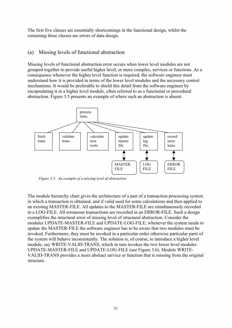
Missing levels of functional abstraction error occurs when lower level modules are notgrouped together to provide useful higher level, or more complex, services or functions. As aconsequence whenever the higher level function is required, the software engineer mustunderstand how it is provided in terms of the lower level modules and the necessary controlmechanisms. It would be preferable to shield this detail from the software engineer byencapsulating it in a higher level module, often referred to as a functional or proceduralabstraction. Figure 3.5 presents an example of where such an abstraction is absent.
Figure 3.5: An example of a missing level of abstraction
The module hierarchy chart gives the architecture of a part of a transaction processing systemin which a transaction is obtained, and if valid used for some calculations and then applied toan existing MASTER-FILE. All updates to the MASTER-FILE are simultaneously recordedin a LOG-FILE. All erroneous transactions are recorded in an ERROR-FILE. Such a designexemplifies the structural error of missing level of structural abstraction. Consider themodules UPDATE-MASTER-FILE and UPDATE-LOG-FILE; whenever the system needs toupdate the MASTER-FILE the software engineer has to be aware that two modules must beinvoked. Furthermore, they must be invoked in a particular order otherwise particular parts ofthe system will behave inconsistently. The solution is, of course, to introduce a higher levelmodule, say WRITE-VALID-TRANS, which in turn invokes the two lower level modulesUPDATE-MASTER-FILE and UPDATE-LOG-FILE (see Figure 3.6). Module WRITE-VALID-TRANS provides a more abstract service or function that is missing from the originalstructure.
processtrans.
fetchtrans.
validatetrans.
calculatenewtools
updatemasterfile
updatelogfile
recorderrortrans.
MASTERFILE
LOGFILE
ERRORFILE

22
Figure 3.6: Introduction of missing abstraction
The empirical study performed by Sheppard and Ince (Sheppard & Ince, 1990) shows that thistype of error is rather commonplace. This is disturbing because these structures maypotentially cause a number of problems:
ß First, they hinder the re-use of higher level services in a software system;
ß Second, they are maintenance “time bombs”. Suppose the system is modified atsome subsequent stage and an additional transaction update of the MASTER-FILEis required, the maintainer has the added burden of having to remember to alsoupdate the LOG-FILE and in the correct order. Such oversights can lead to costlysystem failures;
ß Third, they make the system harder to understand since they place the task ofinferring the service provided by groups of lower level modules upon the softwareengineer.
The classic symptoms of this design error are either a module with an unusually large numberof subordinates; in this case the module PROCESS-TRANS has six subordinate modules; or anumber of modules that all invoke the same set of subordinates implying that this subordinateset represents some useful function.
(b) Multiple functionality
This class of structural design error indicates, as the name suggests, that a module implementsmore than one function. This is related to the concept of low module cohesion (see chapter3.3.1.1), where the various parts of the module are unrelated in terms of a service or functionsthat they provide. Figure 3.7 shows the architecture of part of a menu driven system to controluser-ids which allow access to some computer system, including options to add, remove, andlist user-ids.
writevalidtrans.
updatemaster file
updatelog file
MASTERFILE
LOGFILE

23
Figure 3.7: Multiple functionality
At a first glance this appears a very plausible design, but unfortunately the modulePROCESS-MENU contains a number of functions including: displaying a menu, obtaining aresponse, validating the response, displaying an error message if appropriate and thenselecting the required menu facility. Does this matter? The answer is an emphatic yes–as thedesign stands PROCESS-MENU is harder to understand due to the interleaving of severalfunctions within a single module. Furthermore reuse of these functions is almost impossible.And the corollary of such a strategy is the duplication of functions through the system, such asdisplaying the menus and fetching responses, with the consequent maintenance “time bombs”.
These errors may be indicated by a potentially large number of information flows into and outof a module. An exception is library routines, which have a high number of informationflows. They should always occur at the lowest calling level.
(c) Split functionality
This type of error is in many ways the antithesis of multiple functionality as it involves asingle function being distributed among several modules. Figure 3.8 provides an example ofsplit functionality where the functional requirement to validate a part number is distributedover three modules in a highly arbitrary fashion.
Figure 3.8: Split functionality examples
The only symptoms manifested on a module hierarchy chart are possible increases in levels ofcoupling of information flow between the modules concerned.
PROCESSMENU
adduser-id
removeuser-id
listuser-id
validatepart-no
part-nook?
checkpart-no

24
(d) Misplaced functions
Misplaced functions are a class of structural errors where functionally related modules areplaced unnecessarily far apart by the system architecture leading to a proliferation ofinformation flows, parameters and modules that have little purpose other than to routeinformation. Such an example is given by the Figure 3.9 where the module HANDLE-COMMAND-ERROR is misplaced since it is closely related to the module VALIDATE-COMMAND. Clearly the solution would be to move the module to become a subordinate ofthe module VALIDATE-COMMAND.
Figure 3.9: Misplaced function example
The consequences of misplaced functions are threefold:
ß First, these types of structures severely inhibit the possibilities of function reuse;ß Second, this provides great scope for unwanted “side effects” if maintenance
changes occur;ß Third, such structures present considerable barriers to comprehension.
Possible symptoms are additional information flows to and from the misplaced modules.
(e) Duplicate functionality
Duplicated functions are normally disguised, frequently by the use of synonyms for modulenames (e.g. FETCH-COMMAND and GET-COMMAND). Where duplicate functionalityoccurs in combination with other structural problems such as multiple functionality it may beeven harder to isolate as the module name may reflect another function which it satisfies.Potential maintenance problems are the main issue with this type of error.
Unfortunately there are few if any symptoms for duplicate functionality in a module, so it isvery difficult to detect with structural metrics.
(f) Inadequate data object isolation
This is the first of three structural error categories that concerns data objects, although thedefinition of data object should be generalised to include devices. Unfortunately none of thestructural metrics suggested in section 3.3 are concerned with data models, so they are notcapable of detecting these classes of errors.
processcommand
Fetchcommand
HandleCommanderror
processvalidcommand
getcommand
validatecommand
error
error
error

25
Avoiding inadequate data object isolation errors has been one of the prime motivations behindthe objected-oriented approaches (Booch, 1986), yet despite being a relatively widelyunderstood principle our empirical analysis would suggest is not well adhered to.Maintenance activities may be one of the reasons for a breakdown of data object isolation.The other explanations are poor communication within a development project and multiplefunctionality so that data object access routines are packed with other functions, inhibitingreuse.Figure 3.10 illustrates a partial system architecture where many modules all access the samedata object, ACTIVITIES-TABLE.
Figure 3.10: Lack of data object isolation
A better solution is to restrict access to ACTIVITIES-TABLE to the minimal set of primitivefunctions, possibly ADD, DELETE and FETCH and use these as building blocks to constructthe more complex operations.
As the architecture stands it may lead to a number of problems:
ß First, since the structure of ACTIVITIES-TABLE may be complex this will makethe software harder to comprehend and with an increase in the probability ofcommitting errors as the processing details for manipulating the object cannot beseparated from the remainder of a module’s functionality;
ß Second, introducing the data integrity checks will prove to be difficult and result inmuch duplication of functionality. The usual consequence of this type of systemstructure is to treat it as a powerful disincentive to build in any such integrityfeatures;
ß Third, sharing the data object in this fashion effectively couples many modulestogether with a resultant increase in the probability of side effects.
Symptoms for this class of errors are a high level of access to a data object which may beobserved from a module hierarchy diagram, or suggested by some structure metrics. Thiserror is a particular case of multiple functionality for a set of modules that all share a givendata object. Inadequate data object isolation errors are very common, and are given specialemphasis in the literature (see for example (Parnas, 1972), (Parnas, 1979) or (Stevens, 1978)).
addactivity
updateactivity
listactivities
checkactivity
linkactivities
ACTIVITYTABLE

26
(g) Duplicate data objects
The duplication of parts or all of the data objects is seldom considered to be an issue bysoftware engineers, however, it may have considerable impact upon a design andconsequently upon a range of quality factors of the resultant implementation. Synonyms oftendisguise duplication, particularly if the system has had a long maintenance history. Apart fromthe possibilities of data inconsistency, duplicate data objects lead to unnecessarily complexsoftware and a loss of maintainability.This is a rather uncommon error, and most often it is left for the database worker to make sureit does not occur. However software engineers ought at least to be aware that such errors existand try to prevent them from happening.
(h) Over-loaded data objects
Our final class of structural design errors derive from over-loaded data objects. Such dataobjects are used by more than one module and assigned more than one meaning. In theexample given in Figure 3.11, the two unrelated modules CHECK-INPUT and DISPLAY-MESSAGE both share the same data object FLAG although they use it for different purposes.In other words FLAG is over-loaded with two meanings. This is an undesirable state of affairsas it allows for potentially disastrous side effects, and makes the system harder to understandand maintain.
Figure 3.11: Over-loaded data object
This over-loading of data objects cannot be detected without knowledge of the meaning ofdata. It is the mapping from the conceptual data model to its physical realisation that indicatesthe presence of this class of errors.
3.4 Combined Metrics
Combined metrics are metrics that try to measure more than one aspect of complexity.
Some of the earlier mentioned metrics are also combined, but since they are mentioned astext, component or structure metrics in the literature I also refer to them as such. For exampleHenry-Kafura metric (see chapter 3.4) tries to give a measure of both length and structuralcomplexity.
checkinput
displaymessage
FLAG

27
The goal with combined metrics is to more accurately point out the most complex modules inthe system, giving a better approximation of modules overall complexity. The problem withthem is that they do not specifically indicate in what way a module is complex, or how itshould be redesigned.
An example of a combined metric is Akiyama’s Criterion. It is the sum of the cyclomaticcomplexity (CYC) and the number of function calls (SUB).
AKI = CYC + SUB
A thorough description of the metric is given in (Akiyama, 1971) and (Schooman, 1983).

28
4 EMPIRICAL INVESTIGATION
An empirical investigation can be used to evaluate a technique, a method or a tool. What isinteresting for this thesis is that empirical investigation can be used to evaluate which of thecomplexity metrics that are correlated with software quality, or which metric is most highlycorrelated with software quality.
The book Software Metrics (Fenton & Pfleeger, 1997), describes different types of empiricalinvestigations in detail.
There are three types of empirical investigations: survey, case study and formal experiment.
Before performing any kind of empirical investigation you have to decide what it is you wantto investigate and express it as a hypothesis you want to test. That is, you must specify whatit is you want to know. For example your hypothesis may be “Number of bugs in a module isdependent on the module’s size”.
There are a couple of factors that you have to consider in choosing which empiricalinvestigation to conduct. The first step is to decide whether investigation is retrospective ornot. If, that what you want to investigate has already occurred, then a survey or a case studycan be performed. If it has not yet occurred, than the choice is between a case study and aformal experiment. Another important factor is the level of control needed to perform aformal experiment. Only if you have a very high level of control over the variables that canaffect the outcome, can you consider an experiment. Also the degree to which you canreplicate the experiment is important. If replication is not possible, or is too costly, then aformal experiment cannot be done.
The relationships can be suggested by a case study or a survey, but to clearly understand andverify some relationships a formal experiment must be conducted. Usually the suggestionsgained by a case study are “given more weight” then those gained by a survey. That is, theyare considered to be stronger suggestions.
In the next three sections different types of empirical investigations are briefly described.
4.1 Survey
In general a survey is a study of a situation in retrospective to try to document relationshipsand outcomes. A survey is always done after an event has occurred. Surveys in softwareengineering pull a set of data from an event that occurred, to determine trends or relationships.

29
4.2 Case Study
In a case study one situation is usually compared with another. It can be organised as a sisterproject, baseline, or random selection.
Sister project: Two projects selected, called sister projects are compared to each other. Eachof them is typical for the organisation and has similar values for the state variables that aregoing to be measured.
Baselines: A project is compared to a baseline. Data is gathered from various projects in theorganisation, regardless of how different they are from each other. Then a measure of thecentral tendency and dispersion of the collected data is calculated. That presents an averagesituation, a typical situation in the company, a baseline.
Random selection: A single project is partitioned into parts. Then for example one part usessome new technique and others do not.
4.3 Formal Experiment
In short, a formal experiment is a rigorous, controlled investigation of an activity, where keyfactors are identified and manipulated to see the effect on the outcome.

30
5 TECHNIQUES TO DETERMINE MAX, MIN AND UPPERLIMIT VALUES
This chapter describes Demographic Analysis. It is a statistical technique that was used byLes Hatton (Hatton, 1995), to determine suitable max-values for cyclomatic complexity,estimated static path count and some other complexity metrics.
The following subchapter describes how demographic analysis can be used to determinesuitable max-value for some complexity metric. Using two-percentile instead of ten-percentile, the same technique can be used to determine a suitable upper limit value.
Unfortunately no statistical technique, that would enable me to determine min-values forcomplexity metrics, came to my knowledge.
5.1 Demographic Analysis
Demographic analysis was a statistical technique that I used to determine suitable max andupper limit boundaries for chosen complexity measures for a number of program packages.
Initially, I did not have information about any kind of internal knowledge about problematicfunctions or files, little less about statistics over occurred faults, failures or changes in thesesoftware packages. Demographic analysis seemed to be the only way to evaluate thesesoftware packages and come to some kind of conclusion about suitable max-boundaries forchosen metrics.
Demographic analysis can also be used to monitor the progress in limiting the complexitieswhen complexity limitation has been put in place.
In essence, the technique goes as follows:
ß The values for certain file–or function complexity metric are determined for all filesor functions in a large population of software (in this case one of the chosensoftware packages). All metrics evaluated are monotonic in the sense that highervalues are associated with poorer software.
ß Then those files or functions are split up into percentile node-points as follows:
[a0, a1] contains the worst 10 per cent of all values[a0, a2] contains the worst 20 per cent of all value..[a0, a10] contains the worst 100 per cent of all values
where ai is the appropriate value of the metric (Hatton, 1995).

31
Figures 5.1 and 5.2 show how this analysis was performed for Cyclomatic Complexity andMaximum nesting of control structures in package II.
If we look at the figures, the diagram to the right shows a graph that displays the results of theanalysis of software package II for certain complexity metric, performed by softwaredevelopment tool QA C. Each point in the graph represents a function, with its coordinate onthe horisontal axis showing the number of the function and coordinate on the vertical axisshowing functions complexity.
Each marked point in the graph represents the function with highest complexity value incertain percentile group. The table on the left shows complexity values for each of the markedpoints.
Figure 5.1 The distribution of Cyclomatic Complexity for the whole population in software package II
Percentilevalue
CyclomaticComplexity
0 89
5 18
10 8
20 5
30 3
40 2
50 2
60 1
70 1
80 1
90 1
100 1
functions
com
plex
ity

32
Figure 5.2 The distribution of Maximum nesting of control structures for the whole population in softwarepackage II
These results are used to determine suitable max-values for chosen complexities in theevaluated software package. Experience has shown that in a software package where nocomplexity limiting was in operation, the 10% of functions (or files, depending on whetherfunction or file metric was evaluated) takes on the lion’s share of the resources and isresponsible for most of the errors (Hatton, 1995). That is why ten percentile is a good value tobe used as max-value for the metric in the evaluated program package.
Percentilevalue
Maximumnesting ofcontrolstructures
0 325 5
10* 420 230 140 150 160 070 080 090 0
100 0
*ten percentile
functions
com
plex
ity

33
6 EVALUATION OF COMPLEXITY METRICS
I concentrated my experimental evaluation on complexity metrics that the softwaredevelopment tool QA C can calculate. There were three reasons for that:
ß QA C is used by many software developers at Scania;ß QA C can calculate almost all of the most common complexity metrics;ß I did not have enough time to do this kind of investigation for other complexity
metrics. To do that I would have to evaluate other software development tools, findout which one can calculate metrics that I’m interested in, learn how to use it, andthen to do the evaluation. It would also probably be impossible, due to the fact thatScania would then have to purchase another software development tool just for myevaluation, which is too weak a motivation.
QA C can calculate a great number of software metrics, most of which are complexitymetrics. QA C divides them into two groups: file metrics and function metrics.The difference between these two groups is in the module for which they measure thecomplexity. Function metrics measure the complexity of a function-module and file metrics ofa file-module. E.g. number of executable lines measures the size of a function, while Numberof statements measures size of a file. Since a file is composed of a number of functions thesemodules are dependent on each other, and so are the file and function complexity metrics.
In this chapter I present three ways in which I tried to evaluate which of the complexitymetrics that are correlated with the quality of real time software.
In chapter 6.1 my initial evaluation is presented. I relied solely on the experience of otherpeople and on the results of case studies performed on similar kind of safety related real timebased software. From these literature studies I came to conclusions on which complexitymetrics that could be correlated with the quality of software produced here.
Chapter 6.2 presents the survey investigation. The goal was to find out if there was any kindof knowledge about problematic (fault/failure prone), functions or files in different softwarepackages, or some other knowledge about faults or failures. The investigation led to a coupleof interesting results. Amongst others a number of problematic functions and files wererecognised. They were later used to suggest which complexity metrics could be correlatedwith software quality.
Chapter 6.3 presents case study performed on package III, for which there existed adocumented history about changes. Based on that history, a case study was performed tosuggest which of the complexity metrics could be correlated with the software quality.
These three chapters are presented in order of the “strength of their suggestion”. That meansthat conclusions gained from survey investigation give stronger suggestion, than those gainedby literature study. Also conclusions gained by case study give stronger suggestion than thosegained by the survey.
34
Chapter 6.4 looks at the conclusions from all investigations to suggest which of thecomplexity metrics that are correlated with software quality. In chapter 7, suitable max, minand upper limit values are then calculated for these metrics.
6.1 Using the Experience of Others
During my literature studies I found four complexity metrics, which QA C can calculate, to bethe most interesting. They were mentioned as being correlated with the software quality inmost of the cases I found. These complexity metrics are:
ß Cyclomatic complexityß Maximum nesting of control structuresß Estimated static path countß Number of function calls
I contacted one of the experts in the field, Les Hatton, the author of the book Safer C (Hatton,1995), and in his personal opinion only estimated static path count–and cyclomaticcomplexity metrics were always correlated with quality of the software.
Size of the modules also seemed to be an important aspect of software complexity, as thereexist many case studies proving its correlation with the software quality. I, however, decidedto wait, because there were several (see chapter 3.1) and I wanted to learn more about thembefore choosing one to evaluate. At the end I decided on Number of executable lines since:
ß It appeared that all of the size complexity metrics are correlated with the softwarequality pretty much equally. When, e.g., changing a module so that it leads to adecrease or increase of one of the size metrics, other size metrics also increase ordecrease with relatively the same amount. That is why it didn’t really matter whichone I chose, since they all pretty much equally successfully limited the sizecomplexity.
ß QA C measures the size of the functions only in number of executable lines of codeand in number of maintainable code lines. Since the difference between the two isthat Number of maintainable code lines apart from the executable lines also countsall lines of code including blank and comment lines which do not influence thecomplexity, I chose to evaluate the Number of executable lines.
These five metrics were also chosen because they together limit all three aspects of softwarecomplexity. Number of executable lines limits the text complexity; Cyclomatic complexity,maximum nesting of control structures and estimated static path count limit the componentcomplexity; and number of function calls limits the system complexity.
All of the mentioned metrics are function metrics in QA C. Regarding QA C file metrics, Icould not find case studies for any of them except for Halstead’s metrics. I also was not sureof their correlation with software quality, so I decided to do more research before drawing anyconclusions.

35
6.2 Survey Investigation
In order to gain the information that could suggest which of the complexity metrics that arecorrelated with software quality, I performed a survey. I tried to answer the following twoquestions for each software package:
1. Which of the functions and files in the package were the most problematic andfault/failure-prone?
2. What was the time ratio between the three components of maintenance: corrective(correction of failures detected), adaptive (prevention of failures) and improvement(adding new features)?
The survey led to couple of interesting results:
ß 21 of the most problematic and fault/failure-prone functions, and 10 files from four ofthe packages were identified.
ß I found out that there existed a somewhat well documented history on changes andbugs for at least one of the packages.
ß Most, around 2/3, of the maintenance time went on improvement.
The first result was used to suggest which of the complexity metrics that could be correlatedwith software quality–which was the original goal of the survey.
The second result was used to perform a case study on package III and show with greatercertainty which of the complexity metrics that could be correlated with software quality (seechapter 6.3). Also suitable max-values for the complexity metrics were calculated.
The third result showed that the improvement was the most substantial part of the softwaremaintenance. That in turn, proved the importance of having well structured and easyunderstandable modules as well as good design of the system.
6.2.1 Investigation of Problematic Functions
The results of the investigation of problematic functions with QA C can be seen in appendixC. As can be seen in the appendix, QA C does not just calculate the complexity metrics forthe functions, but a number of other software metrics as well.
From the tables in the appendix C, table 6.1 is extracted. It shows software metrics averagesfor the program packages, problematic functions and the average for all of the functions. Thetable shows only the complexity metrics.
The two bottom rows show ratios PF/ALL and PF/AP. PF/ALL is the ratio between theaverage (of some complexity metric) for the problematic functions and the average for all ofthe functions and PF/AP between the average for the problematic functions and the averagefor the software packages.

36
The assumption is that the bigger the ratio, the better the correlation between the metric andthe software quality. However it is only a weak suggestion. To prove that one metric is morecorrelated with software quality than some other, an experiment must be conducted.
As can be seen in the table, metrics are divided into groups according to the type of thecomplexity that they are measuring.
Summary of the conclusions from the table 6.1 is following:
ß All the metrics suggested in chapter 6.1, gave the indication of being correlated withsoftware quality.
ß Maximum nesting of control structures gave the indication of being less correlatedwith the software quality then the other four metrics.
ß Other complexity metrics that QA C can calculate, were suggested as beingcorrelated with the software quality. They are: the Number of local variablesdeclared, Myer’s interval and Essential cyclomatic complexity.
ß Myers interval was especially interesting since it had more than twice as highPF/ALL-ratio than cyclomatic complexity and second highest ratio of all metrics.Since Myers interval is a sum of cyclomatic complexity and a number of logicaloperators, this suggest that it could be viewed on as an improvement of cyclomaticcomplexity.
There are some metrics from the table that were not mentioned in the last conclusion thoughthey had high PF/ALL–or PF/AP-ratios. Reason for that is that they are deduced from someother metrics. When limiting these other metrics they are limited as well.

37
List of the function software metrics:
STAKI Akiyama's Criterion. STLCT Number of local variables declared STPBG Path-based residual bug estimateSTBAK Number of backward jumps STLIN Number of maintainable code lines STPDN Path DensitySTCYC Cyclomatic Complexity STLOP Number of logical operators STPTH Estimated static path countSTELF Number of dangling else-if.s STM07 Essential Cyclomatic Complexity STSUB Number of function callsSTGTO Number of goto.s STM19 Number of Exit Points STUNV Number of unused and unreused variablesSTKDN Knot density STMCC Myer.s Interval STXLN Number of executable linesSTKNT Knot count STMIF Maximum nesting of control structures
Table 6.1: Complexity metrics averages for the program packages & problematic functions, divided into complexity groups
Text Complexity Component ComplexitySystemComplexity
S & CComplexity
T & CComplexity
PACKAGES STLCT STLIN STXLN STCYC STM07 STMCC STMIF STPBG STPTH STSUB STAKI STPDNPackage I 3,1 62,0 23,7 5,6 1,0 4,3 2,0 0,6 591291,9 4,9 10,5 2071,4Package II 0,7 20,2 12,0 3,6 1,1 0,4 0,9 0,4 93,2 2,0 5,7 1,8Package III 1,3 28,3 16,4 4,8 1,2 1,2 1,1 0,4 516296,3 5,7 10,5 1839,3Package IV 1,0 24,8 14,9 4,4 1,2 0,9 1,3 0,5 2294641,9 4,9 9,3 12797,9Package V 1,3 68,0 33,8 8,9 1,5 2,5 2,1 1,1 6082222,5 5,5 14,4 34802,1Package VI 0,7 35,9 18,8 4,4 1,2 1,7 1,2 0,6 4971468,6 2,6 7,0 15282,6Package VII 1,7 29,3 14,2 3,1 1,0 0,9 0,9 0,4 1353378,9 2,2 5,3 4571,2AVERAGEPACKAGES 1,4 38,4 19,1 5,0 1,2 1,7 1,4 0,6 2258484,8 4,0 9,0 10195,2ALL 1,3 31,4 16,1 4,0 1,1 1,2 1,1 0,5 2047352,2 3,1 7,1 7754,9ProblematicFunctions 14,4 401,3 233,4 49,4 10,7 35,4 7,5 5,3 106874481,5 35,2 84,7 290862,4PF/ALL 11,2 12,8 14,5 12,2 9,6 29,6 6,8 11,4 52,2 11,4 11,9 37,5PF/AP 10,3 10,5 12,2 9,9 9,1 20,8 5,5 9,3 47,3 8,9 9,5 28,5

38
6.2.2 Investigation of Problematic Files
Results of the investigation on the problematic files are given in the second part of theappendix D. It was performed the same way as the investigation of problematic functions.
Data gained for the problematic files proved to be useless. I could not use it to come to anyconclusions about file complexity metrics. There are a couple of reasons for that:
1. PF/ALL–and PF/AP ratios are too small to come up with any conclusionsabout the metrics, given the insecurity in the investigation.
2. The metric that measures the number of non-header comments had thehighest PF/ALL–and PF/AP ratios of all text complexity metrics. In theoryit should be least connected to the software quality.
3. Most of the suggested files were weakly suggested to be problematic. Indifference all the functions were directly recognised as problematic, whilefiles were recommended on very weak basis.
6.3 Case Study
During the survey I studied the documented history about bug related changes, in one of theprogram packages. Based on that history a case study was performed.
For each file and function, the bugs that occurred in them were counted. Table 6.2 shows howmany functions had a certain number of bugs, and table 6.3 show the same thing for files inpackage III.
Table 6.2: Shows the number of functions havinga certain number of bugs
Number of Bugs Number of Functions0 1581 172 63 1
Table 6.3: Shows the number of files havinga certain number of bugs
Number of Bugs Number of Files0 91 12 43 34 05 16 07 1

39
As can be seen from the tables, the number of bugs in files is different from the number ofbugs in functions. The reason for that is that a bug which occurred in one file could be tracedto two or more functions.
6.3.1 Investigation of Correlation between Bugs and Complexity Metrics
To find out which of the complexity metrics are correlated with the number of bugs in thefunctions and files I calculated a correlation coefficient for each metric.
Correlation coefficient is used to determine the relationship between two properties. In thiscase it is the relationship between one of the complexity metrics and the number of bugs.
The correlation coefficient is a number between -1 and 1. If there is no relationship betweenthe predicted values and the actual values the correlation coefficient is 0 or very low (thepredicted values are no better than random numbers). As the strength of the relationshipbetween the predicted values and actual values increases so does the correlation coefficient. A perfect fit gives a coefficient of 1.0. A perfect negative fit gives a coefficient of -1.0. Thusthe higher the correlation coefficient the better. Figure 6.1, taken from the Math World onlinemagazine (Mathworld, 2004), illustrates how the correlation coefficient reflects therelationship between two values.
Figure 6.1: Illustration of the correlation coefficient. Correlation coefficient equals r2.
Results of the calculations of correlation coefficients for the software metrics can be seen inappendix D.
From the appendix D I extract only the file complexity metrics, and present them in the table6.4. Other complexity metrics that can be deduced from some of these extracted metrics arenot taken into table.
Rank represents the size of the correlation coefficient for some complexity metric relative toother correlation coefficients in the table. The higher the rank-number for a complexitymetric, the bigger its correlation coefficient.

40
Table 6.4: Correlation coefficients & ranks for the relevant function metrics
ComplexityType Text Complexity Component ComplexityComplexityMetrics STLCT STLIN STXLN STCYC STM07 STMCC STMIF STPBG STPTHCorrelationCoefficient 0,387 0,551 0,536 0,471 0,254 0,481 0,406 0,458 0,465
Rank 10 3 4 6 11 5 9 8 7
Table 6.4 (the extension): Correlation coefficients & ranks for the relevant function metrics
Complexity Type System Complexity S & C1 Complexity T & C ComplexityComplexity Metrics STSUB STAKI STPDNCorrelation Coefficient 0,640 0,607 0,094Rank 1 2 13
As can be seen in the table, metrics are divided into groups according to the type of thecomplexity that they are measuring.
Results of the calculations of correlation coefficients for the file software metrics can be seenin table 6.5. The same kind of “extraction” was not performed for the file complexity metricsin the table 6.5, since that table contains only complexity metrics. All of the metrics in thetable measure the text complexity of files except for two. They measure system complexityamong the functions in the file, or as also can be seen, files internal component complexity.They are estimated function coupling and number of external variables.
1 S & C equals System & Component

41
List of the file software metrics:
STBME COCOMO Embedded Programmer Months STM20 Number of Operand Occurrences STTDO COCOMO Organic Total MonthsSTBMO COCOMO Organic Programmer Months STM21 Number of Operator Occurrences STTDS COCOMO Semi-Detached Total MonthsSTBMS COCOMO Semi-detached Programmer Months STM22 Number of Statements STTLN Total Preprocessed Source LinesSTBUG Residual Bugs (token-based estimate) STM28 Number of Non-Header Comments STTOT Total Number of TokensSTCDN Comment o Code Ratio STM33 Number of Internal Comments STTPP Total Unpreprocessed Source LinesSTDEV Estimated Development Time STMOB Code Mobility STVAR Number of IdentifiersSTDIF Program Difficulty STOPN Halstead Distinct Operands STVOL Program VolumeSTECT Number of External Variables STOPT Halstead Distinct Operators STZIP Zipf Prediction of STTOTSTEFF Program Effort STPRT Estimated Porting TimeSTFCO Estimated Function Coupling STSCT Number of Static VariablesSTFNC Number of Function Definitions STSHN Shannon Information ContentSTHAL Halstead Prediction Of STTOT STTDE COCOMO Embedded Total Months
Table 6.5: Correlation coefficients & ranks for the file metricsComplexity Metrics STBUG STDIF STECT STEFF STFCO STFNC STHAL STM20 STM21 STM22 STM28Correlation Coefficient 0,766 0,592 0,724 0,740 0,848 0,652 0,774 0,815 0,833 0,867 0,625Rank 14 21 16 15 4 18 12 8 5 1 19
Table 6.5 (the extension): Correlation coefficients & ranks for the file metricsComplexity Metrics STM33 STOPN STOPT STSCT STTLN STTOT STTPP STVAR STVOL STZIPCorrelation Coefficient 0,625 0,776 0,654 0,807 0,864 0,827 0,857 0,766 0,822 0,776Rank 20 11 17 9 2 6 3 13 7 10

42
6.3.2 Conclusions from the Case Study
The problem with this case study was that it was performed during relatively short timeperiod and on a small number of files. The number of bugs detected was rather small (around30). That is why the results gained from this case study are merely weakly suggestive. Alarger case study performed over a longer period of time would give much strongersuggestion. However, as I mentioned in the previous chapter, to prove that one metric is bettercorrelated with software quality than some other, an experiment must be conducted.
Conclusions regarding function metrics are following:
ß All of the complexity metrics from table 6.4 appear to be correlated with number ofbugs, except for the path density.
ß System complexity metrics, number of function calls and Akiyama’s criterion, havebiggest correlation coefficients. After them follow text complexity, and thencomponent complexity metrics.
ß Number of maintainable and number of executable code lines seem to be ratherequally correlated with number of bugs.
ß Myer’s interval has slightly larger correlation coefficient than cyclomaticcomplexity. Since it is a sum of cyclomatic complexity and a number of logicaloperators, this suggest that it could be viewed on as an improvement of cyclomaticcomplexity.
Conclusions regarding file metrics are following:
ß All of the complexity metrics from table 6.5 appear to be very highly correlated withnumber of bugs.
ß Among the text complexity metrics, number of statements appear to be most highlycorrelated with the number of bugs, and thereby best indicator of that type ofcomplexity.
ß The structure metric, estimated function coupling, also appears to be very highlycorrelated with the number of bugs.
ß Number of external variables, though with very low rank, has a high correlationcoefficient which suggests that it too could be a useful indicator of systemcomplexity.
6.4 Conclusion
From the investigations I came to the conclusion that following metrics should be used byScania to control different aspects of complexity of real time software:
ß Cyclomatic complexityß Maximum nesting of control structuresß Estimated static path countß Number of function callsß Number of executable linesß Myer’s interval

43
ß Number of statementsß Estimated function coupling
The motivation for the choice is as follows:
ß To control the size of the functions Number of executable lines has been chosen.Another metric that can be used to control this type of complexity, Number ofmaintainable code lines, was suggested to be slightly less correlated with softwarequality. It also takes into consideration blank and comment lines, which are consideredinsignificant for the complexity.
ß Four metrics were chosen to control different aspects of the functions componentcomplexity: Cyclomatic complexity, Estimated static path count, Myer’s interval,Maximum nesting of control structures.
ß There are many studies in literature showing that Cyclomatic complexity andEstimated static path count are correlated with software quality. The investigation ofproblematic functions and the case study that I performed suggested the same thing.
ß Myer’s interval was chosen because it was suggested to be strongly correlated withsoftware quality both by the investigation of problematic functions and by the casestudy. It also takes into account a number of local variables declared, which is acompletely different aspect of component complexity.
ß Maximum nesting of control structures was suggested, by the both investigations,to be slightly less correlated with software quality. The reason I chose it was becauseit reacts to an aspect of component complexity that none of the other componentcomplexity metrics reacts to. Namely it makes a distinction between switch-case andelse-if statements. It has been proven that switch-case statement increases complexityof a module much less than else-if statement (Hutton, 1995). Changing a string ofelse-if statements into a string of switch-case statements has been proved to lead to asignificant decrease of complexity.
ß Number of function calls is the only metric that QA C can calculate that can measurethe structural complexity and possibly point out design errors. It was also suggested inthe case study that this metric is very highly correlated with the software quality.Number of function calls is considered to be a very good measurement of structuralcomplexity since it does not penalise reuse by taking into consideration the number oftimes the function itself is called.
ß Two file complexity metrics have been chosen. Number of statements is chosen tocontrol the size of the files. Estimated function coupling was chosen to control thestructure complexity on the function level (or component complexity on the file level).The case study suggested that both of these metrics are very strongly correlated withsoftware quality.

44
7 DETERMINATION OF MAX, MIN AND UPPER LIMITVALUES
Demographic analysis was used to calculate suitable max–and upper limit values. I didn’t findany suitable statistical technique to determine min-values. Figure 7.1 shows graphically therelationship between max, min and upper limit values.
Figure 7.1: Max, min and upper limit values in a function/complexity graph
7.1 Demographic Analysis of the Software Packages
Based on “the experience of others”, five complexity metrics, that appeared to be correlatedwith software quality, were chosen (see chapter 6.1).
After the survey and the case study investigations were performed it was also suggested thatthese metrics are correlated with the quality of software. Three additional complexity metricsemerged from these investigations as well.
Demographic analysis was performed for these eight metrics in order to determine suitablemax and upper limit values. It was performed first for the function and then for the filecomplexity metrics.
Min-value
Max-value
Upper limit
Com
plexity
Function

45
7.1.1 Demographic Analysis for Function Metrics
7.1.1.1 Determining Max-Values
In essence, the value for the chosen complexity metric is calculated for each module in theprogram. Then with help of these values a DA-analysis table is determined, and the 10-percentile value is used as a suitable max-value for that chosen complexity. For detailedexplanation of how I performed the DA-analysis of the software packages see chapter 5.1.
Appendix C contains a complete summary of demographic analysis tables for all evaluatedsoftware packages.
Table 7.1 shows a summary of different complexity metrics 10-percentiles for all analysedpackages. The last row in the table shows the average of 10-percentiles for each complexitymetric.
Table 7.1: Summary of complexity metrics 10-percentiles for all analysed packagesCyclomaticComplexity
Maximum Nestingof ControlStructures
EstimatedStatic PathCount
Number ofExecutableLines
Number ofFunctionCalls
Myer’sInterval
Package I 17 5 360 99 15 8.0Package II 8 4 24 36 13 2.0Package III 23 4 388 84 14 5.9Package IV 9 4 32 41 16 2.0Package V 9 2 20 39 4 0.0Package VI 13 5 50 55 12 7.0Package VII 18 5 744 86 13 3.0AVERAGE 13.9 4.1 231.1 62.9 12.4 4.0
Instead of determining different max-values for all software packages, I decided to take theaverage of 10-percentiles and use it as a maximum value for the complexity metric.There are two reasons for that:
1. Many of these software packages seemed to solve rather equivalent types ofproblems.
2. DA-analysis is not exact, and taking the average helps to minimise the possibleerror.
DA-analysis isn’t exact. There are also large variations in 10-percentiles, and most of thesoftware packages have more extremely simple functions (functions with all the complexityvalues at the lowest) than the ones Les Hutton made his conclusions about DA on (Hutton,1995). Having those factors in mind, the averages of the 10-percentiles are rounded up to gainthe suitable max-values for the chosen complexities. Results are presented in table 7.2.

46
Table 7.2: Recommended maximum values for the chosen complexitiesCyclomaticComplexity
MaximumNesting ofControlStructures
EstimatedStatic PathCount
Number ofExecutable Lines
Number ofFunctionCalls
Myer’sInterval
Max-value
15 5 250 70 13 10
The reason the max-value for the Myer’s interval was rounded up so highly is that softwarepackages contain a great number of simple functions, on which Myers interval reacts morestrongly than the other complexity metrics. It is interesting to notice how close torecommended max-values by MISRA2 (MISRA 5, 1995) or the ones recommended by QA C,all recommended max-values lye. Table 7.3 shows all three recommendations:
Table 7.3: Different recommendations for max-values for the chosen metricsCYCLOMATICCOMPLEXITY
MAXIMUMNESTING OFCONTROLSTRUCTURES
ESTIMATEDSTATICPATHCOUNT
NUMBER OFEXECUTABLELINES
NUMBEROFFUNCTIONCALLS
MYER’SINTERVAL
myrecomm. 15 5 250 70 13 10
MISRA 15 8 250 80 -3 -QA C 10 5 200 50 10 10
7.1.1.2 Determining Upper Limit Values
Upper limit value is the highest value of the complexity metric that can be accepted for amodule. For explanation why it is calculated, what it is used for, and what the differencebetween it and max-value is see chapter 8.2.
Upper limit value for the cyclomatic complexity and estimated static count was found in theliterature. It was very highly recommended for these two metrics not to exceed the value of 30resp. 1000 (see (Hutton, 1995) or (Fenton & Pfleeger, 1997)). For the other three complexitymetrics I calculated the upper value the same way as the max-value, just using the 2-percentile instead of the 10-percentile. The reason I chose the 2-percentile was, because usingthe Pareto principle (Juran, 1964) we could say that 20 percent of the problematic functions(functions in the 10-percentile), would constitute for the 80 percent of the problems. ThePareto principle, also called the 20-80 rule, has been used in a number of applications withinsoftware engineering (see (Adams, 1984), (Munson & Khoshgoftaar, 1992) or (Ohlsson,1998)). Twenty percent of the functions in the 10-percentile equal functions in the 2-percentile for the whole system.
Table 7.4 shows a summary of different complexity metrics 2-percentiles for all analysedpackages. Last row in the table shows the average of 2-percentiles for each complexity metric.
2 MISRA = the Motor Industry Software Reliability Association3 No max-value is recommended for that metrics

47
Table 7.4: Summary of complexity metrics 2-percentiles for all analysed packagesCYCLOMATICCOMPLEXITY
MAXIMUMNESTING OFCONTROLSTRUCTURES
ESTIMATEDSTATICPATHCOUNT
NUMBER OFEXECUTABLELINES
NUMBEROFFUNCTIONCALLS
MYER’SINTERVAL
Package I 44,2 12,0 33454,1 162,8 34,7 25,0Package II 28,3 8,3 6455,6 107,4 41,0 8,0Package III 53,1 6,0 5133434,9 198,1 38,5 20,0Package IV 20,0 6,0 110,0 71,0 20,0 14,7Package V 35,5 7,0 989,0 145,4 47,5 6,0Package VI 28,0 6,0 159943,7 151,4 20,0 29,8Package VII 21,0 6,0 1762,4 122,4 20,0 18,0AVERAGE 32,9 7,3 762307,1 136,9 31,7 17,4
Rounding up the average of the 2-percentiles, and using the same reasoning as whendetermining max-values, suitable upper limit values are chosen, and presented in table 7.5.
Table 7.5: Recommended upper limit values for the chosen complexitiesCYCLOMATICCOMPLEXITY
MAXIMUMNESTING OFCONTROLSTRUCTURES
ESTIMATEDSTATICPATHCOUNT
NUMBER OFEXECUTABLELINES
NUMBEROFFUNCTIONCALLS
MYER’SINTERVAL
Upperlimitvalue
30 8 1000 150 35 20
Table 7.6 sums up the results of the demographic analysis performed on the studied softwarepackages.
Table 7.6: Recommended max–and upper-values for the chosen complexitiesCYCLOMATICCOMPLEXITY
MAXIMUMNESTING OFCONTROLSTRUCTURES
ESTIMATEDSTATICPATHCOUNT
NUMBER OFEXECUTABLELINES
NUMBEROFFUNCTIONCALLS
MYER’SINTERVAL
Max-value 15 5 250 70 13 10
Upperlimitvalue
30 8 1000 150 35 20
7.1.2 Demographic Analysis for File Metrics
7.1.2.1 Determining Max-Values
Max-values for the file metrics were determined using the same analysis that was used todetermine max-values for function metrics (see chapter 7.1.2).
Table 7.7 shows a summary of different complexity metrics 10-percentiles for all analysedpackages. Last row in the table shows the average of 10-percentiles for each complexitymetric.

48
Table 7.7: Summary of complexity metrics 10-percentiles for all analysed packagesNUMBER OF STATEMENTS ESTIMATED FUNCTION COUPLING
Package I 317,0 37,8Package II 1127,4 379,0Package III 451,2 108,4Package IV 457,5 236,5Package V 572,5 78,1Package VI 472,1 115,4Package VII 1316,5 100,6AVERAGE 673,5 150,8
Table 7.8 shows the suitable max-values for the chosen file complexities:
Table 7.8: Recommended maximum values for the chosen complexitiesNUMBER OF STATEMENTS ESTIMATED FUNCTION COUPLING
Max-value 700 150
7.1.2.2 Determining Upper Limit Values
Upper limit values for the file metrics were determined using the same analysis that was usedto determine upper limit values for function metrics (see chapter 7.1.1.2). Results arepresented below in table 7.9.
Table 7.9: Summary of complexity metrics 2-percentiles for all analysed packagesNUMBER OF STATEMENTS ESTIMATED FUNCTION COUPLING
Package I 749,7 117,1Package II 1308,1 825,3Package III 763,7 123,4Package IV 1220,0 270,0Package V 1666,1 127,8Package VI 515,8 184,1Package VII 1818,6 169,3AVERAGE 1148,9 259,6
Rounding up the average of the 2-percentiles, and using the same reasoning as whendetermining max-values for function metrics (see chapter 7.1.2), suitable upper limit valuesare chosen and presented in table 7.10.
Table 7.10: Recommended upper limit values for the chosen complexitiesNUMBER OF STATEMENTS ESTIMATED FUNCTION COUPLING
Upper limit value 1200 300

49
Table 7.11 sums up the results of the demographic analysis performed for file metrics.
Table 7.11: Recommended max–and upper limit values for the function complexity complexities.NUMBER OF STATEMENTS ESTIMATED FUNCTION COUPLING
Max-value 700 150Upper limit value 1200 300
7.2 Determination of suitable Min-Values
It is known that very simple modules with extremely low complexities are undesirablebecause they contribute to the complexity of the program package as a whole by increasingthe overall number of modules in the system.
As mentioned in the beginning of the chapter, I could not find any suitable statisticaltechnique that could be used to determine min-values. However, for all of the complexitymetrics, that have been found to be correlated with the software quality, QA C suggestssuitable min-values.
Table 7.12 shows recommended min-values by the QA C for the complexity metrics:
Table 7.12: Recommended min-values by the QA C for complexity metrics
Cyclomaticcomplexity
Maximumnesting ofcontrolstructures
Est.staticpathcount
Numberoffunctioncalls
Number ofexecutablelines
Myer’sinterval
Numberof stat.
Estimatedfunctioncoupling
Min-value 2 1 4 1 1 1 100 1
In the lack of statistical investigation to determine suitable min-values, my opinion is thatmin-values suggested by the QA C should be used as the min-boundaries for the complexitymetrics.

50
8 RESULTS AND RECOMMENDATIONS
This chapter sums up the results and conclusions gained from performed investigations andliterature study.
Complexity metrics for which the correlation with software quality has been proven aretogether with recommended max, min and upper limit values summed up in section 8.1.
How to deal with the transgressions of max, min and upper limit values is described in section8.2.
Sections 8.3 and 8.4 present two important recommendations.
8.1 Chosen Metrics and Recommended Max, Min and Upper Limit Values
The reasons I chose these complexity metrics as those that are important to keep withinprescribed max/min-boundaries are:
1. They proved to be highly correlated with the number of bugs and overallmaintenance time: in examination of problematic functions gained by the survey(see chapter 6.3) and in the case study of changes and errors in the package III (seechapter 6.4).
2. The correlation between them and quality of software has been proven in many casestudies before.
3. Theoretical reasoning shows that these complexity metrics are strongly correlatedwith quality of software, because of human mind limitations to grasp and understandcomplex software structures and difficulty of testing such structures.
Prescribed max, min and upper limit values (for explanation see chapter 8.2) for all of thechosen complexity metrics are shown in the table below.
Table 8.1: Prescribed max/min and upper limit values for thechosen complexity metrics
Min-value Max-value Upper limitCyclomatic complexity 2 15 30Maximum nesting of control structures 1 5 10Estimated static path count 4 250 1000Myer’s Interval 1 10 20Number of function calls 1 10 40Eastimated function coupling 1 150 300Number of executable lines 1 70 200Number of statements 100 700 1300

51
As mentioned earlier there are three main types of complexities in software systems (seechapter 3). For each of these complexities, one or more complexity metrics that measure themwere chosen. Keeping these metrics within prescribed max and min values constrains threementioned complexities, which in turn leads to higher quality software. For more thoroughdescription of chosen complexity metrics and the explanation of how they are calculated seeAppendix A.
8.2 How to use Calculated Max/Min-Values
It has been shown, in many case studies that failures and faults in programs occur mostly inmodules4 with high complexities. Also very simple modules with extremely low complexitiesare undesirable because they contribute to the complexity of the program package as a wholeby increasing the overall number of modules in the system. That is why max/min-boundariesare set for the different complexity metrics.
The most fault/failure prone modules are those with extremely high complexities. Forexample if a certain function has Estimated Static Path Count value of 2 000 000, then thatfunction is extremely complex and difficult to test, thereby very likely to cause faults/failuresand be a maintenance nightmare. Upper limit values are set to recognize and get rid of suchmodules.
High values of complexity metrics indicate that either the module or system design could bebadly structured.
That is why, based on experienced programmers knowledge and experts recommendations, Irecommend that when a module exceeds prescribed max-value for a certain complexity theprogrammer should himself try to reduce it, either by:
1. decreasing the complexity of the module by altering the code. Code should bealtered in such a fashion that modules complexity is reduced by change in itsstructure and not by division of concerned component into smaller modules.
2. lowering the level of granularity. In case the module performs more than one task,divide the module into smaller modules each performing a single task.
3. correcting the design errors. Looking at the surrounding–which modules call or arebeing called by the module concerned–certain design errors (see chapter 3.3.1.2) canbe recognized. By correcting these design errors complexity should be reduced aswell.
In case the limit for certain complexity is greatly exceeded–more than recommended upperlimit value–and programmer is not able to reduce it, then a report explaining why thecomplexity cannot be reduced should be written by the programmer. That report should be
4 A module is a segment of code that must have the following properties: be called by name, return control to thecaller after the elaboration and have clearly defined boundaries (e.g. BEGIN END statements) (Sheppard andInce, 1990). In this case by module is meant either a function or a file.

52
handed in to the project manager and approved before the concerned module can beconsidered ready to be integrated into the program.
If a module has certain complexity lower than or equal to the recommended min-value, theprogrammer should try to redesign the surrounding part of the system, either by:
1. correcting the design errors. Very simple functions are sometimes caused by adesign error. Looking at the surrounding–which modules call or are being called bythe module concerned–certain design errors (see chapter 3.3.1.2) can be recognized.
2. increasing the level of granularity. If several modules perform simple subtasks thatare a part of a more complex task, they can be put together into one module that byitself performs this more complex task.
MISRAs Report 5 touches this subject. Max/min-values are referred to as acceptance criteriaand following is said about their use in software development:
“If a software component does not meet the acceptance criteria then a justificationshould be made in the form of an explanation of the reasons for non-compliance. If thejustification is not acceptable then the component may require rework or retest until itachieves its acceptance criteria”.
MISRA Report 5 also recommends that
“An overall qualitative judgement should be made for the software complexity toidentify whether all of the requirements have been satisfied.”
That could be presented in a form of a report presented at program check up to thecommission responsible to review the program.
8.3 Recommendation for Acquiring a Software Development Tool
There are three main benefits to be gained by acquiring a software development tool withpowerful features for software design evaluation. It:
1. makes it possible to detect flows or problem areas and modules in the programdesign at very early stages of development (most often during the system design),thereby increasing overall software quality and decreasing maintenance time.
2. helps programmers to come up with an optimal program design according to thespecification.
3. gives a programmer a better view over the system, by making it possible for himto see, with help of the information/data flow graph, how and in what way all themodules are connected with each other.
All of the software complexity metrics can be divided into three groups:

53
ß Text Complexity (closely linked to both the size of the component and to the numberof its operands and operators)
ß Component Complexity (a measure of the inter-relationships between the statementsin a software component)
ß Structural Complexity (a measure of the complexity of relationships betweensoftware components)
QA C, the software development tool that is in use at Scania, is very good in giving help tothe programmer to evaluate and control the first two types of complexities, but is very weakwhen it comes to Structural Complexity.
Metrics belonging to this third group are also referred to as Design Metrics, due to the factthat they measure different aspects of program design. That is also their great advantage.Because they can be evaluated at such an early stage of program development (most oftenduring the system design), they can very early point to flaws in the design and possibleproblem areas, thereby making it possible for the programmer to prevent faults and failures atthe earliest stages of program development.
Faults or failures that are detected during later stages of program development, e.g. duringdynamic testing, are very difficult to locate and correct. That is why, finding them at earlierstages of program development or preventing them from happening, can greatly reduce themaintenance time.
There also seems to be different techniques for optimal design selection. E.g. one measurethat can be used to evaluate that is graph impurity. The more a system deviates from being apure tree structure towards being a graph structure, the worse the design is. It is also one ofthe few system design metrics to have been evaluated on a real software project.In figure below a) has a purer tree structure than b) and thereby also likely a better design.
Figure 8.1: Two call graphs with different tree structure impurity.
8.3.1 Available Tools
There are many tools available that have build in features for software design evaluation.Some of the most interesting ones are:
(a) Verilog: LOGISCOPE–Reference Manual Version 3.1. Verilog SA, Toulouse,France, 1992.
(b) METROPOL.(c) QUALIGRAPH: An automated Tool for Software Quality Control & Graphic
Documentation. SZKI, Budapest, Hungary, 1989.

54
(d) QUALMS: Bache, R.; Leelasena, L.: QUALMS–for Control Flow Analysis andMeasurement. South Bank University, London, UK, 1991.
(e) VisCaLoC.(f) ESQUT: Yamada et al.: Quantitative Analysis Method of Software Design
Characteristics for Quality Improvement. Proc. of the ECSQA '90, Oslo, Norway,1990
VisCaLoC is the only one of the mentioned tools that can be downloaded for free. On thehomepage of the university of Magdeburg, Germany, these tools, as well as a great number ofother software development tools, are described in brief, and links for further investigation ofthe tools are given as well. Seehttp://irb.cs.uni-magdeburg.de/sw-eng/us/CAME/CAME.tools.cosmos.shtml.
8.4 Recommendation for Fault, Failure and Correction–Data Collection
The biggest difficulty I had in determining which software complexity metrics that arecorrelated with quality of the studied software, was the lack of sufficient information aboutthe history of faults, failures5 or changes in software modules.
Without such information it is impossible to prove with certainty correlation betweencomplexity metrics and quality of any software package.
That is why I recommend that documentation of faults, failures and changes should beintroduced as a natural part of a software development process.
Documented in a proper manner, such information about faults, failures and changes couldalso be used to extract a great deal of additional data that could be used to improve theprocess of software development. For example:
ß Identify the most common faults/failures and their causes. From thedocumentation the most common faults/failures could be identified and by looking attheir type, time of the occurrence, etc., their cause could be determined.
ß Evaluate the changes in the programming standard (the rules for programming inthe company). Comparing the difference in number and type of faults/failures ormaintenance time, conclusions could be made about if the change in standard reallyled to improvement in quality of software produced.
ß Evaluate the changes in the software development process. Comparing thedifference in number and type of faults/failures or maintenance time, conclusionscould be made about if the change in development process really led to improvementin quality of software produced.
5 Faults represent problems that the developer sees, while failures are the problems that the user sees. In the caseof software development at Scania faults are problems detected during the programming and testing phase, whilethe failures are problems that occur in the production.

55
ß Identify the problematic modules. By looking at the number of faults/failures inmodules, problematic modules could be identified and then corrected or redesigned.
ß Come to conclusions about how and if programming standard and developmentprocess should be changed. By looking at the type of the faults/failures occurred,conclusions could be made about how to change the programming standard or thedevelopment process in order to improve the quality of produced software or todecrease maintenance time.
Chapter 5 of the book Software Metrics (Fenton & Pfleeger, 1997) describes the process ofdata collection in depth. The following is just a brief description of it, meant to give an idea ofhow the documentation process works.
8.4.1 A brief Description of Data Collection Process
As I mentioned earlier documentation of faults, failures and changes should be made a naturalpart of the software development process. To ensure that the data are accurate and complete,one should:ß keep procedures simple;ß avoid recording of unnecessary data;ß train staff in the need to record data and in the procedures to be used;ß provide the results of data capture and analysis to the original providers promptly and
in a useful form that will assist them in their work;ß validate all data collected at a central collection point;
Data collection planning must begin when project planning begins. Careful forms, design andorganisation are needed to support good measurement.
8.4.1.1 Data Collection Forms
The idea is that the documentation should be made as easy and automatic as possible. Afterevery occurrence of fault, failure or change a brief form should be filled in and submitted tothe database. Forms for faults, failures and changes, slightly differ, but in order to capture allrelevant data they should all contain information about following:ß LOCATION: where did the problem occur?ß TIMING: when did it occur?ß SYMPTOM: what was observed?ß END RESULT: which consequences resulted?ß MECHANISM: how did it occur?ß CAUSE: why did it occur?ß SEVERITY: how much was the user affected?ß COST: how much did it cost?
Depending on what the goals with the measurements are (what information you want to gainfrom the measurements), these points can be answered in a different way, or maybe evenomitted in the form.

56
Figure 8.2 shows an actual form used by a British company in reporting problems for an air-traffic control support system.
Figure 8.2: Problem report form used for air-traffic control support system
8.4.1.2 Database-Management System (DBMS)
The best way to store raw software-engineering data is to set up a database-managementsystem (DBMS). DBMS is an automated tool for organising storing and retrieving data andhas many advantages over both paper records and computer-stored “flat” files. Languages areavailable to define the data structure, insert, modify and delete data, as well as to extractrefined data. Constrains, such as checks on cross-references among records, can be defined toensure the consistency of data. Formats, ranges, valid values and more can be checkedautomatically as they are input.
Figure 8.3 depicts database structure that can be used to extract and store most of interestinginformation about quality of software and software development process in general. In thefigure, each box is a table in the database, and an arrow denotes a many-to-one mapping fromone table to another. Thus, given an entity in the source table, we can uniquely identify one,and only one, associated entity in the target table. A double arrow means that there is at leastone entity in the source table that maps to every entity in the target.
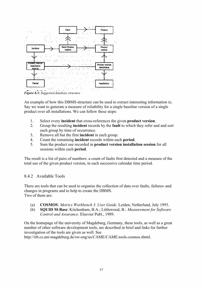
57
Figure 8.3: Suggested database structure
An example of how this DBMS-structure can be used to extract interesting information is;Say we want to generate a measure of reliability for a single baseline version of a singleproduct over all installations. We can follow these steps:
1. Select every incident that cross-references the given product version.2. Group the resulting incident records by the fault to which they refer and and sort
each group by time of occurrence.3. Remove all but the first incident in each group.4. Count the remaining incident records within each period.5. Sum the product use recorded in product version installation session for all
sessions within each period.
The result is a list of pairs of numbers: a count of faults first detected and a measure of thetotal use of the given product version, in each successive calendar time period.
8.4.2 Available Tools
There are tools that can be used to organise the collection of data over faults, failures–andchanges in programs and to help to create the DBMS.Two of them are:
(a) COSMOS: Metrics Workbench 3. User Guide. Leiden, Netherland, July 1993.(b) SQUID M-Base: Kitchenham, B.A.; Littlewood, B.: Measurement for Software
Control and Assurance. Elsevier Publ., 1989.
On the homepage of the university of Magdeburg, Germany, these tools, as well as a greatnumber of other software development tools, are described in brief and links for furtherinvestigation of the tools are given as well. Seehttp://irb.cs.uni-magdeburg.de/sw-eng/us/CAME/CAME.tools.cosmos.shtml.
58
Annotated Bibliography
1 Adams, E., (1984), ‘Optimising Preventive Service of Software Products’, IBMResearch Journal, 28(1), pp 2-14.
2 Akiyama, F., (1971), ‘An Example of Software System Debugging’, Proc. IFIPCongress1971, Ljubljana, Yugoslavia, American Federation of informationProcessing Societies,Montvale, New Jersey.
3 Bache, R., (1990), “Graph Theory Models of Software”, PhD thesis, South BankUniversity, London.
4 Booch, G., (1986), ‘Object Oriented Design’, IEEE Trans.on Softw. Eng. 12(2) pp211-221.
5 Brandl, D.L., (1990), ‘Quality Measures in Design’, ACM Sigsoft SoftwareEngineering Notes, vol 15.
6 Card, D.N., Agresti, W.W., (1988), ‘Measuring Software Design Complexity’, J. ofSys. & Softw. 8, pp 185-197.
7 Conte, S.D., Dunsmore, H.E. and Shen, V.Y., (1986), ‘Software EngineeringMetrics and Models’, Benjamin Cummings Publishing Company Inc.
8 Fenton, N.E., Pfleeger, S. L, (1997), ‘Software Metrics: a Rigorous and PracticalApproach’, Pws Publishing Company, Boston, ISBN: 0-534-95425-1.
9 Glenford, J Myers, (1976), ‘Software Reliability: Principles and Practises’, Wiley& Sons.
10 Halstead, M.H., (1977), ‘Elements of Software Science’, Elsevier/North-Holland,New York.
11 Henry, S., Kafura, D., (1981), “Software Structure Metrics Based on InformationFlow”, IEEE Transactions on Software Engineering, SE-7(5), pp 510-8.
12 Hutton, Les, (1995), ‘Safer C’, McGraw-Hill Book Company, London, ISBN 0-07-707640-0.
13 Ince, D.C., Hekmatpour, S., (1988), “An Approach to Automated Software DesignBased on Product Metrics”, Software Engineering Journal, 3(2), pp 53-6, March.
14 Juran, J.M., (1964), ‘Managerial Breakthrough’, McGraw-Hill, New York.15 Math World–Online Magasine, (2004), last visited march 2004
http://mathworld.wolfram.com/CorrelationCoefficient.html16 McCabe, T.A., (1976), ‘A Complexity Measure’, IEEE Transactions on Software
Engineering, Volume 1 SE-2 pp 308-320, December.17 MISRA, (1995), ’Report 5: Software Metrics’.18 Munson, J.C., Knoshgoftaar T.M., (1992), ‘The Detection of Fault-Prone
Programs’, IEEE Transactions on Software Engineering, 18(5), pp 423-433.19 Nejmeh, B.A., (1988), ‘NPATH: A Measure of Execution Path Complexity and its
Applications’, Comm ACM, 31, (2), pp 188-200.20 Ohlsson, N., (1998), ‘Towards Effective Fault Prevention: an Empirical Study in
Software Engineering’, Linköping University, ISBN 91-7219-176-7.21 Parnas, D.L., (1972), ‘On the Criteria to be Used in Decomposing Systems into
Modules’, CACM 15(2) pp 1053-1058.22 Parnas, D.L., (1979), ‘Designing Software for Ease of Extension and Contraction’,
IEEE Trans. On Softw. Eng. 5(2) pp 128-138.23 Sheppars, M.J., Ince, D.C., (1990), “The Use of Metrics in Early Detection of
Design Errors”, Proceedings of the European Software Engineering Conference ’90,pp 67-85.
24 Shooman, M.L., (1983), ‘Software Engineering’, McGraw-Hill, Singapore.

59
25 Stevens, W.P. Myers, G.J. Constantine, L.L., (1978), ‘Structured Design’, IBM Sys.J. 13(2) pp 115-139.
26 University of Magdeburg, Germany, An Extensive Summery of Available Tools,last visited march 2004.http://irb.cs.uni-magdeburg.de/sw-eng/us/CAME/CAME.tools.cosmos.shtml
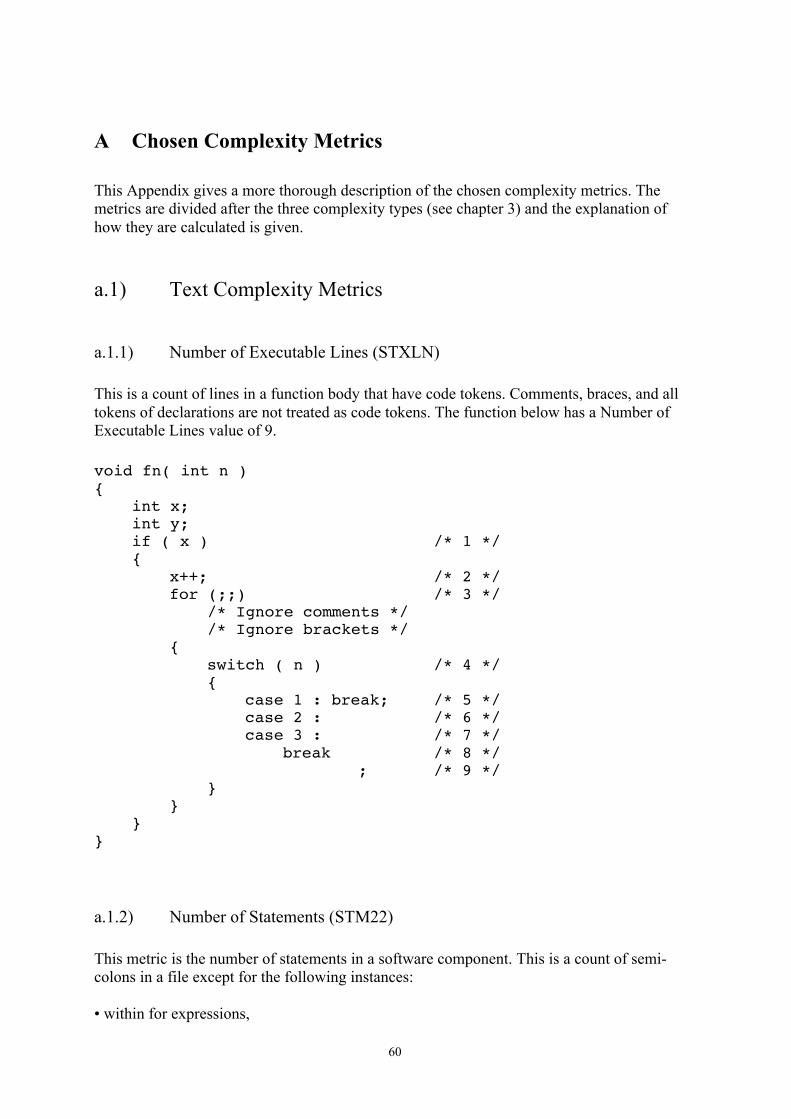
60
A Chosen Complexity Metrics
This Appendix gives a more thorough description of the chosen complexity metrics. Themetrics are divided after the three complexity types (see chapter 3) and the explanation ofhow they are calculated is given.
a.1) Text Complexity Metrics
a.1.1) Number of Executable Lines (STXLN)
This is a count of lines in a function body that have code tokens. Comments, braces, and alltokens of declarations are not treated as code tokens. The function below has a Number ofExecutable Lines value of 9.
void fn( int n ){
int x;int y;if ( x ) /* 1 */{
x++; /* 2 */for (;;) /* 3 */
/* Ignore comments *//* Ignore brackets */
{switch ( n ) /* 4 */{
case 1 : break; /* 5 */case 2 : /* 6 */case 3 : /* 7 */
break /* 8 */; /* 9 */
}}
}}
a.1.2) Number of Statements (STM22)
This metric is the number of statements in a software component. This is a count of semi-colons in a file except for the following instances:
• within for expressions,

61
• within struct or union declarations/definitions,
• within comments,
• within literals,
• within pre-processor directives,
• within old-style C function parameter lists.
The code example below has a Number of Statements (STM22) value of 5.
void f( int a ){
struct { int i; int j; }ij; /* 1 */
a = 1; /* 2 */a = 1; a = 2; /* 3,4 */if
( a > 1 ){
return; /* 5 */}
}
a.2) Component Complexity Metrics
a.2.1) Cyclomatic Complexity (STCYC)
Cyclomatic complexity is calculated as the number of decisions plus 1.
High cyclomatic complexity indicates inadequate modularization or too much logic in onefunction. Some strict programming standards dictate that a function may have a maximumcyclomatic complexity of 10. McCabe (McCabe, 1976) gives an essential discussion of thisissue as well as introducing the metric.
Example 1:
int divide(int x, int y){
if (y != 0) /* 1 */{
return x / y;}else if (x == 0) /* 2 */

62
{return 1;
}else{
printf(stderr, 'div by zero\n');return 0;
}}
The above code sample has a cyclomatic complexity of 3 as there are two decisions made bythe function. Note that correctly indented code does not always reflect the nesting structure ofthe code. In particular the use of the construct else if always increases the level of nesting butis conventionally written without additional indentation and so the nesting is not visuallyapparent.
Example 2:
void how_many(int n){
switch (n){case 0: printf('zero'); /* 1 */
break;case 1: printf('one'); /* 2 */
break;case 2: printf('two'); /* 3 */
break;default: printf('many');
break;}
}
The above code sample has a cyclomatic complexity of 4.
Null statements are treated in the same way as other statement. Switch statements are treatedas if they are dangling if-else statements and else and default are not considered decisions.Multiple conditions in a single branch of a switch statement are collapsed to one decision.For, while, and do statements are treated as though they are simple if statements and arecounted as one decision. The ternary operator (?:) is ignored.
a.2.2) Maximum Nesting of Control Structures (STMIF)
This metric is a measure of the maximum control flow nesting in your source code. You canreduce the value of this metric by turning your nesting into separate functions. This willimprove the readability of the code by reducing both the nesting and the average cyclomaticcomplexity per function.
The code example below has a Maximum Nesting value of 3.

63
int divide(int x, int y){
if (y != 0) /* 1 */{
return (x/y);}else if (x == 0) /* 2 */{
return 1;}else{
printf("Divide by zero\n");while(x > 1) /* 3 */
printf(“x = %i”, x);return 0;
}}
STMIF is incremented in switch, do, while, if and for statements. Note that the nesting levelof code is not always visually apparent by looking at the indentation. In particular, an else- ifconstruct increases the level of nesting in the control flow structure but is conventionallywritten without additional indentation.
a.2.3) Estimated Static Path Count (STPTH)
This is similar to Nejmeh’s NPATH (Nejmeh, 1988) statistic and gives an upper bound on thenumber of possible paths in the control flow of a function. It is the number of non-cyclicexecution paths in a function.
The NPATH value for a sequence of statements at the same nesting level is the product of theNPATH values for each statement and for the nested structures. NPATH is the product of:
• NPATH( sequence of non control statements ) = 1
• NPATH(if) = NPATH(body of then) + NPATH( body of else)
• NPATH(while) = NPATH( body of while) + 1
• NPATH(do while) = NPATH(body of while) + 1
• NPATH(for) = NPATH(body of for) + 1
• NPATH(switch) = Sum( NPATH(body of case 1) ... NPATH(body of case n) )
Note:else and default are counted whether they are present or not.
In switch statements, multiple case options on the same branch of the switch statement bodyare counted once for each independent branch only. For example:

64
switch( n ){
case 0 : break; /* NPATH of this branch is 1 */case 1 :case 2 : break; /* NPATH for case 1 & case 2 */
/* combined is 1 */default: break; /* NPATH for this default is 1 */
}
NPATH cannot be computed if there are goto statements in the function.
The following code example has a static path count of 26.
int n;if ( n ){} /* block 1, paths 1 */
else if ( n ){
if ( n ){} /* block 2, paths 1 */
else{} /* block 3, paths 1 */
/* block 4, paths block2+block3 = 2 */
switch ( n ){case 1 : break;case 2 : break;case 3 : break;case 4 : break;default: break;} /* block 5, paths = 5 */
} /* block 6, paths block4*block5 = 10 */
else{
if ( n ){} /* block 7, paths 1 */
else{} /* block 8, paths 1 */

65
} /* block 9, paths block7+block8 = 2 *//* block 10, paths block1+block6+block9 = 13 */
if ( n ){} /* block 11, paths 1 */
else{} /* block 12, paths 1 *//* block 13, paths block11+block12 = 2 */
/* outer block, paths block10*block13 = 26 */
Each condition is treated as disjoint. In other words, no conclusions are drawn about acondition which is tested more than once. The true path count through a function maytherefore be lower than the static path count, but will never be less than the CyclomaticComplexity.
The true path count through a function usually obeys the inequality:
Cyclomatic Complexity <= true path count <= Static Path Count
a.2.4) Myer's Interval (STMCC)
This is an extension to the Cyclomatic Complexity metric. It is expressed as a pair ofnumbers, conventionally separated by a colon. Myer’s Interval is defined asCyclomatic Complexity: Cyclomatic Complexity + L
Cyclomatic Complexity is a measure of the number of decisions in the control flow of afunction. L is the value of the number of logical operators (&&, ||) in the conditionalexpressions of a function. A large value of L indicates that there are a lot of compounddecisions which make the code more difficult to understand. A Myer’s Interval of 10 isconsidered to be very high.
The example below has a Myer’s interval value of 3:4 because the Cyclomatic Complexity is3 and there is one connective (&&) used in the conditions.
int divide(int x, int y){
if (y != 0) /* Condition 1 */{
return x / y;}else if (x == 0 && y > 2) /* Condition 2 */
/* Conditional expr 1 */{
return 1;}else

66
{printf(stderr, 'div by zero\n');return 0;
}}
In the calculation of Myer’s interval, QA C ignores the ternary operator (?:).
a.3) Structural Complexity Metrics
a.3.1) Number of Function Calls (STSUB)
The number of function calls within a function. Functions with a large number of functioncalls are more difficult to understand because their functionality is spread across severalcomponents. Note that the calculation of Number of Function Calls is based on the number offunction calls and not the number of distinct functions that are called.
A large Number of Function Calls value may be an indication of poor design, a calling treethat spreads too rapidly. See (Brandl, 1990) for a discussion of design complexity and how itis highlighted by the shape of the calling tree.
The following code example has a Number of Function Calls value of 4.
extern dothis(int);extern dothat(int);extern dotheother(int);
void test(){int a, b;a = 1;b = 0;
if (a == 1){
dothis(a); /* 1 */}else{
dothat(a); /* 2 */}
if (b == 1){
dothis(b); /* 3 */}else{
dotheother(b); /* 4 */

67
}}
a.3.2) Estimated Function Coupling (STFCO)
For better explanation of this metric see (Brandl, 1990). Since the actual value of Brandl’smetric requires a full, well-structured calling tree and QA C ca not generate such, this metric,as its name suggests is only an estimate. A high figure indicates a large change of complexitybetween levels of the calling tree. The metric is computed as follows from Number offunction definitions (STFNC) and Number of function calls (STSUB) values of thecomponent functions in the translation unit:
STFCO = ∑(STSUB) - STFNC + 1
The code example below has an STFCO value of 1 (2 - 2 + 1).
BOOL isActive(CHANNEL c);
BOOL okToRead(TEXTCHANNEL c){
return !isActive(c);}
BOOL okToPrint(PRINTCHANNEL c){
return !isActive(c);}

68
B Summary of Demographic Analysis Tables
Summery of Demographic Analysis Tables for CYCLOMATIC COMPLEXITY for thestudied software packages
Percentilevalue
PackageI
PackageII
PackageIII
PackageIV
PackageV
PackageVI
PackageVIII
PackageVII
PackageIX
0 116 89 76 173 90 119 150 144 -5 24 18 39 17 12 21 7 27 -10 17 8 23 9 9 13 4 18 -20 11 5 13 5 4 5 3 11 -30 8 3 7 2 3 3 2 8 -40 6 2 5 2 2 2 1 6 -50 4 2 4 1 1 2 1 5 -60 4 1 3 1 1 2 1 4 -70 3 1 2 1 1 1 1 3 -80 2 1 2 1 1 1 1 2 -90 2 1 1 1 1 1 1 2 -100 2 1 1 1 1 1 1 2 -
Summery of Demographic Analysis Tables for MAXIMUM NESTING OF CONTROLSTRUCTURES for the studied software packages
Percentilevalue
PackageI
PackageII
PackageIII
PackageIV
PackageV
PackageVI
PackageVIII
PackageVII
PackageIX
0 27 32 8 11 10 21 10 15 -5 7 5 5 5 4 9 3 6 -10 5 4 4 4 2 5 2 5 -20 4 2 4 2 1 3 1 4 -30 3 1 3 1 1 2 1 3 -40 3 1 2 1 1 1 0 3 -50 2 1 2 0 0 1 0 2 -60 2 0 1 0 0 1 0 2 -70 1 0 1 0 0 0 0 1 -80 1 0 1 0 0 0 0 1 -90 1 0 0 0 0 0 0 1 -100 1 0 0 0 0 0 0 1 -

69
Summery of Demographic Analysis Tables for ESTIMATED STATIC PATH COUNTfor the studied software packages
Percentilevalue
PackageI
PackageII
PackageIII
PackageIV
PackageV
PackageVI
PackageVIII
PackageVII
PackageIX
0 500 000000
500 000000
500 000000
202 336476
27 885 65 540928
26 662 500 000000
-5 5442 140 31065 95 72 208 8 106272 -10 360 24 388 32 20 50 4 744 -20 53 5 49 6 4 6 3 64 -30 18 3 15 2 4 3 2 20 -40 9 2 5 2 2 2 1 9 -50 6 2 4 1 1 2 1 6 -60 4 1 3 1 1 2 1 4 -70 3 1 2 1 1 1 1 4 -80 2 1 2 1 1 1 1 2 -90 2 1 1 1 1 1 1 2 -100 2 1 1 1 1 1 1 2 -
Summery of Demographic Analysis Tables for NUMBER OF EXECUTABLE LINESfor the studied software packages
Percentilevalue
PackageI
PackageII
PackageIII
PackageIV
PackageV
PackageVI
PackageVIII
PackageVII
PackageIX
0 1414 366 329 384 390 670 512 710 -5 140 63 142 64 55 98 26 136 -10 99 36 84 41 39 55 15 86 -20 60 18 46 17 14 26 8 54 -30 41 10 29 10 8 13 6 37 -40 29 8 19 5 4 10 4 26 -50 21 5 15 3 3 6 4 22 -60 16 2 10 1 2 5 2 16 -70 12 1 7 1 1 3 1 12 -80 10 1 5 1 1 1 1 9 -90 8 1 3 1 1 1 1 6 -100 5 0 0 1 1 0 0 5 -
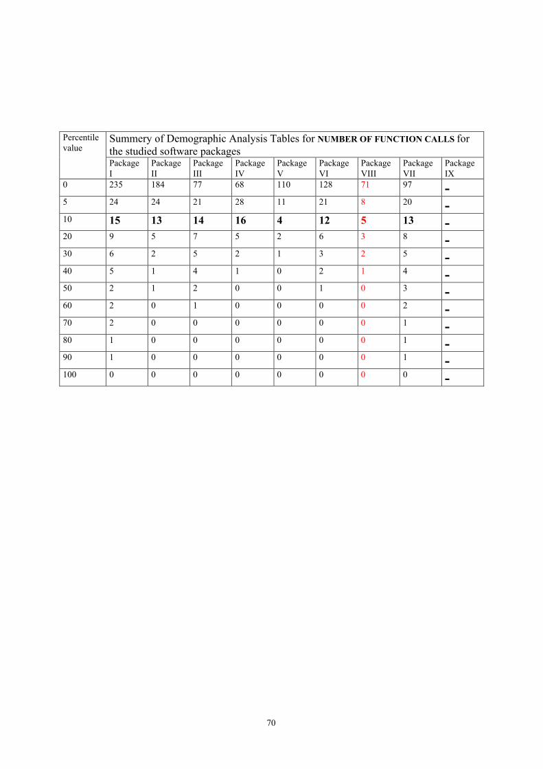
70
Summery of Demographic Analysis Tables for NUMBER OF FUNCTION CALLS forthe studied software packages
Percentilevalue
PackageI
PackageII
PackageIII
PackageIV
PackageV
PackageVI
PackageVIII
PackageVII
PackageIX
0 235 184 77 68 110 128 71 97 -5 24 24 21 28 11 21 8 20 -10 15 13 14 16 4 12 5 13 -20 9 5 7 5 2 6 3 8 -30 6 2 5 2 1 3 2 5 -40 5 1 4 1 0 2 1 4 -50 2 1 2 0 0 1 0 3 -60 2 0 1 0 0 0 0 2 -70 2 0 0 0 0 0 0 1 -80 1 0 0 0 0 0 0 1 -90 1 0 0 0 0 0 0 1 -100 0 0 0 0 0 0 0 0 -

71
C Results of the Survey Investigation
List of the function software metrics that QA C calculates:STAKI Akiyama's Criterion. STLCT Number of local variables declared STPBG Path-based residual bug estimateSTBAK Number of backward jumps STLIN Number of maintainable code lines STPDN Path DensitySTCYC Cyclomatic Complexity STLOP Number of logical operators STPTH Estimated static path countSTELF Number of dangling else-if.s STM07 Essential Cyclomatic Complexity STSUB Number of function callsSTGTO Number of goto.s STM19 Number of Exit Points STUNV Number of unused and unreused variablesSTKDN Knot density STMCC Myer.s Interval STXLN Number of executable linesSTKNT Knot count STMIF Maximum nesting of control structures
Table c.1: Software metrics values for the problematic functionsFunction Name STAKI STBAK STCYC STELF STGTO STKDN STKNT STLCT STLIN STM07Function I 35 0 15 0 0 0 0 8 113 1Function II 97 0 72 1 36 0,1 36 27 473 43Function III 178 0 82 2 44 0,1 44 20 548 54Function IV 241 0 144 10 18 0,03 18 31 941 30Function V 69 0 58 0 0 0 0 6 584 1Function VI 120 0 55 0 0 0,05 14 15 428 27Function VII 35 0 23 0 0 0 0 8 180 1Function VIII 105 0 73 0 0 0 0 24 679 1Function IX 52 0 39 0 0 0,01 2 10 280 1Function X 44 0 42 0 0 0 0 5 262 1Function XI 8 0 7 0 0 0 0 0 57 1Function XII 61 0 40 0 0 0 0 0 268 1Function XIII 38 0 24 0 0 0 0 4 158 1Function XIV 31 0 18 0 0 0 0 3 112 1Function XV 18 0 13 0 0 0,16 13 1 136 3Function XVI 24 0 17 0 0 0 0 1 109 1Function XVII 125 0 76 0 0 0,13 34 10 487 52Function XVIII 145 0 64 0 0 0 1 24 771 1Function XIX 247 0 119 0 0 0 0 42 1105 1Function XX 29 0 9 0 0 0 0 24 182 1Function XXI 76 0 48 0 0 0 0 39 554 1AVERAGE 84,7 0 49,4 0,6 4,7 0 7,7 14,4 401,3 10,7

72
Table c.1 (the extension): Software metrics values for the problematic functionsFunction Name STM19 STMCC STMIF STPBG STPDN STPTH STSUB STUNV STXLNFunction I 0 8 10 2 2,25 119 20 2 53Function II 0 44 14 8 238328,8 88658325 25 0 372Function III 0 56 15 9 1121076 5E+08 96 0 446Function IV 0 50 13 9 704225,4 5E+08 97 1 710Function V 0 74 2 9 1742160 5E+08 11 1 287Function VI 0 35 5 9 1736111 5E+08 65 1 288Function VII 0 11 6 4 46,88 4032 12 0 86Function VIII 0 46 8 7 13445,84 4423680 32 0 329Function IX 2 20 4 4 31,79 4736 13 0 149Function X 0 12 6 5 832,73 118248 2 0 142Function XI 0 7 3 1 0,96 24 1 0 25Function XII 0 0 6 2 0,44 71 21 0 162Function XIII 0 5 4 4 74,43 5508 14 0 74Function XIV 0 0 4 3 6,98 384 13 0 55Function XV 0 1 4 3 4,79 388 5 1 81Function XVI 0 1 5 2 1,87 86 7 0 46Function XVII 0 18 4 8 349648,8 93705885 49 0 268Function XVIII 1 83 13 6 8128,75 2780034 81 0 342Function XIX 0 237 21 7 17623,88 11808000 128 0 670Function XX 0 6 2 2 2,63 192 20 0 73Function XXI 0 30 9 8 176355,6 42854400 28 1 243AVERAGE 0,1 35,4 7,5 5,3 290862,4 1,07E+08 35,2 0,3 233,4

73
Table c.2: Software metrics averages for the program packages & problematic functionsPACKAGES STAKI STBAK STCYC STELF STGTO STKDN STKNT STLCT STLIN STM07 STM19 STMCC STMIF STPBGPackage I 10,5 0 5,6 0 0 0,3 0,5 3,1 62 1 0,5 4,3 2 0,6Package II 5,7 0 3,6 0 0 0 0,1 0,7 20,2 1,1 0,6 0,4 0,9 0,4Package III 10,5 0 4,8 0,1 0 0 0,2 1,3 28,3 1,2 0,6 1,2 1,1 0,4Package IV 9,3 0 4,4 0,1 0 0 0,2 1,0 24,8 1,2 0,5 0,9 1,3 0,5Package V 14,4 0 8,9 0 0 0 0,5 1,3 68,0 1,5 0,3 2,5 2,1 1,1Package VI 7,0 0 4,4 0,1 0,1 0 0,3 0,7 35,9 1,2 0,8 1,7 1,2 0,6Package VII 5,3 0 3,1 0 0 0 0 1,7 29,3 1 0,7 0,9 0,9 0,4AVERAGEPACKAGES 9,0 0,0 5,0 0,0 0,0 0,0 0,3 1,4 38,4 1,2 0,6 1,7 1,4 0,6ALL6 7,1 0,0 4,0 0,0 0,0 0,0 0,2 1,3 31,4 1,1 0,7 1,2 1,1 0,5Problematic_Functions 84,7 0 49,4 0,6 4,7 0 7,7 14,4 401,3 10,7 0,1 35,4 7,5 5,3PF7/ALL 11,9 #DIV/0! 12,2 12,6 238,0 0,0 49,3 11,2 12,8 9,6 0,1 29,6 6,8 11,4PF/AP8 9,5 #DIV/0! 9,9 14,0 329,0 0,0 29,9 10,3 10,5 9,1 0,2 20,8 5,5 9,3
Table c.2 (the extension): Software metrics averages for the program packages& problematic functionsPACKAGES STPDN STPTH STSUB STUNV STXLNPackage I 2071,4 591291,9 4,9 0,1 23,7Package II 1,8 93,2 2 0,1 12Package III 1839,3 516296,3 5,7 0 16,4Package IV 12797,9 2294641,9 4,9 0,1 14,9Package V 34802,1 6082222,5 5,5 0,1 33,8Package VI 15282,6 4971468,6 2,6 0,2 18,8Package VII 4571,2 1353378,9 2,2 0 14,2AVERAGE PACKAGES 10195,2 2258484,8 4,0 0,1 19,1ALL 7754,9 2047352,2 3,1 0,1 16,1Problematic_Functions 290862,4 106874481,5 35,2 0,3 233,4PF/ALL 37,5 52,2 11,4 4,4 14,5PF/AP 28,5 47,3 8,9 3,5 12,2
6 ALL = Average value taken over ALL functions7 PF = Problematic Functions8 AP = Average Packages

74
Table c.3: Complexity metrics averages for the program packages & problematic functions, divided into complexity groups
Text Complexity Component ComplexitySystemComplexity
S & CComplexity
T & CComplexity
PACKAGES STLCT STLIN STXLN STCYC STM07 STMCC STMIF STPBG STPTH STSUB STAKI STPDNPackage I 3,1 62 23,7 5,6 1 4,3 2 0,6 591291,9 4,9 10,5 2071,4Package II 0,7 20,2 12 3,6 1,1 0,4 0,9 0,4 93,2 2 5,7 1,8Package III 1,3 28,3 16,4 4,8 1,2 1,2 1,1 0,4 516296,3 5,7 10,5 1839,3Package IV 1 24,8 14,9 4,4 1,2 0,9 1,3 0,5 2294641,9 4,9 9,3 12797,9Package V 1,3 68 33,8 8,9 1,5 2,5 2,1 1,1 6082222,5 5,5 14,4 34802,1Package VI 0,7 35,9 18,8 4,4 1,2 1,7 1,2 0,6 4971468,6 2,6 7 15282,6Package VII 1,7 29,3 14,2 3,1 1 0,9 0,9 0,4 1353378,9 2,2 5,3 4571,2AVERAGEPACKAGES 1,4 38,4 19,1 5,0 1,2 1,7 1,4 0,6 2258484,8 4,0 9,0 10195,2ALL 1,3 31,4 16,1 4,0 1,1 1,2 1,1 0,5 2047352,2 3,1 7,1 7754,9ProblematicFunctions 14,4 401,3 233,4 49,4 10,7 35,4 7,5 5,3 106874481,5 35,2 84,7 290862,4PF/ALL 11,2 12,8 14,5 12,2 9,6 29,6 6,8 11,4 52,2 11,4 11,9 37,5PF/AP 10,3 10,5 12,2 9,9 9,1 20,8 5,5 9,3 47,3 8,9 9,5 28,5
75
List of the file software metrics that QA C calculates:
STBME COCOMO Embedded Programmer Months STM20 Number of Operand Occurrences STTDO COCOMO Organic Total MonthsSTBMO COCOMO Organic Programmer Months STM21 Number of Operator Occurrences STTDS COCOMO Semi-Detached Total MonthsSTBMS COCOMO Semi-detached Programmer Months STM22 Number of Statements STTLN Total Preprocessed Source LinesSTBUG Residual Bugs (token-based estimate) STM28 Number of Non-Header Comments STTOT Total Number of TokensSTCDN Comment o Code Ratio STM33 Number of Internal Comments STTPP Total Unpreprocessed Source LinesSTDEV Estimated Development Time STMOB Code Mobility STVAR Number of IdentifiersSTDIF Program Difficulty STOPN Halstead Distinct Operands STVOL Program VolumeSTECT Number of External Variables STOPT Halstead Distinct Operators STZIP Zipf Prediction of STTOTSTEFF Program Effort STPRT Estimated Porting TimeSTFCO Estimated Function Coupling STSCT Number of Static VariablesSTFNC Number of Function Definitions STSHN Shannon Information ContentSTHAL Halstead Prediction Of STTOT STTDE COCOMO Embedded Total Months
Table c.4: Software metrics values for the problematic filesFile Name STBME STBMO STBMS STBUG STCDN STDEV STDIF STECT STEFF STFCO STFNC STHAL STM20 STM21 STM22 STM28File I 3,791 2,511 3,148 4 0,806 36,73 11,23 183 220360 63 24 2258 844 1535 273 185File II 6,466 4,006 5,182 9 0,382 137,84 17,43 351 827054 65 49 4685 1786 3421 384 236File III 4,369 2,843 3,594 10 0,957 172,52 6,81 8 1035143 108 13 33383 5238 7939 845 1154File IV 7,698 4,667 6,098 12 0,912 229,67 7,42 4 1378013 9 43 35808 6273 9711 1108 1513File V 6,37 3,955 5,111 12 0,925 227,83 7,32 14 1367006 94 10 37420 6231 9745 1099 1860File VI 15,035 8,383 11,39 15 1,005 293,96 7,63 128 1763779 45 42 45028 7632 11759 1303 2191File VII 31,324 15,934 22,597 12 1,14 210,68 21,21 126 1264087 113 27 4804 2206 4315 491 2352File VIII 9,811 5,771 7,648 17 1,014 364,83 36,66 15 2188974 137 14 3817 2515 4241 531 963File IX 2,904 1,989 2,455 5 1,166 55,08 19,39 2 330451 25 4 2129 742 1340 173 390File X 19,945 10,735 14,828 10 2,521 164,11 20,17 132 984688 213 60 3881 1862 3640 470 2277AVERAGE 10,7713 6,0794 8,2051 10,6 1,0828 189,325 15,527 96,3 1135956 87,2 28,6 17321,3 3532,9 5764,6 667,7 1312,1
Table c.4 (the extension): Software metrics values for the problematic filesFile Name STM33 STMOB STOPN STOPT STPRT STSCT STSHN STTDE STTDO STTDS STTLN STTOT STTPP STVAR STVOL STZIPFile I 143 71,57 264 28 10,44 7 8233 3,829 3,547 3,735 523 2397 1044 222 19631 1826File II 190 88,18 497 43 16,29 8 18115 4,543 4,236 4,446 1092 5227 1629 324 47445 3709File III 785 93,19 2877 56 11,75 2 149586 4,007 3,718 3,912 2037 13203 1175 2031 152074 25109File IV 1057 91,8 3061 61 18,84 7 161484 4,804 4,489 4,707 2682 16007 1884 2248 185813 26922File V 1309 92,94 3184 62 16,09 1 169374 4,521 4,215 4,425 2619 16009 1609 2284 186736 28118File VI 1638 88,8 3763 57 32,91 10 206668 5,951 5,608 5,858 3404 19420 3291 2659 231086 33712File VII 1159 71,2 511 39 60,67 12 18544 7,527 7,159 7,445 1366 6547 6067 333 59599 3788File VIII 633 93,68 421 30 23,06 8 14401 5,192 4,866 5,095 1383 6773 2306 209 59717 3017File IX 265 84,82 249 30 8,36 3 7761 3,516 3,246 3,423 432 2098 836 124 17044 1732File X 603 74,62 426 32 41,65 21 14683 6,515 6,161 6,424 1310 5523 4165 293 48819 3070AVERAGE 778,2 85,08 1525,3 43,8 24,006 7,9 76884,9 5,0405 4,7245 4,947 1684,8 9320,4 2400,6 1072,7 100796,4 13100,3

76
Table c.5: Software metrics averages for the program packages & problematic filesPACKAGES STBME STBMO STBMS STBUG STCDN STDEV STDIF STECT STEFF STFCO STFNC STHAL STM20 STM21 STM22 STM28
Package I 5,7 3,4 4,4 5,6 1,8 82,2 22,6 24,0 493378,1 41,0 10,2 2111,5 801,1 1463,5 169,9 639,6
Package II 3,3 2,0 2,6 9,2 0,9 271,3 27,7 1,6 1627762,5 33,4 22,8 3804,5 1063,2 2022,8 253,8 89,0
Package III 3,0 1,9 2,4 10,0 0,9 297,3 30,7 8,9 1783870,2 76,2 15,8 3490,2 1102,6 2039,7 256,3 83,9
Package IV 5,8 3,4 4,5 17,4 0,3 487,9 38,2 15,1 2927640,2 144,2 35,3 8047,1 2130,6 3870,5 485,4 141,8
Package V 4,6 2,8 3,7 6,4 8,1 129,8 19,8 32,1 778825,5 42,1 12,4 2845,6 908,9 1697,0 222,0 196,4
Package VI 6,5 3,8 5,1 10,6 1,0 210,6 8,6 37,0 1263438,8 33,0 21,1 28557,2 4730,2 7278,0 711,2 1292,1
Package VII 2,9 1,7 2,3 3,3 1,3 53,2 15,7 0,3 318909,9 14,8 10,1 1806,2 561,8 922,0 128,3 120,4AVERAGE PACKAGES 4,5 2,7 3,6 8,9 2,1 218,9 23,3 17,0 1313403,6 54,9 18,3 7237,4 1614,0 2756,2 318,1 366,2ALL 3,8 2,3 3,0 6,3 1,6 140,9 18,6 10,1 845485,4 33,0 14,6 6325,5 1354,3 2233,6 257,7 317,6Problematic_Files 10,8 6,1 8,2 10,6 1,1 189,3 15,5 96,3 1135955,5 87,2 28,6 17321,3 3532,9 5764,6 667,7 1312,1PF/ALL 2,8 2,6 2,7 1,7 0,7 1,3 0,8 9,5 1,3 2,6 2,0 2,7 2,6 2,6 2,6 4,1PF/AP 2,4 2,2 2,3 1,2 0,5 0,9 0,7 5,7 0,9 1,6 1,6 2,4 2,2 2,1 2,1 3,6
Table c.5 (the extension): Software metrics averages for the program packages & problematic filesPACKAGES STM33 STMOB STOPN STOPT STPRT STSCT STSHN STTDE STTDO STTDS STTLN STTOT STTPP STVAR STVOL STZIP
Package I 279,8 77,8 240,6 28,8 12,8 6,0 7824,7 3,9 3,6 3,8 460,7 2277,1 1351,2 120,1 19005,8 1705,9
Package II 73,0 91,6 369,4 31,3 7,5 13,7 15872,9 2,9 2,6 2,8 495,7 3094,3 792,1 96,6 31123,9 2961,8
Package III 68,7 94,4 352,8 34,8 7,2 11,2 14045,1 3,1 2,8 3,0 476,1 3149,8 792,9 112,0 30047,0 2746,5
Package IV 121,6 95,4 769,9 42,0 13,5 26,1 33534,6 3,7 3,5 3,6 942,8 6009,6 1358,1 187,3 61356,5 6198,8
Package V 118,8 72,8 292,6 33,3 10,9 5,8 11264,5 3,6 3,3 3,5 604,5 2615,1 1149,7 121,9 23787,8 2257,8
Package VI 924,4 92,4 2446,6 54,9 15,0 5,8 129008,0 4,1 3,8 4,0 1785,7 12029,0 1529,4 1602,2 138630,4 21490,9
Package VII 89,5 87,3 199,3 22,5 5,7 11,3 6913,3 2,7 2,5 2,7 268,2 1490,2 709,0 102,1 13078,3 1445,2AVERAGE PACKAGES 239,4 87,4 667,3 35,4 10,4 11,4 31209,0 3,4 3,2 3,3 719,1 4380,7 1097,5 334,6 45290,0 5543,9ALL 220,1 88,0 583,6 30,8 8,4 10,8 27344,1 3,1 2,9 3,0 584,2 3597,3 932,8 323,5 37258,9 4843,8Problematic_Files 778,2 85,1 1525,3 43,8 24,0 7,9 76884,9 5,0 4,7 4,9 1684,8 9320,4 2400,6 1072,7 100796,4 13100,3PF/ALL 3,5 1,0 2,6 1,4 2,9 0,7 2,8 1,6 1,6 1,6 2,9 2,6 2,6 3,3 2,7 2,7PF/AP 3,3 1,0 2,3 1,2 2,3 0,7 2,5 1,5 1,5 1,5 2,3 2,1 2,2 3,2 2,2 2,4

77

78
D Results of the Case Study on Package III
List of the function software metrics that QA C calculates:STAKI Akiyama's Criterion. STLCT Number of local variables declared STPBG Path-based residual bug estimateSTBAK Number of backward jumps STLIN Number of maintainable code lines STPDN Path DensitySTCYC Cyclomatic Complexity STLOP Number of logical operators STPTH Estimated static path countSTELF Number of dangling else-if.s STM07 Essential Cyclomatic Complexity STSUB Number of function callsSTGTO Number of goto.s STM19 Number of Exit Points STUNV Number of unused and unreused variablesSTKDN Knot density STMCC Myer.s Interval STXLN Number of executable linesSTKNT Knot count STMIF Maximum nesting of control structures
Table d.1: Correlation coefficients & ranks9 for the function metricsComplexity Metrics STAKI STBAK STCYC STELF STGTO STKDN STKNT STLCT STLIN STM07Correlation Coefficient 0,607 0,000 0,471 0,000 0,000 -0,082 0,170 0,387 0,551 0,254Rank 2 15 6 15 15 18 12 10 3 11
Table d.1 (the extension): Correlation coefficients & ranks for the function metricsComplexity Metrics STM19 STMCC STMIF STPBG STPDN STPTH STSUB STUNV STXLNCorrelation Coefficient -0,149 0,481 0,406 0,458 0,094 0,465 0,640 0,002 0,536Rank 19 5 9 8 13 7 1 14 4
Table d.2: Correlation coefficients & ranks for the relevant function metrics
Complexity Type Text Complexity Component ComplexitySystemComplexity
S & C10
ComplexityT & CComplexity
ComplexityMetrics STLCT STLIN STXLN STCYC STM07 STMCC STMIF STPBG STPTH STSUB STAKI STPDNCorrelationCoefficient 0,387 0,551 0,536 0,471 0,254 0,481 0,406 0,458 0,465 0,640 0,607 0,094Rank 10 3 4 6 11 5 9 8 7 1 2 13
9 Rank represents the size of the correlation coefficient for some complexity metric relative to other correlation coefficients in the table. The higher the rank-number for acomplexity metric, the bigger its correlation coefficient.10 S & C equals System & Component

79
List of the file software metrics that QA C calculates:
STBME COCOMO Embedded Programmer Months STM20 Number of Operand Occurrences STTDO COCOMO Organic Total MonthsSTBMO COCOMO Organic Programmer Months STM21 Number of Operator Occurrences STTDS COCOMO Semi-Detached Total MonthsSTBMS COCOMO Semi-detached Programmer Months STM22 Number of Statements STTLN Total Preprocessed Source LinesSTBUG Residual Bugs (token-based estimate) STM28 Number of Non-Header Comments STTOT Total Number of TokensSTCDN Comment o Code Ratio STM33 Number of Internal Comments STTPP Total Unpreprocessed Source LinesSTDEV Estimated Development Time STMOB Code Mobility STVAR Number of IdentifiersSTDIF Program Difficulty STOPN Halstead Distinct Operands STVOL Program VolumeSTECT Number of External Variables STOPT Halstead Distinct Operators STZIP Zipf Prediction of STTOTSTEFF Program Effort STPRT Estimated Porting TimeSTFCO Estimated Function Coupling STSCT Number of Static VariablesSTFNC Number of Function Definitions STSHN Shannon Information ContentSTHAL Halstead Prediction Of STTOT STTDE COCOMO Embedded Total Months
Table d.3: Correlation coefficients & ranks for the file metricsComplexity Metrics STBUG STDIF STECT STEFF STFCO STFNC STHAL STM20 STM21 STM22 STM28Correlation Coefficient 0,766 0,592 0,724 0,740 0,848 0,652 0,774 0,815 0,833 0,867 0,625Rank 14 21 16 15 4 18 12 8 5 1 19
Table d.3 (the extension): Correlation coefficients & ranks for the file metricsComplexity Metrics STM33 STOPN STOPT STSCT STTLN STTOT STTPP STVAR STVOL STZIPCorrelation Coefficient 0,625 0,776 0,654 0,807 0,864 0,827 0,857 0,766 0,822 0,776Rank 20 11 17 9 2 6 3 13 7 10

80
E Summary of Studied Literature
In this appendix, a short summery is given of some of the books and articles that I studied inorder to get better acquainted with the subject.
Read books:
- Safer C, Hatton L., Mcgraw Hill Book Company, 1995- Software Metrics: A Rigorous & Practical Approach, Fenton N. E. and Pfleeger S. L.,
PWS Publishing Company, 1997- QA C Users Guide, Programming Research Ltd, 2001- Elements of software science, Halstead M. H., Elsevier/North-Holland, New York,
1977
Read articles & repors:
- Report 5: Software Metrics, MISRA, 1995- Complexity Measure, McCabe T. A., IEEE Trans. Software Eng., 1976- Programutvecklingens Grundspel, On Time, Steve McConnell, Nr. 2, june 2003- Software Metrics, http://pan.cie.uce.ac.uk/~G0171941/
Summary
Safer C(Hatton L., Mcgraw Hill Book Company, 1995)
The theme of this book, as said by the writer himself:
The use of C in Safety related or high-integrity systems is not recommended without severe andautomatically enforceable constrains. However if these are present using the formidable tool support forC, the best available evidence suggests that it is then possible to write software of at least as high intristicquality and consistency as with other commonly used languages.
This book attempts to distil these constrains from the vast body of existing experience withthis language into a concise and consistent form of immediate applicability to the C developerand thus attempts to define good working practise.
Software safety, like safety in other engineering disciplines, is about the enforced avoidanceof known problems, the avoidance of needless complexity and the adherence to the simpleand well-established engineering principles which are observed to behave safely.
The central issues are how much of the complexity is justified by the underlying algorithmand how it is distributed. All too often the natural complexity of an algorithm is amplified bypoor implementation to give a corresponding computer program of considerably larger actualcomplexity. Close attention to design can minimize the difference between the actual

81
complexity of the computer program and the natural complexity of the algorithm, which ofcourse, sets the lower bound on the actual complexity, and this indeed is one of the primarygoals of design. This is of the greatest importance, as needless complexity is an old enemy ofgood engineering practise and it is the actual complexity which affects the maintenance costsof software throughout its life cycle.Limiting the complexity of functional software components is believed to improve thereliability and therefore safety of the system.
Metrics are frequently classified into structure metrics, linguistic metrics and hybrid metrics.Linguistic metrics are taken to mean those which consider the program text to be a series oftokens, but which ignore the meaning and order of tokens, such as in the Halstead metrics.One of the main points of this book is to add a new category, deep-flow metrics, which arelinguistically associated but are entirely based on the meaning and order of languagecomponents.
The search for valid complexity measurements of good predictive power has continued foryears, starting with early work of McCabe (1976) and others. Unfortunately not a lot ofprogress seems to have been made so far. In comparison with other measurement sciences,software measurement can be considered at best rudimentary as yet. The measurement ofsoftware properties is widely known as software metrication. There is no shortage of things tomeasure, but there is a dire shortage of case histories which provide useful correlations. Whatis reasonably well established, however, is that there is no single metric which is continuouslyand monotonically related to various useful measures of software quality, such asmaintenance cost, reliability or malleability. It is quite likely that there is not even amonotonic measure of any kind. For example, there is no case what so ever for arguing that aprogram with a cyclomatic complexity of 2 (one decision in a “proper” program) is simplerthan one with cyclomatic complexity of 3 (two decisions). There is however a very reasonablecase for arguing that one with a cyclomatic complexity of 2 is simpler then one with cyc of100. In other words complexity is not strictly monotonic with cyclomatic complexity, but isgenerally monotonic.
As a result, statements concerning the row values of such metrics are of little value owing tothe inadequately understood relationship between the many metrics extant and softwaremaintenance properties in general and there is therefore a need for sensible comparativemeasures to make some progress. Demographic or population analysis concerns theextraction of metrics of proven significance in some context from large population of code.The advantage of this is that it can give such comparative measures of quality, which,although somewhat course, are far more compelling.In essence the values for certain file- or function metric are determined for all files orfunctions in a large population ofsoftware. All metrics evaluated are monotonic in the sensethat higher values are associated with poorer software.Then those files or functions are split up into percentile nod-points as follows:
[a0, a1] contains the worst 10 per cent of all values[a0, a2] contains the worst 20 per cent of all values.[a0, a10] contains the worst 100 per cent of all values
where ai is the appropriate value of the metric.An example of Demographic Analysis results for Cyclomatic Complexity is given below:
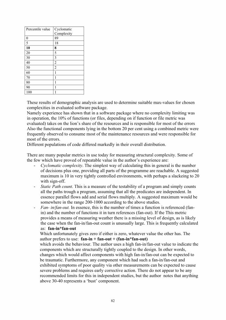
82
Percentile value CyclomaticComplexity
0 895 1810 820 530 340 250 260 170 180 190 1100 1
These results of demographic analysis are used to determine suitable max-values for chosencomplexities in evaluated software package.Namely experience has shown that in a software package where no complexity limiting wasin operation, the 10% of functions (or files, depending on if function or file metric wasevaluated) takes on the lion’s share of the resources and is responsible for most of the errorsAlso the functional components lying in the bottom 20 per cent using a combined metric werefrequently observed to consume most of the maintenance resources and were responsible formost of the errors.Different populations of code differed markedly in their overall distribution.
There are many popular metrics in use today for measuring structural complexity. Some ofthe few which have proved of repeatable value in the author’s experience are:
- Cyclomatic complexity. The simplest way of calculating this in general is the numberof decisions plus one, providing all parts of the programme are reachable. A suggestedmaximum is 10 in very tightly controlled environments, with perhaps a slackeing to 20with sign-off.
- Static Path count. This is a measure of the testability of a program and simply countsall the paths trough a program, assuming that all the predicates are independent. Inessence parallel flows add and serial flows multiply. A suggested maximum would besomewhere in the range 200-1000 according to the above studies.
- Fan- in/fan-out. In essence, this is the number of times a function is referenced (fan-in) and the number of functions it in turn references (fan-out). If the This metricprovides a means of measuring weather there is a missing level of design, as is likelythe case when the fan-in/fan-out count is unusually large. This is frequently calculatedas: fan-in*fan-out
Which unfortunately gives zero if either is zero, whatever value the other has. The author prefers to use: fan-in + fan-out + (fan-in*fan-out) which avoids the behaviour. The author uses a high fan-in/fan-out value to indicate the components which are structurally tightly coupled to the design. In other words, changes which would affect components with high fan-in/fan-out can be expected to be traumatic. Furthermore, any component which had such a fan-in/fan-out and exhibited symptoms of poor quality via other measurements can be expected to cause severe problems and requires early corrective action. There do not appear to be any recommended limits for this in independent studies, but the author notes that anything above 30-40 represents a ‘bust’ component.

83
The switch statement should be taken under special consideration, because it very rapidlybuilds up both the cyclomatic complexity and static path count and yet its homogeneousnature strongly suggests that complexity does not build up linearly. Evidence shows that thecomplexity is more likely to increase logarithmically than linearly, when it increases due tothe Switch statements.
There are a number of other basic data metrics which Hutton suggests exhibit correlation tothe software quality. These include Halsteads metrics, which consider the program text,operands and operators as a stream of tokens, and count of the number of variables havingexternal scope.
Software Metrics: A Rigorous & Practical Approach( Fenton N. E. and Pfleeger S. L., PWS Publishing Company, 1997)
As the name says this book takes on a very rigorous approach on software metrics. It gives acomplete view of the current situation in the field of software metrics, covering all aspects ofit as e.g.: theory of measurements in general, goal-based framework for softwaremeasurement, how to do investigation on correlation in between software metrics anddifferent process and/or product qualities, software-metrics data collection, analyzingsoftware-measurement data, measuring internal product attributes such as size and structureetc.
There were couple of subjects that were of special interest to me. The following is a very briefsummery of those subjects, covering only the most important conclusions:
Empirical investigation
Software practitioners who want to evaluate a technique, method or tool, can use three maintypes of assessment to answer their questions: surveys, case studies and formal experiments.
A survey is a retrospective study of a situation to try to document relationships and outcomes.In software engineering survey you try to pull a set of data from an event that has occurred todetermine how the population reacted to a particular method, tool, or technique, or todetermine trends or relationships. When performing a survey, you have no control over thesituation at hand. That is, because it is a retrospective study, you can record a situation andcompare it with similar ones, but you cannot manipulate variables as you do with experimentsand case studies.
A case study is a research technique where you identify key factors that may affect theoutcome of an activity and then document the activity: its inputs, constraints, resources andoutputs.
By contrast, a formal experiment is a rigorous, controlled investigation of an activity, wherekey factors are identified and manipulated to document their effects on the outcome.
Data Collection

84
Success or failure of any metrics program depends on its underlying data-collection scheme.Precise data to be collected is determined by the particular objectives for measurement. Thereis no universal set of data that can be prescribed. Knowing if your goals are met requirescareful collection of valid and complete data.Data collection should be simple and non-obtrusive, so that developers and maintainers canconcentrate on their primary tasks, with data collection playing a supportive roll. Becausequality is a universal concern, almost all measurement programs require data collection aboutsoftware problems and their resolution. In this book they distinguished among and recordedinformation about, tree types of problems: faults, failures and changes. For each class ofentity a couple of attributes should be recorded:
• Location: where is the entity?• Timing: when did it occur?• Symptom: what was observed?• End result: which consequences resulted?• Mechanism: how did it occur?• Cause: why did it occur?• Cost: how much was incurred by the developer?• Count: how many entities were observed?
Data collection requires a classification scheme, so that every problem is placed in a class,and no two classes overlap. Such a scheme, called an orthogonal classification, allowsanalysis of the types and sources of problems, so that action can be taken to find and fixproblems much earlier in the life cycle.
Analysis of software-measurement data
There were several techniques presented in the book, that addressed a vide variety ofsituations: differing data distribution (e.g. normal or non-normal), varying measurementscales, varying sample sizes, and differing goals. In general, it is advisable to:
• describe a set of attribute values using box plot statistics (based on median andquartiles) rather than on mean and variance;
• inspect a scatter plot visually when investigating the relationship between twovariables;
• use robust correlation coefficients to confirm weather or not a relationship existsbetween two attributes (alternative techniques that can be used are: for normaldistributed values Pearson correlation coefficient, for non-normal data Spearmanrank correlation coefficient or Kendall robust correlation coefficient);
• use robust regression in the presence of atypical values to identify a linearrelationship between two attributes, or remove the atypical values before the analysis(other techniques that can be used are: multivariate regression for more than twovariables and when residuals are not normally distributed Theil’s robust regression);
• always check the residuals by plotting them against the dependent variable;• use Tukey’s ladder to assist in the selection of transformations when faced with non-
linear relationships;• use principal component analysis to investigate the dimensionality of data sets with
large numbers of correlated attributes.
Size metrics

85
Product size can be expressed in many ways. In this book they talk about size beingcomposed of three aspects: length (physical size), functionality (in terms of what the useractually gets) and complexity (of the underlying problem that the software is solving).In many ways the code length is easiest to measure. It can be expressed in terms of: lines ofcode (e.g.: all lines of code, non commented lines of code, executable statements,delivered source instructions etc), number of characters (Halstead’s software sciencemeasures that are defined using number of unique operators/operands and total occurrences ofoperators/operands: length, volume, vocabulary, difficulty, effort and programming time)and more.
Functionality can be derived from specifications by using techniques as: Albrecht’s functionpoints, DeMarco’s specification weight or COCOMO 2.0 object points. Developmentproducts available later in the life cycle can be measured too and compared with earlierestimates. Measures of both length and functionality can be used to normalize other measures,such as expressing defect density in terms of defects per line of code or per function point.Progress and productivity can be tracked in terms of size or functionality of product.
Complexity is difficult to measure and we must distinguish between complexity of theproblem and the complexity of the implemented solution. A theory is presented in the bookthat allows us to define true measures of the efficiency (as an internal attribute) of softwareproducts (namely anything which can be modelled as an algorithm, such as a program or low-level design).
Structure (complexity) metrics
It is widely believed that a well designed software product is characterised largely by itsinternal structure. Indeed, the rationale behind most software engineering methods is to ensurethat software products are built with certain desirable structural attributes. Thus, it isimportant to know how to recognise and measure these attributes, since they may provideimportant indicators of key external attributes, such as: maintainability, testability, reusability,and even reliability.Structural metrics in the book are divided into three groups:
• Control flow metrics, address the sequence in which instructions are executed in aprogram.
• Data flow metrics, follow the trail of data item as it is created or handled by aprogram.
• Data structure metrics, represent the organization of the data itself.
Control flow metrics are in other literature referred to as function-based complexity metrics.This book shows how they all can be computed from a functions prime decomposition, whereprimes are the building blocks of structured programming. The book described the followingcontrol flow metrics in detail: depth of nesting, McCabes cyclomatic number, McCabesessential complexity, VINAP measures, knot measure and a number of test coveragemeasures (number of all paths threw program, number of simple paths, number oflinearly independent paths, etc.)
Data flow metrics are sometimes in literature refered to as file based metrics or inter modularmeasures, since they describe inter module dependencies. They can be divided into:
• global modularity metrics,• morphological metrics (edge to node ratio or tree impurity measure),

86
• internal reuse metrics (system design measure),• coupling metrics (measure of global coupling),• cohesion metrics (cohesion ratio),• information flow metrics (Henry-Kafura information flow complexity, Sheppard
complexity, minimal number of du-paths),
There have been few attempts to define measures of actual data items and their structure. Onesuitable measure proposed in the book is Boehm’s data measure.
QA C-Users Guide(Programming Research Ltd, 2001)
QA C is a deep flow static analyser for C code which is designed to help improve the qualityof software development. It is able to calculate a great deal of software metrics most of whichare correlated with complexity of software. QA C-Manual divides these metrics into twogroups, function based -and file based metrics, and describes how they are calculated andwhat they are used for.
Function-Based Metrics
STAKI Akiyama's Criterion.STBAK Number of backward jumpsSTCYC Cyclomatic ComplexitySTELF Number of dangling else-if.sSTGTO Number of goto.sSTKDN Knot densitySTKNT Knot countSTLCT Number of local variables declaredSTLIN Number of maintainable code linesSTLOP Number of logical operatorsSTM07 Essential Cyclomatic ComplexitySTM19 Number of Exit PointsSTMCC Myer.s IntervalSTMIF Maximum nesting of control structuresSTPBG Path-based residual bug estimateSTPDN Path DensitySTPTH Estimated static path countSTSUB Number of function callsSTUNV Number of unused and unreused variablesSTXLN Number of executable lines
File-Based Metrics
STBME COCOMO Embedded Programmer MonthsSTBMO COCOMO Organic Programmer MonthsSTBMS COCOMO Semi-detached Programmer MonthsSTBUG Residual Bugs (token-based estimate)STCDN Comment o Code RatioSTDEV Estimated Development Time

87
STDIF Program DifficultySTECT Number of External VariablesSTEFF Program EffortSTFCO Estimated Function CouplingSTFNC Number of Function DefinitionsSTHAL Halstead Prediction Of STTOTSTM20 Number of Operand OccurrencesSTM21 Number of Operator OccurrencesSTM22 Number of StatementsSTM28 Number of Non-Header CommentsSTM33 Number of Internal CommentsSTMOB Code MobilitySTOPN Halstead Distinct OperandsSTOPT Halstead Distinct OperatorsSTPRT Estimated Porting TimeSTSCT Number of Static VariablesSTSHN Shannon Information ContentSTTDE COCOMO Embedded Total MonthsSTTDO COCOMO Organic Total MonthsSTTDS COCOMO Semi-Detached Total MonthsSTTLN Total Preprocessed Source LinesSTTOT Total Number of TokensSTTPP Total Unpreprocessed Source LinesSTVAR Number of IdentifiersSTVOL Program VolumeSTZIP Zipf Prediction of STTOT
Elements of Software Science(Halstead M. H., Elsevier/North-Holland, New York, 1977)
This book was one of the earliest attempts to capture notions of size and complexity and hashad a lasting impact on the whole field.Program P is defined as a collection of tokens, classified as either operators or operands. Thebasic metrics for these tokens were:
_1 = number of unique operators_2 = number of unique operandsN1 = total occurrences of operatorsN2 = total occurrences of operands
For example, the FORTRAN statement: A(I) = A(J)Has one operator (=) and two operands (A(I) and A(J)).These metrics are then used to compute a number of other measures of different attributes ofP.
The length of P is defined to be N = N1+ N2, while the vocabulary of P is _ = _1 + _2. Thevolume of the program, akin to the number of mental comparisons needed to write a programof length N, is:
V = N * log2 _The program level of a program P of volume V is

88
L = V*/VWhere V* is the potential volume – the volume of the minimal size implementation of P. Theinverse of level is the difficulty:
D = 1/LAccording to Halstead’s theory, we can calculate an estimate
2
2
1
21ˆND
Lm
m¥==
Likewise, the estimated program length is:
222121 loglogˆ mmmm ¥+¥=NThe effort required to generate P is given by:
2
221
2
logˆ m
mm NN
L
VE ==
where the unit of measurement of E is elementary mental discriminations needed tounderstand P. These relationships are based on those reported in the psychology literature.There, a psychologist named John Stroud claimed that the human mind is capable of making alimited number, _, of elementary discriminations per second. He asserted that 5 ≤ _ ≤ 20.Halstead claimed that _ = 18, and hence the required programming time T for a program ofeffort E is: T = E/18 seconds
MISRA’s report 5: Software Metrics(MISRA, 1995)
The Motor Industry Software Reliability Association (MISRA), gives in Report 5 it is viewon the current situation in the field of software metrics and their relevance for the MotorIndustry.The term “Software metrics is applied to adiverse range of activities including:
• Cost and effort estimation• Productivity measures and models• Quality measures and models• Reliability models• Performance evaluation models• Structural and complexity metrics
MISRA identifies four types of complexity which encompass both software components andsoftware system:
i) text complexity;ii) component complexity;iii) system complexityiv) functional complexity
where only i), ii) and iii) had recognised metrics associated with them, but not iv).
For each of the first three types of complexity a number of metrics was presented, explainedin detail and suitable boundaries (max/min-values) were given.
Text Complexity
89
The text complexity of a software component is closely linked to both the size of thecomponent and to the number of its operands and operators.Some metrics which can be used to analyse the text complexity are:
i) Number of Statements;ii) Number of distinct operands;iii) Number of distinct operators;iv) Number of Operand Occurrences;v) Number of Operator Occurrences;vi) Vocabulary Size;vii) Component Length;viii) Average Statement Size;
Component Complexity
The component Complexity is a measure of the inter-relationships between the statements in asoftware component. Some metrics which can be used to analyse the component complexityare:
i) Cyclomatic number;ii) Number of Decision Statements;iii) Number of Structuring levels;
System Complexity
The system complexity is a measure of the complexity of relationships between softwarecomponents. Some metrics which can be used to analyse the system complexity are:
i) Number of Components;ii) Number of Calling Levels;iii) Number of Calling Paths;iv) Hierarchical complexity;v) Structural Complexity
A Complexity Measure(McCabe T. A., IEEE Trans. Software Eng., 1976)
This paper describes a graph-theoretic complexity measure and illustrates how it can be usedto manage and control program complexity. It has showed that control flow complexity (thecomplexity that addresses the sequence in which instructions are executed in a program) isdependent only on the decision structure of a program and not on the physical size (adding orsubtracting functional statements leaves complexity unchanged).It is one of the earliest papers on the subject and has left a lasting impact on the field ofsoftware complexity metrics.Here is a brief summary of the most interesting results and conclusions from the paper.
Cyclomatic number V(G), where G is its control graph with n vertices, e edges, and pconnected components is:
V(G) = e – n + p Suggested upper bound for cyclomatic complexity is 10 and programmers are advised toeither recognize and modularize subfunctions or redo the software. The only situation in

90
which this limit has seemed unreasonable is when a large number of independent casesfollowed a selection function (a large case statement), which is allowed.Another way (a bit easier for programmer), to calculate cyclomatic number is by countingnumber of predicates (if, while, for, etc) statements plus one.
A measure for the lack of structure, called essential complexity ev was also defined:Ev = v – m
Where v is functions cyclomatic number and m is number of proper subgraphs )in the controlgraph) with unique entry and exit points.A structured program does not contain any parts where branching out of loops, into loops, outof decisions and into decision. Every such ocurrence adds one to essential complexity. Theessential complexity of a structured program is one.
Programutvecklingens grundspel(On Time, Steve McConnell, Nr. 2, juni 2003)
In this article the writer, who himself is a prominent software engineer, tried to sum upopinions and ideas from a debate on importance of software metrics and on their future insoftware development. The debate was waged among some of the top experts in the field andhere is one of the most representative opinions from that debate:
Wolgang: “Oberoende av terminologin (mätetal, eller mätningar), tror jag att detta borde varaytterligare en toppkandidat för de kommande hundra åren. Hur kan vi hävda att vi ärprofessionella om ingen kan mäta några grundläggande fakta relaterade till vårautvecklingsaktiviteter? Hur kan vi hantera aktiviteter som inte kan mätas? Mätningarmisslyckades under 1900-talet inte för att konceptet var dåligt, utan för att arbetsfältetfortfarande befinner sig i sin linda. Det finns inget annat tekniskt arbetsfält som inte skullemäta produkt egenskaper. Och det finns ingen annan tillverkningsaktivitet som inte skulleförsöka mäta resultatet relativt insatserna (vilket är detsamma som produktiviteten). Det ärinte konceptet med mätningar som är fel. Problemet är att konsumenterna har blivit förtoleranta mot bristfällig programvara tillsammans med en överhettad marknad därineffektivitet inte får företag att gå omkull. Om det fanns ett överskott av programutvecklareskulle vi se mycket mer av mätningar som ett sätt att optimera processen.2
Wolfgang Strigel är grundare och VD för Software Productivity Centre i Vancuver Kanada.
Software metrics (the web article)
This article talks very briefly about software metrics in general and Cyclomatic Complexityand Halstead’s theory in a bit more depth. Although it gives a nice general view of mentionedsubjects it does not give any new views or ideas.