predicting aging-related bugs using software complexity

Predicting Aging-Related Bugs using Software

Complexity Metrics

Domenico Cotroneo, Roberto Natella∗, Roberto Pietrantuono

Dipartimento di Informatica e SistemisticaUniversita degli Studi di Napoli Federico II

Via Claudio 21, 80125, Naples, Italy

Abstract

Long-running software systems tend to show degraded performance and an

increased failure occurrence rate. This problem, known as Software Aging,

which is typically related to the runtime accumulation of error conditions, is

caused by the activation of the so-called Aging-Related Bugs (ARBs). This

paper aims to predict the location of Aging-Related Bugs in complex software

systems, so as to aid their identification during testing. First, we carried out

a bug data analysis on three large software projects in order to collect data

about ARBs. Then, a set of software complexity metrics were selected and

extracted from the three projects. Finally, by using such metrics as predictor

variables and machine learning algorithms, we built fault prediction models

that can be used to predict which source code files are more prone to Aging-

Related Bugs.

Keywords: Software Aging, Fault Prediction, Software Complexity

∗Corresponding authorEmail addresses: [email protected] (Domenico Cotroneo),

[email protected] (Roberto Natella), [email protected](Roberto Pietrantuono)

Preprint submitted to Performance Evaluation September 5, 2012

Metrics, Aging-Related Bugs

1. Introduction

Software aging is a phenomenon occurring in long-running software sys-

tems, which exhibit an increasing failure rate as their runtime increases. This

phenomenon is typically related to the accumulation of errors during execu-

tion, that leads to progressive resource depletion, performance degradation,

and eventually to the system hang or crash. This kind of problems has been

observed in several software systems (e.g., web servers, middleware, space-

craft systems, military systems), causing serious damages in terms of loss of

money, or even human lives [1, 2].

Software aging is due to the activation of a particular type of software

faults, called Aging-Related Bugs (ARBs) [3, 4], which tend to cause a failure

only after a long period of execution time. For example, ARBs can mani-

fest themselves as leaked memory, unterminated threads, unreleased files and

locks, numerical errors (e.g., round-off and truncation), and disk fragmenta-

tion.

Due to their nature, it is difficult to observe the effects of such bugs during

testing, and to detect and remove ARBs before the software is released. In

the literature, most research work has been focused on how to mitigate the

negative effects of aging occurrence at runtime. This objective is typically

pursued by estimating the time to aging failure (also referred to as time to

exhaustion), in order to promptly trigger proactive recovery actions to bring

the system in a safe state (e.g., rebooting the system). This strategy is known

as software rejuvenation [5]. The optimal schedule to perform rejuvenation is

2

usually assessed by adopting analytical models and/or by monitoring resource

consumption. It has been demonstrated that rejuvenation is an effective

strategy to mitigate the effects of ARBs, since the scheduled downtime cost

is typically much lower than the cost of an unforeseen downtime caused by a

failure [5]. However, this cost cannot be avoided, and the only approach to

further reduce the system downtime is to prevent the presence of ARBs in

the source code.

Rather than focusing on mitigating the aging effects, this paper is focused

primarily on predicting the location of Aging-Related Bugs in complex soft-

ware systems, in order to aid their identification during testing by assessing

which modules are most probably affected by ARBs. This is an important

concern when developing complex and large systems that are made up of

several thousands of modules and millions of lines of code. The proposed ap-

proach uses source code metrics of software modules as predictive features,

and exploits binary classification algorithms with the goal of identifying the

ARB-prone modules among the ones under test. The prediction can improve

the effectiveness of verification and validation activities, such as code reviews

[6, 7], stress tests [8, 9], and formal methods [10], which can be focused on

the most problematic parts or functionalities of the system.

The driving research hypothesis is that some static software features, such

as the software size, its complexity, the usage of some kinds of programming

structures related to resource management, and other features, might be re-

lated to the presence of ARBs. The underlying principle is that “complexity”

may affect the number of bugs committed by programmers; for instance, it

is more likely for a developer to omit release operations (e.g., to release locks

3

or memory, causing an aging-related bug) in complex and large code than in

a relatively simple and small piece of code; similarly, round-off errors may

be related to the amount of operations, fragmentation to the number of files

opened, and so on.

In order to investigate the relationship between complexity metrics and

ARBs, and thus to confirm/reject the hypothesis, we conducted an empiri-

cal analysis on three large software projects, namely the Linux kernel1, the

MySQL DBMS2, and the CARDAMOM middleware platform for mission-

critical systems3. More specifically, we: (i) manually analyzed the bug re-

ports of these projects to identify ARBs in their individual software modules;

(ii) computed well-known complexity metrics, as well as specific metrics, e.g.,

memory-related ones, defined for this study; (iii) built fault prediction models

using binary classification approaches and the collected data, in order to in-

vestigate whether it is possible to predict ARB-prone modules, and to figure

out which classification model is best suited for this purpose. Results showed

that the ARB-prone files can be effectively predicted (achieving a high per-

centage of detected ARBs and a low percentage of false alarms), especially

when the naive Bayes classifier with logarithmic transformation is adopted.

Moreover, we found that the complexity metrics specifically proposed in this

study (Aging-Related Metrics) contribute to achieve good performance for

all software projects.

The rest of the paper is organized as follows. In Section 2, past work

1Linux kernel 2.6, http://www.kernel.org2MySQL 5.1, http://www.mysql.com3CARDAMOM 3.1, http://cardamom.ow2.org

4

on software aging and software complexity metrics is reviewed. Section 3

describes the software projects considered in this study, and how data about

software complexity metrics and ARBs were collected. Section 4 describes

the classification models adopted in this work. Section 5 presents the detailed

results of the empirical analysis. Section 6 summarizes the findings of the

study.

2. Related work

2.1. Software aging

Software aging has been observed in a variety of systems, such as web

servers [1], telecommunication billing applications [11], military systems [12],

mail severs [13], virtual machines [14, 15], and even in the Linux kernel code

[16].

The term Aging-Related Bug has been formalized by Grottke et al. [3,

17], who distinguished between Bohrbugs, i.e., bugs that are easily isolated

and that manifest consistently under a well-defined set of conditions (its

activation and error propagation lack complexity), and Mandelbugs, i.e., bugs

that are difficult to isolate, and not systematically reproducible (its activation

and/or error propagation are complex). Mandelbugs include the class of

Aging-Related Bugs, i.e., bugs leading to the accumulation of errors either

inside the running application or in its system-internal environment (see also

Section 3.2). A recent analysis of the distribution of bug types has been

conducted in the on-board software of JPL/NASA space missions [4]. The

analysis highlighted that the presence of ARBs is not negligible. They were

found to account for 4.4% of the total bugs found.

5

Besides these recent works on ARBs, the greatest slice of the literature so

far focused on how to mitigate the effects of aging when the system is running,

rather than investigating its causes. To this aim, the basic approach to

counteract aging developed in these years is known as software rejuvenation,

i.e., a proactive approach to environmental diversity that was first proposed

in 1995 by Huang et al. [5]. Its purpose is to restore a “clean state” of the

system by releasing OS resources and removing error accumulation. Some

common examples are garbage collectors (e.g., in Java Virtual Machines) and

process recycling (e.g., in Microsoft IIS 5.0). In other cases, rejuvenation

techniques result in partial or total restarting of the system: application

restart, node reboot and/or activation of a standby spare.

Along this trend, most of research studies on software aging, such as [18,

19, 20], try to the figure out the optimal time for scheduling the rejuvenation

actions. This is typically done by either analytical approaches, in which

the optimal rejuvenation schedule is determined by models [18, 19], or by

measurement-based approaches, in which the optimal schedule is determined

by statistical analyses on data collected during system execution (e.g., the

DBMS performance degradation analysis [21], and the evaluation of Apache

Web Server [1]). Vaidyanathan and Trivedi [20] also proposed a solution

that combines modeling with a measurement-based approach.

Several works have also investigated the dependence of software aging on

the workload applied to the system, such as [22, 23]. These results confirm

that aging trends are related to the workload states. In [24], the authors ad-

dress the impact of application-level workload on aging trends. They apply

the Design of Experiments approach to investigate the effect of controllable

6

application-level workload parameters on aging. Silva et al. [25] highlight

the presence of aging in a Java-based SOAP server, and how it depends on

workload distributions. Our previous work [14, 16] reports the presence of

aging trends both at JVM and OS level; results pointed out the relation-

ship between workload parameters and aging trends (e.g., object allocation

frequency for the JVM, number of context switch for the OS). In [13], we

also analyzed the impact of application-level workload parameters on aging,

such as intensity of requests and size of processed data, and confirmed the

presence of aging in Apache, James Mail Server, and in CARDAMOM, a

middleware for air traffic control systems.

In the work that we carried out in [26], we pursued a different goal: we

investigated the relationship between the static features of the software, as

those expressed by software complexity metrics, and resource consumption

trends. That preliminary study showed that resource consumption trends are

related to the static features of software, although the study was limited by

the assumption that trends are correlated with the number and the severity

of ARBs. The work presented here extends that study: this paper presents

an empirical analysis where software complexity metrics are related to actual

Aging-Related Bugs in the source code, rather than to resource consumption

trends. To achieve this objective, we analyzed a dataset of Aging-Related

Bugs collected from three real-world software projects. We then built fault

prediction models that can be used to predict which source code files are

more prone to Aging-Related Bugs. Finally, several classification models

were evaluated and compared, in order to identify the classifier most suitable

to the purpose of ARB prediction.

7

2.2. Fault prediction

Software metrics have been widely used in the past for predictive and

explanatory purposes. Much work is on investigating relationships between

several kinds of software metrics and the fault proneness in a program. Sta-

tistical techniques are adopted in order to build empirical models, also known

as fault-proneness models, whose aim is to allow developers to focus on those

software modules most prone to contain faults.

In [27], authors used a set of 11 metrics and an approach based on regres-

sion trees to predict faulty modules. In [28], authors mined metrics to predict

the amount of post-release faults in five large Microsoft software projects.

They adopted the well-known statistical technique of Principal Component

Analysis (PCA) in order to transform the original set of metrics into a set

of uncorrelated variables, with the goal of avoiding the problem of redun-

dant features (multicollinearity). The study in [29], then extended in [30],

adopted logistic regression to relate software measures and fault-proneness

for classes of homogeneous software products. Studies in [31, 32] investigated

the suitability of metrics based on the software design. Subsequent studies

confirmed the feasibility and effectiveness of fault prediction using public-

domain datasets from real-world projects, such as the NASA Metrics Data

Program, and using several regression and classification models [33, 34, 35].

In many cases, common metrics provide good prediction results also

across several different products. However, it is difficult to claim that a

given regression model or a set of regression models is general enough to be

used even with very different products, as also discussed in [28, 36]. On the

other hand, they are undoubtedly useful within an organization that itera-

8

tively collects fault data in its process. If a similar relationship is found for

ARBs, developers would better address this phenomenon before the opera-

tional phase, e.g., by tuning techniques for detecting ARBs according to such

predictions.

3. Empirical data

3.1. Case studies

The analysis focuses on three large-scale software projects, namely the

Linux kernel, the DBMS MySQL, and CARDAMOM, a CORBA-based mid-

dleware for the development of mission critical, near real-time, distributed

applications. These are examples of large-scale software used in real-world

scenarios, including business- and safety-critical contexts. MySQL is one of

the most used DBMSs, accounting for a significant market share among IT or-

ganizations [37]. Linux is one of the most prominent examples of open-source

software development, and it is adopted in every domain, from embedded sys-

tems [38] to supercomputers [39]. CARDAMOM is a multi-domain platform,

as it is intended to be used in different industrial domains for Command and

Control Systems (CCS), such as civil Air Traffic Control (ATC) systems, or

Defense Command and Control Systems. Table 1 summarizes the main fea-

tures of the software projects that we analyzed (version, language, number

of files and of physical lines of code at the time of writing).

3.2. Aging-Related Bugs

This Section presents the procedure adopted to identify and collect the

Aging-Related Bugs analyzed in this paper. We rely on the notion of Aging-

9

Table 1: Software projects considered in this study.

Project Version Language Size (LoC) # files

Linux 2.6 C 13.2M 30,039

MySQL 5.1 C/C++ 1.5M 2,272

CARDAMOM 3.1 C++ 847K 4,185

Related Bugs as defined by Grottke et al. [4]. According to that scheme,

bugs can be classified as follows:

• Bohrbugs (BOH): bugs which can be easily isolated. Their activation

and error propagation lack “complexity” (see the explanation below).

• Aging-Related Mandelbugs (ARB): bugs whose activation and/or

error propagation are “complex”, and they are able to cause an increas-

ing failure rate and/or degraded performance.

• Non-Aging-related Mandelbugs (NAM): bugs whose activation and/or

error propagation are “complex”, and are not aging-related.

Aging-Related Bugs are considered a subtype of Mandelbugs. The activa-

tion and/or error propagation are considered “complex” if there is a time lag

between the fault activation and the failure occurrence, or they are influenced

by indirect factors such as the timing and sequencing of inputs, operations,

and interactions with the environment [4]. A bug can be considered as an

ARB if: i) it causes the accumulation of internal error states, or ii) its ac-

tivation and/or error propagation at some instance of time is influenced by

the total time the system has been running.

10

In the case of Linux and MySQL, data about ARBs were collected from

publicly available bug repositories4,5. As for CARDAMOM, no bug reposi-

tory was publicly available at the time of this study. Therefore, we based our

analysis on ARBs found during a testing campaign reported in our previous

study [8]. In order to identify Aging-Related Bugs among all bug reports in

the repositories (for Linux and MySQL), we conducted a manual analysis.

According to the definition of ARBs, the following steps have been carried

out to classify these bugs:

1. extract the information about the activation and the error propagation

from the bug report;

2. if there is not enough information about the activation and the er-

ror propagation to perform the classification (e.g., developers did not

reproduce or diagnose the fault), the fault is discarded;

3. if at least one of them can be considered “complex” (in the sense given

above) and it is aging-related, the fault is marked as Aging-Related

Bug.

The inspection focused on bug reports that are related to unique bugs

(i.e., they are neither duplicates of other reports nor requests for software en-

hancements) and that have been fixed (so that the bug description is reliable

enough to be classified). To this aim, we inspected the reports marked as

CLOSED (i.e., a fix was found and included in a software release). Moreover,

the inspection focused on bug reports related to a specific subset of compo-

4Linux kernel bug repository: http://bugzilla.kernel.org5MySQL DBMS bug repository: http://bugs.mysql.com

11

nents (also referred to as subsystems), since it would be unfeasible to inspect

bug reports for all components of the considered systems. Components were

selected among the most important components of system (i.e., those ones

that are required to make the system work or that are used by most users

of the system), as well as with the goal of covering different functionalities

of the system and a significant share of the system code. We analyzed 4, 3,

and 8 subsystems, respectively for Linux, MySQL, and CARDAMOM. The

subsystems of Linux kernel selected for the analysis are: Network Drivers

(2,043 KLoC), SCSI Drivers (849 KLoC), EXT3 Filesystem (22 KLoC), and

Networking/IPV4 (87 KLoC). Subsystems of MySQL are: InnoDB Storage

Engine (332 KLoC), Replication (45 KLoC), and Optimizer (116 KloC). Ta-

ble 2 provides the number of bug reports from Linux and MySQL (related to

the subsystems previously mentioned) that we analyzed, and the time span

of bug reports; in total, we analyzed 590 bug reports. As for CARDAMOM,

we considered the 8 subsystems that were tested in our previous study [8]:

Configuration and Plugging (3 KLoC), Event (10 KLoC), Fault Tolerance

(59 KLoC), Foundation (40 KLoC), Lifecycle (6 KLoC), Load Balancing (12

KLoC), Repository (27 KLoC), and System Management (142 KLoC).

The analysis identified 36 ARBs in the bug repositories referring to Linux

and MySQL. Additionally, 3 ARBs belong to the CARDAMOM case study.

For each identified ARB, we collected its identification number, a short de-

scription summarizing the report content, the type of ARB, and the source

files that have been fixed to remove the ARB.

Table 3 summarizes the details of the datasets that we obtained in terms

of number of files, their total size, and percentage of ARB-prone files per

12

Table 2: Inspected Bug reports from the Linux and MySQL projects.

Project Time Span Subsystem # Bug Reports

Linux Dec 2003 - May 2011

Network Drivers 208

SCSI Drivers 61

EXT3 Filesystem 33

Networking/IPv4 44

MySQL Aug 2006 - Feb 2011

InnoDB Storage Engine 92

Replication 91

Optimizer 61

dataset. The MySQL dataset includes 261 additional files that do not belong

to a specific component (e.g., header files). Table 4 reports the ARBs that

we found in these projects, along with their type. Most of the ARBs were

related to memory management (e.g., memory leaks). Bugs were marked as

“storage-related” when the ARB consumes disk space (as in the case of the

EXT3 filesystem). Another subset of faults was related to the management

of system-dependent data structures (marked as “other logical resource” in

the table), such as the exhaustion of packet buffers in network drivers’ code.

Finally, ARBs related to numerical errors were a minor part: this is likely due

to the scarcity of floating point arithmetic in the considered projects, which

is not used at all in the case of the Linux kernel [40]. Both “numerical”

ARBs caused the overflow of an integer variable. Appendix A describes

some examples of ARBs.

3.3. Software complexity metrics

As mentioned, the study intends to analyze the relationship between

ARBs and software complexity metrics, for the purpose of fault prediction.

13

Table 3: Datasets used in this study.

Project Size (LoC) # files % ARB-prone files

Linux 3,0M 3,400 0.59%

MySQL 765K 730 2.74%

CARDAMOM 298K 1,113 0.27%

Table 4: Aging-Related Bugs.

Project Subsystem ARB type # ARBs

Linux

Network Drivers

Memory-related 7

Numerical 1

Other logical resource 1

SCSI Drivers Memory-related 4

EXT3 FilesystemMemory-related 3

Storage-related 2

Networking/IPv4Memory-related 1


MySQL

InnoDB Storage Engine

Memory-related 2


Numerical 1

ReplicationMemory-related 4


Optimizer Memory-related 5

CARDAMOM

Configuration and Plugging - -

Event - -

Fault Tolerance - -

Foundation Memory-related 2

Lifecycle - -

Load Balancing Memory-related 1

Repository - -

System Management - -

The software metrics considered6 are summarized in Table 5. We include

6These metrics are automatically extracted by using the Understand tool for static

code analysis, v2.0: http://www.scitools.com14

several metrics that in the past were revealed to be correlated with bug den-

sity in complex software. We aim to evaluate if these metrics are correlated

also with the more specific class of Aging-Related Bugs. Since each target

project encompasses several minor versions (e.g., minor versions 2.6.0, 2.6.1,

etc., in the case of the Linux kernel), we computed the average value of each

complexity metric across all minor versions, in a similar way to [41].

Table 5: Software complexity metrics.

Type Metrics Description

Program size AltAvgLineBlank, AltAvgLineCode, AltAvgLineCom-

ment, AltCountLineBlank, AltCountLineCode, AltCount-

LineComment, AvgLine, AvgLineBlank, AvgLineCode,

AvgLineComment, CountDeclClass, CountDeclFunction,

CountLine, CountLineBlank, CountLineCode, Count-

LineCodeDecl, CountLineCodeExe, CountLineComment,

CountLineInactive, CountLinePreprocessor, CountSemi-

colon, CountStmt, CountStmtDecl, CountStmtEmpty,

CountStmtExe, RatioCommentToCode

Metrics related to

the amount of lines

of code, declara-

tions, statements,

and files

McCabe’s cyclo-

matic complexity

AvgCyclomatic, AvgCyclomaticModified, AvgCyclomatic-

Strict, AvgEssential, MaxCyclomatic, MaxCyclomatic-

Modified, MaxCyclomaticStrict, SumCyclomatic, SumCy-

clomaticModified, SumCyclomaticStrict, SumEssential

Metrics related to

the control flow

graph of functions

and methods

Halstead metrics Program Volume, Program Length, Program Vocabulary,

Program Difficulty, Effort, N1, N2, n1, n2

Metrics based on

operands and opera-

tors in the program

Aging-Related

Metrics (ARMs)

AllocOps, DeallocOps, DerefSet, DerefUse, UniqueDeref-

Set, UniqueDerefUse

Metrics related to

memory usage

The first subset of metrics is related to the “size” of the program in terms

of lines of code (e.g., total number of lines, and number of lines containing

15

comments or declarations) and files. These metrics provide a rough estimate

of software complexity, and they have been used as simple predictors of fault-

prone modules [33]. In addition, we also consider other well-known metrics,

namely McCabe’s cyclomatic complexity and Halstead metrics [42]. These

metrics are based on the number of paths in the code and the number of

operands and operators, respectively. We hypothesize that these metrics are

connected to ARBs, since the complexity of error propagation (which is the

distinguishing feature of ARBs [4]) may be due to the complex structure of

a program.

Finally, we introduce a set of metrics related to memory usage (Aging-

Related Metrics, ARMs), that we hypothesize to be related with aging since

most of ARBs are related to memory management and handling of data struc-

tures (see also Table 4). The AllocOps and DeallocOps metrics represent the

number of times a memory allocation or deallocation primitive is referenced

in a file. Since the primitives adopted for memory allocation and dealloca-

tion vary across the considered software projects, these metrics were prop-

erly tuned for the system under analysis: the malloc and new user-library

primitives are adopted for allocating memory in MySQL and CARDAMOM;

instead, Linux is an operating system kernel and therefore it adopts kernel-

space primitives, such as kmalloc, kmem cache alloc, and alloc page [40]. The

DerefSet and DerefUse metrics represent the number of times a pointer vari-

able is dereferenced in an expression, respectively to read or write the pointed

variable. The UniqueDerefSet and UniqueDerefUse have a similar meaning

as DerefSet and DerefUse; however, each pointer variable is counted only

one time per file. These metrics can potentially be expanded to consider

16

system-specific features (e.g., files and network connections), although we

only consider metrics related to memory usage due to the predominance of

memory-related ARBs and to their portability across projects.

4. Classification models

Since modern software is typically composed by several thousand mod-

ules with complex relationships between them, as in the case of the software

projects considered in this work (see also Table 3), the process of locat-

ing ARBs should be automated as much as possible. As mentioned in the

previous sections, we assess whether it is possible to locate ARBs by using

software complexity metrics. Since the relationship between software metrics

and ARBs is not self-evident and depends on the specific problem under anal-

ysis, we adopt machine learning algorithms to infer this relationship, which

are widely applied to knowledge discovery problems in industry and science

where large and complex volumes of data are involved [43].

In particular, we formulate the problem of predicting the location of ARBs

as a binary classification problem. Binary classification consists in learning a

predictive model from known data samples in order to classify an unknown

sample as “ARB-prone” or “ARB-free”. In this context, a data sample is

represented by a program unit in which software faults may reside. In par-

ticular, files (also referred to as modules in the following) are the basic unit

of our analysis: they are small enough to allow classifiers to provide precise

information about where ARBs are located [33], and they are large enough

to avoid sparse and excessively large datasets. We did not focus on predict-

ing the exact number of ARBs per file, but only on the presence or absence

17

of ARBs in a file, since the percentage of files with strictly more than one

ARB is extremely small, amounting to 0.19% of data samples (this is a fre-

quent situation in fault prediction studies [35]). In this section, we briefly

describe the classification algorithms (also referred to as classifiers) adopted

in this study. These algorithms, which are trained with examples, try to

extract from samples the hidden relationship between software metrics and

“ARB-prone” modules. We consider several algorithms in this study, since

they make different assumptions about the underlying data that can signifi-

cantly affect the effectiveness of fault prediction. We focus on classification

algorithms that could be easily adopted by practitioners and that require to

manually tune only few or no parameters. Classification algorithms are then

evaluated and compared in Section 5.

4.1. Naive Bayes

A Naive Bayes (NB) classifier is based on the estimation of a posteriori

probability of the hypothesis H to be assessed (e.g., “a module is ARB-

prone”). In other words, it estimates the probability that H is true given

that an evidence E has been observed. The a posteriori probability can be

obtained by combining the probability to observe E under the hypothesis H,

and the a priori probabilities of the hypothesis H (i.e., the probability P (H)

when no evidence is available) and of evidence E:

P (H|E) =P (E|H)P (H)

P (E). (1)

The evidence E consists of any information that is collected and ana-

lyzed for classification purposes. Many sources of information are typically

18

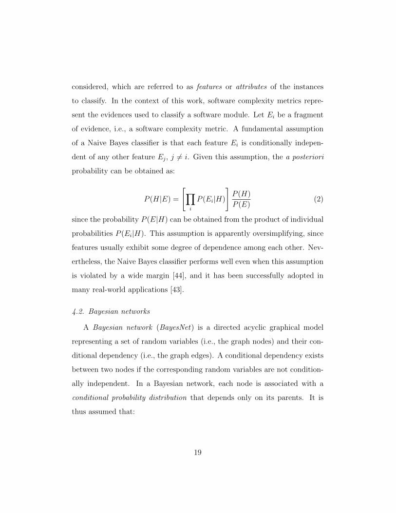
considered, which are referred to as features or attributes of the instances

to classify. In the context of this work, software complexity metrics repre-

sent the evidences used to classify a software module. Let Ei be a fragment

of evidence, i.e., a software complexity metric. A fundamental assumption

of a Naive Bayes classifier is that each feature Ei is conditionally indepen-

dent of any other feature Ej, j 6= i. Given this assumption, the a posteriori

probability can be obtained as:

P (H|E) =

[∏i

P (Ei|H)

]P (H)

P (E)(2)

since the probability P (E|H) can be obtained from the product of individual

probabilities P (Ei|H). This assumption is apparently oversimplifying, since

features usually exhibit some degree of dependence among each other. Nev-

ertheless, the Naive Bayes classifier performs well even when this assumption

is violated by a wide margin [44], and it has been successfully adopted in

many real-world applications [43].

4.2. Bayesian networks

A Bayesian network (BayesNet) is a directed acyclic graphical model

representing a set of random variables (i.e., the graph nodes) and their con-

ditional dependency (i.e., the graph edges). A conditional dependency exists

between two nodes if the corresponding random variables are not condition-

ally independent. In a Bayesian network, each node is associated with a

conditional probability distribution that depends only on its parents. It is

thus assumed that:

19

P (node|parents plus any other nondescendants) = P (node|parents). (3)

The joint probability distribution for a set of random variables X1, . . . , Xn

of the Bayesian network (which can be ordered to give all ancestors of a node

Xi indices smaller than i) can be expressed as:

P (X1, . . . , Xn) =n∏

i=1

P (Xi|Xi−1, . . . , X1) =n∏

i=1

P (Xi|Xi’s parents). (4)

Equation 4 can be used to compute the probability of a hypothesis H

represented by a node of the network, given the conditional probability dis-

tributions of each node, and given a set of observed values. In this study,

a Bayesian network is made up of nodes that represent software complexity

metrics and the hypothesis “a module is ARB-prone”. A Bayesian network

represents a more accurate model than a naive Bayes classifier, since it makes

weaker assumptions about independence of random variables: in a Bayesian

network model, the structure of the network and the conditional probability

distributions can be tuned to model complex dependency relationships be-

tween random variables. A Bayesian network is considerably more complex

to build than a naive Bayes classifier, since both the network structure and

conditional probability distributions have to be inferred from the data. In

this work, we consider a simple and common algorithm for building Bayesian

networks, namely K2 [43]. This algorithm processes each node in turn and

greedily considers adding edges from previously processed nodes to the cur-

rent one. In each step it adds the edge that maximizes the probability of the

20

data given the network. When there is no further improvement, attention

turns to the next node. Because only edges from previously processed nodes

are considered, this procedure cannot introduce cycles. Since the result de-

pends on the order by which nodes are inspected, the algorithm should be

executed several times with different node orderings in order to identify the

best network structure.

4.3. Decision trees

A decision tree (DecTree) is a hierarchical set of questions that are used to

classify an element. Questions are based on attributes of elements to classify,

such as software complexity metrics (e.g., “is LoC greater than 340?”). A

decision tree is obtained from a dataset using the C4.5 algorithm [43]. The

C4.5 algorithm iteratively splits the dataset in two parts, by choosing the

individual attribute and a threshold that best separates the training data

into the classes; this operation is then repeated on the subsets, until the

classification error (estimated on the training data) is no further reduced.

The root and inner nodes represent questions about software complexity

metrics, and leaves represent class labels. To classify a component, a metric

of the component is first compared with the threshold specified in the root

node, to choose one of the two children nodes; this operation is repeated for

each selected node, until a leaf is reached.

4.4. Logistic regression

Regression models represent the relationship between a dependent vari-

able and several independent variables by using a parameterized function. In

21

the case of logistic regression, the relationship is given by the function

P (Y ) =ec+a1X1+...+anXn

1 + ec+a1X1+...+anXn(5)

where the features X1, . . . , Xn are independent variables, and c and a1, . . . , an

are parameters of the function. This function is often adopted for binary

classification problems since it assumes values within the range [0, 1], which

can be interpreted as the probability to belong to a class. The function

parameters have to be tuned in order to model the data properly. The model

can be trained using one of several numerical algorithms: a simple method

consists in iteratively solving a sequence of weighted least-squares regression

problems until the likelihood of the model converges to a maximum.

5. Data analysis

The effectiveness of ARB prediction is assessed by training a classification

model using empirical data (namely training set), and by using this model to

classify other data that have not been used during the training phase (namely

test set), in order to estimate the ability of the approach to correctly predict

ARB-proneness of unforeseen data instances. These sets are obtained from

the available dataset (described in Section 3) by dividing it between a training

set and a test set. The division is performed in several ways to evaluate the

approach in different scenarios, which are discussed in the following of this

Section.

For each data sample in the test set, the predicted class is compared

with the actual class of the sample. We denote the samples of the test set

belonging to the target class (i.e., “a module is ARB-prone”) as true positives

22

if they are correctly classified, and as false negatives if they are not correctly

identified. In a similar way, the samples belonging to the other class (i.e.,

“a module is ARB-free”) are denoted as true negatives if they are correctly

classified, and as false positives otherwise. We adopt performance indicators

commonly adopted in machine learning studies [43], including works on fault

prediction [33, 34, 35]:

• Probability of Detection (PD). It denotes the probability that a

ARB-prone module will actually be identified as ARB-prone. A high

PD is desired in order to identify as many ARB-prone modules as

possible. PD is defined as:

PD =true positives

true positives + false negatives· 100 [%]. (6)

• Probability of False alarms (PF). It denotes the probability that a

non-ARB-prone module is erroneously identified as ARB-prone. A low

PF is desired in order to avoid the cost of verifying a module that is

not ARB-prone. PF is defined as:

PF =false positives

true negatives + false positives· 100 [%]. (7)

• Balance (Bal). PD and PF are usually contrasting objectives (e.g.,

a classifier with high PD can also produce several false positives and

therefore high PF), and a trade-off between them is needed for any

practical purpose. Bal is based on the Euclidean distance from the

ideal objective PD = 100[%] and PF = 0[%] [34], and it is defined as:

23

Bal = 100−√

(0− PF )2 + (100− PD)2

√2

. (8)

It should be noted that there exist other performance indicators that

can be obtained from true/false positives/negatives, such as the precision

of a classifier, which is the percentage of true positives among all modules

identified as ARB-prone, and its harmonic average with PD, namely the

F-measure. We do not consider these measures since precision provides un-

reliable rankings for datasets where the target class occurs infrequently (as

showed in [45]), like the ones considered in this study. In fact, precision is in-

sensitive to variations of PD and of PF when the percentage of ARB-prone

files is very low, which makes precision unsuitable for comparing different

algorithms. However, in the following we also discuss problems related to

precision, and this measure can be derived from the data provided in this

section using [45, eq. 1]. Other performance indicators not included here,

such as the Receiver Operational Characteristic, provide similar information

to the PD and PF measures since they describe the performance of a clas-

sifier in the PD,PF space.

We first evaluate fault prediction when data about ARBs in the project

under analysis is available, that is, ARB-proneness of a set of files is predicted

by training a classification model using files (of which ARB-proneness is

already known) from the same project, such as past versions of the files

under analysis or different files that were already tested. In order to perform

this evaluation, we split the dataset of a given project in two parts: a training

set representing the files for which ARB-proneness is known, and a test set

representing the files to be classified [34]. We assume that the training set

24

is representative of data available to developers that collect historical data

about ARBs of a software system with a long lifecycle, since the datasets

have been obtained by analyzing real bug reports of large, long-life software

systems over a large time period (see Table 2).

Since results can be affected by the selection of the data samples used for

the training and test sets, the evaluation has to be repeated several times

using different, randomly-selected training and test sets. This approach,

which is referred to as cross-validation [43], repeats the evaluation N times

for each classifier (NB, BayesNet, DecTree, Logistic) and for each dataset

(Linux, MySQL, CARDAMOM ), and computes the average results. In each

repetition, 66% of the random samples are used for the training set and the

remaining for the test set. In order to assure that the number of repetitions is

sufficient to obtain reliable results, we computed the 95% confidence interval

of the measures using bootstrapping [46]. Given a set of N repeated measures,

they are randomly sampled M times with replacement (we adopt M = 2000),

and the measure is computed for each sample in order to obtain an estimate of

the statistical distribution of the measure and of its 95% confidence interval.

The number of repetitions is considered sufficient if the error margin of the

estimated measure (i.e., the half-width of the confidence interval) is less than

5%. We performed N = 100 repetitions, which resulted to be sufficient to

satisfy this criterion.

Table 6 provides the average results for each dataset and for each classifier

using cross-validation. Classification experiments were performed using the

WEKA machine learning tool [43]. Each classifier was evaluated both on

the plain datasets without preprocessing (e.g., “NB”), and on the datasets

25

preprocessed with a logarithmic transformation (e.g., ”NB + log”). The

logarithmic transformation replaces each numeric value with its logarithm;

if the value is zero or extremely small (< 10−6), the value is replaced with

ln(10−6). This transformation can improve, in some cases, the performance

of classifiers when attributes exhibit many small values and a few much larger

values [34]. Aging-Related Metrics are not considered at this stage.

We performed a hypothesis test to identify the best classifier(s), in order

to assure that differences between classifiers are statistically significant, i.e.,

the differences are unlikely due to random errors. In particular, we adopted

the non-parametric Wilcoxon signed-rank test [47]. This procedure tests the

null hypothesis that the differences Zi between repeated measures from two

classifiers have null median (e.g., when comparing the PD of the NB and

Logistic classifiers, Zi = PDNB,i − PDLogistic,i, i = 1 . . . N). The procedure

computes a test statistic based on the magnitude and the sign of the dif-

ferences Zi. Under the null hypothesis, the distribution of the test statistic

tends towards the normal distribution since the number of samples is large

(in our case, N = 100). The null hypothesis is rejected (i.e., there is a

statistically significant difference between classifiers) if the p-value (i.e., the

probability that the test statistic is equal to or greater than the actual value

of the test statistic, under the null hypothesis and the normal approxima-

tion) is equal to or lower than a significance level α. This test assumes that

the differences Zi are independent and that their distribution is symmetric;

however, the samples are not required to be normally distributed, and the

test is robust when the underlying distributions are non-normal. For each

column of Table 6, we highlight in bold the best results according to the

26

Wilcoxon signed-rank test, with a significance level of α = 0.05. For some

datasets and performance indicators, more than one classifier may result to

be the best one.

Table 6: Comparison between classifiers.

AlgorithmLinux MySQL CARDAMOM

PD PF Bal PD PF Bal PD PF Bal

NB 60.13 12.46 69.24 49.14 10.46 63.02 0.00 7.18 29.08

NB + log 92.66 37.09 72.28 88.30 34.67 73.53 54.50 25.15 53.25

BayesNet 3.72 1.85 31.91 44.57 8.65 60.26 0.00 0.00 29.30

BayesNet + log 5.34 1.95 33.06 44.50 8.65 60.21 0.00 0.00 29.30

DecTree 0.00 0.03 29.30 11.21 2.64 37.17 0.00 0.00 29.30

DecTree + log 0.00 0.00 29.30 11.28 2.65 37.22 0.00 0.00 29.30

Logistic 1.00 0.63 30.01 22.93 4.43 45.40 0.00 1.21 29.30

Logistic + log 3.84 0.62 32.01 25.07 5.13 46.88 0.00 0.65 29.30

Table 6 points out that the naive Bayes classifier with logarithmic trans-

formation is the best classifier for the Linux and MySQL datasets with re-

spect to PD (i.e., it correctly identifies the highest percentage of ARB-prone

files). In all the cases except the naive Bayes classifier with and without

logarithmic transformation, PD < 50% (i.e., most of ARB-prone files are

missed). The high PD comes at the cost of a non-negligible amount of false

positives (i.e., PF is higher that other classifiers). This fact is consistent with

other studies on fault prediction [33, 34, 35]: in order to detect ARB-prone

modules, classifiers have to generalize from samples and can make mistakes

in doing so. This problem is exacerbated by the high skew towards ARB-free

modules in our datasets (Table 3), since it is a challenging problem for a

classifier to be so precise to identify few ARB-prone files without incurring

27

non-ARB-prone files [35]. As a result, the precision of classifiers tends to be

low, that is, there are several false positives among the modules flagged as

ARB-prone (actually, less than 25% are ARB-prone). However, the predic-

tion is useful even if precision is low. For instance, a classifier that generates

false positives in 33% of cases (and thus has a low precision due to the small

percentage of ARB-prone files), and that detects most of the ARB-prone

files, is useful to improve the efficiency of the V&V process, since it avoids to

test or to inspect the remaining 67% of non-ARB-prone files (true negatives).

The high Bal values highlight that the “NB + log” classifier provides the

best trade-off between PD and PF . The reason for the low performance of

other classifiers is that they are negatively affected by the small percentage

of ARB-prone files in the datasets [35].

The classifiers were less effective in the case of the CARDAMOM dataset

compared to the Linux and MySQL datasets. The only classifier able to

achieve PD > 0% is naive Bayes, although PD is lower than the cases of

Linux and MySQL. The same result was also observed for the Bal indicator.

This is likely due to the fact that the CARDAMOM dataset is even more

skewed than the other datasets (Table 3).

Since classification performance can be affected by the selection of soft-

ware complexity metrics included in the model (for instance, discarding a

redundant metric could improve performance), we analyze what is the im-

pact of attribute selection. In particular, we consider the Information Gain

Attribute Ranking algorithm [48, 49], in which attributes are ranked by their

information gain, which is given by:

28

0 5 10 15 20 25 30 35 40 45

0

10

20

30

40

50

60

70

80

90

Number of attributes

PD, P

F, B

al (%

)

BalPDPF

Top 10 metrics

AvgLineComment

AltAvgLineComment

AvgLine

AvgCyclomaticModified

SumCyclomaticStrict

Dif

CountLineComment

SumEssential

AltCountLineComment

AvgCyclomatic

Figure 1: Impact of attribute selection on Linux.

InfoGain(Ai) = H(C)−H(C|Ai)

= −∑c∈C

P (c) · log2 P (c)−

− ∑a∈D(Ai)

P (a)∑c∈C

P (c|a) · log2 P (c|a)

.(9)

where H() denotes the entropy, C = {ARB-prone, non-ARB-prone}, D(Ai)

is the set of values7 of attribute Ai, and the information gain measures the

number of bits of information obtained by knowing the value of attribute Ai

[49].

The sensitivity of performance indicators of “NB + log” with respect to

the size of the attribute set (i.e., the top n attributes ranked by information

7Numeric data are discretized in 10 bins.

29

0 5 10 15 20 25 30 35 40 45

0

10

20

30

40

50

60

70

80

90


PD, P

F, B

al (%

)

BalPDPF

Top 10 metrics

CountLineBlank

CountLineCode

CountStmt

AltCountLineBlank

CountSemicolon

MaxCyclomaticModified

AltCountLineCode

CountStmtEmpty

MaxCyclomatic

CountLineComment

Figure 2: Impact of attribute selection on MySQL.

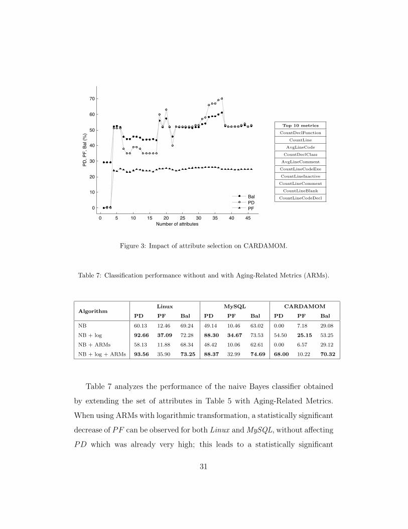
gain, for increasing values of n) is showed in Figure 1, Figure 2, and Figure 3

for the three projects. It can be seen that at least 5 metrics are required to

achieve a high probability of detection for all datasets. The CARDAMOM

project is the most sensitive to the number of attributes with respect to

PD and PF , although the balance stabilizes when more than 5 metrics

are considered. It can be observed that there is no individual metric that

can be used alone for classification, but the best performance is obtained

when considering several metrics and letting the classifier ascertain how to

combine these metrics. Since the impact of attribute selection on classifier

performance is small (i.e., considering 5 metrics gives similar results to the

full set of metrics), we do not apply attribute selection in the subsequent

analyses.

30

0 5 10 15 20 25 30 35 40 45

0

10

20

30

40

50

60

70


PD, P

F, B

al (%

)

BalPDPF

Top 10 metrics

CountDeclFunction

CountLine

AvgLineCode

CountDeclClass

AvgLineComment

CountLineCodeExe

CountLineInactive

CountLineComment

CountLineBlank

CountLineCodeDecl

Figure 3: Impact of attribute selection on CARDAMOM.

Table 7: Classification performance without and with Aging-Related Metrics (ARMs).

AlgorithmLinux MySQL CARDAMOM


NB 60.13 12.46 69.24 49.14 10.46 63.02 0.00 7.18 29.08

NB + log 92.66 37.09 72.28 88.30 34.67 73.53 54.50 25.15 53.25

NB + ARMs 58.13 11.88 68.34 48.42 10.06 62.61 0.00 6.57 29.12

NB + log + ARMs 93.56 35.90 73.25 88.37 32.99 74.69 68.00 10.22 70.32

Table 7 analyzes the performance of the naive Bayes classifier obtained

by extending the set of attributes in Table 5 with Aging-Related Metrics.

When using ARMs with logarithmic transformation, a statistically significant

decrease of PF can be observed for both Linux and MySQL, without affecting

PD which was already very high; this leads to a statistically significant

31

increase of Bal. The greatest benefit is obtained for CARDAMOM : the naive

Bayes with logarithmic transformation and ARMs provides PD = 68% and

reduces PF at the same time, therefore achieving much better performance.

In this specific case, the AllocOps metric is responsible for the improvement

of prediction. This metric contributes to ARB prediction since ARBs in

CARDAMOM are all related to misuses of the new C++ operator. However,

it should be noted that ARMs for ARB-prone files in this project do not take

on values far from the average values, and that the AllocOps metric alone is

not sufficient to identify ARB-prone files but it has to be combined with non-

aging-related metrics in order to achieve good performance. In conclusion,

since ARMs improved ARB prediction in all three projects (reducing PF

in every case and increasing PD in CARDAMOM), these metrics can be

considered a useful support for predicting this category of bugs and should

be adopted wherever possible.

Table 8: Cross-component classification in Linux.

ComponentLinux

PD PF Bal

Network drivers 88.9 41.7 69.5

SCSI drivers 75.0 27.6 73.7

EXT3 100.0 29.2 79.4

IPv4 100.0 52.2 63.1

Finally, we analyze the effectiveness of the naive Bayes classifier when

training data about ARBs in the component or project under analysis are

not available. In such scenarios, training data from different components

of the same project, or from different projects should be adopted. In these

32

Table 9: Cross-component classification in MySQL.

ComponentMySQL

PD PF Bal

InnoDB 65.6 16.5 73.0

Replication 100.0 28.6 79.8

Optimizer 100.0 69.7 50.7

Table 10: Cross-component classification in CARDAMOM.

ComponentCARDAMOM

PD PF Bal

Foundation 0.0 0.0 29.3

Load Balancing 100.0 9.0 93.7

cases, the test set is made up of data from the target component (respectively,

target project), and the training set is made up of data from the remaining

components of the same project (respectively, from the remaining projects).

This evaluation process is repeated several times, each time with a different

target component or target project. It should be noted that this evaluation

process does not require to randomly split data between a training and a

test set (this was the case of cross-validation), since the training and the test

data are determined by component/project boundaries. First, we analyze

the scenario in which a classifier has to be deployed for a specific component

for which data is unavailable, and the classifier is built using data from

the remaining components. The logarithmic transformation and ARMs are

adopted.

Table 8, Table 9 and Table 10 show the results for each dataset. In the

33

case of CARDAMOM, we only consider the Foundation and Load Balanc-

ing components because ARBs were found only in these components. It

can be seen that in most cases performance indicators are comparable to

the previous ones, i.e., PD ≥ 60% and PF ≤ 40% (see Table 7). Ex-

ceptions are Linux/IPv4 and MySQL/Optimizer (PF > 50%), and CAR-

DAMOM /Foundation (PD = 0%), which represents an extreme case of

skewed dataset since there is only one ARB in that component. Although

ARB data from the component under analysis should be the preferred choice,

cross-component classification seems to be a viable approach when no such

data is available.

Table 11: Cross-project classification.

PPPPPPPPPTrain

Test Linux MySQL CARDAMOM


Linux - - - 82.9 23.8 79.3 0.0 0.2 29.3

MySQL 100.0 50.7 64.2 - - - 33.3 11.8 52.1

CARDAMOM 0.0 0.1 29.3 0.0 0.6 29.3 - - -

We provide a similar analysis for cross-project classification, i.e., the test

set is made up of data of a specific project, and the training set is made

up of data from another project. Table 11 reports performance indicators

for each possible project pair (e.g., the cell at the first row and second col-

umn provides the results when Linux is used as training set and MySQL is

used as test set). It can be seen that good performance is obtained when

Linux is used as training set and MySQL is used as test set. When MySQL

is adopted as training set, all ARB-prone files are identified for the Linux

test set (PD = 100%), although the number of false positives is higher than

34

the previous cases (PF u 50%). The CARDAMOM dataset does not seem

to be compatible with the remaining two, since low performance values are

obtained when it is adopted as either training set or test set. The expected

probability of detection for the CARDAMOM test set is low (PD = 33.3%),

and no ARBs in MySQL and Linux can be detected using CARDAMOM as

training set. This fact confirms the results from other studies about cross-

project classification [28, 36], in which fault prediction does not perform well

when the training set and the test set come from projects with very different

characteristics. CARDAMOM differs from the other two projects with re-

spect to the programming language (it is a pure C++ project, while MySQL

is a mixed C/C++ project and Linux is a pure C project), age (it is a younger

project) and development process (it is an open-source project developed by

industrial organizations, and it is close to commercial software). The state-of-

the-art on fault prediction currently lacks an accurate, widely applicable and

computationally efficient cross-project prediction approach, and researchers

are still actively investigating this problem [50, 51]. Therefore, cross-project

classification represents an open issue and it is not advisable if the involved

projects exhibit significantly different characteristics. However, this issue

does not affect the adoption of ARB prediction in other important scenarios,

such as prediction based on historical data and cross-component prediction.

6. Conclusion

In this paper, we investigated an approach for predicting the location

of Aging-Related Bugs using software complexity metrics. The approach

adopts machine learning algorithms to learn a classification model from ex-

35

amples of ARBs; the classifier is then used on new files to mark them as

either “ARB-prone” or “ARB-free”. To this purpose, we adopted both well-

known software complexity metrics and metrics specifically tailored for ARBs

(Aging-Related Metrics, ARMs), and 4 different machine learning algorithms.

The approach has been applied to predict ARBs in three real-world complex

software systems (the Linux operating system, the MySQL DBMS, and the

CARDAMOM middleware). The experimental analysis highlighted that the

approach is effective at predicting ARB-prone files (in terms of percentage of

detected ARBs and percentage of false alarms) when the naive Bayes classifier

with logarithmic transformation is used. Moreover, ARMs were necessary to

achieve good performance for one of the three systems (CARDAMOM). We

also explored the effectiveness of ARB prediction when the approach is fed

with training data from different components or projects than the one un-

der analysis. We found that cross-component classification within the same

project is feasible with few exceptions, but that cross-project classification

does not achieve acceptable performance in most cases due to the different

characteristics of the analyzed projects. A future research direction is repre-

sented by the integration of the proposed approach in the V&V of complex

software projects, and the study of how defect resolution techniques (e.g.,

model checking, stress testing, code reviews) can benefit from it:

• Model Checking. This kind of techniques allows to formally prove

that complex program properties hold in every state of the program [52,

53]. With respect to ARBs, a model checker can ensure the property

that resources should be eventually deallocated on every execution path

[10]. Unfortunately, model checking suffers the state space explosion

36

problem and it is practical only for small amounts of code.

• Stress Testing. This kind of testing is a common approach to point

out software aging issues in complex software [8, 9], by executing long-

running intensive workloads and then pinpointing ARBs by using mem-

ory debugging tools [54, 55]. This approach requires that workloads are

able to cover and activate ARBs, but devising effective workloads can

be challenging in complex, large software.

• Code Reviews. Manual code reviews tailored for ARBs can be adopted,

based on checklists or perspective-based reading [6, 7]. Since code re-

views are labor-intensive, they should focus on most critical software

modules [34].

Distributing judiciously efforts for V&V according to the predicted ARB

density would significantly reduce the cost of applying such techniques in

large software systems, since resources would be devoted to those parts of

the code that are more likely affected by ARBs.

Appendix A. Bug Report Examples

The presented study is based on a process of manual classification car-

ried out on bug reports, which are in turn textual descriptions reported by

the application users (end-users, testers, developers, etc.). Thus, like other

similar empirical studies the process may be subject to bias, since it relies on

the accuracy and completeness of the bug reports and the related materials

(e.g. patches, forums), and on the correctness of a manually performed clas-

sification. In order to clarify the analysis and classification process adopted

37

to reduce such bias, this appendix provides some examples of bugs that we

classified as Aging-Related Bugs. We recall that the steps carried out to

identify ARBs are the following:

• the report is first examined looking for any information related to the

activation conditions of the bug and/or on error propagation.

• once identified, information about the complexity, as intended by the

definition, of the activation and/or propagation is looked for. Specifi-

cally, there is complexity in fault activation and/or error propagation

if one of the two following conditions stands [4]:

– there is a time lag between the fault activation and the failure

occurrence;

– they are influenced by indirect factors, namely by: i) the timing

of inputs and operations; ii) the sequencing of operations (i.e., the

input could be submitted in different order and there is an order of

the inputs that would not lead to a failure); iii) interactions with

the environment (hardware, operating system, other applications).

if the bug is complex in this sense, it is considered a Mandelbug.

• Then, in order to be an ARB, one of these two conditions must be true:

the fault causes the accumulation of internal error states, or its activa-

tion and/or error propagation at some instance of time is influenced by

the total time the system has been running. Thus, the bug report is

further examined for one of these two conditions (e.g., the length of a

queue continuously increased before the failure, a buffer overflowed, a

38

numerical error accrued over time, the size of a resource, such as table,

cache, progressively increased before the failure, resources expected to

be freed have not been freed, and so on). In such a case, the bug is

classified as an ARB.

Table A.12: Examples of ARBs.

Bug ID Subsystem Description

5137 Linux/Network Drivers FIFO queue overflow causes a hang when network

errors accumulate

3171 Linux/EXT3 Disk space leaks

5144 Linux/EXT3 Memory (slabs) leaks

46656 MySQL/InnoDB InnoDB plugin: memory leaks detected by Valgrind

40013 MySQL/Replication A temporary table cannot be dropped and cleaned

up at end of the session

45989 MySQL/Optimizer Memory leak after EXPLAIN encounters an error

in the query

Table A.12 lists some bugs considered as aging-related. Note that the

brief description always suggests an accrued error state over time, which is

typical of aging problems. It basically regards memory not freed or resources

not cleaned up.

As a counter-example, let us consider the bug #42101 in MySQL Inn-

oDB subsystem, in order to explain what may look like an ARB but was

not classified as ARB. This bug concerns a race condition occurring on the

global variable innodb_commit_concurrency; if this is set to 0 while a com-

mit, innobase_commit(), is being executed, some threads may remain stuck.

39

From the description it is not clear what are the effects of the activation of

this fault. Some threads may remain stuck, and this could lead to perfor-

mance degradation inducing to classify the bug as an ARB. However, even

if a performance degradation may be experienced due to some threads not

executing their task, it is clear that in this case there is not a progressive

error accumulation leading to a failure; the threads remaining stuck during

a computation was a failure itself. Thus, to be conservative, this bug is not

classified as ARB.

To help distinguishing various ARBs, in Section 3 we categorized different

types of ARBs, such as memory-related, storage-related, or related to other

logical resources in the system. Table A.13 reports some further examples of

ARB distinguishing these subtypes.

The first two bugs are examples of memory-related ARBs, being directly

related to memory leaks. The last three bugs in the Table are examples of

other logical resources involved in the manifestation of the ARB. In particu-

lar, the first one leads to an increasing number of sockets made unavailable,

the second one is about the query cache not being flushed, whereas the last

one reports that open connections are not cleaned up, causing degraded per-

formance and eventually the failure.

Finally, note also that in some cases, as mentioned in Section 3, there

has not been enough information in the report to perform the classification,

and thus it has not been possible to judge if the bug is an ARB or not (e.g.,

developers did not reproduce or diagnose the fault). In this case the fault is

discarded. For instance, the bug #3134 in the Linux EXT3 subsystem reports

that after a few day of activity, the journal is aborted and the filesystem is

40

Table A.13: Examples of ARBs of different types.

ID Subsys. Description Type

11377 Linux Buffer management errors triggered by low memory Memory-related

Net Drivers

48993 MySQL Memory leak caused by temp_buf not being freed Memory-related

Replication

32832 Linux other

IPV4 Socket incorrectly shut down cannot be reused logical

resources

40386 MySQL While truncating table query cache is not flushed. other

InnoDB TRUNCATE TABLE on an InnoDB table keeps an logical

invalid result set in the query cache resources

52814 MySQL InnoDB uses thd ha data(), instead of other

InnoDB thd {set|get} ha data(): UNISTALL PLUGIN does not logical

allow the storage engine to cleanup open connections resources

made read-only, and that the system must be rebooted: it may appear to be

an ARB, but the root cause of the failure was not identified since subsequent

minor releases of the system do not exhibit the failure (it is likely that the

bug disappeared after major modifications of the faulty code). Cases similar

to this one have been conservatively classified as UNK.

For allowing the reproduction/extension of this study, in Table A.14 we

report all the ID numbers of aging-related bugs in the inspected reports (note

that some IDs are repeated, meaning that more ARBs are found in that bug

description).

41

Table A.14: Bug IDs of ARBs.

Bug ID Subsystem Bug ID Subsystem

5137 Linux-Network Device Driver 32832 Linux-IPV4

5284 Linux-Network Device Driver 34622 Linux-IPV4

5711 Linux-Network Device Driver 34335 MySQL-InnoDB






20882 Linux-Network Device Driver 32709 MySQL-Replication

1209 Linux-SCSI Device Driver 33247 MySQL-Replication




2425 Linux-EXT3 FS 38191 MySQL-Optimizer





Acknowledgements

We would like to thank Michael Grottke and the anonymous reviewers

for their comments that allowed to improve this paper. This work has been

supported by the Finmeccanica industrial group in the context of the Italian

project ”Iniziativa Software” (http://www.iniziativasoftware.it), and

by the European Commission in the context of the FP7 project ”CRITICAL-

42

STEP” (http://www.critical-step.eu), Marie Curie Industry-Academia

Partnerships and Pathways (IAPP) number 230672.

References

[1] M. Grottke, L. Li, K. Vaidyanathan, K. S. Trivedi, Analysis of Software

Aging in a Web Server, IEEE Trans. on Reliability 55 (3) (2006) 411–

420.

[2] M. Grottke, R. Matias, K. Trivedi, The Fundamentals of Software Aging,

in: Proc. 1st IEEE Intl. Workshop on Software Aging and Rejuvenation,

2008, pp. 1–6.

[3] M. Grottke, K. Trivedi, Fighting Bugs: Remove, Retry, Replicate, and

Rejuvenate, IEEE Computer 40 (2) (2007) 107–109.

[4] M. Grottke, A. Nikora, K. Trivedi, An Empirical Investigation of Fault

Types in Space Mission System Software, in: Proc. IEEE/IFIP Intl.

Conf. on Dependable Systems and Networks, 2010, pp. 447–456.

[5] Y. Huang, C. Kintala, N. Kolettis, N. Fulton, Software Rejuvenation:

Analysis, Module and Applications, in: Proc. 25th Intl. Symp. on Fault-

Tolerant Computing, 1995, pp. 381–390.

[6] V. Basili, S. Green, O. Laitenberger, F. Lanubile, F. Shull, S. Sørumgard,

M. Zelkowitz, The Empirical Investigation of Perspective-based Read-

ing, Empirical Software Engineering 1 (2) (1996) 133–164.

[7] O. Laitenberger, K. El Emam, T. Harbich, An Internally Replicated

Quasi-experimental Comparison of Checklist and Perspective based

43

Reading of Code Documents, IEEE Trans. on Software Engineering

27 (5) (2001) 387–421.

[8] G. Carrozza, D. Cotroneo, R. Natella, A. Pecchia, S. Russo, Memory

Leak Analysis of Mission-critical Middleware, Journal of Systems and

Software 83 (9) (2010) 1556–1567.

[9] R. Matias, K. Trivedi, P. Maciel, Using Accelerated Life Tests to Esti-

mate Time to Software Aging Failure, in: Proc. IEEE 21st Intl. Symp.

on Software Reliability Engineering, 2010, pp. 211–219.

[10] K. Gui, S. Kothari, A 2-Phase Method for Validation of Matching Pair

Property with Case Studies of Operating Systems, in: Proc. IEEE 21st

Intl. Symp. on Software Reliability Engineering, 2010, pp. 151–160.

[11] M. Balakrishnan, A. Puliafito, K. Trivedi, I. Viniotisz, Buffer Losses vs.

Deadline Violations for ABR Traffic in an ATM Switch: A Computa-

tional Approach, Telecommunication Systems 7 (1) (1997) 105–123.

[12] E. Marshall, Fatal Error: How Patriot Overlooked a Scud, Science

255 (5050) (1992) 1347.

[13] A. Bovenzi, D. Cotroneo, R. Pietrantuono, S. Russo, Workload Charac-

terization for Software Aging Analysis, in: Proc. IEEE Intl. Symp. on

Software Reliability Engineering, 2011, pp. 240–249.

[14] D. Cotroneo, S. Orlando, S. Russo, Characterizing Aging Phenomena

of the Java Virtual Machine, in: Proc. of the 26th IEEE Intl. Symp. on

Reliable Distributed Systems, 2007, pp. 127–136.

44

[15] D. Cotroneo, S. Orlando, R. Pietrantuono, S. Russo, A Measurement-

based Ageing Analysis of the JVM, Software Testing, Verification and

Reliability . doi:10.1002/stvr.467.

[16] D. Cotroneo, R. Natella, R. Pietrantuono, S. Russo, Software Aging

Analysis of the Linux Operating System, in: Proc. IEEE 21st Intl. Symp.

on Software Reliability Engineering, 2010, pp. 71–80.

[17] M. Grottke, K. Trivedi, Software faults, software aging and software

rejuvenation, Journal of the Reliability Engineering Association of Japan

27 (7) (2005) 425–438.

[18] S. Garg, A. Puliafito, K. S. Trivedi, Analysis of Software Rejuvenation

using Markov Regenerative Stochastic Petri Net, in: Proc. 6th Intl.

Symp. on Software Reliability Engineering, 1995, pp. 180–187.

[19] Y. Bao, X. Sun, K. S. Trivedi, A Workload-based Analysis of Software

Aging, and Rejuvenation, IEEE Trans. on Reliability 54 (3) (2005) 541–

548.

[20] K. Vaidyanathan, K. S. Trivedi, A Comprehensive Model for Software

Rejuvenation, IEEE Trans. Dependable and Secure Computing 2 (2)

(2005) 124–137.

[21] K. J. Cassidy, K. C. Gross, A. Malekpour, Advanced Pattern Recog-

nition for Detection of Complex Software Aging Phenomena in Online

Transaction Processing Servers, in: Proc. IEEE/IFIP Intl. Conf. on De-

pendable Systems and Networks, 2002, pp. 478–482.

45

[22] K. Vaidyanathan, K. S. Trivedi, A Measurement-Based Model for Es-

timation of Resource Exhaustion in Operational Software Systems, in:

Proc. 10th Intl. Symp. on Software Reliability Engineering, 1999, pp.

84–93.

[23] S. Garg, A. Van Moorsel, K. Vaidyanathan, K. S. Trivedi, A Methodol-

ogy for Detection and Estimation of Software Aging, in: Proc. 9th Intl.

Symp. on Software Reliability Engineering, 1998, pp. 283–292.

[24] R. Matias, P. J. Freitas Filho, An Experimental Study on Software Aging

and Rejuvenation in Web Servers, in: Proc. 30th Annual Intl. Computer

Software and Applications Conf., 2006, pp. 189–196.

[25] L. Silva, H. Madeira, J. G. Silva, Software Aging and Rejuvenation

in a SOAP-based Server, in: Proc. 5th IEEE Intl. Symp. on Network

Computing and Applications, 2006, pp. 56–65.

[26] D. Cotroneo, R. Natella, R. Pietrantuono, Is Software Aging related

to Software Metrics?, in: Proc. 2nd IEEE Intl. Workshop on Software

Aging and Rejuvenation, 2010, pp. 1–6.

[27] S. Gokhale, M. Lyu, Regression Tree Modeling for the Prediction of

Software Quality, in: Proc. Intl. Conf. on Reliability and Quality in

Design, 1997, pp. 31–36.

[28] N. Nagappan, T. Ball, A. Zeller, Mining Metrics to Predict Component

Failures, in: Proc. 28th Intl. Conf. on Software Engineering, 2006, pp.

452–461.

46

[29] G. Denaro, S. Morasca, M. Pezze, Deriving Models of Software Fault-

proneness, in: Proc. 14th Intl. Conf. on Software Engineering and

Knowledge Engineering, 2002, pp. 361–368.

[30] G. Denaro, M. Pezze, An Empirical Evaluation of Fault-proneness Mod-

els, in: Proc. 24th Intl. Conf. on Software Engineering, 2002, pp. 241–

251.

[31] A. Binkley, S. Schach, Validation of the Coupling Dependency Metric as

a Predictor of Run-time Failures and Maintenance Measures, in: Proc.

20th Intl. Conf. on Software Engineering, 1998, pp. 452–455.

[32] N. Ohlsson, H. Alberg, Predicting Fault-prone Software Modules in Tele-

phone Switches, IEEE Trans. on Software Engineering 22 (12) (1996)

886–894.

[33] T. Ostrand, E. Weyuker, R. Bell, Predicting the Location and Number of

Faults in Large Software Systems, IEEE Trans. on Software Engineering

31 (4) (2005) 340–355.

[34] T. Menzies, J. Greenwald, A. Frank, Data Mining Static Code Attributes

to Learn Defect Predictors, IEEE Trans. on Software Engineering 33 (1)

(2007) 2–13.

[35] N. Seliya, T. Khoshgoftaar, J. Van Hulse, Predicting Faults in High

Assurance Software, in: Proc. IEEE 12th Intl. Symp. on High Assurance

Systems Engineering, 2010, pp. 26–34.

[36] T. Zimmermann, N. Nagappan, H. Gall, E. Giger, B. Murphy, Cross-

project Defect Prediction—A Large Scale Experiment on Data vs. Do-

47

main vs. Process, in: Proc. 7th Joint Meeting of the European Software

Engineering Conference and the ACM SIGSOFT Symposium on the

Foundations of Software Engineering, 2009, pp. 91–100.

[37] Oracle Corp., MySQL Market Share.

URL http://www.mysql.com/why-mysql/marketshare/

[38] S. Anand, V. Kulkarni, Linux System Development on an Embedded

Device.

URL http://www-128.ibm.com/developerworks/library/

l-embdev.html

[39] D. Lyons, Linux Rules Supercomputers.

URL http://www.forbes.com/2005/03/15/cz_dl_0315linux.html

[40] R. Love, Linux Kernel Development, 3rd ed., Addison-Wesley, 2010.

[41] A. Mockus, N. Nagappan, T. Dinh-Trong, Test Coverage and Post-

verification Defects: A Multiple Case Study, in: Proc. 3rd Intl. Symp.

on Empirical Software Engineering and Measurement, IEEE Computer

Society, 2009, pp. 291–301.

[42] N. E. Fenton, M. Neil, A Critique of Software Defect Prediction Models,

IEEE Trans. Software Engineering 25 (5) (1999) 675–689.

[43] I. Witten, E. Frank, M. Hall, Data Mining: Practical Machine Learning

Tools and Techniques, 3rd ed., Elsevier, 2011.

[44] P. Domingos, M. Pazzani, On the Optimality of the Simple Bayesian

48

Classifier under Zero-one Loss, Machine Learning 29 (2–3) (1997) 103–

130.

[45] T. Menzies, A. Dekhtyar, J. Distefano, J. Greenwald, Problems with

Precision: A Response to Comments on ‘Data Mining Static Code At-

tributes to Learn Defect Predictors’, IEEE Trans. on Software Engineer-

ing 33 (9) (2007) 637–640.

[46] B. Efron, R. Tibshirani, An Introduction to the Bootstrap, 1st ed.,

Chapman & Hall/CRC, 1994.

[47] D. J. Sheskin, Handbook of Parametric and Nonparametric Statistical

Procedures, 4th ed., Chapman & Hall/CRC, 2007.

[48] M. Hall, G. Holmes, Benchmarking Attribute Selection Techniques for

Discrete Class Data Mining, IEEE Trans. on Knowledge and Data En-

gineering 15 (6) (2003) 1437–1447.

[49] Y. Yang, J. O. Pedersen, A Comparative Study on Feature Selection in

Text Categorization, in: Proc. 14th Intl. Conf. on Machine Learning,

Morgan Kaufmann Publishers Inc., San Francisco, CA, USA, 1997, pp.

412–420.

[50] B. Turhan, T. Menzies, A. Bener, J. Di Stefano, On the Relative value of

Cross-company and Within-company Data for Defect Prediction, Em-

pirical Software Engineering 14 (5) (2009) 540–578.

[51] T. Menzies, A. Butcher, A. Marcus, T. Zimmermann, D. Cok, Local vs.

Global Models for Effort Estimation and Defect Prediction, in: Proc.

Intl. Conf. on Automated Software Engineering, 2011, pp. 343–351.

49

[52] J. Yang, P. Twohey, D. Engler, M. Musuvathi, Using Model Checking

to Find Serious File System Errors, ACM Trans. on Computer Systems

24 (4) (2006) 393–423.

[53] G. Holzmann, The Model Checker SPIN, IEEE Trans. on Software En-

gineering 23 (5) (1997) 279–295.

[54] J. Clause, A. Orso, Leakpoint: Pinpointing the Causes of Memory Leaks,

in: Proc. 32nd ACM/IEEE Intl. Conf. on Software Engineering, 2010,

pp. 515–524.

[55] N. Nethercote, J. Seward, How to Shadow Every Byte of Memory used

by a Program, in: Proc. 3rd Intl. Conf. on Virtual Execution Environ-

ments, 2007, pp. 65–74.

50