complex networks-based control strategies for multi-terminal hvdc … · complex networks-based...

Complex networks-based control strategies for

multi-terminal HVDC transmission lines

Chiara Aprile

Abstract

The work proposes and analizes complex network-based controllers for HVDC trans-mission lines. Two different control approaches are studied: Distributed PID strate-gies, which take into account just local information of the state of each single node,and Global PID algorithms, in which the control action for each node depends onthe state of the whole network. Both control techniques are tested and numericallyvalidated on a model of the North Sea Transnational Grid, which is a project of con-necting already existing off-shore power plants in northern Europe countries witheach other and with mainland distribution stations.

The thesis is structured in seven chapters: the first chapter is an introducionabout HVDC transmission lines, the second contains the main theoretical aspectsof complex networks, the third and fourth chapter are more technical and theyare about the study case. The above indicated control strategies are comparedand discussed along with the simulation results in chapters five and six. Finallyconclusions and suggestions for further research works are drawn in chapter seven.

Trepida mi vegli,spii il mio respiro,

e il tuo volto amatoche primo ritrovo al mattino.

Qualche bianco capelloio, lo so, te l’ho dato;

quella ruga sul visonon solo il tempo l’ha disegnata;or voglio donarti soltanto sorrisi

e da oggi risplenda sul caro tuo voltol’immagine dolce della felicita.

Rosa Giliberti

Contents

1 Introduction 71.1 Motivation . . . . . . . . . . . . . . . . . . . . . . . . . . . . . . . . . 71.2 Power Grids and Microgrids . . . . . . . . . . . . . . . . . . . . . . . 8

1.2.1 The Grid . . . . . . . . . . . . . . . . . . . . . . . . . . . . . 81.2.2 The Micro Grid . . . . . . . . . . . . . . . . . . . . . . . . . . 10

1.3 Transmission Lines seen as Complex Networks . . . . . . . . . . . . . 111.4 Problem Definition . . . . . . . . . . . . . . . . . . . . . . . . . . . . 13

1.4.1 Multi-terminal HVDC transimission lines and the North SeasTransnational Grid . . . . . . . . . . . . . . . . . . . . . . . . 13

1.5 Outline and appoach . . . . . . . . . . . . . . . . . . . . . . . . . . . 14

2 Complex Network Theory 162.1 Introduction . . . . . . . . . . . . . . . . . . . . . . . . . . . . . . . . 16

2.1.1 The importance of feedback . . . . . . . . . . . . . . . . . . . 182.2 Model of a Complex Network . . . . . . . . . . . . . . . . . . . . . . 19

2.2.1 Agents Model . . . . . . . . . . . . . . . . . . . . . . . . . . . 192.2.2 Interaction Model . . . . . . . . . . . . . . . . . . . . . . . . . 192.2.3 Structure of the Network . . . . . . . . . . . . . . . . . . . . . 20

2.3 Collective Behaviour . . . . . . . . . . . . . . . . . . . . . . . . . . . 222.4 Controllability . . . . . . . . . . . . . . . . . . . . . . . . . . . . . . . 23

3 High Voltage Direct Current Networks 263.1 An Overview . . . . . . . . . . . . . . . . . . . . . . . . . . . . . . . 263.2 HVDC and HVAC for off-shore transmission systems . . . . . . . . . 283.3 Configurations for HVDC tranmission systems . . . . . . . . . . . . . 29

3.3.1 Multi-terminal HVDC transmission systems Topology . . . . . 313.4 Voltage Source Converters and Multi-terminal HVDC transmission

systems . . . . . . . . . . . . . . . . . . . . . . . . . . . . . . . . . . 323.5 Model of a Multi-terminal VSC-HVDC Grid . . . . . . . . . . . . . . 333.6 Control Problem . . . . . . . . . . . . . . . . . . . . . . . . . . . . . 35

4 Case example: the North Seas Transnational Grid 374.1 The project of a european Supergrid . . . . . . . . . . . . . . . . . . 374.2 The North Sea Transnational Grid Project . . . . . . . . . . . . . . . 384.3 Network Architecture . . . . . . . . . . . . . . . . . . . . . . . . . . . 39

4.3.1 System Design . . . . . . . . . . . . . . . . . . . . . . . . . . 394.3.2 Study Case . . . . . . . . . . . . . . . . . . . . . . . . . . . . 40

5 Local Control 455.1 Droop Control . . . . . . . . . . . . . . . . . . . . . . . . . . . . . . . 455.2 PID Droop Control . . . . . . . . . . . . . . . . . . . . . . . . . . . . 475.3 Conclusions and Comparisons . . . . . . . . . . . . . . . . . . . . . . 50

6 Global Control 586.1 Global PID Control . . . . . . . . . . . . . . . . . . . . . . . . . . . . 58

6.1.1 A different Model . . . . . . . . . . . . . . . . . . . . . . . . . 586.2 Homogeneous Network . . . . . . . . . . . . . . . . . . . . . . . . . . 606.3 Heterogeneous Network . . . . . . . . . . . . . . . . . . . . . . . . . . 646.4 Conclusions and Comparisons . . . . . . . . . . . . . . . . . . . . . . 65

7 Conclusions 697.1 Comparison between Local and Global Control . . . . . . . . . . . . . 697.2 Future Work . . . . . . . . . . . . . . . . . . . . . . . . . . . . . . . . 69

List of Figures

1.1 Population and energy consumption growth [26] . . . . . . . . . . . . 71.2 European Power Grid example . . . . . . . . . . . . . . . . . . . . . . 91.3 Grid . . . . . . . . . . . . . . . . . . . . . . . . . . . . . . . . . . . . 91.4 Micro Grid . . . . . . . . . . . . . . . . . . . . . . . . . . . . . . . . . 101.5 M-HVDC [6] . . . . . . . . . . . . . . . . . . . . . . . . . . . . . . . . 141.6 North Seas Transnational Grid Project . . . . . . . . . . . . . . . . . 15

2.1 Control Paradigm . . . . . . . . . . . . . . . . . . . . . . . . . . . . . 162.2 Network interconnections . . . . . . . . . . . . . . . . . . . . . . . . . 172.3 Synchronization examples . . . . . . . . . . . . . . . . . . . . . . . . 172.4 Oriented network . . . . . . . . . . . . . . . . . . . . . . . . . . . . . 182.5 Agents connections. . . . . . . . . . . . . . . . . . . . . . . . . . . . . 182.6 Network shape and Degree distribution . . . . . . . . . . . . . . . . . 212.7 Consensus scheme . . . . . . . . . . . . . . . . . . . . . . . . . . . . . 23

3.1 Distribution of HVDC transmissions. . . . . . . . . . . . . . . . . . . 263.2 Evolution of mercury-arc valve based HVDC systems [26] . . . . . . . 273.3 Evolution of HVDC systems thyristor based [26] . . . . . . . . . . . . 283.4 Comparison between AC and DC cables [20]. . . . . . . . . . . . . . . 303.5 HVDC transmission configurations [26] . . . . . . . . . . . . . . . . . 303.6 Back to Back configuration . . . . . . . . . . . . . . . . . . . . . . . . 313.7 Network topologies . . . . . . . . . . . . . . . . . . . . . . . . . . . . 313.8 Meshed and Radial topologies. . . . . . . . . . . . . . . . . . . . . . . 323.9 Voltage source converter scheme. . . . . . . . . . . . . . . . . . . . . 333.10 HVDC Terminal scheme. . . . . . . . . . . . . . . . . . . . . . . . . . 333.11 Equivalent circuit of a VSC [6]. . . . . . . . . . . . . . . . . . . . . . 333.12 Equivalent circuit of a transmission line [6] . . . . . . . . . . . . . . . 34

4.1 Onshore plant . . . . . . . . . . . . . . . . . . . . . . . . . . . . . . . 374.2 Design rules for the NSTG. . . . . . . . . . . . . . . . . . . . . . . . 404.3 NSTG possible evolution. . . . . . . . . . . . . . . . . . . . . . . . . 414.4 Study case. . . . . . . . . . . . . . . . . . . . . . . . . . . . . . . . . 424.5 Application of Rosen’s Theorem . . . . . . . . . . . . . . . . . . . . . 434.6 Study case network. . . . . . . . . . . . . . . . . . . . . . . . . . . . . 44

5.1 Droop Control Curves [6] . . . . . . . . . . . . . . . . . . . . . . . . . 465.2 Droop control: regular operation . . . . . . . . . . . . . . . . . . . . 475.3 Droop control: power decrease at t = 20s . . . . . . . . . . . . . . . . 485.5 PI droop control: implementation procedure . . . . . . . . . . . . . . 48

5

5.4 Droop control under regular operation: evolution of the curves withinthe admissibility region. . . . . . . . . . . . . . . . . . . . . . . . . . 49

5.6 PI droop control under regular operation . . . . . . . . . . . . . . . . 505.7 PI droop control regular operation: dynamics with different values of β 525.8 PID droop control regular operation . . . . . . . . . . . . . . . . . . . 535.9 PID droop control: comparison between PI and PID . . . . . . . . . 545.10 PID droop control: evolution of the curves within the admissibility

region . . . . . . . . . . . . . . . . . . . . . . . . . . . . . . . . . . . 555.11 PI droop and Droop control regular operation comparison . . . . . . 565.12 PI droop and Droop control: power decrease comparison . . . . . . . 57

6.1 PID Homogeneous Control with α = 25, β = 5, γ = 6 . . . . . . . . . 616.2 PI Homogeneous Control α = 25, β = 5 . . . . . . . . . . . . . . . . . 626.3 Network reaction to disturbances whith PI control . . . . . . . . . . . 626.4 PD Homogeneous Control α = 25, β = 0,γ = 6 . . . . . . . . . . . . . 636.5 PD Homogeneous Control with different α, β = 0,γ = 6 . . . . . . . . 646.6 PID Heterogeneous Control α = αmin = 720, β = 5,γ = 0.6 . . . . . . 656.7 PID and PI Heterogeneous Control comparison, α = 920, β = 5,γ =

10 or γ = 0 . . . . . . . . . . . . . . . . . . . . . . . . . . . . . . . . 666.8 PID and PI Heterogeneous Control comparison, disturbance reaction 676.9 PID and PI Heterogeneous Control comparison, disturbance reaction 676.10 PID Homogeneous and Heterogeneous Case Comparison. . . . . . . . 68

7.1 Control Effort Comparison. . . . . . . . . . . . . . . . . . . . . . . . 70

Chapter 1

Introduction

1.1 Motivation

As the world population increases, urbanization intensifies and economies grow, it isexpected that the global energy consumption will rise as well. According to the mostrecent United Nations estimates, the human population of the world is expected toreach 8 billion people in the spring of 2024. During the 20th century alone, ithas grown from 1.65 billion to 6 billion. The actual growing rate is around 1.14%per year and reached its peack in the late 1960s, however it is currently decliningand is projected to continue to decline in the coming years. Despite this decline,

(a) Population growth (b) Energy consumption.

Figure 1.1: Population and energy consumption growth [26]

electricity consumption in the European Union will continue experiencing a strongannual growth , see Fig. 1.1. This to say that two problems are to be faced:

• 1. Unlimited electricity consumption growth

• 2. The fact that the main energy source is made of fossil fuels.

7

1.2. Power Grids and Microgrids 8

The reason why using fossil fuels as the main energy source is something to avoid istwofold. First of all, they are not to be count on forever because they are a limitedresource [12]; moreover, for the countries with little fossil-fuel provvisions there isno secure supply, and last but not least, the burning of fossil fuels releases cabondioxide which increases the green house effect.

Therefore, besides energy efficiency and conscious energy consumption, a partof the solution should come from sustainable, renewable energy sources. Today theEU aims to get 20% of its energy from renewable sources by 2020. Renewablesinclude wind, solar, hydro-electric and tidal power as well as geothermal energy andbiomass. A good way to exploit wind energy, as will be discussed in next chapters,is to install off-shore wind farms connected to each other and to mainland by HighVoltage Direct Current transmission systems.

Hence, the main motivation of this thesis is:to propose and compare different complex network-based control approaches for HVDCtransmission lines.

1.2 Power Grids and Microgrids

Electric power systems constitute one of the fundamental infrastructures of modernsociety[4]. Often continental in scale, electric power grids and distribution networksreach virtually every home, office, factory, and institution in developed countries andhave made remarkable penetration in developing countries or emerging economiessuch as China and India. The electric power grid can be defined as the entire appa-ratus of wires and machines that connects the sources of electricity (i.e., the powerplants) with customers and their myriad needs. Power plants convert a primaryform of energy, such as the chemical energy stored in coal, the radiant energy insunlight, the pressure of wind, or the energy stored at the core of uranium atoms,into electricity, which is no more than a temporary, flexible, and portable form ofenergy. At the end of the grid, at factories and homes, electricity is transformed backinto useful forms of energy or activity, such as heat, light, information processing,or torque for motors.

Due to the growing energy consumption, as discussed in 1.1, the electricity gridfaces, at least, three looming challenges: its organization, its technical ability tomeet 25- and 50-year electricity needs, and its capacity to increase efficiency with-out diminishing reliability and security. The technical aspects of the challengesthat will be posed by this rapid growth include both improving existing technologythrough engineering and inventing new technologies requiring new materials. Somematerials advances will improve present technology (e.g., stronger, higher currentoverhead lines), some will enable emerging technology (e.g., superconducting ca-bles,fault current limiters, and transformers), and some will anticipate technologiesthat are still conceptual (e.g., storage for extensive solar or wind energy generation).

1.2.1 The Grid

When most people talk about the “grid,” they are usually referring to the electricaltransmission system, which moves the electricity from power plants to substationslocated close to large groups of users [29]. However, the grid also encompasses the


Figure 1.2: European Power Grid example

distribution facilities that move the electricity from the substations to the individualusers.

Figure 1.3: Grid

It can be seen as a multilevel hybrid system consisting of vertically integratedhierarchical networks including the generation layer and the following three basiclevels:

1. Transmission level, consisting of meshed networks combining extra high volt-age (above 300 kV) and high voltage (100–300 kV), connected to large gener-ation units and very large customers and, via tie lines, to neighboring trans-mission networks and to the subtransmission level;

2. Subtransmission level, consisting of a radial or weakly coupled network includ-ing some high voltage (100–300 kV) but typically medium voltage (5–15 kV),connected to large customers and medium-size generators;

3. Distribution level, typically consisting of a tree network including low voltage(110–115 V or 220–240 V) and medium voltage (1–100 kV), connected to small


generators, medium-size customers, and local low-voltage networks for smallcustomers.

In its adaptation to disturbances, a power system can be characterized as havingmultiple states, or “modes,” during which specific operational and control actionsand reactions are taking place. These modes can be described as normal, involv-ing economic dispatch, load frequency control, maintenance, and forecasting, forexample; disturbance, involving, for instance, faults, instability, and load shedding;and restorative, involving rescheduling, resynchronization, and load restoration, forexample.

Why the need for a system of such daunting complexity? In principle, it mightseem possible to satisfy a small user group— for example, a small city—with one ortwo generator plants. However, the electricity supply system has a general objectiveof very high reliability, and that is not possible with a small number of generators.

One of the important issues with the use of electricity is that the storage ofelectricity is very difficult, so the generation and use must be matched continuously:this means that generators must be dispatched as needed. Generally, generators areclassified as baseload, which are run all the time to supply the minimum demandlevel; peaking, which are run only to meet power needs at maximum load; andintermediate, which handle the rest. Actually, the dispatch order is much morecomplicated than this, because of the variation in customer demand from day tonight and from season to season.

1.2.2 The Micro Grid

A different approach from the one discussed in previous section is a distributed kindof grid: the Micro Grid.

Figure 1.4: Micro Grid

A Micro Grid is a set of loads and sources of energy that operates a singlecontrollable system with the aim of providing energy and heat to a local area. MicroGrids are effective when used in distribution systems where efficiency is a priority;this characteristic relates them to the concept of Smart Grids. The main advantagesof their use use are economic efficiency and resources optimization. In fact, there isenergy transport cost reduction (the consumption takes place where its producted),and control and administration of generators and load are improved.

1.3. Transmission Lines seen as Complex Networks 11

Besides the economical benefit that this kind of grid introduces with the integra-tion in average and big infrastructures, Micro Grids will have an important impactfor the electrification of rural zones in developing countries, taking benefits from thegrowing penetration of renewable sources.

Micro Grids are usually employed in small urban or industrial areas, mainlybecause of:

• Power Quality improvement

• Greater reliability

• Smaller enviromental impact

• Money saving

In the concept of Micro Grid there is a strong focus on local energy supply.It works as an energy accumulator that stores electrical energy distributed in thenetwork to which it is connected. Micro Grids tend to prefer local production toprincipal network production: when the micro-generation system is not able toprovide the energy need the Micro Grid takes energy from the main supply source.

A Micro Grid should be able to manage operations on two operational states:connected network and isolated operation (without any connection to the principalnetwork). Neverthless, most of future Micro Grids will work for most of the timewithin a connection to the network so that they can maximize the advantages offeredfrom both operational states.

Micro Grid are interesting for this work because:

They represent a way to employ a technology like off-shore windfarms to provideenergy supply for still isolated areas with low access to the principal transmissionlines. Moreover they can help the integration of new renewable sources of energy inthe already exisisting system.

1.3 Transmission Lines seen as Complex Networks

1The connection of distributed resources, primarily small generators, is growingrapidly. The extent of interconnectedness, like the number of sources, controls,andloads, has grown with time. In terms of the sheer number of nodes, as well asthe variety of sources, controls, and loads, electric power grids are among the mostcomplex networks made. Neverthless there are very few works that deal with gridsusing a complex network approach. Most of them are investigated in [22] whic iscited in this section.

Power Grid involve many scientific knowledge areas that contribute to the design,operations and analysis of power systems: Physics (electromagnetism, classical me-chanics), Electrical engineering (AC circuits and phasors, 3-phase networks, electri-cal systems control theory) and Mathematics (linear algebra, differential equations).Traditional studies tend to have a “local” view of the Grid, e.g., defining how todesign a transformer and predicting its functioning. Typically, studies tend to focuson the physical and electrical properties, or the characteristics of the Power Grid asa complex dynamical system, or again, the control theory aspects. The move from

1This section is inspired by [22]

1.3. Transmission Lines seen as Complex Networks 12

a “local” to a “global” view of the Power Grid as a complex system is possible byresorting to Complex Network Analysis and statistical graph theory.

The main aspects investigated in the literature are:

• The small world property. A small-world network is a type of mathemati-cal graph in which most nodes are not neighbors of one another, but mostnodes can be reached from every other by a small number of hops or steps.Specifically, a small-world network is defined to be a network where the typicaldistanceL between two randomly chosen nodes (the number of steps required)grows proportionally to the logarithm of the number of nodes N in the network,In the context of a social network, this results in the small world phenomenonof strangers being linked by a mutual acquaintance. Many empirical graphsare well-modeled by small-world networks. Social networks, the connectivity ofthe Internet, and gene networks all exhibit small-world network characteristics[33].

• Node degree distribution. The degree of a node is a property to understandhow many other nodes it is connected to. However, this information is notparticularly important for big graphs since keeping track of each node degreemay not be manageable. Instead, it is better to have a general idea of thestatistics of the node degree. In particular, its probability distribution givesus some insights of the general properties of the networks such as the likelyor unlikely presence of nodes with very high degree (sometimes also referredas hubs). The investigation in [13] reports a node degree distribution for theWestern U.S. and for the Nordic Grid that both seem to follow an exponentialdistribution.

• Betweenness distribution. Betweenness centrality is an indicator of a node’scentrality in a network. It is equal to the number of shortest paths fromall vertices to all others that pass through that node. A node with highbetweenness centrality has a large influence on the transfer of items throughthe network, under the assumption that item transfer follows the shortestpaths. Although the studies that perform this type of analysis are only few,one can see that there is a tendency for the High Voltage network to have abetweenness distribution close to a Power-law like:

- y(x) ∼ (2500 + x)−0.7 [3]

- y(x) ∼ 10000(785 + x)−1.44 [16]

• Resilience analisys. How a Power network reacts to faults or defection of nodesis really important expecially if it responsable of energy supply for a certainarea. According to [22] there are different approaches to study resilience:

- Connectivity loss [3]

- Efficiency [16]

- Loss of load probability

- Influence on largest component size

- Damages and improvements

1.4. Problem Definition 13

- Nodes disconnection

- Reliability and disturbance

- Sensitivity

- Flow availability

- Line overload,cascade effects, network disruption

In this work are mainly studied efficiency, reliability and disturbance effects.

Therefore, a Power grid can be seen as complex network in the sense that itpresents all the main characteristics discussed and it is possible to use complex net-work theory to model its operation states. Moreover complex network theory focuseson topology and interconnections which are of strong interest while projecting anintegration for renewable energy networks.

1.4 Problem Definition

In the interest of exploiting as best as possible a renewable source of energy, iswise to install plants in remote places. This because of the available space, limitedbother to the population, and, in case of wind energy, the chance of higher windpower accessibility. In fact, offshore wind power plants are exposed to a greater windpower, so they can produce more usable energy which, though, is more expensive2.

In Europe the need for developing and integrating remotely located renewableresources is strong due both to the lack of fossil fuels and to the EU policies andregulatory schemes towards energy: by 2020 about 400 TWh in new electricitygeneration through different renewable technologies should be added [2].

According to the EU-27 National Renewable Energy Action Plans, wind energyhas the potential to supply 41% of all renewable electricity; whereas offshore windenergy will account for 28% of the entire wind energy share. This estimate equals atotal of 40 GW of installed offshore capacity throughout Europe by the end of thisdecade.

1.4.1 Multi-terminal HVDC transimission lines and the NorthSeas Transnational Grid

A way to exploit the off-shore power of the wind is employing Hig Voltage DirectCurrent transmission lines3 . Multiterminal HVDC (M-HVDC) are meshed grids,as can be seen in Fig. 1.5. These kind of transmission lines became more interestingwhen Voltage Source Converters (VSC) started to be used; this is because of theirsmaller size and the possibility of flexible control techniques. Moreover they seemmore efficient for long disance transimission than AC grids mainly because of thelower power losses of DC transmissions [6]. Although M-HVDCs present a moreattractive alternative to point to point architecture4, the development of Multi-Terminal HVDC networks still represents a challenge for many reasons [26]:

2Further details are given in chapter 33More details about HVDC and HVAC will be given in chapter 34The reasons will be explained in chapter 3

1.5. Outline and approach 14

Figure 1.5: M-HVDC [6]

1. System Integration.The actual electrical network is the result of decades of development andgrowth and, similarly, M-HVDC should face a similar process but in a muchshorter time and should also adapt to the preexisting system through a deepintegration work.

2. Power Flow Control.A new transmission system must be reliable, safe and solid; it should also bea good investment, in the sense that it needs to provide an economic return.That’s why the control aspect is crucial.

3. Dynamic Behaviour.Due to their switching behaviour, the dynamic equations describing the con-verters operation are discontinous and difficult to solve.

4. Fault Behaviour.

This work studies different complex network-based control approaches for M-HVDC transmission lines. The North Sea Transnational Grid will be used as a caseexample. The project of a North Seas transnational grid is really ambitious [26]with its objective of interconnecting about 40GW of offshore wind power betweenseveral countries in Northwest Europe up to 2030.

The first step will be to describe a possible architecture of the network, thento estabilish its operational modes and, finally, control the network with local andglobal approaches.

1.5 Outline and appoach

The main objective of this thesis is to formulate and test several Complex NetworkControl approaches to M-HVDC transmission system. The work is structured asfollows:

1.5. Outline and approach 15

Figure 1.6: North Seas Transnational Grid Project

• Chapter 1 : Which Problem is to face? Why is it worth to be faced?

• Chapter 2 : Which are the fundamentals of Complex Network Theory?Definition of the main mathematical entities that will be used in the work.

• Chapter 3 : How does a HVdc transmission system work?Description of the structure and brief history of the system and an accurateanalysis of Voltage source Converters.

• Chapter 4 : What is the North Sea Grid Project?Characteristics of the North Sea Transnational Grid in terms of voltage, power,distances...

• Chapter 5-6 :Which control strategies can be applied to the System?Theory about Local and Global control and simulation results referred toNSTG.

• Chapter 7 :Which is the best control strategy?Comparison between the control tecniques considered in the work so far.

Chapter 2

Complex Network Theory

2.1 Introduction

Traditional control focuses on the interaction between two main entities: the con-troller and the process to control, as depicted in Fig. 2.1.

Figure 2.1: Control Paradigm

This paradigm does not fit for systems like:

• Internet

• Traffic

• Social Network Opinion Control

• Distribution Energy lines

• Neural Networks

These kind of systems are made of many entities that interact with each other bymeans of an interconnection network (tipically a retroaction), and show collectivebehaviours that cannot be neither explained from the single agents dynamics norcontrolled with classical control theory. An example of emerging behaviour wasfound by Huygens, who observed that metronomes tended to synchronize if placedon a swinging base, see Fig. 2.3. The emerging property is the isochronism of oscil-lation which takes place at at a different frequency from the initial ones of any singlemetronome, and is reached without any external control. Other classical examples

16

2.1. Introduction 17

are the synchronization of a fireflies swarm brilliance, the audience applause, andswarm of fish that follow the same trajectory to escape a predator. The first pro-gresses about complex systems networks theory were gained at the end of the 90s,mainly thanks to physicists.

Figure 2.2: Network interconnections

(a) Synchronized Metronomes (b) Fireflies swarm.

(c) Audience applause. (d) Fish swarm.

Figure 2.3: Synchronization examples

The control objective in this context is to pass from a centralized control to astrongly distributed control strategy. The main issues are to understand, to be ableto reproduce, and to control network emerging behaviours like:

- Synchronization;

- Flocking behaviour;

- Traffic control, internet...

2.2. Model of a Complex Network 18

2.1.1 The importance of feedback

Feedback is a very important mechanism that allows the rising of network dynamicsin its overall. A simple example can be obtained considering a network of agents,defined as systems belonging to the network, connected by mono or bi-directionallinks (Fig. 2.4).

Figure 2.4: Oriented network

Let us consider just two linear agents connected without feedback, see Fig. 2.5(a)and described by the equations:(

x1x2

)=

(A1 0B2K1 A2

)(x1x2

)(2.1)

(a) No feed-back linearagents

(b) Feedback lin-ear agents

Figure 2.5: Agents connections.

It is possible to notice that the overall system dynamics is the combination ofthe single systems dynamics. However, if the connection becomes a feedback, as inFig. 2.5(b) the system dynamic matrix will contain additional terms decided by theinterconnection: (

x1x2

)=

(A1 B1K2

B2K1 A2

)(x1x2

)(2.2)

In a complex network there are many nested feedback connections which causethe showing of the peculiar emerging behaviour.


2.2 Model of a Complex Network

The three main entities useful to model a complex network are :

1. A model for the dynamics of the single agents

2. The communication protocol between the agents , also called interaction model

3. The interconnection structure between the agents

2.2.1 Agents Model

Each agent can be seen as a generic non-linear system in the form:

xi = fi(xi) + gi(xi)ui with i = 1, 2, . . . , N . and xi ∈ Rn, ui ∈ Rm (2.3)

For example, the agents with the simplest dynamics are simple, see (2.4), ordouble integrators, see 2.5.

xi = ui (2.4)xi = yi

yi = ui(2.5)

Definition 1 (Homogeneous Network). A network where all the agents are equal,that is fi = fj ∀i, j ∈ [1, . . . , N ], is said to be Homogeneous.

Definition 2 (Heterogeneous Network). A Network where at leas one agent is dif-ferent from the others, that is ∃fi 6= fj, is said to be Heterogeneous.

2.2.2 Interaction Model

The interaction between agents can be modeled choosing an appropriate couplinglaw. For instance, a linear diffusive coupling between nodes can be modeled as:

ui = σN∑j=1

aij(xj − xi) (2.6)

The information exchanged here is the distance between the state of the j-thnode and the i-th one multiplied by a gain σ that weights the coupling intensity,while aij is the generic element of the adjacency matrix, A:

A = (aij), with

aij = 1, if node i is connected to node j

aij = 0 if node i is not connected to node j(2.7)

More generally , (2.6) can be written as:

ui = σN∑j=1

aij[h(xj)− h(xi)] (2.8)

Clearly, it is possible to consider other models including delays, different gainsassociated to each connection, adaptative gains . . . .


2.2.3 Structure of the Network

The agents inside the network communicate by the means of a certain topologicalstructure that encodes the topology of their connections. Networks are tipicallymade of many vertices (or nodes) that are connected to each other with moderatelyfew branches (or links). Therefore, the structure of the network is studied with theassociated graph G. In particular it is possible to describe a network through theassociated Laplacian matrix L.

Definition 3 (Laplacian). The Laplacian matrix is defined by the difference be-tween the matrix of the degrees D, which is a diagonal matrix formed by the numberof connections of each node, and the Adjacency matrix A.

L = D − A (2.9)

Definition 4 (Weighted Laplacian). If each link of the network has an associatedweight wij ∈ R+, the Laplacian is defined as:

Lij =N∑

k=1,k 6=i

wij if i = j

−wij otherwise

(2.10)

The Laplacian,L, shows interesting properties:

• It is simmetric

• Its rows sum is zero

• Its spectrum is real

• If λi denotes its i-th eigenvalue, then : λ1 ≤ λ2 ≤ λ3 ≤ · · · ≤ λn

• At least one of its eigenvalue equals to zero (λ1) and the corresponding eigen-vector is [1, 1, . . . , 1]

• Its first eigenvalue different from zero (λ2) is positive if there are no isolatednodes in the network

Beyond the Laplacian, there are several parameters that characterize a network:

Definition 5 (Node degree). The node degree K the number of the i-th node inter-connections.

Definition 6. The average degree of the network is the average value of its nodesdegree:

< K >=1

N

N∑i=1

ki (2.11)

.

Definition 7. The degree distribution P(k) is the probability that a node has degreeK.


Figure 2.6: Network shape and Degree distribution

The degree distribution is relevant because if most of the nodes show a certaindegree K, or the degree is distributed between the nodes with a certain trend, aspecific qualitative change can be seen in the shape of the network as pictured inFig. 2.6.

In scale free networks a small number of nodes, known as hubs, have manyconnections. Example of scale free networks are:

• Web pages

• Interaction between proteins

• Collaborations between mathematicians

• Networks for energy distribution1

Now that all the main elements have been introduced, it is possible to describea complex network dynamics particularising (2.3):

xi = f(xi) + σ

N∑j=1

Lijh(xj), (2.12)

where it was supposed for simplicity that all the nodes are described by the samedynamics and that ui is substituted by h(xj), while Lij stands for a generic Laplacian

1This is the case of the North Sea Transnational Grid

2.3. Collective Behaviour 22

element. In case of linear diffusive coupling the model becomes:

xi = f(xi) + σN∑j=1

Lijxj (2.13)

2.3 Collective Behaviour

One of the most interesting properties of a network is its emerging behaviour. Thesimplest collective dynamics are:

1. Consensus

2. Synchronization

While consensus is usually referred to integrators (or, in a more general sense, tolinear systems), synchronization is linked to non-linear systems. In this work, dueto the nature of the HVDC transmission lines model, the Consensus problem willbe investigated.

In a network made of agents, consensus means the reaching of a “deal” accordingto a certain quantity depending on the state of the all agents. A consensus algorithmis a law of interaction that rules the information exchange between an agent and itsneighbours. Each agent uses the same algorithm shared by all the others and takesits decisions based on the locally available information and the one received by theother agents.

Let us consider a multi-agent network and let G = (V,E) be a graph character-ized by a set V = (1, . . . , N) of nodes and by a set E ⊆ V ×V of branches. Let Ni bethe set of the neighbours of the i-th node, defined as Ni = j ∈ V : aij 6= 0 whereaij is the generic element of the Adjacency matrix A. Let xi ∈ R be the state of i-thnode. The information contained in xi is exactly the one needed to coordinate theagents. The nodes i and j agree in the network iff xi = xj:

Definition 8 (Consensus). All the nodes reach consensus if:

x1 = x2 = · · · = xN (2.14)

When the nodes of a network reach consensus, the common value is called collectivedecision α ∈ R .

Consensus for integrators

Let us suppose that each node of the network is a dynamic agent, and consider thesimple case in which the network consists of integrators with dynamics xi = ui. Thealgorithm that yelds the reaching of a collective convergence is:

xi =∑j∈Ni

aij(xj(t)− xi(t)), (2.15)

which is called distributed consensus algorithm. Assuming that the graph describingthe network is udirected2, the sum of the states of all the nodes is a constant quantity

2An undirected network is one in which edges have no orientation.

2.4. Controllability 23

or zero. Particularly:

α =1

N

N∑i

xi(0) (2.16)

This means that if the network reaches consensus, then the collective decision α isnecessarily equal to the average of all the initial states.

The dynamics of the system considered can be expressed using the Laplacianmatrix as in (2.17):

x = −Lx (2.17)

The most important aspect is to notice that consensus is made possible by thestructure of the Laplacian matrix. In fact, as said before, L has at least one eigen-value equal to zero and the others are positive, so the ones of the system dynamicmatrix (-L) are negative. This means that the system has a center subspace which isthe subspace associated to the null eigenvalue and generated by the correspondingeigenvector [1, 1, . . . , 1]. That is why it is possible to conclude that the consensusdynamics converge to the equilibrium:

x∗ = (α, α, . . . , α)T (2.18)

Moreover, the trasversal dynamics to this variety is certainly stable because all ofthe other eigenvalues are negative: in the stady state the system evolves to the centervariety so that it ends having all the states identical. If the network is connected,the system certainly reaches the equilibrium point x∗ which is asymptotically stableA possible consensus scheme is shown in Fig. 2.7.

Figure 2.7: Consensus scheme

Another property of Consensus is that, for certain kinds of networks, its velocitycan depend on the first Laplacian eigenvalue different from zero: the greater λi is,the faster the algorithm is.

2.4 Controllability

The problem of network controllability consists in finding a way to to make thenetwork show the desired behaviour. Given an initial condition x0, the objective isto reach a stable state xf . To do so it is possible to operate on some nodes withan appropriate control action, modify the network structure (rewiring network) ora combination of both. An alternative control aproach is to act only on a subset ofthe nodes; this technique is called pinning control.


As said before, a network depends strictly on its topology, so it is natural that inorder to find controllability conditions some graph condition must be investigated.For simplicity let us make two hypotesis:

1. Each node is a simple integrator xi(t) = ui(t)

2. The communication protocol is linear and diffusive like in 2.6

For linear systems in the form:

x(t) = Ax(t) +Bu(t), (2.19)

controllability depends on the Controllability Matrix C :

C = [B AB . . . An−1B], (2.20)

which must be full rank. Considering (2.17), calling A = −L and using a state vector

x(t), the network described by the model xi = −N∑j=1

aij(xi − xj) can be written as:

x(t) = Ax(t) (2.21)

Adding a control action v(t) the system becomes:

x(t) = Ax(t) +Bv(t) (2.22)

Now the question is which is the minimum nubmer of inputs that makes thesystem controllable. Two main algorithms are proposed in the literature:

• Graph Partitions

• Maximum Matching

Graph Partitions

The first method is based on partitions which can be defined as subsets of all theconnections of a graph. Useful definitions and the main theorem are stated below.

Definition 9 (Externally Fair Partition). A partition is said to be externally fair ifeach node of the partition has the same number of neighbours in every other possiblepartition.

Definition 10 (Banal Partition). A partition is said to be banal if it is composedby only one node.

Theorem 1 (Controllability of simple integrators complex networks). A networkmade of N simple integrators that communicate with each other through a diffusivecoupling, is controllable iff exists only one externally fair banal partition.


Maximum Matching

This second approach is valid for oriented and weighted networks. As before, all themain definitions and results are given below.

Definition 11 (Edge matching). The links which do not share the same startingor arrival node are said to be matching edges.

Definition 12 (Node matching). The nodes pointed by a matching edge are saidto be matching nodes.

The maximum matching algorithm consists in finding the configuration withinthe biggest number of matching edges and nodes.

Theorem 2 (Maximum Matching). The number of leader nodes3 necessary to makethe network controllable is:

Nm = max N −M∗, 1 (2.23)

where M∗ is the number of matched nodes.

3The leader nodes are the controlled ones.

Chapter 3

High Voltage Direct CurrentNetworks

In this chapter a brief history of HVDC transmission lines and their main charac-teristics will be discussed, along with the technology used to build them from thevery beginning to nowadays. The converters model and the whole nework generalmodel will be given in the last two sections.

3.1 An Overview

The first commercial installation of HVDC transmissions was Gotland 1 in Sweden,in 1954, and since then many other plants have been installed in the world, as shownin Fig. 3.1.

Figure 3.1: Distribution of HVDC transmissions.

HVDC technology is based on the conversion between DC and AC so its initial

26

3.1. An Overview 27

development was slowed down because of the lack of a suitable technology for thevalves [24]. Thyristors were applied to DC transmissions in the late 1960’s whensolid state valves became a reality. In 1969, a contract for the Eel River DC linkin Canada was awarded as the first application of solid state valves for HVDCtransmission. Today, one of the highest functional DC voltages for DC transmissionis +/- 600 kV for the 785 km transmission line of the Itaipu scheme in Brazil. DCtransmission is now an integral part of the delivery of electricity in many countriesthroughout the world [34].

The first attempt to build an HVDC transmission system was done in Genoa, in1889, using a thury system [21] [26]. It was not very efficient because it needed amotor-generator set to invert the current so that electricity had to be transformedinto mechanical energy and then again into electrical. A revolutionary discoverywas the one made by Peter Cooper Hewitt: the mercury-arc valve [19]. It workedas a diode and permitted rectification but not inversion until 1930, when the gridelectrode was introduced [15]. The Gothland 1 project was based on the mercury-arc valve and it connected the Swedish mainland to Ygne in the Island of Gothland.It transmitted 20MW with a direct voltage of 100kV [34].

The evolution of HVDC projects, built with mercury-arc valve, is shown in Fig.3.2 [14][26].

Figure 3.2: Evolution of mercury-arc valve based HVDC systems [26]

HVDC Classic Technology is commonly referred to the use of thyristors whichmade possible to reach transmission voltages that were not allowed with the mercury-arc valve. Fig. 3.3 shows the installed capacity of classic HVDC technology[14][17].

Most of HVDC classic systems have an extension between 180-1000 km, withvoltages between 500 kV and 1000 kV, and power ratings in the range of 500 and

3.2. HVDC and HVAC for off-shore transmission systems 28

Figure 3.3: Evolution of HVDC systems thyristor based [26]

2500 MW.In this work HVDC transmissions based on VSCs will be analized and further

details about this specific technology will be given in section 3.4.

3.2 HVDC and HVAC for off-shore transmission

systems

The first electricity ever obtained was DC, although when the first transmissionlines were built AC was chosen over DC. But with time, challenges for AC systemsemerged [24]:

• Difficulties in increasing the voltage for under-sea cables

• Transport over long distances, due to the developing of very large hydroelectricprojects in remote areas

For economic and environmentally acceptable long distance dispatch of electricityin a Smart Grid context, High Voltage Direct Current is unequivocally superior toHigh Voltage Alternative Current (HVAC) [8]. Because of its economic, technicaland environmental superiority, HVDC is presently the favored approach globally forlong-distance electrical power dispatch[27]. HVDC technology is capable of:

• Laying the HVDC power lines under water bodies for offshore applications;

• Undergrounding the HVDC power lines in environmentally sensitive areas,valuable farm-land and urban high population areas;

• Using fewer conductors in the trasmission lines, and a smaller footprint thana comparable HVAC transmission infrastructure requires [8]

• Transferring larger amounts of power with lower line losses over long distancesusing 2 conductors for HVDC rather than three for HVAC lines;

• Damping power oscillations in an HVAC grid through fast modulation at theconverter stations and thus improve the grid system stability;

• Complement existing HVAC networks without contribution to shortcircuit cur-rent power or additional reactive power requirements;

3.3. Configurations for HVDC tranmission systems 29

• Providing the system operators with direct control of the energy flows andmanaging the injection of intermittent wind power;

• Becoming cheaper for long distances (400/500km), because HVAC requires ACreactive power compensation stages.

Moreover the choice between AC and DC should be made according to the ap-plication. For instance, in [23] the following reasons are presented:

• In Itaipu, Brazil, HVDC was chosen to supply 50 Hz power into a 60 Hz system;and to economically transmit large amount of hydro power (6300 MW) overlarge distances (800 km).

• In Leyte-Luzon Project in Philippines, HVDC was chosen to enable supplyof bulk geothermal power across an island interconnection, and to improvestability to the Manila AC network.

• In Rihand-Delhi Project in India, HVDC was chosen to transmit bulk (ther-mal) power (1500 MW) to Delhi, to ensure: minimum losses, least amountright-of-way, and better stability and control.

• In Garabi, an independent transmission project (ITP) transferring power fromArgentina to Brazil, back-to-back HVDC was chosen to ensure supply of 50Hz bulk (1000MW) power to a 60 Hz system under a 20-year power supplycontract.

• In Gotland, Sweden, HVDC was chosen to connect a newly developed windpower site to the main city of Visby, taking into account the environmentalsensitivity of the project area (an archaeological and tourist area) and powerquality improvement.

• In Queensland, Australia, HVDC was chosen in an ITP to interconnect twoindependent grids (of New South Wales and Queensland) in order to: enableelectricity trading between the two systems (including change of direction ofpower flow); ensure very low environmental impact, and reduce constructiontime.

About the cables, Fig. 3.4 shows a comparison between AC and DC cablescapacity through long distances.

3.3 Configurations for HVDC tranmission systems

Leaving aside the chosen technology for converters or their topology, there are threemain configurations for HVDC transimissions:

1. Monopolar

2. Homopolar

3. Bipolar

3.3. Configurations for HVDC tranmission systems 30

Figure 3.4: Comparison between AC and DC cables [20].

The Monopolar configuration consists in using just one cable of single polarity (oftennegative) as shown in Fig. 3.5(a)1. In the Homopolar one, two cables of the samepolarity are used: this configuration reduces isolation costs because both conductorsare identical, as can be seen in Fig. 3.5(b). When the power to be transmitted is toohigh for a single cable capacity is wise to employ a Bipolar configuration: in thisarrangement, differently from the homopolar, direct current can flow in oppositedirections due to the fact that the cables have different polarity; this means thatthese last configuration is more expensive but sometimes it is necessary to transporta higher amount of power (Fig. 3.5(c)).

(a) Monopolar Configuration. (b) Homopolar Configuration. (c) Bipolar Configuration.

Figure 3.5: HVDC transmission configurations [26]

Another possible configuration is the Back to Back shown in Fig. 3.6, which ismainly used between asynchronous AC systems.

1The source for all the figures of this section is [26]

3.4. Voltage Source Converters and Multi-terminal HVDC transmission systems 31

Figure 3.6: Back to Back configuration

3.3.1 Multi-terminal HVDC transmission systems Topology

With the development of converters technology, another arrangement for HVDCtransmissions became interesting: multiterminal configurations. It consists in con-necting more than two converter stations in order to form a multiterminal schemelike the one in Fig. 1.5. These stations can be connected in two main ways:

1. Series

2. Parallel

A series connected Multi-Terminal Direct Current (MTDC) network is shown inFig. 3.7(a).

(a) Series MTDC network (b) Parallel MTDC network

Figure 3.7: Network topologies

It is characterized by the fact that all the converters stations share the same directcurrent. Differently, in the parallel connected one, all the terminals share the sametransmission direct voltage (Fig. 3.7)(b). Referring to the parallel configuration,there can be two more forms: meshed and radial networks (see Fig. 3.8).

There are many differences between a series topology and a parallel topology.First of all, in the series case the power rating depends on the converter voltagerating, while in the parallel one it depends on the converter current rating; aboutthe losses it is possible to say that parallel topology presents lower losses than seriestopology, while it is more difficult to isolate a series network than a parallel one; if aseries connection gets affected by a fault, all the network becomes unavailable, whilein the parallel case only the affected terminal becomes unavailable: this is why, untilnow, only parallel MTDC networks have been built.

3.5. Model of a Multi-terminal VSC-HVDC Grid 32

(a) Meshed MTDC network.

(b) Radial MTDC network.

Figure 3.8: Meshed and Radial topologies.

3.4 Voltage Source Converters and Multi-terminal

HVDC transmission systems

Since maintaining a constant DC voltage during all conditions is one expected andimportant feature of the MTDC, the thyristor based classical HVDC may not bea good candidate in developing MTDC. New converter topologies and lower pricedfast-switching semiconductors have recently made it possible to build VSC-basedHVDC transmission systems. The benefits of using VSC and fast switching arethe ability to independently control the active and reactive power while reducingthe size of the output filters needed to have a low harmonic distortion [32][11][7].They present no commutation failure, black-start capability, and there is no needfor voltage polarity reversal to reverse power. As additional advantages, the filtersare more compact and the cables are lighter. On the other hand, the costs andthe commutation losses are higher and they are able to handle only limited levels ofvoltage and power. Its characteristics make VSC an ideal component in constructingMTDC.

A schematic view of the converter is shown in Fig. 3.9. The series inductanceon the AC side, also called AC reactor, smooths the sinusoidal current on the ACnetwork and is also useful for providing the reference point for AC voltage, currentand active and reactive power measurements. The shunt connected capacitors onthe DC network side are used for DC voltage source and harmonic attenuation.


Figure 3.9: Voltage source converter scheme.

3.5 Model of a Multi-terminal VSC-HVDC Grid

A possible scheme of a Multi-terminal VSC-HVDC Grid terminal for offshore windfarms is the one shown in Fig. 3.10, while the whole nework can be depicted as inFig. 1.5.

Figure 3.10: HVDC Terminal scheme.

In this work the VSC will be modeled as a current source in parallel with acapacitor [6] as in Fig. 3.11. In a complex network view, the VSCs are the nodes of

Figure 3.11: Equivalent circuit of a VSC [6].

the multi-terminal network. In this sense the subscript k in Fig. 3.11 is needed tospecify that the k-th VSC node is being considered.

The current in terminal k, Ik, takes positive values when power is being injectedinto the DC grid and negative values otherwise. A MTDC grid is a set of generatingnodes and consuming nodes, which are both VSCs, therefore the current is consid-ered positive for the first ones and negative for the second ones; changes of a node


Figure 3.12: Equivalent circuit of a transmission line [6]

current sign are due to a change of role, which can be required for power balance[6]. The link between two nodes is assumed to consist of a resistor and an inductor,as depicted in Fig. 3.12. Applying Kirchhoff’s laws at the circuit in Fig. 3.11 andassuming that the source current is a function of the node voltage like Ik(Ek), thedynamics of each VSC is given by:

CkdE

dt= Ik(Ek) + ik, (3.1)

where ikl is the current flowing from node l to node k as in Fig. 3.12, and has thefollowing expression:

ik =N∑l=1

aklikl, (3.2)

where akl is defined as in (2.7).Now, applying the Kirchhoff’s voltages law on the circuit in Fig. 3.12, it is

possible to obtain the dynamics of a transmission line connecting nodes k and l:

El = Ek +Rklikl + Lkldikldt

, (3.3)

where Rkl and Lkl are respectively the resistance and inductance of each line, whileikl = −ilk [6] [27]. In order to derive the model of the whole network is necessary tocombine (3.1), (3.2) and (3.3), this yelding:

CkdE

dt= Ik(Ek) +

N∑l=1

akl1

Rkl

(El − Ek − Lkl

dikldt

), (3.4)

which is the voltage form model. Denoting E∗ as the desired voltage, different foreach node so as to allow power flow, and defining the error gap as:

ek = Ek − E∗k , (3.5)

equation (3.4) becomes:

Ckde

dt= Ik(Ek) +

N∑l=1

el − ekRkl

+N∑l=1

E∗l − E∗kRkl

−N∑l=1

Lkl

Rkl

dikldt

. (3.6)

Equation (3.6) will be called error form model. In this work only resistive net-works will be considered so the final model of the generic HVDC transmission lineboils down to:

3.6. Control Problem 35

Ckde

dt= Ik(Ek)−

N∑l=1

ek − elRkl

−N∑l=1

E∗k − E∗lRkl

. (3.7)

To extend the model to the whole network, it is necessary to define:

• The current vector I = [I1, . . . , IN ]T .

• The error vector e = [e1, . . . , eN ]T .

• The reference vector E∗ = [E∗1 , . . . , E∗N ]T .

• The diagonal matrix for the capacities C = diag[C1, . . . , CN ].

Moreover, to obtain the correct weighted Laplacian matrix, expression (2.10)must be particularized as :

G := (gkl), gkl :=

−gkl = 1

Rkl, k 6= l,∑N

l=1l 6=k|gkl| , k = l.

(3.8)

that, as a laplacian, G is positive semidefinite. Therefore, the complete error modelin matrix form becomes:

Ce = I(e)− Ge− GE∗. (3.9)

3.6 Control Problem

The control of a power network should consist of three main stages:

• Low level control: keeping voltages in a certain zone or making them follow acertain reference;

• Medium level control: optimising energy flows by an appropriate setting ofvoltage and current references ;

• High level control: handling faults and network communication issues.

Inside a VSC-MTDC network, direct voltage control is certainly one of the mostimportant tasks given to VSC-HVdc stations. A well-controlled direct voltage ona HVDC grid requires a balanced power flow between all the interconnected nodes[26]. If the DC system voltage starts to increase excessively, it may trigger protectiveequipment, such as dump resistors. On the other hand, a large direct voltage dropmight generate nonlinear phenomena, creating difficulties for the control systems,limiting the capability of the reactive power and ac system voltage controllers. Inpoint-to-point HVdc transmission systems the control is typically arranged so thatone terminal controls the DC-link voltage while the other operates in current – orpower – regulation mode. This control philosophy of having only one convertercontrolling the direct voltage can be extended to MTdc networks. However, disre-garding losses, the net sum of the active power of all the converters operating incurrent regulation mode has to be, at all times, lower than the maximum ratingsof the direct-voltage controlling station. As MTDC network grows it is increasinglydifficult to assure power balance by having only one terminal responsible for the

3.6. Control Problem 36

direct voltage regulation. Thus, for large MTDC networks, controlling the voltageat a single terminal is not desirable. Therefore, for its successful development andoperation, MTDC networks will require a control strategy capable of sharing thedirect voltage control among more than one network node.

This work is focused on the Low level control and two main strategies will bedescribed in chapters 5 and 6:

1. Local control strategy, which is based on Droop control, with the objective ofkeeping voltages and currents in precise ranges, acting on each single node;

2. Global control strategy, which is based on a global PID strategy, with the aimof regulate the voltages by sending the errors to zero and applying consensustheory.

Further details will be given in the following chapters.

Chapter 4

Case example: the North SeasTransnational Grid

4.1 The project of a european Supergrid

The Supergrid is defined as “a pan-European transmission network facilitating theintegration of large-scale renewable energy and the balancing and transportationof electricity with the aim of improving the European market”. The Supergrid isnot just an extension of existing or planned point to point HVDC interconnectorsbetween particular EU states.

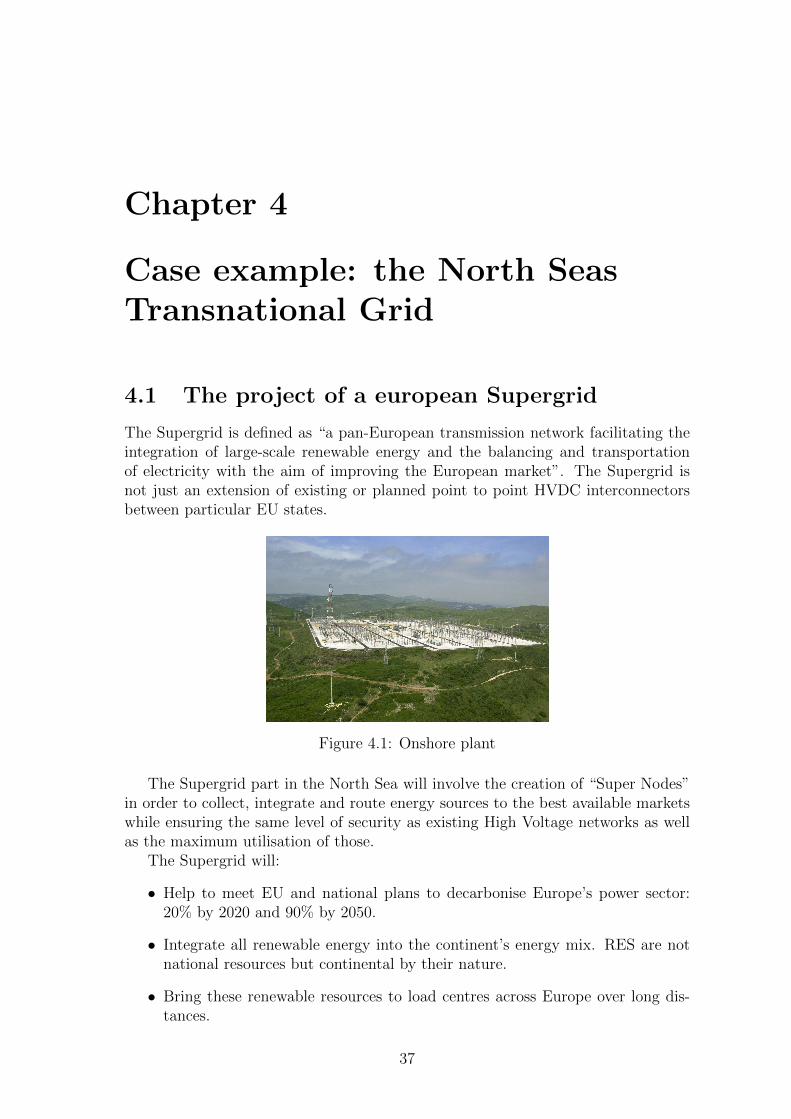
Figure 4.1: Onshore plant

The Supergrid part in the North Sea will involve the creation of “Super Nodes”in order to collect, integrate and route energy sources to the best available marketswhile ensuring the same level of security as existing High Voltage networks as wellas the maximum utilisation of those.

The Supergrid will:

• Help to meet EU and national plans to decarbonise Europe’s power sector:20% by 2020 and 90% by 2050.

• Integrate all renewable energy into the continent’s energy mix. RES are notnational resources but continental by their nature.

• Bring these renewable resources to load centres across Europe over long dis-tances.

37

4.2. The North Sea Transnational Grid Project 38

• Balance Europe’s electricity network and enhance security of supply.

• Create a global opportunity for European companies to export sustainableenergy technology and create new highly skilled jobs .

• Enhance the single European electricity market.

The concept of a european supergrid is fascinating and not to far from reality forwhat concerns technical aspects. In fact, the main issues facing the implementationof the grid are non-technical but legislative. The critical timeline for the introductionof new technology lies primarily in the solution of non-technical issues that will createa strong market growth and a technology push. An early solution of these hurdleswill influence the future roadmap to a greater extent than may be foreseen, due to theextended time constraints in planning and construction of new transmission capacity.As it is easy to imagine, many new norms should be produced by governments totutelate energy consumption and distribution and new organs should be createdto overcome this heavy work. Since any Country would pursue its own objectives,supergrid is something uthopistic: when the lack of fossil fuels becomes a realityEurope will be forced to make something similar to the supergrid happen.

4.2 The North Sea Transnational Grid Project

Besides the Supergrid, there is a smaller but not less ambitious project regardingthe North Sea area: The North Sea Transnational Grid Project (NSTGP).

The NSTGP, which will be taken as study case in this work, is a project involvingfive countries [18]. Its main objective is to determine the best solution (modular,flexible, most cost effective) for a high capacity transnational offshore grid, connect-ing all future wind farms in the northern part of the North Sea to the Netherlands,UK, Norway, Denmark and Germany. The NSTG project aims to identify and studytechnical and economic aspects with regard to the development of a transnationalelectricity network in the North Sea for the connection of offshore wind power andtrade between countries. The project is jointly executed by the Energy ResearchCentre of the Netherlands and the Delft University of Technology and it started inOctober 2009. The project is particuarly focused on:

• Determinating the optimal offshore grid configuration;

• Coordinating grid expansion plan;

• Evaluating the socio-economic consequences;

To achieve these objectives, the project is subdivided in the following specific sub-tasks:

- Inventory of available technologies;

- Technical and economic evaluation of different topology alternatives;

- Operation and control of a multi-terminal grid with different kinds of tech-nologies;

- Real-time multi-terminal converter simulation and testing;

4.3. Network Architecture 39

- Optimization of NSTG solutions

- Grid planning, congestion management, and stability evaluation;

- Costs, benefits, regulations, and market aspects of the NSTG and connectionalternatives;

The NSTG research project is coordinated by the Energy Research Centre of theNetherlands.

4.3 Network Architecture

Before describing the network topology that will be taken as study case by this work,the reasons of the need of a specific kind of structure are explained in the subsectionbelow.

4.3.1 System Design

It is very important to choose the most functional architeture from the beginningfor large scale projects such as the NSTG one. A possible definition of systemarchitecture is given by Ulrich [31]:

System architecture is the scheme by which the function of a system is allo-cated to physical components.

Therefore, system architecture can be seen as the way how components inside asystem interact and interface with each other [26]. There are two main types ofsystem architecture:

1. Integrated

2. Modular

An integrated designed system generally accomplishes to maximise a certain per-formance mesure but, on the other side, modifications to one feature or componentmay affect the whole system design. Observing the objectives of the NSTGP withinits complexity, it is easy to imagine that an integrated architecture would not be thebest solution to provide development and changes to the stations already built in thenorthern area: redesign the whole would be the only chance to adopt an integratedarchitecture. Hence, a modular solution seems to be the most suitable choice [18].Modularity can be seen as [5]:

The practice of building complex systems or processes from smaller subsys-tems that can be designed independently yet function together as a whole.

The main feature of a modular system is certainly that each module can be designedindependently, so this is the main reason why changes made in one module will notaffect the whole system.

As a modular project, the NSTG needs to set global design rules an local designrules, as shown in Fig. 4.2[26].


Figure 4.2: Design rules for the NSTG.

Before the development of such a complex system, system engineers should esta-bilish and take global designing rules into consideration. Proper development of thesystem global design rules can lead to dc grid code standards which could reducecosts by having a single common design, allowing systems to be built incrementallyand by different suppliers, thus supporting incremental investment plans. In thisway, a large pan-European offshore dc network would be developed “organically”.First by the construction of a few small independent dc grids with four to six ter-minals that, in a later stage, would be combined to form together a larger offshorenetwork with a more complex topology, such as a meshed multi-terminal dc network.Some stages of the possible evolution of the NTSG are shown in Fig. 4.3 [25].

4.3.2 Study Case

In order to study and test control strategies for Multi-terminal HVDC transmissionlines, a 19-node meshed grid, corresponding to the third evolution stage of theNSTG, has been taken as an example. The network architecture is shown in Fig.4.4 [30]

The network layout contains the five European countries with the highest ex-pected installed offshore capacity: UK, Denmark (DN), Germany (DE), Netherlands(NL), and Belgium (BE). It is made of 19 DC nodes and 19 DC transmission lineswhose parameters are displayed in Tab. 4.1.

Quantity ValueMaximum Power Pmax 150 MWMaximum Voltage Emax 150 kVCable resistance R 0.02Ω/km

Table 4.1: Essential network parameters.

In the example network, nodes are constituted by two types VSCs, denoted as:


(a) Phase 1. (b) Phase 2.

(c) Phase 3. (d) Phase 4.

Figure 4.3: NSTG possible evolution.

• Grid Side Converters (GSC): those placed on the mainland;

• Wind Farm Converters (WFC): those placed off-shore.

Grid side and wind farm nodes are described in Table 4.2.

Wind Farm Node Grid Side NodeDoggersbank UK1 England UKHornsea UK2 Belgium BEThortonbank BE1 Netherlands NLIjmuiden NL1 Germany DEEemshaven NL2 Denmark DKHochsee Sud DE1Hochsee Nord DE2Horns Rev DK1Ringcobing DK2

Table 4.2: WFCs description.

In this study case all the nodes are supposed to consume/produce their maximumpower. Moreover, since the network is heterogeneous, the agents are characterizedby having differents values of capacities and desired voltages as shown Tab. 4.3.


Figure 4.4: Study case.

Agent Type Capacity Ck Power Pmaxk Reference E∗k

UK1 WF 200 mF 140 MW 150 kVUK2 WF 100 mF 150 MW 150 kVUK GS 100 mF 100 MW 145 kVBE1 WF 140 mF 120 MW 150 kVBE GS 150 mF 100 MW 145 kVNL1 WF 150 mF 130 MW 150 kVNL2 WF 140 mF 140 MW 150 kVNL GS 200 mF 100 MW 145 kVDE1 WF 100 mF 130 MW 150 kVDE2 WF 200 mF 120 MW 150 kVDE GS 150 mF 100 MW 145 kVDK1 WF 140 mF 140 MW 150 kVDK2 WF 100 mF 140 MW 150 kVDK GS 150 mF 100 MW 145 kV

Table 4.3: Agents parameters.

Transmission lines lenght are given in Table 4.4.


Line Line Lenght ResistanceStart End [km] ΩUK1 HUB1 100 2.0UK2 HUB1 40 0.8UK HUB1 120 2.4HUB1 HUB2 300 6.0BE1 HUB2 50 1.0BE HUB2 100 2.0HUB2 HUB3 120 2.4NL1 HUB3 100 2.0NL2 HUB3 40 0.8NL HUB3 70 1.4HUB3 HUB4 250 5.0DE1 HUB4 40 0.8DE2 HUB4 70 1.4DE HUB4 150 3.0HUB4 HUB5 120 2.4DK1 HUB5 40 0.8DK2 HUB5 50 1.0DK HUB5 150 3.0HUB1 HUB5 380 7.6

Table 4.4: Network transmissions lenght.

In order to apply both Local and Global control strategies, there cannot be starnodes such as HUB1, HUB2, HUB3, HUB4 and HUB5 in the network. It is possibleto obtain an equivalent network without hubs using Rosen’s Theorem.

Ronsen’s Theorem and Equivalent Network

Given a network with star nodes, Rosen’s theorem allows to find a mesh equivalentnetwork where all the nodes are connected to each other. Rosen’s tranformation isgraphically shown in Fig. 4.5 [28].

Figure 4.5: Application of Rosen’s Theorem

Theorem 3 (Nodal-Mesh Transformation Theorem). For any network with N nodesconnected to a single node in a star fashion, with Y1,Y2,. . . ,YN being the conductances


of each branch, it is possible to find a mesh equivalent circuit where all the nodesare connected to each other, and with conduntances given by:

Ypq =YpYqN∑k=1

Yk

(4.1)

Therefore, from now on the network to be considered is shown in Fig. 4.6 and :

1. It is meshed (not nodal);

2. It has all the nodes connected to each other;

3. The equivalent conductances of the transmission lines have been obtained using(4.1).

A program that automatically calculates Rosen’s conductances has been writtenwith MATLAB and it is presented in the appendix.

Figure 4.6: Study case network.

Chapter 5

Local Control

In this chapter the main results about local control strategy for the network de-scribed in 4.3.2 are presented. The first section will be focused on the Droop Controltechnique, which is a classical control approach to HVDC transmission lines, whilethe second will be about Droop control, in fact a proportional control, plus integraland derivative actions.

5.1 Droop Control

The idea of the Droop Control strategy is to achieve DC voltage regulation usinga decentralized approach, designed to allow proper transmission of the generatedpower from the WFCs to the GSCs, while maintaining the voltage of the HVDC ina safe range of operation [1]. The droop controller is a proportional control law, thatregulates the DC voltage and provides power sharing between the different powerconverters [10]. The conventional droop controller is a heuristic based on physicalintuition gleaned from the study of high voltage Wide Area Electric Power System(WAEPS), and at its core relies on the decoupling of active and reactive power forsmall power angles and non-mixed line conditions [27].

Droop control consists in a nonlinear static relationship between the currentprovided by the VSC, Ik, and the voltage across each capacitor, Ek [6]. Its objectiveis to maintain the characteristic ΦE

k := (Ek, I(Ek)) inside an admissibility regionwhich depends on the nature of the node, as can be seen in Fig. 5.1. The grey zonerepresents the admissibility region while the blue and red curves represent its limitsand also the desired working mode to maximize power exploitation.

Droop control can be seen as an algorithm such as:

Ik =

Imaxk if Ek ≤ PkI/I

maxk

PkI

Ekif PkI/I

maxk < Ek < El

k

−mdk(Ek − E∗k) if El

k < Ek < Ehk

PkC

Ekif El

k < Ek

(5.1)

Let us define the entites in (5.1):

• Imaxk is the maximum current that is able to flow trough the node k. It is the

same for all the VSCs and it is equal to 1kA.

• −mdk is the control proportional gain.

45

5.1. Droop Control 46

Figure 5.1: Droop Control Curves [6]

• PkI is the power injected by the k-th WFC.

• PkC is the power consumed by the k-th GSC.

• Elk is the lower limit of the droop zone for the node k.

• Ehk is the higher limit of the droop zone for the node k.

• Ek is the voltage of the node k.

Elk and Eh

k define the droop operational mode dimension. In fact, a network canoperate in:

1. Normal operation mode: when the characteristic ΦEk := (Ek, I(Ek)) belongs

to the semi-hyperbolic region, as can be seen in Fig. 5.1.

2. Droop operation mode: when the characteristic ΦEk := (Ek, I(Ek)) follows the

straight line with slope −mdk and the droop control is active.

Elk and Eh

k can be obtained as [6]:

Elk =

1

2

(E∗k +

√(E∗k)2 − 4

PkI

mk

)(5.2)

Ehk =

1

2

(E∗k +

√(E∗k)2 − 4

PkC

mk

)(5.3)

It is important to notice that the power is assumed to be:

• PkC = −Pmaxk for the GSCs;

• PkI = Pmaxk for the WFCs.

Moreover the consumed power is assumed to be 0 for the WFCs so their Ehk

coincides with E∗k .

5.2. PID Droop Control 47

Simulations

The system described in section 4.3.2 has been simulated using MATLAB/Simulink.The first simulation refers to the system in regularl conditions, with constant powerPmax as defined in last section. The results can be seen in Fig. 5.2.

0 1 2 3 4 5 6 7 8 9 101.455

1.46

1.465

1.47

1.475

1.48

1.485

1.49

1.495

1.5x 10

5

t[s]

volta

ge[V

]

(a) Voltages.

0 1 2 3 4 5 6 7 8 9 10−800

−600

−400

−200

0

200

400

600

800

1000

t[s]

curr

ent[A

]

(b) Capacitors Currents.

0 1 2 3 4 5 6 7 8 9 10−5000

−4000

−3000

−2000

−1000

0

1000

2000

3000

4000

5000

t[s]

erro

r[V

]

(c) Error.

Figure 5.2: Droop control: regular operation

In the second simulation at t = 20s the power Pmax decreases by ten times. It ispossible to see in Fig. 5.3 and 5.2, that in both cases stability is preserved and bothvoltages and currents remain in the admissibility region. This is shown in Fig. 5.4for two WFCs, UK1 and DK1, and two GSCs, UK and DK: voltages, powers andcurents is maintained into the admissibility region.

5.2 PID Droop Control

The PID droop control strategy replaces the conventional droop law (5.1) by:

Ik = −mdk(Ek(t)− E∗k)− β

∫(Ek(t)− E∗k)dt− γ ˙(Ek(t)− E∗k), (5.4)

with the necessary saturation in order to keep the system within the admissibilityregion. When integral and derivative actions are added, it is not possible to consider


0 5 10 15 20 25 30 35 401.455

1.46

1.465

1.47

1.475

1.48

1.485

1.49

1.495

1.5x 10

5

t[s]

volta

ge[V

]

(a) Voltages.

0 5 10 15 20 25 30 35 40−800

−600

−400

−200

0

200

400

600

800

1000

t[s]

curr

ent[A

]


0 5 10 15 20 25 30 35 40−5000

−4000

−3000

−2000

−1000

0

1000

2000

3000

4000

5000

t[s]

erro

r[V

]

(c) Error.

Figure 5.3: Droop control: power decrease at t = 20s

the same saturation used in the previous section because Elk and Eh

k depend only onthe proportional gain. Therefore, to be able to employ the integral action, a currentsaturation like the one in Fig. 5.5 has been used.

Figure 5.5: PI droop control: implementation procedure

As can be seen in Fig. 5.5, the control block produces the current Ik, whichwould be needed to make the error tend to zero. Multiplying it out by the actualnetwork voltage Ek, one gets the required power, Pk. Since the control objectiveis to maintain currents and voltages in the admissibility region, and the network isnot able to provide more than 200 MW, a power saturation is employed to avoid an


0 2 4 6 8 10 12 14 16 18 200

500

1000

curr

ent

0 2 4 6 8 10 12 14 16 18 201.46

1.47

1.48

1.49

1.5x 10

5

volta

ge

0 2 4 6 8 10 12 14 16 18 200

5

10

15x 10

7

pow

er

(a) UK1.

0 2 4 6 8 10 12 14 16 18 200

500

1000

curr

ent

0 2 4 6 8 10 12 14 16 18 201.46

1.47

1.48

1.49

1.5x 10

5

volta

ge

0 2 4 6 8 10 12 14 16 18 200

5

10

15x 10

7

pow

er

(b) DK1.

0 2 4 6 8 10 12 14 16 18 20−1000

−500

0

curr

ent

0 2 4 6 8 10 12 14 16 18 201.4

1.45

1.5

1.55x 10

5

volta

ge

0 2 4 6 8 10 12 14 16 18 20−1

−0.5

0

0.5

1x 10

8

pow

er

(c) UK.

0 2 4 6 8 10 12 14 16 18 20−1000

−500

0

curr

ent

0 2 4 6 8 10 12 14 16 18 201.4

1.45

1.5

1.55x 10

5vo

ltage

0 2 4 6 8 10 12 14 16 18 20−5

0

5

10x 10

7

pow

er

(d) DK.

Figure 5.4: Droop control under regular operation: evolution of the curves withinthe admissibility region.

excessive power flow. After this step, dividing the real power, P rk , obtained by means

of saturation, by the voltage Ek, one calculates the real control current, Irk , that canflow through the network without causing an excessive power flow. However, as Irkcould be higher than Imax or lower than Imin, a current saturation is applied toobtain the current actually delivered to the system, Ifk .

Simulations

The first simulation, shown in Fig. 5.6, has been made using an integral gain β = md

which is 0.25 for the WFCs and 0.20 for the GSCs and γ = 0. In order to see howthe system reacts when β tends to one, the second simulation has been made varyingthe integral gain as can be seen in Fig. 5.7. Considering Table 5.1, it is possible tonotice that, as the gain grows the system dynamics is faster and the error decreasesbut there is a visible current overshoot which means an higher control effort.

Adding a derivative action with gain γ = 0.1 and setting β = 0.6, the systemdynamics is shown in Fig. 5.8.

According to Fig. 5.9 it is possible to say that the derivative action does not bringany improvement to the system behaviour, in fact, the dynamics becomes a littleslower and a small undershoot appears without any consistent error reduction. All

5.3. Conclusions and Comparisons 50

0 1 2 3 4 5 6 7 8 9 101.44

1.45

1.46

1.47

1.48

1.49

1.5

1.51x 10

5

t[s]

volta

ge[V

]

(a) Voltages.

0 1 2 3 4 5 6 7 8 9 10

−1000

−800

−600

−400

−200

0

200

400

600

800

1000

t[s]

curr

ent[A

]


0 1 2 3 4 5 6 7 8 9 10−2.5

−2

−1.5

−1

−0.5

0

0.5

1

1.5

2

2.5x 10

8

t[s]

pow

er[W

]

(c) Power.

0 1 2 3 4 5 6 7 8 9 10−5000

−4000

−3000

−2000

−1000

0

1000

2000

3000

4000

5000

t[s]

erro

r[V

]

(d) Error.

Figure 5.6: PI droop control under regular operation

the previous versions have proved to be stable and evolving within the admissibilityregion. Fig. 5.10 shows this feature to the nodes UK1, DK1, UK and DK evolveinside their admissibility region.

5.3 Conclusions and Comparisons

To conclude, a comparison between the two control techniques described in theprevious sections is given. Since the derivative action does not provide any significantimprovement, the comparison will be made considering the traditional Droop controllaw and the PI control law, obtained considering (5.4) with γ = 0.

The first comparison shows the differences between the two strategies when thenetwork is operating with constant power flow, the results can be seen in Fig. 5.11.The most relevant thing is that the Droop currents are in average lower than PIcurrents, so the required control effort is lower in the first case. Neverthless, asFig. 5.11(e),(f) show, more nodes are able to reach exactly their reference with PIcontrol and, the error is generally lower in this case.

The second comparison has been made considering a power reduction of ten timesPmax, Fig. 5.12. It is clear that the network controlled by simple Droop reacts better


β = 0.3 β = 0.6 β = 0.910−4×-0.0531 -0.0518 -0.0507-0.0753 -0.0739 -0.07280.8493 0.8476 0.8467-0.0005 -0.0001 0.00050.8357 0.8341 0.8332-0.0059 -0.0015 0.00010.0015 -0.0005 0.00030.7101 0.7092 0.70850.0016 -0.0004 0.00030.0027 -0.0006 0.00040.1874 0.1892 0.18920.0008 -0.0003 0.00020.0007 -0.0002 0.00010.0006 0.0000 -0.0000

Table 5.1: Squared 2-norm error.

to this kind of disturbance. In fact, the reaction is almost instantaneous while, in PIcontrol case, the system takes around ten seconds to reach the equilibrium again.


0 1 2 3 4 5 6 7 8 9 101.44

1.45

1.46

1.47

1.48

1.49

1.5

1.51x 10

5

(a) Voltages with β = 0.3.

0 1 2 3 4 5 6 7 8 9 10

−1000

−800

−600

−400

−200

0

200

400

600

800

1000

(b) Currents with β = 0.3.

0 1 2 3 4 5 6 7 8 9 101.44

1.45

1.46

1.47

1.48

1.49

1.5

1.51x 10

5

(c) Voltages with β = 0.6.

0 1 2 3 4 5 6 7 8 9 10

−1000

−800

−600

−400

−200

0

200

400

600

800

1000

(d) Currents with β = 0.6.

0 1 2 3 4 5 6 7 8 9 101.44

1.45

1.46

1.47

1.48

1.49

1.5

1.51

1.52x 10

5

(e) Voltages with β = 0.9.

0 1 2 3 4 5 6 7 8 9 10

−1000

−800

−600

−400

−200

0

200

400

600

800

1000

(f) Currents with β = 0.9.

Figure 5.7: PI droop control regular operation: dynamics with different values of β


0 5 10 151.44

1.45

1.46

1.47

1.48

1.49

1.5

1.51x 10

5

t[s]

volta

ge[V

]

(a) Voltages.

0 1 2 3 4 5 6 7 8 9 10

−1000

−800

−600

−400

−200

0

200

400

600

800

1000

t[s]

capa

cito

rs c

urre

nt[A

]


0 1 2 3 4 5 6 7 8 9 10−2.5

−2

−1.5

−1

−0.5

0

0.5

1

1.5

2

2.5x 10

8

t[s]

pow

er[W

]

(c) Power.

0 5 10 15−5000

−4000

−3000

−2000

−1000

0

1000

2000

3000

4000

5000

t[s]

erro

r[V

]

(d) Error.

Figure 5.8: PID droop control regular operation


0 5 10 151.44

1.45

1.46

1.47

1.48

1.49

1.5

1.51x 10

5

(a) Voltages with PI

0 5 10 151.44

1.45

1.46

1.47

1.48

1.49

1.5

1.51x 10

5

(b) Voltages with PID

0 1 2 3 4 5 6 7 8 9 10

−1000

−800

−600

−400

−200

0

200

400

600

800

1000

(c) Currents with PI

0 1 2 3 4 5 6 7 8 9 10

−1000

−800

−600

−400

−200

0

200

400

600

800

1000

(d) Currents with PID.

0 5 10 15−5000

−4000

−3000

−2000

−1000

0

1000

2000

3000

4000

5000

(e) Errors with PI

0 5 10 15−5000

−4000

−3000

−2000

−1000

0

1000

2000

3000

4000

5000

(f) Errors with PID

Figure 5.9: PID droop control: comparison between PI and PID


0 2 4 6 8 10 12 14 16 18 200

500

1000

curr

ent

0 2 4 6 8 10 12 14 16 18 201.46

1.48

1.5

1.52x 10

5

volta

ge

0 2 4 6 8 10 12 14 16 18 200

0.5

1

1.5

2x 10

8

pow

er

(a) UK1.

0 2 4 6 8 10 12 14 16 18 200

500

1000

curr

ent

0 2 4 6 8 10 12 14 16 18 201.46

1.48

1.5

1.52x 10

5

volta

ge

0 2 4 6 8 10 12 14 16 18 200

5

10

15x 10

7

pow

er

(b) DK1.

0 2 4 6 8 10 12 14 16 18 20−1000

−500

0

curr

ent

0 2 4 6 8 10 12 14 16 18 201.4

1.45

1.5

1.55x 10

5

volta

ge

0 2 4 6 8 10 12 14 16 18 20−2

−1

0

1x 10

8

pow

er

(c) UK.

0 2 4 6 8 10 12 14 16 18 20−1000

−500

0

curr

ent

0 2 4 6 8 10 12 14 16 18 201.4

1.45

1.5

1.55x 10

5

volta

ge

0 2 4 6 8 10 12 14 16 18 20−1

−0.5

0

0.5

1x 10

8

pow

er

(d) DK.

Figure 5.10: PID droop control: evolution of the curves within the admissibilityregion


0 1 2 3 4 5 6 7 8 9 101.455

1.46

1.465

1.47

1.475

1.48

1.485

1.49

1.495

1.5x 10

5

t[s]

volta

ge[V

]

(a) Voltages with Droop

0 1 2 3 4 5 6 7 8 9 101.44

1.45

1.46

1.47

1.48

1.49

1.5

1.51x 10

5

t[s]

volta

ge[V

](b) Voltages with PI Droop

0 1 2 3 4 5 6 7 8 9 10−800

−600

−400

−200

0

200

400

600

800

1000

t[s]

curr

ent[A

]

(c) Currents with Droop

0 1 2 3 4 5 6 7 8 9 10

−1000

−800

−600

−400

−200

0

200

400

600

800

1000

t[s]

curr

ent[A

]

(d) Currents with PI Droop.

0 1 2 3 4 5 6 7 8 9 10−5000

−4000

−3000

−2000

−1000

0

1000

2000

3000

4000

5000

t[s]

erro

r[V

]

(e) Errors with Droop

0 1 2 3 4 5 6 7 8 9 10−5000

−4000

−3000

−2000

−1000

0

1000

2000

3000

4000

5000

t[s]

erro

r[V

]

(f) Errors with PI Droop

Figure 5.11: PI droop and Droop control regular operation comparison


0 5 10 15 20 25 30 35 401.455

1.46

1.465

1.47

1.475

1.48

1.485

1.49

1.495

1.5x 10

5

t[s]

volta

ge[V

]

(a) Droop Voltages

0 5 10 15 20 25 30 35 401.32

1.34

1.36

1.38

1.4

1.42

1.44

1.46

1.48

1.5

1.52x 10

5

(b) PI Droop voltages

0 5 10 15 20 25 30 35 40−5000

−4000

−3000

−2000

−1000

0

1000

2000

3000

4000

5000

t[s]

erro

r[V

]

(c) Droop Errors

0 5 10 15 20 25 30 35 40−1.5

−1

−0.5

0

0.5

1x 10

4

(d) PI Droop Errors

Figure 5.12: PI droop and Droop control: power decrease comparison

Chapter 6

Global Control

This chapter is about a Global control technique. The term global is due to the factthat the implemented control law acts on the entire network to set the referenceerror to zero: a consensus strategy is employed to make voltages follow a constantreference. The idea is to consider the error model form (3.9) of the system given inFig. 4.6 and make it reach consensus to zero. The control strategies used in thischapter are adapt those presented in [9] for generic networks.

6.1 Global PID Control

The main objective of this control strategy is to regulate the voltages to the set-point values E∗, given in Table 4.3. The control laws will be tested on the studycase (heterogeneous) network, and also on an homogeneous version of it. The net-work parameters for the heterogeneous case are the ones in Table 4.3 while forthe homogeneous case the only difference is that the capacities are assumed to beC1 = C2 = · · · = CN = 200mF , which means that all the VSCs are equal. Asanticipated before, the regulation will be obtained by means of consensus technique.In particular, this section will refer to admissible consensus.

Definition 13 (Admissible Consensus). A network is said to reach admissible con-sensus if, for any set of initial conditions:

limt→∞

xi(t) ∈ C, |ui(t)| < +∞ ∀t ≥ 0, i ∈ N , (6.1)

where C is the Consensus Manifold. Moreover, if:

limt→∞‖xj(t)− xi(t)| ≤ ε for ε > 0, (6.2)

the network is said to achieve ε−admissible consensus.

6.1.1 A different Model

In order to apply Global PID Control (GPIDC) , the system must be in the form:

xi(t) = ρixi(t) + δi + ui(t), i ∈ N, (6.3)

where:

58

6.1. Global PID Control 59

• xi(t) is the state of the i-th agent

• ρi ∈ R is the agent pole determing its uncoupled dynamics

• δi ∈ R is some constant disturbance

• ui(t) ∈ R is the global control input

The desired control law is a PID in the form:

ui(t) = −N∑j=1

Gij

(αxj(t) + β

∫ t

0

xj(τ)dτ + γxj(t)

), (6.4)

in which:

• Gij are elements of the Laplacian matrix

• α, β, γ are respectively the Proportional, Integral and Derivative gains.

To apply the desired control law, the HVDC network model:

CiEi = Ii(Ei) +N∑j=1

aij1

Rij

(Ej − Ei), (6.5)

must be brought into the generic form (6.3), passing through the error formulationas in (3.7). Defining:

δ = −GE∗, (6.6)

rewriting the control law in matrix form:

u = −αGe− βG

∫e− γGe, (6.7)

setting the current as:

I(e) = Pe− αGe− βG

∫e− γGe, (6.8)

where P is the diagonal matrix of the poles, and finally substituting in the originalnetwork model (3.9), the resulting model:

Ce = Pe + u + δ, (6.9)

where:

u = −(1 + α)Ge− βG

∫e− γGe. (6.10)

finally matches (6.3).It is now possible to compare the Local PID control law (5.4), with (6.8). It

can be seen that the first one, being local, takes into account single node dynamics:Ik = Ik(ek). The second is a global control law and, in fact, the current suppliedto the k-th node depens not only on ek but on e and on the topology, that isIk = Ik(e,G).

Before moving forward to the control results, it is important to notice a propertyof δ.

6.2. Homogeneous Network 60

Theorem 4 (Property of δ). The sum of all the components of the disturbancevector delta defined in (6.6) is zero, i.e.

N∑k=1

δk = 0 (6.11)

Proof. Using (6.6) one has that:

N∑k=1

δk =

((1 1 1 1

)G

E∗1E∗2E∗3E∗4

)T

=(E∗1 E∗2 E∗3 E∗4

)G

1111

= 0, (6.12)

The last equality follows from the fact that G is a laplacian and, therefore, (1, . . . , 1)T

is an eigenvector of eigenvalue 0.

6.2 Homogeneous Network

In this section theoretical results and simulations regarding the network model builtassuming identical converters will be given. The homogeneous network model isobtained by assuming capacities and poles to be the same for each VSC.

PID strategy

Theorem 5 (PID (homogeneous) strategy). The closed-loop network (6.9) withρi = ρj = −ρ∗, ρ∗ ∈ R+ for i, j ∈ 1, ..., N achieves admissible consensus for anypositive value of α, β and γ. All node states converge to:

e∞ = (1/N)N∑k=1

δk/ρ∗, (6.13)

and the integral action norm is limited by:

z∞ ≤√N3(N − 1)

γλ2 + 1||δ||, (6.14)

with z = −βG∫e.

Since e∞ is defined as (6.13), due to Theorem 4 it is always zero. This is whyconsidering the system in the error state form and applying consensus theory, it ispossible to achieve a perfect voltage regulation. The simulation results are shownin Fig. 6.1


0 5 10 15 20 25 301.44

1.45

1.46

1.47

1.48

1.49

1.5

1.51x 10

5

t[s]

volta

ge[V

]

(a) Voltages

0 5 10 15 20 25 30−8

−6

−4

−2

0

2

4

6

8

10x 10

9

t[s]

curr

ent[A

]

(b) Currents

0 5 10 15 20 25 30−5

−4

−3

−2

−1

0

1

2

3x 10

8

t[s]

z

(c) Integral Actions

0 5 10 15 20 25 30−5000

−4000

−3000

−2000

−1000

0

1000

2000

3000

4000

5000

t[s]

erro

r[V

]

(d) Errors

Figure 6.1: PID Homogeneous Control with α = 25, β = 5, γ = 6

PI strategy

Theorem 6 (PI (homogeneous) strategy). Under the action of the global proportional-integral (PI) control obtained by setting γ = 0 in (6.10), an homogeneous network ofN linear systems in the form (6.9), achieves admissible consensus for any positivevalue of α and β. All node states converge to (6.13) and the integral action norm islimited by:

z∞ ≤√N(N − 1)||δ|| (6.15)

The simulation obtained with PI strategy are shown in Fig. 6.2.


0 5 10 15 20 25 301.44

1.45

1.46

1.47

1.48

1.49

1.5

1.51

1.52x 10

5

t[s]

volta

ge[V

]

(a) Voltages

0 5 10 15 20 25 30−1

−0.8

−0.6

−0.4

−0.2

0

0.2

0.4

0.6

0.8

1x 10

8

t[s]

curr

ent[A

]

(b) Currents

0 5 10 15 20 25 30−2

−1.5

−1

−0.5

0

0.5

1

1.5

2x 10

8

t[s]

z


0 5 10 15 20 25 30−5000

−4000

−3000

−2000

−1000

0

1000

2000

3000

4000

5000

t[s]

erro

r[V

]

(d) Errors

Figure 6.2: PI Homogeneous Control α = 25, β = 5

It is possible to say, comparing Fig. 6.1 and Fig. 6.2, that without the derivativeaction the system is faster but much less smooth. An important characteristic of PIstrategy is that it guarantees that all the nodes converge to the same asymptoticvalue despite the presence of disturbances. Although, consensus is reached at a valuethat depends on disturbance amplitude, as can be seen in Fig. 6.3, where a stepdisturbance has been added to δ at t = 15s.

0 5 10 15 20 25 30−6000

−4000

−2000

0

2000

4000

6000

8000

t[s]

erro

r[V

]

(a) Errors with disturbance ampli-tude=20000

0 5 10 15 20 25 30−5000

0

5000

10000

15000

20000

t[s]

erro

r[V

]

(b) Errors with disturbance ampli-tude=50000

Figure 6.3: Network reaction to disturbances whith PI control


PD strategy

Theorem 7 (PD (homogeneous) strategy). The network with homogeneous nodedynamics in the form (6.9), controlled by the distributed PD control obtained byselecting α > 0, β = 0, γ > 0 in (6.10), achieves ε-admissible consensus with:

ε =γλN + 1

γλ2 + 1

N

αλN + ρ∗||δ|| (6.16)

In fact, as shown in Fig. 6.4, whithout the integral action, the network is notable to reach perfect consensus and a little error still remains.

0 5 10 15 20 25 301.45

1.46

1.47

1.48

1.49

1.5

1.51x 10

5

t[s]

volta

ge[V

]

(a) Voltages

0 5 10 15 20 25 30−1

−0.8

−0.6

−0.4

−0.2

0

0.2

0.4

0.6

0.8

1x 10

8

t[s]

curr

ent[A

]

(b) Currents

0 5 10 15 20 25 30−5000

−4000

−3000

−2000

−1000

0

1000

2000

3000

4000

5000

t[s]

erro

r[V

]

(c) Errors

Figure 6.4: PD Homogeneous Control α = 25, β = 0,γ = 6

Moreover, since ε depends from α, increasing it will make the stady-state errordecrease, as depicted in Fig. 6.5.

6.3. Heterogeneous Network 64

0 5 10 15 20 25 30−5000

−4000

−3000

−2000

−1000

0

1000

2000

3000

4000

5000

t[s]

erro

r[V

]

(a) Errors with α = 25

0 5 10 15 20 25 30−5000

−4000

−3000

−2000

−1000

0

1000

2000

3000

4000

5000

t[s]

erro

r[V

]

(b) Errors with α = 100

Figure 6.5: PD Homogeneous Control with different α, β = 0,γ = 6

6.3 Heterogeneous Network

In this section the network parameters to be considered are the ones in Table.4.3. The nodes are characterized by having different capacities and different poles,therefore, this is the case of the North Sea Transnational Grid.

PID strategy

Theorem 8 (PID (heterogeneous) strategy). The heterogeneous group of agentscontrolled by the global PID strategy, achieves admissible consensus for any β > 0and γ ≥ 0, if the following conditions hold:

1.

ψ = (1/N)N∑k=1

ρk < 0 (6.17)

2.

α >γλ2 + 1

2λ2

(|||H1|||2

2Nκ

ρρT

|ψ|+ |||H2|||

)(6.18)

where:H1 := IN−1 + H, (6.19)

andH2 := H(P + ρ11N−11

TN−1) + (P + ρ11N−11

TN−1)H

T , (6.20)

with IN−1 identity matrix, P = [ρ2, . . . , ρN ], ρi i-th pole, 1N−1 = (N − 1)× 1vector of 1.1

Moreover, all the nodes states converge to e∞ and the integral action is limted by:

z∞ ≤√N(N − 1)||H||

(1 +

||ρ||N |ψ|

)||δ||, (6.21)

where:ρ = [ρ2 − ρ1, . . . , ρN − ρ1]. (6.22)

1The calculation of H is explicited in the appendix.


This case simulations are shown in Fig. 6.6.

0 5 10 15 20 25 301.44

1.45

1.46

1.47

1.48

1.49

1.5

1.51

1.52x 10

5

t[s]

volta

ge[V

]

(a) Voltages

0 5 10 15 20 25 30−1

−0.8

−0.6

−0.4

−0.2

0

0.2

0.4

0.6

0.8

1x 10

8

t[s]

curr

ent[A

]

(b) Currents

0 100 200 300 400 500 600 700 800 900 1000−2

−1.5

−1

−0.5

0

0.5

1

1.5

2x 10

8

t[s]

z


0 5 10 15 20 25 30−5000

−4000

−3000

−2000

−1000

0

1000

2000

3000

4000

5000

t[s]

erro

r[V

]

(d) Errors

Figure 6.6: PID Heterogeneous Control α = αmin = 720, β = 5,γ = 0.6

It is now interesting to carry out a comparison between PID and PI on theheterogeneous network. As can be seen in Fig. 6.7, the dynamics of the system withγ = 0 is faster than the other, but it is also true that, since the delay is really small,a lighter stress for the cables can be welcomed. Adding a 200V step disturbance inthe action line, the reaction of the system is shown in Fig. 6.9. Making a zoom onthe error it is possible to notice that the network PI controlled is able to reject thedisturbance as good as the other one.

6.4 Conclusions and Comparisons

To make a comparison between homogeneous and heterogeneous dynamics, it ispossible to say, as can be seen in Fig. 6.10, that in the first case the system isfast, in fact it reaches perfect consensus in a very short amount of time. Regardingthe heterogeneous case, instead, low values of the error are obtained quickly butthe integral action continues to grow until the value zero is reached. It is worthremarking that for the global control strategies the system was not required toevolve within an admissibility region, that is, no bounds were assumed for powersand curents. An attempt to use the current saturation procedure used for thelocal PID droop control described in Section 5.2 yielded unstable behaviors. Theaddressing of this issue is left for further research.


0 0.2 0.4 0.6 0.8 1 1.2 1.4 1.6 1.8 21.44

1.45

1.46

1.47

1.48

1.49

1.5

1.51

1.52x 10

5

t[s]

volta

ge[V

]

(a) Voltages PID

0 0.2 0.4 0.6 0.8 1 1.2 1.4 1.6 1.8 21.44

1.45

1.46

1.47

1.48

1.49

1.5

1.51

1.52x 10

5

t[s]

volta

ge[V

]

(b) Voltages PI

0 0.2 0.4 0.6 0.8 1 1.2 1.4 1.6 1.8 2−5000

−4000

−3000

−2000

−1000

0

1000

2000

3000

4000

5000

t[s]

erro

r[V

]

(c) Errors PID

0 0.2 0.4 0.6 0.8 1 1.2 1.4 1.6 1.8 2−5000

−4000

−3000

−2000

−1000

0

1000

2000

3000

4000

5000

t[s]

erro

r[V

]

(d) Errors PI

Figure 6.7: PID and PI Heterogeneous Control comparison, α = 920, β = 5,γ = 10or γ = 0


0 0.2 0.4 0.6 0.8 1 1.2 1.4 1.6 1.8 21.44

1.45

1.46

1.47

1.48

1.49

1.5

1.51

1.52x 10

5

t[s]

volta

ge[V

]

(a) Voltages PID

0 0.2 0.4 0.6 0.8 1 1.2 1.4 1.6 1.8 21.44

1.45

1.46

1.47

1.48

1.49

1.5

1.51

1.52x 10

5

t[s]

volta

ge[V

]

(b) Voltages PI

0 0.2 0.4 0.6 0.8 1 1.2 1.4 1.6 1.8 2−5000

−4000

−3000

−2000

−1000

0

1000

2000

3000

4000

5000

t[s]

erro

r[V

]

(c) Errors PID

0 0.2 0.4 0.6 0.8 1 1.2 1.4 1.6 1.8 2−5000

−4000

−3000

−2000

−1000

0

1000

2000

3000

4000

5000

t[s]

erro

r[V

]

(d) Errors PI

Figure 6.8: PID and PI Heterogeneous Control comparison, disturbance reaction

0.8 0.9 1 1.1 1.2 1.3 1.4 1.5 1.6 1.7 1.8−20

0

20

40

60

80

100

120

140

160

180

200

t[s]

erro

r[V

]

(a) Errors PID

0.8 0.9 1 1.1 1.2 1.3 1.4 1.5 1.6 1.7 1.8−20

0

20

40

60

80

100

120

140

160

180

200

t[s]

erro

r[V

]

(b) Errors PI

Figure 6.9: PID and PI Heterogeneous Control comparison, disturbance reaction


0 5 10 15 20 25 30−1

−0.8

−0.6

−0.4

−0.2

0

0.2

0.4

0.6

0.8

1x 10

9

t[s]

curr

ent[A

]

(a) Currents PID Homo.

0 5 10 15 20 25 30−1

−0.8

−0.6

−0.4

−0.2

0

0.2

0.4

0.6

0.8

1x 10

9

t[s]

curr

ent[A

](b) Currents PID Hetero.

0 5 10 15 20 25 30−5

−4

−3

−2

−1

0

1

2

3x 10

8

t[s]

z

(c) Integral Acion PID Homo.

0 50 100 150 200 250 300 350−2

−1.5

−1

−0.5

0

0.5

1

1.5x 10

8

t[s]

z

(d) Integral Action PID Hetero.

0 5 10 15 20 25 30−5000

−4000

−3000

−2000

−1000

0

1000

2000

3000

4000

5000

t[s]

erro

r[V

]

(e) Errors PID Homo.

0 5 10 15 20 25 30−5000

−4000

−3000

−2000

−1000

0

1000

2000

3000

4000

5000

t[s]

erro

r[V

]

(f) Errors PID Hetero.

Figure 6.10: PID Homogeneous and Heterogeneous Case Comparison.

Chapter 7

Conclusions

7.1 Comparison between Local and Global Con-

trol

Before comparing the control strategies described in chapters 5, 6, let us rememberthat thay have different objectives:

• The aim of the Local Control is to maintain voltages and currents into anadmissibility region so that the network does not suffer an excessive amountof power flow;

• The goal of the Global Control is to make voltages perfectly follow a constantreference.

Hence, it is possible to say that control strategy should be chosen regarding theneeds of the network and mostly on the middle and upper level controllers. Forinstance: if the middle level controller is structured to optimize voltages values, itcan be wiser to chose global control so that there is no need to rebuild the wholecontrol architecture; otherwise, if it is oriented to produce the optimal curve as inFig. 5.1, it could be better to go for the local control technique.

Moreover, a relevant comparison can be made about the control effort. Since inboth control strategies the current is used to control voltages, it is possible to seein Fig. 7.1 that the global control effort is much higher than the local one. Such ahigh current may not always be available or sustainable, so perfect consensus maycome at a high price or even be unreacheable in a realistic system. On the otherhand, local control cannot garantee that the error goes to zero for each node but,as discussed in chapter 5, this is accetable since the network is protected from toohigh values of voltage and power.

Therefore, to conclude it is possible to say that local control strategy representsa better compromise between results and control effort than the global one, but, ifprecise values of voltage are requested, the global control technique provides betterperformances.

7.2 Future Work

The complex network approach discussed in this thesis, is the first of many possiblefuture works to improve the control of power networks. Possible fields of study can

69


0 1 2 3 4 5 6 7 8 9 10

−1000

−800

−600

−400

−200

0

200

400

600

800

1000

t[s]

capa

cito

rs c

urre

nt[A

]

(a) Currents PID Droop

0 1 2 3 4 5 6 7 8 9 10−1

−0.8

−0.6

−0.4

−0.2

0

0.2

0.4

0.6

0.8

1x 10

8

t[s]

curr

ent[A

]

(b) Currents PID Heterogeneous Global

Figure 7.1: Control Effort Comparison.

be the following:

• Studying the stability conditions;

• Testing the obtained results on a physical system;

• Investigating a possible hybrid system, where a complex network approachon the producing nodes can coexist with a different control strategy on theconsuming nodes;

• Formalizing and extending upper and middle level complex networks-basedcontrol techniques;

• Studying how much different topologies influence control performance;

• Adding a saturation in the Global PID control.

Bibliography

[1] A. Junyent-Ferre G. Gross O. Gomis-Bellmunt A. Egea-Alvarez F. Bianchi.“Voltage Control of Multiterminal VSC-HVDC Trasmission Systems for Off-shore Wind Power Plants: Design and Implementation in a Scaled Platform”.In: IEEE Transactions on Industrial Electronics (2013).

[2] International Energy Agency. World Energy Outlook. Paris: IEA, 2012.

[3] R. Albert I. Albert and G. Nakarado. “Structural vulnerability of the northamerican power grid”. In: Physical Review E vol. 69.4 (2004).

[4] Massoud Amin. MRS Bullettin-Harnessing materials for energy. 2008.

[5] C. Baldwin and K. Clark. Design Rules: The power of modularity. Massachusetts:MIT Press, 2000.

[6] A. Doria-Cerezo J.M. Olm M. di Bernardo M. Quaglia E. Nuno. “Bounded syn-chronization in resistive multi-terminal VSC-HVDC transmission systems”. In:IEEE (2014).

[7] A. Bodin. “HVDC light a preferable power transmission system for renewableenergies”. In: Proc. 3rd IYCE (2011).

[8] N. Mahimkar G. Persson C.Westerlind. “HVDC Technology for Large ScaleOffshore Wind Connections”. In: Proc. at Smartelec (2013).

[9] M. di Bernardo D. Burbano. “Distributed PID Control for Consensus of Ho-mogeneous and Heterogeneous Networks”. In: IEEE (2014).

[10] O. Gomis-Bellmunt F. D. Bianchi. “Droop control design for multi-terminalVSC- HVDC grids based on LMI optimization”. In: Proc. 50th Conf. Deci-sional Control (2011).

[11] O. Gomis-Bellmunt. “Topologies of multiterminal HVDC-VSC transmissionfor large offshore wind farms”. In: Elect. Power Syst. Res. (2011).

[12] D. L. Goodstein. Out of Gas: The End Of The Age Of Oil. Norton, 2005.

[13] A. J. Holmgren. “Using Graph Models to Analyze the Vulnerability of ElectricPower Networks”. In: Risk Analysis 26.4 (2006).

[14] Working Group on HVDC, FACTS Bibliography, and Records. HVDC PROJECTSLISTING. 2006. url: http://www.ece.uidaho.edu/hvdcfacts/Projects/HVDCProjectsListingDec2006.pdf.

[15] E. W. Kimbark. Direct current transmission. Wiley-Interscience, 1971.

[16] P. Crucitti V. Latora and M. Marchiori. “A topological analysis of the italianelectric power grid”. In: Physical Review A vol. 338.1-2 (2004).

71

http://www.ece.uidaho.edu/hvdcfacts/Projects/HVDCProjectsListingDec2006.pdf

http://www.ece.uidaho.edu/hvdcfacts/Projects/HVDCProjectsListingDec2006.pdf


[17] J. Arrillaga Y. Liu and N. Watson. Flexible Power Transmission: The HVDCOptions. Wiley, 2007.

[18] Madeleine Gibescu Pavol Bauer-Jan T. G. Pierik Frans D. J. NieuwenhoutRalph L. Hendriks Wil L. Kling Gijs A. M. van Kuik Arjen A. van der MeerRodrigo Teixeira Pinto. Offshore Transnational Grids in Europe: The NorthSea Transnational Grid Research Project in Relation to Other Research Ini-tiatives. 2009. url: http://www.nstg-project.nl/project/publications.

[19] H. W. Meyer. A History of Electricity and Magnetism. Burndy Library, 1972.

[20] Hans-Peter Nee and Lennart Angquist. Perspectives on Power Electronics andGrid Solutions for Offshore Wind farms. 2010. url: http://www.elforsk.se/Rapporter/?download=report&rid=10_96_.

[21] R. Paciaroni. Il mulino Natalini e l’avvento della luce elettrica a Sansev-erino. 2011. url: http : / / www . raoulpaciaroni . it / docs / Paciaroni _

LuceElettrica.pdf.

[22] Giuliano Andrea Pagani and Marco Aiello. “The Power Grid as a ComplexNetwork: a Survey”. In: Physica A (2013).

[23] O. Peake. “High Voltage Direct Current (HVDC)Transmission Systems Tech-nology Review Paper”. In: Energy Week 2000 (2000).

[24] Owen Peake. “The History of High Voltage Direct Current Transmission”. In:Third Australasian Engineering Heritage Conference (2009).

[25] R. Teixeira Pinto and P. Bauer. “The Role of Modularity Inside the NorthSea Transnational Grid Project: Modular Concepts for the Construction andOperation of Large Offshore Grids”. In: Proceedings of the Renewable EnergyWorld Europe Conference (2011).

[26] R. Teixera Pinto. “Multi-Terminal DC Networks”. PhD thesis. TechnischeUniversiteit Delft, 2014.

[27] M. Quaglia. Offshore wind farms grid control: a complex network approach.2012-2013.

[28] A. Rosen. “A new network theorem”. In: IEE (1924).

[29] P.F. Schewe. The Grid: A Journey through the Heart of Our Electrified World.Joseph Henry Press, 2007.

[30] Pavol Bauer Sılvio Rodrigues Rodrigo Teixeira Pinto and Jan Pierik. “OptimalPower Flow Control of VSC-Based Multiterminal DC Network for OffshoreWind Integration in the North Sea”. In: IEEE JOURNAL OF EMERGINGAND SELECTED TOPICS IN POWER ELECTRONICS (2013).

[31] K. Ulrich and S. Eppinger. Product Design and Development. New York:McGraw-Hill Education, 2011.

[32] Gnanaprakash Vijayan. DESIGN AND IMPLEMENTATION OF MULTI-TERMINAL VSC-HVDC TRANSMISSION SYSTEMS FOR OFFSHORE WINDPOWER PLANTS. 2014. url: http://papers.ssrn.com/sol3/papers.cfm?abstract_id=2395071.

[33] D. J. Watts and S. H. Strogatz. “Collective dynamics of ‘small-world’ net-works”. In: Nature 393.no.6684 (1998).

http://www.nstg-project.nl/project/publications

http://www.elforsk.se/R apporter/?download=report&rid=10_96_

http://www.elforsk.se/R apporter/?download=report&rid=10_96_

http://www.raoulpaciaroni.it/docs/Paciaroni_LuceElettrica.pdf

http://www.raoulpaciaroni.it/docs/Paciaroni_LuceElettrica.pdf

http://papers.ssrn.com/sol3/papers.cfm?abstract_id=2395071

http://papers.ssrn.com/sol3/papers.cfm?abstract_id=2395071


[34] D. A. Woodford. HVDC Transmission. 1998. url: http://www.sari-energy.org/PageFiles/What_We_Do/activities/HVDC_Training/Materials/

BasisPrinciplesofHVDC.pdf.

http://www.sari-energy.org/PageFiles/What_We_Do/activities/HV DC_Training/Materials/BasisPrinciplesofHVDC.pdf



complex networks-based control strategies for multi-terminal hvdc … · complex networks-based...

Documents