Completely Randomized Designs

Gary W. Oehlert

School of StatisticsUniversity of Minnesota

January 18, 2016

Definition

A completely randomized design (CRD) has

N units

g different treatments

g known treatment group sizes n1, n2, . . . , ng with∑

ni = N

Completely random assignment of treatments to units

Completely random assignment means that every possible grouping of units into ggroups with the given sample sizes is equally likely.

This is the basic experimental design; everything else is a modification.1

The CRD is

Easiest to do.

Easiest to analyze.

Most resilient when things go wrong.

Often sufficient.

Consider a CRD first when designing.

1“God invented the integers, the rest is the work of man.” Leopold Kronecker

Examples

1. Does a wood board .625 inches thick have the same strength as a .75 inch thickwood board with a notch cut to .625 thickness? Twenty-six 2.5” by .75” by 3 footboards. Half are chosen at random to be notched in the center. Response is load atfailure in horizontal bending.

2. Do the efflux transporters P-gp and/or BCRP affect the ability of a certainchemotherapy drug to cross the blood-brain barrier. We will make 30 in-vitromeasurements of chemo accumulation in cells. Ten will be done with wild type cells,10 with cells that over-express P-gp, and 10 with cells that over-express BCRP. Theefflux transporters (or not) are randomly assigned to the trials.

3. Do xantham gum and/or cinnamon affect the sensory quality of gluten-free cookies?Eight batches of cookies will be made, with two of the eight batches assigned to eachof the four combinations of low/high gum and low/high cinnamon. The response is asensory score.

4. How do sling length and size of counterweight affect the throw distance of atrebuchet? Randomly assign 27 throws to the nine combinations of three lengths andthree weights, with three throws per combination. The response is the distance of theprojectile.

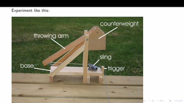
Experiment like this:

Build like this?

Inference

Most of our inference is about treatment means:

Any evidence means are not all the same?

Which ones differ?

Any pattern in differences?

How can differences be described succinctly?

Estimates/confidence intervals of means and differences.

Variability and other aspects may be of interest in specific cases.

Models

We seek the simplest model consistent with the data.

“All treatments have the same mean” is simpler than“Each treatment has its own mean.” If we cannot say that the complicated model isneeded, we take the simple model.

Sometimes we seek a more explanatory model.

“Treatment means vary linearly with temperature” is simpler than “Each treatmenthas its own mean” or even “Treatment means vary quadratically with temperature.”An explanatory model (especially a simple one) helps us understand the data.

All models are wrong; some models are useful. — George Box

We might not believe that the simple model can be completely true in some infinitelyprecise sense, but if the data are consistent with it, we use it.

Comparing models

We gauge model fit by looking at the sum of squared residuals.

We usually choose model parameters so as to minimize the sum of squared residuals.

The total sum of squares in the data SST is the sum of the model or explained sum ofsquares SSM plus the error or residual sum of squares SSE . For a fixed set of data, ifyou change the model making one SS bigger, then the other must get smaller.

SST = SSM + SSE

“All treatment means are the same” is a special case of “Each treatment has its ownmean.” “Treatment means vary linearly with temperature” is a special case of“Treatment means vary quadratically with temperature” and, indeed, of “Eachtreatment has its own mean” as well.

We say that the special case model is included in the more complicated model, orperhaps that it is a restriction of (a restricted version of) the more complicated model.

We sometimes say that the special case model is nested in the more complicatedmodel, but we will also use the descriptor “nested” in a different way later, so beware.

When we have model A included in model B, then:

1 Model B (fit by LS) always fits at least as well as model A (fit by LS), and usuallyfits better.

2 The error sum of squares from model B cannot be larger than the error sum ofsquares from model A, and is usually smaller.

3 Equivalently, the model SS for model B is always at least as large and usuallylarger than the model SS for model A.

4 The reduction in error SS going from A to B is the same as the increase in modelSS going from A to B.

ANOVA

The partitioning of the sums of squares is called Analysis of Variance, or ANOVA.

The special case model never fits as well as the larger model, but how do we decidethat it is good enough, that is, is consistent with the data?

The two basic approaches are:

Significance testing

Information Criteria

Significance testing

We will make an ANOVA table that has a row for the restricted model, a row for theincrement from the restricted model to the larger model, and a row for all of theresidual bits.

Each row in the table has a label, a sum of squares, a “degrees of freedom,” and a“Mean square.”

Degrees of freedom count free parameters. If there are r1 parameters in the meanstructure of the included model, and r2 parameters in the mean structure of the largermodel, then there are r2 − r1 parameters in the improvement from the small model tothe large model, and N − r2 parameters for residuals (error).

An MS is SS divided by DF.

The generic table looks like this (SS1 is model SS for restricted model, and SS2 ismodel SS for the large model):

Source SS DF MS

Model 1 SS1 r1 SS1/r1

Improvement fromModel 1 to Model 2 SS2 − SS1 r2 − r1 (SS2 − SS1)/(r2 − r1)

Error SSE N − r2 SSE/(N − r2)

Notation

There are simple formulae for elements of the ANOVA table for many designedexperiments.

Let yij be the jth response in treatment i . i = 1, 2, . . . , g and j = 1, 2, . . . , ni .

Let

y i• =

∑nij=1 yij

ni

be the mean response in the ith treatment, and let

y•• =

∑gi=1

∑nij=1 yij

N

be the grand mean response.

Suppose that the restricted model is the model that all treatments have the samemean, and the larger model is the model that each treatment has its own mean. Then:r1 = 1

r2 = g

SS1 = Ny••2

SS2 =∑g

i=1 niy i•2

SS2 − SS1 =∑g

i=1 ni (y i• − y••)2

SSE =∑g

i=1

∑nij=1(yij − y i•)2

and the ANOVA table is . . .

Basic ANOVA

The first four columns of the ANOVA table are:

Source SS DF MS

Overall mean Ny••2 1

Between Treatments∑g

i=1 ni (y i• − y••)2 g − 1 SSTrt/(g − 1)

Error∑g

i=1

∑nij=1(yij − y i•)2 N − g SSE/(N − g)

and the MS may be denoted MSE and MSTrt .

In fact, the line for the overall mean is so boring that it is usually left off.

Digression on Pythagorean Theorem

Note thatyij = y•• + (y i• − y••) + (yij − y i•)

Square both sides and add over all i and j and we get

g∑i=1

ni∑j=1

y2ij = Ny••2 +

g∑i=1

ni (y i• − y••)2 +

g∑i=1

ni∑j=1

(yij − y i•)2

plus a lot of sums of cross products. All those sums of cross products add to zero (thethree components of yij are perpendicular out in N-dimensional geometry so sums ofsquares add up).

Probability model

The ANOVA is just algebra, albeit algebra with statistical intent. We need aprobability model.

Assume that yij ∼ N(µi , σ2). Then,

E (MSE ) = σ2

and if the restricted model is true we also have

E (MSTrt) = σ2

If the restricted model is not good enough its expectation is larger than σ2. Thismeans that

F = MSTrt/MSE

is a test statistic for comparing the restricted model to the full model; we reject thenull if F is too big.

When the null is true and the normal distribution assumptions are correct, the F-testfollows an F-distribution with g − 1 and N − g df (note df from numerator anddenominator MS). Reject the null that the single mean model is true when the p-valuefor the F-test is too small.

We did the algebra for the single mean model and individual mean model, but the Ftest is appropriate for general restricted models versus a containing model. It’s justthat the computations are not always so clean.

Resin example in R.

Information criteria

Akaike introduced the first information criterion, AIC.

Later Bayesians added a second one, BIC.

Now there are several more.

Information criteria include a measure of how well the data fit the model (smallerbeing better) plus a penalty for using additional parameters.

Models with smaller values of AIC or BIC are better models.

Let L be the maximized likelihood for the data. This is the “probability” of the dataunder the model, with the parameters chosen to make the probability as high aspossible. This likelihood model has k parameters that we can choose. Typically theseparameters are things like treatment means, or regression coefficients, or residualvariances.

We’ll say a lot more later, but for now suffice it to say that big L is good.

AIC = −2 ln(L) + 2k

BIC = −2 ln(L) + ln(N)k

Choose a model with smaller AIC (or BIC).

In general, AIC tends to choose models with more parameters than we get fromsignificance testing, i.e., some things in the selected model might be “insignificant.”The reverse tends to be true for BIC, especially for big data sets.

Except for very small data sets, BIC penalizes additional parameters more than AIC.BIC thus tends to choose smaller models than AIC.

AIC tends to work better when all candidate models are approximate; BIC tends towork better in large samples when one of the candidate models is really the rightmodel.

Resin example in R, continued.

Parameters

You have an apartment in SE Minneapolis. You can locate it by

Latitude and longitude;

Street address (note, streets in SE are not oriented NS/EW, so this is differentthan lat/long);

Walking directions from here;

Distance and direction from here.

Four completely separate ways to identify the same place. In fact, walking directionsare not even unique!

Mean parameters suffer the same issue: there are many ways to describe/parameterizethe same set of means. Sometimes one is better than another in a particular context.Sometimes one is more understandable than another.

It is an embarrassment of riches, but as long as the parameters describe the samemeans, we are OK.

They can all be different yet still correct, but you need to know which ones you’reworking with.

Consider the resin example.

Trt (oC ) 175 194 213 231 250 All data

Average 1.933 1.629 1.378 1.194 1.057 1.465Count 8 8 8 7 6 37

If we have a single mean model, the only parameter is the overall mean µ. Ourestimate would be µ̂ = y•• = 1.465.

In the separate means model, parameters are the group means, and the estimateswould be µ̂1 = y1• = 1.933 and so on.

Sometimes we want to writeµi = µ+ αi

Where µ is some kind of “central value” and αi is a treatment effect.

We always have αi = µi − µ and α̂i = µ̂i − µ̂, but how do we define µ?

Like the walking instructions, there are many, many ways, but there are threesemi-standard ways.

Define µ Equivalent constraint

µ = µ1 α1 = 0

µ =∑

i µi

g

∑i αi = 0

µ =∑

i niµi

N

∑i niαi = 0

The first is the default in R, I find the second more interpretable, and the third isuseful in hand calculations.

The important things (µi − µj = αi − αj) are the same in all versions.

Care about µ in the single mean model; care about µi and αi − αj in the separatemeans model.

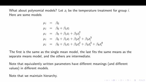
What about polynomial models? Let zi be the temperature treatment for group i .Here are some models

µi = β0

µi = β0 + β1zi

µi = β0 + β1zi + β2z2i

µi = β0 + β1zi + β2z2i + β3z

3i

µi = β0 + β1zi + β2z2i + β3z

3i + β4z

4i

The first is the same as the single mean model, the last fits the same means as theseparate means model, and the others are intermediate.

Note that equivalently written parameters have different meanings (and differentvalues) in different models.

Note that we maintain hierarchy.

But we don’t even leave polynomials in peace. Consider

µi = β0 + β1[zi − 210.0811]

+ β2[z2i − 422.9zi + 44043.5]

+ β3[z3i − 636.4z2i + 133812.3zi − 9294576.3]

This is equivalent to the cubic model on the last slide, but here the βi retain valuesand meanings as we change linear to quadratic to cubic (and you can go higher).These are orthogonal polynomials.

The moral of the story is that

Parameters are tricksy and can often be defined in many ways within a singlemean structure.

We usually only use parameters as a means to an end.

Most parameters are arbitrary, so inference on parameters (as opposed to modelcomparison or comparison of means) is also somewhat arbitrary.

R will compute the estimates as well as standard errors for various parameterizations,polynomials, orthogonal polynomials, trigonometric series, and so on. They are donecorrectly, but they retain the arbitrariness of their definition.

Back to resin.