Education Choices in Mexico: Using aStructural Model and a RandomizedExperiment to evaluate Progresa.�

Orazio P. Attanasio,yCostas Meghir,zAna Santiagox

January 2011(First version January 2001)

Abstract

In this paper we use an economic model to analyse data from a ma-jor randomised social experiment, namely PROGRESA in Mexico, andto evaluate its impact on school participation. We show the usefulnessof using experimental data to estimate a structural economic model aswell as the importance of a structural model in interpreting experimen-tal results. The availability of the experiment also allow us to estimatethe program�s general equilibrium e¤ects, which we then incorporate intoout simulations. Our main �ndings are : (i) the program�s grant has amuch stronger impact on school enrolment than an equivalent reductionin child wages; (ii) the program has a positive e¤ect on the enrollment ofchildren, especially after primary school; this result is well replicated bythe parsimonious structural model; (iii) there are sizeable e¤ects of theprogram on child wages, which, however, reduce the e¤ectiveness of theprogram only marginally; (iv) a revenue neutral change in the programthat would increase the grant for secondary school children while elimi-nating for the primary school children would have a substantially largere¤ect on enrollment of the latter, while having minor e¤ects on the former.

�This paper has bene�tted from valuable comments from referees, the editor KjetilStoresletten, Joe Altonji, Gary Becker, Esther Du�o, Jim Heckman, Hide Ichimura, PaulSchultz, Miguel Székely, Petra Todd, Ken Wolpin and many seminar audiences. Costas Meghirthanks the ESRC for funding under the Professorial Fellowship RES-051-27-0204. Orazio At-tanasio thanks the ESRC for funding under the Professorial Fellowship RES-051-27-0135. Wealso thank the ESRC Centre for Microeconomic Analysis of Public Policy at the Institute forFiscal Studies. Responsibility for any errors is ours.

yUCL, IFS and NBER.zYale, UCL, IFS, IFAU and IZAxIADB

1

1 Introduction

In 1998 the Mexican government started a remarkable new program in rural

localities. PROGRESA was one of the �rst and probably the most visible of

a new generation of interventions whose main aim is to improve the process

of human capital accumulation in the poorest communities by providing cash

transfers conditional on speci�c types of behaviour in three key areas targeted

by the program: nutrition, health and education. Arguably the largest of the

three components of the program was the education one. Mothers in the poorest

households in a set of targeted villages are given grants to keep their children in

school. In the �rst version of the program, which has since evolved and is now

called Oportunidades, the grants started in third grade and increased until the

ninth and were conditional on school enrolment and attendance. PROGRESA

was noticeable and remarkable not only for the original design but also because,

when the program begun, the Mexican government started a rigorous evaluation

of its e¤ects.

The evaluation of PROGRESA is greatly helped by the existence of a high

quality data set whose collection was started at the outset of the program,

between 1997 and 1998. The PROGRESA administration identi�ed 506 com-

munities that quali�ed for the program and started the collection of a rich

longitudinal data set in these communities. Moreover, 186 of these communities

where randomized out of the program with the purpose of providing a control

group that would enhance the evaluation. However, rather than being excluded

from the program all together, in the control villages the program was postponed

for about two years, during which period, four waves of the panel were collected.

Within each community in the evaluation sample, all households, both bene�-

2

ciaries (i.e. the poorest) and non-bene�ciaries, were covered by the survey. In

the control villages, it is possible to identify the would-be bene�ciaries were the

program to be implemented.

A better understanding of the e¤ectiveness of policies that promote school

attendance is important: de�cits in the accumulation of human capital have

been identi�ed by several commentators as one of the main reasons for the rela-

tively modest growth performance of Latin American economies in comparison,

for instance, with some of the South East Asian countries (see, for instance,

Behrman, 1999, Behrman, Duryea and Székely, 1999, 2000). For this reason,

the program we study and similar ones have received considerable attention in

Latin America.

By all accounts and evidence, the evaluation of PROGRESA, based on

the large randomized experiment described above, was highly successful (see

Schultz, 2003). Given the evaluation design, the program impacts could be es-

timated by comparing mean outcomes between treatment and control villages.

These estimates, on their own, can answer only a limited question (albeit with-

out relying on any parametric or functional form assumption), namely how did

the speci�c program implemented in the experiment a¤ect the outcomes of in-

terest. However, policy may require answers to much more re�ned questions,

such as extrapolating to di¤erent groups or altering the parameters of the initial

program.

The aim of this paper is to analyze the impact of monetary incentives on

education choices in rural Mexico; to discuss e¤ective design of interventions

aimed at increasing school enrolment of poor children; and to illustrate the ben-

e�ts of combining randomised experiments with structural models. To achieve

3

these goals, we estimate a simple structural model of education choices using

the data from the PROGRESA randomised experiment. We then use the model

to simulate the e¤ect of changes to some of the parameters of the program.

PROGRESA e¤ectively changes the relative price of education and child

labour in a controlled and exogenous fashion. A tightly parametrized model,

under suitable restrictions (see below), could identify the e¤ect of the program

even before its implementation, using variation in the opportunity cost of school-

ing (i.e. the wage) across communities where the program is not available. This

is the strategy followed, in a recent paper, by Todd and Wolpin (2006) (TW

henceforth). They identify the impact of the program from variation in child

wages across villages in which the program is not implemented and estimate

their model without using the variability induced by the PROGRESA. Their

approach does not require experimental variation other than as a validation for

their model.

Like TW, we estimate a structural model, but our approach and objectives

are di¤erent. We use both treatment and control villages exploiting the variation

in the grant induced by the randomized experiment to estimate a more �exible

speci�cation than could be estimated without the program: critically, we do

not restrict the e¤ect of the grant to be the same as that of wages. Indeed we

�nd that o¤ering the conditional grant has four times the e¤ect of an equivalent

reduction in the earnings opportunities (wage) of children.

There are many reasons why the grant might have a di¤erent e¤ect from

the wage; these relate to the structure of preferences, the nature of within

household decision making and the perception of the grant. In some cases,

such nonseparability can only be taken into account using the variation in a

4

school grant such as that induced by the experiment. This is speci�cally the

case when income pooling fails within the household and the marginal value of

income depends on the activity of the child (nonseparability between income

and education).1

Thus the use of non-experimental data to carry out ex ante evaluation, with

no variation in school grants, requires additional assumptions: one needs to

assume that child and household income have the same e¤ect on utility, condi-

tional on the activity of the child. This assumption allows one to aggregate other

household and child income into one single pooled income measure as TW do.

A violation of such an assumption may relate to preferences or to within house-

hold allocations. For example, while the PROGRESA grant is always handed

over to the mother, income from child labour may be under the control of the

father or even of the child if she/he is older. In all these cases a peso of child

income from work is di¤erent from a peso of child income from a school grants

programme and both are potentially di¤erent from a peso of income from other

sources. At least in the context of this population, our results clearly indicate

that such nonseparabilities are crucially important.

Does this mean that ex-ante evaluation is infeasible in this context? This

would be a rash conclusion, because there may well be suitable observational

data that could help resolve the issues we raise; for example data from a popula-

tion where some children receive scholarships of varying amounts: given suitable

exogeneity assumptions, in this case there would be income attached to attend-

ing schooling and the necessary variation to identify its e¤ects; this is not the

case in the PROGRESA sample of controls. But even if such variation exists in

1For tests of income pooling see amongs others Thomas (1990) or Blundell, Magnac, Chi-appori and Meghir (2007).

5

the data, experimental information can clearly be important for understanding

behaviour, if anything because the variation induced by the experiment is guar-

anteed to be exogenous. Thus, one can think of using experimental variation

and indeed designing experiments to generate such variability so as to estimate

more credibly structural models capable of richer policy analysis. In this sense,

our work draws from the tradition of Orcutt and Orcutt (1968), who advocate

precisely this approach, which found an early expression in the work based on

the negative income tax experiments, such as in Burtless and Hausman (1978)

and Mo¢ tt (1979). The general point we make is that the experimental variation

can help identify economic e¤ects under more general conditions than the ob-

servational data, while the structural model can help provide an interpretation

of the experimental results and broaden the usefulness of the experiment.

The fact that we estimate a model that, in some dimensions, is more general

than the one by TW and that requires the explicit use of the experimental

variation to be identi�ed is not the only di¤erence between the two papers. Our

approach considers explicitly and estimates the general equilibrium e¤ects that

the program might have on the wages of young children. As mentioned above,

PROGRESA was randomized across localities, rather than across households.

As these localities are isolated from each other, this experimental design also

a¤ords the possibility of estimating general equilibrium e¤ect induced by the

program. Although some papers in the literature (see, for instance, Angelucci

and De Giorgi, 2009) have looked at the impact of PROGRESA on prices and

other village level variables, perhaps surprisingly, no study has considered, as

far as we know, the e¤ect that the program has had on children wages. One

could imagine that, if the program is e¤ective in increasing school participation,

6

a reduction in the supply of child labour could result in an increase in child

wages which, in turn, would result in an attenuation of the program�s impact.

Here we estimate this impact (taking into account the fact that child wages

are observed only for the selected subset of children who actually work) and

establish that the program led to an increase in these wages in the treatment

municipalities, by decreasing the labour supply of children. We incorporate

these general equilibrium impacts within our model and in our simulations.

Finally, there are also di¤erences in the estimation approach, as well as in

the speci�cation of the models, between this paper and that of TW. Both our

model and TW�s include the presence of habits in the utility from schooling.

This creates an initial condition problem in the estimation of the structural

model. While TW tackle this issue by functional form assumptions and the im-

plied nonlinearities, we also exploit the increasing availability of schooling as an

instrument to control for the initial conditions problem so as to better disentan-

gle state dependence from unobserved heterogeneity. As for the speci�cation,

TW�s model solves a family decision problem, including trade-o¤s between chil-

dren and fertility, which we do not. Considering fertility e¤ects is potentially

interesting. However, it should be pointed out that the programme did not

have any e¤ects on fertility.2 What has informed our modelling choices is the

focus on using the incentives introduced by the programme in some localities to

identify in a credible fashion our education choice model.

The rest of the paper is organized as follows. In Section 2, we present

the main features of the program and of the evaluation survey we use. In

section 3, we present some simple results on the e¤ectiveness of the program

2TW�s model of fertility is identi�ed only using the observed cross sectional variation whichmay not necessarily re�ect exogenous di¤erences in incentives.

7

based on the comparison of treatment and control villages. In section 4, we

present a structural dynamic model of education choices and describe its various

components. Section 5 brie�y discusses the estimation of the model. Section

6 presents the results we obtain from the estimation of our model. We also

report the results of a version of the model that imposes some restrictions that

approximate the model estimated by TW. Section 7 uses the model to perform a

number of policy simulations that could help to �ne-tune the program. Finally,

Section 8 concludes the paper with some thoughts about open issues and future

research.

2 The PROGRESA program.

PROGRESA was started in 1997 by the Zedillo administration. The program

introduced a number of incentives and conditions with which participant house-

holds had to comply to keep receiving the program�s bene�ts. At the same

time the administration put in place a quantitative evaluation of the program�s

impact based on a randomized design,

2.1 The speci�cs of the PROGRESA program

PROGRESA is the Spanish acronym for �Health, Nutrition and Education�,

that are the three main areas of the program. PROGRESA is one of the �rst

and probably the best known of the so-called �conditional cash transfers�, which

aim at alleviating poverty in the short run while at the same time fostering the

accumulation of human capital to reduce it in the long run. This is achieved

by transferring cash to poor households under the condition that they engage

in behaviours that are consistent with the accumulation of human capital: the

nutritional subsidy is paid to mothers that register the children for growth and

8

development check ups and vaccinate them as well as attend courses on hygiene,

nutrition and contraception. The education grants are paid to mothers if their

school age children attend school regularly.

The program has received considerable attention and publicity. More re-

cently programs similar to and inspired by PROGRESA have been implemented

in Colombia, Honduras, Nicaragua, Argentina, Brazil, Turkey and other coun-

tries. Rawlings (2004) contains a survey of some of these programs. Skou�as

(2001) provides additional details on PROGRESA and its evaluation.

PROGRESA is �rst targeted at the locality level. Within each community,

then the program is targeted by proxy means testing. Individual households

in a targeted community could qualify or not for the program, depending on

a single indicator, the �rst principal component of a number of variables (such

as income, house type, presence of running water, and so on). Eligibility was

determined in two steps. First, a general census of the PROGRESA localities

measured the variables needed to compute the indicator and each household

was de�ned as �poor� or �not-poor� (where �poor� is equivalent to eligibility).

Subsequently, in March 1998, an additional survey was carried out and some

households were added to the list of bene�ciaries. This second set of bene�ciary

households are called �densi�cados�. Fortunately, the re-classi�cation survey was

operated both in treatment and control towns.

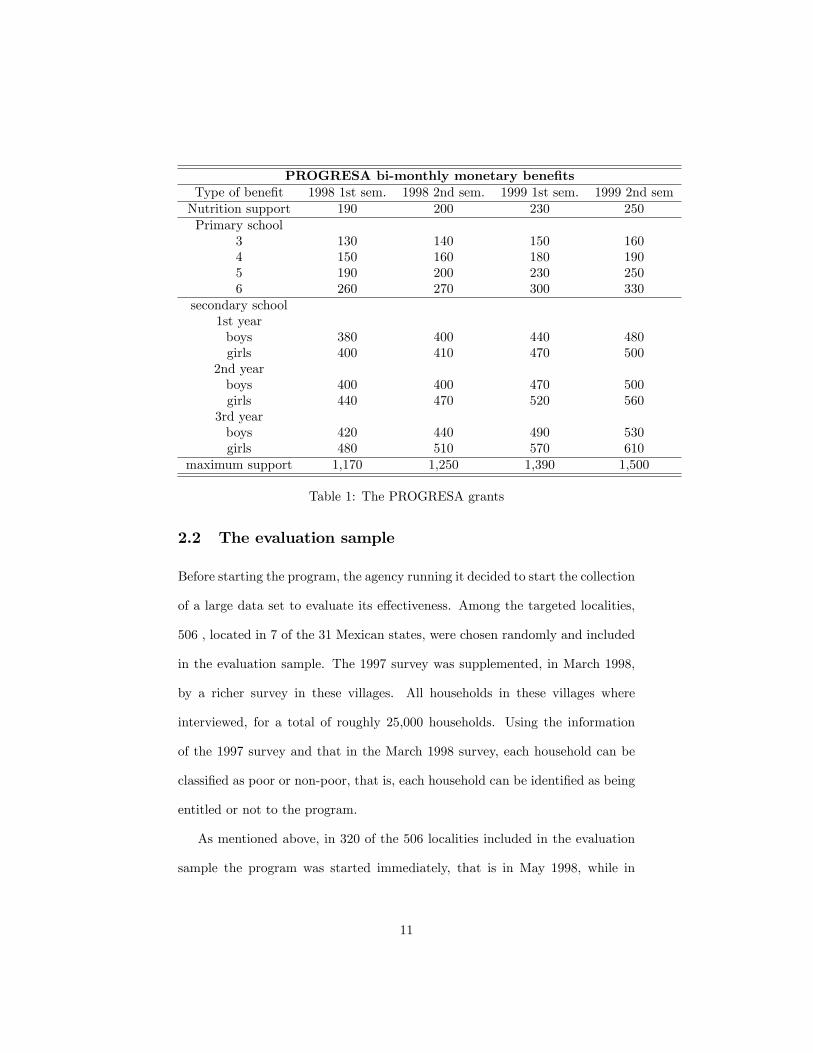
The largest component of the program is the education one. Bene�ciary

households with school age children receive grants conditional on school at-

tendance. The size of the grant increases with the grade and, for secondary

education, is slightly higher for girls than for boys. In Table 1, we report the

grant structure. All the �gures are in current pesos, and can be converted in US

9

dollars at approximately an exchange rate of 10 pesos per dollar. In addition

to the (bi) monthly payments, bene�ciaries with children in school age receive

a small annual grant for school supplies.

For logistic and budgetary reasons, the program was phased in slowly but

is currently very large. In 1998 it was started in less than 10,000 localities.

However, at the end of 1999 it was implemented in more than 50,000 localities

and had a budget of about US$777 million or 0.2% of Mexican GDP. At that

time, about 2.6 million households, or 40% of all rural families and one ninth

of all households in Mexico, were included in the program. Subsequently the

program was further expanded and, in 2002-2003 was extended to some urban

areas.

The program represents a substantial help for the bene�ciaries. The nu-

tritional component of 100 pesos per month (or 10 US dollars) in the second

semester of 1998, corresponded to 8% of the bene�ciaries�income in the evalu-

ation sample.

As mentioned above, the education grants are conditional to school enrol-

ment and attendance of children, and can be cumulated within a household up

to a maximum of 625 pesos (or 62.5 dollars) per month per household or 52% of

the average bene�ciary�s income. The average grant per household in the sam-

ple we use was 348 pesos per month for households with children and 250 for

all bene�ciaries or 21% of the bene�ciaries income. To keep the grant, children

have to attend at least 85% of classes. Upon not passing a grade, a child is still

entitled to the grant for the same grade. However, if the child fails the grade

again, it looses eligibility.

10

PROGRESA bi-monthly monetary bene�tsType of bene�t 1998 1st sem. 1998 2nd sem. 1999 1st sem. 1999 2nd semNutrition support 190 200 230 250Primary school

3 130 140 150 1604 150 160 180 1905 190 200 230 2506 260 270 300 330

secondary school1st yearboys 380 400 440 480girls 400 410 470 500

2nd yearboys 400 400 470 500girls 440 470 520 560

3rd yearboys 420 440 490 530girls 480 510 570 610

maximum support 1,170 1,250 1,390 1,500

Table 1: The PROGRESA grants

2.2 The evaluation sample

Before starting the program, the agency running it decided to start the collection

of a large data set to evaluate its e¤ectiveness. Among the targeted localities,

506 , located in 7 of the 31 Mexican states, were chosen randomly and included

in the evaluation sample. The 1997 survey was supplemented, in March 1998,

by a richer survey in these villages. All households in these villages where

interviewed, for a total of roughly 25,000 households. Using the information

of the 1997 survey and that in the March 1998 survey, each household can be

classi�ed as poor or non-poor, that is, each household can be identi�ed as being

entitled or not to the program.

As mentioned above, in 320 of the 506 localities included in the evaluation

sample the program was started immediately, that is in May 1998, while in

11

the remaining 186 it was started almost two years later. The 320 �treatment

localities�were chosen randomly.

An extensive survey was carried out in the evaluation sample: after the initial

data collection between the end of 1997 and the beginning of 1998, an additional

4 instruments were collected in November 1998, March 1999, November 1999

and April 2000. Within each village in the evaluation sample, the survey covers

all the households and collects extensive information on consumption, income,

transfers and a variety of other variables. For each household member, including

each child, there is information about age, gender, education, current labour

supply, earnings, school enrolment, and health status. The household survey is

supplemented by a locality questionnaire that provides information on prices of

various commodities, average agricultural wages (both for males and females)

as well as institutions present in the village and distance of the village from the

closest primary and secondary school (in kilometers and minutes).

At the time of the 1997 survey, each household in the treatment and control

villages was de�ned either as eligible or non eligible. Subsequently, in March

1998 before the start of the program, some of the non-eligible household were

re-classi�ed as eligible. However, a considerable fraction of the newly eligible

households, due to administrative delays, did not start receiving the program

until much later. In some of the results we present below, we distinguish these

households. In the estimation of the structural model we consider as bene�ciary

a household that actually receives the program.

12

3 Measuring the impact of the program: treat-ment versus control villages.

As PROGRESA was assigned randomly between treatment and control villages

during the expansion phase of the program, it is straightforward to use the

evaluation sample to estimate the impact of the conditional cash transfers on

school enrolment. Randomization implies that control and treatment sample

are statistically identical and estimates of program impacts can be obtained by

a simple comparison of means. However, such an exercise estimates the impact

of the program as a whole, without specifying the mechanisms through which

it operates.

The availability of baseline, pre-program data, allows one to check whether

the evaluation sample is balanced between treatment and control groups both

in terms of pre-program outcomes and in terms of other observable background

characteristics. This exercise was performed by Behrman and Todd (1999), who

explored a wide range of variables at baseline. The data includes information on

programme eligibility for both treatment and control villages at baseline. This

allows us to make the comparisons separately for eligible and non-eligible house-

holds. Behrman and Todd (1999) indicate that, by and large, the treatment and

control samples are very well balanced. However, there seem to be some pre-

program di¤erences in school enrolment among non eligible households. While

it is not clear why such a di¤erence arises, it might be important to control for

these initial di¤erences when estimating impacts.

In this section, we present some estimates of the impact of PROGRESA on

school enrolment. These impacts have been widely studied: the IFPRI (2000)

report estimates of program impacts on a wide set of outcomes, while Schultz

13

(2003) presents a complete set of results on the impact of the program on school

enrolment, which are substantially similar to those presented here. Here our

focus is on some aspects of the data that are pertinent to our model and to the

sample we use to estimate it. And more importantly, by describing the impacts

of the program in the sample we use to estimate our structural model, we set

the mark against which it will be �tted.

As our structural model will be estimated on boys, we report only the results

for them. The e¤ects for girls are slightly higher but not substantially di¤erent

from those reported here for boys. As we will be interested in how the e¤ect

of the grant varies with age, we also report the results for di¤erent age groups,

although when we consider individual ages, some of the estimates are quite

imprecise.

In Table 2 we report the estimated impact for the boys of each age obtained

comparing treatment and control villages in October 1998. In the last two rows,

we also report the average impacts on boys aged 12 to 15 (which is an age group

on which Todd and Wolpin, 2006 focus) and on boys aged 10 to 16, that is our

entire sample. In the �rst column of the Table, we report enrolment rates among

eligible (as of 1997) boys in control villages. In the second column, we show the

estimated impacts obtained for boys from households that were declared eligible

in 1997 (poor 97). In the third column, we report the results for the boys in all

eligible households, including those reclassi�ed in March 1998. Finally, in the

third column, we report the impacts on the non-eligible children.

The experimental impacts show that the e¤ect of the PROGRESA program

on enrolment has a marked inverted U shape. The program impact is small and

not signi�cantly di¤erent from zero at age 10. It increases considerably past

14

age 10, to peak at age 14, where our point estimates indicates an impact of 14

percentage points on boys whose households were classi�ed as eligible in 1997.

The impact then declines for higher ages, probably a consequence of the fact

that the grant was not available, in the �rst version of the program, past grade

9. The average impact for the boys in our sample (aged 10 to 16) is about 5

percentage point, while for the boys aged 12 to 15 is, on average, as high as

6.6%.

The impact on the households classi�ed as poor in 1997 is slightly higher than

on all eligible households, probably a re�ection that the impact might be higher

for poorer families and the fact that, some of the families that were reclassi�ed

as eligible in March 1998 (after being classi�ed as non eligible in 1997), did not

receive the program immediately, due to administrative di¢ culties.

A surprising feature of Table 2 is the measured impact on non eligible chil-

dren. Although noisy, the estimates for some age groups indicate a large impact

on non-eligible boys. Indeed, for the age group 10-16, the e¤ect is even larger

than for the eligible children, at almost 8%. While one could think of the pos-

sibility of spill-over e¤ects that would generate positive e¤ects on non-eligible

children, the size of the impacts we measure in Table 2 is such that this type of

explanation is implausible. As we mentioned above, however, if one compares

school enrolment rates in 1997 between treatment and control villages, one �nds

that, among non-eligible households, they are signi�cantly higher (statistically

and substantially) in treatment villages than in control villages. This is partic-

ularly so for children aged 12 to 16. Instead, enrolment rates in 1997 among

eligible children, are statistically identical in treatment and control villages. It

is therefore possible that the observed di¤erence in enrolment rates among non-

15

eligible households is driven by pre-existing di¤erences between treatment and

control towns.

The reason for the di¤erence in enrolment rates among boys (and girls)

in non eligible households between treatment and control villages is not clear.

Within our structural model, we account for it by considering one speci�cation

which incorporates an unobserved cost component for non-eligible households

in control villages. As for measuring the e¤ect of the program as in Table 2,

one can use the 1997 data to obtain a di¤erence in di¤erence estimates of its

impacts. We report the results of such an exercise in Table 6 in the Appen-

dix. In this table, the pattern of the impacts among eligible children is largely

una¤ected (as to be expected given the lack of signi�cant di¤erences between

treatment and control villages at baseline for these children). The impacts on

the non-eligible children, however, become insigni�cant. This evidence justi�es

the interpretation of the evidence in the last column of Table 2 as being caused

by pre-existing unobservable di¤erences for non eligible children and justi�es

our use of a �non eligible control�dummy in our empirical speci�cation.

4 The model

We use a simple dynamic school participation model. Each child, (or his/her

parents) decide whether to attend school or to work taking into account the

economic incentives involved with such choices. Parents are assumed here to

act in the best interest of the child and consequently we do not admit any

interactions between children. We assume that children have the possibility

16

Di¤erence estimates of the impact of PROGRESAon boys school enrolment

Age Groupenrolment rates incontrol villages (eligible)

Impact onPoor 97

Impact onPoor 97-98

Impact onnon-elig.

10 0.9510.0047(0.013)

0.0026(0.011)

0.0213(0.021)

11 0.9260.0287(0.016)

0.0217(0.015)

-0.0195(0.019)

12 0.8260.0613(0.024)

0.0572(0.022)

0.0353(0.043)

13 0.7800.0476(0.030)

0.0447(0.027)

0.0588(0.060)

14 0.5840.1416(0.039)

0.1330(0.035)

0.0672(0.061)

15 0.4550.0620(0.042)

0.0484(0.039)

0.1347(0.063)

16 0.2920.0304(0.038)

0.0355(0.036)

0.1063(0.067)

12-15 0.6290.0655(0.027)

0.0720(0.024)

0.0668(0.022)

10-16 0.7080.0502(0.018)

0.0456(0.015)

0.0810(0.026)

Standard errors in parentheses are clustered at the locality level.

Table 2: Experimental Results October 1998

17

of going to school up to age 17. All formal schooling ends by that time. In

the data, almost no individuals above age 17 are in school. We assume that

children who go to school do not work and vice-versa. We also assume that

children necessarily choose one of these two options. If they decide to work they

receive a village/education/age speci�c wage. If they go to school, they incur

a (utility) cost (which might depend on various observable and unobservable

characteristics) and, with a certain probability, progress a grade. At 18, every-

body ends formal schooling and reaps the value of schooling investments in the

form of a terminal value function that depends on the highest grade passed.

The PROGRESA grant is easily introduced as an additional monetary reward

to schooling, that would be compared to that of working.

The model we consider is dynamic for two main reasons. First, the fact

that one cannot attend regular school past age 17 means that going to school

now provides the option of completing some grades in the future: that is a six

year old child who wants to complete secondary education has to go to school

(and pass the grade) every single year, starting from the current. This source of

dynamics becomes particularly important when we consider the impact of the

PROGRESA grants, since children, as we saw above, are only eligible for six

grades: the last three years of primary school and the �rst three of secondary.

Going through primary school (by age 14), therefore, also �buys�eligibility for

the secondary school grants. Second, we allow for state dependence: the number

of years of schooling a¤ects the utility of attending in this period. We explicitly

address the initial conditions problem that arises from such a consideration

and discuss the related identi�cation issues at length below. State dependence

is important because it may be a mechanism that reinforces the e¤ect of the

18

grant.

Before discussing the details of the model it is worth mentioning that using

a structural approach allows us to address the issue of anticipation e¤ects and

the assumptions required for their identi�cation. PROGRESA as well as other

randomized experiments or pilot studies create a control group by delaying

the implementation of the program in some areas, rather than excluding them

completely. It is therefore possible that the control villages react to the program

prior to its implementation, depending on the degree to which they believe they

will eventually receive it. A straight comparison between treatment and control

areas may then underestimate the impact of the program. A structural model

that exploits other sources of variation, such as the variation of the grant with

age may be able to estimate the extent of anticipation e¤ects. We investigated

this with our model by examining its �t under di¤erent assumptions about

when the controls are expecting to receive payment. As it turns out we �nd no

evidence of anticipation e¤ects in our data. This is not surprising because there

was no explicit policy announcing the future availability of the grants. The

absence of evidence on anticipation e¤ects, however, is consistent both with no

information about the future availability of the program and with an inability to

take advantage of future availability due, for instance, to liquidity constraints.

4.1 Instantaneous utilities from schooling and work

The version of the model we use assumes linear utility. In each period, going

to school involves instantaneous pecuniary and non-pecuniary costs, in addition

to losing the opportunity of working for a wage. The current bene�ts come

from the utility of attending school and possibly, as far as the parents are

concerned, by the child-care services that the school provides during the working

19

day. As mentioned above, the bene�ts are also assumed to be a function of past

attendance. The direct costs of attending school are the costs of buying books

etc. as well as clothing items such as shoes. There are also transport costs to

the extent that the village does not have a secondary school. For households

who are entitled to PROGRESA and live in a treatment village, going to school

involves receiving the grade and gender speci�c grant.

As we are using a single cross section, we use the notation t to signify the

age of the child in the year of the survey. Variables with a subscript t may

be varying with age. Denote the utility of attending school for individual i in

period t, who has already attended edit years, as usit: We posit:

usit = Y sit + �git (1)

Y sit = �si + as0zit + b

sedit + 1(pit = 1)�pxpit + 1(sit = 1)�

sxsit + "sit

where git is the amount of the grant an individual is entitled to; it will be equal

to zero for non-eligible individuals and for control localities. Y sit represents the

remaining pecuniary and non pecuniary costs or gains from attending school.

zit is a vector of taste shifter variables, including parental background, age and

state dummies. Household income may also a¤ect education choices, particu-

larly when parents are the decision makers because they need to make transfers

to their child, which they may not be able to recover later in life. However,

household income is likely to be endogenous and since we are not estimating a

complete model of household behaviour these household characteristics can be

interpreted both as re�ecting earnings ability of the household members as well

as tastes.

20

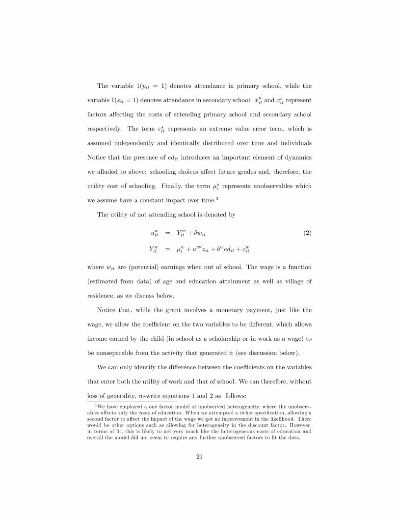
The variable 1(pit = 1) denotes attendance in primary school, while the

variable 1(sit = 1) denotes attendance in secondary school. xpit and x

sit represent

factors a¤ecting the costs of attending primary school and secondary school

respectively. The term "sit represents an extreme value error term, which is

assumed independently and identically distributed over time and individuals

Notice that the presence of edit introduces an important element of dynamics

we alluded to above: schooling choices a¤ect future grades and, therefore, the

utility cost of schooling. Finally, the term �si represents unobservables which

we assume have a constant impact over time.3

The utility of not attending school is denoted by

uwit = Y wit + �wit (2)

Y wit = �wi + aw0zit + b

wedit + "wit

where wit are (potential) earnings when out of school. The wage is a function

(estimated from data) of age and education attainment as well as village of

residence, as we discuss below.

Notice that, while the grant involves a monetary payment, just like the

wage, we allow the coe¢ cient on the two variables to be di¤erent, which allows

income earned by the child (in school as a scholarship or in work as a wage) to

be nonseparable from the activity that generated it (see discussion below).

We can only identify the di¤erence between the coe¢ cients on the variables

that enter both the utility of work and that of school. We can therefore, without

loss of generality, re-write equations 1 and 2 as follows:3We have employed a one factor model of unobserved heterogeneity, where the unobserv-

ables a¤ects only the costs of education. When we attempted a richer speci�cation, allowing asecond factor to a¤ect the impact of the wage we got no improvement in the likelihood. Therewould be other options such as allowing for heterogeneity in the discount factor. However,in terms of �t, this is likely to act very much like the heterogeneous costs of education andoverall the model did not seem to require any further unobserved factors to �t the data.

21

usit = �git + �i + a0zit + bedit + 1(pit = 1)�

pxpit + 1(sit = 1)�sxsit + "it(3)

uwit = �wit (4)

where a = as�aw; b = bs�bw; = �=�; �i = �si ��wi ; "it = "sit�"wit: The error

term "it, the di¤erence between two extreme value distributed random variables

and as such is distributed as a logistic. We will assume that �i is a discrete

random variable whose points of support and probabilities will be estimated

empirically. Finally note that all time-varying exogenous variables are assumed

to be perfectly foreseen when individuals consider trade-o¤s between the present

and the future.

The coe¢ cient measures the impact of the grant as a proportion of the

impact of the wage on the education decision. The grant (which is a function

of the school grade currently attended - as in Table 1) is suitably scaled so as

to be comparable to the wage. If = 1; the e¤ect of the grant on utility and

therefore on schooling choices, would be the same as that of the wage. If this

was the case, the e¤ect of the program could be estimated using data only from

the control communities in which it does not operate, based on the estimate of

�. This is the strategy used by TW. However, one can think of many simple

models in which there is every reason to expect that the impact of the grant

will be di¤erent to that of the wage.

The issue can be illustrated easily within a simple static model. As in our

framework, we assume that utility depends on whether the child goes to school

or not. Moreover we assume that this decision a¤ects the budget constraint. In

particular we have:

22

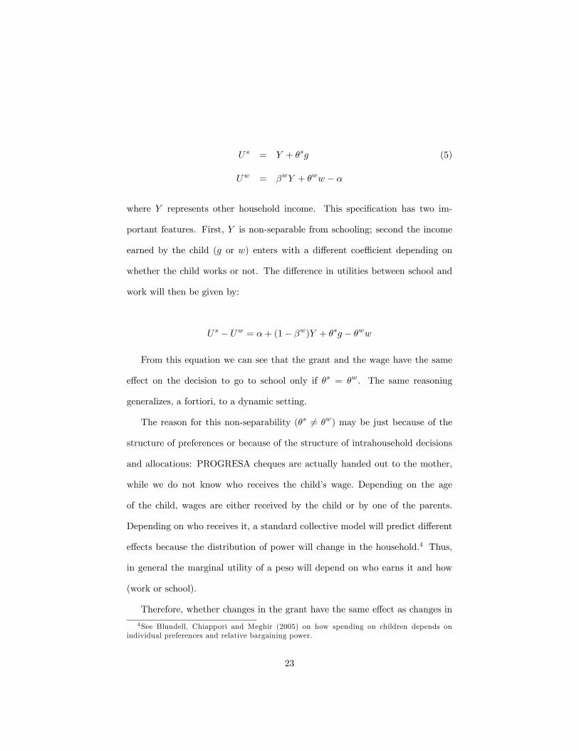
Us = Y + �sg (5)

Uw = �wY + �ww � �

where Y represents other household income. This speci�cation has two im-

portant features. First, Y is non-separable from schooling; second the income

earned by the child (g or w) enters with a di¤erent coe¢ cient depending on

whether the child works or not. The di¤erence in utilities between school and

work will then be given by:

Us � Uw = �+ (1� �w)Y + �sg � �ww

From this equation we can see that the grant and the wage have the same

e¤ect on the decision to go to school only if �s = �w. The same reasoning

generalizes, a fortiori, to a dynamic setting.

The reason for this non-separability (�s 6= �w) may be just because of the

structure of preferences or because of the structure of intrahousehold decisions

and allocations: PROGRESA cheques are actually handed out to the mother,

while we do not know who receives the child�s wage. Depending on the age

of the child, wages are either received by the child or by one of the parents.

Depending on who receives it, a standard collective model will predict di¤erent

e¤ects because the distribution of power will change in the household.4 Thus,

in general the marginal utility of a peso will depend on who earns it and how

(work or school).

Therefore, whether changes in the grant have the same e¤ect as changes in

4See Blundell, Chiappori and Meghir (2005) on how spending on children depends onindividual preferences and relative bargaining power.

23

child wages, is an empirical matter. Using the experiment we are able to test

whether the grant and the wage have the same e¤ect on school enrolment. The

design of the experiment allows us to address this important issue.

A number of alternative approaches to the evaluation of PROGRESA-type

interventions are possible in the context of this simple speci�cation. Under the

income pooling restriction that �s = 1 and �w = �w � �, the e¤ect of the

grant can be identi�ed even with g = 0, o¤ the variation of total household

income, which includes the wage for working children. Such an identi�cation

strategy does not require the experiment and uses the exogenous variation in Y

to identify the e¤ect of the intervention. Alternatively one can substitute out Y

as a function of characteristics and unobserved heterogeneity (as we do) which

leaves two parameters driving the incentives to work or go to school, i.e. �s

and �w. In this case, identi�cation either requires variation in g, say through

the experiment, or a restriction that �s = �w, in which case the experimental

variation is not needed. We use variation in g: In doing so our model imposes

non of the restrictions above and does not impose the exogeneity of household

income.

Within the context of this simple static model, TW can be described as

imposing �s = �w. They also impose the restriction that other household income

Y is exogenous and can be aggregated with child income. This leads to a model

where schooling is determined by a comparison of household income in the two

states to the costs of schooling. We estimate a version of our model on the

control group only, as TW do, based on the restriction that �s = �w to show

how such a restriction impacts policy implications.5

5The TW model is more complicated than the static equivalent implies. First they in-clude habits as we do. They allow the marginal utility of household income to depend on

24

By demonstrating the scope of combining experimental data with structural

models we hope to make it standard both to analyse experiments using struc-

tural models and to design experiments so as to enable the estimation of richer

models.

Our sample includes both eligible and ineligible individuals. Eligibility is

determined on the basis of a number of observable variables that might a¤ect

schooling costs and utility. To take into account the possibility of these system-

atic di¤erences, we also include in equation 3 (among the z variables) a dummy

for eligibility (which obviously is operative both in treatment and control local-

ities).

As we discussed in Section 3, there seems to be some di¤erences in pre-

program enrolment rates between treatment and control localities. As we do

not have an obvious explanation for these di¤erences, we use two alternative

strategies. First we control for them by adding to the equation for the schooling

utility (3) a dummy for treatment villages. Obviously such a dummy will absorb

some of the exogenous variability induced by the experiment. We discuss this

issue when we tackle the identi�cation question in the next section. A less ex-

treme approach, justi�ed by the fact that most of the unexplained di¤erences in

pre-program enrollment is observed among non-eligible household, we introduce

a dummy for this group only.

4.2 Uncertainty

There are two sources of uncertainty in our model. The �rst is an iid shock to

schooling costs, modelled by the (logistic) random term "it: Given the structure

accumulated schooling, while still imposing within period separability. Finally they add otherelements to the model, such as fertility decisions and tradeo¤s between kids in the schoolingdecision.

25

of the model, having a logistic error in the cost of going to school is equivalent

to having two extreme value errors, one in the cost of going to school and

one in the utility of work. Although the individual knows "it in the current

period,6 she does not know its value in the future. Since future costs will a¤ect

future schooling choices, indirectly they a¤ect current choices. Notice that the

term �i; while known (and constant) for the individual, is unobserved by the

econometrician.

The second source of uncertainty originates from the fact that the pupil may

not be successful in completing the grade. If a grade is not completed success-

fully, we assume that the level of education does not increase. We assume that

the probability of failing to complete a grade is exogenous and does not depend

on the willingness to continue schooling. We allow however this probability to

vary with the grade in question and with the age of the individual and we as-

sume it known to the individual.7 We estimate the probability of failure for

each grade as the ratio of individuals who are in the same grade as the year

before at a particular age. Since we know the completed grade for those not

attending school we include these in the calculation - this may be important

since failure may discourage school attendance. In the appendix we provide a

Table with our estimated probabilities of passing a grade.

6We could have introduced an additional residual term "wit in equation 2. Because whatmatters for the �t of the model is only the di¤erence between the current (and future) utilityof schooling and working, assuming that both "it and "

wit were distributed as an extreme value

distribution is equivalent to assuming a single logistic residual.7Since we estimate this probability from the data we could also allow for dependence on

other characteristics.

26

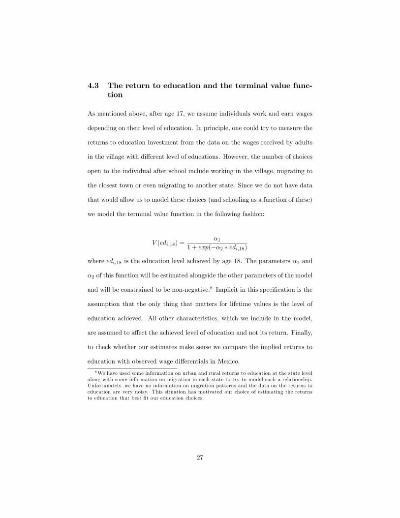
4.3 The return to education and the terminal value func-tion

As mentioned above, after age 17, we assume individuals work and earn wages

depending on their level of education. In principle, one could try to measure the

returns to education investment from the data on the wages received by adults

in the village with di¤erent level of educations. However, the number of choices

open to the individual after school include working in the village, migrating to

the closest town or even migrating to another state. Since we do not have data

that would allow us to model these choices (and schooling as a function of these)

we model the terminal value function in the following fashion:

V (edi;18) =�1

1 + exp(��2 � edi;18)

where edi;18 is the education level achieved by age 18. The parameters �1 and

�2 of this function will be estimated alongside the other parameters of the model

and will be constrained to be non-negative.8 Implicit in this speci�cation is the

assumption that the only thing that matters for lifetime values is the level of

education achieved. All other characteristics, which we include in the model,

are assumed to a¤ect the achieved level of education and not its return. Finally,

to check whether our estimates make sense we compare the implied returns to

education with observed wage di¤erentials in Mexico.

8We have used some information on urban and rural returns to education at the state levelalong with some information on migration in each state to try to model such a relationship.Unfortunately, we have no information on migration patterns and the data on the returns toeducation are very noisy. This situation has motivated our choice of estimating the returnsto education that best �t our education choices.

27

4.4 Value functions

Since the problem is not separable overtime, schooling choices involve comparing

the costs of schooling now to its future and current bene�ts. The latter are

intangible preferences for attending school including the potential child care

bene�ts that parents may enjoy.

We denote by I 2 f0; 1g the random increment to the grade which results

from attending school at present. If successful, then I = 1; otherwise I = 0:We

denote the probability of success at age t for grade ed as pst (edit).

Thus the value of attending school for someone who has completed success-

fully edi years in school and is of age t already and has characteristics zit is

V sit(editj�it) = usit + �fpst (edit + 1)Emax�V sit+1 (edit + 1) ; V

wit+1 (edit + 1)

�+(1� pst (edit + 1))Emax

�V sit+1 (edit) ; V

wit+1 (edit)

�g

where the expectation is taken over the possible outcomes of the random shock

"it and where �it is the entire set of variables known to the individual at period

t and a¤ecting preferences and expectations the costs of education and labour

market opportunities. The value of working is similarly written as

V wit (editj�it) = uwit + �Emax�V sit+1 (edit) ; V

wit+1 (edit)

The di¤erence between the �rst terms of the two equations re�ects the current

costs of attending, while the di¤erence between the second two terms re�ects the

future bene�ts and costs of schooling. The parameter � represents the discount

factor. In practice, since we do not model savings and borrowing explicitly

this will re�ect liquidity constraints or other factors that lead the households to

disregard more or less the future.

Given the terminal value function described above, these equations can be

used to compute the value of school and work for each child in the sample

28

recursively. These formulae will be used to build the likelihood function used

to estimate the parameters of this model.

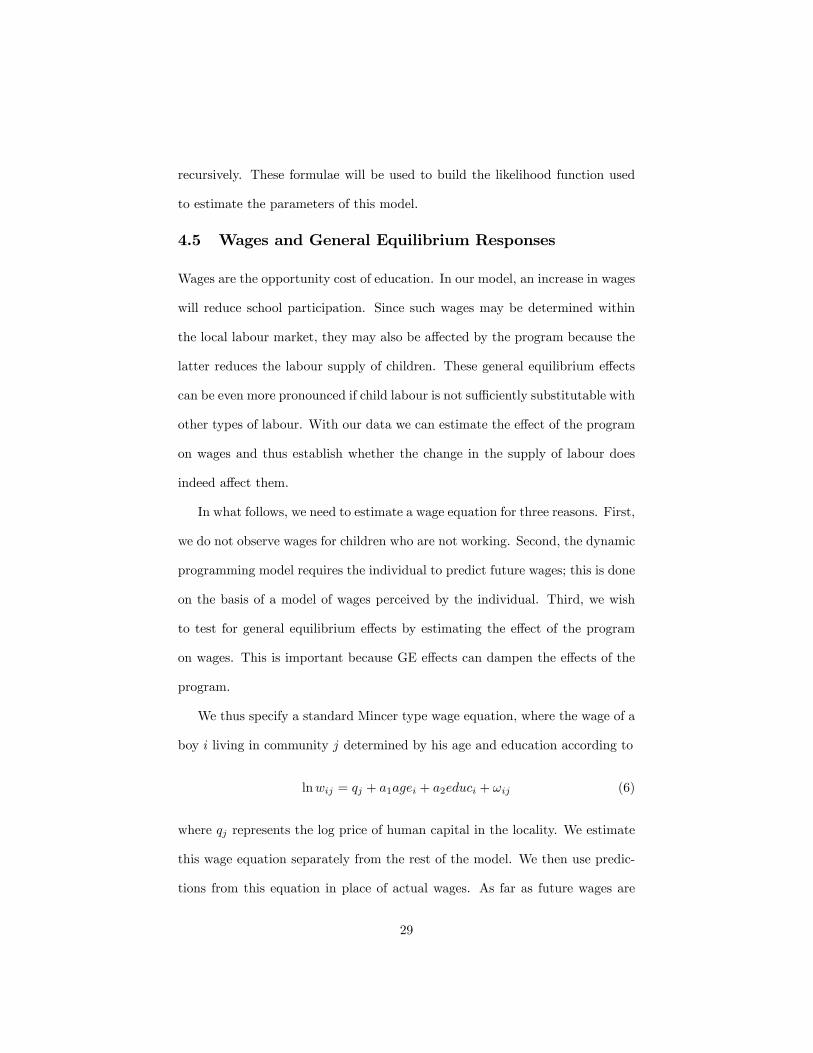
4.5 Wages and General Equilibrium Responses

Wages are the opportunity cost of education. In our model, an increase in wages

will reduce school participation. Since such wages may be determined within

the local labour market, they may also be a¤ected by the program because the

latter reduces the labour supply of children. These general equilibrium e¤ects

can be even more pronounced if child labour is not su¢ ciently substitutable with

other types of labour. With our data we can estimate the e¤ect of the program

on wages and thus establish whether the change in the supply of labour does

indeed a¤ect them.

In what follows, we need to estimate a wage equation for three reasons. First,

we do not observe wages for children who are not working. Second, the dynamic

programming model requires the individual to predict future wages; this is done

on the basis of a model of wages perceived by the individual. Third, we wish

to test for general equilibrium e¤ects by estimating the e¤ect of the program

on wages. This is important because GE e¤ects can dampen the e¤ects of the

program.

We thus specify a standard Mincer type wage equation, where the wage of a

boy i living in community j determined by his age and education according to

lnwij = qj + a1agei + a2educi + !ij (6)

where qj represents the log price of human capital in the locality. We estimate

this wage equation separately from the rest of the model. We then use predic-

tions from this equation in place of actual wages. As far as future wages are

29

concerned, this approach assumes that within our model individuals use these

predictions as point estimates of future wages and ignore any variance around

them. Given the amount of measurement error that is likely to be present in

wages this is a suitable assumption because the conditional variance will most

likely overestimate the amount of risk.9

We assume that education is exogenous for wages. We can support this

assumption with two pieces of evidence: �rst, as we shall show the relationship

between wages and education is extremely �at within the village. This is true for

both adults and children; given the limited occupations that one can undertake

in these rural communities this is not surprising. Indeed the returns to education

are obtained by migrating to urban centres once education is complete. Second

as we shall see there are no selection e¤ects on wages due to participation,

implying that despite the fact that unobserved ability is a determinant of school

participation (as we show later), it is unlikely to a¤ect child pay rates, which

are probably quite homogeneous.

Under these assumptions we could estimate the wage equation separately

using OLS and use the predictions in the model. However, we use a Heckman

(1979) selection correction approach that allows us to test that selection is not

an issue. To construct the inverse Mills ratio, which we include as a regressor in

the wage equation, we estimate a reduced form probit for school attendance as

a function of the variables we include in the structural model.10 These include

measures of the availability and cost of schools in the locality where the child

9There is well documented evidence that wages in surveys su¤er from substantial mea-surement error. With time series data and some further assumptions it is possible to identifythe variance of shocks to wages, at least in the absence of transitory shocks (see Meghir andPistaferri, 2004). However, with just one or two observations on individual wages over timeone cannot distinguish measurement error from wage shocks.10Hence the discrete dependent variable is zero for work and 1 for school.

30

lives, which controls among other for whether this is an experimental locality

or not.

Finally, we model qj in equation 6 as a function of the male agricultural wage

in the community and whether the program was implemented in that commu-

nity. The male agricultural wage acts as the exclusion restriction in the educa-

tion choice model that identi�es the wage. The indicator for the PROGRESA

community measures the impact of the program on wages. The economic jus-

ti�cation for both these variables is given below, following the presentation of

the estimates.

The resulting estimated wage equation for a boy i living in community j has

the form:

lnwij = � 0:983(0:384)

+0:0605(0:028)

Pj + 0:883(0:049)

lnwagj + 0:066(0:027)

agei+ 0:0116(0:0065)

educ� 0:056(0:053)

Millsi+$ijt

(7)

where $ijt is the residual. Below the estimates of the coe¢ cients we report

in parentheses their standard errors. Although the Mills ratio coe¢ cient has

the expected sign, implying that those who go to school tend to have lower

wages, it is not signi�cant, re�ecting the probable fact that child labour is quite

homogeneous given age and education. The age e¤ect is signi�cant and large as

expected. The e¤ect of education is very small and insigni�cant, re�ecting the

limited types of jobs available in these villages, as mentioned above.11 Thus the

key determinant of wages at the individual level is age. However, the coe¢ cients

on the community level adult wage (lnwagj ) and the PROGRESA dummy (Pj)

11Overall the returns to education in Mexico are substantial, but they are obtained by theadults migrating to urban centres. we expect the children who progress in education to leavethe village as adults so as to reap the bene�ts.

31

are economically and statistically signi�cant. We now explain how they may

arise.

Let us suppose that production involves the use of adult and child labour

as well as other inputs and that the elasticity of substitution between the two

types of labour is given by � (� > 0). Suppose also that the price of labour is

determined in the local labour market. Then in equilibrium the price of a unit

of child labour in a locality can be written as

logwchild =�+ adult�+ child

logwadult ��

1

�+ childlog

�LchildLadult

�+ �

�(8)

In the above the k > 0 (k = adult, child) are the adult and the child labour

supply elasticities respectively and the Lk (k = adult, child) represent the level

of labour supply of each group in the village.12 The fact that the coe¢ cient on

the adult wage is smaller than one implies that the child labour supply elasticity

is larger than the adult one. The adult agricultural wage (wagj ) is a su¢ cient

statistic for the overall level of demand for goods in the local area and can thus

explain in part the price of human capital providing the necessary exclusion

restriction for identifying the wage e¤ect in the education choice model. The

term in square brackets in equation (8) is unobserved and re�ects preferences

for labour supply and technology (� and �). These will, in general, be corre-

lated with lnwagj through the determination of local equilibrium. Identi�cation

requires us to assume that Lchild=Ladult as well as technological parameters are

constant across localities, other than through the e¤ect of the program, which

will shift Lchild resulting in the general equilibrium e¤ects we are measuring. In

other words to identify the e¤ects of wages on schooling/labour supply we need

12This expression for the wage has been derived using as labour supply Hk = Lkw kk and

production function Q =��H�

child + (1� �)H�adult

� 1� with � = ��1

�< 1;where � > 0 is the

substitution elasticity.

32

to assume that wages vary because of di¤erences in the demand for labour, as

re�ected in lnwagj , and not because of di¤erences in preferences that we do not

control for.13

We now turn to the e¤ect of the program. This is captured by the �treat-

ment�dummy Pj in equation (7); which decreases Lchild: This pushes up the

wage as a new local equilibrium is established. Our estimates imply that the

program decreased child labour (increased schooling) by 3.3% and increased

the wage rate by 6%, Taking into account that average participation is about

62% at baseline for our group, this implies an elasticity of wages with respect

to participation (labour supply) of about -1.2. Thus, allowing for the general

equilibrium e¤ect of the policy can be potentially important, particularly if � is

small.

4.6 Habits and Initial Conditions

The presence of edit in equation 1 creates an important initial conditions prob-

lem because we do not observe the entire history of schooling for the children in

the sample as we use a single cross section. We cannot assume that the random

variable �i in equation 3 is independent of past school decisions as re�ected in

the current level of schooling edit:

To solve this problem we specify a reduced form for educational attainment

up to the current date. We model the level of schooling already attained by

an ordered probit with index function h0i� + ��i where we have assumed that

the same heterogeneity term �i enters the prior decision multiplied by a loading

factor �: The ordered choice model allows for thresholds that change with age,

13This assumption is central to identifying wage e¤ects in the cross section and is implicitin the Todd and Wolpin (2006) paper as well.

33

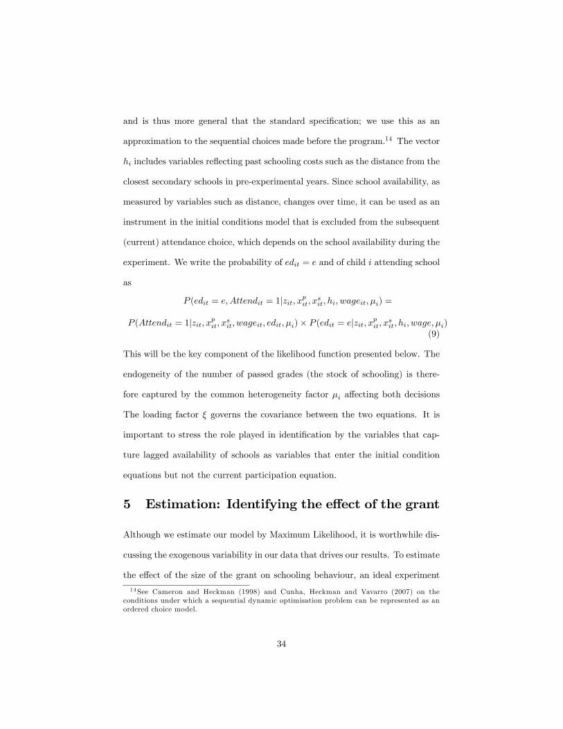
and is thus more general that the standard speci�cation; we use this as an

approximation to the sequential choices made before the program.14 The vector

hi includes variables re�ecting past schooling costs such as the distance from the

closest secondary schools in pre-experimental years: Since school availability, as

measured by variables such as distance, changes over time, it can be used as an

instrument in the initial conditions model that is excluded from the subsequent

(current) attendance choice, which depends on the school availability during the

experiment. We write the probability of edit = e and of child i attending school

as

P (edit = e;Attendit = 1jzit; xpit; xsit; hi; wageit; �i) =

P (Attendit = 1jzit; xpit; xsit; wageit; edit; �i)� P (edit = ejzit; xpit; x

sit; hi; wage; �i)

(9)

This will be the key component of the likelihood function presented below. The

endogeneity of the number of passed grades (the stock of schooling) is there-

fore captured by the common heterogeneity factor �i a¤ecting both decisions

The loading factor � governs the covariance between the two equations. It is

important to stress the role played in identi�cation by the variables that cap-

ture lagged availability of schools as variables that enter the initial condition

equations but not the current participation equation.

5 Estimation: Identifying the e¤ect of the grant

Although we estimate our model by Maximum Likelihood, it is worthwhile dis-

cussing the exogenous variability in our data that drives our results. To estimate

the e¤ect of the size of the grant on schooling behaviour, an ideal experiment

14See Cameron and Heckman (1998) and Cunha, Heckman and Vavarro (2007) on theconditions under which a sequential dynamic optimisation problem can be represented as anordered choice model.

34

would have randomised the potential amounts o¤ered across villages or even

within villages. As it happens they did not. A village either is in the program

or not. Within each PROGRESA village those classi�ed as poor (about 70% of

the population) are eligible for participation in the program. To use the varia-

tion between eligibles, while allowing for the e¤ects of wealth on schooling, we

include a �non-poor�dummy.

The comparison between treatment and control villages and between eligible

and ineligible households within these villages can only identify the e¤ect of the

existence of the grant. However, the amount of the grant varies by the grade of

the child. The fact that children of di¤erent ages attend the same grade o¤ers

a source of variation of the amount that can be used to identify the e¤ect of

the size of the grant. Given the demographic variables included in our model

and given our treatment for initial conditions this variation can be taken as

exogenous. Moreover, the way that the grant amount changes with grade varies

in a nonlinear way, which also helps identify the e¤ect.

Thus the e¤ect of the grant is identi�ed by comparing across treatment and

control villages; by comparing across eligible and ineligible households (having

controlled for being �non-poor�); and by comparing across di¤erent ages within

and between grades. This is our basic model. We also estimate a version of the

model where we allow for di¤erent bahaviour by the ineligible individuals in the

control and treatment villages. We do this by including in our model the �non-

poor�dummy interacted with being in a treatment village. This leaves the other

sources of variation in the grant as identifying information. The motivation for

the introduction of this additional dummy is twofold: �rst, as we documented

above, there were some pre-program di¤erences between the ineligibles in the

35

PROGRESA and the control villages. Second, there may be spillover e¤ects of

the program a¤ecting the behaviour of ineligible individuals, which would mean

that they behave di¤erently from those in the control villages.15

We estimate the model by maximum likelihood.16 To compute the likelihood

function we assume that the distribution of the iid preference shock "it is logistic.

Moreover, we assume that the distribution of unobservables �i is independent of

all observables in the population and approximate it by a discrete distribution

with M points of support sm each with probability pm, all of which need to

be estimated (Heckman and Singer, 1984). The logistic assumption on the "it

allows us to derive a closed form expression for the terms in equation (??).

For the initial condition model, we assume that the residuals of the stock

of education are, conditionally on the unobserved heterogeneity, distributed as

a normal. Therefore, conditional on �i, we have an ordered probit which is

estimated jointly with the schooling decision model.

We should stress that the wage we use in the estimation is the value predicted

by equation 7 (with the exclusion of the Mills ratio). Such an equation accounts

for endogenous selection and takes into account the e¤ect that PROGRESA had

on child wages, so that it imputes a higher values for treatment villages.17

15 see Angelucci and DeGiorgi (2009) fo evidence on spillover e¤ects in consumption. If thedi¤erences were due to GE e¤ects through wages we already account for these.16To achieve the maximum we combine a grid search for the discount factor with a Gauss

Newton method for the rest of the parameters. We did this because often in dynamic modelsthe discount factor is not well determined. However in our case the likelifood function hadplenty of curvature around the optimal value and there was no di¢ culty in identifying theoptimum.17We do not correct the standard errors to take into account that the wage is a generated

regressor.

36

6 Estimation results

In this section, we report the results we obtain estimating di¤erent versions of

the dynamic programming model we discussed above. In particular we will be

discussing three di¤erent versions of the model. The �rst constitutes our basic

model. In the second, we control for the pre-program di¤erence in enrolment

rates among non eligible individuals in treatment and control villages with a

dummy in the speci�cation for schooling costs that identi�es the group of non

eligible boys in treatment villages. Finally, we present the estimates obtained

�tting a version of our model where we impose separability between schooling

and the child wage as discussed in section 4.1 following on from equation 5.

In Tables 3 to 5, we present estimates of the two versions of the basic model

we mentioned above: the �rst column (A) of each table refers to the version that

ignores di¤erences in pre-program school enrollment between treatment and con-

trol villages, while in the second (B) they are accounted for by a dummy for

non-eligible households in treatment localities. This dummy does not have a

signi�cant e¤ect in the initial conditions equation (Table 4) but is signi�cant

in the structural model of educational participation (Table 5). The two de-

gree of freedom likelihood ratio test for excluding this variable has a p-value of

0.8%. However, the parameters hardly change when we move between the two

speci�cations and the substantive implications of the two models are the same.

The third column (C) in the Tables presents estimates of the model obtained

from the control sample only. In this case, the experiment is not used to estimate

the model and all incentive e¤ects are captured by the wage, which acts as the

opportunity cost of education. The purpose of estimating it is to compare the

predictions of a model estimated using the experiment to one that does not and

37

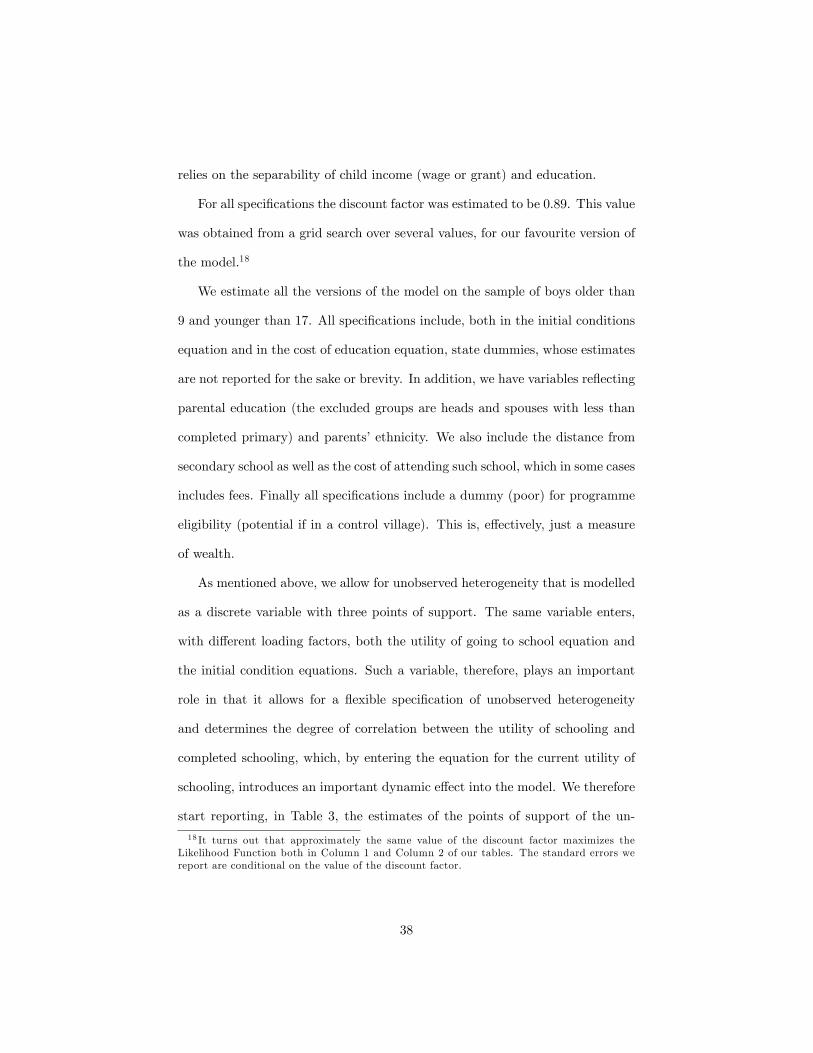
relies on the separability of child income (wage or grant) and education.

For all speci�cations the discount factor was estimated to be 0.89. This value

was obtained from a grid search over several values, for our favourite version of

the model.18

We estimate all the versions of the model on the sample of boys older than

9 and younger than 17. All speci�cations include, both in the initial conditions

equation and in the cost of education equation, state dummies, whose estimates

are not reported for the sake or brevity. In addition, we have variables re�ecting

parental education (the excluded groups are heads and spouses with less than

completed primary) and parents�ethnicity. We also include the distance from

secondary school as well as the cost of attending such school, which in some cases

includes fees. Finally all speci�cations include a dummy (poor) for programme

eligibility (potential if in a control village). This is, e¤ectively, just a measure

of wealth.

As mentioned above, we allow for unobserved heterogeneity that is modelled

as a discrete variable with three points of support. The same variable enters,

with di¤erent loading factors, both the utility of going to school equation and

the initial condition equations. Such a variable, therefore, plays an important

role in that it allows for a �exible speci�cation of unobserved heterogeneity

and determines the degree of correlation between the utility of schooling and

completed schooling, which, by entering the equation for the current utility of

schooling, introduces an important dynamic e¤ect into the model. We therefore

start reporting, in Table 3, the estimates of the points of support of the un-

18 It turns out that approximately the same value of the discount factor maximizes theLikelihood Function both in Column 1 and Column 2 of our tables. The standard errors wereport are conditional on the value of the discount factor.

38

observed heterogeneity terms, and that of the loading factor of the unobserved

heterogeneity terms in the initial condition equation. Three points of support

seemed to be enough to capture the heterogeneity in our sample.

We �rst notice that the results do not vary much across the �rst two spec-

i�cations, while they estimates in Column C are a bit di¤erent. The estimates

in Table 3 reveal that we have three types of children, of which one is very

unlikely to go to school and accounts for roughly 7.6% of the sample. Given

that attendance rates at young ages are above 90%, it is likely that these are

the children that have not been attending primary school and, for some reason,

would be very di¢ cult to attract to school. Another group, which accounts for

about 40.3% of the sample is much more likely to be in school. The largest

group, accounting for 52.1% of the sample, is the middle one. The locations of

the points of support for the model that assumes separability is a bit di¤erent,

but we can still identi�es the three groups we have just discussed.

The loading factor for the �rst two models of the unobserved heterogeneity

term is negative as expected. It implies that individuals more likely to have

completed a higher level of schooling by 1997 are also more likely to be attending

in 1998 due to unobserved factors. Perhaps surprisingly, the loading factor for

the third model is positive.

The initial condition edit is modelled, conditional on the unobserved het-

erogeneity, as an ordered probit with age speci�c cuto¤ points re�ecting the

fact that di¤erent ages will have very di¤erent probabilities to have completed

a certain grade. Indeed, even the number of cuto¤ points is age speci�c, to

allow for the fact that relatively young children could not have completed more

than a certain grade. To save space, we do not report the estimates of the

39

A B CPoint of Support 1 -16.064 -15.622 -4.29

0.991 0.975 2.46Point of Support 2 -19.915 -19.457 -17.62

1.236 1.218 3.144Point of Support 3 -12.003 -11.616 -0.267

0.768 0.758 2.45probability of 1 0.519 0.521 0.49

0.024 0.024 0.032probability of 2 0.405 0.403 0.27

0.025 0.025 0.017probability of 3 0.075 0.076 0.023

- - -load factor for initial condition -0.119 -0.124 0.068

0.023 0.023 0.013Notes: Column A: Eligible dummy only; B: Eligible dummy andnon- Eligible in treatment village dummy. C: Model estimated oncontrol sample only. Asymptotic standard errors in italics

Table 3: The distribution of unobserved heterogeneity

cut-o¤ points. The discrete random term representing unobserved heterogene-

ity is added to the normally distributed random variable of the ordered probit,

e¤ectively yielding a mixture of normals.

In addition to the variables considered in the speci�cation for school utility,

we include among the regressors the presence of a primary and a secondary

school and the distance from the nearest secondary school in 1997. It is im-

portant to stress that these variables are included in the initial condition model

only, in addition to the equivalent variables for 1998, included in both equations.

As discussed above, these 1997 variables, which enter the initial conditions equa-

tion but not the equation for current schooling utility, e¤ectively identify the

dynamic e¤ect of schooling on preferences. It is therefore comforting that they

are strongly signi�cant, even after controlling for the 1998 variables. This indi-

cates that there is enough variability in the availability of school between 1997

40

and 1998. Taking all coe¢ cients together it seems that the most discriminating

variable is the presence of a primary school in 1997.

The results, which do not vary much across the three columns, also make

sense: children living in villages with greater availability of schools in 1997 are

better educated, children of better educated parents have, on average, reached

higher grades, while children of indigenous households have typically completed

fewer grades. Children from poor households have, on average, lower levels of

schooling. As for the state dummies, which are not reported, all the six states

listed seem to have better education outcomes than Guerrero, one of the poorest

states in Mexico, and particularly so Hidalgo and Queretaro.

We now turn to the variables included in the education choice model, re-

ported in the top panel of Table 5. All the variables, except for the grant and

the wage are expressed as determinants of the cost of schooling, so that a pos-

itive sign on a given variable, decreases the probability of currently attending

school. The wage is expressed as a determinant of the utility of work (so given

the positive coe¢ cient, an increase in wages decreases school attendance) and

the grant is a determinant of the utility of schooling, so that an increase in it, in-

creases school attendance. In addition, the coe¢ cient on the grant is expressed

as a ratio to the coe¢ cient on the wage, so that a coe¢ cient of 1 indicates that

a unitary increase in the grant has the same e¤ect on the utility of school as an

increase in the wage has on the utility of work.19

19The wage has been scaled to be interpreted as the earnings corresponding to the periodcovered by the grant. Thus the e¤ects are comparable.

41

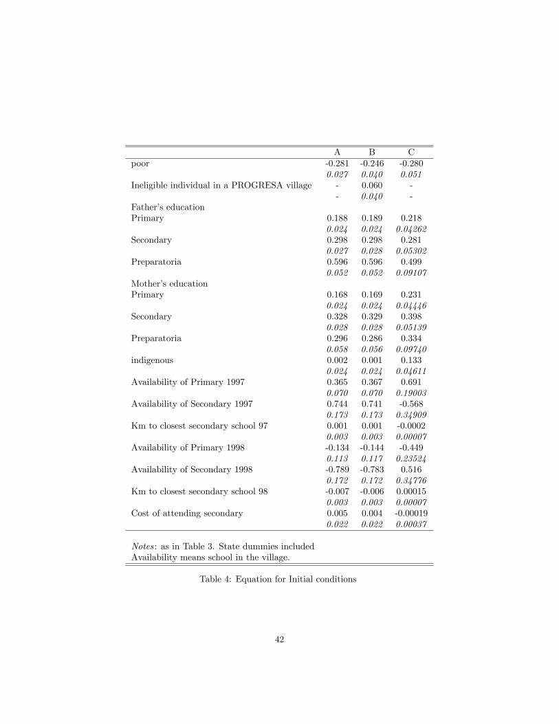
A B Cpoor -0.281 -0.246 -0.280

0.027 0.040 0.051Ineligible individual in a PROGRESA village - 0.060 -

- 0.040 -Father�s educationPrimary 0.188 0.189 0.218

0.024 0.024 0.04262Secondary 0.298 0.298 0.281

0.027 0.028 0.05302Preparatoria 0.596 0.596 0.499

0.052 0.052 0.09107Mother�s educationPrimary 0.168 0.169 0.231

0.024 0.024 0.04446Secondary 0.328 0.329 0.398

0.028 0.028 0.05139Preparatoria 0.296 0.286 0.334

0.058 0.056 0.09740indigenous 0.002 0.001 0.133

0.024 0.024 0.04611Availability of Primary 1997 0.365 0.367 0.691

0.070 0.070 0.19003Availability of Secondary 1997 0.744 0.741 -0.568

0.173 0.173 0.34909Km to closest secondary school 97 0.001 0.001 -0.0002

0.003 0.003 0.00007Availability of Primary 1998 -0.134 -0.144 -0.449

0.113 0.117 0.23524Availability of Secondary 1998 -0.789 -0.783 0.516

0.172 0.172 0.34776Km to closest secondary school 98 -0.007 -0.006 0.00015

0.003 0.003 0.00007Cost of attending secondary 0.005 0.004 -0.00019

0.022 0.022 0.00037

Notes: as in Table 3. State dummies includedAvailability means school in the village.

Table 4: Equation for Initial conditions

42

A B Cwage 0.103 0.110 0.357

0.033 0.033 0.100PROGRESA Grant 4.154 3.869 -

1.386 1.036 -parameter in terminal function ln(�1) 5.798 5.797 6.59

0.099 0.099 0.175parameter in terminal function ln(�2) -1.104 -1.103 -1.62

0.020 0.020 0.089Poor 0.159 -0.128 0.431

0.118 0.164 0.274Ineligible individual in a PROGRESA village -0.492

0.198Father�s Education - Default is less than primaryPrimary -0.131 -0.133 -0.486

0.093 0.092 0.217Secondary -0.271 -0.267 -0.959

0.113 0.112 0.261Preparatoria -0.751 -0.735 -2.176

0.253 0.250 0.558Mother�s Education - Default is less than primaryPrimary -0.136 -0.131 -0.870

0.096 0.096 0.233Secondary -0.137 -0.129 -1.119

0.113 0.113 0.254Preparatoria -0.920 -0.893 -2.158

0.284 0.283 0.645indigenous -0.605 -0.591 -1.018

0.107 0.107 0.241Availability of Primary 1998 2.734 2.744 3.092

0.220 0.219 0.499Availability of Secondary 1998 -0.160 -0.189 0.789

0.152 0.152 0.425Km to closest secondary school 98 0.001 0.001 0.00078

0.004 0.004 0.00014Cost of attending secondary 0.005 0.005 0.013

0.001 0.001 0.0033Age 2.772 2.758 2.903

0.180 0.180 0.354Prior Years of education -2.995 -2.996 -3.621

0.214 0.214 0.621Discount rate 0.89 0.89 0.975log-Likelihood -26,676.676 -26,672.064 -8862.34

� = State dummies includedNotes as in Table 3.

Table 5: Parameter estimates for the Education choice model43

From a policy perspective, the key parameters of the model are the wage co-

e¢ cient and the coe¢ cient on the grant itself. An increase in the wage decreases

the probability of attending school. On average, the e¤ect of reducing the wage

by 44% (which would roughly give a reduction similar to the average grant to

bene�ciaries) increases the probability of attending school by 2.1%. This e¤ect

cannot be inferred directly from the value of the parameter alone and has been

obtained from the simulations of the model that we discuss in detail below. The

wage e¤ect is higher when we estimate the model on the control villages alone.

The di¤erence between the wage coe¢ cient in column A and C is signi�cant

and has a t-value of 3.25 based on a Durbin-Wu-Hausman type test.

The value of the grant varies by treatment and control villages (where of

course it is zero) and by grade the child could be attending.20 As mentioned

above, the coe¢ cient of the grant is expressed as a fraction of the wage coef-

�cient. The values of about 4 for this coe¢ cient reported in Table 5 indicates

that the e¤ect of the grant on school attendance is considerably larger than the

e¤ect of the wage.21 Such an assumption is easily rejected by a likelihood ratio

test.22 . As discussed earlier this test rejects the hypothesis that education and

consumption can be taken to be separable and implies the importance of having

experimental information to assess the impact of policy in this case.

In terms of background characteristics, belonging to a household with less

educated parents leads to lower attendance. This may be a re�ection of liq-

uidity constraints or of di¤erent costs of schooling. Perhaps surprisingly, the

20As mentioned above, in secondary school, the grant is also higher for girls than for boys.However, as we only estimate the model for the latter, we do not exploit this variation.21The non-linearity of the model implies that the e¤ect of enrolment is not 3 or 4 times

larger than the e¤ect of enrolment of the wage.22The likelihood ratio test is 30 and is distributed �2

(1)under the null. Since this hypothesis

relates to a non-linear restriction and subject to a variety of di¤erent normalisations the Waldtest is not appropriate. See Gregory and Veall (1985).

44

coe¢ cient on poor (eligible) households is not signi�cantly di¤erent from zero,

while that on indigenous households indicates that, ceteris paribus, they are

more likely to send their children to school. The states that exhibit the higher

costs are Queretaro and Puebla, followed by San Luis Potosi and Michoacan,

while Veracruz and Guerrero are the cheapest. The costs of attending secondary

measured in either distance (since many secondary schools are located in neigh-

bouring village) or in terms of money have a signi�cant and negative e¤ect on

attendance.

Both age and grade have a very important e¤ect on the cost of schooling, age

increasing and grade decreasing it. The coe¢ cient on age is the way in which

the model �ts the decline in enrolment rates by age across both treatment and

control villages. The e¤ect on the grade captures the dynamics of the model

and, as we discussed, is identi�ed by the presence of lagged supply of school

infrastructure. We �nd a very strong e¤ect of state dependence despite the

fact that we include age as one of the explanatory variables. The pre-existing

level of education is a critical determinant of choice, with increased levels of

education having a substantially positive e¤ect on further participation. This

is of course an important point since it provides an additional mechanism by

which the subsidy may increase educational participation and is likely to be key

for simulating alternative policies. It also implies di¤erent e¤ects depending on

the amount of prior educational participation. The likelihood ratio test for the

null that past education does not matter has a p-value of zero (the likelihood

ratio statistic is 300). Moreover, eliminating habits leads to an overprediction

of the program e¤ects.

As we discussed above, we have scant information on the returns to educa-

45

tion, so that we include the returns to education among the parameters to be

inferred from the di¤erential attendance rates in school. It is therefore impor-

tant to check what are the returns to education implied by this model. When

we compute the return to education implied by the coe¢ cients on the terminal

value function, we obtain an estimate of the average return to education of 5%

per year, maybe a bit low in the Mexican context, but above the average return

to education observed in our villages.23

Cost variables have the expected sign and are signi�cant. For instance, an in-

crease in the distance from the nearest secondary school, signi�cantly decreases

the probability of attending school. Likewise for an increase in the average cost

of attending secondary school. As several of the children in our sample are still

attending primary school we also tried to include variables re�ecting the cost

and availability of primary schools, but we could not identify any signi�cant

e¤ect.

7 Simulations

The model is complex and non linear. To check how the various speci�cations

of the model are able to predict the impact of the grant and to quantify the

e¤ect of the main variables of interest from a policy point of view we present the

results of simulations of various versions of the model. We start. by comparing

the impacts predicted by the di¤erent versions of the model with the impacts

of PROGRESA as estimated by comparing enrolment rates in treatment and

control localities, as we have done in Section 3. We then study changes to the

program and alternative policies.

23The return is calculated as r = @VTVT @ed

where VT = V (edi;18) and where the parameters�1and �2 are given in their logs in column 3 of Table 5.

46

7.1 Predicting the impact of PROGRESA

To check how our basic model predicts the impact of the program, we simulate

the behaviour of the children in our sample under two di¤erent scenarios. The

�rst correspond to the actual data and includes, in the treatment communities,

the grant. It should be stressed that, in these communities, the grant is assumed

to be permanent. The second is a scenario in which, counterfactually, we set the

grant equal to zero. We then compute the probability of school enrolment of

eligible boys in treatment communities under the two scenarios, average these

probabilities for di¤erent age groups and interpret the di¤erent in probabilities

as the impact of the program.

When removing (counterfactually) the grant from treatment areas, we com-

pute two predictions. In one case we keep children wages constant across com-

parisons, assuming that is that the program did not a¤ect wages. This is what

one would calculate based on a partial equilibrium model estimated on the con-

trols only. We label this �e¤ect of Grant - No GE�. In a second calculation,

when we remove the grant we also adjust wages downwards based on our esti-

mates of the impact of the grant on wages. We label this �e¤ect of Grant - GE�.

To these results, plotted in Figure 1. ,we juxtapose the experimental impacts

discussed in Section 3. , which is the dotted line.

In column C of Tables 3 to 5, we presented estimates of a model estimated on

the sample of control villages only. We have already demonstrated that the e¤ect

of the grant is not equivalent to a corresponding reduction of the wage, which is

the opportunity cost of education. We interpret this as a rejection of separability

of child income and education24 in a model where income pooling is not imposed

24See Browning and Meghir (1991).

47

(see estimates in Column C of the results tables). This in itself implies that a

model estimated without the experimental variation cannot accurately predict

the e¤ects of the experiment on educational participation. In addition to show

how our model predicts the impact of the program, we also want to show the

extent to which the rejection of the simpler model that assumes separability

between consumption and child labour, is a quantitatively important issue.

The left hand side panel in Figure 1 relates to our basic model estimated both

on the treatment and control samples. As we plot the di¤erence in probabilities

only for eligible children, and as the estimates of most coe¢ cients do not change

much between the two versions of the model (with and without the non-eligible

treatment village dummies), not surprisingly the age pro�le of the impacts look

very similar. Therefore, in the Figure, we only report one of them.

The right hand side panel in Figure 1. reports the impacts predicted by

the model estimated only on control villages with the separability assumption

imposed. In this case, the impact of the grant is derived from the coe¢ cient on

the wage.

Not surprisingly, the average e¤ect of the treatment (estimated experimen-

tally at 0.05) is predicted quite accurately by the model at 0.047. Moreover, the

model predicts reasonably well the inverted U-shape of the impact. Estimat-

ing the model based on the controls only we obtain an average e¤ect of 0.031.

However, what is more interesting is to consider the age pattern of the e¤ect.

Consider �rst the comparisons that keep wages constant. The age pattern

is very similar to the experimental one, except that the model misses the 14%

peak e¤ect at age 14 and compensates with higher e¤ects around these ages.

The failure of the model to replicate the peak is unsurprising given the simple

48

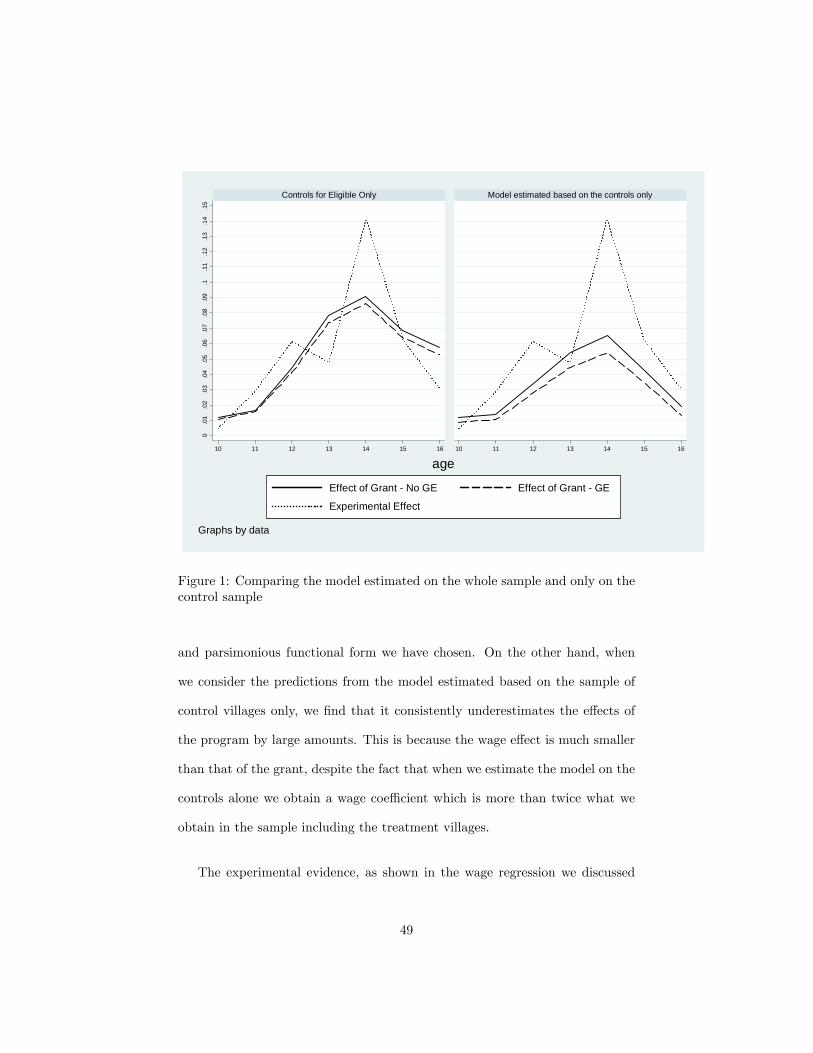
0.0

1.0

2.0

3.0

4.0

5.0

6.0

7.0

8.0

9.1

.11

.12

.13

.14

.15

10 11 12 13 14 15 16 10 11 12 13 14 15 16

Controls for Eligible Only Model estimated based on the controls only

Effect of Grant ­ No GE Effect of Grant ­ GE

Experimental Effect

age

Graphs by data

Figure 1: Comparing the model estimated on the whole sample and only on thecontrol sample

and parsimonious functional form we have chosen. On the other hand, when

we consider the predictions from the model estimated based on the sample of

control villages only, we �nd that it consistently underestimates the e¤ects of

the program by large amounts. This is because the wage e¤ect is much smaller

than that of the grant, despite the fact that when we estimate the model on the

controls alone we obtain a wage coe¢ cient which is more than twice what we

obtain in the sample including the treatment villages.

The experimental evidence, as shown in the wage regression we discussed

49

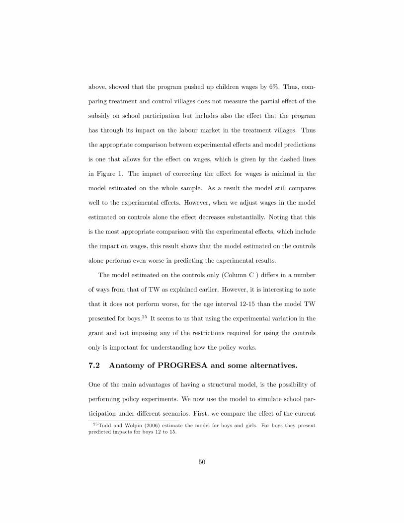
above, showed that the program pushed up children wages by 6%. Thus, com-

paring treatment and control villages does not measure the partial e¤ect of the

subsidy on school participation but includes also the e¤ect that the program

has through its impact on the labour market in the treatment villages. Thus

the appropriate comparison between experimental e¤ects and model predictions

is one that allows for the e¤ect on wages, which is given by the dashed lines

in Figure 1. The impact of correcting the e¤ect for wages is minimal in the

model estimated on the whole sample. As a result the model still compares

well to the experimental e¤ects. However, when we adjust wages in the model

estimated on controls alone the e¤ect decreases substantially. Noting that this

is the most appropriate comparison with the experimental e¤ects, which include

the impact on wages, this result shows that the model estimated on the controls

alone performs even worse in predicting the experimental results.

The model estimated on the controls only (Column C ) di¤ers in a number

of ways from that of TW as explained earlier. However, it is interesting to note

that it does not perform worse, for the age interval 12-15 than the model TW

presented for boys.25 It seems to us that using the experimental variation in the

grant and not imposing any of the restrictions required for using the controls

only is important for understanding how the policy works.

7.2 Anatomy of PROGRESA and some alternatives.

One of the main advantages of having a structural model, is the possibility of

performing policy experiments. We now use the model to simulate school par-

ticipation under di¤erent scenarios. First, we compare the e¤ect of the current

25Todd and Wolpin (2006) estimate the model for boys and girls. For boys they presentpredicted impacts for boys 12 to 15.

50

program with that of a similar program that di¤ers in the way in which the

grant varies with the grade attended.

The aim of this exercise is to compare the impact of the current grant, as

predicted by our model, to the impact that is obtained when the structure of

the grant is changed so as to target the program to those in the most responsive

ages. In particular, we focus on a �balanced budget�reform of the program. That

is, we increase the grant for children above grade 6 and set it to zero for children

below that grade. The increase for the older children is calibrated so that, taking

into account the response of children schooling choices to the change, the overall

cost of the program is left unchanged (at least for our sample).

We plot the result of this exercise in Figure 2 where again we show the

results with no wage adjustment (continuous line) and with a GE adjustment.

Performing the GE adjustment is now a bit more complicated than in the

previous exercise. The amount by which children wages would change with the

counterfactual grant structure has to be extrapolated. We do that by using the

elasticities discussed in Section 4.5.

The graph shows that by targeting the grant to the older children we can

almost double the impact relative to the predicted e¤ect from the model shown

in the left panel of Figure 1. This occurs with no e¤ect on the school participa-

tion of the younger primary age children. This is not surprising since the grant

hardly changes their behavior in the �rst place because almost all children go

to school below grade 6, making it an unconditional transfer for that age group.

The overall resources targeted to families with children do not change with this

reform, but the incentive structure does.

This change to the grant structure seems to suggest a modi�cation to the

51

program that would much improve its ability to increase enrolment rates. This

is particularly important because the modi�ed program costs, in the steady

state, the same amount as the current one. From the point of view of the

households, notice that they receive the same amount of resources over time:

what changes is when they receive them. If households can borrow against the

future grant, then the only e¤ect of this reform is to improve incentives for

school participation at later ages. If on the other hand families are liquidity

constrained the trade-o¤ may be more serious, particularly if the grant at a

younger age a¤ects nutrition or other child inputs.26 Attanasio and Rubio-

Codina (2008) show that the impact of the PROGRESA grant on a variety of

nutritional outcomes for very young children does not depend on whether they

have primary school age siblings. This might be an indication that a change in

the grant structure as the one describe might not have large negative e¤ects.

More recently, the Mexican government is piloting two versions of the program

in which primary school grants are eliminated and secondary school grants are

increased.

We next consider a number of alternative experiments. In particular we

consider the e¤ect of decreasing the wage by an amount equivalent to the grant;

the e¤ect of distance to school; and the impact of the grant on children with

low cost of education. All three experiments are summarized in �gure 3. In all

cases we use the model A in the tables. No grant is our baseline.

First we decrease the wage by an amount equivalent to the grant.27 We

see that the e¤ect of the wage is estimated to be much lower than the grant;

26Attanasio and Kaufman (2009) show that for the Oportunidades/PROGRESA popula-tion, liquidity constraints can be important.27The reduction is proportional so as to give an average amount equivalent to the grant.

The grant however is additive. So we would not expect the e¤ects of the wage to be distributedequally because the wage varies with age much more steeply than the grant.

52

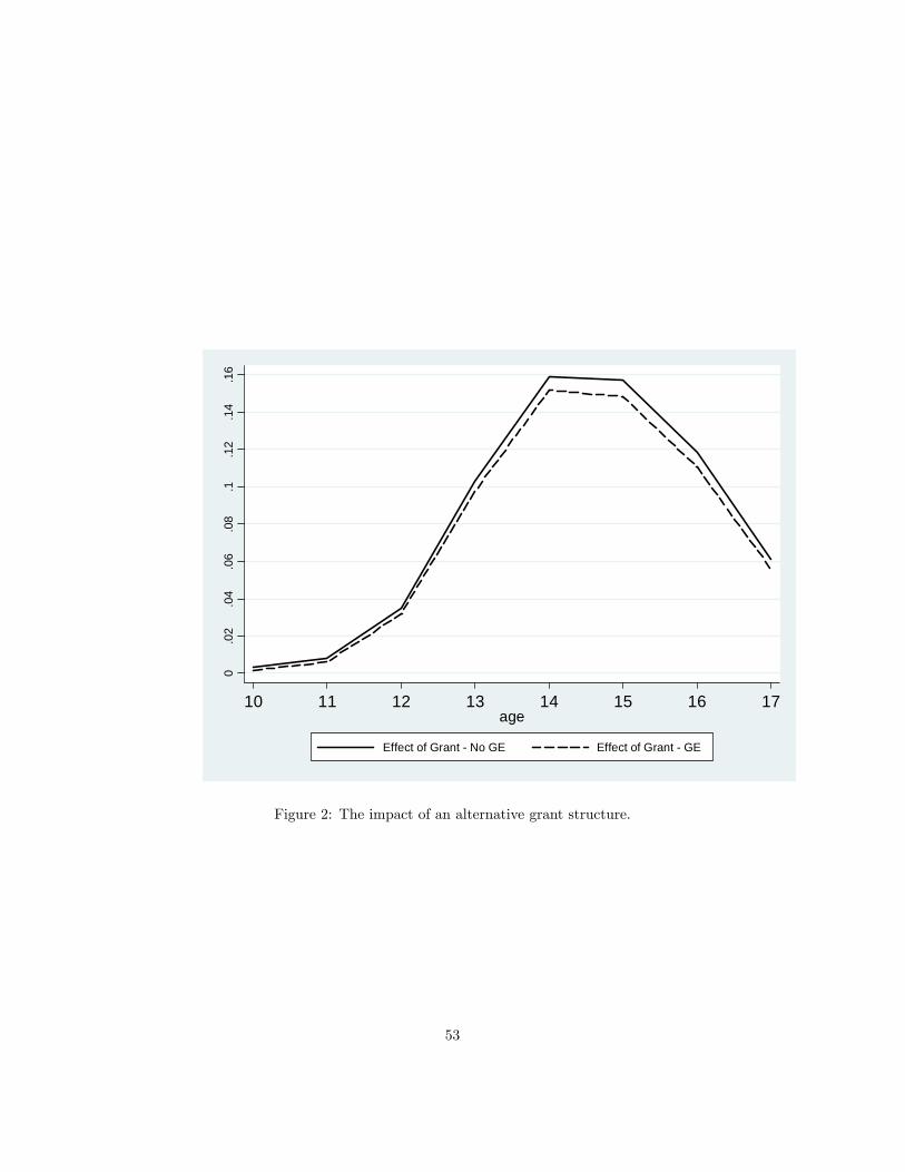
0.0

2.0

4.0

6.0

8.1

.12

.14

.16

10 11 12 13 14 15 16 17age

Effect of Grant ­ No GE Effect of Grant ­ GE

Figure 2: The impact of an alternative grant structure.

53

0.0

1.0

2.0

3.0

4.0

5.0

6.0

7.0

8.0

9.1

.11

10 11 12 13 14 15 16 17age

Effect of wage reduction Effect of reducing distance to School

Effect on low cost children

Figure 3: The impact of alternative policy experiments

54

for example at age 15 the incentive e¤ect is less than half the one in Figure ??.

This evidence re-emphasises the point already made, that the experimental data

provides information on behaviour that may not be available through observed

data.

In the next experiment we demonstrate the e¤ects of a potential school

building program that would reduce the distance of secondary schools to no

more than 3 km. We consider this because it could constitute an alternative

policy to subsidizing participation (although we do not claim that this policy is

equivalent in terms of cost or in terms of other bene�ts such as better nutrition

and its impact). According to our parameter estimates the e¤ect is modest as

it would increase participation by just below 2 percentage points at age 15.

Finally in order to demonstrate the potential importance of targeting, we

show the e¤ects of the policy on individuals with �low cost�of schooling; i.e. we

evaluate the e¤ect at the point of support of the unobserved heterogeneity with

the highest school participation. As shown in the graph for these individuals

there is no e¤ect of the program before age 14. Beyond that the e¤ects are

higher than average. Conversely, for the high cost of schooling individuals (not

shown) the e¤ects are higher than average at younger ages and lower later.

8 Conclusions

In this paper we demonstrate the power of using an economic model to analyse

data from a major social experiment, namely PROGRESA in Mexico. Con-

versely, we also show the usefulness of using experimental data to estimate a

structural economic model. The welfare program we consider was originally

applied to rural Mexico and aimed, among other things, at increasing school

55

enrolment rates among poor children.

We start by showing some of the e¤ects of this program on school participa-

tion. As the program was randomised across villages, inducing truly exogenous

variation in the incentives to attend school, by o¤ering a subsidy for atten-

dance, estimation of its impact is relatively straightforward. After presenting

some evidence based on simple treatment/control comparisons, we argue that

many questions are left unanswered by this type of techniques and propose the

use of a structural model.

By interpreting the data through the viewpoint of a dynamic model one can

investigate how the impacts of the program would be di¤erent if one were to

change some of its parameters. In particular, we analyze what would happen to

the program�s impact on enrolment by changing the structure of the grants with

age. This type of analysis is instrumental to the design of e¤ective interventions

and cannot be performed without a well speci�ed behavioural model. We can

also compare the impacts of the program with alternative policies, such as a

program that would reduce the distance of the households in our sample from

the nearest secondary school. Therefore we show that only through this kind

of modelling approach is it possible to answer questions that are more general

than the speci�c focus of the evaluation.

But this is not a one way street: we also argue that the use of the experimen-

tal data and the genuine exogenous variation it induces, allows us to identify

models that are richer than those that could be identi�ed based on standard

observational data. In our speci�c context, we show that, although the pro-

gram operates by changing the relative price of education and its opportunity

cost, the economic incentives it provides are much larger than those provided

56

by changes in children wages. This is important from a policy point of view,

but also for modelling if one notes that without the experimental variation our

model could not be estimated. Our approach provides a rich set of results and

at the same time points to the importance of the interaction between economic

models and social experiments for the purposes of evaluation and understanding

behaviour.

The experimental design of the evaluation data, where the program was ran-

domized across communities, and the fact that the localities in the sample are

relatively isolated, allows one to estimate the general equilibrium e¤ect that

the program has on children wages. Having estimated these e¤ects, we incor-

porate this additional channel in our structural model, both at the estimation

stage (where our estimated wage equation incorporates the GE e¤ects) and in

performing the simulation of alternative interventions.

The model we estimate �ts the data well and predicts impacts that match

the results obtained by the experimental evaluation closely. They indicate that

the program is quite e¤ective in increasing the enrolment of children at the end

of their primary education, a fact that has been noticed in several evaluations

of conditional cash transfers in Latin America. On the other hand, the program

does not have a big impact on children of primary school age, partly because

enrolment rates for these children are already quite high.

We identify relatively large general equilibrium e¤ects of the program on

child wages: in the treatment localities child wages are about 6% higher than

in control localities. Remarkably, this fact had not been noticed in the large

empirical literature on PROGRESA. Although these e¤ects and the impact

that the program is observed to have on school enrolment (and child labour

57

supply) imply relatively large elasticities of wages to changes in enrolment, the

attenuating e¤ect on the impact of the grant is not large.

The heterogeneity of the program impacts by age has suggested the possibil-

ity of changing the structure of the grant, reducing or eliminating the primary

school grant and increasing the size of the grant for secondary school. This

proposal, that has been considered in urban Mexico and in Colombia, can be

analyzed with the help of our structural model. The simulations we perform

indicate that the e¤ect on school participation could be much improved by of-

fering more resources to older children and less to relatively younger one. By

taking into account behavioural responses, we simulate changes to the program

that result in the same amount of resources spent by the program and yet obtain

much larger impacts on school enrolment of older children.

Some words of caution are obviously in order when considering the results

of our simulations. It should be pointed out, for instance, that our model is

silent as to the e¤ect of the grant on other dimensions of child development.

Since most young children go to school anyway, the grant for them is e¤ectively

unconditional and can have other e¤ect such as on their nutrition and result-

ing physical and cognitive development. Although the reformulated grant could

transfer the same resources to the families whose children continued school at-

tendance, albeit with di¤erent timing the e¤ects on these other dimensions we

do not model could be di¤erent in the presence of liquidity constraints; moreover

fewer resources would end up with those who despite the increased grant drop

out of school anyway. Nevertheless,our results imply that in terms of school

participation, changing the age structure of the grant would achieve di¤erent

results.

58

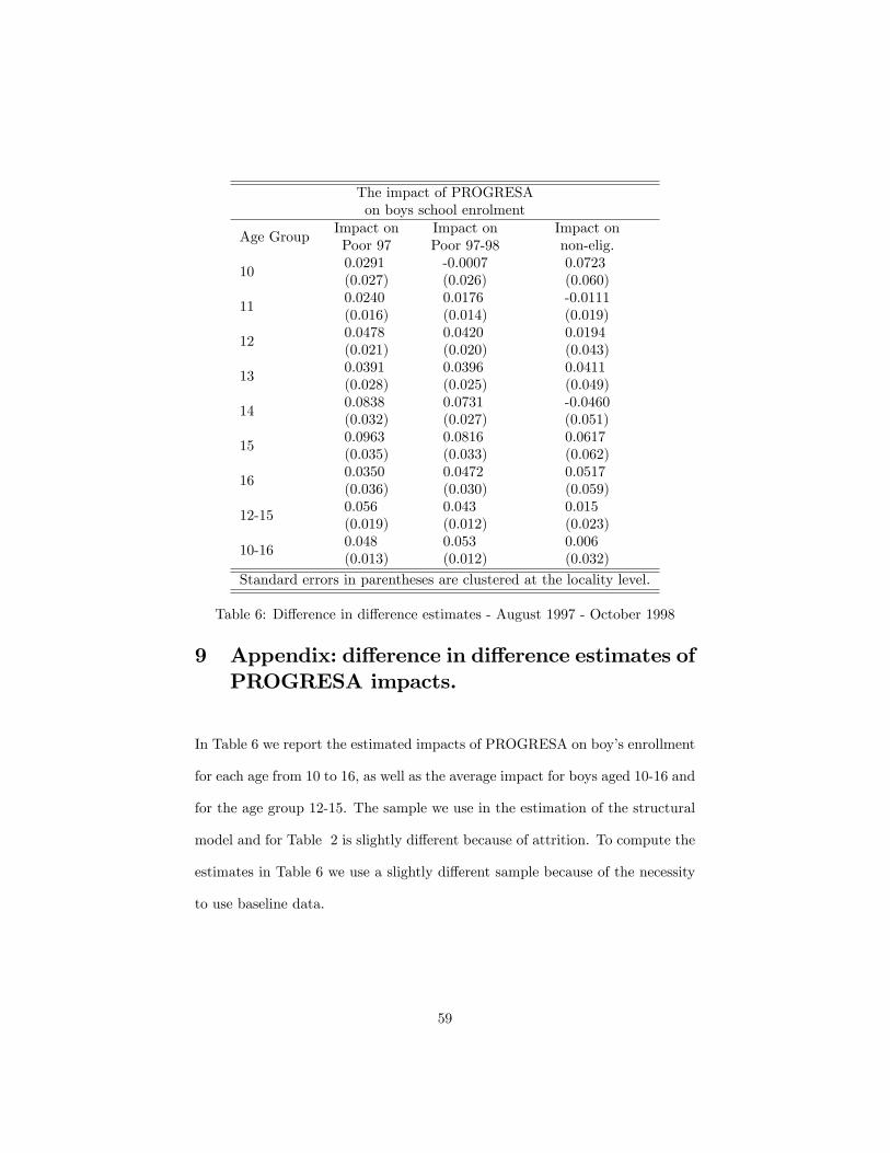
The impact of PROGRESAon boys school enrolment

Age GroupImpact onPoor 97

Impact onPoor 97-98

Impact onnon-elig.

100.0291(0.027)

-0.0007(0.026)

0.0723(0.060)

110.0240(0.016)

0.0176(0.014)

-0.0111(0.019)

120.0478(0.021)

0.0420(0.020)

0.0194(0.043)

130.0391(0.028)

0.0396(0.025)

0.0411(0.049)

140.0838(0.032)

0.0731(0.027)

-0.0460(0.051)

150.0963(0.035)

0.0816(0.033)

0.0617(0.062)

160.0350(0.036)

0.0472(0.030)

0.0517(0.059)

12-150.056(0.019)

0.043(0.012)

0.015(0.023)

10-160.048(0.013)

0.053(0.012)

0.006(0.032)

Standard errors in parentheses are clustered at the locality level.

Table 6: Di¤erence in di¤erence estimates - August 1997 - October 1998

9 Appendix: di¤erence in di¤erence estimates ofPROGRESA impacts.

In Table 6 we report the estimated impacts of PROGRESA on boy�s enrollment

for each age from 10 to 16, as well as the average impact for boys aged 10-16 and

for the age group 12-15. The sample we use in the estimation of the structural

model and for Table 2 is slightly di¤erent because of attrition. To compute the

estimates in Table 6 we use a slightly di¤erent sample because of the necessity

to use baseline data.

59

10 References

Angelucci, M and G. DeGiorgi (2009) �Indirect E¤ects of an Aid Program: TheCase of Progresa and Consumption�American Economic Review, 2009, 99(1),486-508.Attanasio, O.P. and K.M. Kaufmann (2009) �Educational Choices, Sub-

jective Expectations, and Credit Constraints� NBER Working Papers 15087,National Bureau of Economic Research.Attanasio, O. and M. Rubio-Codina (2008): �Revaluatig Conditional Cash

Transfers: Is the Oportunidades Primary School Stipend Necessary?�, IFSMimeoBehrman, J. (1999): �Education, Health and Demography in Latin America

Around the End of the Century: What Do We Know? What Questions ShouldBe Explored?�, IADB Mimeo.Behrman, J., Duryea, S. and M. Székely (1999):�Schooling Investments and

Aggregate Conditions: A Household Survey-Based Approach for Latin Americaand the Caribbean�, OCE Working Paper No 407, IADB, Washington:http://www.iadb.org/res/publications/pub�les/pubWP-407.pdf.Behrman, J., Duryea, S. and M. Székely (2000): �Households and Economic

Growth in Latin America and the Caribbean�, GDN, Mimeo.Behrman, J. and P. Todd (1999); �Randomness in the Experimental Samples

of PROGRESA (Education,Health, and Nutrition Program)�, IFPRI. down-loadable from:http://www.ifpri.org/themes/PROGRESA/pdf/BehrmanTodd_random.pdf

.Blundell Richard, Pierre Andre Chiappori, Costas Meghir and (2005) Col-

lective Labour Supply with Children Journal of Political Economy, Volume 113,Number 6, December 2005Blundell Richard, Pierre Andre Chiappori, Thierry Magnac and Costas

Meghir and (2007 ) Collective Labour Supply: Heterogeneity and Non-Participation,Review of Economic Studies (2007) 74, 417�445Browning, Martin & Meghir, Costas (1991) "The E¤ects of Male and Female

Labor Supply on Commodity Demands," Econometrica, vol. 59(4), pages 925-51, July.Burtless, Gary and Jerry A. Hausman (1978) �The E¤ect of Taxation on

Labor Supply: Evaluating the Gary Negative Income Tax Experiment� TheJournal of Political Economy, Vol. 86, No. 6 (Dec., 1978), pp. 1103-1130Published by: The University of Chicago PressCameron, Stephen V. and James J. Heckman (1998) �Life Cycle Schooling

and Dynamic Selection Bias: Models and Evidence for Five Cohorts of AmericanMales�The Journal of Political Economy, Vol. 106, No. 2 (Apr., 1998), pp.262-333Cunha, Flavio, James. J. Heckman and Salvador Navarro (2007)�The Iden-

ti�cation and Economic Content of Ordered Choice Models with StochasticThresholds�International Economic Review Vol. 48, No. 4, November 2007

60

Dearden, L. C. Emmerson, C. Frayne and C. Meghir (2008) �Can EducationSubsidies stop School Drop-outs? An evaluation of Education MaintenanceAllowances in England�, IFS discussion paper forthcoming Journal of HumanResources.Gregory, A.W. and M.R. Veall (1985), "Formulating Wald Tests of Nonlinear

Restrictions", Econometrica, vol. 54, no. 6, November (1985), 1465-1468.Heckman, J.J. (1979) �Sample Selection Bias as a Speci�cation Error",

EconometricaHeckman, J.J and B. Singer (1984) �A Method for Minimizing the Impact of

Distributional Assumptions in Econometric Models for Duration Data�Econo-metrica Vol. 52, No. 2 (Mar., 1984), pp. 271-320Mo¢ tt Robert A. (1979)�The Labor Supply Response in the Gary Experi-

ment�The Journal of Human Resources, Vol. 14, No. 4 (Autumn, 1979), pp.477-487Meghir, C. and L. Pistaferri (2004) �Income Variance Dynamics and Het-

erogeneity�Econometrica, January 2004 pp 1-32Orcutt, G. H., and A. G. Orcutt (1968) Incentive and Disincentive Experi-

mentation for Income Maintenance Policy Purposes," American Economic Re-view, 58, 754-772.Rawlings, L. (2004): �A New Approach to Social Assistance: Latin Amer-

ica�s Experience with Conditional Cash Transfer Programs�, World Bank SocialProtection Discussion Paper No 0416.Schultz, T.P. (2003): �School Subsidies for the Poor: Evaluating the Mexican

PROGRESA Poverty Program�, Journal of Development Economics,Skou�as, E. (2001): �PROGRESA and its Impacts on the Human Capital

and Welfare of Households in Rural Mexico: A Synthesis of the Results of anEvaluation by IFPRI.�, IFPRI, downloadable from:http://www.ifpri.org/themes/PROGRESA/pdf/Skou�as_�nalsyn.pdfThomas, Duncan (1990) �Intra-Household Resource Allocation: An Infer-

ential Approach�, The Journal of Human Resources, Vol. 25, No. 4 (Autumn,1990), pp. 635-664Todd , P. and K. Wolpin (2006): �Using Experimental Data to Validate

a Dynamic Behavioral Model of Child Schooling and Fertility: Assessing theImpact of a School Subsidy Program in Mexico�, American Economic Review,96(5): 1384�1417

61