comparison of taguchi method and robust design ... · comparison of taguchi method and robust...

Comparison of Taguchi Method and Robust DesignOptimization (RDO)

- by application of a functional adaptive simulation model for the

robust product-optimization of an adjuster unit -

Stefan Kemmler1∗ & Alexander Fuchs2 & Tobias Leopold2 & Bernd Bertsche1

1 Institute of Machine Components (IMA), University of Stuttgart

2 Knorr-Bremse Systeme fur Nutzfahrzeuge GmbH

Abstract

Current research and development have been trending towards approaches basedon simulation and virtual testing. Industrial development processes for complexproducts employ optimization methods to ensure results are close to reality, simul-taneously minimizing required resources. The results of virtual testing are optimizedin accordance with requirements using optimization techniques. Robust Design Op-timization (RDO) is one established approach to optimization. RDO is based onthe identification of an optimal parameter set which includes a small variance of thetarget value as a constraint.Under most circumstances, this approach does not involve separate optimization ofthe target value and target variance. However, the basic strategy of the optimizationapproach developed by Taguchi is to first optimize the parameter sets for the targetvalue and then optimize and minimize the target variance.According to an application example , the benefit of Taguchi’s approach (TM) isthat it facilitates the identification of an optimal parameter set of nominal valuesfor technical feasibility and possible manufacturing. If an optimal parameter set isdetermined, the variance can be minimized under consideration of process parame-ters.This paper examines and discusses the differences between and shared characteri-stics of the robust optimization methods TM and RDO, and discusses their shortco-mings. In order to provide a better illustration, this paper explains and applies bothmethods using an adjuster unit of a commercial vehicle braking system. A simula-tion model is developed including an appropriate workflow by applying optiSLang-modules.

Keywords: Robust Design, SMAR2T, Robust Design Optimization, Reliability-basedDesign Optimization, Taguchi Method, Adjuster Unit

∗Contact: Dipl.-Ing. Stefan Kemmler, Institute of Machine Components (IMA), University of Stutt-gart, Pfaffenwaldring 9, D-70569 Stuttgart, E-Mail: [email protected]

1

1 Introduction

Faced with rapid product development and increasing customer requirements, it is notalways possible to achieve required product quality. When a product does not meet quali-ty standards, this can have major consequences, such as a loss of company image and/oruncontrollable declines in sales. There are many examples of consumer product recalls,which spread immediately through various media channels.The demand for robust and reliable products is increasing to ensure these requirementsare met,. Products must be as insensitive as possible against both external (e.g. environ-mental conditions) and internal noise factors (e.g. component deviations). One approachto designing such products is the Robust Design Method (RDM), whose aim is to createproducts insensitive to uncontrollable variations (noise factors). Reliability engineeringmethods are deployed in order to provide the desired product functionality throughoutthe required service life.. The multidomain method SMAR2T (Kemmler and Bertsche(2014a), Kemmler and Bertsche (2014b), Kemmler et al. (2014), Kemmler et al. (2015))is used to design such robust and reliable products.Virtual product development is an additional supportive indicator , specifically in simu-lation technology during the product development process (PDP). Virtual product deve-lopment can predict the behaviour of products or their functions early on in the PDP,taking into account a large number of varying factors and resulting in saved resources.Simulation tools are being used more and more frequently in industry; one of these is thefinite element method (FEM). Based on the simulation results provided by this method,developers can increase and optimize the robustness of products using the RD methodsRobust Design Optimization (RDO) or the Taguchi Method (TM).One simulation-based approach both in RDO and TM is the creation of Meta models,which are created from multiple design points as a result of the FEM using mathematicalregression models describing the relationship between input and output characteristics.These regression models can allow developers to describe robustness and correspondingoptimal parameter settings simultaneously. However, a production-oriented design mustbe determined and validated using specific and real experiments. This paper presents thefundamental characteristics of both RD methods, then applies them to a concrete exampleof an adjusting unit for commercial vehicle braking systems. Finally, as a result, it derivesa universal workflow.

2 Differences and similarities between Robust Design

Optimization and the Taguchi Method

According to Park et al. (2006) there are three basic methods of Robust Design: the Axio-matic Design (AD) (Suh (2001)), the Taguchi Method (TM) (Taguchi, G. et al. (2005))and the new discipline of Robust Design Optimization (RDO). In general AD describes thecomplexity of a system and its relation between Customer Requirements (CR), FunctionalRequirements (FR), Design Parameters (DP) and Process Variables (PV). Furthermore,AD is used in the early concept phase after SMAR2T. Therefore, this paper will onlyexamine and discuss the differences and similarities between TM and RDO.

12. Weimar Optimization and Stochastic Days – 5.-6. November 2015 2

2.1 Taguchi Method

Japanese electrical engineer Genichi Taguchi has developed an attractive tool for industry.The Taguchi Method optimizes the product development process to ensure that robustproducts of high quality can be developed at a low cost. The method aims to minimizevariation of the quality characteristics of products.

2.1.1 Approach

Like RDO, the control and noise factors are first defined for the product to be optimized,which requires a profound understanding of the system. Instead of a quasi-continuousparameter space (RDO), TM uses a coarsely graded (typically a 2- or 3-step) parameterspace for the optimization.In contrast to RDO, where the robust optimum design is calculated using optimizationalgorithms, TM seeks to optimize the effects of the control factors on the mean value andon the robust degree of the objective function value in consideration of the noise factors bymeans of statistical design of experiments (DOE). The factor levels of the control factorsare selected so that the variation of the objective function value decreases first, and thenthe mean value is adapted to the target size. Finally, a validation must be carried out.

2.1.2 Statistical Design of Experiments

The TM is a very efficient optimization tool that uses orthogonal arrays. These are highlymixed experimental designs in which a maximum amount of main effects are tested with aminimum number of experiments. For n parameters to be examined on two factor levels,only n+ 1 experiments are required to evaluate the main effects (Mori (1990)). One nega-tive aspect we should mention, however, is that the correlations cannot be separated fromthe main effects at a resolution of three. However, these can be approximately evaluatedusing correlation tables. Before applying TM, it is recommended to consider the correlati-ons of the system, for example, by considering the cause-effect relations of the componentswithin the system. Table 1 shows an example of an orthogonal field. The factor levels arenot identified in accordance with classical experimental designs using + and −, but withnumbers 1 and 2. As mentioned before, the main effects of 7 parameters can be evaluatedon two factor levels with only 8 experiments. Each orthogonal field is uniquely defined bya code (Taguchi, G. et al. (2005)). Table 2 allows selection of the appropriate orthogonalarray depending on the number of parameters (factors) and their stages. The number oflines corresponds to the number of tests to be performed.

2.1.3 Inner and outer arrays

Taguchi uses two experimental designs for its experimental procedure, called inner andouter arrays. All control factors are placed in the inner array, while all noise factors areconsidered in the outer array. Figure 1 shows the applied Taguchi experimental setup.Each factor level combination of control factors from the inner array is tested againstvarious combinations of the noise factors in the outer array, which can be referred to as“quasi-repetition“. Using this method, the behaviour of each factor level combination of


Table 1: Design of an orthogonal array

1 2 3 4 5 6 7

1 1 1 1 1 1 1 1

2 1 1 1 2 2 2 2

3 1 2 2 1 1 2 2

4 1 2 2 2 2 1 1

5 2 1 2 1 2 1 2

6 2 1 2 2 1 2 1

7 2 2 1 1 2 2 1

8 2 2 1 2 1 1 2

test

-no

. Parameter

Ort

ho

gon

al a

rray

L8

(2

7)

Code: Ln(mk)

- n: number of lines,

- m: number of parameter levels,

- k: number of parameters.

Table 2: Orthogonal test arrays according to Gundlach (2004)

2-lv. 3-lv. 4-lv. 5-lv.

L4 4 3 3 - - -

L8 8 7 7 - - -

L12 12 11 11 - - -

L16 16 15 15 - - -

L32 32 31 31 - - -

L64 64 63 63 - - -

L9 9 4 - 4 - -

L27 27 13 - 13 - -

L81 81 40 - 40 - -

L'16 16 5 - - 5 -

L25 25 6 - - - 6

L'64 64 21 - - 21 -

L18 18 8 1 7 - -

L'32 32 10 1 - 9 -

L36 36 23 11 12 - -

L'36 36 16 3 13 - -

L50 50 12 1 - - 11

L54 54 26 1 25 - -

Max. number of columns for

the respective levels

Mix

ed 2

- an

d 3

-lev

el

arra

ys

Mu

ltil

evel

arra

ys

3-l

evel

arra

ys

2-l

evel

arr

ays

Orthogonal

array

Number of

lines

Max. number

of parameters


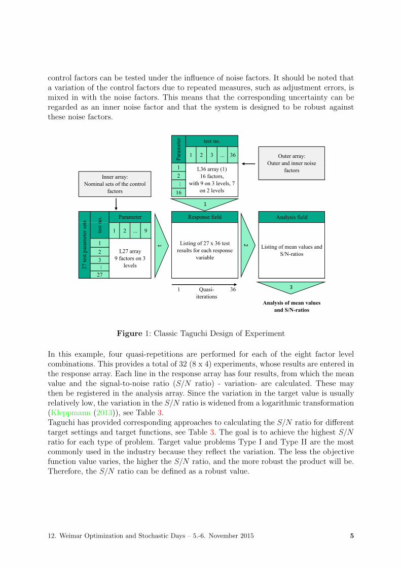
control factors can be tested under the influence of noise factors. It should be noted thata variation of the control factors due to repeated measures, such as adjustment errors, ismixed in with the noise factors. This means that the corresponding uncertainty can beregarded as an inner noise factor and that the system is designed to be robust againstthese noise factors.

1 2 3 ... 36

1

2...

16

Analysis field

1 2 ... 9

1

2

3

...

27

1 36

Analysis of mean values

and S/N-ratios

Listing of mean values and

S/N-ratiosL27 array

9 factors on 3

levels

Par

amet

er

Listing of 27 x 36 test

results for each response

variable

test no.

Outer array:

Outer and inner noise

factors

Inner array:

Nominal sets of the control

factors

Quasi-

iterations

Parameter

27

tes

t par

amet

er s

ets

L36 array (1)

16 factors,

with 9 on 3 levels, 7

on 2 levels

test

no

. Response field

1

2

1

3

Figure 1: Classic Taguchi Design of Experiment

In this example, four quasi-repetitions are performed for each of the eight factor levelcombinations. This provides a total of 32 (8 x 4) experiments, whose results are entered inthe response array. Each line in the response array has four results, from which the meanvalue and the signal-to-noise ratio (S/N ratio) - variation- are calculated. These maythen be registered in the analysis array. Since the variation in the target value is usuallyrelatively low, the variation in the S/N ratio is widened from a logarithmic transformation(Kleppmann (2013)), see Table 3.Taguchi has provided corresponding approaches to calculating the S/N ratio for differenttarget settings and target functions, see Table 3. The goal is to achieve the highest S/Nratio for each type of problem. Target value problems Type I and Type II are the mostcommonly used in the industry because they reflect the variation. The less the objectivefunction value varies, the higher the S/N ratio, and the more robust the product will be.Therefore, the S/N ratio can be defined as a robust value.


Table 3: Adjusted S/N ratio following Taguchi, G. et al. (2005)

Problem type Ideal target function value S/N ratio

Minimization Problem 0 −10 log10

(1n

∑ni=1 y

2i

)Target Value Problem Type I 6= 0, finite 10 log10

(µ2

s2

)Target Value Problem Type II finite −10 log10 (s2)

Maximization Problem ∞ −10 log10

(1n

∑ni=1

1y2i

)yi = target function value; µ = mean value; s = standard deviation

2.2 Robust Design Optimization

In modern development processes, designing for robustness is optimized at an early pro-duct development stage. RDO meets this challenge by using simulation tools. This methodemploys the following steps:

1. Sensitivity analysis,

2. Optimization,

3. Robustness analysis.

2.2.1 Sensitivity analysis

Before a product can be optimized, a profound understanding of both system and productare required, as well as an adequate knowledge of product characteristics. Therefore, themajor factors of product characteristics must be analysed. The results of the analysis allowa determination of which parameters have what effect on the product and its environment,or what correlations they have with each other. This is generally understood as a sensitivityanalysis. The product can be optimized using knowledge from the sensitivity analysis.

2.2.2 Optimization processes

From a mathematical standpoint, optimization is the search for a minimum or maximumfor the target function corresponding to a product characteristic. Various methods andalgorithms have been developed for optimization. The appropriate method should beselected depending on the problem. The most important selection criteria for optimizationare (Gamweger et al. (2009)):

• Number of parameters to be optimized,

• Parameter (continuous, discrete or binary),

• Number of target functions,


• Possible noise of the objective function,

• The need for global optimum-determination.

Optimization methods are, in principle, divided into deterministic and stochastic strate-gies. Examples of the most important methods for are listed in Table 4. Deterministicstrategies are mathematically and technically easier to use and control. A deterministicoptimization method is normally best for an optimization problem with up to 20 para-meters in combination with a single objective function problem.. Tasks with more than100 parameters are processed best using stochastic methods. If several objective functionsare to be considered at the same time, a stochastic process must be used Gamweger et al.(2009). The deterministic ARSM method is applied for the application example presentedin this paper, and is briefly described below.

Table 4: Deterministic and stochastic optimization processes (Kleppmann (2013))

Deterministic Stochastic

Gradient Process, Genetical Algorithms,Direction Search Process, Evolutionary Algorithms,Compass-Search-Process, Pareto-Optimization.Adaptive Response Surface Method.

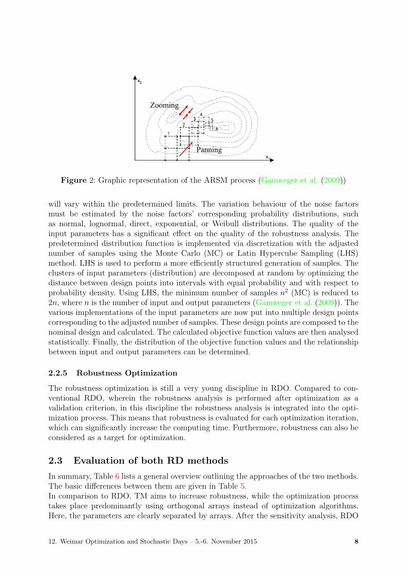
2.2.3 Adaptive Response Surface Method (ARSM)

The ARSM is a highly flexible deterministic optimization method. The principle of thismethod is to locally reproduce the objective function, generally by a linear or quadraticapproximation. The local optimum can be determined very quickly on this analyticallydescribed approximation surface (Kleppmann (2013)). First, the mesh points are calcu-lated for the approximation in a sub-region of the parameter space. The number andlocation of mesh points depends on the order of the approximation and the number ofparameters. This procedure corresponds to the statistical design of experiments (DOE)in the classic product development process. Next, the approximation is spanned at themesh points and the local optimum is determined. This serves as the new centre pointfor the next approximation surface, see Figure 2. Here, the approximation surface will bemoved (panning) and / or resized (zooming). This step is repeated until the difference ofthe results is below the predetermined convergence criterion in two consecutive iterationsteps. This optimum is determined for the approximation. Therefore, the actual optimumhas to be recalculated with the same parameter combination using the original objectivefunction. The approximation quality depends on the difference between the approximatedand actual function values (Gamweger et al. (2009)).

2.2.4 Robustness analysis

After the optimal performance parameter setting has been found, the effect of inevitablyvarying noise factors must be determined. The goal is that desired product characteristics


Panning

Zooming

Figure 2: Graphic representation of the ARSM process (Gamweger et al. (2009))

will vary within the predetermined limits. The variation behaviour of the noise factorsmust be estimated by the noise factors’ corresponding probability distributions, suchas normal, lognormal, direct, exponential, or Weibull distributions. The quality of theinput parameters has a significant effect on the quality of the robustness analysis. Thepredetermined distribution function is implemented via discretization with the adjustednumber of samples using the Monte Carlo (MC) or Latin Hypercube Sampling (LHS)method. LHS is used to perform a more efficiently structured generation of samples. Theclusters of input parameters (distribution) are decomposed at random by optimizing thedistance between design points into intervals with equal probability and with respect toprobability density. Using LHS, the minimum number of samples n2 (MC) is reduced to2n, where n is the number of input and output parameters (Gamweger et al. (2009)). Thevarious implementations of the input parameters are now put into multiple design pointscorresponding to the adjusted number of samples. These design points are composed to thenominal design and calculated. The calculated objective function values are then analysedstatistically. Finally, the distribution of the objective function values and the relationshipbetween input and output parameters can be determined.

2.2.5 Robustness Optimization

The robustness optimization is still a very young discipline in RDO. Compared to con-ventional RDO, wherein the robustness analysis is performed after optimization as avalidation criterion, in this discipline the robustness analysis is integrated into the opti-mization process. This means that robustness is evaluated for each optimization iteration,which can significantly increase the computing time. Furthermore, robustness can also beconsidered as a target for optimization.

2.3 Evaluation of both RD methods

In summary, Table 6 lists a general overview outlining the approaches of the two methods.The basic differences between them are given in Table 5.In comparison to RDO, TM aims to increase robustness, while the optimization processtakes place predominantly using orthogonal arrays instead of optimization algorithms.Here, the parameters are clearly separated by arrays. After the sensitivity analysis, RDO


considers all or only the significant control and noise factors depending on simulationstrategy and capacity. The significant parameters, which may be both noise and controlfactors, are preferred. This is because too many parameters can affect the approximationquality of the Meta model and the optimization algorithm, and more noise can occur. InTM, it is easier to take into account all parameters by using a larger orthogonal array forthe DOE. However, in this case the tolerance limits must be chosen wisely by Meng et al.(2010), since their significance would otherwise be ignored.

Table 5: The procedure of RDO and TM in comparision

1. System and parameter examination2. Design of the simulation model (in TM not necessary)3. Implementation of the sensitivity analysis and determination of the MOP

RDO TM

4. Determination of the distribution 4. Determination of the parameter testfunction levels

5. Selection of the optimization process 5. DOE (orthogonal arrays)6. Optimization with the target value

and the constraints6. Reduction of the variation

7. Adaption of the mean value

Table 6: Fundamental differences of RDO and TM

RDO TM

- only sensitive design parameters are - obvious separation of the parameterconsiderd through arrays

- target value and constraints are preset - no direct preset of constraints- simultaneous optimization of µ and σ - separated optimization of µ and σ- optimum not usually technically - parameter dimensioning on

feasible production engineering points of view

Both methods have the common goal of defining a robust design. However, the two me-thods use different approaches and optimization procedures to achieve this goal, see Table5. The effects of the design parameters are examined through various implementation me-thods (sampling or DOE) of the distribution function. TM is mainly limited to identifyingthe main effects, while RDO can also consider correlations. In RDO, the optimization isrealised using different algorithms, and in TM by reducing variation with subsequent ave-rage adjustment. The adjustment levels of the parameters must be set using TM for thispurpose. In this regard, and due to complex simulations or real experiments, the use ofTM is recommended.


3 Service Brake

Today in Europe, commercial vehicles are almost always equipped with pneumaticallyoperated disc brakes (Breuer and Bill (2012)). The common form uses a structure with afloating brake calliper, which provides a double-sided braking force effect with unilateraloperation. The pneumatic disc brake described here is designed with two punches totension and with a floating calliper.

3.1 Function

When the driver actuates the service brake, the lever (1), Figure 3, is operated by theconnecting rod of the pneumatic cylinder (not shown in the figure) and the rotationalmovement of the lever by means of an eccentric bearing. Thus, a translational displa-cement of the traverse is achieved. The traverse, also referred to as a bridge, includesthe absorption of the threaded spindle and the synchronization unit between them. Thetransmission is constant due to the construction of the lever, amplifying the braking for-ce. Plungers secured to the threaded spindles transfer the translational movement of theinner brake pad (2). When the brake is actuated, the distance between the inner brakepad and the brake disc (3), called the clearance, has to be overcome, so that when thetwo components come into contact, the braking force can be initiated to decelerate thevehicle. The floating calliper inside the brake carrier (4) also initiates the braking forcethrough the outer coating.

12. Weimarer Optimierungs- und Stochastiktage – 05.-06. November 2015 10

3.1 Funktionsweise

Bei Betätigung der Betriebsbremse durch den Fahrzeugführer wird der Hebel (1), Abbildung

3.1, durch das Pleuel des Pneumatikzylinders (im Bild nicht dargestellt) betätigt und aus der

Rotationsbewegung des Hebels mittels exzentrischer Lagerung, eine translatorische

Verschiebung der Traverse erreicht. Die Traverse, auch als Brücke bezeichnet, beinhaltet die

Aufnahme der Gewindespindel sowie die Synchronisierungseinheit zwischen diesen. Durch

die konstruktiven Begebenheiten des Hebels wird eine konstante Hebelübersetzung

bewerkstelligt, welche die Bremskraft verstärkt. Durch Druckstücke, die an den

Gewindespindeln befestigt sind, wird die translatorische Bewegung an den inneren

Bremsbelag (2) übertragen. Beim Betätigen der Bremse muss der Abstand des inneren

Bremsbelags zur Bremsscheibe (3), das sog. Lüftspiel, überwunden werden, damit bei

Kontakt der beiden Komponenten die Bremskraft zur Verzögerung des Fahrzeugs eingeleitet

werden kann. Durch den im Bremsträger (4) schwimmend gelagerten Bremssattel erfolgt eine

Einleitung der Bremskraft ebenfalls durch den äußeren Belag.

Abbildung 3.1: Air Disc Brake

3.2 Nachstelleinheit

Um den Verschleiß der Bremsbeläge sowie der Bremsscheibe während des Betriebs

auszugleichen, wird ein Verschleißnachstellsystem (5) verbaut. Die Wirkungsweise dieses

mechanischen Systems ist unabhängig verschiedener Bauarten identisch [17]. Die Betätigung

der Nachstelleinheit erfolgt durch Betätigung der Betriebsbremse. Das im Leerhub der

Bremse zu überwindende Lüftspiel wird durch geometrische Begebenheiten der Bremse

bestimmt und durch die konstruktive Auslegung des Nachstellers eingestellt.

Abbildung 3.2: Adjusting Unit

1 2 3 4 5

5.1 5.2

Figure 3: Air Disc Brake

3.2 Adjusting Unit

An wear adjustment system (5) is installed to compensate for the wear on the brake padsand the brake disc during operation. The operation of this mechanical system is identicalregardless of brake type (Breuer and Bill (2012)). The actuation of the adjusting unit is


affected by actuation of the service brake. The clearance to be overcome in the idle strokeof the brake clearance is determined by the geometric parameters of the brake and set bythe structural design of the adjuster.

12. Weimarer Optimierungs- und Stochastiktage – 05.-06. November 2015 10

3.1 Funktionsweise

Bei Betätigung der Betriebsbremse durch den Fahrzeugführer wird der Hebel (1), Abbildung

3.1, durch das Pleuel des Pneumatikzylinders (im Bild nicht dargestellt) betätigt und aus der

Rotationsbewegung des Hebels mittels exzentrischer Lagerung, eine translatorische

Verschiebung der Traverse erreicht. Die Traverse, auch als Brücke bezeichnet, beinhaltet die

Aufnahme der Gewindespindel sowie die Synchronisierungseinheit zwischen diesen. Durch

die konstruktiven Begebenheiten des Hebels wird eine konstante Hebelübersetzung

bewerkstelligt, welche die Bremskraft verstärkt. Durch Druckstücke, die an den

Gewindespindeln befestigt sind, wird die translatorische Bewegung an den inneren

Bremsbelag (2) übertragen. Beim Betätigen der Bremse muss der Abstand des inneren

Bremsbelags zur Bremsscheibe (3), das sog. Lüftspiel, überwunden werden, damit bei

Kontakt der beiden Komponenten die Bremskraft zur Verzögerung des Fahrzeugs eingeleitet

werden kann. Durch den im Bremsträger (4) schwimmend gelagerten Bremssattel erfolgt eine

Einleitung der Bremskraft ebenfalls durch den äußeren Belag.

Abbildung 3.1: Air Disc Brake

3.2 Nachstelleinheit

Um den Verschleiß der Bremsbeläge sowie der Bremsscheibe während des Betriebs

auszugleichen, wird ein Verschleißnachstellsystem (5) verbaut. Die Wirkungsweise dieses

mechanischen Systems ist unabhängig verschiedener Bauarten identisch [17]. Die Betätigung

der Nachstelleinheit erfolgt durch Betätigung der Betriebsbremse. Das im Leerhub der

Bremse zu überwindende Lüftspiel wird durch geometrische Begebenheiten der Bremse

bestimmt und durch die konstruktive Auslegung des Nachstellers eingestellt.

Abbildung 3.2: Adjusting Unit

1 2 3 4 5

5.1 5.2

Figure 4: Adjusting Unit

When the service brake is actuated, the rotational movement of the lever is transferredto the adjuster via a gear (5.1), activating the adjustment process. The constructiveclearance must first be overcome. Then the actual adjustment process starts. For anexisting operating clearance that deviates from the adjusted constructive clearance, theclearance is gradually reduced at any level of brake application until the deviation hasbeen compensated for. The particular adjusting operation at the initiation of braking isperformed until the fit between the pads and the brake disc leads to a disproportionatelygreat increase in force, activating the overload protection of the adjusting unit. Whenthis occurs, the adjuster is decoupled from the power flow and the adjustment processis completed. The introduced rotational movement during the resetting of the brake isdecoupled using a free wheel, where a compliance of the set clearance is ensured.Constant clearance set using various functional parameters. After the examination ofKemmler et al. (2014), see chapter 4, the intrinsic free plays of the adjusting unit havebeen identified as highly significant parameters in terms of objective function, a constantand nominal clearance. The internal system free plays of the adjuster unit are describedbriefly below.

3.3 Constructive clearance

The constructive clearance describes the structural clearance which adjusts itself duringoperation. It is determined by the interlocking of the lever wheel and the adjust gear wheelwhich significantly influences the operational clearance of the disc brake.

3.4 Output clearance

The output clearance is formed between the shaft drive (5.2) and threaded pipe (notshown). The rotational motion is transferred to the threaded pipe through the form-fittingconnection, and the clearance is adjusted when abrasion occurs through the translatio-nal movement of the spindle. Depending on the size of the clearance of the form-fittingconnection, it is possible to adjust the clearance with respective accuracy to the structu-rally defined value.


4 Application of SIM-SMAR2T and display of the

results

The assembly adjusting unit was modelled and analysed according to the simulation strat-egy presented in Kemmler et al. (2014) for system analysis using parametric studies afterTM. Meta models (MOP) of the operating torques of the respective operation modeshave been created for this purpose. A Taguchi experimental design was constructed inoptiSLang to keep the software interface interference as low as possible during the virtualexperiments for reasons of time and cost efficiency. Combining different optiSLang moduleblocks and the internal MOP solver facilitates the creation of an efficient approach withregards to time for experimental designs with more than 30 parameters to be examined.An overview of the model is shown in Figure 5. Here, the system of the adjusting unit ismodelled with MOPs of the individual operating modes (Kemmler et al. (2014)).The output graphs of the monitoring modules in Figure 5 show the two operating torquesof the operation modes adjustment and overload protection using the currently evaluatedparameter settings.Figure 6 shows the overall model of a Taguchi experimental design, which includes theoverall model of the adjusting unit (Figure 5), extended using additional optiSLang ele-ments. This addition allows the generation of Taguchi experimental designs with a com-bination of the respective parameters of inner and outer arrays. Creating a Taguchi expe-rimental design in optiSLang will be described in the next section.

Figure 5: Total model adjuster unit


4.1 Creating a Taguchi Design of Experiment in optiSLang

To perform a variety of virtual experiments in a cost-effective manner, it is beneficial tokeep software interface interference low, since running programs in batch mode can lead toincreased time exposure. According to the simulation strategy described in Kemmler et al.(2014), the use of an outer MOP Solver by the company DYNARDO GmbH, which can beaccessed and controlled from the MATLAB environment is assumed. Integrating MOPswith high level of detail causes the software interface to take a considerable amount oftime to pass through automated loop functions. A procedure was developed to minimizethe software interface and the resulting time.The model of Taguchi experimental presented in this paper was designed consideringthe aforementioned goals of creating a time-effective simulation with a small number ofsoftware interfaces. A special feature of the model described is the fact that instead ofindividual discrete response values, a torque curve containing a defined angle size is theoutput. The schematic structure is explained in detail below with reference to Figure 6.Different optiSLang elements must be connected to one another in a work-around toconstruct a Taguchi experimental design in optiSLang. The feature of the proposed model isthe parameter definition in the main level and a targeted remittance of global and intrinsicparameters to the respective MOPs, which are modeled in sub-levels. The addressed mainlevel is a sensitivity-environment (“Taguchi Testing“). All examined system parametersare declared in this main level. Care must be taken to maintain consistent parameter namesin the main and sub-levels. The outer array of the noise factors, see chapter 2, is inputin the main level as StartDesigns for the sensitivity environment, using bin-file import.DYNARDO provides an Excel Add-on to create the bin files from a CSV spreadsheet. Thenoise factors are already registered in this three-stage classification. Dummy values arestored in the StartDesign for the control factors, which will be replaced automatically whenthe workflow is executed with the respective values. The parameters of the outer arrayare classified as parameter type “Optimization“, the internal parameters are classified asthe parameter type “Stochastic“.The actual StartDesigns are created through an automated, script-controlled combinati-on of inner and outer parameters with a Python2 integration module, then transferredto a robustness environment (SIM SMAR2T). The inner parameters are connected as acsv-import with a Path Element to the input channel of the Python2 module for thispurpose. The StartDesigns of the main level are linked to the respective angle values ofthe angle curve through the Python2 module within the robustness environment, therebycreating a number of sub-designs for each main design. The number of angle values tobe examined depends on the level of detail, and can be adjusted. Each sub-design inclu-des the parameters from the main level extended by the variable parameter angle. Thesesub-designs are then sent to the respective MOPs and evaluated. A torque curve over thedefined angle of rotation is the response size as a result obtained with this procedure foreach main design.Using downstream data mining, modules are applied to export and cache the torque cur-ve of the current design by outsourcing in an Excel spreadsheet. Afterwards the torquecurves are re-imported and sent as an input to a Matlab module.Caching is necessary to prevent a mixing of the response curves for the individual runs


Figure 6: Taguchi Design of Experiment in optiSLang

ComponentsK ballCW cone washerLB bearing bushingLS bearing washerPS adjusting washer

AbbreviationAS output clearanceD_I Inner diameterphi angleEZ short lever arm (X)KS constructive clearanceZFS flank clearancey_EZ short lever arm (Y)z_H distance lever-brake

phi_AS (41 %)

E-Modulus_LS_LB (<1 %)

E-Modulus_CW (<1 %)

E-Modulus_K (<1 %)

D_I_PS (<1 %)

D_I_LB (<1 %)

Z_H (1 %)

phi_ZFS (9 %)

y_EZ (12 %)

phi_KS (36 %)

Inpu

t Par

amet

er

10

8

6

4

2

0 20 40 60 80

Coefficient of Importance (CoI) [%]

Figure 7: Results of the simulation after SIM-SMAR2T


within the main designs. Target values for the current main designs are determined withthe generated torque curve using an M-script code implemented in the Matlab module,then sent to the main level (“Taguchi testing“). The software interface to Matlab is ne-cessary due to the use of symbolic variables.Through a detailed sensitivity analysis of the simulation results, the intrinsic clearan-ces of the adjusting unit were determined as highly significant in the objective function“constant clearance“, see Figure 7.An optimization of the parameter output clearance will follow in the next section based onthese results. Optimization using RDO is applied, and a parameter optimization accordingto the procedure of TM is performed.

5 Parameter optimization after RDO and TM in

optiSLang

This chapter describes parameter optimization according to RDO and to the TM basedon the example of output clearance (AS). Finally, the optimization results from bothmethods are compared and discussed.

5.1 Parameter optimization after RDO

After the definition of the parameter space and the limits of variation, the sensitivityanalysis conducted in the next step. For an optimal and sufficient approximation qualityof the MOP, it is advisable to simulate 100 design points in the parameter space. However,this procedure can require a large amount of effort, depending on the simulation model.For this purpose, the developer should apply an appropriate simulation strategy in ad-vance in order to achieve a good compromise between cost, resources and target accuracyKemmler et al. (2014).

5.1.1 Sensitivity analysis

The sensitivity analysis in optiSLang is used to create the MOP, whose quality has adecisive influence on the optimization result. After the sensitivity analysis is performed,the significances of all parameters and their possible correlations can be identified. Thenon-significant parameters can be neglected for increased optimization efficiency in thesubsequent process.The results of the sensitivity analysis and the MOP with a quadratic regression withoutcoupling terms is shown in Figure 8. Accordingly, the depth and the radius of the in-terlocking of the sleeve (D H VZ I, R H VZ) are most significant for the AS. However,they have large variation limits, which can easily enhance their significances. According toMost and Will (2011), the approximation quality of the Meta model is reduced when thenumber of parameters increases. The number of parameters also affects the optimizationmethod in the subsequent process. For this reason, only the 8 most significant parametersare considered when creating the Meta model.


47 %INPUT: D_H_VZ_I

40 %INPUT: R_H_VZ

18 %INPUT: R_SpH_VZ

3 %INPUT: D_SpH_VZ_A

3 %INPUT: R_SpH_R_A

0 %INPUT: W_H_A

0 %INPUT: X_rot_SpH_0

0 %INPUT: Y_rot_SpH_0

Coefficients of Prognosis (using MoP)full model: CoP = 98 %

806040200CoP [%] of OUTPUT: W_AS

86

42

INP

UT

par

amet

er

4.0

3.5

3.0

2.5

2.0

1.5

1.0

0.5

0W

_AS

Polynomial regression of W_ASCoefficient of Prognosis = 98 %

0.550.65

0.750.85

0.951.05 30.1

30.029.9

29.829.729.6

29.5

D_H_VZ_IR_H_VZ

Figure 8: Significance of the parameter of the output clearance (left) and the MOP withquadratic regression with non-coupled terms (right)

5.1.2 Identification of interactions

According to Most and Will (2011) correlations are particularly important when the sumof the individual Coefficient of Prognosis (CoP) values of parameters is larger than thetotal CoP of the Meta model; that means:∑

CoP (Xi) > CoPMeta . (1)

For the AS, the results are∑CoP (Xi) = 111 %, and the CoPMeta = 98 %; accordingly,

there are small correlations. However, the sensitivity analysis detects the parameters bet-ween which correlations exist. Contradicting the MOP has no coupling terms for the AS,which mathematically indicates that no correlations exist between the parameters in theMOP. To explain the contradiction, another examination of parameters has to be carriedout using the significant parameters. A new variable A VZ is defined as follows to explainthe correlation:

A V Z =D H V Z I −D SpH V Z A

2. (2)

A_VZ

Figure 9: Radial distance of the interlock (left) an the contact surface with differentradial distances (middle and right)


A VZ here corresponds to the radial distance of the interlock. A correlation between theaxial distance A VZ and the tangential distance of the interlock exists, which is in turndependent on the parameters R H VZ and R SpH VZ. Figure 9 shows the effect of gra-dually decreasing A VZ, which means that the contact surface shifts downwards to theflank centre. In this case, the change in the radius of the interlock would have the contraryeffect on the clearance.In conclusion, the correlation in the Meta model can be neglected based on these facts.One reason for this is that the correlation exists only in a very small sub-region of theparameter space. In this case, it is probably necessary to create a Meta model with hig-her model accuracy for the entire parameter space, if the correlation is not considered.Another possible reason for this is that the correlation cannot be modeled with a simplemathematical model. Furthermore A VZ is an indirect input parameter, which can leadto the correlation being neglected. In addition, the correlation is covered by main effectsin such a high dimensional problem.

5.1.3 Handling with interactions

The robustness analysis is only recognized if a correlation exists. Further studies are nee-ded to identify the correlation exactly. The mathematical function of the MOP can onlybe displayed in optiSLang if the Meta model has been created using a linear or quadraticregression. These correlations are detected by coupling terms of corresponding parameters.The monomial x1 x2 for example, points to the correlation between the parameters x1 andx2. The functions can not be displayed with other regression methods, due to the highlevel of complexity. If the correlations on the mathematical function can not be preciselyidentified, the system and / or the result before the optimization has to be analyzed moredeeply, especially the apparently erroneous results.To increase the approximation quality of the Meta model, the correlation can be ignoredif the designs can not be applied in this sub-region, in which the detected correlation canoccur. Using the example of AS, this subsection is excluded from the entire parameterspace. In many cases, this method can be applied in industrial settings, because a corre-lation is selectively removed for the majority of products.If a good prediction in the sub region under the influence of correlations is required forother products, other measures have to be applied. Possible measures include:

• Local Meta models are created separately for the sub regions under the influence ofthe correlation. Then these Meta models are integrated into the global MOP.

• Several local Meta models are integrated into an overall MOP (nested) in the entireparameter space. This reduces difficulty by creating a local model, but the selectionof the box areas must be carefully considered. This method can be compared withthe MLS, however, it is more elaborate and may reflect a very complex reality.

Therefore, in applying both methods we must consider that, on the one hand, the integra-tion must be easy to implement and automate and that, on the other hand, the potentialinaccuracies must be corrected in the limit or overlapping areas of the boxes with a specialmethod.


5.1.4 Defintion of the target

In this application example the required objective function value of the AS is:

ΦAS = 0.7◦ ± 0.2◦ . (3)

The AS refers to the middle of the flanks. In a high-dimensional problem, it could bean infinite number of solutions without further restrictions (other objective functions orconstraints). Therefore, in comparison to classic product optimization - i.e., sequentialoptimization procedures with subsequent robustness evaluation - the robustness is inte-grated here as a second optimization target into the optimization process by performinga robust optimization. The variation of the AS should be as small as possible in orderto develop an appropriately robust product. Therefore the clearance ΦAS and variation σacting as a robustness coefficient are defined as objective functions.

5.1.5 Robustness Optimization

In this case, the robustness coefficient will be kept as small as possible, as will the va-riation. There are also other common definitions for the robustness coefficient, such asthe S/N ratio (signal-noise factors ratio) in TM, which correlates well with the standarddeviation σ. The various robustness coefficients can be easily converted to one another.According to the results of the sensitivity analysis, the geometry parameters have a deci-sive influence on the AS. In reality, the manufacturing tolerances of the geometry parame-ters must be considered as noise factors. All tolerances must be translated into actuallyoccurring variations. The geometry parameters are described by these, i.e., by normaldistributions. In this application example, the manufacturing processes have a processcapability index CpK of 1.33, which corresponds with state of the art technology. Thetolerance of the geometric parameters of the standard deviation σ can be converted usingthis information, in this case by dividing by four. The process capability index CpK isdescribed by the mean value µ, the standard deviation σ, and the upper (USL) or lower(LSL) specification limit as follows (Roenpage and Lunau (2007)):

CpK =min(µ− USL;LSL− µ)

3σ. (4)

Table 7 gives an overview of all geometry parameters with their tolerances and standarddeviations σ. In this application example, the coefficient of variation CV is the ratio ofstandard deviation σ and mean value µ (Dynardo (2010)):

CV =σ

µ· 100 % . (5)

A normal distribution is uniquely defined with the specific mean value µ and standarddeviation σ. Then the distributions are realized over a discretization by ALHS and therobust optimization performed by ARSM. The multi objective function problem can besimplified into a single objective function problem with the set target of ΦAS = 0.7◦±0.2◦,because the target size of AS is defined as a boundary condition within the optimization.Accordingly, the robustness value σ is the only objective function. It should be consideredthat the constraint at optiSLang can only be defined in terms of comparison signs.


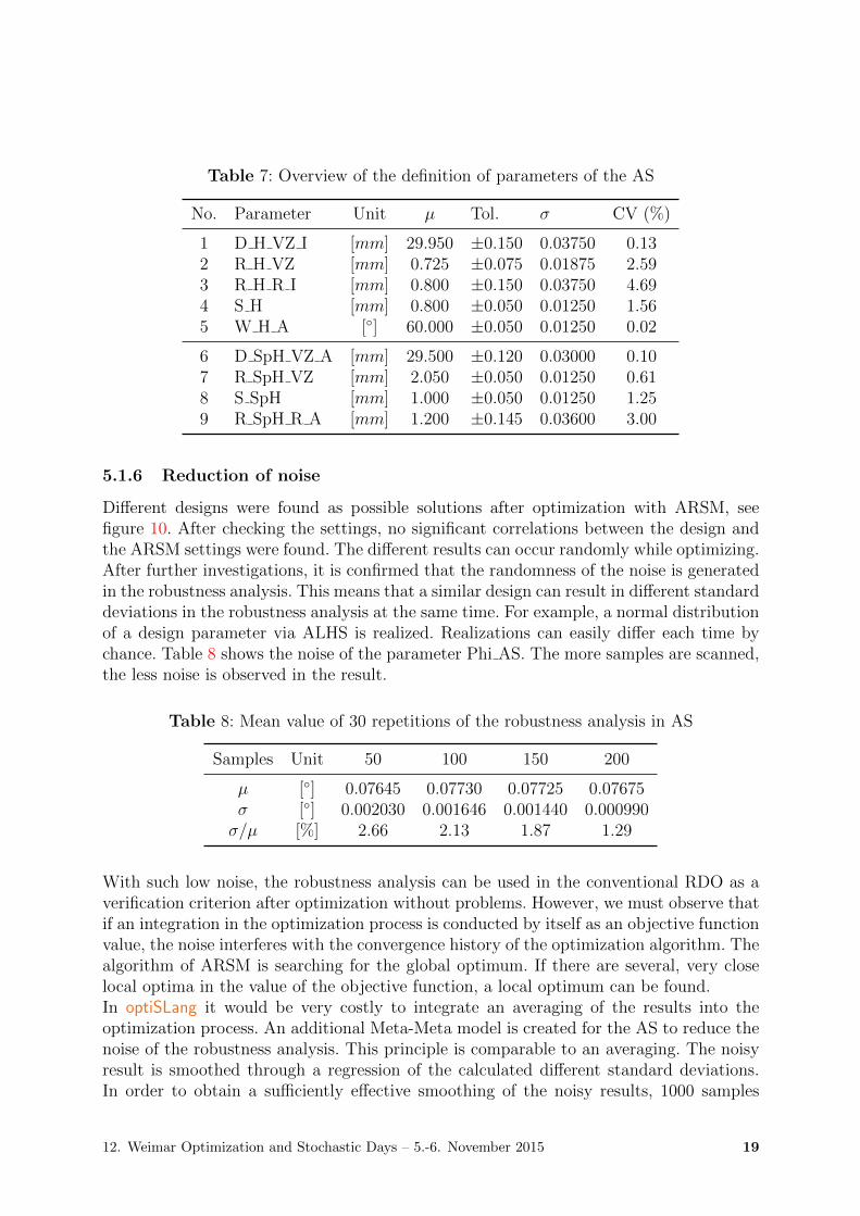
Table 7: Overview of the definition of parameters of the AS

No. Parameter Unit µ Tol. σ CV (%)

1 D H VZ I [mm] 29.950 ±0.150 0.03750 0.132 R H VZ [mm] 0.725 ±0.075 0.01875 2.593 R H R I [mm] 0.800 ±0.150 0.03750 4.694 S H [mm] 0.800 ±0.050 0.01250 1.565 W H A [◦] 60.000 ±0.050 0.01250 0.02

6 D SpH VZ A [mm] 29.500 ±0.120 0.03000 0.107 R SpH VZ [mm] 2.050 ±0.050 0.01250 0.618 S SpH [mm] 1.000 ±0.050 0.01250 1.259 R SpH R A [mm] 1.200 ±0.145 0.03600 3.00

5.1.6 Reduction of noise

Different designs were found as possible solutions after optimization with ARSM, seefigure 10. After checking the settings, no significant correlations between the design andthe ARSM settings were found. The different results can occur randomly while optimizing.After further investigations, it is confirmed that the randomness of the noise is generatedin the robustness analysis. This means that a similar design can result in different standarddeviations in the robustness analysis at the same time. For example, a normal distributionof a design parameter via ALHS is realized. Realizations can easily differ each time bychance. Table 8 shows the noise of the parameter Phi AS. The more samples are scanned,the less noise is observed in the result.

Table 8: Mean value of 30 repetitions of the robustness analysis in AS

Samples Unit 50 100 150 200

µ [◦] 0.07645 0.07730 0.07725 0.07675σ [◦] 0.002030 0.001646 0.001440 0.000990σ/µ [%] 2.66 2.13 1.87 1.29

With such low noise, the robustness analysis can be used in the conventional RDO as averification criterion after optimization without problems. However, we must observe thatif an integration in the optimization process is conducted by itself as an objective functionvalue, the noise interferes with the convergence history of the optimization algorithm. Thealgorithm of ARSM is searching for the global optimum. If there are several, very closelocal optima in the value of the objective function, a local optimum can be found.In optiSLang it would be very costly to integrate an averaging of the results into theoptimization process. An additional Meta-Meta model is created for the AS to reduce thenoise of the robustness analysis. This principle is comparable to an averaging. The noisyresult is smoothed through a regression of the calculated different standard deviations.In order to obtain a sufficiently effective smoothing of the noisy results, 1000 samples


Phi_AS_vali = 0.434° Phi_AS_vali = 0.451°

Phi_AS_vali = 0.468° Phi_AS_vali = 0.455°

Design Number # 240 Design Number # 180

Design Number # 216Design Number # 276

Relative Size of Bounds [%] Relative Size of Bounds [%]

Relative Size of Bounds [%]Relative Size of Bounds [%]

Par

amet

ers

Par

amet

ers

Par

amet

ers

Par

amet

ers

R_SpH_VZ1.765

R_SpH_R_A1.0063

R_H_VZ0.90882

D_SpH_VZ_A29.359

D_H_VZ_I29.634

R_SpH_VZ1.7633

R_SpH_VZ1.7377

R_SpH_VZ1.7068

R_SpH_R_A1.0235

R_SpH_R_A1.2548

R_SpH_R_A0.87933

R_H_VZ0.8763

R_H_VZ0.76319

R_H_VZ0.86282

D_SpH_VZ_A29.438

D_SpH_VZ_A29.381

D_SpH_VZ_A29.458

D_H_VZ_I29.677

D_H_VZ_I29.59

D_H_VZ_I29.661

Figure 10: Optimized designs with different ARSM settings, Meta model with 8 parame-ters, W H A = 60◦, set value 0.45 %

16 %INPUT: R_SpH_VZ


2 %INPUT: D_H_VZ_I

2 %INPUT: R_H_VZ

0 %INPUT: R_SpH_R_A

0 %INPUT: W_H_A


100806040200CoP [%] of OUTPUT: Sigma

65

43

21

INP

UT

par

amet

er

0.160

Sigm

a

Polynomial regression of SigmaCoefficient of Prognosis = 23 %

29.35

2.001.95

1.901.851.80

1.75

R_SpH_VZD_SpH_VZ_A

0.156

0.152

0.148

0.144

29.4029.45

29.5029.55

Figure 11: The significance of the parameter (left) and the Meta-Meta model of theoutput clearance (right)


are tested by the ALHS method to construct the Meta-Meta model. According to theCoP -value of 23 %, the approximation quality of the Meta-Meta model is not sufficient.However, a lower CoP is acceptable or even expected, because the CoP is ensued by avariance-based statistical method. The CoP indicates the percentage of the variance ofthe system response covered by the regression. The variance with noise is not completelyaccounted for by regression. Figure 11 directly demonstrates the significance of each designparameter for the robustness (variation). According to it, the parameter R SpH VZ hasthe most impact on the AS.The convergence curve during the optimization process is an important indicator forthe efficiency and accuracy of the results. With consideration of the noise, the objectivefunction value σ converges insufficiently and slowly - up to 30 iterations - to the localoptimum, while without consideration of the noise it converges quickly to the globaloptimum (up to 10 iterations), see Figure 12.

Optimzation Designs Optimzation Designs

Obj

ecti

ve V

alue

s

250 300

Best designs (complete)

150100500 806040200

Objective History of Support Points Objective History of Support Points

100

Objective data for all support Support points

Best designs (complete)Objective data for all support Support points

0.14

0.14

250.

145

0.14

750.

150.

1525

0.15

5

0.14

850.

149

0.15

0.15

10.

152

Figure 12: Comparision

The design determined by the Meta-Meta model is finally validated by 30 repetitive ro-bustness analyses using the Meta model. The mean value of the 30 standard deviationscorresponds very well with the results from the Meta-Meta model. The results from RDOare listed in comparison to the results of TM in Section 5.3.

5.2 Parameter optimization according to TM

The parameter space for the sensitivity analysis and for the Meta model must first bedefined. Compared to RDO, TM after SMAR2T Kemmler et al. (2015) considers boththe significant and the insignificant parameters for the sensitivity analysis and as wellfor creating the Meta model, which means that the full parameter space is examined inAS. The MOP is a quadratic regression without coupling terms involving no correlation,see Figure 13. The CoP of the Meta model of 98 % is quite satisfying, but the sum of


the individual CoP is 120 %. The correlation due to small A VZ must be eliminated,according to RDO.

52 %INPUT: D_H_VZ_I

42 %INPUT: R_H_VZ

20 %INPUT: R_SpH_VZ


3 %INPUT: R_SpH_R_A

0 %INPUT: Mu

0 %INPUT: W_H_A

0 %INPUT: BT


806040200CoP [%] of OUTPUT: W_AS

86

42

INP

UT

par

amet

er

4.0

W_A

S

Polynomial regression of W_ASCoefficient of Prognosis = 98 %

0.60

30.029.9

29.829.729.6

29.5

D_H_VZ_IR_H_VZ

0.700.80

0.901.00

3.5

3.0

2.5

2.0

1.5

1.0

0.5

0

Figure 13: Significance of all parameters (left) and the MOP: quadratic regression withuncoupled terms (right)

5.2.1 Design of Experiment

As mentioned in Chapter 2, with the Taguchi method an experimental design is createdin order to recognize the effects of the parameters on the objective function. A distinctionis made between inner and outer arrays.

Inner array

Table 9 shows an overview of all control factors on three factor levels. The lower (LSL)and upper limits (USL) of the control factors are each limited to 10 % of the entire areainwards to avoid inaccuracy of the Meta model at the border area. That provides thepossible application of a tolerance analysis, see Figure 14. An orthogonal array L27 isused for nine control factors on three levels (27 experimental settings), see Figure 16.

10 % 10 %

LSL mean value USL

Figure 14: Restriction of the limits of variation

Outer array

Normally, in TM the outer array considers only the outer noise factors that are notconnected to the control factors, such as the variation in operating temperature, materialcharacteristics, and load. The classic Taguchi arrays can be used if


Table 9: Control factors (geometric parameter) on three setting levels for the inner array

No. Parameter Unit UG µ OG

1 D H VZ I [mm] 29.5500 29.8200 30.09002 R H VZ [mm] 0.5775 0.8138 1.05003 R H R I [mm] 0.6400 0.8000 0.96004 S H [mm] 0.6400 0.8000 0.96005 W H A [◦] 44.0000 60.0000 76.000

6 D SpH VZ A [mm] 29.3300 29.4500 29.75007 R SpH VZ [mm] 1.7350 1.8750 2.01508 S SpH [mm] 0.8400 1.0000 1.16009 R SpH R A [mm] 0.8000 1.1000 1.4000

• the control factors do not vary in practice,

• the variation of control factors can not be controlled or is very difficult to estimate,

• there is a linear correlation (first order) between the control factors and the targetvalue.

In other cases, depending on the optimization strategy and capacity, only the significantor even all control factors are considered as noise factors in the outer array.As is apparent from the sensitivity analysis, the control factors (geometric parameters)and their variation from manufacturing tolerances have a decisive influence on the AS. Inaddition, the Meta model is determined from a quadratic regression. In this regard, thesevariations must be considered as internal noise factors.One fundamental difference between TM and RDO is described by the distribution ofthe variation. In RDO, the normal distributions of the input parameters are displayed onsamples, causing the objective function value to be distributed in a realistic manner. Incontrast, the normal distributions of the parameters in TM are converted to an appro-ximately equal distribution (D’Errico and Zaino (1988)). Therefore, the parameters areeither tested on three stages, the upper specification limit (USL), the mean value µ, andthe lower specification limit (LSL), or in two stages (USL, LSL) in order to representthe variation in the system. The transformation can be carried out with the followingnotation:

µ± σ√

3 . (6)

With two stages to be tested, the mean value is neglected. A very good estimation of thevariation of this transformation is achieved after D’Errico and Zaino (1988).For each setting stage of the parameters, the variation of the inner noise factors is conver-ted on three stages. Figure 15 shows the variation of the parameter R SpH VZ, where thestandard deviation is σ = 0.0125. With the notation 6, USL and LSL are set to ±σ ·

√3

or ±0.022.


Inner array:Nominal settings

of parameter R_SpH_VZ

Outer array:Inner noise parameters

UG

µ

OG

1.735

1.875

2.015

1.713

1.853

1.993

1.735

1.875

2.015

1.757

1.897

2.037

Figure 15: Implementation of the inner noise factors on the example of R SpH VZ

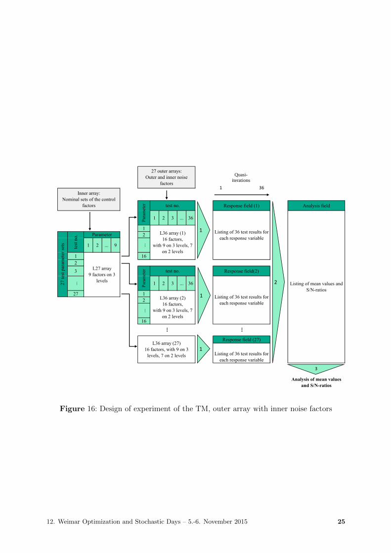
The 9 inner noise factors are tested on three levels, while the 7 outer noise factors aretested on two stages. According to Figure 16, an orthogonal array L36 with 36 tests isneeded for the outer array. A new outer field is created in each test setting of the controlfactors, in which the inner noise factors are adjusted to the nominal values of the controlledfactors. A total of 27 · 36 = 972 tests are performed by the MOP for the subsequent meanvalue and S/N analysis.

5.3 Evaluation of results from the optimization methods

In applying TM, the same Meta model is used as in the RDO, and contains all controland noise factors. After testing 27 · 36 = 972 samples, the effects of the control factors onthe mean value and the S / N ratio of AS are determined see Figure 17. Here, the S/Nratio is calculated by “The nominal best type II“. The higher the S/N ratio, the morerobust the product is.In TM, the variation of the objective function value is initially reduced by setting theadjustment levels for all control factors. This maximizes the S/N ratios. However, withstrict implementation, the mean value shifts. Thus the mean value must be adapted tothe target value. Here, the adjustment levels of the control factors R H VZ, D SpH VZ Aand R SpH VZ are not changed. The subsequent adjustment of the mean value is carriedout by varying the parameters D H VZ I and R SpH R A.Similar trends in the main effects of AS are detected using DOE (TM) and Meta-Metamodel (RDO), especially by the significant parameters D H VZ I, R H VZ, D SpH VZ Aand R SpH VZ, see Figure 17. Table 10 presents a comparison of the best designs fromRDO and TM. For most design parameters, particularly for the significant parameters,there is only a minimal deviation. The deviations cannot be avoided because when apply-ing TM, the control factors are only graded in a very rough manner. The deviations of theparameters S SpH and R SpH R A are relatively large. The reason is that their parameterlevels are set with a small priority for low significances to minimize the deviation of themean value.The robustness analysis by ALHS for the two best designs provides an equal standard de-viation of 0.092◦, when all noise factors are considered. However, the S/N ratios of DOEand ALHS do not correspond correctly. With the application of the Taguchi Method, theoptimized S/N ratio by using DOE is about 18.25 (standard deviation of 0.122◦), compa-red to the S/N ratio of 20.7 using ALHS (standard deviation of 0.092◦). This deviationis caused by the different methods of implementing the distribution function.


Response field (1) Analysis field

1 2 3 ... 36

1

2

1 2 ... 9 ...

1 16

2

3 Response field(2)

... 1 2 3 ... 36

27 1

2

...

16

Response field (27)

Analysis of mean values

and S/N-ratios

Inner array:

Nominal sets of the control

factors

27 t

est

par

amet

er s

ets

test

no. Parameter

L27 array

9 factors on 3

levels

27 outer arrays:

Outer and inner noise

factors

test no.

Par

amet

erP

aram

eter test no.

L36 array (1)

16 factors,


on 2 levels

Listing of 36 test results for

each response variable

L36 array (27)

16 factors, with 9 on 3

levels, 7 on 2 levels

Listing of mean values and

S/N-ratios


each response variable


each response variableL36 array (2)

16 factors,


on 2 levels

1

1

2

3

Quasi-

iterations

1 36

...

1

...

Figure 16: Design of experiment of the TM, outer array with inner noise factors


18.16

D_H_VZ_I

Mea

n o

f SN

rat

ios

R_H_VZ R_H_R_I

W_H_A S_H D_SpH_VZ_A

R_SpH_VZ R_SpH_R_A S_SpH

3029.829.6

D_H_VZ_I

20.65

20.60

20.55

1.00.80.630.129.829.5 1.00.80.5 1.00.80.6 0.90.80.7

R_H_VZ R_H_R_I

75655545

W_H_A

20.65

20.60

20.55

0.90.80.7

S_H

29.629.529.429.3

D_SpH_VZ_A

0.960.800.64 29.629.4529.3766044

1.41.10.8 1.21.00.82.01.851.7 2.01.91.8

R_SpH_VZ

1.31.10.9

R_SpH_R_A

1.21.00.8

20.65

20.60

20.55

S_SpH

18.08

18.00

18.16

18.08

18.00

18.16

18.08

18.00

Figure 17: Results of TM (on the left - Minitab) and RDO (on the right - optiSLang),influence of the noise factors on S/N ratio, with selected setting levelss


Table 10: Comparison of the best designs by RDO and TM

No. Parameter Unit Best Design RDO Best Design TM Deviation [%]

1 D H VZ I [mm] 29.80 29.82 0.072 R H VZ [mm] 0.60 0.58 3.453 R H R I [mm] 0.63 0.64 1.594 S H [mm] 0.77 0.80 3.755 W H A [◦] 54 60 11.11

6 D SpH VZ A [mm] 29.60 29.57 0.107 R SpH VZ [mm] 1.700 1.735 2.358 S SpH [mm] 0.8 1.0 20.009 R SpH R A [mm] 1.1 0.8 37.5.

Phi AS [◦] 0.82 0.79 3.66Sigma all ALHS [◦] 0.091 0.092 (DoE: 0.122) 1.09

*the parameters in bold are significant

*Sigma all: with all noise factors

Table 11: Fundamental differences of RDO and TM

TM RDO

+ relatively simple method + mean value and nominal value areoptimized separately

+ lower number of tests + high automization+ flexible with few parameters + definition of constraints possible

and uncoupled CF and NF+ very robust method, suitable for + fast adaption of the target value

early PDF or validation phase+ Meta modeling not mandatory + fast adaption of new tolerances

(but difficult with noise)+ multiobjective optimization possible+ optimization of up to 100 parameters+ no additional expense when

extending parameters

- manual consideration of constraints - no consideration of non-significant- no definiton of the random parameters

target value


The best design with this present setting level combination is validated by MOP. Thecalculated nominal output clearance is 0.79◦. This imprecision can not be avoided becauseof the coarsely graded control factors. In summary, the two methods provide very similarresults.Compared to RDO, TM considers the four most significant parameters. A smaller outerarray (L9) instead of L36 is used, and a similar design with high accuracy is achieved, whencompared to RDO. In summary, both methods are compared in Table 11 with regards totheir flexibility of application.

6 Instruction RDO and Taguchi

Based on the results presented, we have derived a recommendation for action for applyingthe two methods and visualized it using a flow chart, see Figure 18.

7 Discussion and summary

Many similarities can be found between the two optimization methods, as we have seenin the present investigation. If the same Meta model is used, similar results are achievedusing TM and RDO, and robustness can be optimized. The TM is in general a universallyapplicable method that is mainly used in the statistical design of experiments (DOE).Due to the low number of tests it requires, this method can be used to carry out realexperiments as well as simulations. This means that a Meta model is not mandatory.Possible noise in the results is prevented by converting parameter distribution functionsinto equal distribution with coarsely graded control factors.However, TM is only limited to relatively simple optimization problems with a low numberof parameters due to its manual optimization procedure. If boundary conditions need tobe considered when optimizing, the optimization is more complicated and more expensive.In addition, an optimization aiming towards a coarse gradation of the control factors is notvery easy to achieve. Furthermore, the calculated standard deviation (S/N ratio) shouldonly be used to compare different parameter combinations. The actual value must bevalidated by ALHS because of the inaccurate implementation process of the test variationsor robustness analysis.In comparison with RDO, TM aims primarily to increase system robustness. However,the optimization process is performed manually using orthogonal arrays instead of withthe help of optimization algorithms. The parameters are clearly separated by arrays here,but no multi-objective optimization can be realized.According to the sensitivity analysis, depending on simulation strategy and capacity,either all or only the significant control and disturbance variables are considered. Thesignificant parameters are preferred in RDO, which may be both noise factors and controlfactors. Examination of too many parameters causes noise to affect the approximationquality of the MOP and the optimization algorithm. In TM, it is less expensive to takeall parameters into account by using a larger orthogonal array for the DOE. However,in this case the tolerance limits must be chosen wisely, otherwise the significances arecovered . When optimizing manually, non-significant parameters can be optimized with


Sensitivity analysis

Selection of parameter and

regression function

∑CoP >CoPMeta?

Outer array with NF* and only significant NF

Parameter design

withcoupling terms

(Xi*Zi)?

Polynomialregression

MLS,Kriging

WW existentCF NF

yes

no

Significance of sensitivty

analysisCF significant?

WWnon-existentCF NF Local MOP-

improvement by further designs

RDO

Outer array with NF and only significant

NF*

no

yes

New designspace?yes

noclassic Taguchi-

arrays

Selection of optimization

approach

Adjustment of the optimization

approach

Definition of objective and

boundary conditions

Realization of the distribution

function

σvery noisy

?

Noise reduction by meta-

metamodelyes

Optimization

Legend:Process

Decision

Document/conclusion

Note

CoP Coefficients of Prognosis

MOP Metamodel of Optimal Prognosis

MLS Moving Least Squares

WW ( ) Interaction (between)

CF(Xi) Control factor (control parameter)

NF(Zi) Noise Factor (noise)

NF* Control factor as NF (inner

noise)

F Significant factor

s Standard deviation

MOP

DoE

Taguchi-Analysis

Reduction of variation

Adjustment of mean values

Validation with FE-Modell sufficient? no

Tolerance design

yes

New boundarycondition?yes

Tests (with meta-model)

Taguchi

yes

no

no

MC ALHS

Approach of RDO and simulative Taguchi Method

Gradation of NF*

HighestCoP?

WWexistent

WWnon-existent

yes

no

no

yes

Deter-mination of

the MOP

CF

NF NF*

CF

NF NF*

CF

NF

Determination of the distribution function for NF and NF*,

determination of characteristic values

... ... ...

WW

WWWW

Figure 18: Flow chart pre-processing, RDO and Taguchi - optimization


low priorities at the end.A specific procedure is presented in the form of a flow chart in Chapter 6 as a summaryof this paper, see Figure 18.In further investigations, the integration possibility of the variation should be examinedwith coarse gradation instead of classic sampling in RDO. This would prevent incidentalnoise. Subsequently, optimization with the actual variation of the best designs should bechecked using the robustness analysis with classical sampling. This addition allows theadvantages of both methods to be combined.

Acknowledge

The authors would like to thank Zeyi Wang (B.Sc.) for his intensive cooperation, hisconstructive comments, and his suggestions.

References

Breuer, B. ; Bill, K. H.: Bremshandbuch - Grundlagen, Komponenten, Systeme, Fahrdy-namik. 4. Edition. Berlin : Springer Vieweg Verlag, 2012

D’Errico, J. ; Zaino, N.: Statistical Tolerancing using a Modification of Taguchi’sMethod. American Society for Quality, 1988

Dynardo: OptiSLang - The optimizing structural language. Weimar : dynardo - DynamicSoftware and Engineering GmbH, 2010

Gamweger, J. ; Jobst, O. ; Strohrmann, M.: Design for Six Sigma - Kundenori-entierte Produkte und Prozesse fehlerfrei entwickeln. Munchen : Carl Hanser Verlag,2009

Gundlach, C.: Entwicklung eines ganzheitlichen Vorgehensmodells zur problemorien-tierten Anwendung der statistischen Versuchsplanung. Kassel : Kassel university pressGmbH, 2004

Kemmler, S. ; Bertsche, B.: Gestaltung robuster und zuverlassiger Produkte nach derSMART-Methode. In: Proceedings of the 25th Symposium on Design for X. Bamberg,October 2014, p. 169–180

Kemmler, S. ; Bertsche, B.: Systematic Method for Axiomatic Robustness-Testing(SMART). In: Proceedings of the International Symposium on Robust Design. Copen-hagen, August 2014, p. 101–112

Kemmler, S. ; Dazer, M. ; Leopold, T. ; Bertsche, B.: Method for the development ofa functional adaptive simulation model for designing robust products. In: 11th WeimarOptimization and Stochastic Days. Weimar, November 2014


Kemmler, S. ; Fuchs, A. ; Leopold, T. ; Bertsche, B.: Systematisches ToleranzDesign unter Berucksichtigung von Funktions- und Kostenaspekten nach der robustenZuverlassigkeitsmethode SMAR2T. In: Proceedings of the 26th Symposium on Designfor X. Munchen, October 2015, p. 209–220

Kleppmann, W.: Versuchplanung: Produkte und Prozesse optimieren. Carl Hanser Ver-lag, 2013

Meng, J. ; Zhang, C. ; Wang, B. ; Eckerle, W.: Integrated robust parameter designand tolerance design. In: Int. J. Industrieal and Systems Engineering Vol. 5 (2010),No. No.2, p. 159 – 189

Mori, T.: The New Experimental Design: Taguchi’s Approach to Quality Engineering.Dearborn, MI : ASI Press, 1990

Most, T. ; Will, J.: Sensitivity analysis using the Metamodel of Optimal Prognosis. In:Weimar Optimization and Stochastic Days 2011. Weimar, November 2011

Park, G.-J. ; Lee, T.-H. ; Lee, K. H. ; Hwang, K.-H.: Robust Design: An Overview.AIAA Journal, Vol. 44, p. 181-191, 2006

Roenpage, O. ; Lunau, S.: Six Sigma + Lean Toolset: Verbesserungprojekte erfolgreichdurchfuhren. 2. Edition. Berlin : Springer Vieweg Verlag, 2007

Suh, N. P.: Axiomatic Design - Advances and Applications. New York : Oxford UniversityPress, 2001

Taguchi, G. et al.: Taguchi’s Quality Engineering Handbook. New Jersey : John Wiley& Sons, Inc., 2005


comparison of taguchi method and robust design ... · comparison of taguchi method and robust...

Documents