comparison of robust control techniques … · comparison of robust control techniques for use in...

COMPARISON OF ROBUST CONTROL TECHNIQUES FOR USE IN

ACTIVE SUSPENSION SYSTEMS

Fábio Luis Marques dos Santos, [email protected]

Jorge Augusto de Bonfim Gripp, [email protected]

Alberto Adade Filho, [email protected]

Luiz Carlos Sandoval Góes, [email protected]

Instituto Tecnológico de Aeronáutica

Abstract. In this paper three robust control techniques are addressed - LQG/LTR control, H-infinity mixed sensitivity

control and mu-synthesis control. These were designed to be used in an automotive active suspension system. The

main goal is to obtain robust stability performance, in order to minimize the sprung mass (chassis) acceleration and to

ensure road-holding characteristics. A nonlinear model a hydraulic actuator, in a half-car model, was used to verify the

performance of each control technique. Comparison is then made, by means of numerical simulation, two types of road

profiles.

Keywords: active suspension, robust control, LQG/LTR, mu synthesis, H-infinity

1. INTRODUCTION

The design of robust controllers for use in an active suspension system of a half-car is studied in this paper. The

automotive suspension has a main goal of isolating the passengers inside the car, from road irregularities and other forces

and disturbances such as those from cornering, accelerating and braking. At the same time, the suspension system is also

expected to guarantee good road-handling performance for the vehicle. For long there have been studies on both industry

and academia, to improve the suspension system performance. These studies have led to the active suspension systems.

To better explain these systems, it can be easier to first introduce the so called passive systems.

Passive suspension systems are uncontrolled systems, built with only springs and dampers with unchangeable charac-

teristics. This means that their parameters must be chosen adequately at project level to provide comfort and road handling

while under different road conditions. this leads to a trade-off between road-handling and comfort, where improving one

parameter can lead to the degradation of the other. This is a great motivation on the study of active suspension systems.

The active suspension systems normally use hydraulic actuators (see for example Fischer and Isermann (2004), En-

gelman and Rizzoni (2009), Williams (1997b) and Williams (1997a)), that can act directly on the vertical dynamics of the

suspension, thus improving its performance.

This paper focuses on the design and comparison of robust control techniques applied to the active suspension problem.

This sort of problem has been very well studied in the literature, see Palkovics et al. (2009) and Herrnberger et al. (2008).

Three main robust control techniques are addressed in this work - LQG/LTR control, Mixed-sensitivity H∞ control and

µ-synthesis control (for some practical examples, see Taghirad and Esmailzadeh (1998), Du et al. (2005) and Lauwerys

et al. (2005)). A comparison in then made, by using singular values, structured singular values and temporal impulse

response. Finally, the µ-synthesis technique is simulated using a non-linear actuator, and its performance is compared to

that of a passive suspension system.

2. PROBLEM FORMULATION

The most commonly used models for the suspension control design is the quarter-car and the half-car models (see

D. Karnopp (1974), Hrovat (1993) and all other references). In this paper, the half-car model was used and was taken

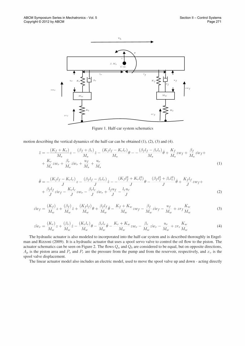
from Canale et al. (2006); Milanese and Novara (2007). The half-car system (Figure 1) consists of an upper sprung

mass Ms, with inertia J , that has two degrees-of-freedom (DOF), the pitch rotation θ and the vertical translation z. The

sprung mass is connected to the front and rear suspension systems, that are modeled as a spring-damper system, with

constant values Kf,r and βf,r - the subscripts f and r shall be used therein to represent the front and rear parts of the

system, respectively. The tires are modeled as a mass-spring system with stiffness Kw and mass Mw, adding another

two DOF’s to the system, zwf and zwr, representing the vertical movement of the tires. All the modeled masses in the

system are considered plainly rigid, for sake of simplicity. The force inputs uf and ur represent the force exerted by

the hydraulic actuators. The inputs zrf and zrr represent the road disturbance due to road irregularities and holes, Vh

represents the vehicle horizontal traveling velocity, which is assumed constant for this model. Also, the parameters lfand lr represent the distance from the center of gravity (C.G.) to the front and rear suspensions, respectively. From

the force equilibrium equations (see also Hrovat (1993); Krtolica and Hrovat (1992) for further details), the equations of

ABCM Symposium Series in Mechatronics - Vol. 5 Copyright © 2012 by ABCM

Section II – Control Systems Page 270

J,Ms

θ

ufur KfKrβr

βf

KtKt

zrrzrf

zwrzwf

z

Vh

C.G.

lr lf

MwMw

Figure 1. Half-car system schematics

motion describing the vertical dynamics of the half-car can be obtained (1), (2), (3) and (4).

z = −(Kf +Kr)

Ms

z −(βf + βr)

Ms

z −(Kf lf −Krlr)

Ms

θ −−(βf lf − βrlr)

Ms

θ +Kf

Ms

zwf +βf

Ms

˙zwf+

+Kr

Ms

zwr +βr

Ms

˙zwr +uf

Ms

+ur

Ms

(1)

θ = −(Kf lf −Krlr)

Jz −

(βf lf − βrlr)

Jz −−

(Kf l2

f +Krl2r)

Jθ −

(βf l2

f + βrl2r)

Jθ +

Kf lfJ

zwf+

+βf lfJ

˙zwf −KrlrJ

zwr −βrlrJ

˙zwr +lfuf

J−

lrur

J(2)

zwf =(Kf )

Mw

z +(βf )

Mw

z +(Kf lf )

Mw

θ +βf lfMw

θ −Kf +Kw

Mw

zwf −βf

Mw

˙zwf −uf

Mw

+ zrfKw

Mw

(3)

zwr =(Kr)

Mw

z +(βr)

Mw

z −(Krlr)

Mw

θ −βrlrMw

θ −Kr +Kw

Mw

zwr −βr

Mw

˙zwr −ur

Mw

+ zrrKw

Mw

(4)

The hydraulic actuator is also modeled to incorporated into the half-car system and is described thoroughly in Engel-

man and Rizzoni (2009). It is a hydraulic actuator that uses a spool servo valve to control the oil flow to the piston. The

actuator schematics can be seen on Figure 2. The flows Qa and Qb are considered to be equal, but on opposite directions,

Ap is the piston area and Ps and Pr are the pressure from the pump and from the reservoir, respectively, and xv is the

spool valve displacement.

The linear actuator model also includes an electric model, used to move the spool valve up and down - acting directly


Section II – Control Systems 71

ApQa

Qb

Ps

Pr

Pr

xv

Figure 2. Hydraulic actuator schematics - piston and spool valve

on xv .

PLf = −4Apβe

Vt

z −Ap4βelf

Vt

θ +Ap4βe

Vt

˙zwf −Kc

Kq4βe

Vt

xvf (5)

xvf = −1

τ2xvf +

τ1τ2

if (6)

PLr = −4Apβe

Vt

z +Ap4βelr

Vt

θ +Ap4βe

Vt

˙zwr −Kc

Kq4βe

Vt

xvr (7)

xvr = −1

τ2xvr +

τ1τ2

ir (8)

Where PLf,r is the load pressure, such that Ap · PL equals to the force exerted by the actuator. The bulk modulus of the

fluid is represented by βe, the total fluid volume is Vt, Kq is the flow gain, Kc is the flow-pressure coefficient and τ1 and

τ2 are the spool valve’s gain and time constant, respectively.

3. CONTROL STRATEGIES

3.1 LQG/LTR Control

The LQG/LTR controller (Kwakernaak (1969), Skogestad and Postlethwaite (1996) ), or Linear Quadratic Gaussian

control with Loop Transfer Recovery, is a control design method that uses a classic LQG controller, and then applies a

procedure to increase its robustness.

The classic LQG control problem consists on finding the optimal control input, u(t), which minimizes (9).

J = E

{

limT→∞

1

T

∫ T

0

[xTQx+ uTRu]dt

}

(9)

where Q and R are the chosen constant weighting matrices. The solution to this problem is achieved by calculating the

optimal controller by solving the Linear Quadratic Regulator Problem, and then designing a Kalman Filter that optimally

estimates the system’s states. Although both LQR and Kalman filter solutions yield good robustness properties to the

controlled system, when used together on the LQG control, they do not guarantee any robustness properties. To recover

the robustness properties inherent to the LQR system, a Loop Transfer Recovery procedure is carried. This procedure,

which is throughly explained in Stein and Athans (1987), uses Q = CTC and R = ρI to obtain the controller, and as ρtends to zero, the LQG loop transfer function tends to that of the LQR controller. On the other hand, as ρ gets smaller, high

controller gains are introduced, which may cause problems with unmodelled dynamics, so the best solution is achieved

on an iterative procedure, so that the gains are kept low.



3.2 Mixed-sensitivity H∞ Control

The Mixed-sensitivity H∞ control design consists of the design of the H∞ optimal controller while shaping the

sensitivity function S, the closed loop transfer function KS and the complementary sensitivity function, T . The H∞

controller problem has the objective of minimizing the H∞ norm of the system, for a given performance vector. On the

mixed sensitivity problem, this vector is composed of the sensitivity, complementary sensitivity and closed loop transfer

function, multiplied by weights that are used to try to shape these functions as desired. The sensitivity function, S(s)and the complementary sensitivity function, T (s), of a given system plant G(s) and its feedback controller K(s), are

represented in (10) and (11):

S = (I +G(s)K(s))−1 (10)

T = (I +G(s)K(s))−1G(s)K(s) (11)

And the objective is to obtain a cost function given the weights WP , WU and WT that shape S, KS and T respectively,

while minimizing the system’s H∞ norm (12).

Minimize ‖Tzw‖∞ =

WPS(s)WUK(s)S(s)

WTT (s)

(12)

3.3 µ-synthesis Control

The µ-synthesis controller (Skogestad and Postlethwaite (1996)) uses the D −K iteration method (Gu et al. (2005)).

The objective is to find and controller K(s) such that the structured singular value of the system is minimized, where

the structured singular value of a closed-loop system transfer matrix M(s), with uncertainty ∆ and singular values σ, is

defined in equation (13).

‖M‖µ = µ−1

∆(M) := min

∆∈∆

{σ(∆) : det(I −M∆) = 0} (13)

Given the closed-loop transfer matrix M(s), represented by the system plant G(s), uncertainty block ∆(s) and con-

troller K(s), as in Figure 3. Robust stability is achieved by guaranteeing ‖Mdv‖µ < 1 and robust performance is achieved

by guaranteeing ‖M‖µ < 1.

∆

G

K

w zg

u y

vd

Figure 3. Block diagram representing system with controller and uncertainties

Usually, the design of robust controllers such as the µ-synthesis controller yield a very high order system (over 100

states), which is practically unfeasible on a real system. To make up for this problem, a model order reduction procedure

is usually carried.

3.4 Performance Indexes

For the active suspension system in this paper, performance indexes are chosen such that the overall half-car dynamics

are optimized. The performance vector zg, represented on (14) was chosen in a way to minimize vertical center of gravity

displacement and velocity, as well as pitch angle and pitch velocity.

zg =[

z z θ θ]T

(14)



Table 1. Half car parameters

Parameter Value

Lf 1.18 m

Lr 1.52 m

Mw 40 Kg

Ms 792.5 Kg

J 1328 Kgm2

Kf,r 17200 N/m

βf,r 2000 Ns/m

Kw 200000 N/m

The disturbance vector w = [zrf zrr]T represents the road irregularities and the control measurements and inputs were

y = [z θ PLf PLr zwf zwr]T and u = [if ir]

T , respectively.

3.5 Uncertainty Modeling and Robustness Analysis

To ensure the active system is stable and has reasonable robust performance, the half-car system was modeled with

parametric uncertainty. These also represent possible system variations, such as vehicle load changes, tire pressure varia-

tions and wear and tear. The parameter Ga represents a gain uncertainty on the control input, as a way to make the system

more robust to the non-linearities of the actuator.

Ms = Ms(1 + δMs), δMs = 0.2 (15)

J = J(1 + δJ), δJ = 0.05 (16)

Kf = Kf (1 + δKf ), δKf = 0.1 (17)

Kr = Kr(1 + δKr), δKr = 0.1 (18)

Kw = Kw(1 + δKw), δKw = 0.15 (19)

Ga = 1(1 + δGa), δGa = 0.15 (20)

To verify the robust stability due to the uncertainties, structured singular value analysis (or µ analysis) will be used.

The µ analysis can be very useful to determine system robustness when dealing with parametric uncertainties. Given a

diagonal set of uncertainties ∆ = diag {∆1, . . .∆n}, the structured singular value can be defined as (21):

µ−1

∆= min

∆∈∆

{σ(∆) : det(I −∆M) = 0} (21)

Where M is a transfer matrix and σ is its upper singular value. Considering a feedback system M(s), the robust

stability conditions is that µ∆ ≤ 1. This means that, to obtain robust stability to the structured uncertainty ∆, the SSV

of the closed loop system must be smaller than one for all frequencies. The robust stability problem can be turned into a

robust performance problem by the introduction of an artificial uncertainty block ∆p, related to the performance vector z,

creating thus, a new uncertainty set ∆ = diag {∆1, . . . ,∆n,∆p}. If µ∆,∆pis less than one for all frequencies, than the

system has robust performance.

4. SIMULATION AND RESULTS

The the half-car system was modeled and the 3 controllers, LQG/LTR, Mixed-sensitivity H∞ and µ synthesis, were

designed using MATLAB. The numerical values for the half-car system and hydraulic piston can be seen on Tables 1 and

2. One important aspect of the system concerns its response in relation to the road disturbances. On Figure 4, the singular

values of the plant with the uncertainties are shown, using only the disturbance as inputs.



Table 2. Hydraulic piston parameters

Parameter Value

Kq 0.923 m2/s

τ1 1.73 m/A

τ2 0.03 s

βe 1.6 · 106 N/m2

Kc 0

Ct 0

Ps 10000000

Piston area 0.0011 m2

Vt 1.1 · 10−4 m3

10−1

100

101

102

103

104

105

−30

−20

−10

0

10

20

30

40

50

Frequency (rad/sec)

Am

pli

tude

(dB

)

Singular values

Figure 4. Singular values of the plant with the only the disturbance (road) inputs

4.1 Performance parameters

There are many alternatives to evaluate the performance of an active suspension system (see Savaresi et al. (2003) and

Karnopp (1995)). For this paper, the structured singular value analysis (Doyle (1985)) will be used to determine robust

stability and performance of the systems, then a time-based simulation using a non-linear model of the actuator will be

carried with the most efficient control strategy, and 4 system states will be visualized (θ, θ, z and z).

4.2 Controller design

The LQG/LTR control was carried using the function from MATLAB. This function aids in the recovery of the

robustness of the LQG system, by allowing different values of ρ to be used and compared with the LQR system. By using

the function, the value of ρ = 10−6 was chosen as the most suitable, meaning that the singular values of the LQG/LTR

system were close enough to those of the LQR system, and also ρ was not too small as to produce unsatisfactory high

gains.

The Mixed-sensitivity H∞ controller was designed using weighting functions to give the system disturbance rejection

and robust stability. Two weighting functions, WP and WT were used, and the performance requirements for the controller

are shown in (22).

‖Tzw‖∞ =

[

WPS(s)WTT (s)

]

(22)

Where ‖Tzw‖∞ is the closed-loop transfer function from the road disturbances to the performance output, S(s) is the

sensitivity function and T (s) is the complementary sensitivity function. The weighting functions used are shown in (23)

and (24).



WP =6.25 · 10−7(s+ 112.5)4

(s+ 0.05623)4· [1, 1, 1, 1, 1, 1, 1, 1, 0, 0] (23)

WT = 10000(s+ 0.0001)4

(s+ 3.162)4· [1, 1, 1, 1, 1, 1, 1, 1, 0, 0] (24)

The µ synthesis controller was designed using a D-K iteration algorithm provided by MATLAB. The algorithm uses the

system plant modeled with parametric uncertainty. The algorithm is slow and does not guarantee convergence, specially in

the case of large MIMO systems. Also, this method usually yields high order controllers, so a order reducing method was

applied afterwards, to reduce the order of the system. The final controller referred hereafter as the µ synthesis controller

is a reduced order controller, of 12th order (24 states).

The 3 controllers were designed and simulated using the linear half-car plant with the actuator, including the parametric

uncertainties. The singular values for the 3 systems were plotted on Figure 5

10−2

10−1

100

101

102

103

104

−140

−120

−100

−80

−60

−40

−20

0

20

40

LQG/LTR

H∞ mixed sensitivity

µ synthesis

Frequency (rad/sec)

Am

pli

tude

(dB

)

Singular values

Figure 5. Singular values of the closed loop system for the 3 control techniques with uncertainties

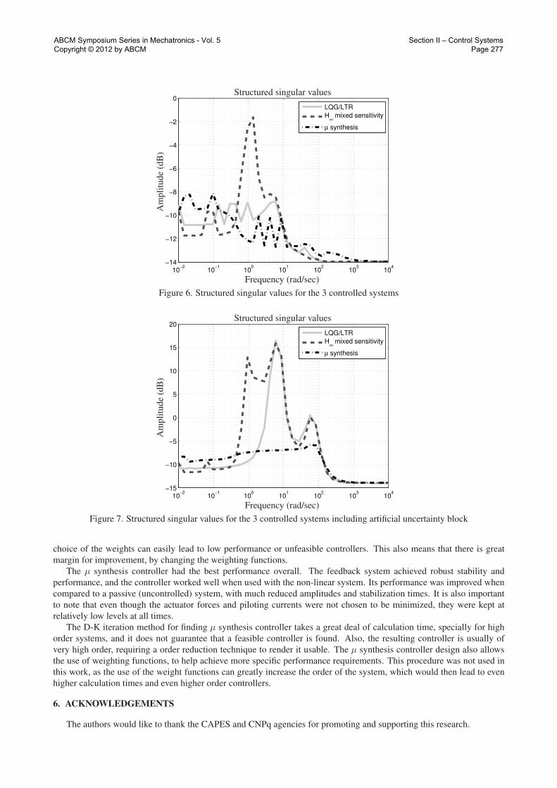
The structured singular values for the three systems, regarding the structured uncertainty described in Section 3.5 ,

were obtained and plotted on Figure 6. These values help determining the robust stability of the systems. It can be seen

that the robust stability conditions (µ∆ ≤ 1 (0dB)) is satisfied for all systems and for the whole frequency range.

To verify the robust performance of the systems, an artificial uncertainty block ∆p related to the performance vector zis added, thus creating a larger set of uncertainties. The structured singular values of the system for this new set (µ∆,∆p

)

was also calculated, and is shown on Figure 7. In this case, the only system that satisfies robust performance is the µsynthesis controller system.

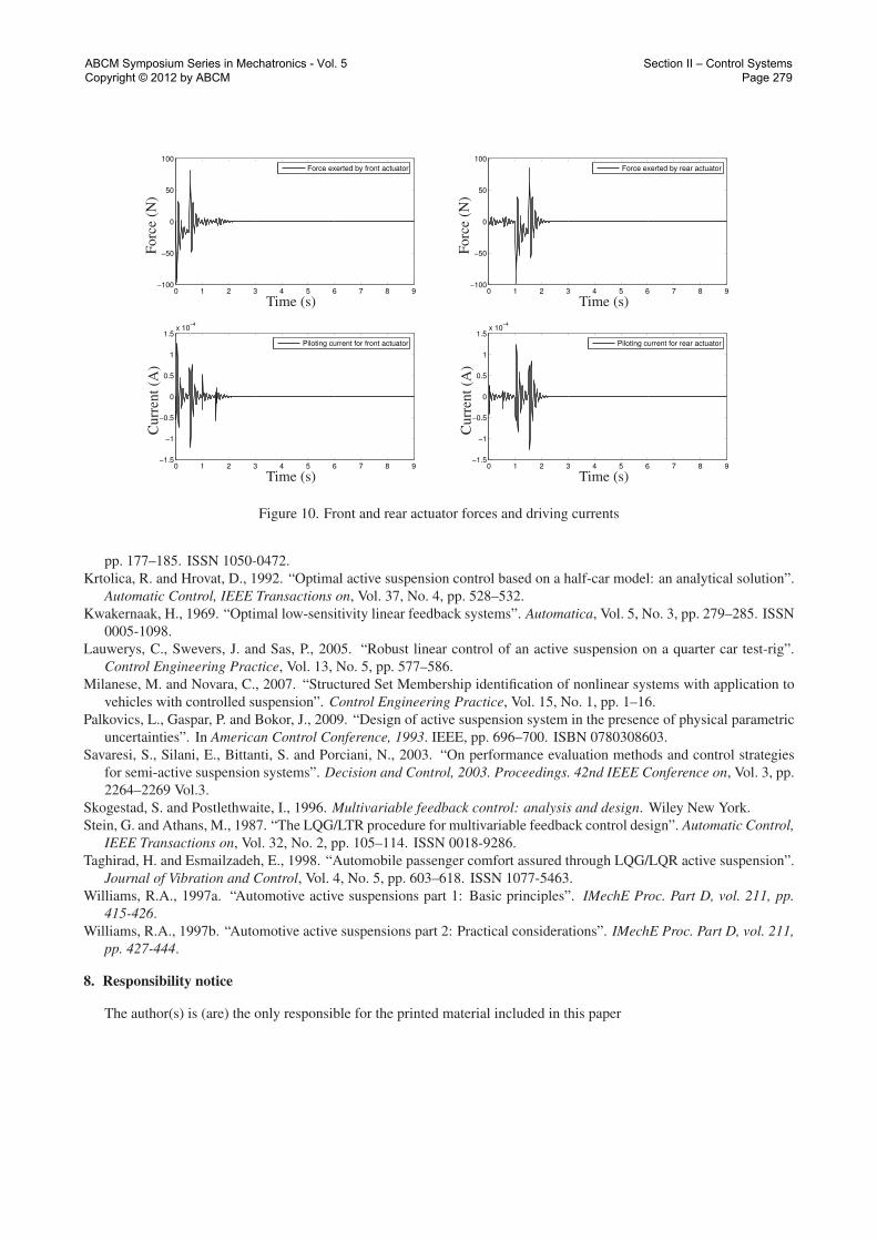
Finally, a non-linear model of the actuator, obtained in Engelman and Rizzoni (2009) was implemented using Simulink,

and the µ synthesis control was tested using the non-linear actuator and compared with an uncontrolled (passive) system.

An impulsive road profile was used, with an amplitude of 0.1 meters and a horizontal velocity of 60 Km/h is assumed,

and the simulation was carried for 9 seconds. The responses for θ, θ, z and z are shown on Figures 8(a), 8(b), 9(a) and

9(b), respectively. On Figure 10, the front and rear actuator forces and driving currents are shown.

5. CONCLUSION AND RESULTS ANALYSIS

Three robust control techniques, LQG/LTR, Mixed-sensitivity H∞ and µ synthesis, were investigated and designed

for use in an automotive active suspension system, represented using a half-car model and a hydraulic actuator model.

The LQG/LTR control was the simplest controller designed. Its design is basically straight forward, with few parame-

ters to be chosen. However, this simplicity also means that there is less improvement margin for the controller - not much

can be done if it does not satisfy the robustness requirements.

On the other hand, the Mixed-sensitivity H∞ was the most complex to be designed. The choice of the weighting

functions is a very complex and delicate procedure, specially in a MIMO system with so many inputs and outputs. The



10−2

10−1

100

101

102

103

104

−14

−12

−10

−8

−6

−4

−2

0

LQG/LTR

H∞

mixed sensitivity

µ synthesis

Frequency (rad/sec)

Am

pli

tude

(dB

)

Structured singular values

Figure 6. Structured singular values for the 3 controlled systems

10−2

10−1

100

101

102

103

104

−15

−10

−5

0

5

10

15

20

LQG/LTR

H∞

mixed sensitivity

µ synthesis

Frequency (rad/sec)

Am

pli

tude

(dB

)

Structured singular values

Figure 7. Structured singular values for the 3 controlled systems including artificial uncertainty block

choice of the weights can easily lead to low performance or unfeasible controllers. This also means that there is great

margin for improvement, by changing the weighting functions.

The µ synthesis controller had the best performance overall. The feedback system achieved robust stability and

performance, and the controller worked well when used with the non-linear system. Its performance was improved when

compared to a passive (uncontrolled) system, with much reduced amplitudes and stabilization times. It is also important

to note that even though the actuator forces and piloting currents were not chosen to be minimized, they were kept at

relatively low levels at all times.

The D-K iteration method for finding µ synthesis controller takes a great deal of calculation time, specially for high

order systems, and it does not guarantee that a feasible controller is found. Also, the resulting controller is usually of

very high order, requiring a order reduction technique to render it usable. The µ synthesis controller design also allows

the use of weighting functions, to help achieve more specific performance requirements. This procedure was not used in

this work, as the use of the weight functions can greatly increase the order of the system, which would then lead to even

higher calculation times and even higher order controllers.

6. ACKNOWLEDGEMENTS

The authors would like to thank the CAPES and CNPq agencies for promoting and supporting this research.



0 1 2 3 4 5 6 7 8 9−6

−4

−2

0

2

4

6x 10

−4

µ synthesis control with non−linear actuator

Passive

Am

pli

tude

(rad

)

Time (s)

Impulse response

(a) Impulse response of the pitch angle θ - comparison between µ

synthesis control using non-linear actuator and passive system

0 1 2 3 4 5 6 7 8 9−4

−3

−2

−1

0

1

2

3

4x 10

−3


Passive

Am

pli

tude

(rad

/s)

Time (s)

Impulse response

(b) Impulse response of the pitch velocity θ - comparison between µ

synthesis control using non-linear actuator and passive system

Figure 8. Impulse response of the pitch angle and velocity for active and passive systems

0 1 2 3 4 5 6 7 8 9−4

−2

0

2

4

6

8

10x 10

−4


Passive

Am

pli

tude

(m)

Time (s)

Impulse response

(a) Impulse response of the C.G vertical displacement z - compari-

son between µ synthesis control using non-linear actuator and passive

system

0 1 2 3 4 5 6 7 8 9−5

−4

−3

−2

−1

0

1

2

3

4

5x 10

−3


Passive

Am

pli

tude

(m/s

)

Time (s)

Impulse response

(b) mpulse response of the C.G vertical velocity z - comparison be-

tween µ synthesis control using non-linear actuator and passive sys-

tem

Figure 9. Impulse response of the center of gravity displacement and velocity for the active and passive systems

7. REFERENCES

Canale, M., Milanese, M. and Novara, C., 2006. “Semi-active suspension control using fast model-predictive techniques”.

Control Systems Technology, IEEE Transactions on, Vol. 14, No. 6, pp. 1034–1046.

D. Karnopp, M.J. Crosby, R.H., 1974. “Vibration control using semi-active force generators”. ASME - Journal of

Engineering for Industry.

Doyle, J., 1985. “Structured uncertainty in control system design”. In Decision and Control, 1985 24th IEEE Conference

on. IEEE, Vol. 24, pp. 260–265.

Du, H., Sze, K.Y. and Lam, J., 2005. “Semi-active h-infinity control of vehicle suspension with magneto-rheological

dampers”. Journal of Sound and Vibration, Vol. 283, No. 3-5, pp. 981–996.

Engelman, G. and Rizzoni, G., 2009. “Including the force generation process in active suspension control formulation”.

In American Control Conference, 1993. IEEE, pp. 701–705.

Fischer, D. and Isermann, R., 2004. “Mechatronic semi-active and active vehicle suspensions”. Control Engineering

Practice, Vol. 12, No. 11, pp. 1353–1367.

Gu, D., Petkov, P. and Konstantinov, M., 2005. Robust control design with MATLAB. Springer Verlag.

Herrnberger, M., M

"ader, D. and Lohmann, B., 2008. “Linear Robust Control for a Nonlinear Active Suspension Model Considering

Variable Payload”. Proceedings of the 17th IFAC World Congress (WC), Seoul, South Korea.

Hrovat, D., 1993. “Applications of Optmal-control to Advanced Automotive Suspension Design”. Journal of Dynamic

Systems Measurement and Control-Transactions of the ASME, Vol. 115, No. 2B, pp. 328–342. ISSN 0022-0434.

Karnopp, D., 1995. “Active and Semiactive Vibration Isolation”. Journal of Mechanical Design, Vol. 117, No. Sp. Iss. B,



0 1 2 3 4 5 6 7 8 9−100

−50

0

50

100

Force exerted by front actuator

0 1 2 3 4 5 6 7 8 9−100

−50

0

50

100

Force exerted by rear actuator

0 1 2 3 4 5 6 7 8 9−1.5

−1

−0.5

0

0.5

1

1.5x 10

−4

Piloting current for front actuator

0 1 2 3 4 5 6 7 8 9−1.5

−1

−0.5

0

0.5

1

1.5x 10

−4

Piloting current for rear actuator

Forc

e(N

)

Time (s)

Forc

e(N

)

Time (s)

Curr

ent

(A)

Time (s)C

urr

ent

(A)

Time (s)

Figure 10. Front and rear actuator forces and driving currents

pp. 177–185. ISSN 1050-0472.

Krtolica, R. and Hrovat, D., 1992. “Optimal active suspension control based on a half-car model: an analytical solution”.

Automatic Control, IEEE Transactions on, Vol. 37, No. 4, pp. 528–532.

Kwakernaak, H., 1969. “Optimal low-sensitivity linear feedback systems”. Automatica, Vol. 5, No. 3, pp. 279–285. ISSN

0005-1098.

Lauwerys, C., Swevers, J. and Sas, P., 2005. “Robust linear control of an active suspension on a quarter car test-rig”.

Control Engineering Practice, Vol. 13, No. 5, pp. 577–586.

Milanese, M. and Novara, C., 2007. “Structured Set Membership identification of nonlinear systems with application to

vehicles with controlled suspension”. Control Engineering Practice, Vol. 15, No. 1, pp. 1–16.

Palkovics, L., Gaspar, P. and Bokor, J., 2009. “Design of active suspension system in the presence of physical parametric

uncertainties”. In American Control Conference, 1993. IEEE, pp. 696–700. ISBN 0780308603.

Savaresi, S., Silani, E., Bittanti, S. and Porciani, N., 2003. “On performance evaluation methods and control strategies

for semi-active suspension systems”. Decision and Control, 2003. Proceedings. 42nd IEEE Conference on, Vol. 3, pp.

2264–2269 Vol.3.

Skogestad, S. and Postlethwaite, I., 1996. Multivariable feedback control: analysis and design. Wiley New York.

Stein, G. and Athans, M., 1987. “The LQG/LTR procedure for multivariable feedback control design”. Automatic Control,

IEEE Transactions on, Vol. 32, No. 2, pp. 105–114. ISSN 0018-9286.

Taghirad, H. and Esmailzadeh, E., 1998. “Automobile passenger comfort assured through LQG/LQR active suspension”.

Journal of Vibration and Control, Vol. 4, No. 5, pp. 603–618. ISSN 1077-5463.

Williams, R.A., 1997a. “Automotive active suspensions part 1: Basic principles”. IMechE Proc. Part D, vol. 211, pp.

415-426.

Williams, R.A., 1997b. “Automotive active suspensions part 2: Practical considerations”. IMechE Proc. Part D, vol. 211,

pp. 427-444.

8. Responsibility notice

The author(s) is (are) the only responsible for the printed material included in this paper



comparison of robust control techniques … · comparison of robust control techniques for use in...

Documents