comparison of estimated areas contributing recharge to ... · spring using ground-water withdrawals...

Comparison of Estimated Areas Contributing Recharge to Selected Springs in North-Central Florida by Using Multiple Ground-Water Flow Models

By W. Barclay Shoemaker1, Andrew M. O’Reilly1, Nicasio Sepúlveda1, Stanley A. Williams2, Louis H. Motz3, and Qing Sun3

U.S. Geological Survey

Open-File Report 03-448

Prepared in cooperation with the

St. Johns River Water Management District and the Florida Department of Environmental Protection

1U.S. Geological Survey2St. Johns River Water Management District3University of Florida

Tallahassee, Florida2004

U.S. DEPARTMENT OF THE INTERIOR GALE A. NORTON, Secretary

U.S. GEOLOGICAL SURVEYCharles G. Groat, Director

Use of trade, product, or firm names in this publication is for descriptive purposes only and does not imply endorsement by the U.S. Geological Survey.

For additional information write to:

U.S. Geological Survey2010 Levy AvenueTallahassee, FL 32310

Copies of this report can be purchased from:

U.S. Geological SurveyBranch of Information ServicesBox 25286Denver, CO 80225-0286888-ASK-USGS

Additional information about water resources in Florida is available on the internet at http://fl.water.usgs.gov

CONTENTS

Abstract ................................................................................................................................................................................. 1Introduction........................................................................................................................................................................... 1 Purpose and Scope ....................................................................................................................................................... 2 Hydrogeologic Setting ................................................................................................................................................. 2 Acknowledgments........................................................................................................................................................ 7Description of Ground-Water Flow Models ......................................................................................................................... 7 Peninsular Florida Model............................................................................................................................................. 7 Lake County/Ocala National Forest Model ................................................................................................................. 9 North-Central Florida Model ....................................................................................................................................... 10 Volusia County Model .................................................................................................................................................. 10Estimation of Areas Contributing Recharge ......................................................................................................................... 11 Description of Particle-Tracking Analyses .................................................................................................................. 11 Areas Contributing Recharge....................................................................................................................................... 14

Blue Spring ...................................................................................................................................................... 15 Silver Springs ................................................................................................................................................... 20 Alexander Springs............................................................................................................................................ 23 Silver Glen Springs .......................................................................................................................................... 23 Effects of Projected 2020 Ground-Water Withdrawals ................................................................................... 28

Limitations .................................................................................................................................................................... 28Summary ............................................................................................................................................................................... 29References............................................................................................................................................................................. 30Appendix 1............................................................................................................................................................................ disc

FIGURES

1. Map showing extent of the study area, ground-water flow models, and location of springs, north-central Florida ................................................................................................................................................ 3

2. Chart showing summary of hydrogeologic units in the study area .......................................................................... 43. Map showing estimated potentiometric surface of the Upper Floridan aquifer, average conditions for

August 1993 through July 1994 ............................................................................................................................... 64. Map showing areas contributing recharge to Blue Spring based on travel times up to 100 years as

simulated by Lake County/Ocala National Forest; Peninsular Florida; Volusia County models for the average hydrologic conditions of the calibration period; and composite area for all three models. ............ 16

5. Graph showing particle travel time as a percentage of total spring discharge to Blue Spring based on average hydrologic conditions of the calibration period.......................................................................................... 17

6. Diagram showing path lines along section A-A' for Blue Spring and contributing recharge areas based on travel times up to 100 years, as simulated by the Volusia County model for average 1995 hydrologic conditions............................................................................................................................................... 18

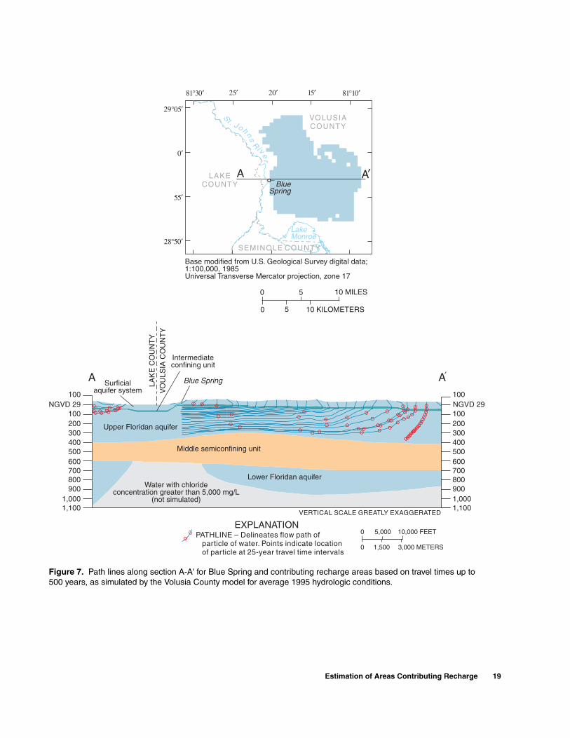
7. Diagram showing path lines along section A-A' for Blue Spring and contributing recharge areas based on travel times up to 500 years, as simulated by the Volusia County model for average 1995 hydrologic conditions............................................................................................................................................... 19

8. Map showing areas contributing recharge to Silver Springs based on travel times up to 100 years as simulated by Lake County/Ocala National Forest; Peninsular Florida; North-Central Florida models for the average hydrologic conditions of the calibration period; and composite area for all three models................... 21

9. Graph showing particle travel time as a percentage of total spring discharge to Silver Springs based on average hydrologic conditions of the calibration period..................................................................................... 22

Contents III

10. Map showing areas contributing recharge to Alexander Springs based on travel times up to 100 years as simulated by Lake County/Ocala National Forest; Peninsular Florida; North-Central Florida models for the average hydrologic conditions of the calibration period; and composite area for all three models .................. 24

11. Graph showing particle travel time as a percentage of total spring discharge to Alexander Springs based on average hydrologic conditions of the calibration period .......................................................................... 25

12. Map showing areas contributing recharge to Silver Glen Springs based on travel times up to 100 years as simulated by Lake County/Ocala National Forest; Peninsular Florida; North-Central Florida models for the average hydrologic conditions of the calibration period; and composite area for all three models .................. 26

13. Graph showing particle travel time as a percentage of total spring discharge to Silver Glen Springs based on average hydrologic conditions of the calibration period .................................................................................... 27

TABLES

1. Summary of models and springs for which areas contributing recharge were delineated...................................... 22. Simulated spring discharges for the ground-water flow models at selected springs .............................................. 53. Summary of features for the ground-water flow models ........................................................................................ 84. Parameter value statistics from the calibrated ground-water flow models for the areas contributing

recharge to selected springs delineated by each model based on travel times up to 100 years and average hydrologic conditions of the calibration period......................................................................................... 14

IV Contents

CONVERSION FACTORS, DATUMS, ACRONYMS, AND ABBREVIATIONS

*The standard unit for transmissivity is cubic foot per day per square foot times foot of aquifer thickness [(ft3/d)/ft2]ft. In this report, the mathematically reduced form, foot squared per day (ft2/d), is used for convenience.

Temperature in degrees Fahrenheit (°F) may be converted to degrees Celsius (°C) as follows: C=(°F-32)/1.8.

Vertical coordinate information is referenced to the National Geodetic Vertical Datum of 1929 (NGVD 29).

Horizontal coordinate information (latitude-longitude) is referenced to the North American Datum of 1927 (NAD27).

Acronyms and abbreviations:

FDEP Florida Department of Environmental Protection

FAS Floridan aquifer system

GIS Geographic Information System

IAS intermediate aquifer system

ICU intermediate confining unit

PF model Peninsular Florida model

LCONF model Lake County/Ocala National Forest model

LFA Lower Floridan aquifer

MCU middle confining unit

MSCU middle semiconfining unit

mg/L milligrams per liter

NCF model North-Central Florida model

SAS surficial aquifer system

SFCU sub-Floridan confining unit

UFA Upper Floridan aquifer

VC model Volusia County model

Multiply By To obtain

Lengthinch (in.) 2.54 centimeter

foot (ft) 0.3048 metermile (mi) 1.609 kilometer

Areasquare mile (mi2) 2.590 square kilometer

Flow Ratecubic foot per second (ft3/s) 0.02832 cubic meter per second

cubic foot per day (ft3/d) 0.02832 cubic meter per daymillion gallons per day (Mgal/d) 0.04381 cubic meter per second

inch per year (in/yr) 25.4 millimeter per year

Hydraulic Conductivityfoot per day (ft/d) 0.3048 meter per day

*Transmissivityfoot squared per day (ft2/d) 0.09290 meter squared per day

Leakancefoot per day per foot [(ft/d)/ft] 1.0 meter per day per meter

Contents V

VI Contents

Comparison of Estimated Areas Contributing Recharge to Selected Springs in North-Central Florida by Using Multiple Ground-Water Flow ModelsBy W. Barclay Shoemaker, Andrew M. O’Reilly, Nicasio Sepúlveda, Stanley A. Williams, Louis H. Motz, and Qing Sun

ABSTRACT

Areas contributing recharge to springs are defined in this report as the land-surface area wherein water entering the ground-water system at the water table eventually discharges to a spring. These areas were delineated for Blue Spring, Silver Springs, Alexander Springs, and Silver Glen Springs in north-central Florida using four regional ground-water flow models and particle tracking. As expected, different models predicted different areas contributing recharge. In general, the differences were due to different hydrologic stresses, subsurface permeability properties, and boundary conditions that were used to calibrate each model, all of which are con-sidered to be equally feasible because each model matched its respective calibration data reasonably well. To evaluate the agreement of the models and to summarize results, areas contributing recharge to springs from each model were combined into composite areas. During 1993-98, the composite areas contributing recharge to Blue Spring, Silver Springs, Alexander Springs, and Silver Glen Springs were about 130, 730, 110, and 120 square miles, respectively. The composite areas for all springs remained about the same when using projected 2020 ground-water withdrawals.

INTRODUCTION

Springs are an important water resource to be protected by the State of Florida, particularly in parts of north-central Florida where many of the State’s most productive springs are located. Springs are important because they (1) contribute freshwater to sensitive ecosystems where many biological commu-nities reside; (2) provide a resource for recreational activities; and (3) contribute to local economies when, for example, they are used as recreation sites or as a source for bottled water. Springs also are indicators of the health of the ground-water system. That is, springs generally reflect the prevailing conditions affecting the aquifer, whether it is a drought or excessive ground-water withdrawals causing a reduction in spring flow or land-use practices such as farming or urban devel-opment causing a degradation in spring water quality. Considering the importance of springs, the Florida Department of Environmental Protection (FDEP) wants to define the areas contributing recharge to springs for regulatory and planning purposes.

Areas contributing recharge to springs are defined in this report as the land-surface area wherein water entering the ground-water system at the water table eventually discharges to a spring (Reilly and Pollock, 1993). Previous investigations have described methods to delineate areas contributing recharge to various hydrologic features. For example, Reilly and Pollock (1993) discussed the factors that affect areas contributing recharge to wells in shallow aquifers. In Cape Cod, Massachusetts, areas contributing recharge to existing and hypothetical public supply wells were

Abstract 1

delineated (Barlow, 1994a, 1994b). Masterson and Walter (2000) and Masterson and others (2002) also delineated areas contributing recharge to local bays, canals, sounds, ponds, streams, and pumping wells in western Cape Cod, Massachusetts. Renken and others (2001) developed an approach for identifying areas contributing recharge to municipal supply wells using telescopic mesh refinement, particle tracking, geo-graphic information systems, and a graphical user interface. In north-central Florida, Murray and Halford (1996) and Knowles and others (2002) delineated areas contributing recharge to several springs and well fields.

Purpose and Scope

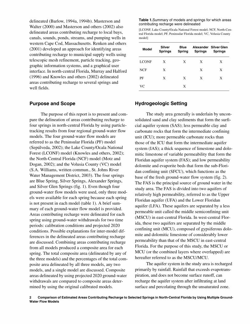
The purpose of this report is to present and com-pare the delineation of areas contributing recharge to four springs in north-central Florida by using particle-tracking results from four regional ground-water flow models. The four ground-water flow models are referred to as the Peninsular Florida (PF) model (Sepúlveda, 2002); the Lake County/Ocala National Forest (LCONF) model (Knowles and others, 2002); the North-Central Florida (NCF) model (Motz and Dogan, 2002); and the Volusia County (VC) model (S.A. Williams, written commun., St. Johns River Water Management District, 2003). The four springs are Blue Spring, Silver Springs, Alexander Springs, and Silver Glen Springs (fig. 1). Even though four ground-water flow models were used, only three mod-els were available for each spring because each spring is not present in each model (table 1). A brief sum-mary of each ground-water flow model is provided. Areas contributing recharge were delineated for each spring using ground-water withdrawals for two time periods: calibration conditions and projected 2020 conditions. Possible explanations for inter-model dif-ferences in the delineated areas contributing recharge are discussed. Combining areas contributing recharge from all models produced a composite area for each spring. The total composite area (delineated by any of the three models) and the percentages of the total com-posite area delineated by all three models, any two models, and a single model are discussed. Composite areas delineated by using projected 2020 ground-water withdrawals are compared to composite areas deter-mined by using the original calibrated models.

2 Comparison of Estimated Areas Contributing Recharge to SeWater Flow Models

Hydrogeologic Setting

The study area generally is underlain by uncon-solidated sand and clay sediments that form the surfi-cial aquifer system (SAS); less permeable clay and carbonate rocks that form the intermediate confining unit (ICU); more permeable carbonate rocks than those of the ICU that form the intermediate aquifer system (IAS); a thick sequence of limestone and dolo-mitic limestone of variable permeability that form the Floridan aquifer system (FAS); and low permeability dolomite and evaporite beds that form the sub-Flori-dan confining unit (SFCU), which functions as the base of the fresh ground-water flow system (fig. 2). The FAS is the principal source of ground water in the study area. The FAS is divided into two aquifers of relatively high permeability, referred to as the Upper Floridan aquifer (UFA) and the Lower Floridan aquifer (LFA). These aquifers are separated by a less permeable unit called the middle semiconfining unit (MSCU) in east-central Florida. In west-central Flor-ida, these two aquifers are separated by the middle confining unit (MCU), composed of gypsiferous dolo-mite and dolomitic limestone of considerably lower permeability than that of the MSCU in east-central Florida. For the purpose of this study, the MSCU or MCU (or the combined layers where overlapped) are hereafter referred to as the MSCU/MCU.

The aquifer system in the study area is recharged primarily by rainfall. Rainfall that exceeds evapotrans-piration, and does not become surface runoff, can recharge the aquifer system after infiltrating at land surface and percolating through the unsaturated zone.

Table 1.Summary of models and springs for which areas contributing recharge were delineated

[LCONF, Lake County/Ocala National Forest model; NCF, North-Cen-tral Florida model; PF, Peninsular Florida model; VC, Volusia County model]

ModelSilver

SpringsBlue

SpringAlexander Springs

Silver Glen Springs

LCONF X X X X

NCF X X X

PF X X X X

VC X

lected Springs in North-Central Florida by Using Multiple Ground-

0

0 25

25

50 MILES

50 KILOMETERS

ATLA

NT

ICO

CE

AN

GU

LF

OF

ME

XIC

O

��

��

��

��

��

��

Base modified from U.S. Geological Survey digital data; 1:100,000, 1985Universal Transverse Mercator projection, zone 17

TAM

PABAY

Extent ofPeninsularFloridaModel

Orlando

Gainesville

St. Petersburg

Tampa

Live Oak Jacksonville

Ocala

Extent ofVolusiaCountyModel

Extent ofLake County/OcalaNational ForestModel

Extent ofNorth-CentralFloridaModel

PUTNAM

DUVAL

FLAGLERS

T. JOH

NS

BRADFORD

OSCEOLA

BAKER

BR

EVA

RD

INDIANRIVER

ST. LUCIE

MARTIN

OKEECHOBEE

HIG

HLA

ND

S

GLADES

HARDEE

DE SOTO

CHARLOTTE

SARASOTA

MANATEE

HILLSBOROUGHPIN

ELLA

S

PASCO

HERNANDO

CITRUS

ALACHUA

LEVY

DIXIE

GILC

HR

IST

LAFAYETTE

UNION

COLUMBIASUWANNEE

MA

DIS

ON

HAMILTON

WARE

CHARLTON

NASSAU

CLAY

MARION

POLK

SUMTER

LAKE

SEMINOLE

ORANGE

VOLUSIA

FLORIDA

GEORGIA

CLINCH

ECHOLS

LOW

ND

ES

LANIER CAMDEN

PUTNAM

SilverSprings

Silver GlenSprings

AlexanderSprings

BlueSpring

STUDY AREA

The Everglades

Lake Okeechobee

GEORGIA

FLORIDA

Figure 1. Extent of the study area, ground-water flow models, and location of springs, north-central Florida.

Introduction 3

Sources of water to the aquifer system, in addition to net recharge from rainfall, are artificial recharge (for example, irrigation or rapid infiltration basins) and subsurface inflow from outside the study area. Inflow to the aquifer system in the study area is eventually discharged by springs, leakage to some surface-water bodies, wells, and subsurface outflow. For example, total inflow to the aquifer system simulated by the LCONF model was 13 inches per year (in/yr) averaged over the entire model area of approximately 4,800 square miles (mi2), 95 percent of which was net recharge from rainfall. This inflow was balanced by the following simulated outflows from the aquifer sys-tem: 6 in/yr of spring flow; 4 in/yr of leakage from the aquifer system to streams, lakes, or wetlands; 2 in/yr

of pumpage; and 1 in/yr of subsurface flow across model boundaries (Knowles and others, 2002, p. 86).

Patterns of rainfall and evapotranspiration partly explain the occurrence and movement of ground water beneath north-central Florida. Rainfall in north-central Florida is highly variable both spatially and tempo-rally, with an annual average of about 51 inches (in.) (Knowles and others, 2002, p. 30). Convective storm events and squalls produce variable patterns of rain-fall, whereas rainfall from fronts, hurricanes, and trop-ical depressions generally is more uniform and widespread. Evapotranspiration depletes much of the rainfall available for ground-water recharge by direct evaporation and transpiration. Knowles (1996) and Sumner (2001) evaluated the processes that govern evapotranspiration in Florida. Knowles (1996)

SERIES LITHOLOGY HYDROGEOLOGICUNITS

STRATIGRAPHICUNIT

UNDIFFERENTIATEDDEPOSITS

HAWTHORNGROUP

OCALALIMESTONE

AVON PARKFORMATION

OLDSMARFORMATION

CEDAR KEYSFORMATION

HOLOCENE

PLEISTOCENE

PLIOCENE

MIOCENE

PALEOCENE

LOWER

MIDDLE

UPPER

EO

CE

NE

Alluvium, freshwater marl, peats and mudsin stream and lake bottoms. Also, somedunes and other windblown sand.

Mostly quartz sand. Locally can containorganic deposits and thin beds of clay.

Interbedded deposits of sand, silty sandand clay, shell fragments; phosphatic claysometimes present at base of formation.

Interbedded quartz, sand, silt, shell, and clay;green to gray and white, phosphatic,cemented alluvial conglomerate, sandstone,dolostone, and limestone; typically silicifiedand fractured near base of formation.

White to cream to tan, soft to hard, granular,porous, marine foraminiferal limestone, oftendolomitic; sometimes sand, sandy or chertylimestone at top of formation.

Light brown to brown, soft to hard, porous todense, granular to chalky, fossiliferouslimestone and brown, crystalline dolomite,locally contains some gypsum.

Alternating beds of light brown to white,chalky, porous, fossiliferous limestone andporous crystalline dolomite; minor amountsof anhydrite and gypsum.

Dolomite, with considerable anhydrite andgypsum, some limestone.

OLIGOCENE SUWANEELIMESTONE

Limestone, sandy limestone, fossiliferous

SURFICIALAQUIFERSYSTEM

SUB-FLORIDANCONFINING

UNIT

LOWERFLORIDANAQUIFER

MIDDLESEMICONFINING

UNIT

UPPERFLORIDANAQUIFER

INTERMEDIATECONFINING

UNIT

INTERMEDIATEAQUIFERSYSTEM

MIDDLECONFINING

UNIT

FLO

RID

AN

AQ

UIF

ER

SY

ST

EM

Figure 2. Summary of hydrogeologic units in the study area (modified from Knowles and others, 2002, and Sepúlveda, 2002).

4 Comparison of Estimated Areas Contributing Recharge to Selected Springs in North-Central Florida by Using Multiple Ground-Water Flow Models

estimated evapotranspiration rates of about 38 in/yr by using a water budget approach over a 30-year period from 1965 to 1994 in the Silver Springs ground-water basin. Sumner (2001) estimated average annual evapo-transpiration rates of about 36 in. and 42 in. for 1998 and 1999, respectively, at a single evapotranspiration measurement station over pine flat wood uplands interspersed within cypress wetlands in Volusia County.

In a geologic setting where limestone is at or near land surface, net recharge interacts with the car-bonate rocks, resulting in karst terrain. Karst is charac-terized by the absence of a well-defined surface drainage system and is drained internally, that is, rainfall not lost to evapotranspiration infiltrates and recharges the aquifer. Internal drainage results in higher net recharge rates, which are conducive to the dissolution of limestone and the formation of such features as voids and conduits in the limestone and closed depressions at land surface. In locations where the potentiometric surface of the FAS is above land surface, ground water may discharge as diffuse upward flow through the ICU or as discrete discharge through breaches in the ICU. Such locations of dis-crete discharge are called springs.

Springs in Florida are categorized by their long-term mean ground-water discharge (Rosenau and others, 1977). The largest springs in the study area discharge ground water at rates of 100 cubic feet

per second (ft3/s) or greater, and are referred to as first-magnitude springs. Areas contributing recharge were delineated for first-magnitude springs only, all of which discharge ground water from the UFA. Long-term average discharges reported by Knowles and oth-ers (2002, p. 36-37) for the springs are given in table 2. Together, these four springs discharge ground water at a rate of about 740 million gallons per day (Mgal/d).

Ground-water pumpage is another source of discharge from the FAS. Ground-water pumpage has increased steadily for several decades in response to demands from a growing population. Meanwhile, spring discharge has generally declined slightly since 1940, as have water levels in north-central Florida lakes, streams, wetlands, the SAS, and FAS (Knowles and others, 2002). Although much of the decline can be attributed to below-average rainfall, increased pumpage is likely a contributing factor.

Areas contributing recharge to springs can be approximated by mapping potentiometric surface con-tours. For example, the average potentiometric surface of the UFA during 1993-1994 (fig. 3) can be used to delineate areas contributing recharge to springs if flow is assumed to be two-dimensional. However, the effect of three-dimensional flow in a layered aquifer system such as the FAS is difficult to ascertain based only on potentiometric surface contours. Ground-water flow models can account for vertical flow and, therefore, were used in this study.

Table 2. Simulated spring discharges for the ground-water flow models at selected springs

[LT Av., long-term average reported by Knowles and others (2002, p. 36-37); Cal., calibrated; discharge in cubic feet per second; LCONF, Lake County/Ocala National Forest model; NCF, North-Central Florida model; PF, Peninsular Florida model; VC, Volusia County model; --, spring not simulated]

Models

Silver Springs Blue Spring Alexander Springs Silver Glen Springs

LT Av.

Cal. 2020LT Av.

Cal. 2020LT Av.

Cal. 2020LT Av.

Cal. 2020

LCONFa 788 920 889 156 164 159 106 104 103 102 102 102

NCFb 788 678 625 -- --e --e 106 90 90 102 88 88

PFc 788 620 571 156 126 111 106 102 101 102 79 78

VCd -- -- -- 156 149 138 -- -- -- -- -- --

aCalibration period average 1998.bCalibration period May 1995.cCalibration period average 1993-94.dCalibration period average 1995.eDischarge data not reported because only 20 percent of spring discharge was simulated due to proximity of Blue Spring to the eastern

model boundary (Motz and Dogan, 2002).

Introduction 5

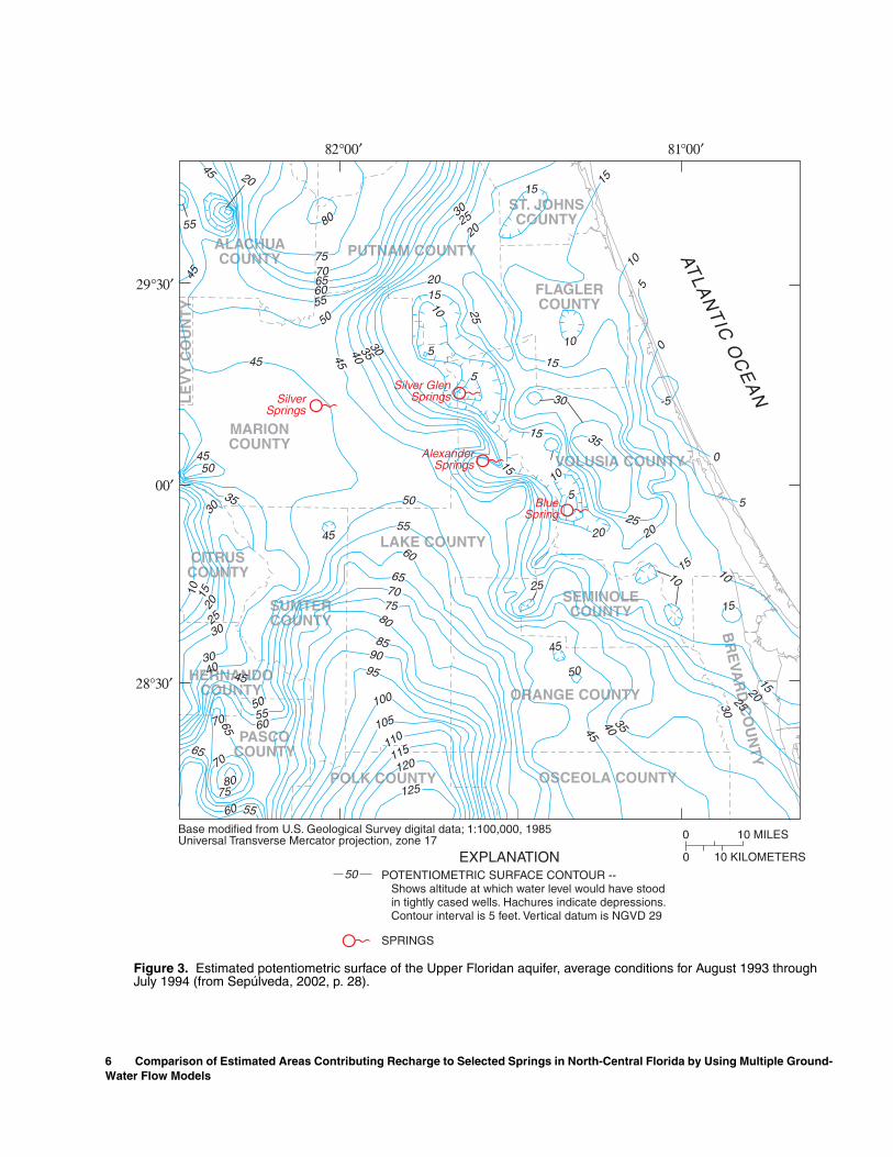
EXPLANATIONPOTENTIOMETRIC SURFACE CONTOUR --

Shows altitude at which water level would have stoodin tightly cased wells. Hachures indicate depressions.Contour interval is 5 feet. Vertical datum is NGVD 29

50

SPRINGS

ALACHUACOUNTY PUTNAM COUNTY

ST. JOHNSCOUNTY

MARIONCOUNTY

FLAGLERCOUNTY

VOLUSIA COUNTY

SEMINOLECOUNTY

BR

EVA

RD

CO

UN

TY

LAKE COUNTY

ORANGE COUNTY

SUMTERCOUNTY

CITRUSCOUNTY

HERNANDOCOUNTY

PASCOCOUNTY

OSCEOLA COUNTY

ATLA

NT

ICO

CE

AN

POLK COUNTY

LE

VY

CO

UN

TY

10

15

5

125

120115110

105

100

95

9085

80757065

60

55

50

50

45

25

20

5

2520

1510

10

15

15202530

354045

5

0

-5

0

30

3515

1015

515

103035404545

4550

3530

45

10 15

20

2530

3040

45

505560

80

5055

45

60657075

2015

10

5

25

80

2045

553025

20

15

5560

65

6570

75

70

��

��


��

��

0

0 10 MILES

10 KILOMETERS

SilverSprings

Silver GlenSprings

BlueSpring

AlexanderSprings

Figure 3. Estimated potentiometric surface of the Upper Floridan aquifer, average conditions for August 1993 through July 1994 (from Sepúlveda, 2002, p. 28).


Acknowledgments

Trudy G. Phelps of the U.S. Geological Survey, Altamonte Springs, Florida, provided valuable project guidance and report review comments. Keith J. Halford of the U.S. Geological Survey, Carson City, Nevada, conducted backward particle-tracking analyses and created summary spreadsheets. Hal Davis of the U.S. Geological Survey, Tallahassee, Florida; Richard Lindgren of the U.S. Geological Survey, San Antonio, Texas; and Mark Zucker of the U.S. Geological Survey, Miami, Florida, provided useful review comments.

DESCRIPTION OF GROUND-WATER FLOW MODELS

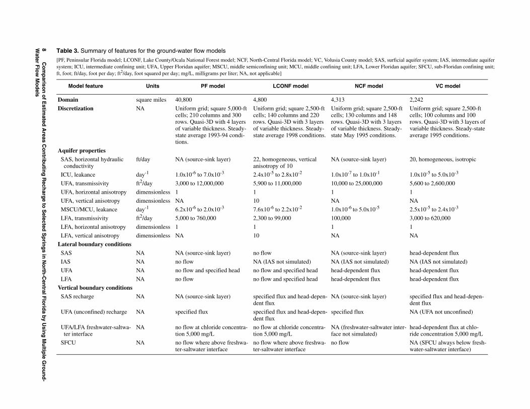
The four ground-water flow models used in this study were constructed by using the U.S. Geological Survey three-dimensional ground-water flow model code MODFLOW (McDonald and Harbaugh, 1988; Harbaugh and McDonald, 1996; Harbaugh and others, 2000). The models are described briefly in the follow-ing sections. The descriptions begin with a statement of the name and purpose of the model and a discussion of the extent and discretization of the model grid. Important hydraulic properties are summarized and followed by a brief discussion of boundary conditions. The observation types used to calibrate each model are mentioned briefly. Finally, the simulated effects of 2020 ground-water withdrawals on spring discharge are presented. Ground-water withdrawal rates for 2020 were estimated by the respective water management districts. For convenience, important details of each model also are summarized in table 3. For additional details not discussed below, the reader is referred to the cited reference for each model.

Peninsular Florida Model (PF Model)

The PF model (Sepúlveda, 2002) is a four-layer, steady-state ground-water flow model that includes most of peninsular Florida (fig. 1). The model simu-lates the SAS (layer 1) as a source-sink layer using specified heads. The model simulates water levels in the IAS in southwest Florida (layer 2), UFA (layer 3), and LFA (layer 4). Where present, the ICU was simu-lated by the leakances between layers 1 and 2 and between layers 2 and 3. The MSCU/MCU was simu-lated by the leakances between layers 3 and 4. Simula-tions were made to predict water-level declines from 1993–94 to 2020.

The PF model has the largest spatial extent of the four models used in this study (fig. 1). The active model area covers about 40,800 mi2, and extends northward to Charlton and Camden Counties, Georgia, and southward to just south of the Palm Beach - Mar-tin County line. From west-to-east, the model spans about 200 miles (mi) from the Gulf of Mexico to the Atlantic Ocean. The SAS was not included in areas where the UFA is unconfined. Vertically, the model extends to depths containing water with chloride con-centrations less than 5,000 milligrams per liter (mg/L). A uniform finite-difference grid of square 2,500-foot (ft) cells with 210 columns and 300 rows was employed.

The important hydraulic properties of the PF model include the leakance terms of the ICU and MSCU/MCU, as well as the transmissivity of the UFA and LFA (table 3). These parameters partly control the exchange of ground water between the SAS and FAS, and within the FAS, respectively, and horizontal ground-water flow within the FAS. The leakance of the ICU is heterogeneous, with values ranging from 1.0x10-6 to 7.0x10-3 day-1. The leakance of the MSCU/MCU is heterogeneous, with values ranging from 6.2x10-6 to 2.0x10-3 day-1. The transmissivity of the UFA is heterogeneous and isotropic, with values ranging from 3,000 to 12,000,000 feet squared per day (ft2/d). The transmissivity of the LFA is heterogeneous and isotropic, with values ranging from 5,000 to 760,000 ft2/d.

Boundary conditions for the PF model include specified fluxes, specified heads, and head-dependent fluxes (table 3). Specified-flux boundaries represented net recharge where the UFA is unconfined. Specified fluxes also represented wells withdrawing ground water used for public supply, agriculture, commercial or industrial purposes, and domestic self-supply. A special case of the specified-flux boundary is a no-flow boundary. No-flow boundaries at the base of the model represented the transition zone between fresh-water and saltwater at depth in the FAS because flow across this transition is likely negligible (Kohout, 1960; Reilly, 2001). Also, no-flow boundaries were used at some lateral boundaries of the model grid in the UFA and LFA. Specified-head boundary condi-tions represented the water table in the SAS as a source-sink layer. Specified-head boundaries also were used at some lateral boundaries of the model grid in the FAS. The specified heads were adjusted for freshwater equivalence at locations where salinity was expected to affect ground-water density. Finally, head-dependent flux boundary conditions represented springs.

Description of Ground-Water Flow Models 7

urficial aquifer system; IAS, intermediate aquifer idan aquifer; SFCU, sub-Floridan confining unit;

VC model

2,242

00-ft 48

ayers eady-ns.

Uniform grid; square 2,500-ft cells; 100 columns and 100 rows. Quasi-3D with 3 layers of variable thickness. Steady-state average 1995 conditions.

20, homogeneous, isotropic

1.0x10-5 to 5.0x10-3

5,600 to 2,600,000

1

NA

2.5x10-5 to 2.4x10-3

3,000 to 620,000

1

NA

head-dependent flux

NA (IAS not simulated)

head-dependent flux

head-dependent flux

specified flux and head-depen-dent flux

NA (UFA not unconfined)

r inter- head-dependent flux at chlo-ride concentration 5,000 mg/L

NA (SFCU always below fresh-water-saltwater interface)

8

Co

mp

arison

of E

stimated

Areas C

on

tribu

ting

Rech

arge to

Selected

Sp

ring

s in N

orth

-Cen

tral Flo

rida b

y Usin

g M

ultip

le Gro

un

d-

Water F

low

Mo

dels

Table 3. Summary of features for the ground-water flow models

[PF, Peninsular Florida model; LCONF, Lake County/Ocala National Forest model; NCF, North-Central Florida model; VC, Volusia County model; SAS, ssystem; ICU, intermediate confining unit; UFA, Upper Floridan aquifer; MSCU, middle semiconfining unit; MCU, middle confining unit; LFA, Lower Florft, foot; ft/day, foot per day; ft2/day, foot squared per day; mg/L, milligrams per liter; NA, not applicable]

Model feature Units PF model LCONF model NCF model

Domain square miles 40,800 4,800 4,313

Discretization NA Uniform grid; square 5,000-ft cells; 210 columns and 300 rows. Quasi-3D with 4 layers of variable thickness. Steady-state average 1993-94 condi-tions.

Uniform grid; square 2,500-ft cells; 140 columns and 220 rows. Quasi-3D with 3 layers of variable thickness. Steady-state average 1998 conditions.

Uniform grid; square 2,5cells; 130 columns and 1rows. Quasi-3D with 3 lof variable thickness. Ststate May 1995 conditio

Aquifer properties

SAS, horizontal hydraulic conductivity

ft/day NA (source-sink layer) 22, homogeneous, vertical anisotropy of 10

NA (source-sink layer)

ICU, leakance day-1 1.0x10-6 to 7.0x10-3 2.4x10-5 to 2.8x10-2 1.0x10-7 to 1.0x10-1

UFA, transmissivity ft2/day 3,000 to 12,000,000 5,900 to 11,000,000 10,000 to 25,000,000

UFA, horizontal anisotropy dimensionless 1 1 1

UFA, vertical anisotropy dimensionless NA 10 NA

MSCU/MCU, leakance day-1 6.2x10-6 to 2.0x10-3 7.6x10-6 to 2.2x10-2 1.0x10-6 to 5.0x10-5

LFA, transmissivity ft2/day 5,000 to 760,000 2,300 to 99,000 100,000

LFA, horizontal anisotropy dimensionless 1 1 1

LFA, vertical anisotropy dimensionless NA 10 NA

Lateral boundary conditions

SAS NA NA (source-sink layer) no flow NA (source-sink layer)

IAS NA no flow NA (IAS not simulated) NA (IAS not simulated)

UFA NA no flow and specified head no flow and specified head head-dependent flux

LFA NA no flow no flow and specified head head-dependent flux

Vertical boundary conditions SAS recharge NA NA (source-sink layer) specified flux and head-depen-

dent fluxNA (source-sink layer)

UFA (unconfined) recharge NA specified flux specified flux and head-depen-dent flux

specified flux

UFA/LFA freshwater-saltwa-ter interface

NA no flow at chloride concentra-tion 5,000 mg/L

no flow at chloride concentra-tion 5,000 mg/L

NA (freshwater-saltwateface not simulated)

SFCU NA no flow where above freshwa-ter-saltwater interface

no flow where above freshwa-ter-saltwater interface

no flow

The PF model was calibrated to time-averaged hydrologic conditions from August 1993 through July 1994. A total of 1,780 observations were used for calibration. This included 1,624 hydraulic-head obser-vations representing water levels in the FAS, and 156 flow observations representing spring discharge or base flow to some surface-water features. Hydraulic properties and net recharge to unconfined areas of the UFA were adjusted until a reasonable fit between observations and simulated equivalents was obtained. The change in spring discharge from 1993-94 to 2020 as a result of projected ground-water withdrawals was computed. Spring discharge either remained about the same or decreased (table 2).

Lake County/Ocala National Forest Model (LCONF Model)

The LCONF model (Knowles and others, 2002) is a three-layer, steady-state ground-water flow model for Lake County, the Ocala National Forest, and adja-cent areas (fig. 1). The LCONF model simulates water levels in the SAS (layer 1), UFA (layer 2), and LFA (layer 3). The ICU and the MSCU/MCU were simu-lated by the leakances between layers 1 and 2 and between layers 2 and 3, respectively. Simulations were made to predict water-level declines from 1998 to 2020.

The active model area in the UFA covers about 4,800 mi2 in central and north-central Florida and extends from Putnam and Alachua Counties in the north to northern Polk and Osceola Counties in the south (fig. 1). The west-to-east extent of the model area spans about 65 mi from eastern Citrus and Her-nando Counties to central Volusia County. The SAS was not included in areas where the UFA is uncon-fined. The finite-difference grid used for the ground-water flow model was uniform and composed of square 2,500-ft cells, with 140 columns and 220 rows.

Important hydraulic properties in the LCONF model include the leakance terms of the ICU and MSCU/MCU, as well as the hydraulic conductivity of the SAS and transmissivity of the UFA and LFA (table 3). The leakance of the ICU is heterogeneous, with values ranging from 2.4x10-5 to 2.8x10-2 day-1 (Knowles and others, 2002, p. 76). The leakance of the

MSCU/MCU is heterogeneous, with values ranging from 7.6x10-6 to 2.2x10-2 day-1 (Knowles and others, 2002, p. 77). The hydraulic conductivity of the SAS is homogeneous, horizontally isotropic, and vertically anisotropic. A value of 22 ft/d was estimated for the hydraulic conductivity, and the vertical anisotropy ratio was set to 10. The transmissivity of the UFA is heterogeneous, horizontally isotropic, and vertically anisotropic. Transmissivity values range from 5,900 to 11,000,000 ft2/d. The vertical anisotropy ratio was set to 10. The transmissivity of the LFA also is heteroge-neous, horizontally isotropic, and vertically anisotro-pic. These transmissivity values range from 2,300 to 99,000 ft2/d. The vertical anisotropy ratio also was set to 10 for the LFA.

Boundary conditions for the LCONF model include specified fluxes, specified heads, and head-dependent fluxes (table 3). A combination of speci-fied-fluxes and head-dependent flux boundaries repre-senting net recharge served as the upper boundary condition, which was located at the altitude of the water table. Specified fluxes also represented wells withdrawing ground water used for public supply, agriculture, commercial or industrial purposes, and domestic self-supply. No-flow boundaries were estab-lished at the base of the model and at lateral bound-aries of the SAS and FAS. No-flow boundaries at the base of the model were established along the transition zone between freshwater and saltwater (chloride con-centrations greater than 5,000 mg/L), or at the base of the FAS, whichever occurred at a shallower depth. No-flow boundaries in the SAS were specified at the cells along the lateral boundaries of the model because rela-tively little lateral flow occurs in the SAS. No-flow boundaries also were established in the UFA and LFA where ground-water flow is perpendicular to model boundaries, based on potentiometric contour lines from the May 1998 UFA potentiometric-surface map. Along remaining lateral boundaries of the model, specified-head boundaries were used in the UFA and LFA from southwestern Marion to west-central Sumter Counties and across central Orange County. Head-dependent flux boundary conditions represented springs and the interaction of the ground-water system with streams, lakes, or wetlands.

The LCONF model was calibrated by using the inverse modeling capabilities of MODFLOW-2000

Description of Ground-Water Flow Models 9

(Hill and others, 2000). A total of 405 observations was used for calibration. This included 404 hydraulic-head observations, and 1 flow observation to represent the total ground-water discharge (excluding spring dis-charge) to all streams, lakes that drain to streams, and wetlands that drain to streams (Knowles and others, 2002). The change in spring discharge from 1998 to 2020 as a result of projected ground-water withdraw-als was computed. Spring discharge either remained about the same or decreased (table 2).

North-Central Florida Model (NCF Model)

The NCF model (Motz and Dogan, 2002) is a three-layer, steady-state ground-water flow model for north-central Florida (fig. 1). The model simulates the SAS (layer 1) as a source-sink layer using specified heads. The model simulates water levels in the UFA (layer 2) and the LFA (layer 3). The ICU and the MSCU/MCU were simulated by the leakances between layers 1 and 2 and between layers 2 and 3, respectively. Simulations were made to predict water-level declines from May 1995 to May 2020.

The active model area covers about 4,313 mi2 in north-central Florida (fig. 1). The northern extent of the model area is within Alachua, Putnam, and St. Johns Counties. The southern extent lies within Citrus, Sumter, Lake, Orange, and Seminole Counties. From west-to-east, the model spans about 60 mi from Alachua, Marion, and Citrus Counties to St. Johns, Flagler, Volusia, and Seminole Counties. Vertically, the model extends to the base of the LFA. The finite-difference grid used for the ground-water flow model was uniform and composed of square 2,500-ft cells, with 130 columns and 148 rows.

The important hydraulic properties of the NCF model include the leakance terms of the ICU and MSCU/MCU, as well as the transmissivity of the UFA and LFA (table 3). Hydraulic properties of the SAS were not used because the SAS represented a speci-fied-head boundary condition. The leakance of the ICU is heterogeneous, with values ranging from 1.0x10-7 to 1.0x10-1 day-1. The leakance of the MSCU/MCU was assigned uniform values of 1.0x10-6 or 5.0x10-5 day-1. The transmissivity of the UFA is heterogeneous and isotropic, with values ranging

from 10,000 to 25,000,000 ft2/d. The transmissivity of the LFA was assigned a uniform value of 100,000 ft2/d.

Boundary conditions for the NCF model include specified fluxes, specified heads, and head-dependent fluxes (table 3). Specified flux boundaries represented net recharge in the southwestern part of the model area where the UFA crops out at land sur-face. In these areas, the SAS is inactive (no flow) and the specified net recharge flux is applied directly to the UFA at a rate of 10.1 in/yr. Specified fluxes also represented wells withdrawing ground water used for public supply, agriculture, and commercial or indus-trial purposes. Specified-head boundaries were used in the SAS to represent the water table in areas where the SAS is present. Head-dependent fluxes repre-sented springs that discharge ground water from the UFA, and along the lateral boundaries of the UFA and LFA.

The NCF model was calibrated to quasi steady-state hydrologic conditions for May 1995. A total of 244 observations was used for calibration. This included 214 hydraulic-head observations representing water levels in the FAS, and 30 flow observations rep-resenting spring discharge. During calibration, the lea-kance of the ICU and the transmissivity of the UFA were adjusted until simulated heads and spring flows matched observed heads and springs flows. The change in spring discharge was computed from cali-brated conditions to May 2020 using projected ground-water withdrawals. Spring discharge either remained about the same or decreased (table 2).

Volusia County Model (VC Model)

The VC model (S.A. Williams, written com-mun., St. Johns River Water Management District, 2003) is a three-layer, steady-state ground-water flow model for Volusia County and vicinity (fig. 1). The VC model simulates water levels in the SAS (layer 1), the UFA (layer 2), and the LFA (layer 3). The ICU and the MSCU/MCU were simulated by the leakances between layers 1 and 2 and between layers 2 and 3, respectively. Simulations were made to predict water-level declines from 1995 to 2020.

The active model area covers about 2,242 mi2 from Flagler County in the north to Lake, Seminole, and Brevard Counties in the south (fig. 1). From west-


to-east, the model spans about 47 mi from Lake County to the Atlantic Ocean. Vertically, the model extends either to the base of the LFA, or to depths con-taining water with chloride concentration greater than 5,000 mg/L. The finite-difference grid used for the ground-water flow model was uniform and composed of square 2,500-ft cells, with 100 columns and 100 rows.

The important hydraulic properties of the VC model include the hydraulic conductivity of the SAS, the leakance terms of the ICU and MSCU/MCU, and the transmissivity of the UFA and LFA (table 3). The hydraulic conductivity of the SAS was assigned a homogeneous and isotropic value of 20 ft/d. The lea-kance of the ICU is heterogeneous, with values rang-ing from 1.0x10-5 to 5.0x10-3 day-1. The leakance of the MSCU/MCU is heterogeneous, with values rang-ing from 2.5x10-5 to 2.4x10-3 day-1. The transmissiv-ity of the UFA is heterogeneous and isotropic, with values ranging from 5,600 to 2,600,000 ft2/d. The transmissivity of the LFA is heterogeneous and isotro-pic, with values ranging from 3,000 to 620,000 ft2/d.

Boundary conditions for the VC model include specified fluxes, specified heads, and head-dependent fluxes (table 3). Specified-flux boundary conditions represented recharge to the SAS. Specified fluxes also represented wells withdrawing ground water used for public supply, agriculture, commercial or industrial purposes, and domestic self-supply. No-flow boundary conditions were used at various locations along the northern and eastern lateral model boundaries for both the SAS and the UFA where the local ground-water flow gradient is approximately parallel with the boundary. Specified-head boundary conditions repre-sented large surface-water bodies, including large lakes and the Atlantic Ocean. Simulation of the Atlan-tic Ocean in this way allowed for upward leakage from the UFA and facilitated simulation of the flow of freshwater in the UFA east to a location where lateral flow became negligible. Head-dependent flux bound-ary conditions represented evapotranspiration, springs, rivers, streams, major canals, flow at lateral bound-aries of aquifer layers not represented by no-flow boundaries, and at the transition zone between fresh-water and saltwater. The head-dependent flux bound-ary condition used at the transition zone between freshwater and saltwater was assigned at the estimated

vertical location of water with chloride concentration of 5,000 mg/L, and served as a rudimentary mecha-nism to assess the potential for saltwater movement across this boundary.

The VC model was calibrated to time-averaged hydrologic conditions in 1995. A total of 839 obser-vations was used for calibration. This included 819 head observations and 20 flow observations. A comparison also was made to other hydrologic observations during calibration, such as historic lake levels, depth to the water table, and net recharge rates (S.A. Williams, written commun., St. Johns River Water Management District, 2003). The change in spring discharge from May 1995 to May 2020 as a result of projected ground-water withdrawals was computed. Spring discharge declined throughout the model area with a reduction of about 7 percent for Blue Spring (table 2).

ESTIMATION OF AREAS CONTRIBUTING RECHARGE

The procedures used in this study for approxi-mating areas contributing recharge to springs included particle-tracking analyses (Pollock, 1994) for each model and combination of the results into composite areas for each spring. Composite areas contributing recharge also were developed for projected 2020 ground-water withdrawals, and were compared to composite areas delineated by using calibrated model conditions. Limitations of this analysis are described briefly.

Description of Particle-Tracking Analyses

Particle tracking was performed with the MODPATH program (Pollock, 1994). Particle track-ing was not feasible for each spring with each model because the spatial extent of each model did not com-pletely encompass all of the springs (fig. 1). Table 1 summarizes which models were used to delineate areas contributing recharge for each spring. Particle-tracking analyses required several steps that included: (1) assigning values of effective porosity for the hydrogeologic units; (2) deciding whether to use for-ward particle tracking or backward particle tracking;

Estimation of Areas Contributing Recharge 11

(3) determining the number of particles to use and assigning starting locations for each particle; (4) determining how particles interact with “weak sinks;” and (5) selecting travel times for plotting particle-tracking results.

Effective porosity is used by MODPATH to compute the velocity of water particles. Effective porosity is related to total porosity; total porosity is defined as the volume of voids divided by the total volume of the aquifer material. Effective porosity is that part of total porosity that is interconnected. As such, it is reasonable that effective porosity should always be equal to or less than total porosity. Effective porosity is important for particle tracking because interconnected voids provide the predominant path-ways for particle transport by advection.

The determination of a representative effective porosity value is complicated by the dual porosity nature of karst limestone, that is, both primary and secondary porosity occur. Primary porosity results from voids that develop in the soil or rock matrix dur-ing the deposition process. Secondary porosity is cre-ated by fracturing and dissolution of the rock matrix creating openings. Phelps (1994) described the dual porosity characteristics of the UFA in the vicinity of Ocala and reported supporting evidence from a tracer test. Robinson (1995) performed particle-tracking analyses to simulate ground-water travel times mea-sured during tracer tests conducted in the UFA in Hillsborough County. Effective porosity values of 0.003 to 0.015 were required to reproduce the travel time for the first peak in tracer concentration, whereas a value of 0.21 was required to reproduce the travel time for the second peak in tracer concentration. Rob-inson (1995) indicated that these two peak arrivals probably were the result of conduit flow through sec-ondary porosity producing the first peak, and diffuse flow through the rock matrix (primary porosity) pro-ducing the second peak.

Measurements of total porosity range from 0.30 to 0.51 for the SAS (Knochenmus and Hughes, 1976, p. 53; Camp Dresser and McKee, Inc., 1984; Sumner and Bradner, 1996, p. 18) and from 0.33 to 0.52 for the Hawthorn Group (Knochenmus and Hughes, 1976, p. 53). The Hawthorn Group generally is considered part of the ICU (fig. 2). Laboratory measurements of effective porosity reported by Knochenmus and

Robinson (1996, p. 9) for rock cores from wells in Hillsborough, Pasco, and Pinellas Counties ranged from 0.17 to 0.49 for the Ocala Limestone and from 0.02 to 0.25 for the Avon Park Formation. The Ocala Limestone composes most of the UFA; the Avon Park Formation composes the lower part of the UFA, all of the MSCU/MCU, and the upper part of the LFA (fig. 2). Given the uncertainties in effective porosity, uniform values were assigned to the respective layers in all models. A value of 0.4 was assigned to the SAS and ICU. A value of 0.2 was assigned to the UFA, MSCU/MCU, and LFA. Because the IAS is not present in north-central Florida, a value of 0.01 was assigned to layer 2 (IAS) of the PF model so travel time through this layer would be negligible. The value of effective porosity affects only particle travel time and has no effect on particle paths calculated by MODPATH.

With MODPATH, particles can be tracked either forward or backward. In forward mode, particles are tracked in the direction of flow, for example, from the water table to some feature discharging ground water such as a spring. In backward mode, particles are tracked in the opposite direction of ground-water flow, for example, from a spring to the water table. In this study, forward tracking was used to delineate areas contributing recharge because the complex, discontin-uous areas were more clearly defined by using forward (rather than backward) tracking. Barlow (1994a, p. 402) used forward tracking to delineate areas con-tributing recharge to public-supply wells in Cape Cod, Massachusetts, and reported that “it was commonly unclear whether areas between particles tracked to the water table in backward tracking analyses should be included in the contributing area of a well.” Backward tracking was used in this study to create graphs that show the percent of total spring discharge as a function of particle travel time. Such graphs depict the percent-age of spring discharge that has traveled to the spring in a given amount of time from the water source (for example, recharge at the water table). Backward track-ing is applicable because this analysis is concerned with particle travel time; particle travel time is not highly sensitive to the exact spatial extent of the area contributing recharge, which is not as clearly defined by using backward tracking.


Forward tracking was performed by first identi-fying extensive areas surrounding each spring cell where particles would initially be placed. An extensive area for each spring was selected to completely encompass the approximate area contributing recharge identified using backward tracking. Particles were placed within each model cell in the extensive area in square arrays. The maximum number of specified par-ticles per cell was determined by computing the ratio of the maximum number of particles allowed by MODPATH (500,000) and the number of model cells in the extensive area. Taking the square root of the resulting ratio and rounding the number to the next lowest integer yielded the size of the square array. For the ground-water flow models that actively simulated the SAS (LCONF and VC models), particles in these square arrays were initially placed at the water table in the SAS, or at the water table in the UFA where the UFA was unconfined. For the ground-water flow mod-els that simulated the SAS as a source-sink layer (PF and NCF models), particles in these square arrays were initially placed at the base of the SAS, or at the water table in the UFA where the UFA was uncon-fined. The area contributing recharge for each spring was delineated by noting the location of model cells with forward tracked particles that entered the spring cell.

Backward tracking was performed by placing particles at the spring locations. The number of parti-cles and their starting locations were determined by using the same method presented by Knowles and oth-ers (2002, p. 104). To summarize, particles were located on each inflow face of a spring cell in an array proportional to the cell face dimensions. The total number of particles on each inflow face was computed by dividing the total simulated flow through the inflow face by 2,500 cubic feet per day (ft3/d), the amount of spring flow each particle represents. For the ground-water flow models that actively simulated the SAS (LCONF and VC models), particles were stopped at the water table in the SAS, or at the water table in the UFA where the UFA was unconfined. For the ground-water flow models that simulated the SAS as a source-sink layer (PF and NCF models), particles were stopped at the base of the SAS, or at the water table in the UFA where the UFA was unconfined. Backward tracking was used to create graphs that depict the

percentage of spring discharge that has traveled to the spring in a given amount of time from the water source.

Weak sinks are specified-flux, specified-head, or head-dependent flux internal boundaries that do not discharge all the ground water entering the model cell. Consequently, there is no explicit way to determine whether the weak sink should discharge a particle, or allow the particle to pass through the model cell (Pollock, 1989, p. 18). Three options are available in MODPATH for this circumstance. First, particles can be stopped when they enter a cell containing a weak sink. Second, particles can pass through a cell contain-ing a weak sink. Third, particles can be stopped when the discharge to the weak sink is larger than a specified fraction of the total inflow to the cell.

Particles were allowed to pass through weak sinks during forward and backward tracking. This option was selected because many pumping wells simulated as weak sinks were located within the areas contributing recharge to each spring. Stopping parti-cles at these pumping wells would result in unrealistic (too small) areas contributing recharge. Also, stopping particles at weak sinks was not reasonable because the discharge from many weak sinks was negligible com-pared to the total inflow to the model cell. Finally, stopping particles when the discharge to the weak sink was larger than a specified fraction of the total inflow to the model cell was not selected because no rationale existed for determining the appropriate specified fraction.

Particle travel times are commonly used to define time-related areas contributing recharge for the purpose of resource management and regulation (Barlow, 1994b, p. 407). Water-resource managers may place a high priority on addressing management and regulation issues that affect springs in the rela-tively near future—over the next 100 years as opposed to the next 100 to 1,000 years. Therefore, only the areas contributing recharge for travel times up to 100 years are shown in this report. However, average travel time was computed for each model cell in the area contributing recharge to each spring, resulting in many cells with travel time in excess of 100 years. The reader is referred to the Geographic Information Sys-tem (GIS) databases included in appendix 1 to identify areas contributing recharge for other travel times.


Areas Contributing Recharge

Particle-tracking analyses for both calibration and 2020 conditions resulted in different delineations of areas contributing recharge among the four models. A possible explanation for the differences is the differ-ent ground-water levels and flows resulting from the different time periods used to calibrate each model. The PF, LCONF, NCF, and VC models were calibrated to average 1993-94, average 1998, May 1995, and average 1995 conditions, respectively. Different hydrologic conditions, such as ground-water with-drawals and rainfall variations, occurred during these different time periods (as indicated by the different spring discharges listed in table 2) and could result in different areas contributing recharge to each spring. Another possible explanation for the differences is the different values and distributions of hydraulic proper-ties for each of the four models, all of which are con-sidered to be equally feasible because each model matched its respective calibration data reasonably well. For example, larger leakance values for the ICU could allow more ground-water flow between the SAS and UFA, producing areas contributing recharge that

more closely surround spring locations. Also, larger transmissivity values for the UFA could allow ground-water flow in the UFA to move more quickly, resulting in shorter travel times. Table 4 lists the minimum, mean, and maximum values for these two important hydraulic properties: leakance of the ICU and trans-missivity of the UFA. These statistics are computed using parameter values from the calibrated ground-water flow model for the model cells that lie within the area contributing recharge delineated by that model. Different boundary conditions among models (table 3) also can cause differences in the delineated areas con-tributing recharge. Differences in effective porosity were not the cause of differences among models because the same values of effective porosity were used for all the models. Storage properties likewise were not a factor because the models simulate steady-state conditions.

Because of the complexity of each model, deter-mining the reasons for all the differences in areas con-tributing recharge to springs was beyond the scope of this study. For Blue Spring, however, additional simu-lations were performed that helped explain a general difference among areas contributing recharge.

Table 4. Parameter value statistics from the calibrated ground-water flow models for the areas contributing recharge to selected springs delineated by each model based on travel times up to 100 years and average hydrologic conditions of the calibration period

[LCONF, Lake County/Ocala National Forest model; NCF, North-Central Florida model; PF, Peninsular Florida model; VC, Volusia County model; Min., minimum; Max., maximum; ICU, intermediate confining unit; UFA, Upper Floridan aquifer; d, day; ft2/d, foot squared per day; --, spring not simulated]

Parameter/Model

Silver Springs Blue Spring Alexander Springs Silver Glen Springs

Min. Mean Max. Min. Mean Max. Min. Mean Max. Min. Mean Max.

ICU leakance (1/d)

LCONF 4.9x10-5 2.3x10-3 2.8x10-2 1.1x10-4 1.2x10-3 2.8x10-2 9.2x10-5 7.5x10-4 1.3x10-3 3.8x10-5 8.6x10-4 3.0x10-3

NCF 1.0x10-7 6.1x10-4 6.0x10-2 -- -- -- 1.0x10-7 2.9x10-4 1.4x10-2 1.0x10-7 3.0x10-4 8.7x10-3

PF 1.8x10-4 3.5x10-4 8.8x10-4 1.0x10-4 2.7x10-4 5.6x10-4 2.0x10-4 3.6x10-4 7.0x10-4 4.2x10-4 4.3x10-4 7.0x10-4

VC -- -- -- 1.0x10-5 5.5x10-4 5.0x10-3 -- -- -- -- -- --

UFA transmissivity (ft2/d)

LCONF 120,000 2.4x106 1.1x107 47,000 250,000 940,000 310,000 410,000 470,000 140,000 360,000 790,000

NCF 10,000 8.3x106 2.5x107 -- -- -- 10,000 180,000 600,000 10,000 240,000 550,000

PF 100,000 3.5x106 1.0x107 14,000 270,000 1.0x106 8,000 180,000 300,000 8,000 290,000 360,000

VC -- -- -- 14,000 1.3x106 2.4x106 -- -- -- -- -- --


Blue Spring

The areas contributing recharge to Blue Spring cover about 80 mi2 for each model (fig. 4A, B, C). Combining the areas from each model resulted in a composite area contributing recharge to Blue Spring (fig. 4D). The composite area is noncontiguous, as are areas for the LCONF and PF models, and encom-passes about 130 mi2. The composite area indicates that some of the ground water that discharges to Blue Spring originates from areas west of the St. Johns River, even though the spring is east of the river. How-ever, most of the area contributing recharge lies east of the St. Johns River.

The composite area for Blue Spring includes land-surface areas that were delineated by all three models, any two models, and a single model (fig. 4D). All three models jointly delineated 26 percent of the total composite area. Two models jointly delineated 28 percent of the total composite area, although the two models were not always the same two models. For example, the area contributing recharge west of the St. Johns River was simulated by the LCONF and PF models, whereas the area contributing recharge delineated by any two models east of the St. Johns River was simulated by either the LCONF and VC models, LCONF and PF models, or PF and VC mod-els. A single model uniquely delineated 46 percent of the total composite area, although the single model was not always the same model. This indicates that the models generally agreed rather than disagreed because 54 percent of the total composite area was jointly delineated by at least two models. However, the 46 percent uniquely delineated by a single model is valuable information; these additional areas also may be part of the actual area contributing recharge to Blue Spring, because the results from each of the ground-water flow models used in this study are assumed to be equally feasible.

Particle travel times derived from a backward-tracking analysis were used to estimate the percentage of spring discharge that has traveled to Blue Spring in a given amount of time from the water source (fig. 5). About 45 percent of the total discharge of Blue Spring simulated by the PF model reaches the spring within 100 years. For the LCONF and VC models, about 80 percent of the total discharge of Blue Spring reaches the spring within 100 years. It is likely that differences in areas contributing recharge and in travel time are caused by the different hydraulic properties, boundary conditions, and hydrologic conditions of the calibration period used by each model.

Particle pathlines were generated (using a for-ward-tracking procedure) for Blue Spring (figs. 6 and 7) to understand the source of water contributing recharge to the spring by the VC model. These path-lines suggest that the VC model simulates most of the net recharge west of the St. Johns River to discharge directly to the river or to wetlands adjoining the river. In contrast, some of the net recharge occurring west of the river in the LCONF and PF models flows beneath the river to discharge at Blue Spring. Differences among the models in the leakance distribution of the ICU, transmissivity distribution of the UFA, or both, are likely the causes of whether recharge that occurs west of the river discharges at the spring. For example, the contrast in leakance of the ICU west of the St. Johns River to that under the river probably deter-mines, in part, how much water discharges to the river and how much passes beneath the river to discharge at Blue Spring. The average leakance of the ICU under the St. Johns River is about 50 percent greater than that west of the river for the VC model, whereas, for the LCONF and PF models, the average leakance of the ICU under the St. Johns River is about 80 and 30 percent, respectively, less than that west of the river. Therefore, ground-water flow in the UFA west of the St. Johns River simulated by the VC model is more likely to discharge to the river rather than pass under the river and discharge at Blue Spring, whereas, for the LCONF and PF models, the contrast in lea-kance is such that some fraction of simulated ground-water flow in the UFA west of the St. Johns River will discharge to the river and the remainder will pass under the river and discharge at Blue Spring. Addi-tionally, leakage rates to the UFA west of the St Johns River simulated by the VC model are less than those in either the LCONF or PF models, providing less water to flow eastward toward Blue Spring. The lower leak-age rates result from differences in leakance of the ICU—the average leakance of the ICU west of the St. Johns River simulated by the VC model is about one-tenth that simulated by the LCONF model and about one-fourth that simulated by the PF model. However, water levels in the UFA west of the St. Johns River simulated by the VC model are comparable to those simulated by the LCONF and PF models because of differences in the transmissivity of the UFA—the average transmissivity of the UFA west of the St. Johns River simulated by the VC model is about one-fourth that simulated by the LCONF model and about one-sixth that simulated by the PF model.


EXPLANATIONArea delineated by 0 models

Area delineated by 1 model

Area by any 2 models

Area by all 3 models

Area by each respective model

delineated

delineated

delineated

10 MILES5

0

0

10 KILOMETERS5


��

��

�

��

��

D

SEMINOLE COUNTY

LAKECOUNTY

VOLUSIACOUNTY

BlueSpring

S

th

i

.oJ

nsR

v er

LakeMonroe

C

LAKECOUNTY

VOLUSIACOUNTY

SEMINOLE COUNTY

BlueSpring

��

��

�

��

��

VCS

th

i

.oJ

nsR

v er

LakeMonroe

LAKECOUNTY

VOLUSIACOUNTY

SEMINOLE COUNTY

BlueSpring

B

��

��

�

��

��

PFS

th

i

.oJ

nsR

v er

LakeMonroe

A

LAKECOUNTY VOLUSIA

COUNTY

SEMINOLE COUNTY

BlueSpring

��

��

�

��

��

LCONFS

th

i

.oJ

nsR

v er

LakeMonroe

Figure 4. Areas contributing recharge to Blue Spring based on travel times up to 100 years as simulated by (A) Lake County/Ocala National Forest (LCONF); (B) Peninsular Florida (PF); (C) Volusia County (VC) models for the average hydrologic conditions of the calibration period; and (D) composite area for all three models.


Lake County / Ocala NationalForest Model, 1998Peninsular Florida Model, 1993-94Volusia County Model, 1995

EXPLANATIONPE

RC

EN

T O

F S

PR

ING

DIS

CH

AR

GE

RE

AC

HIN

GT

HE

SP

RIN

G B

YT

HE

IND

ICAT

ED

TIM

E

1 10 100 1,000 10,000

TIME, IN YEARS

0

25

50

75

100

Figure 5. Particle travel time as a percentage of total spring discharge to Blue Spring based on average hydrologic conditions of the calibration period.


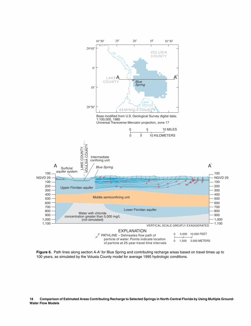
EXPLANATIONPATHLINE – Delineates flow path of

particle of water. Points indicate locationof particle at 25-year travel time intervals

10,000 FEET0

0 3,000 METERS

600

400500

300200

700800900

1,0001,100

100

100

Middle semiconfining unit

Upper Floridan aquifer

Lower Floridan aquiferWater with chloride

concentration greater than 5,000 mg/L(not simulated)

600

400500

300200

7008009001,0001,100

100

100

5,000

1,500

A A

NGVD 29 NGVD 29

Surficialaquifer system

Intermediateconfining unit

Blue SpringLAK

E C

OU

NT

YV

OU

LSIA

CO

UN

TY

VERTICAL SCALE GREATLY EXAGGERATED

ALAKECOUNTY

VOLUSIACOUNTY

SEMINOLE COUNTY

BlueSpring

��

��

��

�

��

10 MILES5

0

0

10 KILOMETERS5S

th

i

.oJ

nsR

v er

LakeMonroe

Base modified from U.S. Geological Survey digital data;1:100,000, 1985Universal Transverse Mercator projection, zone 17

Figure 6. Path lines along section A-A' for Blue Spring and contributing recharge areas based on travel times up to 100 years, as simulated by the Volusia County model for average 1995 hydrologic conditions.


EXPLANATIONPATHLINE – Delineates flow path of

particle of water. Points indicate locationof particle at 25-year travel time intervals

Surficialaquifer system

Intermediateconfining unit

Middle semiconfining unit

Upper Floridan aquifer

Lower Floridan aquiferWater with chloride

concentration greater than 5,000 mg/L(not simulated)

600

400500

300200

7008009001,0001,100

100

100NGVD 29

600

400500

300200

700800900

1,0001,100

100

100NGVD 29

10,000 FEET0

0 3,000 METERS

VERTICAL SCALE GREATLY EXAGGERATED

5,000

1,500

A ABlue SpringLAK

E C

OU

NT

YV

OU

LSIA

CO

UN

TY

Base modified from U.S. Geological Survey digital data;1:100,000, 1985Universal Transverse Mercator projection, zone 17

A

10 MILES5

0

0

10 KILOMETERS5

LAKECOUNTY

VOLUSIACOUNTY

SEMINOLE COUNTY

BlueSpring

��

��

��

�

��

S

th

i

.oJ

nsR

v er

LakeMonroe

Figure 7. Path lines along section A-A' for Blue Spring and contributing recharge areas based on travel times up to 500 years, as simulated by the Volusia County model for average 1995 hydrologic conditions.


Pathline analyses (using a backward-tracking procedure) for the VC model also indicated that a rela-tively small amount of flow to Blue Spring comes from the LFA west of the spring. This flow is not depicted in the area contributing recharge delineated using the VC model because (1) particles stopped at the head-dependent flux boundary implying the flow likely originates outside of the model domain to the southwest and (2) all particles had travel times greater than 100 years. Examination of the GIS data depicting areas contributing recharge for all travel times (app. 1) indicates that for travel times greater than 100 years, the areas contributing recharge to Blue Spring delin-eated by the PF and LCONF models extend southwest of the spring into central Lake County, which is out-side the domain of the VC model.

Silver Springs

The areas contributing recharge to Silver Springs range in area from about 450 to 590 mi2 (fig. 8A, B, C). Combining the areas from each model resulted in a composite area contributing recharge to Silver Springs (fig. 8D). The composite area encom-passes about 730 mi2. The composite area indicates that some of the ground water discharging to Silver Springs originates from areas east of the spring. How-ever, most of the area contributing recharge lies west and south of the spring, which is simulated by each model to be an area of generally higher recharge to the UFA than the area east of the spring.

The composite area for Silver Springs includes land-surface areas that were delineated by all three models, any two models, and a single model (fig. 8D). All three models jointly delineated 48 percent of the total composite area. Two models jointly delineated 26 percent of the total composite area, although the two models were not always the same two models. A single model uniquely delineated 26 percent of the total composite area, although the single model was not always the same model. This indicates the models generally agreed rather than disagreed because 74 per-cent of the total composite area was jointly delineated by at least two models. However, the 26 percent uniquely delineated by a single model is valuable information; these additional areas also may be part of the actual area contributing recharge to Silver Springs,

because the results from each of the ground-water flow models used in this study are assumed to be equally feasible. For the LCONF model, the area con-tributing recharge to Silver Springs intersects the model boundary, and in the absence of this boundary, probably would extend farther west.

Particle travel times derived from a backward-tracking analysis were used to estimate the percentage of spring discharge that has traveled to Silver Springs in a given amount of time from the water source (fig. 9). About 80 percent of the total discharge of Silver Springs simulated by the NCF model reaches the spring within 100 years. For the LCONF and PF models, about 85 percent of the total discharge of Silver Springs reaches the spring within 100 years.

It is likely that differences in areas contributing recharge and in travel time are caused by the different hydraulic properties, boundary conditions, and hydro-logic conditions of the calibration period used by each model. The main hydraulic properties determining the areas contributing recharge to UFA springs are the lea-kance of the ICU and the transmissivity of the UFA. Approximately 29, 50, and 51 percent of the areas contributing recharge to Silver Springs delineated by the LCONF, PF, and NCF models, respectively, lie in areas where the UFA is unconfined. As a result, the leakance of the ICU is not as large a factor as it is for the other springs in determining the areas contributing recharge. In unconfined areas, the specified recharge rate is an important parameter. In west Marion County where the UFA is unconfined, recharge rates vary con-siderably among the three models: 10.1 in/yr for the NCF model, generally 10 to 20 in/yr for the PF model, and about 27 in/yr for the LCONF model. For the NCF model, the lower recharge rate in areas where the UFA is unconfined might explain why the area contributing recharge is larger than the others. Leakage rates from the SAS to the UFA are similar among the models, varying from 0 to 30 in/yr for each model. In addition, the transmissivity of the UFA in all cells in the vicinity of Silver Springs is high (greater than 1,000,000 ft2/d in all models), and differences in transmissivities among models could be regarded as negligible, result-ing in similar travel-time graphs.







delineated

delineated

delineated

20 MILES10

0

0

20 KILOMETERS10


��

��

��

��

��

��

SUMTERCOUNTY

MARIONCOUNTY

ALACHUACOUNTY

PUTNAMCOUNTY

SilverSprings

D

LAKECOUNTY

C

LAKECOUNTY

SUMTERCOUNTY

MARIONCOUNTY

ALACHUACOUNTY

PUTNAMCOUNTY

SilverSprings

��

��

��

��

��

��

NCF

B

LAKECOUNTY

SUMTERCOUNTY

MARIONCOUNTY

ALACHUACOUNTY

PUTNAMCOUNTY

��

��

��

��

��

��

SilverSprings

PF

MODELBOUNDARY

MARIONCOUNTY

A

LAKECOUNTY

SUMTERCOUNTY

MARIONCOUNTY

ALACHUACOUNTY

PUTNAMCOUNTY

SilverSprings

��

��

��

��

��

��

LCONF

Figure 8. Areas contributing recharge to Silver Springs based on travel times up to 100 years as simulated by (A) Lake County/Ocala National Forest (LCONF); (B) Peninsular Florida (PF); (C) North-Central Florida (NCF) models for the average hydrologic conditions of the calibration period; and (D) composite area for all three models.


Lake County / Ocala NationalForest Model, 1998Peninsular Florida Model, 1993-94North-Central Florida Model, May 1995

EXPLANATION

1 10 100 1,000 10,000

TIME, IN YEARS

0

25

50

75

100

PE

RC

EN

T O

F S

PR

ING

DIS

CH

AR

GE

RE

AC

HIN

GT

HE

SP

RIN

G B

YT

HE

IND

ICAT

ED

TIM

E

Figure 9. Particle travel time as a percentage of total spring discharge to Silver Springs based on average hydrologic conditions of the calibration period.


Alexander Springs

The areas contributing recharge to Alexander Springs range in area from about 60 to 70 mi2 (figs. 10A, B, C). Combining the areas from each model resulted in a composite area contributing recharge to Alexander Springs (fig. 10D). The com-posite area encompasses about 110 mi2. The compos-ite area indicates that some of the ground water discharging at Alexander Springs originates from areas north and northwest of the spring. However, most of the area contributing recharge lies southwest of the spring because the prevailing direction of ground-water flow in the UFA in this area is from southwest to northeast.

The composite area for Alexander Springs includes land-surface areas that were delineated by all three models, any two models, and a single model (fig. 10D). All three models jointly delineated 22 per-cent of the total composite area. Two models jointly delineated 22 percent of the total composite area, although the two models were not always the same two models. A single model uniquely delineated 56 percent of the total composite area, although the single model was not always the same model. This indicates the models generally disagreed rather than agreed because 44 percent of the total area was jointly delineated by at least two models. Although the major-ity of the composite area was uniquely delineated by just a single model, this is valuable information. These areas also may be part of the actual area contributing recharge to Alexander Springs, because the results from each of the ground-water flow models used in this study are assumed to be equally feasible.

Particle travel times derived from a backward-tracking analysis were used to estimate the percentage of spring discharge that has traveled to Alexander Springs in a given amount of time from the water source (fig. 11). About 45 percent of the total dis-charge of Alexander Springs simulated by the PF model reaches the spring within 100 years. For the NCF and LCONF models, about 75 and 85 percent, respectively, of the total discharge of Alexander Springs reaches the spring within 100 years.

It is likely that differences in areas contributing recharge and in travel time are caused by the different hydraulic properties, boundary conditions, and hydro-logic conditions of the calibration period used by each model. For example, the average values of leakance of the ICU and transmissivity of the UFA for the model cells within the area contributing recharge to Alex-ander Springs delineated by the LCONF model are

greater than the corresponding values for the areas contributing recharge delineated by either the NCF or PF models (table 4). This might explain why the LCONF model has a larger percentage of discharge with travel times less than 100 years than the other models (fig. 11). Also, the average leakance of the ICU for the model cells within the area contributing recharge to Alexander Springs delineated by the LCONF model is greater than the corresponding value for the PF model, which in turn is greater than the average leakance of the ICU for the NCF model (table 4). This might explain why the smallest area contributing recharge was delineated by the LCONF model (58 mi2), whereas the largest area contributing recharge was delineated by the NCF model (69 mi2).

Silver Glen Springs

The areas contributing recharge to Silver Glen Springs range in area from about 40 to 90 mi2 (fig. 12A, B, C). Combining the areas from each model resulted in a composite area contributing recharge to Silver Glen Springs (fig. 12D). The com-posite area encompasses about 120 mi2. The compos-ite area indicates that some of the ground water discharging at Silver Glen Springs originates from areas northwest and southeast of the spring. Most of the area contributing recharge, however, lies southwest of the spring because the prevailing direction of ground-water flow in the UFA in this area is from southwest to northeast.

The composite area for Silver Glen Springs includes land-surface areas that were delineated by all three models, any two models, and a single model (fig. 12D). All three models jointly delineated 21 per-cent of the total composite area of Silver Glen Springs. Two models jointly delineated 26 percent of the total composite area, although the two models were not always the same two models. A single model uniquely delineated 53 percent of the total composite area, although the single model was not always the same model. This indicates the models generally disagreed rather than agreed when delineating this area because 47 percent of the total area was jointly delineated by at least two models. Although the majority of the com-posite area was uniquely delineated by just a single model, this is valuable information. These areas also may be part of the actual area contributing recharge to Silver Glen Springs, because the results from each of the ground-water flow models used in this study are assumed to be equally feasible.







delineated

delineated

delineated

10 MILES5

0

0

10 KILOMETERS5


D

MARIONCOUNTY

LAKECOUNTY

VO

LU

SIA

AlexanderSprings

��

AlexanderSprings

MARIONCOUNTY

LAKECOUNTY

VO

LU

SIA

C

��

��

��

��

��

VC

��

��

��

��

B

AlexanderSpringsMARION

COUNTY

LAKECOUNTY

VO

LU

SIA

��

��

��

��

��

PF

A

MARIONCOUNTY

LAKECOUNTY

VO

LU

SIA

AlexanderSprings

��

��

��

��

��

LCONF

Figure 10. Areas contributing recharge to Alexander Springs based on travel times up to 100 years as simulated by (A) Lake County/Ocala National Forest (LCONF); (B) Peninsular Florida (PF); (C) North-Central Florida (NCF) models for the average hydrologic conditions of the calibration period; and (D) composite area for all three models.



EXPLANATION

1 10 100 1,000 10,000

TIME, IN YEARS

0

25

50

75

100

PE

RC

EN

T O

F S

PR

ING

DIS

CH

AR

GE

RE

AC

HIN

GT

HE

SP

RIN

G B

YT

HE

IND

ICAT

ED

TIM

E

Figure 11. Particle travel time as a percentage of total spring discharge to Alexander Springs based on average hydrologic conditions of the calibration period.







delineated

delineated

delineated

10 MILES5

0

0

10 KILOMETERS5


D

LAKECOUNTY

VOLUSIACOUNTY

MARIONCOUNTY

PUTNAMCOUNTY

��

��

��

��

��

Silver GlenSprings

LAKECOUNTY

VOLUSIACOUNTY

MARIONCOUNTY

PUTNAMCOUNTY

Silver GlenSprings

C��

��

��

��

��

VC

PF

LAKECOUNTY

VOLUSIACOUNTY

MARIONCOUNTY

PUTNAMCOUNTY

Silver GlenSprings

B��

��

��

��

��

A

LAKECOUNTY

VOLUSIACOUNTY

MARIONCOUNTY

PUTNAMCOUNTY

Silver GlenSprings

��

��

��

��

��

LCONF

Figure 12. Areas contributing recharge to Silver Glen Springs based on travel times up to 100 years as simulated by (A) Lake County/Ocala National Forest (LCONF); (B) Peninsular Florida (PF); (C) North-Central Florida (NCF) models for the average hydrologic conditions of the calibration period; and (D) composite area for all three models.


Particle travel times derived from a backward-tracking analysis were used to estimate the percentage of spring discharge that has traveled to Silver Glen Springs in a given amount of time from the water source (fig. 13). About 45 percent of the total dis-charge to Silver Glen Springs simulated by the PF model reaches the spring within 100 years. For the NCF and LCONF models, about 70 and 85 percent, respectively, of the total discharge of Silver Glen Springs reaches the spring within 100 years.

It is likely that differences in areas contributing recharge and in travel time are caused by the different hydraulic properties, boundary conditions, and hydro-logic conditions of the calibration period used by each model. For example, the area contributing recharge delineated by the PF model is appreciably smaller than

the others, especially toward the southwest. A likely explanation is the magnitude and distribution of leak-age rates to the UFA, which are controlled by the lea-kance of the ICU and the simulated water-level difference between the SAS and UFA. An area of rela-tively high leakage to the UFA (10 to 25 in/yr) is simu-lated by the PF model within the area contributing recharge. Directly southwest is an area of lower lea-kance of the ICU (one-seventh of the leakance to the northeast) and correspondingly low leakage to the UFA (0 to 3 in/yr). This points to a common character-istic of UFA springs—areas contributing recharge gen-erally will be confined as near to, or as far from, the spring as necessary for the spring to capture the amount of recharge to the UFA needed to supply the spring discharge. Another factor that could cause a


EXPLANATION

1 10 100 1,000 10,000

TIME, IN YEARS

0

25

50

75

100

PE

RC

EN

T O

F S

PR

ING

DIS

CH

AR

GE

RE

AC

HIN

GT

HE

SP

RIN

G B

YT

HE

IND

ICAT

ED

TIM

E

Figure 13. Particle travel time as a percentage of total spring discharge to Silver Glen Springs based on average hydrologic conditions of the calibration period.


smaller or larger area contributing recharge is the effects of different hydrologic conditions of the cali-bration period used by each model. Spring discharge simulated by the NCF and LCONF models was 11 and 29 percent, respectively, greater than the 79 ft3/s simu-lated by the PF model (table 2). This might explain, in part, why the areas contributing recharge to Silver Glen Springs delineated by the NCF and LCONF models were about 100 and 50 percent, respectively, larger than the area delineated by the PF model.

Effects of Projected 2020 Ground-Water Withdrawals

The effects of increased ground-water with-drawals estimated to occur in 2020 are of concern because some spring discharge may be captured by supply wells that provide drinking water for Florida’s growing population. This would result in a reduction of the areas contributing recharge to each spring and a corresponding decrease in spring flow. A reduction in spring flow could have an adverse impact on, for example, the ecosystem supported by the spring or recreational activities at the spring.

Areas contributing recharge to springs delin-eated by each model for projected 2020 ground-water withdrawals were about the same size as, or slightly smaller than, the same areas for calibrated model con-ditions. When spring discharge decreases due to increased ground-water withdrawals, the area contrib-uting recharge also decreases, assuming the recharge rate is relatively unchanged. The largest decrease occurred for Blue Spring, where the area contributing recharge delineated by the PF model was reduced about 7 percent. Composite areas contributing recharge to springs for projected 2020 ground-water withdrawals were about the same size as the same areas for calibrated model conditions. The small decreases in areas contributing recharge to the springs is to be expected because of the small reduction in springflow simulated for 2020 conditions (table 2). Because of these small changes, the areas contributing recharge to springs for 2020 conditions are not shown in this report. However, the reader is referred to the GIS databases included in appendix 1 to identify the areas contributing recharge for 2020 conditions.

Limitations

The interpretations from this study have limita-tions. Limiting factors can be broadly categorized into simplifications necessary to simulate the hydrogeo-logic system and assumptions about ground-water flow and particle transport. The reliability of the delin-eation of areas contributing recharge to springs depends on the degree to which the model assump-tions and simplifications represent the natural system. Localized studies of the hydrogeology in the vicinities of individual springs could provide models that better represent the natural system, thus producing more reliable delineations of areas contributing recharge.

All the models assume that ground-water move-ment can be represented with a porous media flow model. This may be a poor assumption because the study area is a covered karst terrain; therefore, conduit and fracture flow probably occur. Fracture and conduit flow may be important because fractures and conduits could cause ground water to take a different path and reach the spring in a shorter amount of time, as opposed to the path and travel time that would result in a porous media (White and White, 2001).

Simplifications are made when discretizing ground-water flow models in space and time. The resolution of the grid spacing limits the detail with which the contributing areas can be delineated. For example, the areas contributing recharge to weak sinks in the flow models are not delineated in the present simulations. Another spatial assumption is that the horizontal hydraulic properties of the aquifer are iso-tropic. This generally is not the case in a karst aquifer system. An important time-related assumption was that the ground-water flow system was at steady state. However, areas contributing recharge to features dis-charging ground water are dynamic. As the stresses applied to natural systems change, the areas contribut-ing recharge change (Masterson and others, 2002). Thus, the applicability of the delineated areas contrib-uting recharge for other time periods depends on the similarity of the assumed steady-state stresses with stresses that occur during those other time periods.

Assumptions also are made when assigning aquifer properties and boundary conditions to the model grid because field data are sparse and natural systems are complex. Therefore, many different inter-pretations of aquifer properties and boundary condi-tions are equally feasible. Hydraulic-head and flow observations used for calibration help constrain the set of feasible aquifer properties and boundary conditions.


However, as a result of sparse data, natural complex-ity, and parameter correlation, a unique set of aquifer properties and boundary conditions that perfectly describe the natural field condition is unattainable. This study addresses this limitation by using four calibrated models, each assumed to represent the flow system equally well.

Finally, caution should be exercised when using areas contributing recharge to springs to address con-cerns about degrading spring water quality. Particle-tracking techniques can only simulate the advective transport of contaminants and cannot be used to calcu-late contaminant concentrations in ground water because these techniques do not consider dispersion, diffusion, degradation, or retardation processes. It is feasible for a source of contamination external to the areas contributing recharge to springs to adversely affect the springs’ water quality. This could happen if a contaminant moves by dispersion and/or diffusion into the areas contributing recharge to springs. The geochemistry of a contaminant also affects its impact on the springs water quality.

Despite these limitations, the composite areas contributing recharge to springs may be the best estimates available because they were derived from four ground-water flow models that each account for natural heterogeneities. Each model is an alternative way of representing the ground-water system. In com-plex, natural systems, selecting only one model as superior to all others often is difficult, especially where only a limited amount of data describing the system is available. It may be necessary to accept with equal confidence the range of results provided by the various models.

SUMMARY

Springs are an important water resource to be protected by the State of Florida, particularly in parts of north-central Florida where many of the State’s most productive springs occur. Springs contribute freshwater to sensitive ecosystems where many biological communities reside, provide a resource for recreational activities, and contribute to local econo-mies. Considering the importance of springs, the Florida Department of Environmental Protection wants to define the areas contributing recharge to springs for regulatory and planning purposes. In the past, these areas often were delineated based on potentiometric-surface maps. Ground-water flow models allow a more detailed delineation.

Areas contributing recharge to springs are defined in this report as the land-surface areas wherein water entering the ground-water system at the water table eventually discharges to a spring. Particle track-ing was performed to delineate these areas for Blue Spring, Silver Springs, Alexander Springs, and Silver Glen Springs by using four ground-water flow models. The four models are the Peninsular Florida (PF) model (Sepúlveda, 2002), the Lake County/Ocala National Forest (LCONF) model (Knowles and others, 2002), the North-Central Florida (NCF) model (Motz and Dogan, 2002), and the Volusia County (VC) model (S.A. Williams, written commun., St. Johns River Water Management District, 2003). Calibrated model conditions and projected 2020 ground-water with-drawals were used to delineate the areas contributing recharge to each spring.

As expected, different models predicted differ-ent areas contributing recharge to each spring. Possi-ble explanations for the differences are (1) different ground-water levels and flows resulting from the dif-ferent hydrologic conditions, such as ground-water withdrawals and rainfall variations, during the time periods used to calibrate each model; (2) different val-ues and distributions of hydraulic properties for each of the four models, all of which are considered to be equally feasible because each model matched its respective calibration data reasonably well; and (3) different boundary conditions among models.

Combining areas contributing recharge from all models produced a composite area for each spring. For Blue Spring, the composite area covers about 130 square miles (mi2), 54 percent of which was jointly delineated by two or three models. Most of the source water for Blue Spring originates from areas east of the St. Johns River. However, some of the source water originates from areas west of the St. Johns River, even though the spring is east of the river. The composite area for Silver Springs encompasses about 730 mi2, 74 percent of which was jointly delineated by two or three models. Most of the source water originates from areas west and south of Silver Springs. For Alexander Springs, the composite area covers about 110 mi2, 44 percent of which was jointly delineated by two or three models. Most of the source water originates from areas southwest of Alexander Springs. For Silver Glen Springs, the composite area covers about 120 mi2, 47 percent of which was jointly delineated by two or three models. Most of the source water originates from areas southwest of Silver Glen Springs.

Summary 29

Areas contributing recharge to springs delin-eated by each model for projected 2020 ground-water withdrawals were about the same size as, or slightly smaller than, the same areas for calibrated model con-ditions. The largest decrease occurred for Blue Spring, where the area contributing recharge delineated by the PF model was reduced about 7 percent. Composite areas contributing recharge to springs for projected 2020 ground-water withdrawals were about the same size as the same areas for calibrated model conditions.

Several limitations were apparent in the use of multiple ground-water flow models to delineate com-posite areas contributing recharge. These limitations can be broadly categorized into model simplifications and assumptions regarding ground-water flow and particle transport. The reliability of composite area delineations depends on the degree to which model simplifications and assumptions represent the natural system. Despite the limitations, these composite areas contributing recharge to springs may be the best esti-mates available because the composite areas were derived from four ground-water flow models that each account for natural heterogeneities.

REFERENCES

Barlow, P.M., 1994a, Particle-tracking analysis of contributing areas of public–supply wells in simple and complex flow systems, Cape Cod, Massachusetts: U.S. Geological Survey Water Supply Paper 2434, 66 p.

———1994b, Two- and three-dimensional pathline analy-sis of contributing areas to public-supply wells of Cape Cod, Massachusetts: Ground Water, v. 32, no. 3, p. 399-410.

Camp Dresser and McKee, Inc., 1984, Design development report for southwest Orange County regional wastewater treatment facilities water conservation project: for the Board of County Commissioners, Orange County, Fla., technical report and two appendices.

Harbaugh, A.W., and McDonald, M.G., 1996, User’s documentation for MODFLOW-96, an update to the U.S. Geological Survey modular finite-difference ground-water flow model: U.S. Geological Survey Open-File Report 96-485, 56 p.

Harbaugh, A.W., Banta, E.R., Hill, M.C., and McDonald, M.G., 2000, MODFLOW-2000, the U.S. Geological Survey modular ground water model—User guide to modularization concepts and the ground water flow process: U.S. Geological Survey Open-File Report 00-92, 121 p.

Hill, M.C., Banta, E.R., Harbaugh, A.W., and Anderman, E.R., 2000, MODFLOW-2000, the U.S. Geological Survey modular ground water model—User guide to the observation, sensitivity, and parameter estimation processes and three post processing programs: U.S. Geological Survey Open-File Report 00-184, 209 p.

Knochenmus, D.D., and Hughes, G.H., 1976, Hydrology of Lake County, Florida: U.S. Geological Survey Water-Resources Investigations, 76-72, 100 p.

Knochenmus, L.A., and Robinson, J.L., 1996, Descriptions of anisotropy and heterogeneity and their effect on ground-water flow and areas of contribution to public supply wells in a karst carbonate aquifer system: U.S. Geological Survey Water-Supply Paper 2475, 47 p.

Knowles, L., Jr., 1996, Estimation of evapotranspiration in the Rainbow Springs and Silver Springs Basins in north-central Florida: U.S. Geological Survey Water-Resources Investigations Report 96-4024, 37 p.

Knowles, L., Jr., O’Reilly, A.M., and Adamski, J.C., 2002, Hydrogeology and simulated effects of ground-water withdrawals from the Floridan aquifer system in Lake County and in the Ocala National Forest and vicinity, north-central Florida: U.S. Geological Survey Water-Resources Investigations Report 02-4207, 140 p.

Kohout, F.A., 1960, Cyclic flow of salt water in the biscayne aquifer of southeastern Florida: Journal of Geophysical Research, v. 65, no. 7, p. 2,133-2,141.

Masterson, J.P., and Walter, D.A., 2000, Delineation of ground-water recharge areas, western Cape Cod, Massachusetts: U.S. Geological Survey Water-Resources Investigations Report 00-4000, 1 pl.

Masterson, J.P., Hess, K.M., Walter, D.A., and LeBlanc, D.R., 2002, Simulated changes in the sources of ground water for public supply wells, ponds, streams, and coastal areas on western Cape Cod, Massachusetts: U.S. Geological Survey Water-Resources Investiga-tions Report 02-4143, 12 p.

McDonald, M.G., and Harbaugh, A.W., 1988, A modular three-dimensional finite-difference ground-water flow model: U.S. Geological Survey Techniques of Water Resources Investigations, book 6, chap. A1, 586 p.

Motz, L.H., and Dogan, A., 2002, Revised north central Florida regional groundwater flow model: A report prepared for the St. Johns River Water Management District, 107 p.

Murray, L.C., Jr., and Halford, K.J., 1996, Hydrogeologic conditions and simulations of ground-water flow in the Greater Orlando Metropolitan Area, east-central Florida: U.S. Geological Survey Water-Resources Investigations Report 96-4181, 100 p.

Phelps, G.G., 1994, Hydrogeology, water quality, and potential for contamination of the Upper Floridan aquifer in the Silver Springs ground-water basin, central Marion County, Florida: U.S. Geological


Survey Water-Resources Investigations Report 92-4159, 69 p., 5 pl.

Pollock, D.W., 1989, Documentation of computer programs to compute and display pathlines using results from the U.S. Geological Survey modular three-dimensional finite-difference ground-water flow model: U.S. Geological Survey Open-File Report 89-381, 188 p.

———1994, User’s guide for MODPATH/MODPATH-PLOT, version 3, a particle tracking post processing package for MODFLOW, the U.S. Geological Survey finite-difference ground-water flow model: U.S. Geo-logical Survey Water-Resources Investigations Report 98-4080.

Reilly, T.E., 2001, System and boundary conceptualization in ground-water flow simulation: U.S. Geological Survey Techniques of Water-Resources Investigations, book 3, chap. B8, 30 p.

Reilly, T.E., and Pollock, D.W., 1993, Factors affecting areas contributing recharge to wells in shallow aquifers: U.S. Geological Survey Water-Supply Paper 2412, 21 p.

Renken, R.A., Patterson, R.D., Orzol, L.L., and Dixon, J., 2001, Approach for delineation of contributing areas and zones of transport to selected public-supply wells using a regional ground-water flow model, Palm Beach County, Florida: U.S. Geological Survey Water-Resources Investigations Report 01-4158, 56 p.

Robinson, J.L., 1995, Hydrogeology and results of tracer tests at the old Tampa well field in Hillsborough County, with implications for wellhead-protection strategies in west-central Florida: U.S. Geological Survey Water-Resources Investigations Report 93-4171, 63 p.

Rosenau, J.C., Faulkner, G.L., Hendry, C.W., Jr., and Hull, R.W., 1977, Springs of Florida: Florida Bureau of Geology Bulletin No. 31 (revised), 461 p.

Sepúlveda, N., 2002, Simulation of ground-water flow in the intermediate and Floridan aquifer systems in peninsular Florida: U.S. Geological Survey Water-Resources Investigations Report 02-4009, 130 p.

Sumner, D.M., 2001, Evapotranspiration from a cypress and pine forest subjected to natural fires, Volusia County, Florida, 1998-99: U.S. Geological Survey Water-Resources Investigation Report 01-4245, 56 p.

Sumner, D.M., and Bradner, L.A., 1996, Hydraulic characteristics and nutrient transport and transformation beneath a rapid infiltration basin, Reedy Creek Improvement District, Orange County, Florida: U.S. Geological Survey Water-Resources Investigations Report 95-4281, 51 p.

White, W.B., and White, E.L., 2001, Conduit fragmentation, cave patterns, and the localization of karst ground water basins: The Appalachians as a test case: Theoretical and Applied Karstology, v. 13–14, p. 9-23.

References 31

comparison of estimated areas contributing recharge to ... · spring using ground-water withdrawals...

Documents