comparison of dijkstra's algorithm with other proposed ...iaiest.com/dl/journals/7- iaj of...

International Academic

Journal of

Science

and

Engineering International Academic Journal of Science and Engineering Vol. 3, No. 7, 2016, pp. 53-66.

ISSN 2454-390X www.iaiest.com

53

International Academic Institute for Science and Technology

Comparison of Dijkstra's Algorithm with other proposed

algorithms

Zafar Ali Department of Computer Sciene, Virtual University of Pakistan

Abstract

In 1959, Dijkstra proposed an algorithm to determine the shortest path between two nodes in a graph. The

algorithm gets lots of attention as it can solve many real life problems. The algorithm is a greedy type

algorithm. Other types of algorithms are also developed and compared. Application based improvements

are done on the original algorithm. Time complexity of the algorithm is improved at the cost of space

complexity. Implementation of such algorithm is possible as modern hardware allows more space

complexity.

Keywords: Dijkstra‘s algorithm, shortest path, graph, node, edge, time complexity, space complexity.

Abreviations:

1. Dijkstra‘s Algorithm (DA).

2. Shortest Path (SP).

Introduction

Dijkstra‘s Algorithm (DA) gets a wide attention as it solves an important problem of graph theory, of

finding out the ―Shortest Path (SP)‖. For a graph with each edge having a weight or path length the

algorithm determines the SP between two selected vertices. The algorithm can be best understood through

an example. Following figure shows a specific graph.

International Academic Journal of Science and Engineering,

Vol. 3, No. 7, pp. 53-66.

54

Figure 1(a) An example graph. (b) Execution steps of Dijkstra's Algorithm [1].

The problem is to determine the SP from node d to node j. The top most row in the table in fig. 1b shows

the number of iterations. For init or 0th

iteration all the distances from source d to nodes other than d are

taken as infinity. Here the symbol ∞ stands for ‗unknown‘. In computation a very large number is put in

place of infinity to refuse the unknown. Path length between nodes d to d is obviously zero. These values

are given in the first column of the table.

In the 1st iteration the distances from source to adjacent nodes replace the initial infinite value. In this

case, adjacent nodes are ‗a‘ and ‗h‘. Distance from node d to h is 1 and to a is 4 as shown in the graph of

figure 1. In the 2nd

iteration the active vertex is h as it is with the shortest distance from d. Now the sum

of the distances from d to h and h to adjacent nodes are determined and compared with the direct path if

any. The smaller value is put in the 3rd

column. For example, distance from d to e is obtained as distance

between d to h (1) + distance between h to e (5). So the total distance 6 is put in the 5th

row and the 3rd

column of the table. The distance between active vertex h to a is either the sum of distances d to h (1) and


Vol. 3, No. 7, pp. 53-66.

55

h to a (10) 11 or the direct path distance 4. The smaller value 4 is put in the 1st row and the 1

st column of

the table. Since ‗a‘ becomes the active vertex in the 3rd

iteration due to the direct path from d the active

vertex h in iteration 2 is discarded from the final route. The final route obtained so far is: dae with

path length 6.

The iteration stops when the destination node j is reached as active vertex. Then the final route becomes

da e f i j with SP length 11.

Determination of SP is a real life problem that needs to be solved from time to time and place to place.

This algorithm can be applied directly to find out the shortest distance between two stations [2]. The

graph represents road or rail connection for all the available stations. The algorithm requires

modifications when needs to deal with variable number edges. This arises when some of the roads might

be blocked for repair work or bad weather condition.

The algorithm finds broader applications when path length can represent something else. If a project can

be divided into several alternative tasks then a graph can be constructed with nodes representing the tasks

and the path lengths are replaced by time of execution of tasks. In this case DA determines the

completion of the project in the shortest time. In some cases, application specific modifications are

essential. DA does not work when certain path lengths become negative. Algorithms were proposed to

handle this kind of situation [1].

As technology advances the algorithm finds more applications. The algorithm gets a great attention with

developments of routing strategies in computer and mobile networks.

Though the algorithm was proposed long back [3] lots of innovative ideas are reported off-late for

improvement of the algorithm. To speed up execution, various types of data structures are used.

More memory is allocated to store intermediate results that are reused to eliminate some computation

steps. Thus time complexity is improved at the cost of space complexity. This is a general trend for all

algorithm improvement. As the modern hardware can provide more memory a higher space complexity is

quite feasible.

Another trend is to divide the network into parts and applying the algorithm for the sub-networks. As the

time complexity is dependent on square of number of nodes time complexity is greatly improved for

smaller number of nodes. Further specific networks were reported for which modified DA works more

efficiently and time complexity reduces.

DA is a greedy type algorithm that looks for the best immediate result. Other techniques are also tried and

results are compared.

There are numerous proposed algorithms for SP and the number is growing at a very fast rate. In this

work, some of the selected algorithms that can be applied to SP are compared.


Vol. 3, No. 7, pp. 53-66.

56

Related Work

For real road networks determination of SP from place to place is extremely important. Zhan [4]

compared 15 algorithms for this application. Following table lists all these algorithms.

Table 1: List of 15 algorithms [4].

Abbreviation Implementation

BFM Bellman-Ford-Moore

BFP Bellman-Ford-Moore with Parent -- checking

DKQ Dijikstra‘s Native Implementation

DKB Dijikstra‘s Buckets – Basic Implementation

DKM Dijikstra‘s Buckets – Overflow Bag

DKA Dijikstra‘s Buckets – Approximate

DKD Dijikstra‘s Buckets – Double

DKF Dijikstra‘s Heap – Fibonacci

DKH Dijikstra‘s Heap – k—array

DKR Dijikstra‘s Heap – R—Heap

PAP Graph Growth – Pape

TQQ Graph Growth With Two Queues – Pallottino

THR Threshold Algorithm

GR1 Topological Ordering – Basic

GR2 Topological Ordering -- Distance Updates

All these algorithms were implemented in C language. For one-to-all SP best performance is exhibited by

TQQ algorithm. For one-to one or one-to-some SPs, DA offers some advantages because it can be

terminated as soon as the destination node is reached. Two variations of DA, DKA and DKB were

implemented. DKA works better for path length less than 1500. Above 1500 DKB is better. This is

observed from the implemented algorithms. There is no explanation for such behavior. If DKB needs to

be applied for path length less than 1500 the lengths can be scaled up to make it above 1500. No such

guideline is given in this paper. The worst case complexity of DKA is O(mb+n(b+C/b)). Here n and m

represent number of nodes and edges respectively. b is a chosen constant. A node is not allowed to be

scanned more than b times. C is the maximum path length in a network.Time complexity is improved at

the cost of space complexity. Complexities of TQQ and DKB are not reported in this paper.

Arjun et al. [5] improved DA by using efficient data structure. Here heap sort is used to find the SP. In

heap sort the time complexity is log(n) where n is the number of nodes to be sorted.

Magzhan and Jani [6] analyzed and compared 4 algorithms for SP determination. Following table gives

the time complexities of 3 algorithms.


Vol. 3, No. 7, pp. 53-66.

57

Table 2: Time Complexity**

[6].

Algorithm Time Compexity

Dijkstra n2 + m

Bellman-Ford n3

Floyd-Warshall nm

** nNo. of nodes. mNo. of edges.

Time complexity for the 4th

algorithm, Genetic Algorithm cannot be estimated as it has many random

processes. Only ‗selection‘ is a deterministic process. Time complexity is estimated by other authors. As

it depends on population size of the chromosome complexity cannot be compared with the other 3

algorithms given in the above table.

Betz and Rose [7] determined SP for routing of components in an FPGA. They developed a tool named

VPR that can do initial placement and routing of components in an FPGA. Routing is done using

―Pathfinder Negotiated Congestion Algorithm‖. In this algorithm, SP for nets with small number of nodes

is determined by DA. Then global routing is done with a modified version. Time complexity is greatly

improved as the algorithm works for small number of nodes for each net.

Figure 2: Routing tracks decided by various tools. Placement is done by Altor [7].

Result shows VPR requires minimum tracks for all benchmarked blocks.


Vol. 3, No. 7, pp. 53-66.

58

Huang et al. [8] improved DA by allowing more space complexity. Following figure gives the flowchart

of their algorithm.

Figure 3: Flowchart of the developed algorithm [8].


Vol. 3, No. 7, pp. 53-66.

59

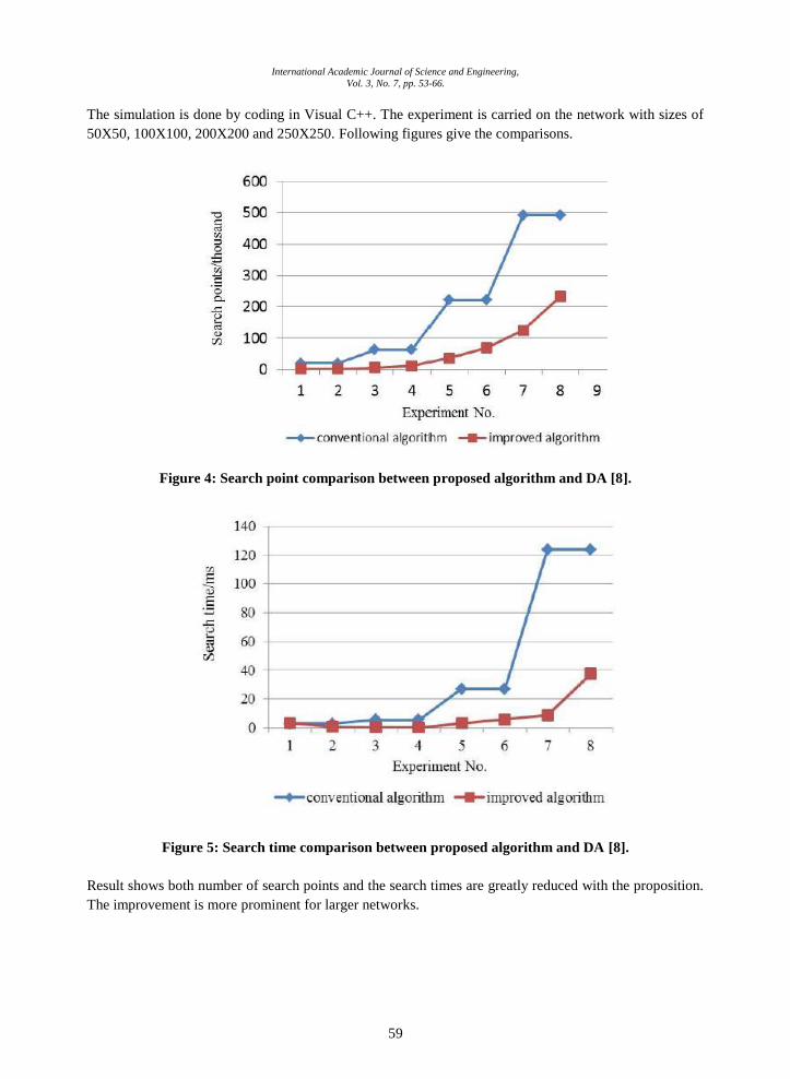
The simulation is done by coding in Visual C++. The experiment is carried on the network with sizes of

50X50, 100X100, 200X200 and 250X250. Following figures give the comparisons.

Figure 4: Search point comparison between proposed algorithm and DA [8].

Figure 5: Search time comparison between proposed algorithm and DA [8].

Result shows both number of search points and the search times are greatly reduced with the proposition.

The improvement is more prominent for larger networks.


Vol. 3, No. 7, pp. 53-66.

60

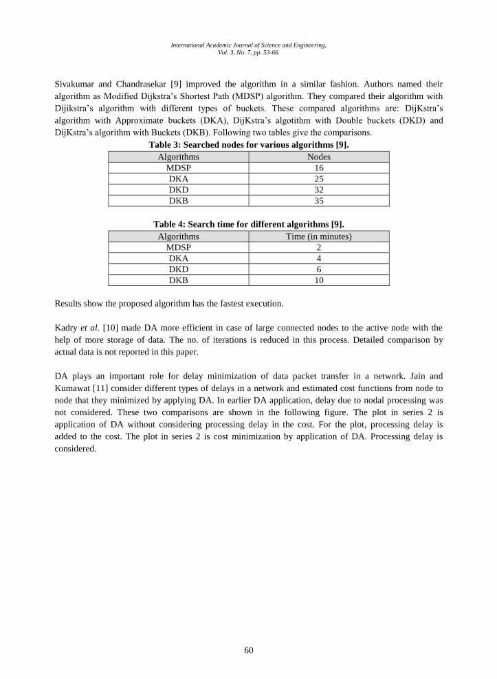
Sivakumar and Chandrasekar [9] improved the algorithm in a similar fashion. Authors named their

algorithm as Modified Dijkstra‘s Shortest Path (MDSP) algorithm. They compared their algorithm with

Dijikstra‘s algorithm with different types of buckets. These compared algorithms are: DijKstra‘s

algorithm with Approximate buckets (DKA), DijKstra‘s algotithm with Double buckets (DKD) and

DijKstra‘s algorithm with Buckets (DKB). Following two tables give the comparisons.

Table 3: Searched nodes for various algorithms [9].

Algorithms Nodes

MDSP 16

DKA 25

DKD 32

DKB 35

Table 4: Search time for different algorithms [9].

Algorithms Time (in minutes)

MDSP 2

DKA 4

DKD 6

DKB 10

Results show the proposed algorithm has the fastest execution.

Kadry et al. [10] made DA more efficient in case of large connected nodes to the active node with the

help of more storage of data. The no. of iterations is reduced in this process. Detailed comparison by

actual data is not reported in this paper.

DA plays an important role for delay minimization of data packet transfer in a network. Jain and

Kumawat [11] consider different types of delays in a network and estimated cost functions from node to

node that they minimized by applying DA. In earlier DA application, delay due to nodal processing was

not considered. These two comparisons are shown in the following figure. The plot in series 2 is

application of DA without considering processing delay in the cost. For the plot, processing delay is

added to the cost. The plot in series 2 is cost minimization by application of DA. Processing delay is

considered.


Vol. 3, No. 7, pp. 53-66.

61

Figure 6: Comparison of cost functions with and without considering delay due to nodal processing

[11].

Result shows cost optimization improves after consideration of additional delay.

Singal and Chhillar [12] used Global Positioning System (GPS) to find the initial node. Then DA is

applied to find the destination node by the SP. Following figure gives the flowchart of their algorithm.


Vol. 3, No. 7, pp. 53-66.

62

Figure 7: Flowchart of the proposed algorithm [12].


Vol. 3, No. 7, pp. 53-66.

63

This flow is applied for the graph given in the following figure. Following table gives the resultant nodes

in every step.

Figure 8: Graph considered for the proposed algorithm [12].

Table 5: Resultant nodes in every step [12].

Steps N Position Dist-

ance

D(B),

Path

D(C),

Path

D(D),

Path

D(E),

Path

D(F), Path

1 {A} (2,3) 0 3,A-B 5,A-C ∞,- ∞,- ∞,-

2 {A,B} (5,7) 5 3,A-B 4,A-B-C 5,A-B-D 4,A-B-E ∞,-

3 {A,B,C} (8,11) 10 3,A-B 4,A-B-C 5,A-B-D 4,A-B-E ∞,-

4 { A,B,C,D} (11,15) 15 3,A-B 4,A-B-C 5,A-B-D 4,A-B-E 7,A-B-E-F

5 { A,B,C,D,E} (14,19) 20 3,A-B 4,A-B-C 5,A-B-D 4,A-B-E 7,A-B-E-F

6 { A,B,C,D,E,F} (17,23) 25 3,A-B 4,A-B-C 5,A-B-D 4,A-B-E 7,A-B-E-F

Sniedovich [13] gave some idea to link dynamic programming with DA. This will generate more

attention from Operations Research and Management Science.

Orlin et al. [14] proposed efficient algorithm for special configuration of the graph. When there are a few

distinct edges the algorithm works very efficiently. If there are n vertices, m edges and K distinct edge

lengths time complexity can be given by O(m) if nK≤2m and O(mlog(nK/m)) otherwise.

Analysis

Dijkstra‘s algorithm gets lots of attention as it can solve many real life problems.

More general algorithms are proposed to take care of negative and irrational edge lengths.

For some applications e.g. shortest distance between two cities connected by roads it seems, DA can

be applied directly. In this case also modification of DA is needed. For safety, a road might be

blocked for bad weather condition. Rest of the road work remains the same. DA must work for a part

of the graph.

With the use of GPS the initial node can be found out. A modified algorithm is needed for inclusion

of initial node and calculation of Euclidean distances.


Vol. 3, No. 7, pp. 53-66.

64

Improvement might be effective for a particular configuration. The modification that can be done for

a graph with too many edges is quite different for a graph with a small no. of edges of different

lengths.

A large network can be divided into smaller congested networks. A detailed routing for smaller

networks and subsequent global routing for the whole network proves to be very efficient for FPGA.

For routing of data packets in a network DA can be used. Here time lapse for data transfer from node

to node should be considered in place of distance. All possible delays must be considered and

modeled to give the effective delay or cost function. This cost should be minimized. The problem

demands attention of researchers as the delay varies with channel condition and transmission of other

data packets.

Time complexity of the algorithm can be reduced at the cost of increasing space complexity.

Intermediate results are stored to avoid repeated computation that increases space complexity. As

modern hardware provide more memories the space complexity remains feasible though it is large.

Following table gives the features of some of the selected algorithms for shortest path determination.

Time complexities, if available, are compared.

Algorithm /

Inventor‘s

Name

Special Features Time Complexity Source of

Information

Dijkstra‘s

Algorithm

Finds out the shortest path

between any two nodes in a

graph.

n2 + m = O(n

2) [1, 6].

L. Ford Edge length can be

negative.

O(nm) [1]

Gallo and

Pallottino

Edge length can be

irrational.

O(2n) [1]

DKA With more space

complexity a reduction in

time complexity

O(mb+n(b+C/b)) [4]

Arjun et al. For networks with large

number of edges.

log(n) for heap sort.

n2 + log(n) in total.

[5]

Bellman-

Ford

Networks with small

number of nodes

n3

[6]

Floyd-

Warshall

Networks with small

number of edges

nm [6]


Vol. 3, No. 7, pp. 53-66.

65

Genetic

Algorithm

For large networks. Correct

result can have a high

probability. But the

probability is always less

than 1.

Cannot be determined for

random processes. It can be

given only for the process

―Selection‖. But it is related

to population size. It has no

direct relation with network

parameters.

[6]

Pathfinder

Negotiated

Congestion

Algorithm

For detailed routing in a

congested network with

small number of nodes. A

network with small n and

comparable m.

Not reported [7]

Orlin et al. For special network with

small number of distinct

edges.

O(m) if nK≤2m and

O(mlog(nK/m)) otherwise.

[14]

** n No. of nodes.

m No. of edges.

b A chosen constant. Each node can be touched b times at most.

CThe largest path length in a network. It should be an integer.

K No. of distinct edges.

Conclusion

Some selected algorithms are compared with Dijkstra‘s algorithm. Time complexities if available are

compared. Reported simulation times are compared. Application based improvements are analyzed.

With the advancement of technology the algorithm will get more applications. Focused research is needed

for application based improvement in the algorithm. Time complexity will be improved at the cost of

space complexity as better hardware with more storage space will emerge.

References

[1] A. Drozdek, Data Structures and Algorithms in Java, 2nd

ed,. Cengage Learning, US, 2010, pp. 383 - 393.

[2] A. Jain, U. Datta, and N. Joshi, ―Implemented modification in Dijkstra‘s Algorithm to find the shortest

path for N nodes with constraint‖, International Journal of Scientific Engineering and Applied Science,

vol. 2, no. 2, pp. 420 – 426, February 2016.

[3] E.W Dijkstra,., ―A note on two problems in connection with graphs‖, Numerische Mathematik, vol. 1 ,

pp. 269–271, 1959.

[4] F.B. Zhan, ―Three fastest shortest path algorithms on real road networks: data structures and procedures‖,

Journal of Geographic Information and Decision Analysis, vol.1, no. 1, pp. 70 – 82, 1997.

[5] R.K. Arjun, P. Reddy, Shama, and M. Yamuna, ―Research on the optimization of Dijkstra‘s algorithm

and its applications‖, International Journal of Science Technology and Management, vol. 4, no. 1, pp. 304

– 309, April 2015.


Vol. 3, No. 7, pp. 53-66.

66

[6] K. Magzhan and H.M. Jani, ―A review and evaluations of shortest path algorithms‖, International Journal

of Scientific and Technology Research, vol. 2, no. 6, pp. 99 -104, June 2013.

[7] V. Betz and J. Rose, ―VPR: A new packing, placement and routing tool for FPGA research‖, in Proc. 7th

International Workshop on Field Programmable Logic and Applications, , London, UK, Sept 1 – 3, 1997,

pp. 213 – 222.

[8] Y. Huang, Q. Yi, and M. Shi, ―An improved Dijkstra shortest path algorithm‖, in Proc. 2nd

International

Conference on Computer science and Electronics Engineering, Atlantis Press, Paris, France, 2013, pp.

226 – 229.

[9] S. Sivakumar and C. Chandrasekar, ―Modified Dijkstra‘s shortest path algorithm‖, International Journal

of Innovative Research in Computer and Communication Engineering, vol. 2, no. 11, pp. 6450 – 6456,

November 2014.

[10] S. Kadry, A. Abdallah, and C. Joumaa, ―On the optimization of Dijkstra‘s algorithm‖, D. Yang (Ed.),

Informatics in Control, Automation and Robotics, vol. 2, vol. 133 of the series lecture notes in Electrical

Engineering, pp. 393 – 397, Springer-Verlag, Berlin Heidelberg, 2011.

[11] C. Jain and J. Kumawat, ―Processing delay consideration in Dijikstra‘s algorithm‖, International Journal

of Advanced Research in Computer Science and Software Engineering, vol. 3, no. 8, pp. 407 – 411,

August 2013.

[12] P. Singal and R.S, Chhillar, :‖ Dijikstra shortest path algorithm using global positioning system‖,

International Journal of Computer Applications, vol. 101, no. 6, pp. 12 – 18, September 2014.

[13] M. Sniedovich, ―Dijkstra‘s algorithm revisited: the dynamic programming connexion‖, Control and

Cybernatics, vol. 35, no. 3, pp. 599 – 620, 2006.

J.B. Orlin, K. Madduri, K. Subramani, and M. Williamson, ―A faster algorithm for the single source shortest

path problem with few distinct positive lengths‖, Journal of Discrete Algorithms, vol. 8, no. 2, pp. 189 –

198, June 2010.

comparison of dijkstra's algorithm with other proposed ...iaiest.com/dl/journals/7- iaj of...

Documents