comparison of ansys elements shell181 and solsh190 · ansys shell elements contact:...
TRANSCRIPT

Comparison of ANSYS elementsSHELL181 and SOLSH190
Biswajit Banerjee[1]
Jeremy Chen, Raj Das, Anjukan Kathirgamanathan[2]
2011-July-13
[1] [email protected], Industrial Research Limited, NZ[2] Department of Mechanical Engineering, University of Auckland, NZ
AnsysShellCompare.pdf Page 1 of 53

ANSYS shell elementsContact: [email protected] 2011-July-13
Contents
Abstract 3
1 Introduction 3
2 Simply supported isotropic plate under uniform load 4
2.1 Exact solutions . . . . . . . . . . . . . . . . . . . . . . . . . . . . . . . . . . . . . . . . . . . . . 4
2.2 The SHELL181 element . . . . . . . . . . . . . . . . . . . . . . . . . . . . . . . . . . . . . . . 6
2.3 The SOLSH190 element . . . . . . . . . . . . . . . . . . . . . . . . . . . . . . . . . . . . . . . 7
2.4 The SOLID185 element . . . . . . . . . . . . . . . . . . . . . . . . . . . . . . . . . . . . . . . 10
3 Isotropic plate loaded by boundary moments 16
3.1 Exact solutions . . . . . . . . . . . . . . . . . . . . . . . . . . . . . . . . . . . . . . . . . . . . . 16
3.2 SHELL181 element . . . . . . . . . . . . . . . . . . . . . . . . . . . . . . . . . . . . . . . . . . 17
3.3 SOLSH190 element . . . . . . . . . . . . . . . . . . . . . . . . . . . . . . . . . . . . . . . . . . 17
4 Isotropic cantilever plate with concentrated edge load 21
4.1 Exact solution . . . . . . . . . . . . . . . . . . . . . . . . . . . . . . . . . . . . . . . . . . . . . . 21
4.2 SHELL181 element . . . . . . . . . . . . . . . . . . . . . . . . . . . . . . . . . . . . . . . . . . 22
4.3 SOLSH190 element . . . . . . . . . . . . . . . . . . . . . . . . . . . . . . . . . . . . . . . . . . 22
4.4 SOLID185 element . . . . . . . . . . . . . . . . . . . . . . . . . . . . . . . . . . . . . . . . . . 24
5 Cantilever orthotropic plate with concentrated edge load 27
5.1 SHELL181 element . . . . . . . . . . . . . . . . . . . . . . . . . . . . . . . . . . . . . . . . . . 27
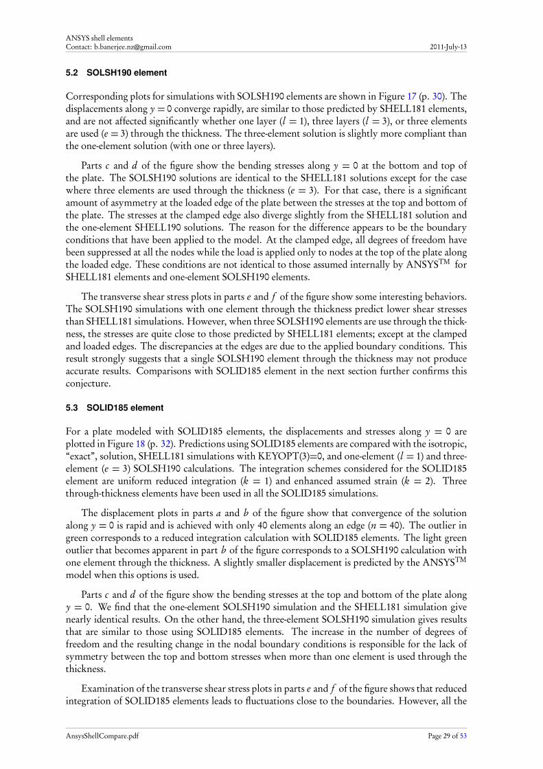
5.2 SOLSH190 element . . . . . . . . . . . . . . . . . . . . . . . . . . . . . . . . . . . . . . . . . . 29
5.3 SOLID185 element . . . . . . . . . . . . . . . . . . . . . . . . . . . . . . . . . . . . . . . . . . 29
6 Cantilevered isotropic sandwich plate with concentrated edge load 33
6.1 Exact solution . . . . . . . . . . . . . . . . . . . . . . . . . . . . . . . . . . . . . . . . . . . . . . 33
6.2 SHELL181 element . . . . . . . . . . . . . . . . . . . . . . . . . . . . . . . . . . . . . . . . . . 35
6.3 SOLSH190 element . . . . . . . . . . . . . . . . . . . . . . . . . . . . . . . . . . . . . . . . . . 40
6.4 SOLID185 element . . . . . . . . . . . . . . . . . . . . . . . . . . . . . . . . . . . . . . . . . . 42
7 Cantilevered anisotropic sandwich plate with concentrated edge load 45
7.1 SHELL181 element . . . . . . . . . . . . . . . . . . . . . . . . . . . . . . . . . . . . . . . . . . 46
7.2 SOLSH190 element . . . . . . . . . . . . . . . . . . . . . . . . . . . . . . . . . . . . . . . . . . 46
7.3 Wall attachment . . . . . . . . . . . . . . . . . . . . . . . . . . . . . . . . . . . . . . . . . . . . . 46
8 Cantilevered anisotropic sandwich plate under acceleration load 50
9 Summary 52
AnsysShellCompare.pdf Page 2 of 53
ANSYS shell elementsContact: [email protected] 2011-July-13
Abstract
Plate and shell elements are indispensable for the study of the mechanics of complex structures. Two classesof shell elements are commonly used in finite element analyses of thin structures, classical two-dimensionalelements and three-dimensional continuum elements. Users of commercial finite element software, such asANSYSTM , are often unsure of the relative strengths and weaknesses of these elements and of the appro-priate use of these elements. This report provides data that can be used as a basis for the selection of shellelements for engineering analysis and design. The displacements and stresses predicted by two ANSYSTM
shell elements, SHELL181 and SOLSH190, are compared with exact solutions and full three-dimensionalsimulations for several geometries and boundary conditions. We conclude that classical shell, SHELL181,elements and solid shell, SOLSH190, elements behave in a similar, though not identical, manner for manysituations. For instance, SHELL181 elements generate poor solutions compared to SOLSH190 elements forsandwich plates with isotropic layers and small core to facesheet stiffness ratios. However, for low stiffnesscores of moderately high shear stiffness, both SHELL181 and SOLSH190 elements perform adequately. Wealso note that plates modeled with a single layer of SOLSH190 elements are extremely stiff in bending andwe recommend at least three elements through the plate thickness for reasonable results. Also, boundaryconditions have to be applied to all the nodes of SOLSH190 elements to achieve the correct mid-surface de-formation behavior. The solid shell element provided by ANSYSTM can be used to replace standard shellelements provided care is taken during its use.
1 Introduction
A search of the web pages that discuss finite element software packages often brings up the issue ofusing “solid shell” elements. Questions typically involve the correct number of elements throughthe thickness, means of attaching these elements to three-dimensional “solid” elements, applicabil-ity of complex constitutive models when using these elements, and so on. Users typically seek touse solid shell elements because of the potentially lower cost (in terms of pre-processing time) inmoving from a CAD geometry to a finite element model when these elements are used.
Classical shell elements are two-dimensional and the geometry represents the mid-surface (thoughother reference surfaces may be used) of a relatively thin three-dimensional structure. Since CADgeometries are typically three dimensional, thin objects have to be preprocessed so that the mid-surface can be extracted and joined to neighbouring structures (which may themselves be shells orthree-dimensional solids). This preprocessing step can be tedious and fraught with errors and theavoidance of this process appears to be the driving force towards migration to solid shell elements.
Since solid shells are three-dimensional, it should in principle be easier to directly map CADgeometries to these elements. However, though a voluminous literature on the behavior of theseelements exists, the implementation can vary between software vendors and the applicability ofexisting results from the literature is often in doubt.
The aim of this study is to explore the viability of replacing the classical ANSYSTM shell ele-ment, SHELL181, with SOLSH190 elements. Only geometrically and materially linear computa-tions are considered. Special emphasis has been placed on sandwich structures with stiff facesheetsand soft cores. We have examined the elements provided in versions 11, 12.1, and 13 of ANSYSTM.
The study starts with an examination of classical plate theory solutions for simply supportedisotropic plates under uniform pressure and boundary moments. This is followed by a study of can-tilever plates, exact solutions for which are rare and usually incomplete for finite plates. Isotropicand orthotropic cantilevered plates are examined first, followed by cantilevered sandwich platesloaded by concentrated edge loads. Finally, the important case of a cantilevered plate under a bodyforce load is examined.
Displacements and stresses are plotted for the various situations explored in this study. In addi-
AnsysShellCompare.pdf Page 3 of 53
ANSYS shell elementsContact: [email protected] 2011-July-13
tion, we also plot a quantity that is called the percent difference, defined as
Difference(%) =ANSYS solution−Exact solution
ANSYS solution× 100 .
For situations where an exact solution does not exist, the percent difference is defined as
Difference(%) =ANSYS solution−ANSYS SOLID185 solution
ANSYS solution× 100
where a converged solution using linear three-dimensional SOLID185 elements is assumed to bethe “accurate” solution. The plots shown in the report suggest that this assumption is reasonable.
2 Simply supported isotropic plate under uniform load
Consider a square plate of length 1 m, width 1 m which is made of an isotropic material withYoung’s modulus 200 GPa and Poisson’s ratio 0.27. In this section, predictions from ANSYSTM
are compared with exact solutions for a pressure load of 100 kPa.
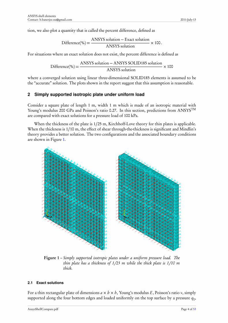
When the thickness of the plate is 1/25 m, Kirchhoff-Love theory for thin plates is applicable.When the thickness is 1/10 m, the effect of shear through-the-thickness is significant and Mindlin’stheory provides a better solution. The two configurations and the associated boundary conditionsare shown in Figure 1.
Figure 1 – Simply supported isotropic plates under a uniform pressure load. Thethin plate has a thickness of 1/25 m while the thick plate is 1/10 mthick.
2.1 Exact solutions
For a thin rectangular plate of dimensions a× b × h, Young’s modulus E , Poisson’s ratio ν, simplysupported along the four bottom edges and loaded uniformly on the top surface by a pressure q0,
AnsysShellCompare.pdf Page 4 of 53
ANSYS shell elementsContact: [email protected] 2011-July-13
the exact solution for the displacement, w(x, y), of the mid-surface is [1]
w(x, y) =∞∑
m=1
∞∑
n=1
16q0
(2m− 1)(2n− 1)π6D×
(2m− 1)2
a2+(2n− 1)2
b 2
−2
× sin(2m− 1)πx
asin(2n− 1)πy
b
(1)
where D = h3E/(12(1− ν2)). The resultant moment in the x-direction is
Mx x (x, y) =−D
∂ 2w
∂ x2+ ν
∂ 2w
∂ y2
!
.
Plugging in the expression for w(x, y), we get
Mx x (x, y) =∞∑
m=1
∞∑
n=1
16q0
(2m− 1)(2n− 1)π4
(2m− 1)2
a2+ ν(2n− 1)2
b 2
×
(2m− 1)2
a2+(2n− 1)2
b 2
−2
× sin(2m− 1)πx
asin(2n− 1)πy
b.
(2)
The bending stress in the plate is given by
σx x (x, y, z) =12z
h3Mx x (x, y) . (3)
For a thick plate subjected to the same boundary conditions, the exact solution for the mid-planedisplacement from Mindlin theory is [2, 3, 4]
w(x, y) =∞∑
m=1
∞∑
n=1
16q0
(2m− 1)(2n− 1)π6D×
(2m− 1)2
a2+(2n− 1)2
b 2
−2
× sin(2m− 1)πx
asin(2n− 1)πy
b×
(
1+π2h2
6κ(1− ν)
(2m− 1)2
a2+(2n− 1)2
b 2
)
(4)
The shear correction factor κ for a uniform cross-section is usually taken to be 5/6. We can find theresultant bending moment and shear force from the expression for w(x, y) for a simply supportedplate in a straightforward manner [4]. The expressions for these are
Mx x (x, y) =∞∑
m=1
∞∑
n=1
16q0
(2m− 1)(2n− 1)π4
(2m− 1)2
a2+ ν(2n− 1)2
b 2
×
(2m− 1)2
a2+(2n− 1)2
b 2
−2
× sin(2m− 1)πx
asin(2n− 1)πy
b,
(5)
AnsysShellCompare.pdf Page 5 of 53
ANSYS shell elementsContact: [email protected] 2011-July-13
and
Qz x (x, y) =∞∑
m=1
∞∑
n=1
16q0
(2n− 1)aπ3
(2m− 1)2
a2+(2n− 1)2
b 2
×
(2m− 1)2
a2+(2n− 1)2
b 2
−2
× cos(2m− 1)πx
asin(2n− 1)πy
b,
(6)
The bending and transverse shear stresses in the plate are given by
σx x (x, y, z) =12z
h3Mx x (x, y) and σz x (x, y, z) =
1
hκQz x (x, y)
1−4z2
h2
!
. (7)
2.2 The SHELL181 element
The SHELL181 element has 4 nodes with three translational and three rotational degrees of free-dom at each node and linear interpolation is used within the element. Several options are availablefor the element of which the number of integration points through the thickness (specified usingthe SECDATA command) and the in-plane integration algorithm (KEYOPT(3)={0,2}) are of inter-est for an isotropic plate. Other options, including the number of layers and anisotropic materialproperties will be discussed later in the report.
The displacement w at the bottom of the thin plate (along the line y = 0) and the stresses σx xat the top and bottom surfaces of the plate (at y = 0) are shown in Figure 2 (p. 8). These quantitiesare compared with the exact solution directly and also in terms of a percent difference defined as
Difference(%) =ANSYS solution−Exact solution
ANSYS solution× 100 .
The exact solution is shown by dashed lines. The solid lines are the simulated results. We canobserve the effect of mesh refinement on the displacement solution in parts a and b of the figure.A well-converged solution is obtained for n = 80, i.e., when there are 80 elements along an edge ofthe plate. The ANSYSTM result differs from the exact solution by 4%-6%. The stress solution isshown in parts c and d of the figure. The solution converges for n = 80 but there are large errors atthe edges of the plate where the ANSYSTM solution flattens out instead of reaching the zero stresscondition.
The effect of increasing the number of through-thickness integration points and of changing theKEYOPT value can be seen in parts e and f of the figure. These plots are for the n = 80 case. Theplots show that the effect of changing the number of integration points and the in-plane integrationalgorithm is negligible for a thin isotropic plate under uniform load.
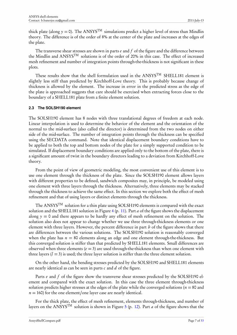
Figure 3 (p. 9) shows plots of the displacement (w), bending stress (σx x ), and transverse shearstress (σz x ) for the thicker plate. Differences between ANSYSTM results and exact (Mindlin) solu-tions are also shown in the Figure. Parts a and b of the figure show the effect of mesh refinement(n) and the number of through-thickness integration points (i ) on the displacement solution. TheKirchhoff-Love (K) solution is stiffer than the Mindlin (M) solution. However, the ANSYSTM so-lution shows a displacement that is approximately 10% greater than the exact solution, suggestingthat a higher-order plate theory is probably more appropriate for a plate thickness of h = a/10.Increasing the number of integration points and mesh refinement does not appear to affect thesolution significantly.
Parts c and d of the plot show the bending stresses along the top and bottom surfaces of the
AnsysShellCompare.pdf Page 6 of 53
ANSYS shell elementsContact: [email protected] 2011-July-13
thick plate (along y = 0). The ANSYSTM simulations predict a higher level of stress than Mindlintheory. The difference is of the order of 8% at the center of the plate and increases at the edges ofthe plate.
The transverse shear stresses are shown in parts e and f of the figure and the difference betweenthe Mindlin and ANSYSTM solutions is of the order of 20% in this case. The effect of increasedmesh refinement and number of integration points through-the-thickness is not significant in theseplots.
These results show that the shell formulation used in the ANSYSTM SHELL181 element isslightly less stiff than predicted by Kirchhoff-Love theory. This is probably because change ofthickness is allowed by the element. The increase in error in the predicted stress as the edge ofthe plate is approached suggests that care should be exercised when extracting forces close to theboundary of a SHELL181 plate from a finite element solution.
2.3 The SOLSH190 element
The SOLSH190 element has 8 nodes with three translational degrees of freedom at each node.Linear interpolation is used to determine the behavior of the element and the orientation of thenormal to the mid-surface (also called the director) is determined from the two nodes on eitherside of the mid-surface. The number of integration points through the thickness can be specifiedusing the SECDATA command. Note that identical displacement boundary conditions have tobe applied to both the top and bottom nodes of the plate for a simply supported condition to besimulated. If displacement boundary conditions are applied only to the bottom of the plate, there isa significant amount of twist in the boundary directors leading to a deviation from Kirchhoff-Lovetheory.
From the point of view of geometric modeling, the most convenient use of this element is touse one element through the thickness of the plate. Since the SOLSH190 element allows layerswith different properties to be defined, sandwich composites may, in principle, be modeled usingone element with three layers through the thickness. Alternatively, three elements may be stackedthrough the thickness to achieve the same effect. In this section we explore both the effect of meshrefinement and that of using layers or distinct elements through the thickness.
The ANSYSTM solution for a thin plate using SOLSH190 elements is compared with the exactsolution and the SHELL181 solution in Figure 4 (p. 11). Part a of the figure shows the displacementalong y = 0 and there appears to be hardly any effect of mesh refinement on the solution. Thesolution also does not appear to change whether we use three through-thickness elements or oneelement with three layers. However, the percent difference in part b of the figure shows that thereare differences between the various solutions. The SOLSH190 solution is reasonably convergedwhen the plate has n = 80 elements along an edge and one element through-the-thickness. Butthis converged solution is stiffer than that predicted by SHELL181 elements. Small differences areobserved when three elements (e = 3) are used through-the-thickness than when one element withthree layers (l = 3) is used; the three layer solution is stiffer than the three element solution.
On the other hand, the bending stresses predicted by the SOLSH190 and SHELL181 elementsare nearly identical as can be seen in parts c and d of the figure.
Parts e and f of the figure show the transverse shear stresses predicted by the SOLSH190 el-ement and compared with the exact solution. In this case the three element through-thicknesssolution predicts higher stresses at the edges of the plate while the converged solutions (n = 80 andn = 160) for the one element/one layer case are nearly identical.
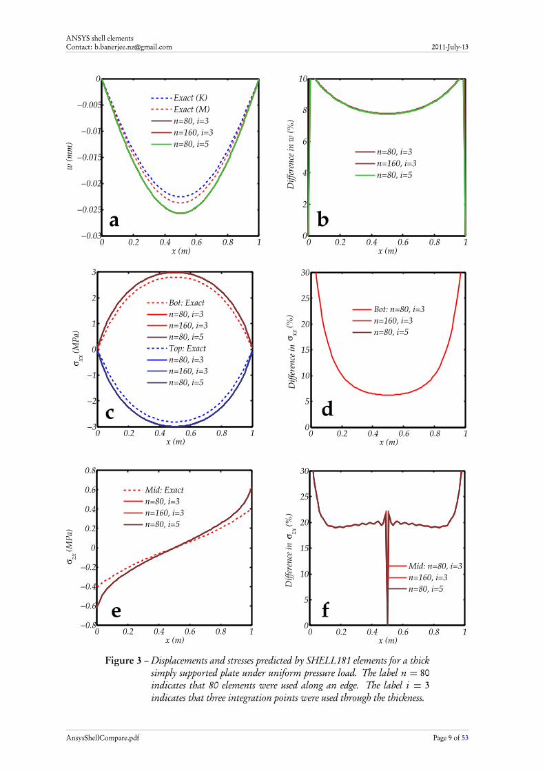
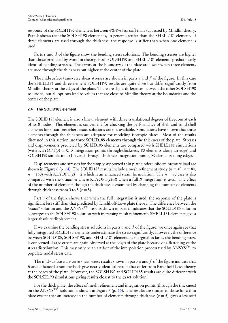
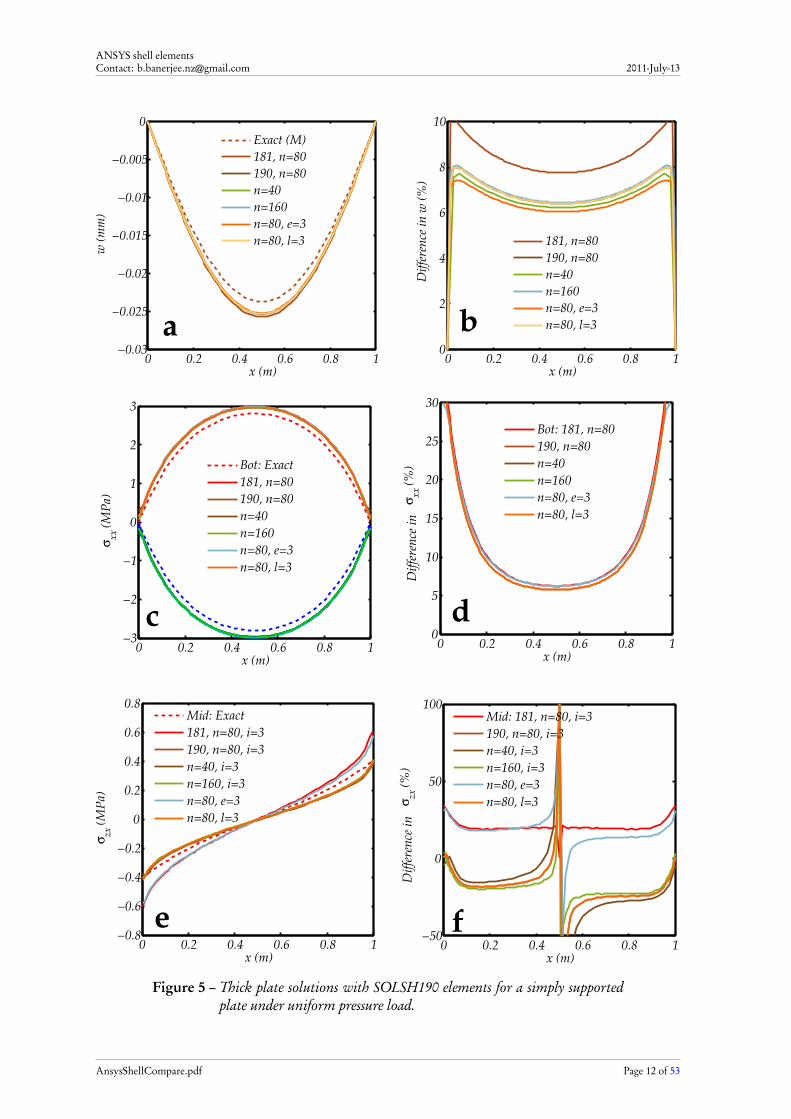
For the thick plate, the effect of mesh refinement, elements through-thickness, and number oflayers on the ANSYSTM solution is shown in Figure 5 (p. 12). Part a of the figure shows that the
AnsysShellCompare.pdf Page 7 of 53

ANSYS shell elementsContact: [email protected] 2011-July-13
0 0.2 0.4 0.6 0.8 1−0.4
−0.3
−0.2
−0.1
0
x (m)
w (
mm
)
Exact
n=40
n=80
n=160
0 0.2 0.4 0.6 0.8 1−20
−10
0
10
20
x (m)
σ
xx (
MP
a)
Bot: Exact
n=40
n=80
n=160
Top: Exact
n=40
n=80
n=160
0 0.2 0.4 0.6 0.8 10
2
4
6
8
10
x (m)
Dif
fere
nce
in
w (
%)
n=40
n=80
n=160
0 0.2 0.4 0.6 0.8 10
5
10
15
20
25
30
x (m)
Dif
fere
nce
in
σ
xx (
%) Bot: n=40
n=80
n=160
Top: n=40
n=80
n=160
ba
c d
0 0.2 0.4 0.6 0.8 10
2
4
6
8
10
x (m)
Dif
fere
nce
in
w (
%)
Keyopt(3)=0, Int. Pts.=3
Keyopt(3)=2, Int. Pts.=3
Keyopt(3)=0, Int. Pts.=5
0 0.2 0.4 0.6 0.8 10
5
10
15
20
25
30
x (m)
Dif
fere
nce
in
σxx
(%
)
Keyopt(3)=0, Int. Pts.=3
Keyopt(3)=2, Int. Pts.=3
Keyopt(3)=0, Int. Pts.=5
e f
Figure 2 – Effect of mesh refinement, KEYOPT values, and number of through-thickness integration points on solutions using SHELL181 elements fora thin simply supported plate under uniform pressure load.
AnsysShellCompare.pdf Page 8 of 53
ANSYS shell elementsContact: [email protected] 2011-July-13
0 0.2 0.4 0.6 0.8 1−0.03
−0.025
−0.02
−0.015
−0.01
−0.005
0
x (m)
w (
mm
)
Exact (K)
Exact (M)
n=80, i=3
n=160, i=3
n=80, i=5
0 0.2 0.4 0.6 0.8 10
2
4
6
8
10
x (m)
Dif
fere
nce
in
w (
%)
n=80, i=3
n=160, i=3
n=80, i=5
a b
0 0.2 0.4 0.6 0.8 1−3
−2
−1
0
1
2
3
x (m)
σxx
(M
Pa)
Bot: Exact
n=80, i=3
n=160, i=3
n=80, i=5
Top: Exact
n=80, i=3
n=160, i=3
n=80, i=5
0 0.2 0.4 0.6 0.8 1−0.8
−0.6
−0.4
−0.2
0
0.2
0.4
0.6
0.8
x (m)
σzx
(M
Pa)
Mid: Exact
n=80, i=3
n=160, i=3
n=80, i=5
0 0.2 0.4 0.6 0.8 10
5
10
15
20
25
30
x (m)
Dif
fere
nce
in
σxx
(%
)
Bot: n=80, i=3
n=160, i=3
n=80, i=5
0 0.2 0.4 0.6 0.8 10
5
10
15
20
25
30
x (m)
Dif
fere
nce
in
σzx
(%
)
Mid: n=80, i=3
n=160, i=3
n=80, i=5
c d
e f
Figure 3 – Displacements and stresses predicted by SHELL181 elements for a thicksimply supported plate under uniform pressure load. The label n = 80indicates that 80 elements were used along an edge. The label i = 3indicates that three integration points were used through the thickness.
AnsysShellCompare.pdf Page 9 of 53
ANSYS shell elementsContact: [email protected] 2011-July-13
response of the SOLSH190 element is between 6%-8% less stiff than suggested by Mindlin theory.Part b shows that the SOLSH190 element is, in general, stiffer than the SHELL181 element. Ifthree elements are used through the thickness, the response is stiffer than when one element isused.
Parts c and d of the figure show the bending stress solutions. The bending stresses are higherthan those predicted by Mindlin theory. Both SOLSH190 and SHELL181 elements predict nearlyidentical bending stresses. The errors at the boundary of the plate are lower when three elementsare used through the thickness but higher at the center of the plate.
The mid-surface transverse shear stresses are shown in parts e and f of the figure. In this casethe SHELL181 and three-element SOLSH190 results are quite close but differ significantly fromMindlin theory at the edges of the plate. There are slight differences between the other SOLSH190solutions, but all options lead to values that are close to Mindlin theory at the boundaries and thecenter of the plate.
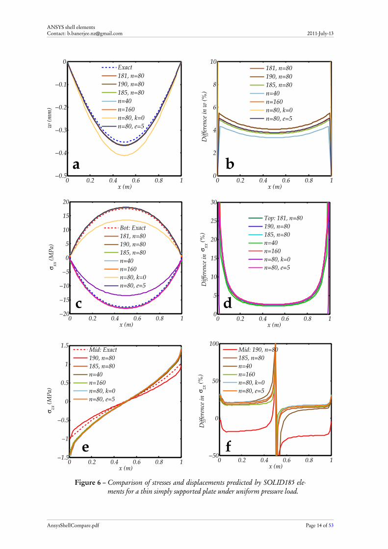
2.4 The SOLID185 element
The SOLID185 element is also a linear element with three translational degrees of freedom at eachof its 8 nodes. This element is convenient for checking the performance of shell and solid shellelements for situations where exact solutions are not available. Simulations have shown that threeelements through the thickness are adequate for modeling isotropic plates. Most of the resultsdiscussed in this section use three SOLID185 elements through the thickness of the plate. Stressesand displacements predicted by SOLID185 elements are compared with SHELL181 simulations(with KEYOPT(3) = 0, 3 integration points through-thickness, 80 elements along an edge) andSOLSH190 simulations (1 layer, 3 through-thickness integration points, 80 elements along edge).
Displacements and stresses for the simply supported thin plate under uniform pressure load areshown in Figure 6 (p. 14). The SOLID185 results include a mesh refinement study (n = 40, n = 80,n = 160) with KEYOPT(2) = 2 which is an enhanced strain formulation. The n = 80 case is alsocompared with the situation where KEYOPT(2)=0 when a full B̄ integration is used. The effectof the number of elements though the thickness is examined by changing the number of elementsthrough-thickness from 3 to 5 (e = 5).
Part a of the figure shows that when the full integration is used, the response of the plate issignificant less stiff than that predicted by Kirchhoff-Love plate theory. The difference between the“exact” solution and the ANSYSTM results shown in part b indicates that the SOLID185 solutionconverges to the SOLSH190 solution with increasing mesh refinement. SHELL181 elements give alarger absolute displacement.
If we examine the bending stress solutions in parts c and d of the figure, we once again see thatfully integrated SOLID185 elements underestimate the stress significantly. However, the differencebetween SOLID185, SOLSH190, and SHELL181 elements is marginal as far as the bending stressis concerned. Large errors are again observed at the edges of the plate because of a flattening of thestress distribution. This may only be an artifact of the interpolation process used by ANSYSTM topopulate nodal stress data.
The mid-surface transverse shear stress results shown in parts e and f of the figure indicate thatB̄ and enhanced strain methods give nearly identical results that differ from Kirchhoff-Love theoryat the edges of the plate. However, the SOLSH190 and SOLID185 results are quite different withthe SOLSH190 simulations giving results closest to the exact solution.
For the thick plate, the effect of mesh refinement and integration points (through the thickness)on the ANSYSTM solution is shown in Figure 7 (p. 15). The results are similar to those for a thinplate except that an increase in the number of elements through-thickness (e = 5) gives a less stiff
AnsysShellCompare.pdf Page 10 of 53

ANSYS shell elementsContact: [email protected] 2011-July-13
0 0.2 0.4 0.6 0.8 1−0.4
−0.35
−0.3
−0.25
−0.2
−0.15
−0.1
−0.05
0
x (m)
w (
mm
)
Exact
181, n=80
190, n=80
n=40
n=160
n=80, e=3
n=80, l=3
0 0.2 0.4 0.6 0.8 10
2
4
6
8
10
x (m)
Dif
fere
nce
in
w (
%)
181, n=80
190, n=80
n=40
n=160
n=80, e=3
n=80, l=3
a b
0 0.2 0.4 0.6 0.8 1−20
−15
−10
−5
0
5
10
15
20
x (m)
σxx
(M
Pa)
Bot: Exact
181, n=80
190, n=80
n=40
n=160
n=80, e=3
n=80, l=3
0 0.2 0.4 0.6 0.8 10
5
10
15
20
25
30
x (m)
Dif
fere
nce
in
σxx
(%
)Top: 181, n=80
190, n=80
n=40
n=160
n=80, e=3
n=80, l=3
0 0.2 0.4 0.6 0.8 1−1.5
−1
−0.5
0
0.5
1
1.5
x (m)
σzx
(M
Pa)
Mid: Exact
190, n=80, i=3
n=40, i=3
n=160, i=3
n=80, e=3
n=80, l=3
0 0.2 0.4 0.6 0.8 1−50
0
50
100
x (m)
Dif
fere
nce
in
σ
zx (
%)
Mid: 190, n=80, i=3
n=40, i=3
n=160, i=3
n=80, e=3
n=80, l=3
c d
e f
Figure 4 – Displacement and stresses in a thin plate modeled with SOLSH190 ele-ments under a uniform pressure load. The effect of mesh refinement, thenumber of elements through-thickness, and the number of layers in anelements can be observed from the plots.
AnsysShellCompare.pdf Page 11 of 53
ANSYS shell elementsContact: [email protected] 2011-July-13
0 0.2 0.4 0.6 0.8 1−0.03
−0.025
−0.02
−0.015
−0.01
−0.005
0
x (m)
w (
mm
)
Exact (M)
181, n=80
190, n=80
n=40
n=160
n=80, e=3
n=80, l=3
0 0.2 0.4 0.6 0.8 10
2
4
6
8
10
x (m)
Dif
fere
nce
in
w (
%)
181, n=80
190, n=80
n=40
n=160
n=80, e=3
n=80, l=3a b
0 0.2 0.4 0.6 0.8 1−3
−2
−1
0
1
2
3
x (m)
σxx
(M
Pa)
Bot: Exact
181, n=80
190, n=80
n=40
n=160
n=80, e=3
n=80, l=3
0 0.2 0.4 0.6 0.8 10
5
10
15
20
25
30
x (m)
Dif
fere
nce
in
σ
xx (
%)
Bot: 181, n=80
190, n=80
n=40
n=160
n=80, e=3
n=80, l=3
0 0.2 0.4 0.6 0.8 1−0.8
−0.6
−0.4
−0.2
0
0.2
0.4
0.6
0.8
x (m)
σzx
(M
Pa)
Mid: Exact
181, n=80, i=3
190, n=80, i=3
n=40, i=3
n=160, i=3
n=80, e=3
n=80, l=3
0 0.2 0.4 0.6 0.8 1−50
0
50
100
x (m)
Dif
fere
nce
in
σ
zx (
%)
Mid: 181, n=80, i=3
190, n=80, i=3
n=40, i=3
n=160, i=3
n=80, e=3
n=80, l=3
c d
e f
Figure 5 – Thick plate solutions with SOLSH190 elements for a simply supportedplate under uniform pressure load.
AnsysShellCompare.pdf Page 12 of 53

ANSYS shell elementsContact: [email protected] 2011-July-13
solution than SOLSH190 elements and three SOLID185 elements through the thickness.
AnsysShellCompare.pdf Page 13 of 53
ANSYS shell elementsContact: [email protected] 2011-July-13
0 0.2 0.4 0.6 0.8 1−0.5
−0.4
−0.3
−0.2
−0.1
0
x (m)
w (
mm
)
Exact
181, n=80
190, n=80
185, n=80
n=40
n=160
n=80, k=0
n=80, e=5
0 0.2 0.4 0.6 0.8 10
2
4
6
8
10
x (m)
Dif
fere
nce
in
w (
%)
181, n=80
190, n=80
185, n=80
n=40
n=160
n=80, k=0
n=80, e=5
a b
0 0.2 0.4 0.6 0.8 1−20
−15
−10
−5
0
5
10
15
20
x (m)
σxx
(M
Pa)
Bot: Exact
181, n=80
190, n=80
185, n=80
n=40
n=160
n=80, k=0
n=80, e=5
0 0.2 0.4 0.6 0.8 10
5
10
15
20
25
30
x (m)
Dif
fere
nce
in
σxx
(%
)
Top: 181, n=80
190, n=80
185, n=80
n=40
n=160
n=80, k=0
n=80, e=5
0 0.2 0.4 0.6 0.8 1−1.5
−1
−0.5
0
0.5
1
1.5
x (m)
σzx
(M
Pa)
Mid: Exact
190, n=80
185, n=80
n=40
n=160
n=80, k=0
n=80, e=5
0 0.2 0.4 0.6 0.8 1−50
0
50
100
x (m)
Dif
fere
nce
in
σzx
(%
)
Mid: 190, n=80
185, n=80
n=40
n=160
n=80, k=0
n=80, e=5
c d
e f
Figure 6 – Comparison of stresses and displacements predicted by SOLID185 ele-ments for a thin simply supported plate under uniform pressure load.
AnsysShellCompare.pdf Page 14 of 53

ANSYS shell elementsContact: [email protected] 2011-July-13
0 0.2 0.4 0.6 0.8 1−0.03
−0.025
−0.02
−0.015
−0.01
−0.005
0
x (m)
w (
mm
)
Exact (M)
181, n=80
190, n=80
185, n=80
n=40
n=160
n=80, k=0
n=80, e=5
0 0.2 0.4 0.6 0.8 10
2
4
6
8
10
x (m)
Dif
fere
nce
in
w (
%)
a b
0 0.2 0.4 0.6 0.8 1−4
−3
−2
−1
0
1
2
3
4
x (m)
σxx
(M
Pa)
Bot: Exact
181, n=80
190, n=80
185, n=80
n=40
n=160
n=80, k=0
n=80, e=5
0 0.2 0.4 0.6 0.8 10
5
10
15
20
25
30
x (m)
Dif
fere
nce
in
σxx
(%
)
0 0.2 0.4 0.6 0.8 1−0.8
−0.6
−0.4
−0.2
0
0.2
0.4
0.6
0.8
x (m)
σzx
(M
Pa)
Mid: Exact
181, n=80
190, n=80
185, n=80
n=40
n=160
n=80, k=0
n=80, e=5
0 0.2 0.4 0.6 0.8 1−50
0
50
100
x (m)
Dif
fere
nce
in
σzx
(%
)
c d
e f
Figure 7 – Solutions for a thick simply supported plate under uniform pressure loadusing SOLID185 elements.
AnsysShellCompare.pdf Page 15 of 53

ANSYS shell elementsContact: [email protected] 2011-July-13
3 Isotropic plate loaded by boundary moments
Another problem for which analytical solutions are readily available is the situation where anisotropic plate is loaded by boundary moments. In this section we compare the analytical solu-tion from Kirchhoff-Love theory with ANSYSTM solutions using SHELL181, SOLSH190, andSOLID185 elements. The plate is square (1 m long) and made of an isotropic material with Young’smodulus 200 GPa and Poisson’s ratio 0.27. The thickness of the plate is 1/25 m. The four edges ofthe plate are simply supported. The edges at y = −b/2 and y = b/2 are loaded with a boundarymoment of 10 kN-m as shown in Figure 8.
Figure 8 – Simply supported isotropic plate under uniform moment loads alongtwo opposite edges.
3.1 Exact solutions
For a thin rectangular plate loaded by a uniform edge moment M0, the exact solution for the trans-verse displacement is [1]
w(x, y) =2M0a2
π3D
∞∑
m=1
1
(2m− 1)3 coshαm
sin(2m− 1)πx
a×
�
αm tanhαm cosh(2m− 1)πy
a−(2m− 1)πy
asinh
(2m− 1)πy
a
�
where
αm =π(2m− 1)b
2a.
AnsysShellCompare.pdf Page 16 of 53
ANSYS shell elementsContact: [email protected] 2011-July-13
The bending moment resultants are
Mx x (x, y) =2M0(1− ν)
π
∞∑
m=1
1
(2m− 1)coshαmsin(2m− 1)πx
a
�
−(2m− 1)πy
asinh
(2m− 1)πy
a+
� 2ν
1− ν+αm tanhαm
�
cosh(2m− 1)πy
a
�
Myy (x, y) =2M0(1− ν)
π
∞∑
m=1
1
(2m− 1)coshαmsin(2m− 1)πx
a
�
(2m− 1)πy
asinh
(2m− 1)πy
a+
� 2
1− ν−αm tanhαm
�
cosh(2m− 1)πy
a
�
and the shear force resultants are
Qz x (x, y) =4M0
a
∞∑
m=1
1
coshαmcos(2m− 1)πx
acosh
(2m− 1)πy
a
Qy z (x, y) =4M0
a
∞∑
m=1
1
coshαmsin(2m− 1)πx
asinh
(2m− 1)πy
a.
The stresses are
σx x =12z
h3Mx x , σyy =
12z
h3Myy , σz x =
1
κhQz x
1−4z2
h2
!
and σy z =1
κhQy z
1−4z2
h2
!
.
3.2 SHELL181 element
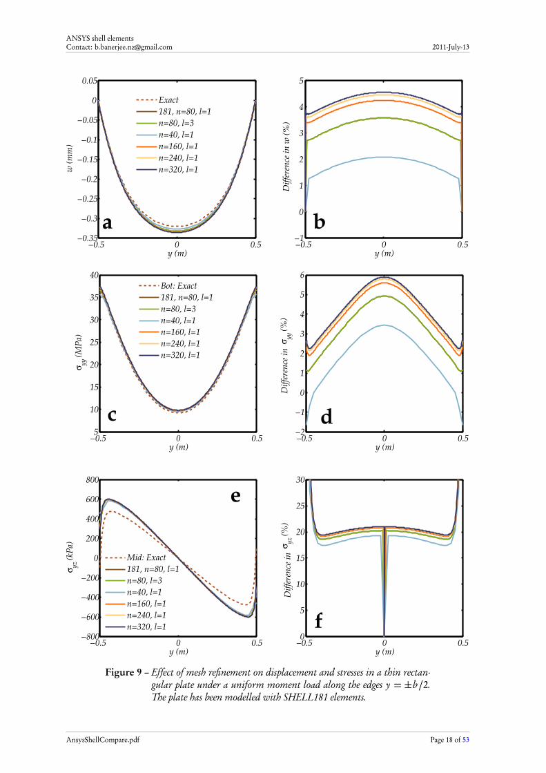
Figure 9 (p. 18) shows plots of the transverse displacement, the bottom-surface bending stress, andthe mid-surface transverse shear stress in the plate along the line x = a/2. The results show that thesolution converges with mesh refinement. However, convergence is slower than for the situationwhere a uniform pressure is applied to the plate. The error at the edge of the plate appears toincrease with increased refinement. Most of the results are for the case where a single layer (l = 1)is used through the plate thickness. Results are identical when three layers (l = 3) of identicalthickness are used instead.
The difference between the ANSYSTM solution and the exact results are less than 6% for thedisplacement (w) and the bending stress (σyy ). However, as can be seen in parts e and f of thefigure, there is a large difference between the ANSYSTM solution for the transverse shear stress(σy z ) and that predicted by Kirchhoff-Love theory, even though the trend is similar.
3.3 SOLSH190 element
When SOLSH190 elements are used to model the plate, moments cannot be applied directly tothe edges of the plate. Instead, forces of equal magnitude but opposite sign can be applied to thetop and bottom edges of the plate when one element is used to model the thickness of the plate.Alternatively, a gradient surface force distribution of peak magnitude 6M0/h2 and slope 12M0/h3
can be applied to the edge areas (identified as b c = 2 in the plots).
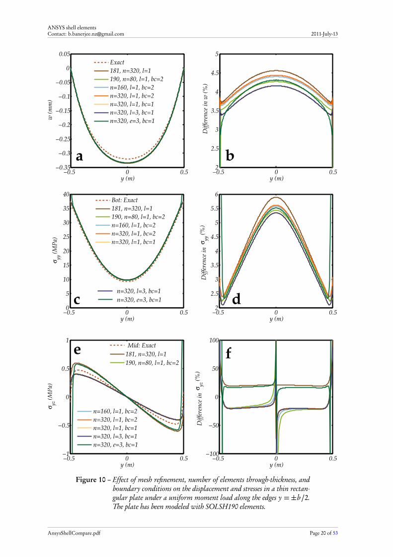
Figure 10 (p. 20) shows plots of the transverse displacements, bending stresses, and transverseshear stresses for a plate modeled with SOLSH190 elements. In general, as shown in part a of the fig-ure, the ANSYSTM displacements are larger than the predicted values from Kirchhoff-Love theory.From part b of the figure we can see that the displacements obtained using SOLSH190 elements
AnsysShellCompare.pdf Page 17 of 53
ANSYS shell elementsContact: [email protected] 2011-July-13
−0.5 0 0.5−0.35
−0.3
−0.25
−0.2
−0.15
−0.1
−0.05
0
0.05
y (m)
w (
mm
)
Exact
181, n=80, l=1
n=80, l=3
n=40, l=1
n=160, l=1
n=240, l=1
n=320, l=1
−0.5 0 0.5−1
0
1
2
3
4
5
y (m)
Dif
fere
nce
in
w (
%)
a b
−0.5 0 0.55
10
15
20
25
30
35
40
y (m)
σyy
(M
Pa)
Bot: Exact
181, n=80, l=1
n=80, l=3
n=40, l=1
n=160, l=1
n=240, l=1
n=320, l=1
−0.5 0 0.5−2
−1
0
1
2
3
4
5
6
y (m)
Dif
fere
nce
in
σyy
(%
)
−0.5 0 0.5−800
−600
−400
−200
0
200
400
600
800
y (m)
σyz
(kP
a)
Mid: Exact
181, n=80, l=1
n=80, l=3
n=40, l=1
n=160, l=1
n=240, l=1
n=320, l=1
−0.5 0 0.50
5
10
15
20
25
30
y (m)
Dif
fere
nce
in
σyz
(%
)
c d
e
f
Figure 9 – Effect of mesh refinement on displacement and stresses in a thin rectan-gular plate under a uniform moment load along the edges y = ±b/2.The plate has been modelled with SHELL181 elements.
AnsysShellCompare.pdf Page 18 of 53
ANSYS shell elementsContact: [email protected] 2011-July-13
are smaller than those predicted by SHELL181 elements (the difference is largest for SHELL181elements). The SOLSH190 results converge rapidly beyond a mesh refinement of 160 elements peredge (n = 160) if a gradient surface force is applied along the edges (b c = 2). Instead, if forces areapplied directly (b c = 1), the predicted displacements are significantly lower. The effect of the num-ber of layers (l = 1 or l = 3) is negligible, but three elements through-thickness (e = 3) leads to a lessstiff response and significant edge effects unless a gradient surface load is used to apply moments.
Part c of the figure indicates that the bending stresses predicted by ANSYSTM are lower thanthose given by Kirchhoff-Love theory. The smallest stresses are those using SHELL181 elementsand the largest are from SOLSH190 elements with nodal force boundary conditions. The differ-ences are largest at the center of the plate and smallest near the edges (see part d of the figure).
The transverse shear stresses (parts e and f of the figure) predicted by SHELL181 elements andSOLSH190 elements with three elements through-thickness are nearly identical and the percent dif-ference is greater than zero for both these cases. However, for the single and three-layer SOLSH190simulations, the shear stresses appear to be unaffected by the applied boundary conditions and theseare always lower than the exact solution (in absolute value).
AnsysShellCompare.pdf Page 19 of 53
ANSYS shell elementsContact: [email protected] 2011-July-13
−0.5 0 0.5−0.35
−0.3
−0.25
−0.2
−0.15
−0.1
−0.05
0
0.05
y (m)
w (
mm
)
Exact
181, n=320, l=1
190, n=80, l=1, bc=2
n=160, l=1, bc=2
n=320, l=1, bc=2
n=320, l=1, bc=1
n=320, l=3, bc=1
n=320, e=3, bc=1
−0.5 0 0.52
2.5
3
3.5
4
4.5
5
y (m)
Dif
fere
nce
in
w (
%)
a b
−0.5 0 0.50
5
10
15
20
25
30
35
40
y (m)
σyy
(M
Pa)
Bot: Exact
181, n=320, l=1
190, n=80, l=1, bc=2
n=160, l=1, bc=2
n=320, l=1, bc=2
n=320, l=1, bc=1
n=320, l=3, bc=1
n=320, e=3, bc=1
−0.5 0 0.52
2.5
3
3.5
4
4.5
5
5.5
6
y (m)
Dif
fere
nce
in
σyy
(%
)
−0.5 0 0.5−1
−0.5
0
0.5
1
y (m)
σyz
(M
Pa)
Mid: Exact
181, n=320, l=1
190, n=80, l=1, bc=2
n=160, l=1, bc=2
n=320, l=1, bc=2
n=320, l=1, bc=1
n=320, l=3, bc=1
n=320, e=3, bc=1
−0.5 0 0.5−100
−50
0
50
100
y (m)
Dif
fere
nce
in
σyz
(%
)
e f
c d
Figure 10 – Effect of mesh refinement, number of elements through-thickness, andboundary conditions on the displacement and stresses in a thin rectan-gular plate under a uniform moment load along the edges y = ±b/2.The plate has been modeled with SOLSH190 elements.
AnsysShellCompare.pdf Page 20 of 53
ANSYS shell elementsContact: [email protected] 2011-July-13
4 Isotropic cantilever plate with concentrated edge load
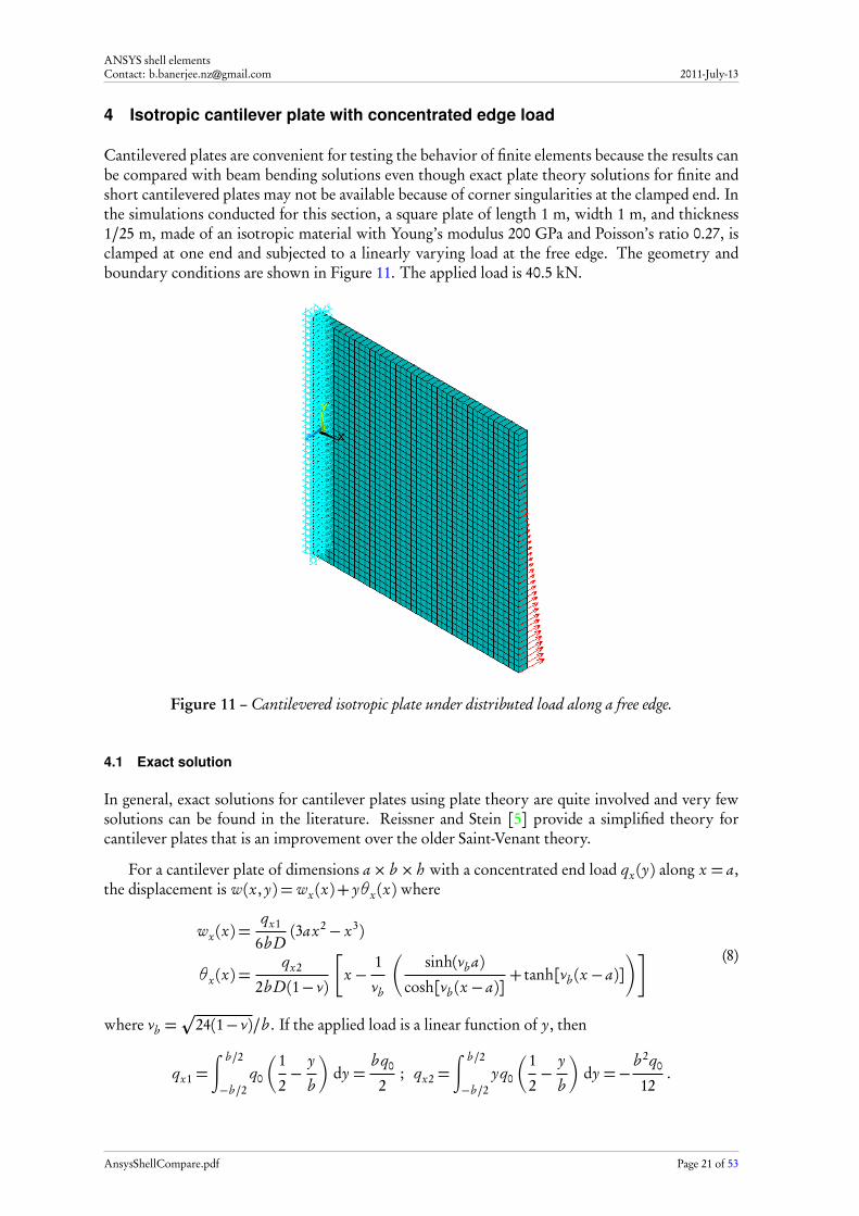
Cantilevered plates are convenient for testing the behavior of finite elements because the results canbe compared with beam bending solutions even though exact plate theory solutions for finite andshort cantilevered plates may not be available because of corner singularities at the clamped end. Inthe simulations conducted for this section, a square plate of length 1 m, width 1 m, and thickness1/25 m, made of an isotropic material with Young’s modulus 200 GPa and Poisson’s ratio 0.27, isclamped at one end and subjected to a linearly varying load at the free edge. The geometry andboundary conditions are shown in Figure 11. The applied load is 40.5 kN.
Figure 11 – Cantilevered isotropic plate under distributed load along a free edge.
4.1 Exact solution
In general, exact solutions for cantilever plates using plate theory are quite involved and very fewsolutions can be found in the literature. Reissner and Stein [5] provide a simplified theory forcantilever plates that is an improvement over the older Saint-Venant theory.
For a cantilever plate of dimensions a× b × h with a concentrated end load qx (y) along x = a,the displacement is w(x, y) = wx (x)+ yθx (x) where
wx (x) =qx1
6b D(3ax2− x3)
θx (x) =qx2
2b D(1− ν)
�
x −1
νb
�
sinh(νb a)
cosh[νb (x − a)]+ tanh[νb (x − a)]
�� (8)
where νb =p
24(1− ν)/b . If the applied load is a linear function of y, then
qx1 =∫ b/2
−b/2q0
�1
2−
y
b
�
dy =b q0
2; qx2 =
∫ b/2
−b/2yq0
�1
2−
y
b
�
dy =−b 2q0
12.
AnsysShellCompare.pdf Page 21 of 53
ANSYS shell elementsContact: [email protected] 2011-July-13
The resultant bending moments and shear forces are
Mx x =−D
∂ 2w
∂ x2+ ν
∂ 2w
∂ y2
!
= qx1
� x − a
b
�
−
3yqx2
b 3νb cosh3[νb (x − a)]
�
6sinh(νb a)− sinh[νb (2x − a)]+ sinh[νb (2x − 3a)]+ 8sinh[νb (x − a)]�
Mxy = (1− ν)D∂ 2w
∂ x∂ y
=qx2
2b
1−2+ cosh[νb (x − 2a)]− cosh[νb x]
2cosh2[νb (x − a)]
Qz x =∂ Mx x
∂ x−∂ Mxy
∂ y
=qx1
b−
3yqx2
2b 3 cosh4[νb (x − a)]
!
�
32+ cosh[νb (3x − 2a)]− cosh[νb (3x − 4a)]
−16cosh[2νb (x − a)]+ 23cosh[νb (x − 2a)]− 23cosh(νb x)�
.
(9)
The stresses are
σx x =12z
h3Mx x and σz x =
1
κhQz x
1−4z2
h2
!
.
If the applied load at the edge is constant, we recover the solutions for a beam under a concentratedend load.
4.2 SHELL181 element
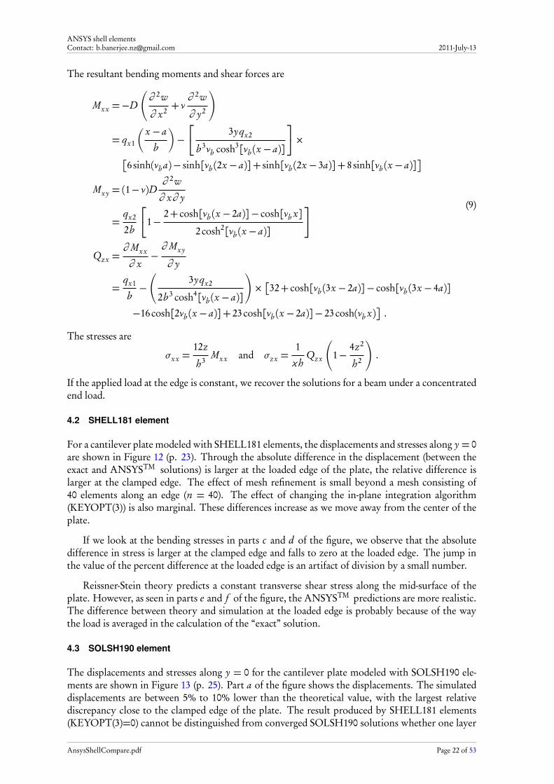
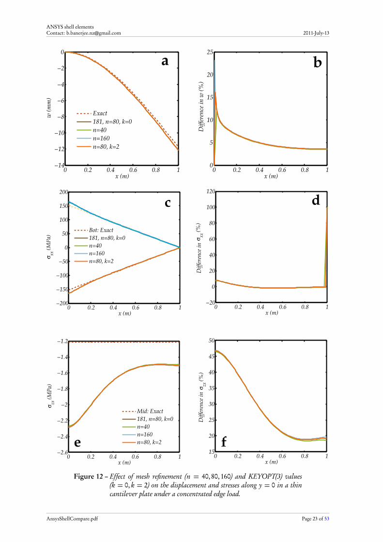
For a cantilever plate modeled with SHELL181 elements, the displacements and stresses along y = 0are shown in Figure 12 (p. 23). Through the absolute difference in the displacement (between theexact and ANSYSTM solutions) is larger at the loaded edge of the plate, the relative difference islarger at the clamped edge. The effect of mesh refinement is small beyond a mesh consisting of40 elements along an edge (n = 40). The effect of changing the in-plane integration algorithm(KEYOPT(3)) is also marginal. These differences increase as we move away from the center of theplate.
If we look at the bending stresses in parts c and d of the figure, we observe that the absolutedifference in stress is larger at the clamped edge and falls to zero at the loaded edge. The jump inthe value of the percent difference at the loaded edge is an artifact of division by a small number.
Reissner-Stein theory predicts a constant transverse shear stress along the mid-surface of theplate. However, as seen in parts e and f of the figure, the ANSYSTM predictions are more realistic.The difference between theory and simulation at the loaded edge is probably because of the waythe load is averaged in the calculation of the “exact” solution.
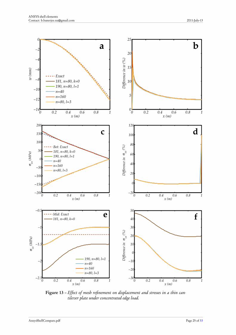
4.3 SOLSH190 element
The displacements and stresses along y = 0 for the cantilever plate modeled with SOLSH190 ele-ments are shown in Figure 13 (p. 25). Part a of the figure shows the displacements. The simulateddisplacements are between 5% to 10% lower than the theoretical value, with the largest relativediscrepancy close to the clamped edge of the plate. The result produced by SHELL181 elements(KEYOPT(3)=0) cannot be distinguished from converged SOLSH190 solutions whether one layer
AnsysShellCompare.pdf Page 22 of 53
ANSYS shell elementsContact: [email protected] 2011-July-13
0 0.2 0.4 0.6 0.8 1−14
−12
−10
−8
−6
−4
−2
0
x (m)
w (
mm
)
Exact
181, n=80, k=0
n=40
n=160
n=80, k=2
0 0.2 0.4 0.6 0.8 10
5
10
15
20
25
x (m)
Dif
fere
nce
in
w (
%)
ba
0 0.2 0.4 0.6 0.8 1−200
−150
−100
−50
0
50
100
150
200
x (m)
σxx
(M
Pa)
Bot: Exact
181, n=80, k=0
n=40
n=160
n=80, k=2
0 0.2 0.4 0.6 0.8 1−20
0
20
40
60
80
100
120
x (m)
Dif
fere
nce
in
σxx
(%
)
0 0.2 0.4 0.6 0.8 1−2.6
−2.4
−2.2
−2
−1.8
−1.6
−1.4
−1.2
x (m)
σzx
(M
Pa)
Mid: Exact
181, n=80, k=0
n=40
n=160
n=80, k=2
0 0.2 0.4 0.6 0.8 115
20
25
30
35
40
45
50
x (m)
Dif
fere
nce
in
σzx
(%
)c d
e f
Figure 12 – Effect of mesh refinement (n = 40,80,160) and KEYOPT(3) values(k = 0, k = 2) on the displacement and stresses along y = 0 in a thincantilever plate under a concentrated edge load.
AnsysShellCompare.pdf Page 23 of 53
ANSYS shell elementsContact: [email protected] 2011-July-13
(l = 1) or three layers (l = 3) are used. Convergence occurs rapidly and a mesh with 40 elementsto an edge (n = 40) gives results that are close to those for a mesh with 160 elements to an edge(n = 160).
Bending stresses predicted by ANSYSTM simulations are also nearly identical to the Reissner-Stein solution expect at the clamped end where the simulated results appear to be more accurate.The stresses along the bottom and top of the plate and the relative difference between ANSYSTM
and theoretical results are shown in parts c and d of the figure, respectively. The difference isobserved to be close to zero for all the cases explored.
However, as can be seen in parts e and f of the figure, the transverse shear stresses predicted bySHELL181 elements have significantly larger magnitudes (in absolute terms) than those predictedby SOLSH190 elements. The average shear stress along a cross-section (y = 0 in this case) fromSOLSH190 elements is close to the value predicted by Reissner-Stein theory and appears to bemore accurate.
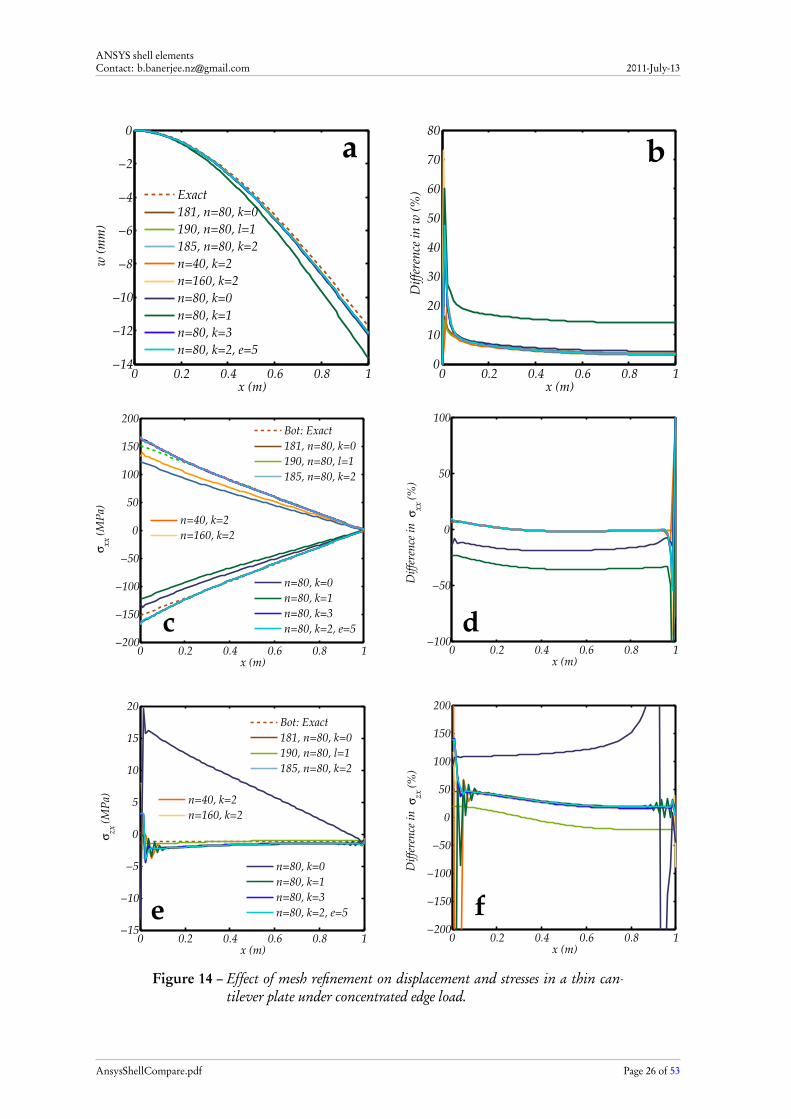
4.4 SOLID185 element
Given that the Reissner-Stein theory does not appear to be very accurate, it is critical that the resultsfrom SHELL181 and SOLSH190 simulations be checked with full three-dimensional simulationswith SOLID185 elements. There are several integration and element formulation options availablefor SOLID185 elements that can be accessed using KEYOPT(2). When this option is set to 0 (k = 0),the element is fully integrated and has the tendency to lock when used to model thin structures.The option 1 (k = 1) selects uniform reduced integration with hourglass control. Option 2 (k =2) activates an enhanced strain formulation and option 3 (k = 3) is a simplified enhanced strainformulation. All these options have been explored and the results are shown in Figure 14 (p. 26).We have also explored the effect of mesh refinement in the plane of the plate (n = 40,80,160)and through the thickness (e = 3,5, indicating the number of through-thickness elements). TheSOLID185 results are compared with the Reissner-Stein solution and results using SHELL181 andSOLSH190 elements.
The outlier curve in part a of the figure corresponds to the case (n = 80, k = 1) where uniformreduced integration has been used. The response of the plate is excessively compliant when thisoption is used. All the other curves in the plot are nearly identical but lower than the Reissner-Stein solution as can be seen in part b of the figure. These results indicate that the three elementtypes give us nearly identical values for the displacement.
Differences between various options become more obvious when we look at the bending stresscurves in parts c and d of the figure. In this case we have two clear outliers, the cases n = 80, k = 0and n = 80, k = 1. We have already discussed the k = 1 case which involves reduced integration.The k = 0 case involves full integration and predicted stresses that are lower than the Reissner-Stein estimate. All the other simulations give nearly identical results which are higher than thosepredicted by Reissner-Stein theory at the clamped edge. This indicates that the theoretical resultsare an underestimate of the actual stresses close to the clamped edge.
The error in the stresses predicted by fully integrated elements becomes clearer when we exam-ine the transverse shear stresses in parts e and f of the figure. The difference between the SOLID185prediction and the Reissner-Stein solution is of the order of 100% of the predicted value. Anothernew outlier appears in the results, shown by the light green line in part f . This case correspondsto the SOLSH190 calculation which is the closest to the theoretical value. However, all the otherSOLID185 simulations indicate that the shear stress should be close to the value predicted by theSHELL181 elements. This suggests that the SOLSH190 elements is less accurate than SHELL181elements when 1 layer/1 element is used through the thickness. Increasing the number of elementsthrough the thickness (e = 5) tends to smooth out fluctuations at the boundaries.
AnsysShellCompare.pdf Page 24 of 53
ANSYS shell elementsContact: [email protected] 2011-July-13
0 0.2 0.4 0.6 0.8 1−14
−12
−10
−8
−6
−4
−2
0
x (m)
w (
mm
)
Exact
181, n=80, k=0
190, n=80, l=1
n=40
n=160
n=80, l=3
0 0.2 0.4 0.6 0.8 10
5
10
15
20
25
x (m)
Dif
fere
nce
in
w (
%)
a b
0 0.2 0.4 0.6 0.8 1−200
−150
−100
−50
0
50
100
150
200
x (m)
σxx
(M
Pa)
Bot: Exact
181, n=80, k=0
190, n=80, l=1
n=40
n=160
n=80, l=3
0 0.2 0.4 0.6 0.8 1−20
0
20
40
60
80
100
120
x (m)
Dif
fere
nce
in
σ
xx (
%)
0 0.2 0.4 0.6 0.8 1−2.5
−2
−1.5
−1
−0.5
x (m)
σzx
(M
Pa)
Mid: Exact
181, n=80, k=0
190, n=80, l=1
n=40
n=160
n=80, l=3
0 0.2 0.4 0.6 0.8 1−30
−20
−10
0
10
20
30
40
50
x (m)
Dif
fere
nce
in
σ
zx (
%)
c
e f
d
Figure 13 – Effect of mesh refinement on displacement and stresses in a thin can-tilever plate under concentrated edge load.
AnsysShellCompare.pdf Page 25 of 53
ANSYS shell elementsContact: [email protected] 2011-July-13
0 0.2 0.4 0.6 0.8 1−14
−12
−10
−8
−6
−4
−2
0
x (m)
w (
mm
)
Exact
181, n=80, k=0
190, n=80, l=1
185, n=80, k=2
n=40, k=2
n=160, k=2
n=80, k=0
n=80, k=1
n=80, k=3
n=80, k=2, e=5
0 0.2 0.4 0.6 0.8 10
10
20
30
40
50
60
70
80
x (m)
Dif
fere
nce
in
w (
%)
a b
0 0.2 0.4 0.6 0.8 1−200
−150
−100
−50
0
50
100
150
200
x (m)
σxx
(M
Pa)
Bot: Exact
Bot: Exact
181, n=80, k=0
181, n=80, k=0
190, n=80, l=1
190, n=80, l=1
185, n=80, k=2
185, n=80, k=2
n=40, k=2
n=40, k=2
n=160, k=2
n=160, k=2
n=80, k=0
n=80, k=0
n=80, k=1
n=80, k=1
n=80, k=3
n=80, k=3
n=80, k=2, e=5
n=80, k=2, e=5
0 0.2 0.4 0.6 0.8 1−100
−50
0
50
100
x (m)
Dif
fere
nce
in
σxx
(%
)
0 0.2 0.4 0.6 0.8 1−15
−10
−5
0
5
10
15
20
x (m)
σzx
(M
Pa)
0 0.2 0.4 0.6 0.8 1−200
−150
−100
−50
0
50
100
150
200
x (m)
Dif
fere
nce
in
σ
zx (
%)
c d
e f
Figure 14 – Effect of mesh refinement on displacement and stresses in a thin can-tilever plate under concentrated edge load.
AnsysShellCompare.pdf Page 26 of 53

ANSYS shell elementsContact: [email protected] 2011-July-13
5 Cantilever orthotropic plate with concentrated edge load
The simulations in the previous section showed that SHELL181 and SOLSH190 elements predictedslightly different stresses. In this section we examine whether these differences are magnified whenthe plate is thicker and made of an orthotropic material. The plate thickness is 1/10 m and thematerial properties are Ex x = Eyy = 17.3 GPa, Ez z = 3.24 GPa, Gxy = 6.7 GPa, Gy z = Gz x = 1.2GPa, νx z = νy z = 0.32. The applied load is the same as in the previous section. A plot of thegeometry and boundary conditions is shown in Figure 15. Since exact solutions for an orthotropiccantilevered plate are not available, comparisons have been made with the Reissner-Stein solutionsfor an isotropic plate with E = 17.3 GPa and G = 6.7 GPa. These solutions for an isotropic platehave been labelled “exact” in the plots that follow.
Figure 15 – Cantilevered orthotropic plate under distributed load along a free edge.
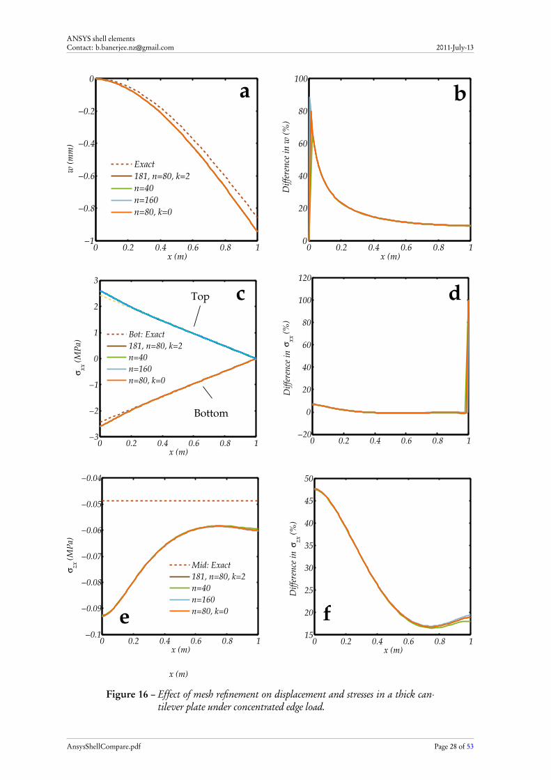
5.1 SHELL181 element
The displacements and stresses along y = 0 for the cantilever plate modeled with SHELL181 ele-ments are shown in Figure 16 (p. 28). Convergence of the displacement solution is rapid as seen inparts a and b of the figure. The predicted displacements are larger than those for an isotropic plate,partly because rotation of the mid-surface normals due to shear has not been considered in the ex-act solution. No differences are observed when the options KEYOPT(3)=0 and KEYOPT(3)=2are interchanged.
Interestingly, the bending stresses shown in parts c and d of the figure are remarkably close tothat for an isotropic plate. A small discrepancy, similar to that observed in the previous section,can be seen at the clamped edge. The shear stress along y = 0 at the mid-surface is shown in partse and f of the figure. Once again, there is a high shear stress at the clamped edge compared to theloaded edge. Also, convergence is slower close to the loaded edge compared to the clamped edge.
AnsysShellCompare.pdf Page 27 of 53
ANSYS shell elementsContact: [email protected] 2011-July-13
0 0.2 0.4 0.6 0.8 1−1
−0.8
−0.6
−0.4
−0.2
0
x (m)
w (
mm
)
Exact
181, n=80, k=2
n=40
n=160
n=80, k=0
0 0.2 0.4 0.6 0.8 10
20
40
60
80
100
x (m)
Dif
fere
nce
in
w (
%)
a b
0 0.2 0.4 0.6 0.8 1−3
−2
−1
0
1
2
3
x (m)
σxx
(M
Pa)
Bot: Exact
181, n=80, k=2
n=40
n=160
n=80, k=0
0 0.2 0.4 0.6 0.8 1−20
0
20
40
60
80
100
120
x (m)
Dif
fere
nce
in
σxx
(%
)
0 0.2 0.4 0.6 0.8 1−0.1
−0.09
−0.08
−0.07
−0.06
−0.05
−0.04
x (m)
σzx
(M
Pa)
Mid: Exact
181, n=80, k=2
n=40
n=160
n=80, k=0
0 0.2 0.4 0.6 0.8 115
20
25
30
35
40
45
50
x (m)
Dif
fere
nce
in
σzx
(%
)dc
e f
Bottom
Top
Figure 16 – Effect of mesh refinement on displacement and stresses in a thick can-tilever plate under concentrated edge load.
AnsysShellCompare.pdf Page 28 of 53
ANSYS shell elementsContact: [email protected] 2011-July-13
5.2 SOLSH190 element
Corresponding plots for simulations with SOLSH190 elements are shown in Figure 17 (p. 30). Thedisplacements along y = 0 converge rapidly, are similar to those predicted by SHELL181 elements,and are not affected significantly whether one layer (l = 1), three layers (l = 3), or three elementsare used (e = 3) through the thickness. The three-element solution is slightly more compliant thanthe one-element solution (with one or three layers).
Parts c and d of the figure show the bending stresses along y = 0 at the bottom and top ofthe plate. The SOLSH190 solutions are identical to the SHELL181 solutions except for the casewhere three elements are used through the thickness (e = 3). For that case, there is a significantamount of asymmetry at the loaded edge of the plate between the stresses at the top and bottom ofthe plate. The stresses at the clamped edge also diverge slightly from the SHELL181 solution andthe one-element SHELL190 solutions. The reason for the difference appears to be the boundaryconditions that have been applied to the model. At the clamped edge, all degrees of freedom havebeen suppressed at all the nodes while the load is applied only to nodes at the top of the plate alongthe loaded edge. These conditions are not identical to those assumed internally by ANSYSTM forSHELL181 elements and one-element SOLSH190 elements.
The transverse shear stress plots in parts e and f of the figure show some interesting behaviors.The SOLSH190 simulations with one element through the thickness predict lower shear stressesthan SHELL181 simulations. However, when three SOLSH190 elements are use through the thick-ness, the stresses are quite close to those predicted by SHELL181 elements; except at the clampedand loaded edges. The discrepancies at the edges are due to the applied boundary conditions. Thisresult strongly suggests that a single SOLSH190 element through the thickness may not produceaccurate results. Comparisons with SOLID185 element in the next section further confirms thisconjecture.
5.3 SOLID185 element
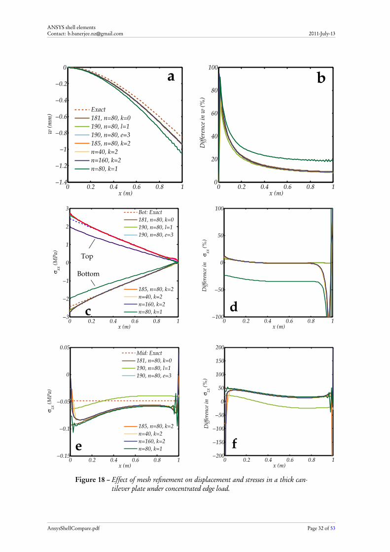
For a plate modeled with SOLID185 elements, the displacements and stresses along y = 0 areplotted in Figure 18 (p. 32). Predictions using SOLID185 elements are compared with the isotropic,“exact”, solution, SHELL181 simulations with KEYOPT(3)=0, and one-element (l = 1) and three-element (e = 3) SOLSH190 calculations. The integration schemes considered for the SOLID185element are uniform reduced integration (k = 1) and enhanced assumed strain (k = 2). Threethrough-thickness elements have been used in all the SOLID185 simulations.
The displacement plots in parts a and b of the figure show that convergence of the solutionalong y = 0 is rapid and is achieved with only 40 elements along an edge (n = 40). The outlier ingreen corresponds to a reduced integration calculation with SOLID185 elements. The light greenoutlier that becomes apparent in part b of the figure corresponds to a SOLSH190 calculation withone element through the thickness. A slightly smaller displacement is predicted by the ANSYSTM
model when this options is used.
Parts c and d of the figure show the bending stresses at the top and bottom of the plate alongy = 0. We find that the one-element SOLSH190 simulation and the SHELL181 simulation givenearly identical results. On the other hand, the three-element SOLSH190 simulation gives resultsthat are similar to those using SOLID185 elements. The increase in the number of degrees offreedom and the resulting change in the nodal boundary conditions is responsible for the lack ofsymmetry between the top and bottom stresses when more than one element is used through thethickness.
Examination of the transverse shear stress plots in parts e and f of the figure shows that reducedintegration of SOLID185 elements leads to fluctuations close to the boundaries. However, all the
AnsysShellCompare.pdf Page 29 of 53

ANSYS shell elementsContact: [email protected] 2011-July-13
0 0.2 0.4 0.6 0.8 1−1
−0.8
−0.6
−0.4
−0.2
0
x (m)
w (
mm
)
Exact
181, n=80, k=0
190, n=80, l=1
n=40
n=160
n=80, l=3
n=80, l=1, e=3
0 0.2 0.4 0.6 0.8 10
20
40
60
80
100
x (m)
Dif
fere
nce
in
w (
%)
ba
0 0.2 0.4 0.6 0.8 1−3
−2
−1
0
1
2
3
x (m)
σxx
(M
Pa)
Bot: Exact
181, n=80, k=0
190, n=80, l=1
n=40
n=160
n=80, l=3
n=80, l=1, e=3
0 0.2 0.4 0.6 0.8 1−100
−50
0
50
100
x (m)
Dif
fere
nce
in
σxx
(%
)
0 0.2 0.4 0.6 0.8 1−0.1
−0.08
−0.06
−0.04
−0.02
0
x (m)
σzx
(M
Pa)
Mid: Exact
181, n=80, k=0
190, n=80, l=1
n=40
n=160
n=80, l=3
n=80, l=1, e=3
0 0.2 0.4 0.6 0.8 1−100
−50
0
50
100
x (m)
Dif
fere
nce
in
σzx
(%
)
d
fe
c
Bottom
Top
Figure 17 – Effect of mesh refinement on displacement and stresses in a thick can-tilever plate under concentrated edge load.
AnsysShellCompare.pdf Page 30 of 53

ANSYS shell elementsContact: [email protected] 2011-July-13
SOLID185 simulations produce results that are close to those predicted by SHELL181 elements andnearly identical to those produced by SOLSH190 elements with three through-thickness elements.This indicates that SOLSH190 elements with one through-thickness element are not very accuratein predicting transverse shear stresses.
AnsysShellCompare.pdf Page 31 of 53
ANSYS shell elementsContact: [email protected] 2011-July-13
0 0.2 0.4 0.6 0.8 1−1.4
−1.2
−1
−0.8
−0.6
−0.4
−0.2
0
x (m)
w (
mm
)
Exact
181, n=80, k=0
190, n=80, l=1
190, n=80, e=3
185, n=80, k=2
n=40, k=2
n=160, k=2
n=80, k=1
0 0.2 0.4 0.6 0.8 10
20
40
60
80
100
x (m)
Dif
fere
nce
in
w (
%)
a b
0 0.2 0.4 0.6 0.8 1−3
−2
−1
0
1
2
3
x (m)
σxx
(M
Pa)
Bot: Exact
Mid: Exact
181, n=80, k=0
181, n=80, k=0
190, n=80, l=1
190, n=80, l=1
190, n=80, e=3
190, n=80, e=3
185, n=80, k=2
185, n=80, k=2
n=40, k=2
n=40, k=2
n=160, k=2
n=160, k=2
n=80, k=1
n=80, k=1
0 0.2 0.4 0.6 0.8 1−100
−50
0
50
100
x (m)
Dif
fere
nce
in
σ
xx (
%)
0 0.2 0.4 0.6 0.8 1−0.15
−0.1
−0.05
0
0.05
x (m)
σzx
(M
Pa)
0 0.2 0.4 0.6 0.8 1−200
−150
−100
−50
0
50
100
150
200
x (m)
Dif
fere
nce
in
σ
zx (
%)
c d
e f
Bottom
Top
Figure 18 – Effect of mesh refinement on displacement and stresses in a thick can-tilever plate under concentrated edge load.
AnsysShellCompare.pdf Page 32 of 53
ANSYS shell elementsContact: [email protected] 2011-July-13
6 Cantilevered isotropic sandwich plate with concentrated edge load
So far we have not truly explored the layering capabilities of ANSYSTM shell elements except toverify that layering commands had been correctly input into simulations and the correct data werebeing extracted. In this section we investigate true sandwich composites with significantly differentfacesheet/core geometries and material properties.
The sandwich panels have the same planar dimensions as before, 1 m × 1 m. Two sandwichpanel models of different layer thicknesses are explored in this section:
1. a thin panel with facesheet thickness 1/1000th the panel length (i.e., 1 mm) and core thickness1/50th the panel length (i.e., 20 mm), and
2. a thick panel with facesheet thickness 1/100th the panel length (i.e., 1 cm) and core thickness1/10th the panel length (i.e., 10 cm).
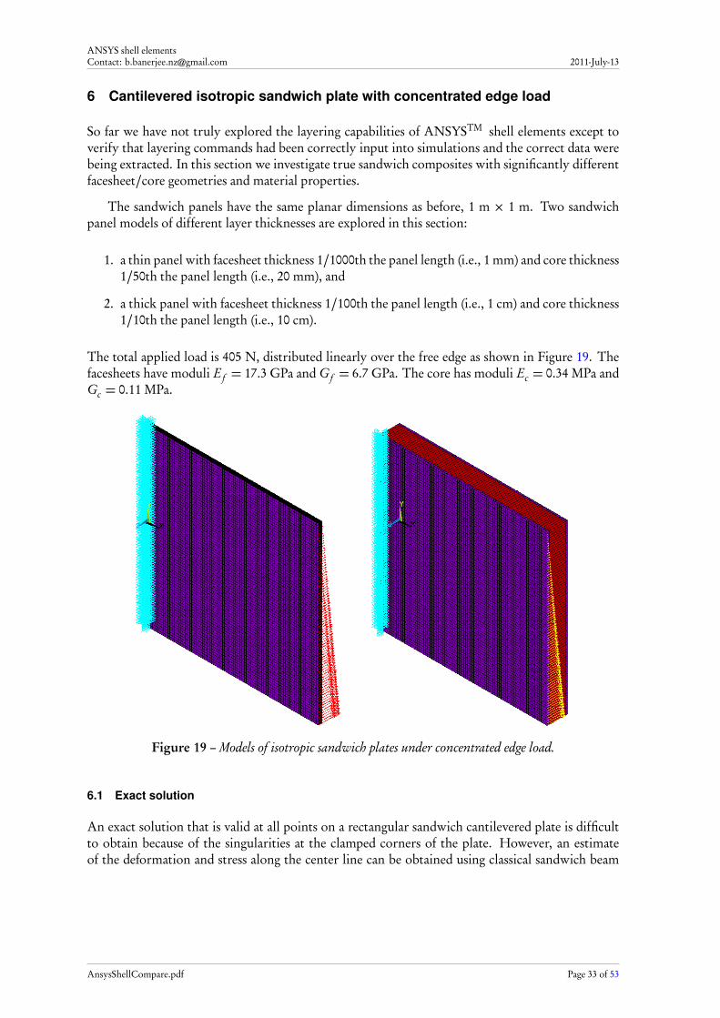
The total applied load is 405 N, distributed linearly over the free edge as shown in Figure 19. Thefacesheets have moduli E f = 17.3 GPa and G f = 6.7 GPa. The core has moduli Ec = 0.34 MPa andGc = 0.11 MPa.
Figure 19 – Models of isotropic sandwich plates under concentrated edge load.
6.1 Exact solution
An exact solution that is valid at all points on a rectangular sandwich cantilevered plate is difficultto obtain because of the singularities at the clamped corners of the plate. However, an estimateof the deformation and stress along the center line can be obtained using classical sandwich beam
AnsysShellCompare.pdf Page 33 of 53
ANSYS shell elementsContact: [email protected] 2011-July-13
theory. Following Zenkert [6] (p. 63), the solution for “thin” facesheets is w = wb +ws where
wb (x) =qa3
6D
� x
a
�2�
3−x
a
�
ws (x) =−D
S
d 3wb
d x3=
q x
S
(10)
and the bending and shear contributions to the out-of-plane displacement, respectively. In the aboveequations, q is the applied load, D is the bending stiffness of the beam, S is the shear stiffness ofthe beam, and a is the length of the beam. For a linearly distributed edge load along the edge x = a,with maximum q0 at y = −b/2 and minimum 0 at y = b/2, we have q = b q0/2 where b is thewidth of the plate. The bending and shear stiffnesses are defined as
D =f h2E f
2and S =
κh2Gc
c
where E f is the Young’s modulus of the facesheets, Gc is the shear modulus of the core, c is thethickness of the core, and h = f + c where f is the thickness of the facesheet. It is assumed thatboth facesheets have the same thickness.
The stresses are given by
σx x =−E f zd 2wb
d x2=
zqE f
D(x − a)
σz x =hGc
c
d ws
d x=
hqGc
cS
(11)
where σx x is the bending stress in the facesheets, and σz x is the shear stress in the core.
For a sandwich beam with “thick” facesheets, the solution has the form [7] (p. 13)
wb (x) =qa3
6D
� x
a
�2�
3−x
a
�
−2qD f
DS[x − f (x)]
ws (x) =q x
S+
q
S + 2S f−
q
S
!
f (x)(12)
where D f and S f are the bending and shear stiffnesses of the facesheets, defined as
D f =f 3E f
12and S f = κ f G f
where G f is the shear modulus of the beam, and
f (x) =1
α[sinh(αx)+ {1− cosh(αx)} tanh(αa)] , α=
SS f
(S + 2S f )D f
1/2
.
The corresponding stresses are
σx x =zqE f
D
�
(x − a)−2αD f
S
sinh[α(x − a)]
cosh(αa)
�
−z f qE f
S
2αS f
S + 2S f
sinh[α(x − a)]
cosh(αa)
σz x =hqGc
cS
1−2S f
S + 2S f
cosh[α(x − a)]
cosh(αa)
(13)
AnsysShellCompare.pdf Page 34 of 53
ANSYS shell elementsContact: [email protected] 2011-July-13
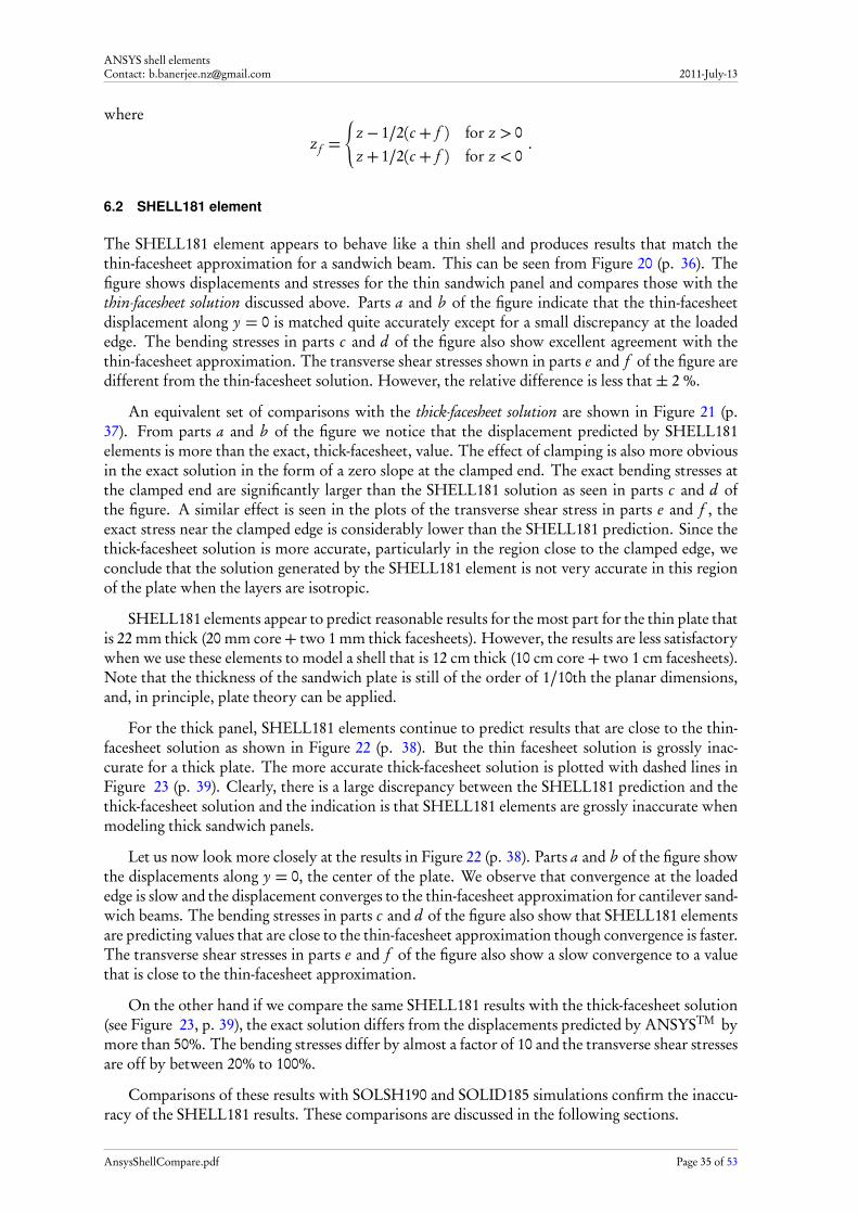
where
z f =
(
z − 1/2(c + f ) for z > 0z + 1/2(c + f ) for z < 0
.
6.2 SHELL181 element
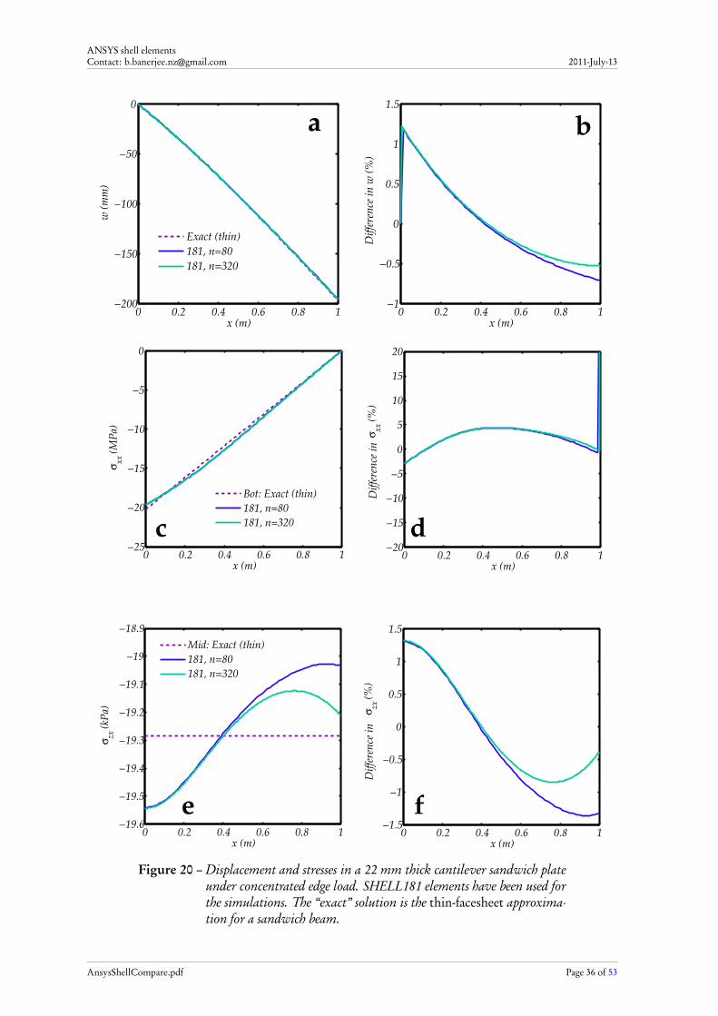
The SHELL181 element appears to behave like a thin shell and produces results that match thethin-facesheet approximation for a sandwich beam. This can be seen from Figure 20 (p. 36). Thefigure shows displacements and stresses for the thin sandwich panel and compares those with thethin-facesheet solution discussed above. Parts a and b of the figure indicate that the thin-facesheetdisplacement along y = 0 is matched quite accurately except for a small discrepancy at the loadededge. The bending stresses in parts c and d of the figure also show excellent agreement with thethin-facesheet approximation. The transverse shear stresses shown in parts e and f of the figure aredifferent from the thin-facesheet solution. However, the relative difference is less that ± 2 %.
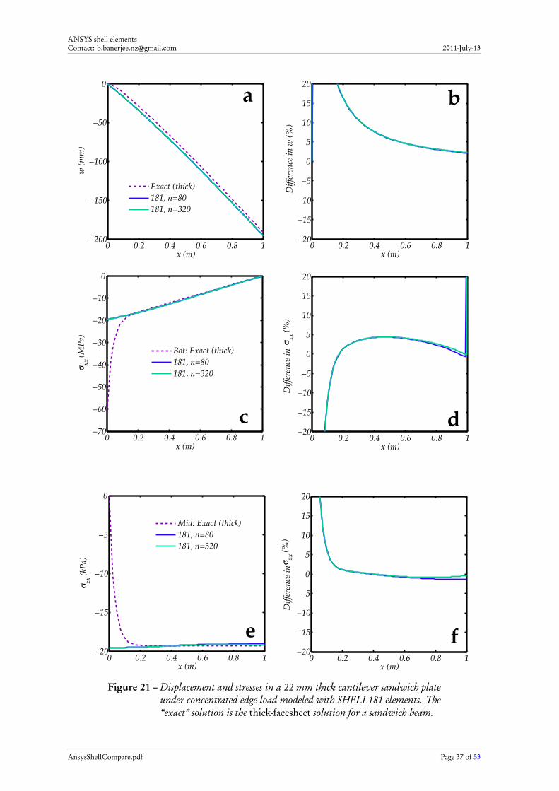
An equivalent set of comparisons with the thick-facesheet solution are shown in Figure 21 (p.37). From parts a and b of the figure we notice that the displacement predicted by SHELL181elements is more than the exact, thick-facesheet, value. The effect of clamping is also more obviousin the exact solution in the form of a zero slope at the clamped end. The exact bending stresses atthe clamped end are significantly larger than the SHELL181 solution as seen in parts c and d ofthe figure. A similar effect is seen in the plots of the transverse shear stress in parts e and f , theexact stress near the clamped edge is considerably lower than the SHELL181 prediction. Since thethick-facesheet solution is more accurate, particularly in the region close to the clamped edge, weconclude that the solution generated by the SHELL181 element is not very accurate in this regionof the plate when the layers are isotropic.
SHELL181 elements appear to predict reasonable results for the most part for the thin plate thatis 22 mm thick (20 mm core+ two 1 mm thick facesheets). However, the results are less satisfactorywhen we use these elements to model a shell that is 12 cm thick (10 cm core+ two 1 cm facesheets).Note that the thickness of the sandwich plate is still of the order of 1/10th the planar dimensions,and, in principle, plate theory can be applied.
For the thick panel, SHELL181 elements continue to predict results that are close to the thin-facesheet solution as shown in Figure 22 (p. 38). But the thin facesheet solution is grossly inac-curate for a thick plate. The more accurate thick-facesheet solution is plotted with dashed lines inFigure 23 (p. 39). Clearly, there is a large discrepancy between the SHELL181 prediction and thethick-facesheet solution and the indication is that SHELL181 elements are grossly inaccurate whenmodeling thick sandwich panels.
Let us now look more closely at the results in Figure 22 (p. 38). Parts a and b of the figure showthe displacements along y = 0, the center of the plate. We observe that convergence at the loadededge is slow and the displacement converges to the thin-facesheet approximation for cantilever sand-wich beams. The bending stresses in parts c and d of the figure also show that SHELL181 elementsare predicting values that are close to the thin-facesheet approximation though convergence is faster.The transverse shear stresses in parts e and f of the figure also show a slow convergence to a valuethat is close to the thin-facesheet approximation.
On the other hand if we compare the same SHELL181 results with the thick-facesheet solution(see Figure 23, p. 39), the exact solution differs from the displacements predicted by ANSYSTM bymore than 50%. The bending stresses differ by almost a factor of 10 and the transverse shear stressesare off by between 20% to 100%.
Comparisons of these results with SOLSH190 and SOLID185 simulations confirm the inaccu-racy of the SHELL181 results. These comparisons are discussed in the following sections.
AnsysShellCompare.pdf Page 35 of 53
ANSYS shell elementsContact: [email protected] 2011-July-13
0 0.2 0.4 0.6 0.8 1−200
−150
−100
−50
0
x (m)
w (
mm
)
Exact (thin)
181, n=80
181, n=320
0 0.2 0.4 0.6 0.8 1−1
−0.5
0
0.5
1
1.5
x (m)
Dif
fere
nce
in
w (
%)
a b
0 0.2 0.4 0.6 0.8 1−25
−20
−15
−10
−5
0
x (m)
σxx
(M
Pa)
Bot: Exact (thin)
181, n=80
181, n=320
0 0.2 0.4 0.6 0.8 1−20
−15
−10
−5
0
5
10
15
20
x (m)
Dif
fere
nce
in
σxx
(%
)
0 0.2 0.4 0.6 0.8 1−19.6
−19.5
−19.4
−19.3
−19.2
−19.1
−19
−18.9
x (m)
σzx
(kP
a)
Mid: Exact (thin)
181, n=80
181, n=320
0 0.2 0.4 0.6 0.8 1−1.5
−1
−0.5
0
0.5
1
1.5
x (m)
Dif
fere
nce
in
σ
zx (
%)
c d
e f
Figure 20 – Displacement and stresses in a 22 mm thick cantilever sandwich plateunder concentrated edge load. SHELL181 elements have been used forthe simulations. The “exact” solution is the thin-facesheet approxima-tion for a sandwich beam.
AnsysShellCompare.pdf Page 36 of 53
ANSYS shell elementsContact: [email protected] 2011-July-13
0 0.2 0.4 0.6 0.8 1−200
−150
−100
−50
0
x (m)
w (
mm
)
Exact (thick)
181, n=80
181, n=320
0 0.2 0.4 0.6 0.8 1−20
−15
−10
−5
0
5
10
15
20
x (m)
Dif
fere
nce
in
w (
%)
a b
0 0.2 0.4 0.6 0.8 1−70
−60
−50
−40
−30
−20
−10
0
x (m)
σxx
(M
Pa)
Bot: Exact (thick)
181, n=80
181, n=320
0 0.2 0.4 0.6 0.8 1−20
−15
−10
−5
0
5
10
15
20
x (m)
Dif
fere
nce
in
σxx
(%
)
0 0.2 0.4 0.6 0.8 1−20
−15
−10
−5
0
x (m)
σzx
(kP
a)
Mid: Exact (thick)
181, n=80
181, n=320
0 0.2 0.4 0.6 0.8 1−20
−15
−10
−5
0
5
10
15
20
x (m)
Dif
fere
nce
in
σzx
(%
)
e
c d
f
Figure 21 – Displacement and stresses in a 22 mm thick cantilever sandwich plateunder concentrated edge load modeled with SHELL181 elements. The“exact” solution is the thick-facesheet solution for a sandwich beam.
AnsysShellCompare.pdf Page 37 of 53

ANSYS shell elementsContact: [email protected] 2011-July-13
0 0.2 0.4 0.6 0.8 1−30
−25
−20
−15
−10
−5
0
x (m)
w (
mm
)
Exact (thin)
181, n=80, k=2
n=40
n=160
n=320
0 0.2 0.4 0.6 0.8 1−1.4
−1.2
−1
−0.8
−0.6
−0.4
−0.2
0
x (m)
Dif
fere
nce
in
w (
%)
a b
0 0.2 0.4 0.6 0.8 1−0.5
0
0.5
x (m)
σxx
(M
Pa)
Bot: Exact (thin)
181, n=80, k=2
n=40
n=160
n=320
0 0.2 0.4 0.6 0.8 1−20
0
20
40
60
80
100
120
x (m)
Dif
fere
nce
in
σ
xx (
%)
0 0.2 0.4 0.6 0.8 1−3.7
−3.68
−3.66
−3.64
−3.62
−3.6
−3.58
−3.56
x (m)
σzx
(kP
a)
Mid: Exact (thin)
181, n=80, k=2
n=40
n=160
n=320
0 0.2 0.4 0.6 0.8 1−3
−2.5
−2
−1.5
−1
−0.5
0
x (m)
Dif
fere
nce
in
σzx
(%
)
c d
e f
Bottom
Top
Figure 22 – Displacement and stresses in a 12 cm thick cantilever sandwich plateunder concentrated edge load modeled with SHELL181 elements. The“exact” solution is the thick-facesheet solution for a sandwich beam.
AnsysShellCompare.pdf Page 38 of 53
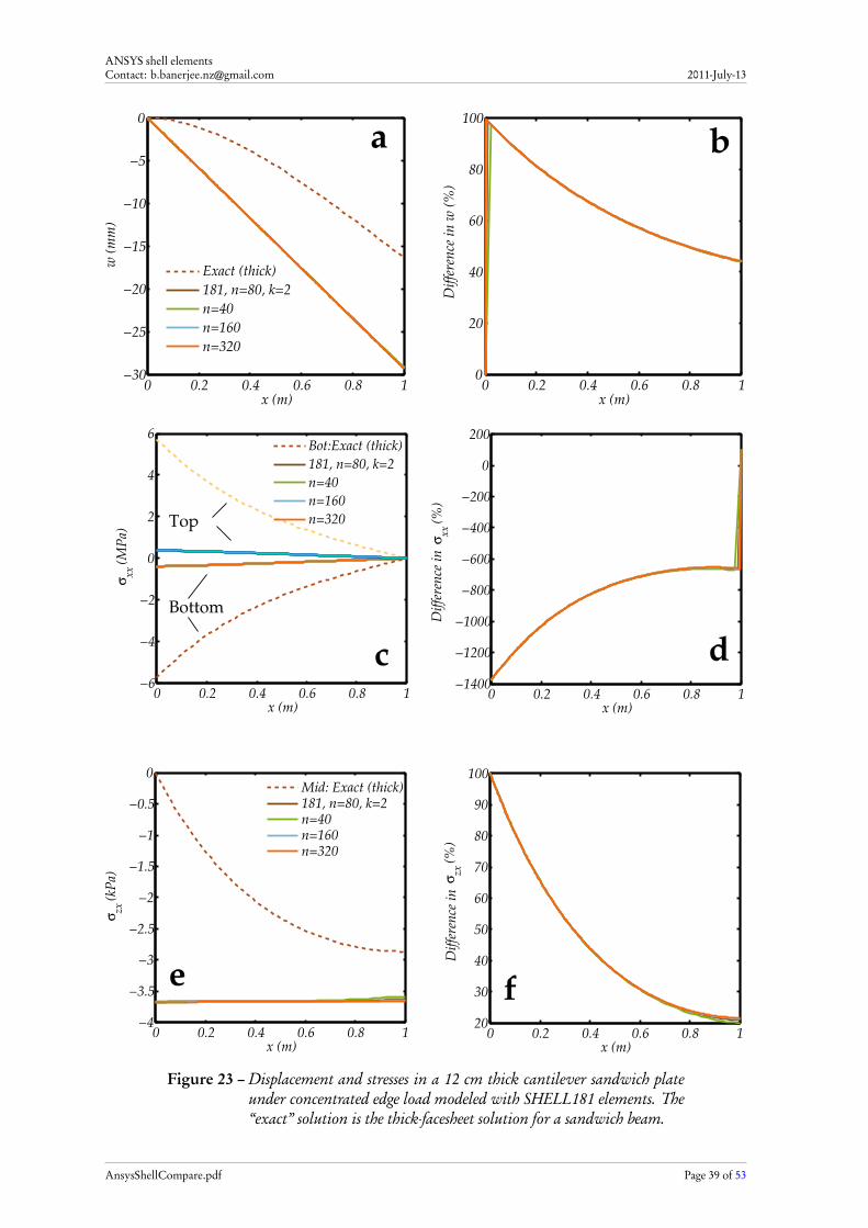
ANSYS shell elementsContact: [email protected] 2011-July-13
0 0.2 0.4 0.6 0.8 1−30
−25
−20
−15
−10
−5
0
x (m)
w (
mm
)
Exact (thick)
181, n=80, k=2
n=40
n=160
n=320
0 0.2 0.4 0.6 0.8 10
20
40
60
80
100
x (m)
Dif
fere
nce
in
w (
%)
a b
0 0.2 0.4 0.6 0.8 1−6
−4
−2
0
2
4
6
x (m)
σxx
(M
Pa)
Bot:Exact (thick)
181, n=80, k=2
n=40
n=160
n=320
0 0.2 0.4 0.6 0.8 1−1400
−1200
−1000
−800
−600
−400
−200
0
200
x (m)
Dif
fere
nce
in
σxx
(%
)
0 0.2 0.4 0.6 0.8 1−4
−3.5
−3
−2.5
−2
−1.5
−1
−0.5
0
x (m)
σzx
(kP
a)
Mid: Exact (thick)181, n=80, k=2n=40n=160n=320
0 0.2 0.4 0.6 0.8 120
30
40
50
60
70
80
90
100
x (m)
Dif
fere
nce
in
σzx
(%
)
c d
ef
Top
Bottom
Figure 23 – Displacement and stresses in a 12 cm thick cantilever sandwich plateunder concentrated edge load modeled with SHELL181 elements. The“exact” solution is the thick-facesheet solution for a sandwich beam.
AnsysShellCompare.pdf Page 39 of 53

ANSYS shell elementsContact: [email protected] 2011-July-13
6.3 SOLSH190 element
In contrast with the SHELL181 element, the SOLSH190 element behaves more like a sandwichshell with thick facesheets and matches the thick-facesheet solution quite accurately. Since thethick-facesheet solution is more accurate, we will only compare the ANSYSTM results with thatsolution. The displacement and stresses predicted by SOLSH190 elements are compared with thethick-facesheet solution and the SHELL181 solution in Figure 24 (p. 41). All SOLSH190 simula-tions except one were performed with three elements through the thickness.
Several different boundary conditions have been explored in our study. The asymmetry be-tween the bending stresses at the top and bottom of the panel (observed in isotropic and orthotropiccantilever plates) was found to be caused by the positioning the load to act only on the top surfaceof the plate. If, instead, the load was applied so that half was at the top and half at the bottom, theasymmetry disappeared. The results shown in Figure 24 have all been obtained using loads appliedboth at the top and the bottom of the plate at the loaded edge. The displacement boundary condi-tions at the clamped edge also have a strong effect on the results. Several boundary conditions havebeen explored; the results from three types of applied displacement are shown in the figure. Theseare b c = 0, where the degrees of freedom of all nodes at the clamped edge are fixed; b c = 2, whereonly nodes at the mid-planes of the facesheets and core are fixed; and b c = 4 where the top node ofthe top facesheet, the bottom node of the bottom facesheet, and the mid-plane node of the core arefixed at the clamped end.
Parts a and b of Figure 24 show the displacements predicted when SOLSH190 elements areused. The significant outlier corresponds to the case where one element is used through the thick-ness of the sandwich (e = 1). This element has three layers; the two outer layers correspond tothe facesheets and the inner layer is the core. Clearly, the element is excessively stiff and thereforeinadequate. If we now examine the SHELL181 solution in blue, we observe that it is close to theSOLSH190 with the b c = 2 option. This boundary condition poorly constrains the clamped edgeand therefore cannot be an accurate representation of a clamped boundary condition. The fact thatthe SHELL181 solution is identical to the SOLSH190 solutions with extremely compliant bound-ary conditions is further indication that these solutions cannot be accurate. Notice that the fullyclamped solution (b c = 0) and the clamped facesheet with partially clamped core (b c = 4) lead toresults that are very close to the thick-facesheet exact solution. Convergence is also rapid as seenfrom the overlapping curves for 80 elements and 320 elements along an edge.
The plots of bending stress shown in parts c and d of the figure are also further illustrativeof the accuracy of the SOLSH190 calculations. With a properly constrained clamped edge, theSOLSH190 element predicts stresses that are identical to the thick-facesheet exact value, even atthe clamped edge where the stress increases significantly. However, the SHELL181 and SOLSH190with b c = 2 predict much lower stresses at the clamped edge.
If we examine the transverse shear stresses in parts e and f of the figure, we notice that SOLSH190calculations with one element (containing three layers) through the thickness overestimate the stresssignificantly. However, with the correctly constrained clamped edge and three elements (each con-taining one layer) through-thickness, the SOLSH190 solutions are almost identical to the exact,thick-facesheet, solution. The large difference close to the clamped edge observed in part f of thefigure is due to the large gradient in the stress close to that edge. Clearly, the fact that the thick-facesheet solution is matched well by SOLSH190 elements indicates that these elements are moreaccurate than SHELL181 elements.
Similar results are observed for the thicker panel in which the thick-facesheet solution and theSOLSH190 solution are quite close as can be observed in Figure 25 (p. 43). The SOLSH190 resultsshown in the figure are from calculations with three elements through the thickness (e = 3) andwith the load applied on both the top and bottom nodes of the panel at the loaded edge (l oad = 2).
AnsysShellCompare.pdf Page 40 of 53
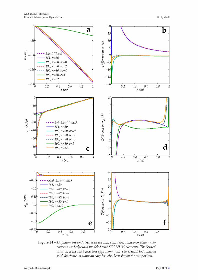
ANSYS shell elementsContact: [email protected] 2011-July-13
0 0.2 0.4 0.6 0.8 1−200
−150
−100
−50
0
x (m)
w (
mm
)
Exact (thick)
181, n=80
190, n=80, bc=0
190, n=80, bc=2
190, n=80, bc=4
190, n=80, e=1
190, n=320
0 0.2 0.4 0.6 0.8 1−20
−15
−10
−5
0
5
10
15
20
x (m)
Dif
fere
nce
in
w (
%)
a b
0 0.2 0.4 0.6 0.8 1−70
−60
−50
−40
−30
−20
−10
0
x (m)
σxx
(M
Pa)
Bot: Exact (thick)
181, n=80
190, n=80, bc=0
190, n=80, bc=2
190, n=80, bc=4
190, n=80, e=1
190, n=320
0 0.2 0.4 0.6 0.8 1−20
−15
−10
−5
0
5
10
15
20
x (m)
Dif
fere
nce
in
σxx
(%
)
0 0.2 0.4 0.6 0.8 1−0.35
−0.3
−0.25
−0.2
−0.15
−0.1
−0.05
0
x (m)
σzx
(M
Pa)
Mid: Exact (thick)
181, n=80
190, n=80, bc=0
190, n=80, bc=2
190, n=80, bc=4
190, n=80, e=1
190, n=320
0 0.2 0.4 0.6 0.8 1−20
−15
−10
−5
0
5
10
15
20
x (m)
Dif
fere
nce
in
σzx
(%
)
c d
e f
Figure 24 – Displacement and stresses in the thin cantilever sandwich plate underconcentrated edge load modeled with SOLSH190 elements. The “exact”solution is the thick-facesheet approximation. The SHELL181 solutionwith 80 elements along an edge has also been shown for comparison.
AnsysShellCompare.pdf Page 41 of 53

ANSYS shell elementsContact: [email protected] 2011-July-13
The SOLSH190 results shown in cyan are an exception in that they correspond to the situationwhere the load is applied only to the top edge of the panel (l oad = 1).
The displacements along y = 0 are shown in parts a and b of the figure. The SHELL181solution and the SOLSH190 solution with b c = 2 are identical, and certainly wrong. All the otherSOLSH190 results match the thick-facesheet exact solution well. In fact, as seen in part b of thefigure, the best match is for the case where all nodes at the clamped end are fixed (b c = 0).
If we examine the bending stresses in parts c and d of the figure, we once again see that theSOLSH190 simulation with fully clamped nodes (b c = 0), and loaded both on the top and thebottom (l oad = 2), matches the exact thick-facesheet solution best. The stresses predicted bySHELL181 elements (and SOLSH190 with b c = 2) are far too low. A partially clamped core,b c = 4, shows large fluctuations near the clamped edge and a top loaded plate (190, n = 80, e = 3)shows an asymmetry between the top and bottom facesheets (note that the top facesheet solutionsare not shown in the plots).
The transverse shear stress solutions in parts e and f of the figure show similar trends. Thel oad = 2, b c = 0 case matches the exact solution perfectly except in a region close to the clampededge. The discrepancy has been tracked down to the way in which ANSYSTM interpolates resultsto a PATH when the PDEF command is used with the NOAVG option.
These results further confirm the accuracy of SOLSH190 elements relative to SHELL181 ele-ments.
6.4 SOLID185 element
The exact solution can be checked by modeling the plate with three-dimensional SOLID185 ele-ments and comparing the results. Figure 26 (p. 44) shows one such set of comparisons. In the figure,SOLID185 simulations with clamped mid-planes only (b c = 2) and fully clamped facesheets(b c =4) are compared with the thick-facesheet exact solution, the SHELL181 solution, and SOLSH190solutions with partially or fully clamped facesheets (b c = 2 or b c = 4). In the SOLID185 cal-culations each facesheet has been modeled with four through-thickness elements and the core has20 through-thickness elements. Also, the SOLID185 calculations use the enhanced assumed strainelement formulation.
The displacement solution and the difference between ANSYSTM results and the exact (thick-facesheet) solutions are plotted in parts a and b of the figure. When only the mid-planes of thefacesheets and core are clamped, the SOLID185, SOLSH190, and SHELL181 solutions are identi-cal and match the thin-facesheet solution. On the other hand, when the facesheets are clamped,though the SOLID185 and SOLSH190 solutions are identical, they are closer to the more accuratethick-facesheet solution. These results indicate that SOLID185 and SOLSH190 elements behaveidentically and, with the correct boundary conditions, are more accurate than SHELL181 elements.
Parts c and d of the figure show the bending stresses at the bottom of the sandwich plate. Onceagain, we see that SOLID185 and SOLSH190 elements behave identically and, when appropriatelyclamped, match the exact solution very well. The same behavior is seen in parts e and f of thefigure which depict the transverse shear stresses at the mid-surface of the plate along y = 0. Theseresults confirm that SOLSH190 elements are superior to SHELL181 elements for modeling sand-wich panels with isotropic facesheets and cores.
AnsysShellCompare.pdf Page 42 of 53
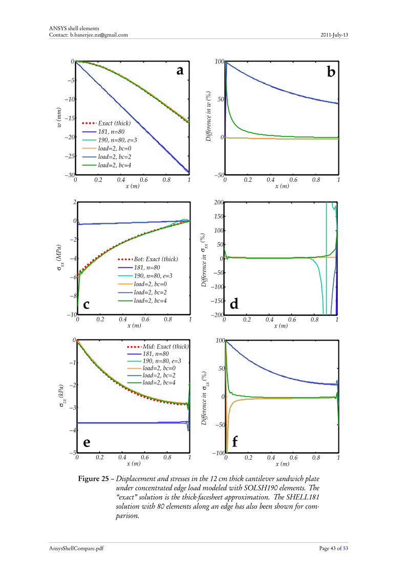
ANSYS shell elementsContact: [email protected] 2011-July-13
0 0.2 0.4 0.6 0.8 1−30
−25
−20
−15
−10
−5
0
x (m)
w (
mm
)
Exact (thick)
181, n=80
190, n=80, e=3
load=2, bc=0
load=2, bc=2
load=2, bc=4
0 0.2 0.4 0.6 0.8 1−50
0
50
100
x (m)
Dif
fere
nce
in
w (
%)
ba
0 0.2 0.4 0.6 0.8 1−10
−8
−6
−4
−2
0
2
x (m)
σxx
(M
Pa)
Bot: Exact (thick)
181, n=80
190, n=80, e=3
load=2, bc=0
load=2, bc=2
load=2, bc=4
0 0.2 0.4 0.6 0.8 1−200
−150
−100
−50
0
50
100
150
200
x (m)
Dif
fere
nce
in
σxx
(%
)
0 0.2 0.4 0.6 0.8 1−5
−4
−3
−2
−1
0
x (m)
σzx
(kP
a)
Mid: Exact (thick)181, n=80190, n=80, e=3load=2, bc=0load=2, bc=2load=2, bc=4
0 0.2 0.4 0.6 0.8 1−100
−50
0
50
100
x (m)
Dif
fere
nce
in
σzx
(%
)
c d
e f
Figure 25 – Displacement and stresses in the 12 cm thick cantilever sandwich plateunder concentrated edge load modeled with SOLSH190 elements. The“exact” solution is the thick-facesheet approximation. The SHELL181solution with 80 elements along an edge has also been shown for com-parison.
AnsysShellCompare.pdf Page 43 of 53
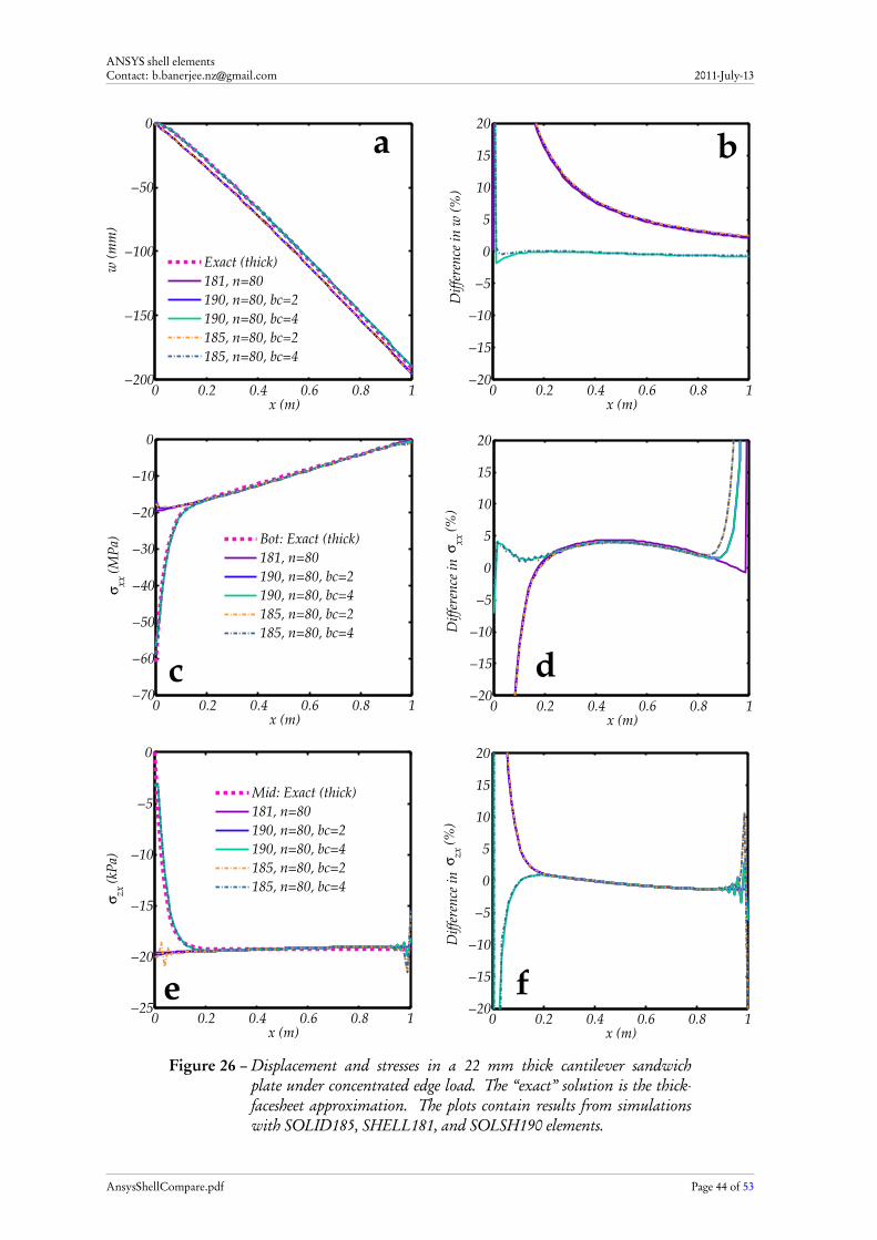
ANSYS shell elementsContact: [email protected] 2011-July-13
0 0.2 0.4 0.6 0.8 1−200
−150
−100
−50
0
x (m)
w (
mm
)
Exact (thick)
181, n=80
190, n=80, bc=2
190, n=80, bc=4
185, n=80, bc=2
185, n=80, bc=4
0 0.2 0.4 0.6 0.8 1−20
−15
−10
−5
0
5
10
15
20
x (m)
Dif
fere
nce
in
w (
%)
a b
0 0.2 0.4 0.6 0.8 1−70
−60
−50
−40
−30
−20
−10
0
x (m)
σxx
(M
Pa) Bot: Exact (thick)
181, n=80
190, n=80, bc=2
190, n=80, bc=4
185, n=80, bc=2
185, n=80, bc=4
0 0.2 0.4 0.6 0.8 1−20
−15
−10
−5
0
5
10
15
20
x (m)
Dif
fere
nce
in
σxx
(%
)
0 0.2 0.4 0.6 0.8 1−25
−20
−15
−10
−5
0
x (m)
σzx
(kP
a)
Mid: Exact (thick)
181, n=80
190, n=80, bc=2
190, n=80, bc=4
185, n=80, bc=2
185, n=80, bc=4
0 0.2 0.4 0.6 0.8 1−20
−15
−10
−5
0
5
10
15
20
x (m)
Dif
fere
nce
in
σzx
(%
)
c d
e f
Figure 26 – Displacement and stresses in a 22 mm thick cantilever sandwichplate under concentrated edge load. The “exact” solution is the thick-facesheet approximation. The plots contain results from simulationswith SOLID185, SHELL181, and SOLSH190 elements.
AnsysShellCompare.pdf Page 44 of 53
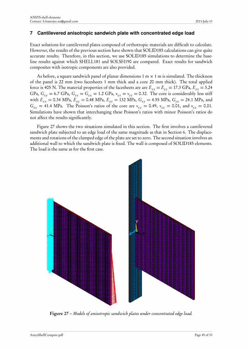
ANSYS shell elementsContact: [email protected] 2011-July-13
7 Cantilevered anisotropic sandwich plate with concentrated edge load
Exact solutions for cantilevered plates composed of orthotropic materials are difficult to calculate.However, the results of the previous section have shown that SOLID185 calculations can give quiteaccurate results. Therefore, in this section, we use SOLID185 simulations to determine the base-line results against which SHELL181 and SOLSH190 are compared. Exact results for sandwichcomposites with isotropic components are also provided.
As before, a square sandwich panel of planar dimensions 1 m× 1 m is simulated. The thicknessof the panel is 22 mm (two facesheets 1 mm thick and a core 20 mm thick). The total appliedforce is 405 N. The material properties of the facesheets are are Ex x = Eyy = 17.3 GPa, Ez z = 3.24GPa, Gxy = 6.7 GPa, Gy z = Gz x = 1.2 GPa, νx z = νy z = 0.32. The core is considerably less stiffwith Ex x = 0.34 MPa, Eyy = 0.48 MPa, Ez z = 132 MPa, Gxy = 4.55 MPa, Gy z = 24.1 MPa, andGz x = 41.4 MPa. The Poisson’s ratios of the core are νxy = 0.49, νx z = 0.01, and νy z = 0.01.Simulations have shown that interchanging these Poisson’s ratios with minor Poisson’s ratios donot affect the results significantly.
Figure 27 shows the two situations simulated in this section. The first involves a cantileveredsandwich plate subjected to an edge load of the same magnitude as that in Section 6. The displace-ments and rotations of the clamped edge of the plate are set to zero. The second situation involves anadditional wall to which the sandwich plate is fixed. The wall is composed of SOLID185 elements.The load is the same as for the first case.
Figure 27 – Models of anisotropic sandwich plates under concentrated edge load.
AnsysShellCompare.pdf Page 45 of 53
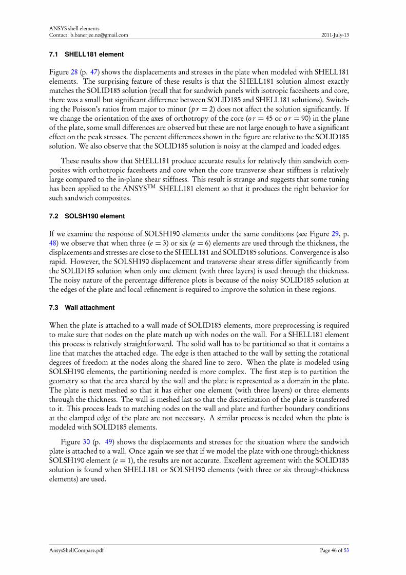
ANSYS shell elementsContact: [email protected] 2011-July-13
7.1 SHELL181 element
Figure 28 (p. 47) shows the displacements and stresses in the plate when modeled with SHELL181elements. The surprising feature of these results is that the SHELL181 solution almost exactlymatches the SOLID185 solution (recall that for sandwich panels with isotropic facesheets and core,there was a small but significant difference between SOLID185 and SHELL181 solutions). Switch-ing the Poisson’s ratios from major to minor ( p r = 2) does not affect the solution significantly. Ifwe change the orientation of the axes of orthotropy of the core (o r = 45 or o r = 90) in the planeof the plate, some small differences are observed but these are not large enough to have a significanteffect on the peak stresses. The percent differences shown in the figure are relative to the SOLID185solution. We also observe that the SOLID185 solution is noisy at the clamped and loaded edges.
These results show that SHELL181 produce accurate results for relatively thin sandwich com-posites with orthotropic facesheets and core when the core transverse shear stiffness is relativelylarge compared to the in-plane shear stiffness. This result is strange and suggests that some tuninghas been applied to the ANSYSTM SHELL181 element so that it produces the right behavior forsuch sandwich composites.
7.2 SOLSH190 element
If we examine the response of SOLSH190 elements under the same conditions (see Figure 29, p.48) we observe that when three (e = 3) or six (e = 6) elements are used through the thickness, thedisplacements and stresses are close to the SHELL181 and SOLID185 solutions. Convergence is alsorapid. However, the SOLSH190 displacement and transverse shear stress differ significantly fromthe SOLID185 solution when only one element (with three layers) is used through the thickness.The noisy nature of the percentage difference plots is because of the noisy SOLID185 solution atthe edges of the plate and local refinement is required to improve the solution in these regions.
7.3 Wall attachment
When the plate is attached to a wall made of SOLID185 elements, more preprocessing is requiredto make sure that nodes on the plate match up with nodes on the wall. For a SHELL181 elementthis process is relatively straightforward. The solid wall has to be partitioned so that it contains aline that matches the attached edge. The edge is then attached to the wall by setting the rotationaldegrees of freedom at the nodes along the shared line to zero. When the plate is modeled usingSOLSH190 elements, the partitioning needed is more complex. The first step is to partition thegeometry so that the area shared by the wall and the plate is represented as a domain in the plate.The plate is next meshed so that it has either one element (with three layers) or three elementsthrough the thickness. The wall is meshed last so that the discretization of the plate is transferredto it. This process leads to matching nodes on the wall and plate and further boundary conditionsat the clamped edge of the plate are not necessary. A similar process is needed when the plate ismodeled with SOLID185 elements.
Figure 30 (p. 49) shows the displacements and stresses for the situation where the sandwichplate is attached to a wall. Once again we see that if we model the plate with one through-thicknessSOLSH190 element (e = 1), the results are not accurate. Excellent agreement with the SOLID185solution is found when SHELL181 or SOLSH190 elements (with three or six through-thicknesselements) are used.
AnsysShellCompare.pdf Page 46 of 53
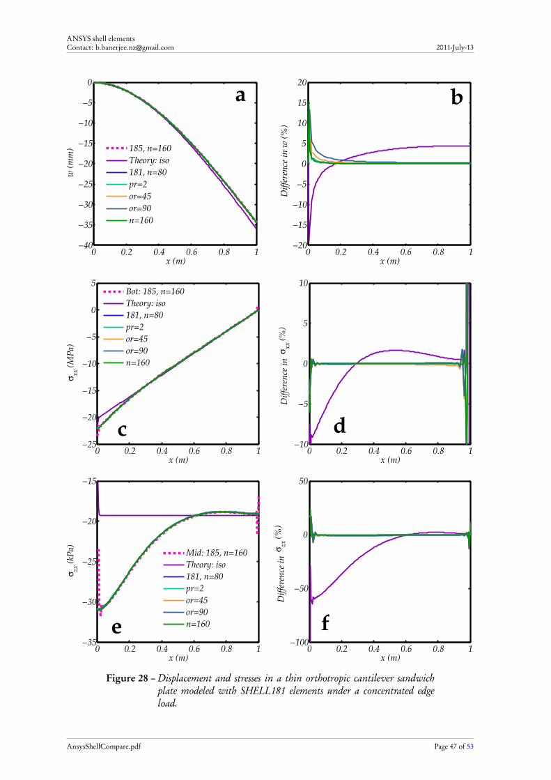
ANSYS shell elementsContact: [email protected] 2011-July-13
0 0.2 0.4 0.6 0.8 1−40
−35
−30
−25
−20
−15
−10
−5
0
x (m)
w (
mm
) 185, n=160
Theory: iso
181, n=80
pr=2
or=45
or=90
n=160
0 0.2 0.4 0.6 0.8 1−20
−15
−10
−5
0
5
10
15
20
x (m)
Dif
fere
nce
in
w (
%)
a b
0 0.2 0.4 0.6 0.8 1−25
−20
−15
−10
−5
0
5
x (m)
σxx
(M
Pa)
Bot: 185, n=160
Theory: iso
181, n=80
pr=2
or=45
or=90
n=160
0 0.2 0.4 0.6 0.8 1−10
−5
0
5
10
x (m)
Dif
fere
nce
in
σxx
(%
)
0 0.2 0.4 0.6 0.8 1−35
−30
−25
−20
−15
x (m)
σzx
(kP
a) Mid: 185, n=160
Theory: iso
181, n=80
pr=2
or=45
or=90
n=160
0 0.2 0.4 0.6 0.8 1−100
−50
0
50
x (m)
Dif
fere
nce
in
σzx
(%
)
c d
e f
Figure 28 – Displacement and stresses in a thin orthotropic cantilever sandwichplate modeled with SHELL181 elements under a concentrated edgeload.
AnsysShellCompare.pdf Page 47 of 53
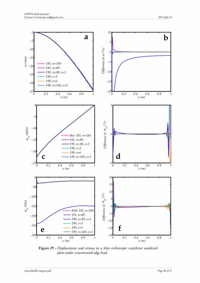
ANSYS shell elementsContact: [email protected] 2011-July-13
0 0.2 0.4 0.6 0.8 1−35
−30
−25
−20
−15
−10
−5
0
x (m)
w (
mm
)
185, n=160
181, n=80
190, n=80, e=1
190, e=3
190, e=6
190, n=160, e=3
0 0.2 0.4 0.6 0.8 1−20
−15
−10
−5
0
5
10
x (m)
Dif
fere
nce
in
w (
%)
a b
0 0.2 0.4 0.6 0.8 1−25
−20
−15
−10
−5
0
x (m)
σxx
(M
Pa)
Bot: 185, n=160
181, n=80
190, n=80, e=1
190, e=3
190, e=6
190, n=160, e=3
0 0.2 0.4 0.6 0.8 1−5
0
5
x (m)
Dif
fere
nce
in
σxx
(%
)
0 0.2 0.4 0.6 0.8 1−300
−250
−200
−150
−100
−50
0
x (m)
σzx
(kP
a)
Mid: 185, n=160
181, n=80
190, n=80, e=1
190, e=3
190, e=6
190, n=160, e=3
0 0.2 0.4 0.6 0.8 1−20
−15
−10
−5
0
5
10
15
20
x (m)
Dif
fere
nce
in
σzx
(%
)
c d
e f
Figure 29 – Displacement and stresses in a thin orthotropic cantilever sandwichplate under concentrated edge load.
AnsysShellCompare.pdf Page 48 of 53
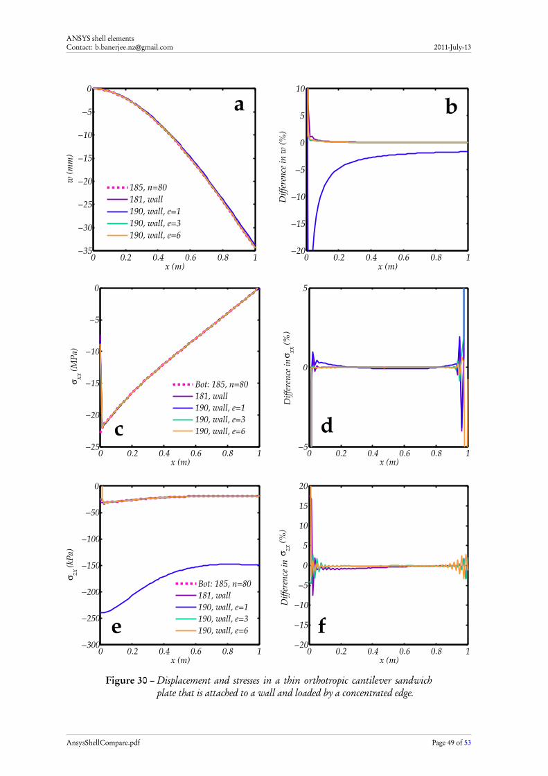
ANSYS shell elementsContact: [email protected] 2011-July-13
0 0.2 0.4 0.6 0.8 1−35
−30
−25
−20
−15
−10
−5
0
x (m)
w (
mm
)
185, n=80
181, wall
190, wall, e=1
190, wall, e=3
190, wall, e=6
0 0.2 0.4 0.6 0.8 1−20
−15
−10
−5
0
5
10
x (m)
Dif
fere
nce
in
w (
%)
a b
0 0.2 0.4 0.6 0.8 1−25
−20
−15
−10
−5
0
x (m)
σxx
(M
Pa)
Bot: 185, n=80
181, wall
190, wall, e=1
190, wall, e=3
190, wall, e=6
0 0.2 0.4 0.6 0.8 1−5
0
5
x (m)
Dif
fere
nce
in
σxx
(%
)
0 0.2 0.4 0.6 0.8 1−300
−250
−200
−150
−100
−50
0
x (m)
σzx
(kP
a)
Bot: 185, n=80
181, wall
190, wall, e=1
190, wall, e=3
190, wall, e=6
0 0.2 0.4 0.6 0.8 1−20
−15
−10
−5
0
5
10
15
20
x (m)
Dif
fere
nce
in
σzx
(%
)
c d
e f
Figure 30 – Displacement and stresses in a thin orthotropic cantilever sandwichplate that is attached to a wall and loaded by a concentrated edge.
AnsysShellCompare.pdf Page 49 of 53
ANSYS shell elementsContact: [email protected] 2011-July-13
8 Cantilevered anisotropic sandwich plate under acceleration load
Another situation of interest is when a cantilevered anisotropic plate is loaded by a body force dueto a downward acceleration of 9g . The plate has dimensions and material properties identical tothose used in the previous section. Plates modeled with SOLSH190 and SOLID185 elements wereclamped by fixing the displacements of all nodes along the clamped edge to zero. Figure 31 (p. 51)shows the displacement and stresses in the plate when different element types are used.
The displacements plotted in parts a and b of the figure are nearly identical when SOLID185,SHELL181, and SOLSH190 elements (with three through-thickness elements) are used. The outlierin light green is for the case where SOLSH190 elements were used with one element through thethickness and three layers in each element.
The bending stresses in parts c and d of the figure differ slightly from the SOLID185 solutionat the free edge. The closest solution is obtained when SOLSH190 elements with three through-thickness elements are used. The same behavior is observed in the transverse shear plots shown inparts e and f of the figure.
It can be concluded that SHELL181 elements and SOLSH190 elements both give reasonableresults when an accleration-based body force is applied.
AnsysShellCompare.pdf Page 50 of 53
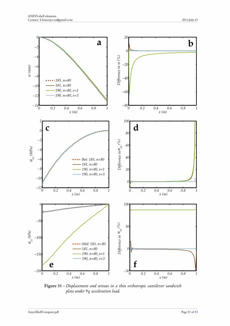
ANSYS shell elementsContact: [email protected] 2011-July-13
0 0.2 0.4 0.6 0.8 1−14
−12
−10
−8
−6
−4
−2
0
x (m)
w (
mm
)
185, n=80
181, n=80
190, n=80, e=1
190, n=80, e=3
0 0.2 0.4 0.6 0.8 1−80
−60
−40
−20
0
20
x (m)
Dif
fere
nce
in
w (
%)
a b
0 0.2 0.4 0.6 0.8 1−12
−10
−8
−6
−4
−2
0
2
x (m)
σxx
(M
Pa)
Bot: 185, n=80
181, n=80
190, n=80, e=1
190, n=80, e=3
0 0.2 0.4 0.6 0.8 1
0
20
40
60
80
100
x (m)
Dif
fere
nce
in
σxx
(%
)
0 0.2 0.4 0.6 0.8 1−200
−150
−100
−50
0
x (m)
σzx
(kP
a)
Mid: 185, n=80
181, n=80
190, n=80, e=1
190, n=80, e=3
0 0.2 0.4 0.6 0.8 1−50
0
50
100
x (m)
Dif
fere
nce
in
σzx
(%
)
c d
e f
Figure 31 – Displacement and stresses in a thin orthotropic cantilever sandwichplate under 9g acceleration load.
AnsysShellCompare.pdf Page 51 of 53
ANSYS shell elementsContact: [email protected] 2011-July-13
9 Summary
Several situations have been examined in this study with variations in plate geometry, boundaryconditions, and material properties. The following summarizes the findings of the study.
• Both SHELL181 and SOLSH190 elements appear to be more compliant that expected fromthin plate theory for isotropic plates. Plates that have a thickness that is 1/25 the planardimensions appear to be too thick for Kirchhoff-Love theory to be applicable.
• Convergence is rapid and around 80 elements per meter seems to be sufficient for a 1 m ×1 m plate that is 1/25 m thick. This number can be used as a rule of thumb for other platesizes.
• The number of integration points through the thickness does not appear to affect the solutionas long as the number is three or greater.
• The choice of KEYOPT(3) in SHELL181 elements does not affect the results in any of theloading scenarios examined in this study.
• At least three SOLSH190 elements should be used through the thickness for accurate results.A single element with three layers in not adequate for most situations. This is problematicbecause certain versions of ANSYS WorkbenchTM appear not to allow three adjacent layersif SOLSH190 elements.
• Simulations of thin structures with SOLID185 elements should use the enhanced strain op-tion (KEYOPT(2)=2) and, at least three elements through the thickness of each componentin a sandwich structure, to avoid locking behavior and for accurate results.
• Loads and displacements have to be applied on both sets of nodes in SOLSH190 elements(i.e., nodes on the top and bottom of the mid-surface) to achieve behavior that is identical tothat of SHELL181 elements.
• Care should be taken when using SHELL181 elements to model sandwich composites withisotropic core/facesheet. To check that the correct results are being obtained, a few compar-isons with SOLID185 elements with enhanced strain should be completed.
• Both SHELL181 and SOLSH190 elements perform adequately for sandwich composites withmaterial properties and geometries similar to those used in the aerospace industry, providedcare is taken to apply the correct boundary conditions when using SOLSH190 elements.
Acknowledgments
This work has been supported by The Foundation for Research Science and Technology of NewZealand through Grant UOAX0710. We would also like to acknowledge the review of the reportby Jeremy Chen, Anjukan Kathirgamanathan, and Raj Das from the University of Auckland.
References
[1] S. Timoshenko and S. Woinowsky-Krieger. Theory of plates and shells. McGraw-Hill, NewYork, 1959. 5, 16
[2] R. D. Mindlin. Influence of rotatory inertia and shear on flexural motions of isotropic, elasticplates. ASME Journal of Applied Mechanics, 18:31–38, 1951. 5
AnsysShellCompare.pdf Page 52 of 53

ANSYS shell elementsContact: [email protected] 2011-July-13
[3] C. M. Wang, G. T. Lim, J. N. Reddy, and K. H. Lee. Relationships between bending solutionsof reissner and mindlin plate theories. Engineering Structures, 23:838–849, 2001. 5
[4] G. T. Lim and J. N. Reddy. On canonical bending relationships for plates. International Journalof Solids and Structures, 40:3039–3067, 2003. 5
[5] E. Reissner and M. Stein. Torsion and transverse bending of cantilever plates. Technical Note2369, National Advisory Committee for Aeronautics, Washington, 1951. 21
[6] D. Zenkert. An Introduction to Sandwich Construction. EMAS, London, 1995. 34
[7] F. J. Plantema. Sandwich Construction. John Wiley and Sons, New York, 1966. 34
AnsysShellCompare.pdf Page 53 of 53