comparison between satellite-based and cosmic ray …
TRANSCRIPT
COMPARISON BETWEEN SATELLITE-BASED AND COSMIC RAY PROBE SOIL MOISTURE ESTIMATES: A
CASE STUDY IN THE CATHEDRAL PEAK CATCHMENT
THIGESH VATHER
Submitted in partial fulfilment of the requirements for the degree of MSc in Hydrology
School of Agriculture, Earth and Environmental Sciences
University of KwaZulu-Natal
Pietermaritzburg
Supervisor: Ms K T Chetty
Co-supervisors: Dr M G Mengistu Prof C S Everson
November 2015
i
ABSTRACT
Soil moisture is an important hydrological parameter, which is essential for a variety of
applications, extending to numerous disciplines. Currently, there are three methods of
estimating soil moisture. These include: (a) ground-based (in-situ) measurements, which are
carried out using field instruments; (b) remote sensing based methods, which use specialized
sensors on satellites and aircrafts and (c) land surface models, which use meteorological data
as inputs, at a predefined spatial resolution (Albergel et al. (2012); Mecklenburg et al., 2013).
In recent years the cosmic ray probe (CRP), which is an in-situ technique, has been
implemented in several countries across the globe. The CRP provides area-averaged soil
moisture at an intermediate scale and thus bridges the gap between in-situ point
measurements and satellite-based soil moisture estimates (Zreda et al., 2012). The aim of this
study was to first evaluate the current techniques for soil moisture estimation, in order to
identify the research gaps and limitations. The key objectives of this study were to test the
suitability of the CRP to provide spatial estimates of soil moisture and use these estimates to
validate satellite-based (remote sensing and modelled) soil moisture estimates in the
Cathedral Peak Catchment VI. The CRP was set-up and calibrated in Cathedral Peak
Catchment VI. An in-situ soil moisture network was created in Catchment VI, which was
used to validate the calibrated CRP soil moisture estimates. Once calibrated, the CRP was
found to provide spatial estimates of soil moisture, which correlated well with the in-situ soil
moisture network dataset and yielded a R2 value of 0.8445. The calibrated CRP was used to
validate satellite-based soil moisture products. The remote sensing products used were the
Level Three AMSR2 and SMOS products. The AMSR2 and SMOS products generally
under-estimated soil moisture throughout, but followed the general trend of the CRP, with
AMSR obtaining a R2 of 0.505 and SMOS obtaining a R2 of 0.4853, when compared against
the CRP estimates. The CRP was used to validate modelled soil moisture products, which
consisted of the SAHG product and the back-calculation of soil moisture, using equations by
Su et al. (2003) and Scott et al. (2003), and products derived from the SEBS Model. The
SAHG Model performed well, as it provided estimates that correlated well with the CRP
dataset and yielded a R2 value of 0.624 compared to the CRP estimates. The SEBS back-
calculation technique performed very poorly, as it over-estimated in the wet periods and
under-estimated in the dry periods.

ii
DECLARATION
I, Thigesh Vather, declare that:
(i) the research reported in this dissertation, except where otherwise indicated, is my
original work.
(ii) this dissertation has not been submitted for any degree or examination at any other
university.
(iii) this dissertation does not contain other persons’ data, pictures, graphs or other
information, unless specifically acknowledged as being sourced from other persons.
(iv) this dissertation does not contain other persons’ writing, unless specifically
acknowledged as being sourced from other researchers. Where other written sources
have been quoted, then:
(a) their words have been re-written, but the general information attributed to them
has been referenced;
(b) where their exact words have been used, their writing has been placed inside
quotation marks, and referenced.
(v) Where I have reproduced a publication of which I am an author, co-author or editor, I
have indicated, in detail, which part of the publication was actually written by myself
alone and have fully referenced such publications.
(vi) This dissertation does not contain text, graphics or tables copied and pasted from the
Internet, unless specifically acknowledged, and the source being detailed in the
Dissertation and in the References sections.
Signed: ………………..
Thigesh Vather
Supervisor: …………………………..
Miss Kershani Tinisha Chetty
Co-supervisor: …………………………
Dr Michael Mengistu

iii
PREFACE
The work undertaken and described in this dissertation was carried out in the Centre for
Water Resources Research (CWRR), in the School of Agriculture, Earth and Environmental
Science. This school is within the University of KwaZulu-Natal, Pietermaritzburg. The
following dissertation was supervised by Ms KT Chetty, Dr MG Mengistu and Prof CS
Everson.
This dissertation is original, unpublished, independent work by the author Thigesh Vather.
The work of other authors, when used, has been given the appropriate credit.

iv
ACKNOWLEDGEMENTS
The following Masters Research titled “Comparison Between Satellite-Based and Cosmic
Ray Probe Soil Moisture Estimates: A Case Study in the Cathedral Peak Catchment’’ has
been funded by the Centre for Water Resources Research (CWRR) and the National Research
Foundation (NRF). I am grateful for the aforementioned institutions for the funding they have
contributed towards this research. I would also like to acknowledge the following people and
institutions for their fundamental role in the completion of this research project:
First and foremost, I would like to thank my parents and sisters for their continuous love and
support. I appreciate all that you have done for me, not only during the past two years, but
throughout my life Thank you to my extended family and friends for all the love and support
you have given me. Thank you to Vadinie Moodley, for all the love and support, as well as
keeping me focused throughout my Masters.
Miss KT Chetty (supervisor). Thank you for your guidance and support throughout
the duration of the research project. Your mentorship has been of much value to the
completion of the dissertation.
Dr MG Mengistu (co-supervisor). Thank you for all the support and mentorship. Your
contribution towards the completion of this research study has been invaluable. Thank
you for all the field trips to Cathedral Peak and assisting me will all the aspects of my
project, such as the setting up of the cosmic ray probe, setting up of the soil moisture
network, calibrating the cosmic ray probe, teaching me how to set-up and run the
SEBS model and for assisting with any problems that arose.
Prof CS Everson (co-supervisor). Thank you for all the support and mentorship
throughout the project. Thank you for making this research project possible by
obtaining the cosmic ray probe. Thank you for all the well organized and productive
field visits. Thank you for assisting me with the various fieldwork activities that were
carried out. Thank you for organizing the various instrumentation and support
throughout the project.

v
Mrs S Rees. Thank you for assisting me with the editing of the dissertation. I really
appreciate the time and effort that you have put into improving the dissertation.
Mr S Mfeka and Mr C Pretorius. Thank you for all the assistance in the field and the
laboratory. Thank you for always being willing to help and always approachable.
The winter school. Thank you for assisting me with the first calibration, which was
the most labour intensive and time consuming calibration. I appreciate all the work
and effort that was made.
Prof TE Franz. Thank you for assisting me with the third calibration, as well as
teaching me the cosmic ray probe calibration procedure.
Dr S Sinclair. Thank you for the assistance in providing the PyTOPKAPI soil
moisture product.
Mr S Gokool. Thank you for your assistance and advice throughout the duration of
the project. Your suggestions towards improving the project were greatly beneficial
and appreciated.
Mr B Scott-Shaw. Thank you for assisting with the fire breaks.
Mrs S van Rensburg. Thank you for organizing the accommodation and other aspects
of the field trip. The work and effort that you have contributed is greatly appreciated.
Thank you to the Staff and Students of the Hydrology Department for all the help and
continuous support.

vi
TABLE OF CONTENTS Page
ABSTRACT ................................................................................................................................ i
PREFACE ................................................................................................................................. iii
ACKNOWLEDGEMENTS ...................................................................................................... iv
LIST OF TABLES .................................................................................................................... ix
LIST OF FIGURES ....................................................................................................................x
LIST OF SYMBOLS .............................................................................................................. xvi
LIST OF ABBREVIATIONS ................................................................................................. xix
1. INTRODUCTION ..............................................................................................................1
2. IN-SITU METHODS OF SOIL MOISTURE MEASUREMENT .....................................4
2.1 Conventional Methods of Soil Moisture Estimation ..................................................4
2.2 Cosmic Ray Probe ......................................................................................................6
Production of cosmic ray neutrons ...................................................................7
Moderation of neutrons ....................................................................................8
Cosmic ray probe measurements ......................................................................8
Measurement footprint and depth of the cosmic ray probe ..............................9
Advantages of the cosmic ray probe method .................................................11
3. REMOTE SENSING OF SOIL MOISTURE ...................................................................14
3.1 Overview of Remote Sensing of Soil Moisture ........................................................14
3.2 AMSR2 .....................................................................................................................15
3.3 SMOS ........................................................................................................................17

vii
3.4 Downscaling Techniques ..........................................................................................21
4. METHODS OF MODELLING SOIL MOISTURE .........................................................25
4.1 Land Surface Model (PyTOPKAPI) .........................................................................25
4.2 Surface Energy Balance System (SEBS) ..................................................................29
5. SYNTHESIS OF LITERATURE .....................................................................................34
6. METHODOLOGY ...........................................................................................................36
6.1 Study Site ..................................................................................................................37
6.2 Cosmic Ray Probe ....................................................................................................39
Set up of the cosmic ray probe .......................................................................39
Field sampling ................................................................................................42
Gravimetric water content determination .......................................................42
Creating a soil moisture network ....................................................................43
Catchment burning .........................................................................................44
Bulk density determination ............................................................................46
6.3 Calibration ................................................................................................................48
6.4 Creating an In-situ Soil Moisture Dataset .................................................................60
6.5 Acquisition and Processing of the AMSR2 Soil Moisture Product ..........................64
6.6 Acquisition and Processing of the SMOS Soil Moisture Product ............................67
6.7 Analysis of AMSR2 and SMOS Remote Sensing Data ...........................................71
6.8 PyTOPKAPI Soil Moisture Product (SAHG) ..........................................................74
6.9 Surface Energy Balance System (SEBS) ..................................................................80

viii
7. RESULTS AND DISCUSSION .......................................................................................94
7.1 Validating the CRP ...................................................................................................95
7.2 AMSR2 Soil Moisture Product Validation ...............................................................99
7.3 SMOS Soil Moisture Product Validation ...............................................................106
7.4 Comparing Remote Sensing Soil Moisture Products .............................................111
7.5 SAHG Soil Moisture Product Validation ...............................................................113
7.6 SEBS Soil Moisture Validation ..............................................................................119
7.7 Evaluating the Satellite-Based Soil Moisture Products ..........................................128
8. CONCLUSIONS AND RECOMMENDATIONS .........................................................130
8.1 Conclusions .............................................................................................................130
8.2 Recommendations ...................................................................................................132
9. REFERENCES ...............................................................................................................134

ix
LIST OF TABLES Page
Table 2.1 Advantages of the CRP ......................................................................................... 11
Table 3.1 Evaluation of downscaling techniques .................................................................. 22
Table 6.1 Geographical coordinates of sample points .......................................................... 41
Table 6.2 Variables required in obtaining the bulk density .................................................. 48
Table 6.3 Information regarding the calibration sampling.................................................... 49
Table 6.4 The gravimetric soil moisture, bulk density and Neutron count ........................... 57
Table 6.5 Date and calculated No value for each calibration ................................................ 58
Table 6.6 The bulk density of Catchment VI, as determined by Everson et al. (1998) ........ 79
Table 6.7 Mean bulk density according to depth .................................................................. 79
Table 6.8 Characteristics of the various landsat 8 bands (USGS, 2015). ............................. 81
Table 6.9 Calculated ESUN values ....................................................................................... 84
Table 6.10 Zonal statistics of relative evaporation enclosed by catchment VI ...................... 92
Table 7.1 T-test of In-situ against CRP estimates ................................................................. 98
Table 7.2 T-test of CRP against AMSR2 estimates ............................................................ 103
Table 7.3 T-test of CRP against SMOS estimates .............................................................. 110
Table 7.4 T-test of CRP against SAHG estimates .............................................................. 118
Table 7.5 Relative evaporation and evaporative fraction calculated using the SEBS
model for Catchment VI ..................................................................................... 120
Table 7.6 Evaporative fraction estimates from the SEBS Model and eddy covariance
technique ............................................................................................................. 126
Table 7.7 Spatial resolution of soil moisture products ........................................................ 128
x
LIST OF FIGURES
Figure 2.1 CRP system in Cathedral Peak Catchment VI ........................................................ 7
Figure 2.2 Difference in neutron concentration according to soil moisture content
(Franz et al., 2012b). ............................................................................................... 9
Figure 2.3 Measurement area and depth of CRP (Ochsner et al., 2013) ................................ 10
Figure 3.1 AMSR2 sensor on-board the GCOM-W1 satellite ............................................... 16
Figure 3.2 SMOS satellite ...................................................................................................... 18
Figure 4.1 A schematic of the water transfer in a typical PyTOPKAPI model cell
(Sinclair and Pegram, 2012) .................................................................................. 26
Figure 4.2 Data-flow diagram showing sources of the dynamic and static data to
produce the main information streams (Sinclair and Pegram, 2010). ................... 27
Figure 6.1 Location of Cathedral Peak Catchment VI, within the Tugela catchment,
within KwaZulu-Natal .......................................................................................... 37
Figure 6.2 Topographic map of Catchment VI ...................................................................... 38
Figure 6.3 CRP in Cathedral Peak Catchment VI .................................................................. 39
Figure 6.4 Diagram of sampling points .................................................................................. 40
Figure 6.5 Position of calibration sample points within Cathedral Peak Catchment VI ........ 41
Figure 6.6 Field samples contained in plastic bags ................................................................ 42
Figure 6.7 Weighing the soil samples and placing them in the oven ..................................... 43
Figure 6.8 (a) Setting up the TDR pit, (b) Wireless TDR, (c) Echo probe and (d) Data
Hobo Onset logger for the Echo probe ................................................................. 44
Figure 6.9 Data retrieved from burned echo probe data loggers ............................................ 46
Figure 6.10 Protection of equipment by fire breaks in Catchment VI ..................................... 46

xi
Figure 6.11 Soil moisture map of the first calibration (9th of July 2014) ................................ 50
Figure 6.12 Soil moisture map of the second calibration (28th of August 2014) ..................... 50
Figure 6.13 Soil moisture map of the third calibration (2nd of December 2014) ..................... 51
Figure 6.14 Soil moisture map of the fourth calibration (22nd of January 2015) ..................... 51
Figure 6.15 Volumetric water content against depth for each replicate at one sample
point ...................................................................................................................... 52
Figure 6.16 Volumetric water content against depth for all 24 sample points ......................... 53
Figure 6.17 Hourly temperature (The same data gaps present in the relative humidity
dataset) .................................................................................................................. 55
Figure 6.18 Complete daily air temperature data for Cathedral Peak Catchment VI ............... 56
Figure 6.19 CRP soil moisture estimates prior to calibration, with calibration points ............ 58
Figure 6.20 Hourly soil moisture estimates of the calibrated CRP .......................................... 59
Figure 6.21 Neutron count against volumetric water content .................................................. 59
Figure 6.22 Daily calibrated CRP soil moisture measurements in Catchment VI ................... 60
Figure 6.23 Daily TDR pit soil moisture measurements in Catchment VI .............................. 61
Figure 6.24 The CRP effective measurement depth ................................................................. 62
Figure 6.25 The average TDR pit soil moisture measurements in Catchment VI ................... 62
Figure 6.26 Daily wireless TDR data in Catchment VI ........................................................... 63
Figure 6.27 Daily echo probe data in Catchment VI ................................................................ 63
Figure 6.28 Representative soil moisture measurements ......................................................... 64
Figure 6.29 Comparison of spatial resolution of AMSR2 10 km and 25 km Level Three
soil moisture products ........................................................................................... 65

xii
Figure 6.30 The Catchment VI shapefile overlaid over the AMSR2 soil moisture
product to obtain the volumetric water content .................................................... 66
Figure 6.31 Navigation through the THREDDS service .......................................................... 68
Figure 6.32 Layout of the Godiva2 online visualization tool ................................................... 69
Figure 6.33 The position of the catchment in relation to a single pixel of the SMOS soil
moisture product ................................................................................................... 70
Figure 6.34 Godiva2 visualization tool showing the pixel value for the Catchment VI .......... 71
Figure 6.35 AMSR2 data availability for the observation period ............................................ 72
Figure 6.36 SMOS data availability for the observation period ............................................... 72
Figure 6.37 Time series analysis of days which have both ascending and descending
AMSR2 values ...................................................................................................... 73
Figure 6.38 Time series analysis of days which have both ascending and descending
SMOS values......................................................................................................... 73
Figure 6.39 Navigation through the SAHG website to download SSI data ............................. 75
Figure 6.40 One day of SSI data (eight images on a three hour interval) ................................ 76
Figure 6.41 Daily SAHG soil moisture product ....................................................................... 77
Figure 6.42 Overlay of the Cathedral Peak Catchment VI onto the SAHG soil moisture
product .................................................................................................................. 77
Figure 6.43 Landsat 8 satellite.................................................................................................. 80
Figure 6.44 Landsat 8 image footprint ..................................................................................... 81
Figure 6.45 Landsat images with different cloud-cover conditions ......................................... 82
Figure 6.46 Albedo map generated in ILWIS .......................................................................... 85
Figure 6.47 NDVI map generated in ILWIS ............................................................................ 86

xiii
Figure 6.48 Surface emissivity map generated in ILWIS ........................................................ 87
Figure 6.49 Land surface temperature map generated in ILWIS ............................................. 88
Figure 6.50 DEM map used in ILWIS as an input in SEBS .................................................... 88
Figure 6.51 The SEBS model in ILWIS ................................................................................... 89
Figure 6.52 Evaporative fraction map generated as an output of the SEBS model in
ILWIS.................................................................................................................... 90
Figure 6.53 Relative evaporation map generated as an output of the SEBS model in
ILWIS.................................................................................................................... 90
Figure 6.54 Catchment VI shapefile overlaid onto relative evaporation map .......................... 91
Figure 6.55 The relative evaporation map of Catchment VI .................................................... 91
Figure 6.56 Processes used to obtain relative evaporation from Landsat 8 data ...................... 93
Figure 7.1 Daily rainfall measured at Catchment VI ............................................................. 95
Figure 7.2 Daily in-situ and CRP soil moisture estimates for Catchment VI ........................ 96
Figure 7.3 Scatterplot of In-situ soil moisture estimates against CRP estimates ................... 97
Figure 7.4 Residual graph of In-situ against CRP soil moisture estimates ............................ 98
Figure 7.5 Time series analysis of CRP and AMSR2 soil moisture estimates..................... 100
Figure 7.6 Comparison between summer and winter images of AMSR2 soil moisture
estimates .............................................................................................................. 101
Figure 7.7 Scatterplot of CRP against AMSR2 soil moisture estimates .............................. 102
Figure 7.8 Residual graph of CRP against AMSR2 soil moisture estimates ....................... 103
Figure 7.9 A day with a descending and a day with an ascending value for the AMSR2
soil moisture product ........................................................................................... 104

xiv
Figure 7.10 A day with both an ascending and descending value, and a day with no
value for the AMSR2 soil moisture product ....................................................... 105
Figure 7.11 Time series analysis of CRP and SMOS soil moisture estimates for
Catchment VI ...................................................................................................... 106
Figure 7.12 Ascending SMOS image in summer (17 December 2014) ................................. 107
Figure 7.13 Descending SMOS image in summer (17 December 2014) ............................... 107
Figure 7.14 Ascending SMOS image in winter (15 August 2014) ........................................ 108
Figure 7.15 Descending SMOS image in winter (15 August 2014) ....................................... 108
Figure 7.16 Scatterplot of CRP against SMOS soil moisture estimates................................. 109
Figure 7.17 Residual graph of CRP against SMOS soil moisture estimates .......................... 109
Figure 7.18 SMOS missing data within band ......................................................................... 110
Figure 7.19 AMSR2, SMOS and CRP soil moisture estimates against time ......................... 111
Figure 7.20 Three-day averaged soil moisture estimates ....................................................... 112
Figure 7.21 Time series analysis of SAHG and CRP soil moisture estimation ..................... 114
Figure 7.22 SAHG daily soil moisture (summer) .................................................................. 115
Figure 7.23 SAHG daily soil moisture (winter) ..................................................................... 116
Figure 7.24 Scatter graph of CRP against SAHG soil moisture estimates ............................. 117
Figure 7.25 A residual graph of CRP against SAHG was plotted against time ..................... 118
Figure 7.26 A range of different relative evaporation images for Catchment VI .................. 121
Figure 7.27 A range of different evaporative fraction images ............................................... 122
Figure 7.28 Time series of CRP estimates and soil moisture back-calculated from the
SEBS model ........................................................................................................ 123

xv
Figure 7.29 Scatter graphs of CRP against the SEBS Model estimates a) CRP against Su
et al. (2003) and b) CRP against Scott et al. (2003). .......................................... 124
Figure 7.30 Residual graph of CRP against Su et al. (2003) and Scott et al. (2003). ............ 125
Figure 7.31 Time series of the CRP soil moisture estimates and soil moisture from the
Scott et al. (2003) method using the evaporative fraction from SEBS and
the eddy covariance method. ............................................................................... 127
Figure 7.32 Number of observation days per month that data was available for each
product ................................................................................................................ 129

xvi
LIST OF SYMBOLS
q p = Pore water content (g/g)
rbd = Dry soil bulk density (g/cm3)
qLW = Lattice water content (g/g)
qSOCeq = Soil organic carbon water content (g/g)
rv = Absolute humidity of air (g/m3)
AL = Band specific additive rescaling factor
Ap = Band specific additive rescaling factor
BWE = Biomass water equivalent (mm)
CI = High-energy intensity correction factor
CP = Pressure correction factor
CS = Geomagnetic latitude scaling factor
CWV = Water vapour correction factor
d = Earth sun distance
E = Evaporation (mm)
eo = Actual vapor pressure at surface (Pa)
eso = Saturated vapor pressure at surface (Pa)
Go = Soil heat flux energy (Wm-2)
H = Sensible heat flux energy (Wm-2)
Hdry = Sensible heat flux at the dry limit (Wm-2)

xvii
Hwet = Sensible heat flux at the wet limit (Wm-2)
Io = Irrigation (mm)
Lλ = TOA spectral radiance (Watts/ (m2*srad*µm))
ML = Band specific multiplicative rescaling factor
Mp = Band specific multiplicative reflectance factor
Ms = Mass of soil (g)
Mt = Mass of total (g)
Mvap = Molar mass of water vapor (= 18.01528 g/mol = 0.01801528 kg/mol)
N = Corrected neutron counts (counts/hour)
N’ = Raw moderated neutron counts (counts/hour)
Ɵ = Volumetric soil moisture (m3.m-3)
Ɵr = Residual volumetric soil moisture (m3.m-3)
Ɵsat = Saturated volumetric soil moisture (m3.m-3)
P = Pressure (mb)
Po = Precipitation (mm)
Ps = Particle density (g/cm3)
pλ = TOA planetary reflectance
pλ’ = TOA planetary reflectance (without solar angle correction)
Qcal = Quantized and calibrated standard product pixel value (DN)
R = Universal gas constant (= 8.31432 J/mol/K)
RH = Relative humidity (%)

xviii
Rn = Net radiation (Wm-2)
Rvap = Gas constant for water vapor (J/K/kg)
T = Air temperature (oC)
t = Time (s)
TC = Soil total carbon (g/g)
Ts = Land surface temperature (K)
Z = Vertical distance (m)
α = Land surface albedo (dimensionless)
εo = Surface emissivity (dimensionless)
ΘSE = Local sun elevation (degrees)
λE = Latent heat flux energy (Wm-2)
λEdry = The latent heat at the dry limit (Wm-2)
λEwet = The latent heat at the wet limit (Wm-2)
Λr = Relative evaporation (dimensionless)

xix
LIST OF ABBREVIATIONS
AMSR2 : Advanced Microwave Scanning Radiometer
CRP : Cosmic Ray Probe
ESA : European Space Agency
ILWIS : Integrated Land and Water Information System
LST : Land Surface Temperature
NDVI : Normalized Difference Vegetation Index
PyTOPKAPI : Python Topographic Kinematic Approximation and Integration
SAHG : Satellite Applications and Hydrology Group
SEBAL : Surface Energy Balance Algorithm for Land
SEBS : Surface Energy Balance System
SMOS : Soil Moisture and Ocean Salinity
TDR : Time Domain Reflectometry
TOPKAPI : Topographic Kinematic Approximation and Integration
VWC : Volumetric Water Content

1
1. INTRODUCTION
There has been an incessant need to monitor and measure the various parameters in land
surface hydrology, in order to deepen the understanding of hydrological processes, their
importance in the hydrological cycle and their interactions between each other (Jackson et al.,
2010; Fang and Lakshmi, 2014). Soil moisture is an important parameter in the hydrological
cycle and greatly impacts a variety of applications, including agricultural management,
climate and weather applications, flood and drought prediction and groundwater recharge.
Although soil moisture does not directly contribute to the land surface energy balance, the
properties associated with soil moisture have a strong influence on net radiation, and the
partitioning between latent and sensible heat fluxes (Wang and Li, 2011). Soil moisture is a
significant variable in the earth’s water cycle, even though it holds a small percentage of the
total global water budget (Guillem, 2010). Weather and climate applications rely greatly on
soil moisture, consequently the predication accuracy of global weather forecast models and
climate applications may increase, with improved estimates of soil moisture data (Guillem,
2010). Soil moisture is a key component in crop growth and is the prime regulator of a
catchment’s response to rainfall, as it partitions rainfall into infiltration and surface runoff
(Vischel et al., 2008; Zhao and Li, 2013). Due to the impacts of global change, numerous
cycles, such as the hydrological cycle, have been pushed past their thresholds. Therefore,
monitoring the soil moisture status of an area, such as a catchment, can assist in mitigating
the negative effects of extreme environmental processes or phenomena, such as droughts and
floods (Guillem, 2010).
Soil moisture is a difficult parameter to continuously monitor and measure at a catchment
scale due to its heterogeneous characteristics. It varies both spatially and temporally and is
thus a dynamic resource, which never remains constant. Currently, there are three methods of
estimating soil moisture. These include: (a) ground-based (in-situ) measurements, which are
carried out using field instruments; (b) remote sensing based methods, which use specialised
sensors on satellites and aircrafts and (c) land surface models, which use meteorological data
as inputs, at a predefined spatial resolution (Albergel et al., 2012; Mecklenburg et al., 2013).
Inherently each of these methods possess their respective advantages and limitations,
constraining their effectiveness for hydrological applications (Ni-Meister, 2005).

2
In-situ measurements of soil moisture are the conventional methods used by several
disciplines. The point measurements obtained cannot adequately represent the spatial
characteristics of soil moisture. However, these point measurements play a key role in a
variety of large-scale applications and are invaluable as both calibration and validation data
(Gruber et al., 2013). In the past few years, the Cosmic Ray Probe (CRP) method, which is an
in-situ instrument, has been developed and implemented in numerous countries across the
globe (Kohli et al., 2015). The CRP technique obtains the area-averaged soil moisture, at an
intermediate scale, by observing and measuring the cosmic ray neutrons above the soil
surface (Zreda et al., 2012; Franz et al., 2013).
Remote sensing can be described as the technique of obtaining information about an object or
phenomena, with the use of special instrumentation from a distance, without making physical
contact (Engman, 1991; Wagner, 2008; Mekonnen, 2009; Lakshmi, 2013). Remote sensing is
extensively used today by several disciplines to observe and measure various environmental
parameters. Hydrology is one such discipline, which uses remote sensing to measure
parameters, such as rainfall, evaporation and surface temperature (Fang and Lakshmi, 2014).
There are several remote sensing soil moisture estimating techniques, which use gamma, near
infrared, microwave and thermal radiation. The passive microwave radiation technique is the
most commonly used technique, as it has several advantages over other techniques. The
passive microwave technique observes and measures the difference in dielectric constants of
dry soil and water to estimate soil moisture (Jackson et al., 2010; Lakshmi, 2013). Currently,
the microwave remote sensing soil moisture products are available on a global scale;
however, these products are limited by their coarse spatial resolution, which is inadequate for
hydrological applications (Shin and Mohanty, 2013; Song et al., 2013). Therefore,
downscaling techniques have been researched and developed, to obtain soil moisture at a
finer spatial resolution. (Lakshmi, 2013).
Models have been used to obtain estimates of soil moisture at an intermediate scale. A model
implies a simplification of reality and aims to promote understanding, whilst simplifying and
mimicking the real system. Soil moisture is an important variable in both the land surface
energy and water balance and can be estimated from surface energy balance models, such as
the Surface Energy Balance System (SEBS) and land surface water models, such as the
Topographic Kinematic Approximation and Integration Model in Python (PyTOPKAPI).

3
The objective of this study is to review literature pertaining to the current methods of soil
moisture estimation, which include in-situ, remote sensing and modelling. This is required to
broaden the understanding of this field of study. This will aid in identifying the
commonalities and gaps in the literature, as well as the key methods used and their limitations
in the estimation of soil moisture. The key focal aspects of the literature review are to
evaluate the CRP for use as a validation method. In addition, the current methods of remote
sensing soil moisture products will be reviewed and the modeled soil moisture estimates will
be analysed. The aim of the study is to test and evaluate the suitability of the CRP to provide
spatial estimates of soil moisture in Cathedral Peak Catchment VI and use these estimates to
validate satellite-based soil moisture estimates. Satellite-based soil moisture products
comprise of remote sensing soil moisture products and models, which use remote sensing
data as inputs.
The Research questions include:
i. How suitable is the CRP method in providing spatial estimates of soil moisture in
Cathedral Peak Catchment VI?
ii. How well do remote sensing soil moisture products compare to the CRP estimates?
iii. How well do modelled soil moisture products compare to the CRP estimates?
The dissertation is divided into eight chapters, starting with the introduction in chapter one.
The literature review is not a single chapter but is encompassed in chapters two, three, four
and five. Chapter two outlines the in-situ methods of soil moisture measurement, which
consists of conventional in-situ methods, as well as the CRP. Chapter three outlines the
remote sensing of soil moisture and focuses on the current global soil moisture products.
Chapter four outlines the use of modelling to obtain soil moisture estimates. Chapter five is
the literature evaluation, which looks at the general themes in soil moisture measurements
and evaluates the gaps in the literature reviewed. Chapter five is an important chapter, as it
summarizes the evaluated literature and sets the foundation for the methodology, which is
presented in chapter six. The methodology is presented in chapter six, which outlines the
study area, as well as details the various procedures and techniques that were used in this
research study. Chapter seven contains the results and discussion of the research study. The
conclusions, limitations and recommendations of the study are discussed in chapter eight.

4
2. IN-SITU METHODS OF SOIL MOISTURE MEASUREMENT
The following section is the first component of the literature review. The remaining
components of the literature review will be covered in the third and fourth chapters. A
literature evaluation will be presented in chapter five.
In-situ soil moisture techniques are the conventional methods of soil moisture estimation.
There are numerous in-situ techniques, both direct and indirect, which have been used to
determine soil moisture. In recent years, the use of the CRP to measure soil moisture has
gradually attracted attention and has been implemented in a number of countries across the
world (Villarreyes et al., 2013). The ensuing section will provide an analysis of the
conventional methods of soil moisture estimation, which will be followed by a detailed
review of the CRP.
2.1 Conventional Methods of Soil Moisture Estimation
In-situ soil moisture measurements have played a key role for a variety of large-scale
applications and have been invaluable as calibration and validation data for satellite-based
products, sensors and models (Gruber et al., 2013). There are several conventional in-situ
techniques used to estimate soil moisture, including the gravimetric method, neutron
scattering and Time Domain Reflectance (TDR) (Walker et al., 2004). Brief descriptions of
the aforementioned techniques are discussed below:
i. The gravimetric method is a direct method of estimating the soil moisture content.
This method consists of collecting soil samples at points at desired depths. The
collected soil samples are then weighed, before being oven-dried for 24-72 hours at
105 oC, until all the moisture has been driven out of the sample. The dry samples are
then re-weighed. The gravimetric soil moisture is then calculated by dividing the mass
of water by the mass of dry soil.
This method is commonly used as it has the advantage of being accurate, is
independent of soil type and is easily calculated (Hillel, 2008). However, it is a
destructive technique that is time and labour-consuming (Zazueta and Xin, 1994).

5
Due to its destructive nature, it does not allow for repetitive sampling at the same
point. The method also requires a laboratory equipped with an oven and the time of
the sample collection to the time that the samples are weighed has to be minimal, to
avoid the loss of moisture from the soil (Hillel, 2008).
ii. The neutron scattering method is an indirect in-situ measurement, which has been
used since the 1950’s (Jones et al., 2002). The neutron probe uses an active source of
fast neutrons, which pass through the soil and collide with the soil media. These fast
neutrons thus slow down with each collision and become slow neutrons. The majority
of these fast neutrons collide with hydrogen in the form of water in the soil media.
Thus, the more water present in the soil media, the more hydrogen and the more
collisions occur. The measured slow neutrons are therefore proportional to the soil
water.
iii. According to Zazueta and Xin (1994), this method has the advantage of being
accurate (once calibrated) and able to measure soil profiles, with the measurement
being directly related to soil moisture. However, the method is limited because of its
cost, radiation hazard, the skills required and the difficulty to obtain accurate
measurements near the surface, because it is time-consuming and its invasive nature,
as access tubes have to be placed vertically into the soil profile.
iv. The TDR method is a common indirect in-situ method. According to Jones et al.
(2002), there are different variations of TDR probes, but in general, the probe consists
of two to three steel rods, which can be placed vertically or horizontally into the soil.
The probe or logger sends out high frequency pulses in the Giga Hertz (GHz) range,
which have a varying travel time along the wave guides(stainless steel rods), due to
the dielectric constant of the medium in which the probe is placed. The dielectric
constant is mostly dependent on the water content of the soil. The TDR probe is
insensitive to soil composition and texture, due to the large disparity of dielectric
constants, but needs calibration with soils with a high electrical conductivity (Jones et
al., 2002).
The TDR method is a commonly used and accurate method, due to its minimal
calibration requirements, easily obtainable measurements, low cost compared to other

6
methods, and its ability to provide non-destructive continuous measurements (Jones et
al., 2002; Walker et al., 2004). The TDR method is limited, as a calibration procedure
is required, the depth measured is dependent on the length of the steel rod used and
errors may occur from soil voids around the probes measurement area (Zazueta and
Xin, 1994; Walker et al., 2004) .
The major limitation of all conventional in-situ methods is that they provide point
measurements, which do not account for the spatial characteristics of soil moisture (Qin et
al., 2013). Therefore, no single point measurement can be entirely representative of larger
areas, because of the heterogeneity that exists in soil properties, topography and weather
(Gruber et al., 2013). In order to overcome this limitation, dense soil moisture networks can
be set up. However, the high costs of operation and maintenance make the setup of the
network financially unfeasible (Gruber et al., 2013).
2.2 Cosmic Ray Probe
Understanding the variability of soil moisture, is of great interest for various disciplines
(Villarreyes et al., 2013). The CRP is a relatively new technique, which has the capability of
providing soil moisture data for large-scale studies. It is the only in-situ technique that can
obtain the average soil moisture content over hundreds of meters, something that would
require a dense in-situ point measurement network (Zreda et al., 2012; Ochsner et al., 2013).
The CRP method can play a vital role in the calibration and validation of satellite-based soil
moisture retrievals and land surface models (Villarreyes et al., 2013).
As shown in Figure 2.1, the CRP system comprises of neutron counters (moderated and bare
tubes), a data logger which includes barometric pressure, humidity and temperature sensors,
and a telemetry system with antenna to connect to an iridium satellite, and a battery and solar
panel for powering the system.

7
Figure 2.1 CRP system in Cathedral Peak Catchment VI
Production of cosmic ray neutrons
Cosmic ray neutrons originate in space, where they are produced by the blast waves of
exploding stars. Shards of atoms are accelerated and energized, until they eventually reach a
high enough speed to break away and escape to the galaxy. Some of these high energy
particle flows in space reach the earth’s atmosphere, where they are affected by the earth’s
magnetic field (Jiao et al., 2014). The high energy particles are captured into the earth’s
atmosphere and collide with atmospheric nuclei to initiate a cascade of secondary cosmic
rays (Ochsner et al., 2013). Fast neutrons are created, as these secondary cosmic rays pass
through the atmosphere and then through the top few meters of the biosphere, hydrosphere
and lithosphere, (Desilets et al., 2010).
These fast neutrons undergo elastic collisions with nuclei present in the soil, thereby losing
energy (Desilets et al., 2010). Some of the fast neutrons are adsorbed by the soil during the
collision, whilst others will be scattered above the surface of the soil (Jiao et al., 2014). The
cosmic ray neutrons lose energy with each collision, therefore high energy neutrons become
fast neutrons (in the atmosphere), which further lose energy and become thermal neutrons (in
Satellite link
Neutron tubes
Data logger
Batteries
Pressure,
temperature
and
humidity
sensors
Solar panel

8
the soil). Due to fast neutrons being strongly moderated by hydrogen present in the
environment, their measured intensities relate to changes in soil moisture, as well as other
hydrogen sources at the earth’s surface (Zreda et al., 2008; Zreda et al., 2012; Franz et al.,
2013).
Moderation of neutrons
According to Ochsner et al. (2013) and Jiao et al. (2014) the moderation process of cosmic
ray neutrons depends on three factors:
i. The scattering probability or the elemental scattering cross-section;
ii. The logarithmic decrement of energy per collision; and
iii. The number of atoms of an element per unit mass of material, which is proportional to
the concentration of the element and to the inverse of its mass number.
The combination of the abovementioned factors, defines the neutron stopping power of a
material (Ochsner et al., 2013). Hydrogen, which is found mainly as water in the soil, plays
the most significant role in moderating cosmic ray neutrons in the soil. Hydrogen has an
extraordinary high stopping power, as the hydrogen atom has a high probability of scattering
a neutron, due to its fairly large elastic scattering cross-section (Jiao et al., 2014). Hydrogen
is the most efficient element, with regards to the decrement of energy per collision and has a
low atomic mass and makes up a substantial portion of all the atoms in many soils, due to the
presence of water in the soil (Jiao et al., 2014). The presence of water within the soil pores
plays an important and central role in moderating the concentration of cosmic ray neutrons
above the soil surface (Desilets and Zreda, 2013).
Cosmic ray probe measurements
The fast neutrons that are produced in the air and soil travel in all directions between the air
and soil, thus creating an equilibrium concentration of neutrons. This equilibrium
concentration is shifted due to changes (addition or subtraction) in the hydrogen content of
the media. The soil moisture content is estimated by the concentration of low energy cosmic
ray neutrons, which are generated within the soil and moderated predominantly by hydrogen,

9
before being diffused back into the atmosphere (Zreda et al., 2008). The soil moisture content
can therefore be inferred directly from these neutron fluxes (Desilets et al., 2010).
Dry soils are highly emissive, so that neutrons are more efficiently removed from the soil
(Zreda et al., 2008). This results in more neutrons escaping to the surface of a dry soil, which
will result in a higher concentration of neutrons above the soil surface, see Figure 2.2 (Franz
et al., 2012b).
Figure 2.2 Difference in neutron concentration according to soil moisture content
(Franz et al., 2012b).
The CRP system consists of two sensors. The moderated sensor (encased in perspex)
measures the fast neutrons, which are attributed to the soil moisture, whilst the bare tube
measures the slow neutrons, which are attributed to the water above the soil surface (biomass
and snow). The fast neutron intensity above the soil surface is inversely proportional to the
amount of soil moisture in the soil surface (Kohli et al., 2015).
Measurement footprint and depth of the cosmic ray probe
The CRP senses all hydrogen present within the distance that fast neutrons can travel in air,
water, soil and other materials near the earth’s surface. Thus, the measurement distance varies
according to the density and chemical composition of the material (Ochsner et al., 2013). The
footprint (measurement area) of the CRP, is defined as the area around the probe from which
86% of the counted neutrons arise (Jiao et al., 2014). The footprint is primarily associated
Dry Soil Wet Soil

10
with the chemical and physical properties of the air and is inversely proportional to the air
density (Jiao et al., 2014).
The radial footprint of the CRP is reliant on the neutron’s ability to travel hundreds of meters
from their source, due to the neutrons scattering in the air (Kohli et al., 2015). Hence the
scattering properties of air significantly affect the diameter of the footprint (Jiao et al., 2014).
When the CRP is placed in a static position a few meters above the ground, it has a radial
footprint of 670 meters in diameter at sea level (Zreda et al., 2008). The radial footprint size
is inversely proportional to the air density. At high altitudes, the air pressure is lower, which
results in a larger footprint. The measurement diameter slightly decreases with increasing soil
moisture and with increasing atmospheric water content (Jiao et al., 2014).
The effective depth is the thickness at which 86% of counted neutrons arise, which depends
strongly on the soil moisture content (Ochsner et al., 2013). The measurement depth is
inversely proportional to the soil moisture content. A measurement depth of 0.72 m is
obtained in dry soil and a depth of 0.12 m is obtained in wet soil, so that the effective
measurement depth decreases with increasing hydrogen. (Zreda et al., 2008). The decrease in
measurement depth according to an increase in soil moisture is nonlinear and the
measurement depth is independent of the air density.
Due to the fact that neutrons react with any source of hydrogen near the earth’s surface, the
measured neutron intensity represents the total reservoir of neutrons present within the
probe’s sensing distance (Ochsner et al., 2013). This includes snow, lattice water, water in
soil organic matter, water in vegetation and atmospheric water vapour (Ochsner et al., 2013).
The measurement footprint and depth is shown in Figure 2.3.
Figure 2.3 Measurement area and depth of CRP (Ochsner et al., 2013)

11
The CRP can be used either in a fixed position or in a moving vehicle. The fixed position is
used to obtain continuous measurements of an area, whilst the roving method can be used for
mapping large areas (Dutta and D'este, 2013). The technique functions, as the neutron fluxes
are a great proxy for land surface water (Desilets et al., 2010). Along with the neutron count
rate, the CRP also measures the internal temperature, relative humidity within the logger
enclosure and external barometric pressure (Franz et al., 2013).
Advantages of the cosmic ray probe method
The CRP method has several advantages (Zreda et al., 2008; Desilets et al., 2010; Franz et
al., 2012b; Franz et al., 2012a; Zreda et al., 2012; Desilets and Zreda, 2013; Franz et al.,
2013; Jiao et al., 2014), including:
Table 2.1 Advantages of the CRP
Advantages
The method is passive and non-contact (non-invasive)
The system is easily automated
The CRP is portable
It has minimal power requirements Applications not limited to soil moisture (can be used to estimate above-ground biomass and snow depth)
The measurement footprint is at an intermediate scale
The measurement depth ranges from 0.12 m to 0.72 m
The method allows for continuous measurements to be obtained
The instrument is easily installed above-ground
The CRP provides excellent data sets
The CRP requires low data processing and transmission
The method is less affected by the presence of vegetation
The method is insensitive to soil texture, bulk density or surface roughness

12
The CRP is a fairly recent instrument used to obtain soil moisture estimates and seems to
have no major limitation associated with it. However, the measurement depth and the
calibration procedure could be potential limitations of the technique. The measurement depth
is not set by the user, but is dependent on the soil moisture status of the measurement area.
The measurement depth of the CRP is generally between 0.12 and 0.72 meters, therefore the
CRP technique is limited to measuring soil moisture between this depth range. The
calibration procedure is time and labour consuming and it needs to be done correctly in order
to provide reliable soil moisture estimates.
The CRP calibration procedure is performed by obtaining corresponding measurements of
area-averaged soil moisture and neutron intensity. The area-averaged soil moisture is
obtained from many ground-based point measurements, by collecting several soil samples
within the CRP measurement area and determining the average gravimetric soil moisture per
calibration. The measured neutron intensities need to be adjusted and corrected for variations
in location, incoming high-energy particles, atmospheric pressure, absolute humidity and
changes in biomass (Franz et al., 2015).
It is recommended that a calibration procedure is carried out for both the dry season and the
wet season (Dutta and D'este, 2013). Representative soil samples of the measurement area are
required to be analysed, to correct the calibration function for lattice water and water in
organic matter (Ochsner et al., 2013).
The potential applications of the CRP make it appealing to scientists in various fields, such as
agricultural and ecological monitoring, streamflow forecasting, climate science, drought and
flood forecasting, as well as slope stability (Desilets et al., 2010). It should also be noted that
the discipline of remote sensing can benefit greatly from this innovative technology, by using
CRP measurements for both the calibration and validation of sensors and data products, as it
overcomes the spatial limitations of conventional in-situ soil moisture estimates (Desilets et
al., 2010). The use of the CRP across different continents results in measurement technique
consistency, which would reduce the uncertainties related to in-situ measurements that use a
variety of probe types/methods (Kim et al., 2015).
There have been a limited number of studies using the CRP, as the technique is fairly new. A
summary of these studies is presented below:
13
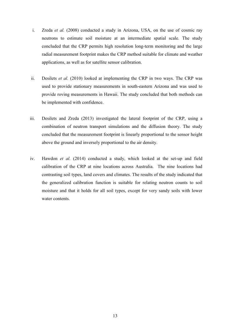
i. Zreda et al. (2008) conducted a study in Arizona, USA, on the use of cosmic ray
neutrons to estimate soil moisture at an intermediate spatial scale. The study
concluded that the CRP permits high resolution long-term monitoring and the large
radial measurement footprint makes the CRP method suitable for climate and weather
applications, as well as for satellite sensor calibration.
ii. Desilets et al. (2010) looked at implementing the CRP in two ways. The CRP was
used to provide stationary measurements in south-eastern Arizona and was used to
provide roving measurements in Hawaii. The study concluded that both methods can
be implemented with confidence.
iii. Desilets and Zreda (2013) investigated the lateral footprint of the CRP, using a
combination of neutron transport simulations and the diffusion theory. The study
concluded that the measurement footprint is linearly proportional to the sensor height
above the ground and inversely proportional to the air density.
iv. Hawdon et al. (2014) conducted a study, which looked at the set-up and field
calibration of the CRP at nine locations across Australia. The nine locations had
contrasting soil types, land covers and climates. The results of the study indicated that
the generalized calibration function is suitable for relating neutron counts to soil
moisture and that it holds for all soil types, except for very sandy soils with lower
water contents.

14
3. REMOTE SENSING OF SOIL MOISTURE
Remote sensing is currently used to measure various parameters of the hydrological cycle,
such as rainfall, evaporation and soil moisture. Remote sensing is seen as a promising
technique for soil moisture estimation, as it aims to address the spatial and temporal
variability of soil moisture (Zhao and Li, 2013). It has the advantages of being able to
measure large scale soil moisture, the data obtained has periodic data updates, its ability to
monitor soil moisture in remote areas, its usability and its cost (Sabins, 2007; Mekonnen,
2009; Lakshmi, 2013). The major limitation to the implementation of remote sensing in
critical hydrological application is its coarse resolution. The following section gives an
overview of the common remote sensing of soil moisture products. This is followed by an
analysis and evaluation of the current downscaling techniques that have been developed to
obtain soil moisture at a finer spatial resolution.
3.1 Overview of Remote Sensing of Soil Moisture
There are several remote sensing techniques that have been developed and applied, which
include gamma radiation, thermal infrared, near infrared and microwave radiation techniques
(Albergel et al., 2012). Each technique measures a different land surface quantity, uses a
different range of the electromagnetic spectrum and has its own unique advantages and
limitations (Mekonnen, 2009). From past research studies, it is evident that the microwave
radiation technique, which consists of both active and passive methods, can be considered as
the most promising technique for the remote sensing of soil moisture. This is due to its
advantages over the other techniques, such as its all-weather capability, large spatial
coverage, temporal resolution, measurement depth and vegetative penetration (Wagner, 2008;
Wang and Qu, 2009; Guillem, 2010).
Microwave radiation remote sensing observes the large contrast in the dielectric properties of
soil particles and water, as well as the dielectric constant increases, as the soil moisture
increases (Mekonnen, 2009; Wang and Qu, 2009). Remote sensing does not measure the soil
moisture content directly, therefore mathematical models that describe the association
between the measured signal and the subsequent soil moisture need to be derived (Wang and
Qu, 2009). Over the past few decades, active and passive microwave remote sensing has
provided the unique ability to obtain estimates of soil moisture on a global scale (Brocca et

15
al., 2013). The L-band range (1 to 10 GHz) is preferably used, as higher frequencies are more
affected by perturbation factors, such as vegetation cover and atmospheric effects (Albergel
et al., 2012). There have been many research studies on microwave remote sensing products
over the past few decades. These products include Soil Moisture and Ocean Salinity (SMOS),
the Advanced Microwave Scanning Radiometer (AMSR2), European Remote Sensing
Satellite (ERS-1/2) and Advanced Scatterometer (ASCAT) (Dorigo et al., 2011).
The remote sensing of soil moisture has advanced and the product user’s trust in the remote
sensing data has increased, as there has been continuous improvements to sensors and the
algorithms used to estimate soil moisture (Brocca et al., 2013). The launch of the SMOS
satellite, which was the first satellite radiometer dedicated to measure soil moisture over land,
emphasized the increased need for the measurement of soil moisture. This is further
highlighted by the anticipated launch of the Soil Moisture Active Passive (SMAP) satellite in
2014 (Jackson et al., 2010; Lakshmi, 2013; Song et al., 2013; Fang and Lakshmi, 2014).
Currently, there are several remote sensing soil moisture products. The two most frequently
utilized products that appear in recent research literature, are the AMSR/AMSR-E
(predecessors of the AMSR2) and SMOS soil moisture products (Brocca et al., 2013). These
two products will be detailed in the subsequent sections.
3.2 AMSR2
The global change observation mission (GCOM) is a project for the global long-term
monitoring of the earth’s environment. The GCOM consists of two satellites, namely, the
GCOM-W and GCOM-C. The GCOM-W1 satellite was launched on the 18th of May 2012
and is equipped with the AMSR2 sensor (Kim et al., 2015). The AMSR2 sensor on the
GCOM-W1 satellite, as seen in Figure 3.1, is the successor to the AMSR sensor on-board the
ADEOS-II satellite, which has been operational from December 2002 to October 2003 and
the AMSR-E sensor, on-board the AQUA satellite, which has been operational from May
2002 to October 2011 (JAXA, 2013a). The basic performance of AMSR2 will be similar to
that of AMSR-E, based on the minimum requirement of data continuity (Imaoka et al., 2010).

16
Figure 3.1 AMSR2 sensor on-board the GCOM-W1 satellite
The AMSR2 sensor is a passive microwave scanning radiometer that makes observations at
multiple polarizations (both horizontal and vertical) and seven frequency bands, ranging from
6.9 GHz to 89 GHz (Kim et al., 2015). It obtains multi-band observations from the C, X and
K bands (Lu et al., 2014). The waves observed are weak and are radiated from the
atmosphere and the earth’s surface. It orbits 700 km above the earth’s surface and has a swath
of 1450 km. Its antenna rotates once every one and a half seconds, which creates a conical
scan pattern, with a scanning interval of 10 km. The scanning method is capable of making
one day (ascending) and one night (descending) observation, covering more than 99% of the
earth’s surface in two days (Lu et al., 2014).
The AMSR2 sensor estimates several of the parameters, which are predominantly linked to
the energy and water cycles, such as precipitation, water vapour, sea-surface temperature, soil
moisture and snow depth. The AMSR2 sensor is more advanced than its predecessors
(AMSR and AMSR-E). It has a larger main reflector with a 2.0 m antenna diameter, which
results in a finer spatial resolution, the addition of a new 7.3 GHz channel to eliminate
electro-magnetic wave interference, an upgraded calibration system and it has intensive
sunlight shielding, to avoid calibration uncertainties (Imaoka et al., 2010; JAXA, 2013a; Kim
et al., 2015)

17
According to JAXA (2013b), the AMSR2 Level Two soil moisture product uses auxiliary
data in the form of global vegetation coverage ratios. It also uses AMSR2 Level One
products, which include 10.6 GHz brightness temperatures (horizontal and vertical
polarisations), 36.5 GHz brightness temperatures (horizontal polarization), latitude and
longitude and observation date.
The AMSR2 Level Two algorithm uses a simple radiative transfer model. The satellite
observed brightness temperature (TB) at the 10.7 GHZ and 36.5 GHz channels, measures the
natural microwave emissions from the land surface (Kim et al., 2015). The algorithm
assumes that the soil temperature is equal to the vegetation canopy temperature and a
constant value of 293 K is used throughout the year (Kim et al., 2015). The AMSR2 soil
moisture algorithm assesses the vegetation effects on microwave emissions paths. This is
important, as vegetation holds a large amount of moisture and thus needs to be evaluated in
order to estimate soil moisture from satellite data. The soil moisture algorithm uses the
polarization index and the index of soil wetness, obtained from TB, to simultaneously
estimate soil moisture and vegetation moisture. With regards to vegetation, the algorithm uses
a look-up table method, where a linear relationship between vegetation water content and
optical depth is applied (Kim et al., 2015). A dielectric mixing model is used in the algorithm
to convert the dielectric constant into soil moisture content (Kim et al., 2015).
3.3 SMOS
The SMOS satellite system, which is illustrated in Figure 3.2, was launched in November
2009 and consists of a space-borne passive microwave L-band (1.4 GHz) interferometric
radiometer (Albergel et al., 2012). The overall aim of SMOS is to provide global surface soil
moisture maps with an accuracy of 4% at a 35 – 50 km spatial resolution (Parrens et al.,
2012). The SMOS satellite has the ability to obtain measurements at multiple angles, which
allows for the retrieval of additional parameters (Kerr et al., 2012). The SMOS system is a Y-
shaped instrument, which consists of 69 antennae. The antennae are equally spaced along
three arms and view the surface of the earth either through full, or two polarized radiances, in
order to provide a full image (Gruhier et al., 2011).

18
Figure 3.2 SMOS satellite
SMOS operates by measuring the phase difference of radiation from various incident angles,
so that the earth’s surface is frequently viewed at different angles and polarizations (Fang and
Lakshmi, 2014). The SMOS soil moisture product has an average spatial resolution of 40 km;
however, this varies from 30-50 km due to, the target area being viewed from multiple angles
(Kerr et al., 2010). SMOS has a sun-synchronous orbit at an altitude of 757 km,
consequently, the entire earth is covered at least twice in three days, with orbit overpasses at
6:00 (ascending) and 18:00 (descending) local standard time (Leroux et al., 2013; Qin et al.,
2013).
L-band radiometry has a high potential for the estimation of surface parameters and has been
recognised as the most promising technique to monitor soil moisture over land surfaces and at
a global scale (Kerr et al., 2012; Parrens et al., 2012). The L-band is the optimum wavelength
range to observe soil moisture, as higher frequencies are more affected by perturbing factors,
including atmospheric effects and vegetative cover (Parrens et al., 2012; Mecklenburg et al.,
2013). The microwave signal at L-band frequency is primarily driven by surface soil moisture
(top 5 cm), effective surface temperature and vegetative opacity, with smaller effects from
the atmosphere and surface characteristics, such as bulk density, soil texture and surface
roughness (Kerr et al., 2012; Leroux et al., 2013). The soil moisture retrieval algorithm needs
to account for all these effects (Kerr et al., 2012).

19
The SMOS Level Two retrieval algorithm is physically-based and complex. It uses the
polarizations and multi-angular information derived by the SMOS satellite and involves the
use of decision trees and direct model inversions (Parrens et al., 2012). The retrieval
algorithm was designed to be easily improved and uses SMOS Level 1C data as input and
uses two types of auxiliary data, namely, static data (soil texture) and dynamic data
(temperature) (Kerr et al., 2012). SMOS provides multi-angular microwave polarimetric
brightness temperature (TB), from which a surface soil moisture product is derived (Parrens et
al., 2012).
The L-band microwave emission of the biosphere model, which simulates the microwave
emission at L-Band range from the soil-vegetation layer is a key component of the retrieval
algorithm (Parrens et al., 2012). This is important, as the major difficulty in the estimation of
soil moisture, using microwave radiometry is due to the presence of dense overlying
vegetation, which attenuates the soil emission and adds its own emission (Parrens et al.,
2012).
The retrieval algorithm is based on an iterative approach. The aim of the algorithm is to
reduce a cost function, the focal constituent of which is the sum of the squared weighted
difference between measured TB and Modelled TB for a collection of incidence angles (Kerr
et al., 2012). In order to reduce this cost function, the most suitable set of parameters needs to
be determined and used to drive the TB model.
Current remote sensing soil moisture products have a spatial pixel grid between 10 to 50 km.
The major issues in the calibration and validation procedure, when using in-situ point
measurements, are the vertical and horizontal scaling issues. The vertical scaling issues occur
when remote sensing soil moisture (top 0.05 m) is calibrated and validated against in-situ soil
moisture measurements (0.00 to 2.00 m) (Jackson et al., 2010). Therefore, the measurements
are at different depths, which is a problem, as soil moisture varies with depth. The horizontal
scaling issues occur when a point measurement is used to validate a remote sensing area-
averaged value. The assumption that the point is representative of a large area can be
conceded to be incorrect, due to the spatial variability of soil moisture (Gruber et al., 2013).
Therefore, there needs to be a shift to area-averaged in-situ methods, to validate and calibrate
remote sensing data.

20
There have been numerous studies on passive microwave remote sensing for soil moisture
estimation. The AMSR-E product is a frequently-used product in past studies. Research
studies that have evaluated surface soil moisture derived from AMSR–E, have shown
promising results (Koike et al., 2004; Draper et al., 2009; Zhang et al., 2011; Qin et al.,
2013). Previous literature has mentioned the launch of the SMOS satellite and how it
emphasizes the value of soil moisture estimation in the science field. SMOS data have been
used in studies which have shown its potential for accurately obtaining soil moisture
measurements (Gruhier et al., 2011; Merlin et al., 2012; Wagner et al., 2012; Mecklenburg et
al., 2013; Qin et al., 2013). Over the past few decades, there have been many studies
involving both the calibration and validation of remote sensing soil moisture products to in-
situ soil moisture measurements (Jackson et al., 2010; Brocca et al., 2011; Fang and
Lakshmi, 2014). The following are some of the remote sensing based soil moisture product
studies:
i. The AMSR2 soil moisture product has been used in a recent study by Lu et al. (2014),
which presented a revised soil moisture retrieval algorithm of AMSR2 and aimed at
improving the soil moisture estimates in dry regions. The study concluded that the
revised algorithm is effective in overcoming the over-estimation of soil moisture in
desert regions.
ii. A recent study by Kim et al. (2015) assessed two versions of the AMSR2 soil
moisture product. The AMSR2 product from the Japan Aerospace Exploration
Agency (JAXA) and Land Parameter Retrieval Model (LPRM) from the VU
University Amsterdam, were used and compared on a global scale against field
measurements. The study used CRP measurements from the COSMOS. It concluded
that the JAXA AMSR2 product has a relatively better performance under dry
conditions; however, the JAXA algorithm generally under-estimates the ground soil
moisture. It also indicated that there is a need to improve both the algorithms and that
a combined product could provide better estimates of soil moisture.
iii. A study by Leroux et al. (2013), compared the SMOS, AMSR-E and ASCAT soil
moisture products over four watersheds in the United States for the year 2010. The
study concluded that the SMOS product correlated the closest to ground

21
measurements, the AMSR-E product gives reasonable results in terms of correlation
and the ASCAT product was unstable.
iv. A study conducted by Albergel et al. (2012) evaluated the ASCAT and SMOS
products against in-situ soil moisture observations from over 200 stations across the
world for the year 2010. A similar study was conducted by Brocca et al. (2011),
which evaluated the ASCAT and AMSR-E satellite-based soil moisture products
around Europe. The main purpose was to evaluate the potential of different ASCAT
and AMSR-E products in obtaining reliable estimates of soil moisture. The study
concluded that the AMSR-E LPRM provided the best results.
3.4 Downscaling Techniques
Microwave remote sensing is extensively used to obtain regional soil moisture estimates,
although its application is greatly restricted by its coarse resolution (Zhao and Li, 2013).
There have been several research studies undertaken to downscale satellite-based soil
moisture estimates for use in hydrological applications (Song et al., 2013). Downscaling is
relevant, as the coarse resolution is at tens to hundreds of kilometres, whereas hydrological
processes occur at spatial scales of centimetres to kilometres (Shin and Mohanty, 2013).
Satellites have the capability to observe and monitor large areas. The subsequent
observational spatial resolution is dependent on the microwave frequency used, the
dimensions of the antenna and the height of the satellite above the earth’s surface (Piles et al.,
2011). There is a trade-off between the temporal and spatial satellite resolution; as the sensor
height decreases, the spatial resolution increases and the temporal resolution decreases
(Merlin et al., 2012).
Over the past decade, a number of downscaling techniques, with varying degrees of
complexity, have been researched and developed (Merlin et al., 2008). An extensive research
paper by Lakshmi (2013) outlines the key publications on current methods used to downscale
passive microwave remote sensing soil moisture products. These studies have reviewed
downscaling procedures, with the use of MODIS sensor-derived parameters, including
surface temperature, vegetation and other ground surface parameters.
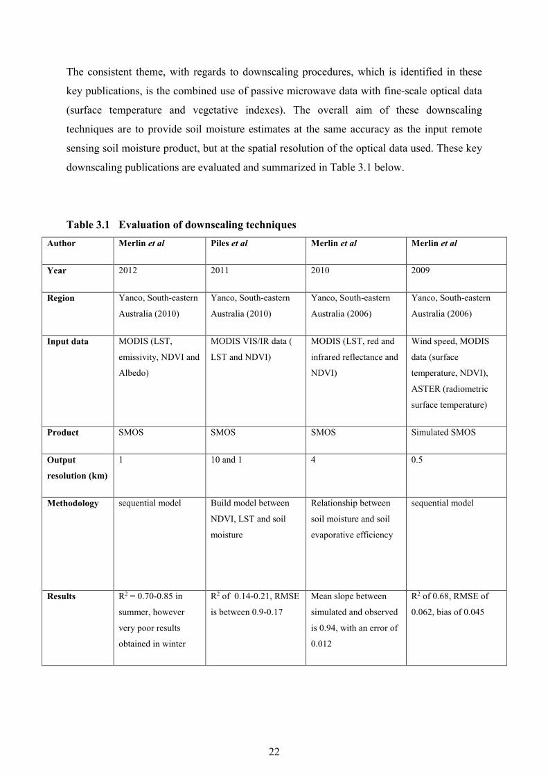
22
The consistent theme, with regards to downscaling procedures, which is identified in these
key publications, is the combined use of passive microwave data with fine-scale optical data
(surface temperature and vegetative indexes). The overall aim of these downscaling
techniques are to provide soil moisture estimates at the same accuracy as the input remote
sensing soil moisture product, but at the spatial resolution of the optical data used. These key
downscaling publications are evaluated and summarized in Table 3.1 below.
Table 3.1 Evaluation of downscaling techniques Author Merlin et al Piles et al Merlin et al Merlin et al
Year 2012 2011 2010 2009
Region Yanco, South-eastern
Australia (2010)
Yanco, South-eastern
Australia (2010)
Yanco, South-eastern
Australia (2006)
Yanco, South-eastern
Australia (2006)
Input data MODIS (LST,
emissivity, NDVI and
Albedo)
MODIS VIS/IR data (
LST and NDVI)
MODIS (LST, red and
infrared reflectance and
NDVI)
Wind speed, MODIS
data (surface
temperature, NDVI),
ASTER (radiometric
surface temperature)
Product SMOS SMOS SMOS Simulated SMOS
Output
resolution (km)
1 10 and 1 4 0.5
Methodology sequential model Build model between
NDVI, LST and soil
moisture
Relationship between
soil moisture and soil
evaporative efficiency
sequential model
Results R2 = 0.70-0.85 in
summer, however
very poor results
obtained in winter
R2 of 0.14-0.21, RMSE
is between 0.9-0.17
Mean slope between
simulated and observed
is 0.94, with an error of
0.012
R2 of 0.68, RMSE of
0.062, bias of 0.045
23
The evaluation of the abovementioned methods highlights significant limitations, which
hinder the successful application of the various downscaling procedures that have been
developed. These include (a) observational days have to be cloud-free, to avoid obscurities in
data retrieval; (b) the presence of vegetation interferes with land surface temperature
retrieval; (c) there is a difference in the input data sensing depth; and (d) the model
assumptions may not be valid in heterogeneous areas (Merlin et al., 2008; 2009; 2010; Piles
et al., 2011).
From the evaluation of these downscaling techniques, several comparisons can be made.
Firstly, all of the downscaling research studies were conducted in the same region; this
simplifies the evaluation process between the different techniques used. It can be noted that
the technique used by Piles et al. (2011) requires the least data input, while the technique
used by Merlin et al. (2009) requires the most input data. All the techniques use SMOS data
or a simulated SMOS data set, as the SMOS satellite is the most recent soil moisture satellite.
The evaluation between the methods is enhanced due to the common aspects of the research
studies.
The differences in the evaluated techniques can be seen in their methodologies, output
resolutions and results. Merlin et al. (2012) had an output resolution of 1 km and showed
good results in summer; however, the technique performed very poorly in winter, when
compared to in-situ soil moisture data. Piles et al. (2011) had an output resolution of 1 and 10
km, but performed poorly, when compared to in-situ soil moisture data. The Merlin et al.
(2010) resulted in the best correlation between observed and simulated soil moisture. Merlin
et al. (2009) showed good correlation and had the finest resolution.
The limitations of the downscaling process can be summarized as follows:
i. The accuracy of the soil moisture product may decrease as the spatial resolution
increases (there is a trade-off between obtaining accurate data and obtaining fine
resolution products);
ii. The process requires input data, which may not be freely or readily available;
iii. The technique may be site-specific;
iv. The complexity of the algorithms used; and
v. Cloud-free images are required, if MODIS products are used.

24
In recent years, the need for fine resolution soil moisture products has resulted in numerous
downscaling research studies being conducted. The main publications in this field have been
studies conducted by Merlin et al. (2009; 2010; 2012) and Piles et al. (2011). In addition to
these, more recent studies have been conducted, which are based on the same principles of
the key techniques. However, there are slight variations, in order to improve and build upon
these key approaches. The new studies include:
i. A study conducted by Zhao and Li (2013) aimed to develop a downscaling method to
improve the spatial resolution of the AMSR-E derived soil moisture product. The
approach was based upon the conventional method of the microwave-optical
synergistic technique, which uses LST, vegetative indexes and albedo. This approach
replaces LST with two temperature temporal variation parameters. The study was
conducted in the Iberian Peninsula for the year 2007. The results showed an
improvement in the approach (R2 increased by 0.08), when the new approach was
compared to the conventional method.
ii. A recent study by Ruiz et al. (2014) was conducted on combining SMOS visible and
near infrared satellite data for high resolution soil moisture over a two-year period in
the REMEDHUS network in Spain. The study used a new downscaling algorithm,
based on a relationship between LST, NDVI and brightness temperature. The study
aimed to obtain a downscaled image with the same accuracy of SMOS, but at the
spatial resolution of MODIS (500 m). The best result obtained was a correlation with
the in-situ measurements of 0.72.
25
4. METHODS OF MODELLING SOIL MOISTURE
Land surface water and surface energy balance models have been used to estimate soil
moisture, as surface soil moisture plays a significant role in controlling the land-atmosphere
water and energy fluxes (Walker and Houser, 2000). Several models have been used to obtain
soil moisture estimates. These include the Variable infiltration capacity (VIC) hydrological
model, the Decision support system for agro-technology transfer crop model (DSSAT), the
climate water budget (CWB), the SEBS, PyTOPKAPI and the Surface Energy Balance
Algorithm for Land (SEBAL) (Meng and Quiring, 2008; Mengistu et al., 2014). The VIC,
DSSAT and CWB are complex models, which require a large amount of input data (Meng
and Quiring, 2008). The SEBAL Model is not freely available to apply due to its intellectual
property rights (Mengistu et al., 2014).
The following section describes the use of the PyTOPKAPI Model soil moisture product and
the SEBS Model to obtain soil moisture estimates. The PyTOPKAPI Model was selected, as
it has been used in South Africa. It is able to provide estimates with a fine spatial and
temporal resolution and the estimates are readily available. The SEBS Model was selected, as
it is an open-source model, it is easy to use and has been validated in several studies
internationally and in South Africa.
4.1 Land Surface Model (PyTOPKAPI)
Soil moisture is a significant parameter in the hydrological cycle and is the prime regulator in
a catchment’s response to precipitation, as it partitions precipitation into infiltration and
surface runoff (Vischel et al., 2008). The topographic kinematic approximation and
integration (TOPKAPI) model was developed by Liu and Todini (2002). The model is fully
distributed and physically-based, as it represents hydrological processes on grid cells, on the
basis of soil physics and fluid mechanics (Vischel et al., 2008). The TOPKAPI Model has
been adapted to perform simulations in land surface modelling mode and its model code has
been adapted, so that it operates as a collection of cells (Sinclair and Pegram, 2010). Each
cell is independent of its neighbours and has a plan area of 1 km x 1 km, with a 0.125o grid
spacing (Sinclair and Pegram, 2010). Each grid cell comprises of three key reservoirs (soil,
overland, channel), as seen in Figure 4.1, which are determined by combing the physically-

26
based mass and continuity equations under the estimate of the kinematic wave model
(Vischel et al., 2008).
Figure 4.1 A schematic of the water transfer in a typical PyTOPKAPI model cell
(Sinclair and Pegram, 2012)
The model is forced by time varying estimates of total evaporation and rainfall for each
model cell (Sinclair and Pegram, 2012). The total evaporation forcing is based on the
modification of the FAO56 reference crop evaporation, whereas the rainfall forcing is applied
in the TRMM 3B42RT product, which is automatically downloaded from the NASA server
and processed locally (Sinclair and Pegram, 2010).
There are six fundamental assumptions on which the TOPKAPI model is based on (Vischel et
al., 2008):
i. Precipitation is spatially and temporally constant over the integration domain;
ii. Unless the soil is already saturated, all precipitation falling on the soil infiltrates;
iii. The slope of the groundwater table corresponds with the slope of the ground;
iv. The saturated hydraulic conductivity in the soil surface layer is constant with depth;
v. Local transmissivity; and
vi. During the transition phase, the variation in water content in time is constant in
space.
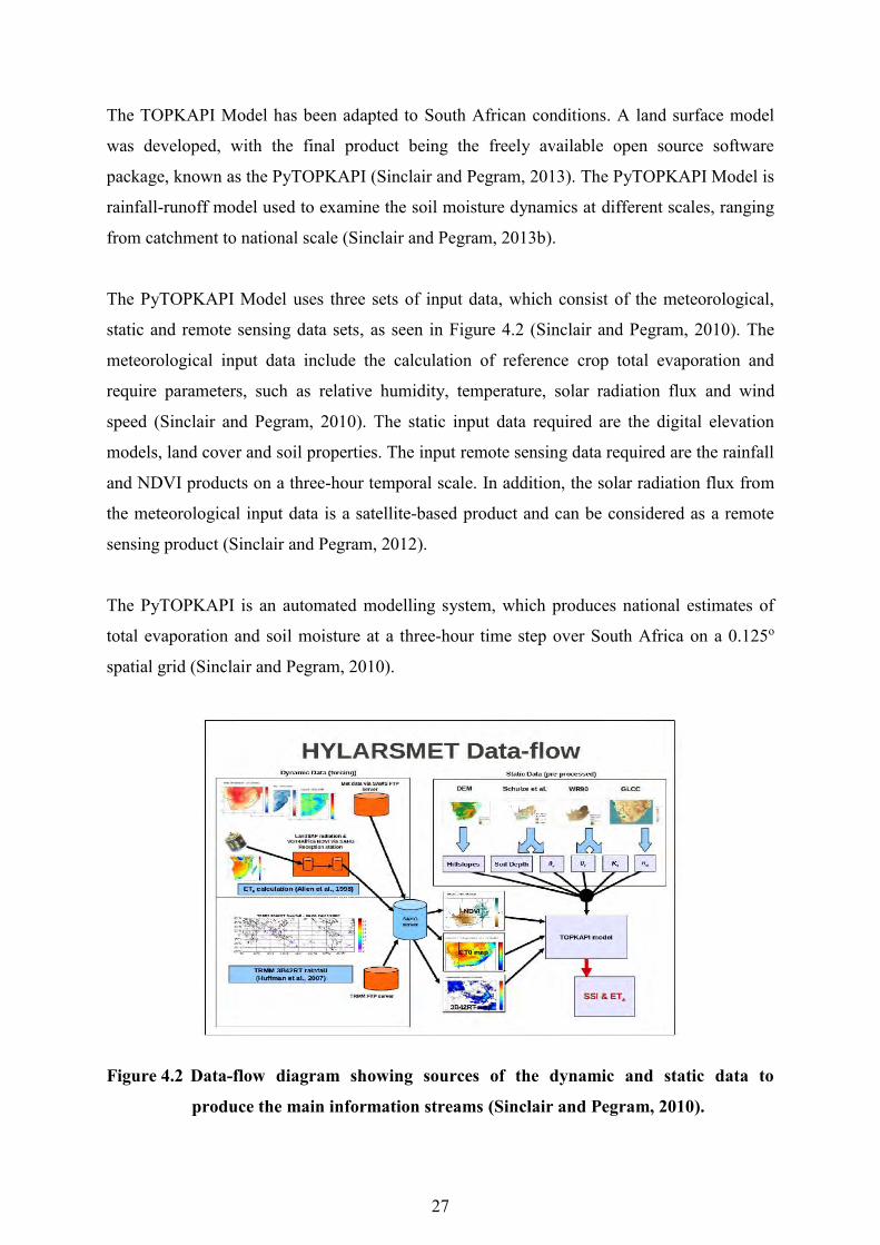
27
The TOPKAPI Model has been adapted to South African conditions. A land surface model
was developed, with the final product being the freely available open source software
package, known as the PyTOPKAPI (Sinclair and Pegram, 2013). The PyTOPKAPI Model is
rainfall-runoff model used to examine the soil moisture dynamics at different scales, ranging
from catchment to national scale (Sinclair and Pegram, 2013b).
The PyTOPKAPI Model uses three sets of input data, which consist of the meteorological,
static and remote sensing data sets, as seen in Figure 4.2 (Sinclair and Pegram, 2010). The
meteorological input data include the calculation of reference crop total evaporation and
require parameters, such as relative humidity, temperature, solar radiation flux and wind
speed (Sinclair and Pegram, 2010). The static input data required are the digital elevation
models, land cover and soil properties. The input remote sensing data required are the rainfall
and NDVI products on a three-hour temporal scale. In addition, the solar radiation flux from
the meteorological input data is a satellite-based product and can be considered as a remote
sensing product (Sinclair and Pegram, 2012).
The PyTOPKAPI is an automated modelling system, which produces national estimates of
total evaporation and soil moisture at a three-hour time step over South Africa on a 0.125o
spatial grid (Sinclair and Pegram, 2010).
Figure 4.2 Data-flow diagram showing sources of the dynamic and static data to
produce the main information streams (Sinclair and Pegram, 2010).

28
The purpose of the computation is to obtain a Saturated Soil Index (SSI), which is defined as
the percentage of the soil voids occupied by water.
𝑆𝑆𝐼 = 100 ∗ (Ɵ−Ɵ𝑟
Ɵ𝑠𝑎𝑡−Ɵ𝑟) (4.1)
Where Ɵ is the volumetric soil moisture, Ɵr is the residual soil moisture and Ɵsat is the
saturated soil moisture.
In the original design, Liu and Todini (2002) created the model in such a manner, that
whether the soil store was saturated or not, all rainfall during the computational interval was
added to the soil store. At the end of the interval, an inventory was made and if the store was
full, the excess was assigned to overland and channel stores. Then, based on the content of
the soil store, the drainage was sent to the downslope store (Sinclair and Pegram, 2013a).
This resulted in two effects: the soil store was always depleted at the end of the computation
interval and surface runoff only occurred once the soil store was full, independent of rainfall
intensity (Sinclair and Pegram 2013).
In the adaption of the TOPKAPI Model to South African conditions, the first effect was
cancelled by modifying the continuity equation, so that there was ponding in the overland
store, which resulted in the soil store remaining full after computation (Sinclair and Pegram,
2013a). The second effect was dealt with the introduction of the Green-Ampt infiltration
model, which gave the PyTOPKAPI Model the ability to generate rapid overland flows in
response to intense rainfall events (Sinclair and Pegram 2013).
The benefits of using this model are that the soil moisture estimates obtained have a temporal
resolution of three hours and a spatial resolution grid ≈ 12.5 km. This finer temporal and
spatial resolution better accounts for the heterogeneity of soil moisture, compared to the
current global remote sensing of soil moisture products.
There have been research studies that reviewed the estimation of soil moisture through land
surface modelling.

29
i. Sinclair and Pegram (2010) conducted a study, which aimed to compare soil moisture
estimates from two independent sources over South Africa. The first soil moisture
estimate was provided by automated real-time estimates from the TOPKAPI
hydrological model. The second set of soil moisture estimates was from the ASCAT
remote sensing product.
ii. A similar study was conducted by Vischel et al. (2008) in the Liebenbergslvei
Catchment in South Africa, which compared soil moisture estimates derived from the
TOPKAPI Model with European remote sensing satellite-based soil moisture
estimates. Both studies concluded that the modeled soil moisture measurements
correlated well, when compared to remote sensing soil moisture measurements.
iii. More recent studies, conducted by Sinclair and Pegram (2013), evaluated the
sensitivity of the PyTOPKAPI Model to systematic bias in the variables of soil
properties, evapotranspiration and rainfall. This was achieved by analysing 7200 sites
within South Africa for a two-and-a-half year simulation period. The study concluded
that the model is robust to errors in forcing parameters.
iv. A study conducted by Mengistu et al. (2014) involved the validation of variables of
the PyTOPKAPI Model. The aims of the study were to provide data for the soil
moisture mapping of South Africa, using the PyTOPKAPI Model. The purpose was to
provide accurate field and satellite estimates of total evaporation and soil moisture for
the calibration of the model and to evaluate the spatial variability of soil moisture at a
catchment scale.
4.2 Surface Energy Balance System (SEBS)
Over the past few decades, several methods of estimating evaporation have been developed
and implemented (Ma et al., 2012). The SEBS Model was developed by Su (2002) for the
estimation of atmospheric turbulent fluxes and surface evaporative fraction, using remote
sensing data (Su et al., 2003). The SEBS Model is physically-based, has the advantage of
being less site-specific, open-source, it has been applied extensively (especially as an
academic tool for research purposes) and does not require subjective intervention by the
model user (Gokman et al., 2012).

30
The model requires three sets of informational input data. The first set comprises of albedo,
temperature, leaf area index and vegetation coverage (Su, 2002). In cases where this
information is unavailable, the NDVI and the vegetation height are used instead. These
informational inputs can be obtained from remote sensing data, in conjunction with additional
land surface information. The second set of information comprises the reference boundary
layer height (Su, 2002). The third set of input data required is the downward solar and long-
wave radiation, which are obtained either from direct measurement, parameterization or
model output (Su, 2002).
The SEBS Model consists of numerous individual components, to estimate the net radiation
and soil heat flux and to partition the available energy into latent and sensible heat fluxes.
The Surface Energy Balance is expressed as follows (Equation 4.2) (Wang and Li, 2011):
Rn = G𝑜 + H+ λE (4.2)
Where Rn = net radiation, Go = soil heat flux, H = sensible heat flux and λE = latent heat flux.
The considerations of the surface energy balance, at limiting cases, are used to determine the
relative evaporation (Wang and Li, 2011). When the dry limit is considered, the latent heat is
zero and the sensible heat flux is at its maximum (Wang and Li, 2011):
λEdry = Rn − Go − Hdry ≡ 0
Hdry = Rn − Go (4.3)
When the wet limit is considered, evaporation occurs at a maximum rate, whilst the sensible
heat flux takes the minimum value (Wang and Li, 2011):
λEwet = Rn − Go − Hwet (4.4)
The relative evaporation can be expressed as (Su et al., 2003):

31
Λr = λE
λEwet= 1 −
λEwet − λE
λEwet (4.5)
By substituting Equations 4.2 – 4.4 in Equation 4.4 and rearranging (Su et al., 2003):
Λr = 1 − H− Hwet
Hdry− Hwet (4.6)
Applying the mass conservation principle and integrating with respect to depth and time
increments (Su et al., 2003):
∫ θ(z, t2)dz − ∫ θ(z, t1)dz = Q(z1) − Q(z2)z2
z1
z2
z1 (4.7)
where θ is the volumetric soil moisture content, t is the time and z is the vertical distance.
Applying Equation 4.7 with boundary conditions Q (z1) = Po + Io –E at the soil surface and Q
(z2) = Ic at the bottom of the rooting zone. The change in soil water content can be expressed
as (Su et al., 2003):
Θ(t2) − Θ(t1) = Po + Io + Ic − E (4.8)
where Θ is the volumetric soil water content in the rooting zone, Po is the precipitation, Io is
the irrigation, Ic capillary flux and E is evaporation. The water balance is then considered at
limiting cases. The wet limit is saturation, so that Θ (t1) = Θwet. At the dry limit Θ (t2) = Θdry,
the evaporation is zero. From Equation 4.8 (Su et al., 2003):
Θwet − Θdry = Icwet − Ewet (4.9)
For any time between the two boundary conditions:
Θ − Θdry = Icwet − E (4.10)
Manipulating Equation 4.9 and Equation 4.10 (Su et al., 2003):
Θ − Θdry
Θwet− Θdry=
E−Ic
Ewet−Icwet (4.11)

32
It is assumed that the capillary flux is linked to the soil texture and is less than that of the
uptake of root water (Ic = Iwet). By defining Rθ = Θ/ Θwet as the relative soil water content and
using Equation 4.11 (Su et al., 2003):
Rθ = Θ
Θwet=
λE
λEwet (4.12)
This inverse relationship is often used in hydrological modelling and can be expressed as:
λE
λEwet= f (
SMactual
SMfield capacity) = Ʌ (4.13)
The relative evaporation is therefore calculated as the relative soil moisture contained in the
rooting zone. The term f is used as a linear relationship. The SM field capacity can be inferred
from the soil texture.
An alternative method, which uses an empirical relationship between the evaporative fraction
and soil moisture, was developed by Bastiaanssen et al. (1997). The equation is based on two
large-scale climate-hydrology studies, which investigated the interactions between soil
moisture, evaporation and biomass (Scott et al., 2003; Bezerra et al., 2013). The empirical
equation was modified by Scott et al. (2003), by standardizing soil moisture with saturated
soil moisture, to create relative soil moisture content (Scott et al., 2003):
θ
θsat= exp[(ᴧ−1)/0.421] (4.14)
These methods of soil moisture estimation result in a finer spatial resolution than that of
current remote sensing soil moisture products, as the remotely sensed data is observed at a
finer spatial scale. In addition, the soil moisture being estimated is at a greater depth than that
estimated by microwave remote sensing (Bezerra et al., 2013). The limitation of this method
is that the observations and measurements are restricted to cloudless days, as retrieval is
affected by atmospheric conditions. Therefore, only days which are cloud-free can be used, in
order to reduce measurement errors.

33
The SEBS Model has been applied globally in several studies (Wang and Li, 2011; Gokman
et al., 2012; Ma et al., 2012).
i. A study conducted by Su et al. (2003) derived a measure for the quantification of
drought severity. The study used the SEBS Model, meteorological data and NOAA
satellite images to derive relative evaporation in North China. A drought severity
index (DSI) was subsequently derived from the relative evaporation. The DSI gives
an indication of the soil moisture status, so that a high relative evaporation is
associated with a high soil moisture status. The study concluded that the DSI and
actual soil moisture measurements show a good comparison.
ii. Studies conducted by Scott et al. (2003) and Bezerra et al. (2013) evaluated the
relationship to calculate soil moisture from remote sensing data. The study conducted
by Bezerra et al. (2013) was carried out in the Apodi Plateau in Brazil. The study
concluded that there was a close correlation between measured and estimated soil
moisture value (R2=0.84).
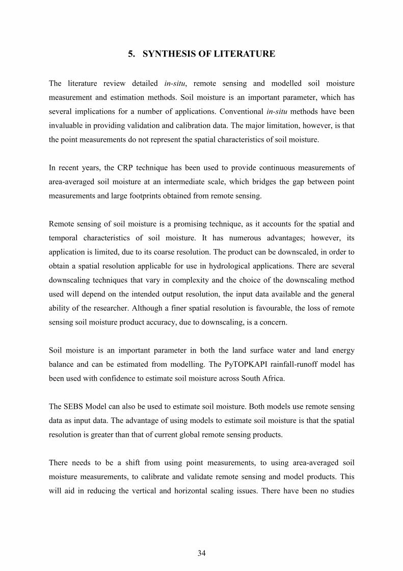
34
5. SYNTHESIS OF LITERATURE
The literature review detailed in-situ, remote sensing and modelled soil moisture
measurement and estimation methods. Soil moisture is an important parameter, which has
several implications for a number of applications. Conventional in-situ methods have been
invaluable in providing validation and calibration data. The major limitation, however, is that
the point measurements do not represent the spatial characteristics of soil moisture.
In recent years, the CRP technique has been used to provide continuous measurements of
area-averaged soil moisture at an intermediate scale, which bridges the gap between point
measurements and large footprints obtained from remote sensing.
Remote sensing of soil moisture is a promising technique, as it accounts for the spatial and
temporal characteristics of soil moisture. It has numerous advantages; however, its
application is limited, due to its coarse resolution. The product can be downscaled, in order to
obtain a spatial resolution applicable for use in hydrological applications. There are several
downscaling techniques that vary in complexity and the choice of the downscaling method
used will depend on the intended output resolution, the input data available and the general
ability of the researcher. Although a finer spatial resolution is favourable, the loss of remote
sensing soil moisture product accuracy, due to downscaling, is a concern.
Soil moisture is an important parameter in both the land surface water and land energy
balance and can be estimated from modelling. The PyTOPKAPI rainfall-runoff model has
been used with confidence to estimate soil moisture across South Africa.
The SEBS Model can also be used to estimate soil moisture. Both models use remote sensing
data as input data. The advantage of using models to estimate soil moisture is that the spatial
resolution is greater than that of current global remote sensing products.
There needs to be a shift from using point measurements, to using area-averaged soil
moisture measurements, to calibrate and validate remote sensing and model products. This
will aid in reducing the vertical and horizontal scaling issues. There have been no studies

35
conducted in South Africa on the comparison of soil moisture estimate methods, using the
CRP as validation data for satellite-based soil moisture estimates.
From the literature reviewed, the gaps in past research studies have become apparent. A
major gap has been the use of point measurements for the calibration and validation of
remote sensing and modelled soil moisture estimates. This has resulted in horizontal and
vertical scaling issues, therefore there is a need for a shift towards the use of area-average
calibration and validation data, in order to bridge the gap between scales.
Downscaling procedures have not been used in South African case studies; however, they are
essential in obtaining remote sensing soil moisture estimates at a fine spatial resolution,
which can be used in hydrological applications. Where downscaling has been used, the
downscaled estimates were compared to point measurements.
The PyTOPKAPI Model has been implemented in South Africa with confidence; however,
its estimates have not been evaluated against area-averaged soil moisture measurements.
There have been no South African case studies on the CRP, therefore a comprehensive
evaluation of the current methods of soil moisture against the area-averaged soil moisture
measurements obtained from the CRP, need to be conducted in South Africa.

36
6. METHODOLOGY
Several studies referred in the literature review component (chapters two, three and four)
have suggested that the current methods of soil moisture estimation do not adequately
provide measurements for critical hydrological applications, as each method has its
limitations. Although the current methods can provide accurate estimates of soil moisture, the
representativeness of these methods may vary at different spatial scales. These methods need
to be evaluated and improved, in order to obtain soil moisture data that can be used in critical
hydrological applications. Further research is warranted. The following research questions
have been formulated to address both the general and specific objectives of the study:
How suitable is the CRP technique in providing spatial estimates of soil moisture?
How accurate are the Level Three AMSR2 and SMOS soil moisture estimates?
How suitable are the PyTOPKAPI Model product and the back-calculation using the
SEBS model in providing estimates of soil moisture?
What are the effects of seasonality on the different methods of soil moisture
estimation?
The general objectives of this study were to calibrate and validate the CRP and subsequently
use the calibrated CRP soil moisture estimates to validate satellite-based soil moisture
estimates. This involved setting up the CRP in Cathedral Peak Catchment VI. The CRP
continuously monitored soil moisture at an hourly time-step. During this time, four
calibrations were undertaken to determine the representative gravimetric water content of the
study area on that calibration day. An in-situ soil moisture network was also set up that
consisted of TDR and Echo probes. The aim of the in-situ soil moisture measurements was to
provide data that could be used to create a representative soil moisture dataset of the study
area, which could then be used to validate the CRP.
Calibrated CRP estimates were then used to validate satellite-based soil moisture estimates.
These consisted of remote sensing products, back-calculated soil moisture using outputs from
the SEBS model and modelled soil moisture product from the PyTOPKAPI model. Although
the downscaling of remote sensing data was reviewed and evaluated in the literature, the
procedure of downscaling remote sensing products did not fall within the scope of this study
and therefore, was not applied.

37
6.1 Study Site
The study site for this research was Cathedral Peak Research Catchment VI. Cathedral Peak
was established in 1935, as the chief centre for forest hydrological research in the summer
rainfall region (Scott et al., 2000). Its primary purpose was to examine the influences of
various management practices on the vegetation and yield of the local mountainous
catchments (Everson et al., 1998). Cathedral Peak lies within KwaZulu-Natal, in the Tugela
Catchment, as shown in Figure 6.1. It comprises of fifteen gauged catchments that are
situated on the little Berg, located below the Drakensberg escarpment, which creates a natural
border between the north-eastern side of Lesotho and South Africa (Gush et al., 2002).
Figure 6.1 Location of Cathedral Peak Catchment VI, within the Tugela catchment,
within KwaZulu-Natal
The Drakensberg mountain range is the highest mountain range in South Africa and gives rise
to many of the rivers, which are of great economic importance to the country (Everson et al.,
1998). The fifteen research catchments (numbered I to XV) received different land
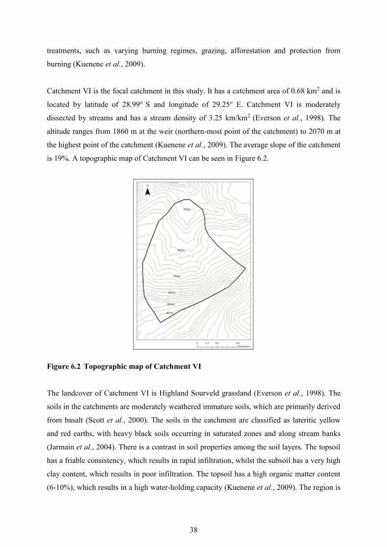
38
treatments, such as varying burning regimes, grazing, afforestation and protection from
burning (Kuenene et al., 2009).
Catchment VI is the focal catchment in this study. It has a catchment area of 0.68 km2 and is
located by latitude of 28.99o S and longitude of 29.25o E. Catchment VI is moderately
dissected by streams and has a stream density of 3.25 km/km2 (Everson et al., 1998). The
altitude ranges from 1860 m at the weir (northern-most point of the catchment) to 2070 m at
the highest point of the catchment (Kuenene et al., 2009). The average slope of the catchment
is 19%. A topographic map of Catchment VI can be seen in Figure 6.2.
Figure 6.2 Topographic map of Catchment VI
The landcover of Catchment VI is Highland Sourveld grassland (Everson et al., 1998). The
soils in the catchments are moderately weathered immature soils, which are primarily derived
from basalt (Scott et al., 2000). The soils in the catchment are classified as lateritic yellow
and red earths, with heavy black soils occurring in saturated zones and along stream banks
(Jarmain et al., 2004). There is a contrast in soil properties among the soil layers. The topsoil
has a friable consistency, which results in rapid infiltration, whilst the subsoil has a very high
clay content, which results in poor infiltration. The topsoil has a high organic matter content
(6-10%), which results in a high water-holding capacity (Kuenene et al., 2009). The region is
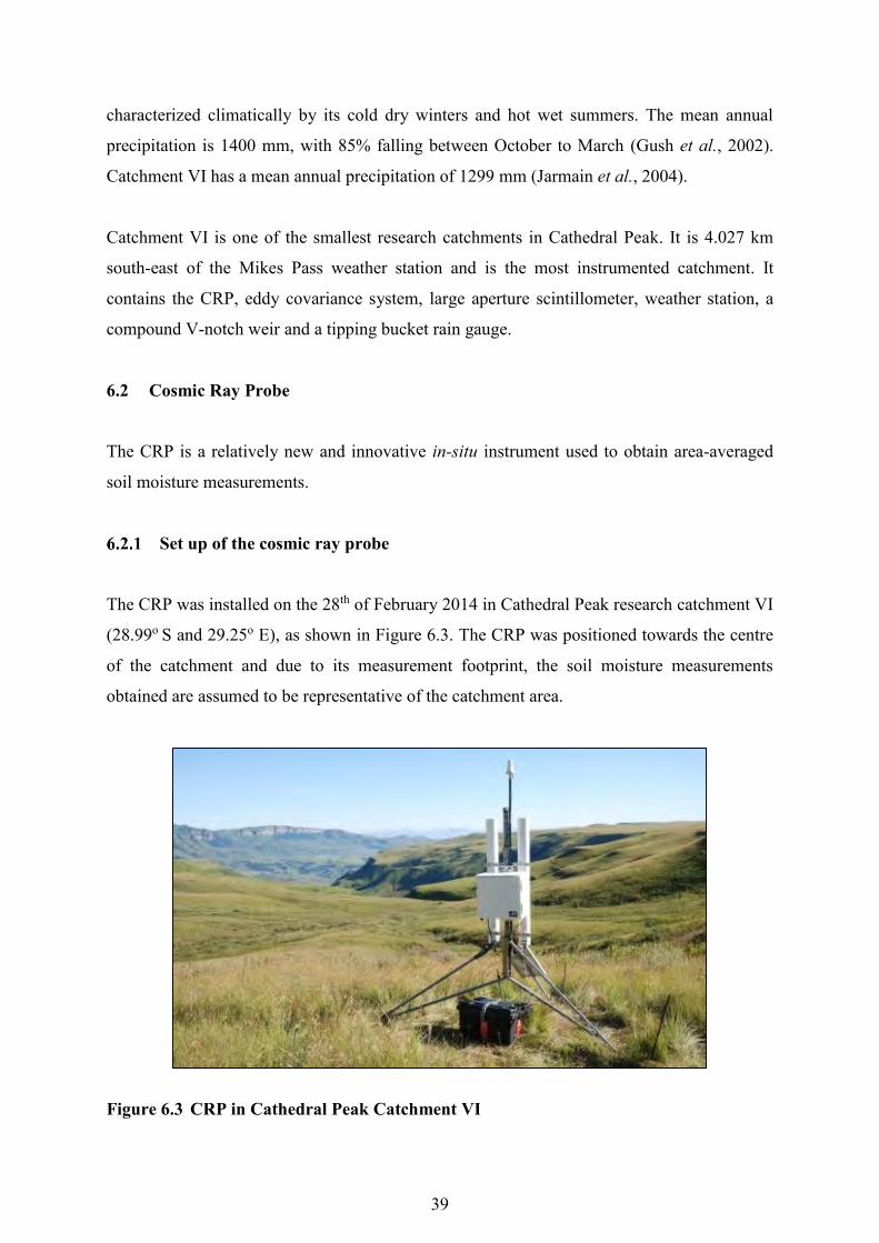
39
characterized climatically by its cold dry winters and hot wet summers. The mean annual
precipitation is 1400 mm, with 85% falling between October to March (Gush et al., 2002).
Catchment VI has a mean annual precipitation of 1299 mm (Jarmain et al., 2004).
Catchment VI is one of the smallest research catchments in Cathedral Peak. It is 4.027 km
south-east of the Mikes Pass weather station and is the most instrumented catchment. It
contains the CRP, eddy covariance system, large aperture scintillometer, weather station, a
compound V-notch weir and a tipping bucket rain gauge.
6.2 Cosmic Ray Probe
The CRP is a relatively new and innovative in-situ instrument used to obtain area-averaged
soil moisture measurements.
Set up of the cosmic ray probe
The CRP was installed on the 28th of February 2014 in Cathedral Peak research catchment VI
(28.99o S and 29.25o E), as shown in Figure 6.3. The CRP was positioned towards the centre
of the catchment and due to its measurement footprint, the soil moisture measurements
obtained are assumed to be representative of the catchment area.
Figure 6.3 CRP in Cathedral Peak Catchment VI
40
The CRP method requires calibration to obtain accurate soil moisture estimates. The
calibration process involves obtaining an estimate of the area-averaged soil moisture content
over the CRP measurement footprint by gravimetric sampling. Soil samples were taken at
three radial rings, extending outwards from the CRP. The radial rings were situated at a
distance of 25 m (A), 100 m (B) and 200 m (C) from the CRP, as shown in Figure 6.4. At
each of the three rings, eight points were taken at an equal distance along the circumference
of the ring. Therefore, points were taken at 0, 45, 90, 135, 180, 225, 270 and 315 degrees
from the CRP.
The location of these 24 points (3 rings x 8 points) were mapped, using GIS software and
their coordinates were recorded (Table 6.1). These points are located within Catchment VI, as
illustrated in Figure 6.5.
A1
A2
A3
A4
A5
A6
A7
A8
B1
B2
B3
B4
B5
B6
B7
B8
C1
C2
C3
C4
C5
C6
C7
C8
CRP
25m
100m
200m
CRP
Figure 6.4 Diagram of sampling points

41
Table 6.1 Geographical coordinates of sample points
Sample Latitude Longitude Sample Latitude Longitude Sample Latitude Longitude A1 -28.9929 29.2519 B1 -28.9922 29.2519 C1 -28.9913 29.2519 A2 -28.9929 29.2520 B2 -28.9924 29.2526 C2 -28.9918 29.2533 A3 -28.9931 29.2521 B3 -28.9931 29.2529 C3 -28.9931 29.2539 A4 -28.9932 29.2520 B4 -28.9937 29.2526 C4 -28.9944 29.2533 A5 -28.9933 29.2519 B5 -28.9940 29.2519 C5 -28.9949 29.2519 A6 -28.9932 29.2517 B6 -28.9937 29.2511 C6 -28.9944 29.2504 A7 -28.9931 29.2516 B7 -28.9931 29.2508 C7 -28.9931 29.2498 A8 -28.9929 29.2517 B8 -28.9924 29.2511 C8 -28.9918 29.2504
Figure 6.5 Position of calibration sample points within Cathedral Peak Catchment VI
C1
B1
A1
A5
B5
C5
A3 B3 C3 A7 B7 C7
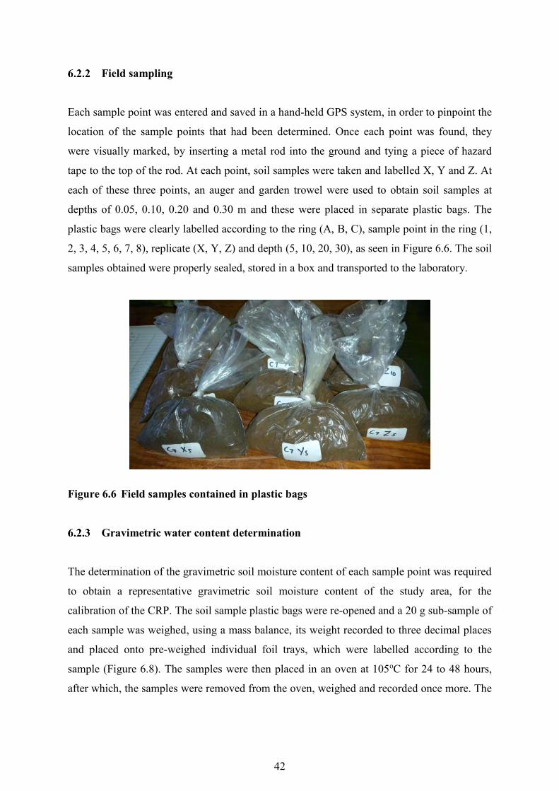
42
Field sampling
Each sample point was entered and saved in a hand-held GPS system, in order to pinpoint the
location of the sample points that had been determined. Once each point was found, they
were visually marked, by inserting a metal rod into the ground and tying a piece of hazard
tape to the top of the rod. At each point, soil samples were taken and labelled X, Y and Z. At
each of these three points, an auger and garden trowel were used to obtain soil samples at
depths of 0.05, 0.10, 0.20 and 0.30 m and these were placed in separate plastic bags. The
plastic bags were clearly labelled according to the ring (A, B, C), sample point in the ring (1,
2, 3, 4, 5, 6, 7, 8), replicate (X, Y, Z) and depth (5, 10, 20, 30), as seen in Figure 6.6. The soil
samples obtained were properly sealed, stored in a box and transported to the laboratory.
Figure 6.6 Field samples contained in plastic bags
Gravimetric water content determination
The determination of the gravimetric soil moisture content of each sample point was required
to obtain a representative gravimetric soil moisture content of the study area, for the
calibration of the CRP. The soil sample plastic bags were re-opened and a 20 g sub-sample of
each sample was weighed, using a mass balance, its weight recorded to three decimal places
and placed onto pre-weighed individual foil trays, which were labelled according to the
sample (Figure 6.8). The samples were then placed in an oven at 105oC for 24 to 48 hours,
after which, the samples were removed from the oven, weighed and recorded once more. The

43
gravimetric water content was then calculated on a wet basis, using the gravimetric water
content:
Gravimetric water content = Wet mass−Dry mass
Dry mass × 100 (6.1)
Figure 6.7 Weighing the soil samples and placing them in the oven
Four calibrations were carried out over a period of eight months. The calibration dates were
the 9th of July 2014, the 28th of August 2014, the 2nd of December 2014, and on the 22nd of
January 2015.
Creating a soil moisture network
It was essential to create a soil moisture network comprising of in-situ soil moisture
measurement instruments at several locations within the CRP measurement area. This was
required in order to obtain data that could be used to validate the CRP measurements. There
were three sets of measurement instruments installed between the 9th and 10th of July 2015. A
soil pit was dug and TDR probes were inserted horizontally at depths of 0.05, 0.10, 0.15, 0.20
and 0.30 m, as illustrated in Figure 6.7 (a). Five wireless TDR sensors (0.12 m) were inserted
vertically into the soil surface at sample points A5, B5, C5, A7 and B7, as illustrated in
Figure 6.7 (b). Shallow soil pits were dug at A1, B1, C1, A3, B3, C3, B7 and C7, and Echo
probes were inserted horizontally at a depth of 0.10 m (Figure 6.7 (c)). The echo probes were
buried and their data loggers were attached to the metal rod at the subsequent sample points
(Figure 6.7 (d)).

44
(a) (b)
(c) (d)
Figure 6.8 (a) Setting up the TDR pit, (b) Wireless TDR, (c) Echo probe and (d) Data
Hobo Onset logger for the Echo probe
The wireless TDR sensors, which were placed on the 10th of July 2014 at points A7, A5, B5,
B7 and C5, were removed on the 28th of August 2014 to check a problem with the data
logging program.
Catchment burning
Catchment VI is subjected to prescribed burning for fire protection and management
purposes, as it reduces the amount of groundcover vegetation during the drier (cooler) months
and decreases the risk of wildfires. These wildfires could cause greater damage later on in the
season. Without fire, grasslands could transform into shrub-lands or forests. Prescribed
burning is different to wildfires and has less of an environmental impact. Prescribed burning
is undertaken by a team of skilled and equipped laborers, who use firebreaks to control the
burning stretch. There are three main types of burning strategies used:
45
i. Back-burning is the technique of setting small fires along a fire-break and burning
back to the main fire front. This burning type is usually against the ground-level
winds and often downslope, which results in a lower intensity fire that moves at a
slower speed, which makes the fire easier to control.
ii. Head-burning is the technique of burning with the ground-level wind direction and is
usually upslope. This burning type has a high intensity and moves at a faster rate,
which makes it harder to control.
iii. Flanking is the technique of setting a fire, which moves parallel to and into the wind.
This burning type is used to supplement the other two burning techniques.
The hydrological consequences of fire include the removal of vegetation cover and the direct
effect of the fire heating the soil (Scott, 1994). The removal of the vegetation cover could
have an impact on the soil moisture status, as the soil surface has greater exposure to
atmospheric conditions. This could lead to increased soil evaporation, which could result in
drier topsoils (Stoof et al., 2012). Conversely, there could be an increase in soil moisture in
the subsoils, due to a reduction in transpiration (Stoof et al., 2012). The removal of
vegetation may also result in increased erosion and sedimentation, due to an increased
exposure of the soil surface to raindrop impact (Scott, 1994). There is a possibility of post-
fire pore-clogging by infiltrated ash, which leads to reduced infiltration rates and causes an
increase in overland-flow (Stoof et al., 2012). There could also be the development of soil
water repellency during and after the fire.
Although these hydrological consequences have been reported, the effects of fire on
hydrological responses at a catchment scale are minor, as these fires are generally prescribed
burns and the issue of scale plays a significant role in the overall change detection of the
hydrological system (Scott, 1994).
On the 5th of September, a scheduled burning from an adjacent Catchment (VII) spread and
caused the unscheduled burning of Catchment VI. As a result of the fire, the Echo probe soil
moisture sensors were destroyed. However, the data from the hobo loggers were retrieved
(Figure 6.9). The larger equipment in Catchment VI were not harmed due to the fire breaks,
as seen in Figure 6.10. Due to the loss of the echo probe sensors, the wireless TDR sensors
had to be placed, to best represent the catchment. This was done by identifying the wet,

46
intermediate and dry areas of the catchment, by using the soil moisture map obtained from
the first calibration.
Figure 6.9 Data retrieved from burned echo probe data loggers
Figure 6.10 Protection of equipment by fire breaks in Catchment VI
Bulk density determination
The gravimetric determination technique was used for the calibration of the CRP. The
gravimetric soil moisture content is expressed, by weight, as the ratio of the mass of water
present to the dry weight of the soil sample (g/g). The CRP, however, measures the
volumetric soil moisture content, which is expressed, as the ratio of volume of water to the
total volume of the soil sample (cm3/cm3). This is further expressed as volumetric water
content in percentage.

47
The calibration of the CRP requires a representative bulk density value, to convert the
gravimetric soil moisture content to volumetric water content. In order to convert gravimetric
soil moisture into volumetric soil moisture, the gravimetric water content is multiplied by the
bulk density. The bulk density determination was carried out on the 2nd of December 2014.
Undisturbed soil cores were taken at three locations in the catchment, corresponding with
three sample points (C1, CRP and C5) and at three depths (0.00 – 0.05 m, 0.05 – 0.10 m and
0.10 – 0.15 m). These sites were selected to best represent the catchment.
At each of the three sites, steel cylindrical cores were inserted vertically into the soil. Starting
with the 0.00 – 0.05 m measurement, the steel core was placed on the surface of the soil. A
wooden board was placed on the top of the core and the core was hammered down into the
soil. The wooden board was used to distribute the force of the hammer on the steel core, so
that the core moves down equally. Once the steel core had reached its intended depth, the soil
around the core was loosened and removed carefully. The steel core was then removed,
clearly labeled and its ends tightly sealed. The same procedure was then carried out at 0.05 –
0.10 m and 0.10 – 0.15 m depths.
The soil cores were then transported to the laboratory, where they were opened carefully. A
knife was used to trim the excess soil of the ends of each side of the core, so that the volume
of the soil equaled the volume of the core. The soil cores (steel core and soil) were oven-dried
at 105oC for 48 hours. The mass of the soil cores were weighed and recorded after oven
drying (refer to Figure 7.14). The mass of the cylindrical steel cores were recorded and
subtracted from the soil core mass, to obtain the mass of dry soil. The volumes of the soil
cores were determined by the dimensions of the cylindrical steel cores. The volume of the
steel core is the volume of the soil.
The bulk densities were calculated, using Equation 6.2:
Bulk Density (g/cm3) = 𝐷𝑟𝑦 𝑀𝑎𝑠𝑠 𝑜𝑓 𝑠𝑜𝑖𝑙 (𝑔)
𝑇𝑜𝑡𝑎𝑙 𝑉𝑜𝑙𝑢𝑚𝑒 (𝑐𝑚3) (6.2)
The calculated bulk densities of each sample point and depth along with the variables used to
calculate them are illustrated in Table 6.2.
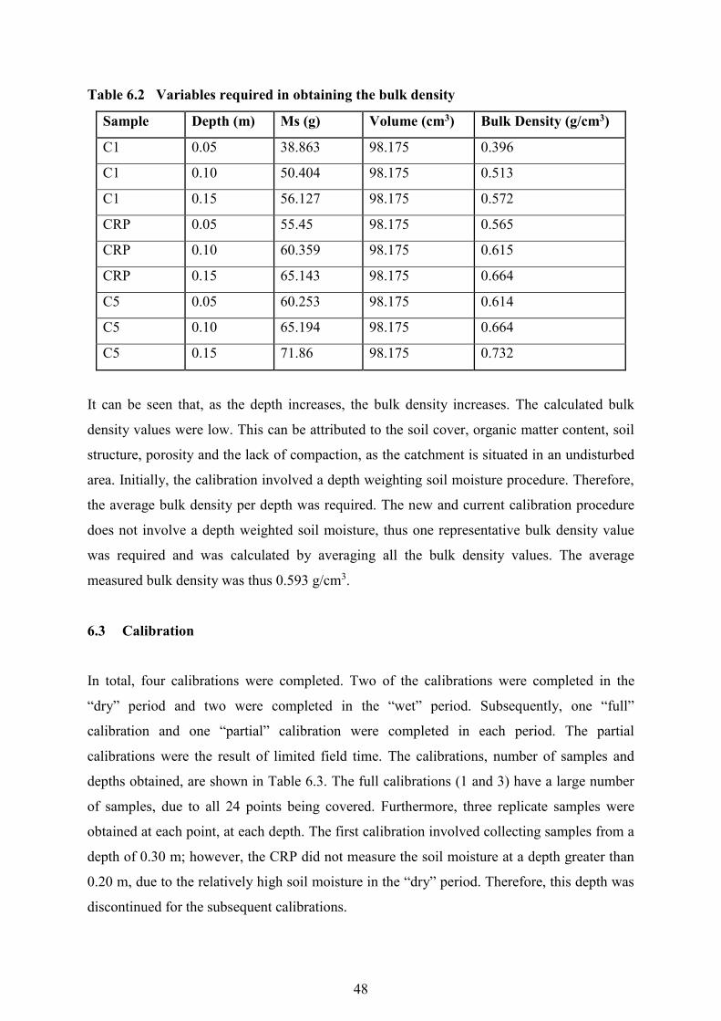
48
Table 6.2 Variables required in obtaining the bulk density
Sample Depth (m) Ms (g) Volume (cm3) Bulk Density (g/cm3)
C1 0.05 38.863 98.175 0.396
C1 0.10 50.404 98.175 0.513
C1 0.15 56.127 98.175 0.572
CRP 0.05 55.45 98.175 0.565
CRP 0.10 60.359 98.175 0.615
CRP 0.15 65.143 98.175 0.664
C5 0.05 60.253 98.175 0.614
C5 0.10 65.194 98.175 0.664
C5 0.15 71.86 98.175 0.732
It can be seen that, as the depth increases, the bulk density increases. The calculated bulk
density values were low. This can be attributed to the soil cover, organic matter content, soil
structure, porosity and the lack of compaction, as the catchment is situated in an undisturbed
area. Initially, the calibration involved a depth weighting soil moisture procedure. Therefore,
the average bulk density per depth was required. The new and current calibration procedure
does not involve a depth weighted soil moisture, thus one representative bulk density value
was required and was calculated by averaging all the bulk density values. The average
measured bulk density was thus 0.593 g/cm3.
6.3 Calibration
In total, four calibrations were completed. Two of the calibrations were completed in the
“dry” period and two were completed in the “wet” period. Subsequently, one “full”
calibration and one “partial” calibration were completed in each period. The partial
calibrations were the result of limited field time. The calibrations, number of samples and
depths obtained, are shown in Table 6.3. The full calibrations (1 and 3) have a large number
of samples, due to all 24 points being covered. Furthermore, three replicate samples were
obtained at each point, at each depth. The first calibration involved collecting samples from a
depth of 0.30 m; however, the CRP did not measure the soil moisture at a depth greater than
0.20 m, due to the relatively high soil moisture in the “dry” period. Therefore, this depth was
discontinued for the subsequent calibrations.

49
Table 6.3 Information regarding the calibration sampling
Depth Measured (m)
Calibration Date Period No. of samples 0.05 0.10 0.20 0.30
1 (Full) July 9, 2014 Dry 288 x x x x
2 (Partial) August 28, 2014 Dry 36 x x x -
3 (Full) December 2, 2014 Wet 216 x x x -
4 (Partial) January 22, 2015 Wet 36 x x x -
For the purpose of the calibration of the CRP, an average (one single) soil moisture value per
calibration is needed, thus a representative soil moisture value was determined for each
calibration.
Soil moisture maps of each calibration were created by averaging the depths of each sample
point and using the kriging interpolation technique to create soil moisture maps between the
sample points obtained. These maps were not required for the calibration procedure, but were
created to show the spatial characteristics of soil moisture in the research area. The soil
moisture map values are in percentage volumetric content.
Calibrations one and three are more detailed, as they have more points. Calibrations one and
two were done in the dry period (Figure 6.11 and Figure 6.12). Calibrations three and four
where done in the wet period (Figure 6.13 and Figure 6.14). From these soil moisture maps,
general trends can be seen. The soil moisture is lowest in the south (upslope) and the highest
in the north (downslope). It can be seen that topography affects the soil moisture content, as
the soil moisture content generally increases as the altitude decreases along the north-south
transect. The change in soil moisture in the research area, illustrates the limitation of using in-
situ point measurements due to the spatial variability of soil moisture.

50
Figure 6.11 Soil moisture map of the first calibration (9th of July 2014)
Figure 6.12 Soil moisture map of the second calibration (28th of August 2014)

51
Figure 6.13 Soil moisture map of the third calibration (2nd of December 2014)
Figure 6.14 Soil moisture map of the fourth calibration (22nd of January 2015)
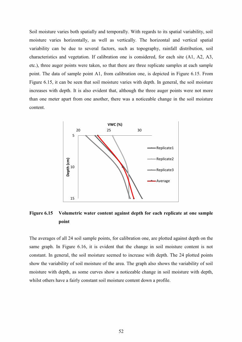
52
Soil moisture varies both spatially and temporally. With regards to its spatial variability, soil
moisture varies horizontally, as well as vertically. The horizontal and vertical spatial
variability can be due to several factors, such as topography, rainfall distribution, soil
characteristics and vegetation. If calibration one is considered, for each site (A1, A2, A3,
etc.), three auger points were taken, so that there are three replicate samples at each sample
point. The data of sample point A1, from calibration one, is depicted in Figure 6.15. From
Figure 6.15, it can be seen that soil moisture varies with depth. In general, the soil moisture
increases with depth. It is also evident that, although the three auger points were not more
than one meter apart from one another, there was a noticeable change in the soil moisture
content.
Figure 6.15 Volumetric water content against depth for each replicate at one sample
point
The averages of all 24 soil sample points, for calibration one, are plotted against depth on the
same graph. In Figure 6.16, it is evident that the change in soil moisture content is not
constant. In general, the soil moisture seemed to increase with depth. The 24 plotted points
show the variability of soil moisture of the area. The graph also shows the variability of soil
moisture with depth, as some curves show a noticeable change in soil moisture with depth,
whilst others have a fairly constant soil moisture content down a profile.
5
10
15
20 25 30
De
pth
(cm
)
VWC (%)
Replicate1
Replicate2
Replicate3
Average

53
Figure 6.16 Volumetric water content against depth for all 24 sample points
The calibration procedure was carried out once all four calibrations had been completed. The
aim of the calibration was to determine the average No value, by averaging the No value
determined for each calibration. The data from the CRP is sent, via satellite link, to the
COSMOS server: http://cosmos.hwr.arizona.edu/Probes/probemap.php. The data is available
at three levels. Level one data comprises of raw counts of fast and thermal neutrons. Level
two data is quality controlled, uses level one data and subsequently converts it into a suitable
format to determine soil moisture. Level three data takes level two data and converts it
directly to measurements of soil moisture. The calibration procedure outline that was
followed is that of Franz (2014) and Franz et al. (2015).
The first step in the calibration procedure was to correct the neutron counts. This involved
determining the neutron correction factors, using the following equations (Franz, 2014):
N = N′∗ CP ∗ CWV
CI ∗ CS (6.3)
where N is the corrected neutron counts per hour, N’ is the raw moderated neutron counts, CP
is the pressure correction factor, CWV is the water vapour correction factor, CI is the high-
energy intensity correction factor, and CS is the scaling factor for geomagnetic latitude
(Franz, 2014).
5
10
15
15 25 35 45 55
De
pth
(cm
)
VWC (%)

54
CP = exp (Pi− Po
130) (6.4)
CI = N H
i (t)
N H o (6.5)
CS = f(x, y, z, t) (6.6)
Where x, y, z, is location and elevation, and t is time.
CWV = 1 + 0.0054 (ρvi (T, P, RH) − ρv
o(T, P, RH)) (6.7)
where rvi is the absolute humidity of the air (g/m3), rv
0 is the reference absolute humidity of
the air (g/m3), T is air temperature in (oC), P is pressure (mb), and RH is relative humidity
(%) (Franz, 2014).
For the calibration procedure, the level two data was used, which has already been corrected
for CP, CI and CS. If level one data were used, then the original equation and all the
corrections are required. The revised neutron count correction equation:
𝑁 = 𝑁′ ∗ 𝐶𝑊𝑉 (6.8)
Therefore, when using level two neutron counts, only the correction for absolute water
vapour (CWV) is required. The absolute water vapour calculation was obtained, using the
following equations (Franz, 2014):
eso = 611.2 ∗ exp (17.67∗T
243.5+T) (6.9)
Where eso is the saturated vapour pressure at surface (Pa) and T is air temperature (oC)
(Franz, 2014).
eo = RH
100∗ es𝑜 (6.10)

55
Where eo is actual vapour pressure at surface (Pa) and RH is the relative humidity (%) (Franz,
2014).
ρv = eo
Rvap∗(T+273.15)∗ 1000 (6.11)
Where rv is the absolute humidity of air (g/m3), Rvap =R
0.001Mvap
is the gas constant for
water vapour (J/K/kg), R is universal gas constant (= 8.31432 J/mol/K), Mvap is the molar
mass of water vapour (= 18.01528 g/mol = 0.01801528 kg/mol ), and T is air temperature
(oC).
These equations require hourly temperature and relative humidity data for the same time
period as the level two neutron count data (hourly). The data set required covered the period
of March 2014 to March 2015. Although the CRP system does measure temperature and
pressure, the sensors are inside the data logger casing, which results in the measurement of
the loggers conditions. The primary data set used was from the eddy covariance system;
however, this only had data from the 12th of July 2014 and there were a few gaps in the data
set, which are illustrated by the vertical red arrows, as seen in Figure 6.17. This data alone
could not be used in the calibration, as the time period that it covers is not adequate and the
gaps are problematic.
Figure 6.17 Hourly temperature (The same data gaps present in the relative humidity
dataset)
0
5
10
15
20
25
30
35
3/1/2014 4/30/2014 6/29/2014 8/28/2014 10/27/2014 12/26/2014 2/24/2015
Tem
pe
ratu
re (
oC
)
Date
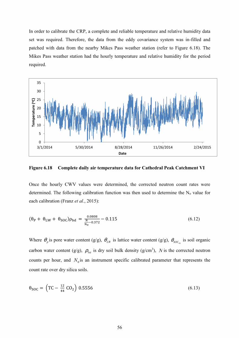
56
In order to calibrate the CRP, a complete and reliable temperature and relative humidity data
set was required. Therefore, the data from the eddy covariance system was in-filled and
patched with data from the nearby Mikes Pass weather station (refer to Figure 6.18). The
Mikes Pass weather station had the hourly temperature and relative humidity for the period
required.
Figure 6.18 Complete daily air temperature data for Cathedral Peak Catchment VI
Once the hourly CWV values were determined, the corrected neutron count rates were
determined. The following calibration function was then used to determine the No value for
each calibration (Franz et al., 2015):
(θP + θLW + θSOC)ρbd = 0.0808
N
No−0.372
− 0.115 (6.12)
Where q p is pore water content (g/g), qLW is lattice water content (g/g), qSOCeq is soil organic
carbon water content (g/g), rbd is dry soil bulk density (g/cm3), N is the corrected neutron
counts per hour, and N0 is an instrument specific calibrated parameter that represents the
count rate over dry silica soils.
θSOC = (TC − 12
44 CO2) 0.5556 (6.13)
0
5
10
15
20
25
30
35
3/1/2014 5/30/2014 8/28/2014 11/26/2014 2/24/2015
Tem
pe
ratu
re (
oC
)
Date

57
Where TC is the soil total carbon (g/g), CO2 is the soil CO2 (g/g), 12/44 represents the
stoichiometric ratio of carbon to CO2, and 0.5556 is the stoichiometric ratio of H2O to
organic carbon (assuming organic carbon is cellulose C6H10O5).
θsoc was not determined, but was given a value of 0.01 g/g.
θlw was determined to be 0.15433 g/g. A 50 gram representative soil sample was sent to
Activation Laboratories in Canada for θlw determination.
There is a need to correct for biomass (Franz et al., 2015)
(θP + θLW + θSOC)ρbd = 0.0808
N
No(BWE)−0.372
− 0.115 (6.14)
where BWE is the biomass water equivalent (mm). The biomass calculation is done for
vegetation types, whose biomass changes with their growing stage. Due to the vegetation of
Catchment VI being grassland, the biomass did not change much and the change in biomass
was therefore insignificant and a biomass correction was not required. The burning of the
catchment affected the biomass content greatly. This issue was resolved by performing a
calibration before (calibration two) and a calibration after (calibration three) the burning.
The neutron count (N) for each calibration was determined to be the average neutron count,
during which the soil samples for that calibration were obtained (Table 6.4). For the “full”
calibration, the duration was ≈ six hours. The duration of the “partial” calibration was ≈ three
hours
Table 6.4 The gravimetric soil moisture, bulk density and Neutron count
Calibration
Gravimetric Soil Moisture
(g/cm3)
Bulk density
(g/cm3)
Neutron Count
(count/hr)
1 0.490 0.593 1731.684
2 0.438 0.593 1761.408
3 0.647 0.593 1652.600
4 0.741 0.593 1611.059
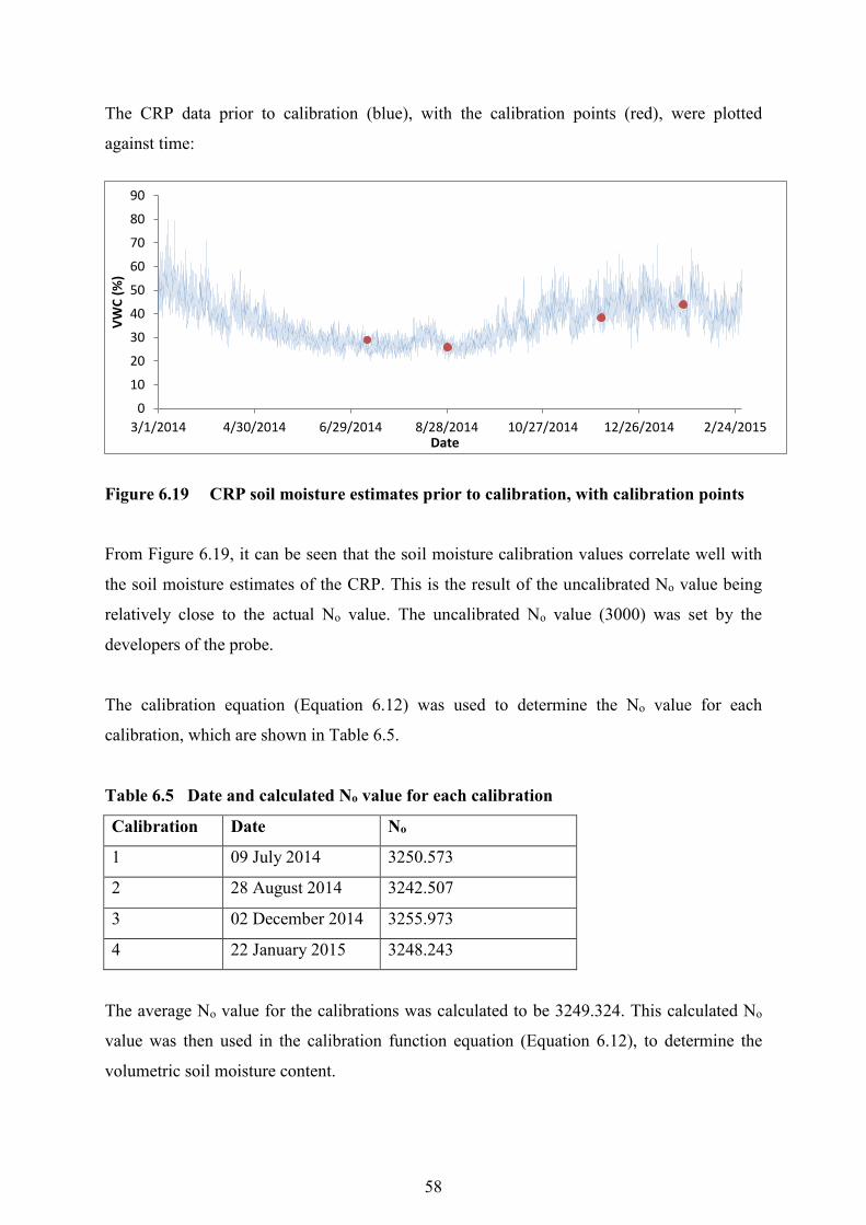
58
The CRP data prior to calibration (blue), with the calibration points (red), were plotted
against time:
Figure 6.19 CRP soil moisture estimates prior to calibration, with calibration points
From Figure 6.19, it can be seen that the soil moisture calibration values correlate well with
the soil moisture estimates of the CRP. This is the result of the uncalibrated No value being
relatively close to the actual No value. The uncalibrated No value (3000) was set by the
developers of the probe.
The calibration equation (Equation 6.12) was used to determine the No value for each
calibration, which are shown in Table 6.5.
Table 6.5 Date and calculated No value for each calibration
Calibration Date No
1 09 July 2014 3250.573
2 28 August 2014 3242.507
3 02 December 2014 3255.973
4 22 January 2015 3248.243
The average No value for the calibrations was calculated to be 3249.324. This calculated No
value was then used in the calibration function equation (Equation 6.12), to determine the
volumetric soil moisture content.
0
10
20
30
40
50
60
70
80
90
3/1/2014 4/30/2014 6/29/2014 8/28/2014 10/27/2014 12/26/2014 2/24/2015
VW
C (
%)
Date

59
The calibration function was used to determine an hourly (θp+θlw+θsoc)ρbd, by using a constant
No and the hourly corrected N values. The lattice water and soil organic carbon water
(θlw+θsoc) were subtracted from (θp+θlw+θsoc)ρbd to determine the Volumetric Water Content
(VWC) (calibrated CRP dataset). The hourly calibrated VWC from the CRP was plotted
against time, as shown in Figure 6.20.
Figure 6.20 Hourly soil moisture estimates of the calibrated CRP
From Figure 6.20, it can be seen that the calibrated hourly CRP follows the same trend as the
uncalibrated hourly CRP dataset (shown in Figure 6.24); however, there is a downward shift
in the points. The neutron count was then plotted against the calibrated VWC. The
exponential function from the graph (Figure 6.21) can be used to determine the VWC from
the neutron count measured.
Figure 6.21 Neutron count against volumetric water content
0
10
20
30
40
50
60
70
80
90
3/1/2014 4/30/2014 6/29/2014 8/28/2014 10/27/2014 12/26/2014 2/24/2015
VW
C (
%)
Date
0
10
20
30
40
50
60
70
80
90
1400 1500 1600 1700 1800 1900 2000
VW
C (
%)
Neutron (count/hr)

60
The hourly CRP data was converted into a daily dataset (Figure 6.22). From Figure 6.22, it
can be seen that the conversion from hourly to daily data results in a smoother dataset, as the
fluctuations are averaged. The soil moisture dataset generally shows that soil moisture is
higher in the summer and lower in the winter, as expected in the summer rainfall region of
South Africa.
Figure 6.22 Daily calibrated CRP soil moisture measurements in Catchment VI
6.4 Creating an In-situ Soil Moisture Dataset
There were three types/sets of in-situ soil moisture instrumentation used:
i. 5 TDR (pit) probes at one point placed horizontally at depths of 0.05, 010, 0.15, 0.20
and 0.30 m.
ii. 5 wireless TDR probes (0.12 m) placed vertically at different sites in the catchment.
iii. 8 echo probes placed horizontally at a depth of 0.10 m at different sites.
The TDR pit had the most complete data set out of all the in-situ instrument sets, as it has a
continuous record from the 11th of July 2014 to March 2015. The wireless TDR probes have
data from the 11th of July to March 2015; however, there are numerous gaps in the data set,
due to the erratic operation of all five TDR probes. The echo probes have the shortest data
record from the 9th of July 2014 to the 4th of September 2014. They were problematic and
were destroyed in a catchment fire on the 5th of September 2014.
0
10
20
30
40
50
60
3/1/2014 4/30/2014 6/29/2014 8/28/2014 10/27/2014 12/26/2014 2/24/2015
VW
C (
%)
Date
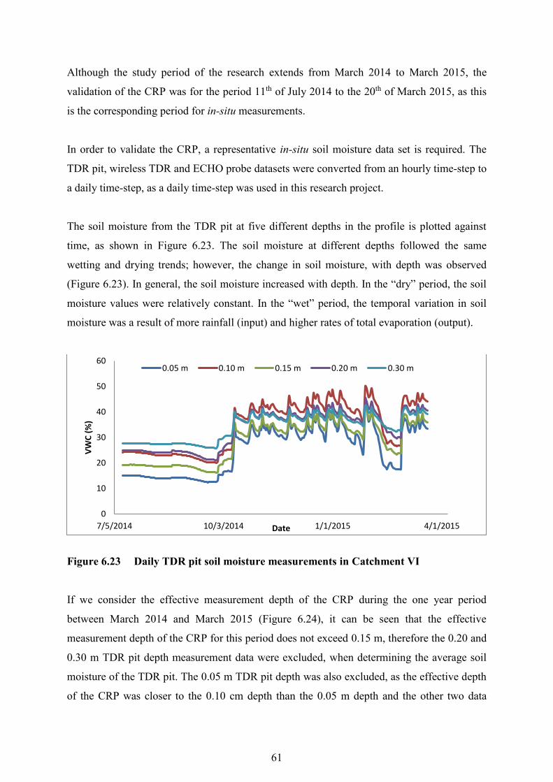
61
Although the study period of the research extends from March 2014 to March 2015, the
validation of the CRP was for the period 11th of July 2014 to the 20th of March 2015, as this
is the corresponding period for in-situ measurements.
In order to validate the CRP, a representative in-situ soil moisture data set is required. The
TDR pit, wireless TDR and ECHO probe datasets were converted from an hourly time-step to
a daily time-step, as a daily time-step was used in this research project.
The soil moisture from the TDR pit at five different depths in the profile is plotted against
time, as shown in Figure 6.23. The soil moisture at different depths followed the same
wetting and drying trends; however, the change in soil moisture, with depth was observed
(Figure 6.23). In general, the soil moisture increased with depth. In the “dry” period, the soil
moisture values were relatively constant. In the “wet” period, the temporal variation in soil
moisture was a result of more rainfall (input) and higher rates of total evaporation (output).
Figure 6.23 Daily TDR pit soil moisture measurements in Catchment VI
If we consider the effective measurement depth of the CRP during the one year period
between March 2014 and March 2015 (Figure 6.24), it can be seen that the effective
measurement depth of the CRP for this period does not exceed 0.15 m, therefore the 0.20 and
0.30 m TDR pit depth measurement data were excluded, when determining the average soil
moisture of the TDR pit. The 0.05 m TDR pit depth was also excluded, as the effective depth
of the CRP was closer to the 0.10 cm depth than the 0.05 m depth and the other two data
0
10
20
30
40
50
60
7/5/2014 10/3/2014 1/1/2015 4/1/2015
VW
C (
%)
Date
0.05 m 0.10 m 0.15 m 0.20 m 0.30 m

62
sources had measurements at 0.10 and 0.12 m depths (echo and wireless TDR). The mean
effective depth for this period was 0.11 m.
Figure 6.24 The CRP effective measurement depth
The average (0.10 and 0.15 m) daily TDR pit soil moisture was plotted against time (Figure
6.25). From Figure 6.25, it can be seen that the average TDR pit dataset covers the winter and
summer period.
Figure 6.25 The average TDR pit soil moisture measurements in Catchment VI
0.08
0.09
0.1
0.11
0.12
0.13
0.14
0.15
6/10/2014 7/30/2014 9/18/2014 11/7/2014 12/27/2014 2/15/2015 4/6/2015
De
pth
(m
)
Date
0
10
20
30
40
50
60
7/5/2014 8/24/2014 10/13/2014 12/2/2014 1/21/2015 3/12/2015
VW
C (
%)
Date

63
The daily wireless TDR data was plotted for the measurement period, as shown in Figure
6.26. The wireless TDR data has gaps in the data set. This is due to errors in the data logging
programme and faults in the sensors.
Figure 6.26 Daily wireless TDR data in Catchment VI
The Echo probe data was then plotted against time (Figure 6.27). The echo probe data only
covered the dry period, as the fire that burnt Catchment VI, also destroyed the sensors, which
could not be used again in this study.
Figure 6.27 Daily echo probe data in Catchment VI
0
10
20
30
40
50
60
7/5/2014 9/3/2014 11/2/2014 1/1/2015 3/2/2015
VW
C (
%)
Date
TDR1
TDR2
TDR3
TDR4
TDR5
0
10
20
30
40
50
60
7/5/2014 7/25/2014 8/14/2014 9/3/2014
VW
C (
%)
Date
ECHO1
ECHO2
ECHO3
ECHO4
ECHO5
ECHO6

64
All three (TDR pit, wireless TDR and echo probe) sets of data were merged by weighting
each point within the catchment equally, to create a representative in-situ soil moisture
estimate (Figure 6.28), which shows the merged dataset. This dataset weighted each sensor,
in each sample point equally.
Figure 6.28 Representative soil moisture measurements
6.5 Acquisition and Processing of the AMSR2 Soil Moisture Product
This section describes the methodology adopted to obtain the AMSR2 remote sensing soil
moisture product. The AMSR2 sensor estimates several parameters, which are predominately
linked to the energy and water cycles, namely, precipitation, water vapour, sea-surface
temperature, soil moisture and snow depth. The AMSR2 soil moisture product was obtained
from the JAXA website: http://sharaku.eorc.jaxa.jp/. The data is freely available; however, a
relatively short registration was required, in order to gain access into the GCOM-W1 Data
Providing Service.
Level Two and Level Three soil moisture data sets are available from July 2012 to present
day. The Level Two data is available on a 25 km spatial resolution grid, whilst the Level
Three data is available on both 10 km and 25 km spatial resolution grids. The Level Three
soil moisture product uses Level 1B brightness temperature and Level Two soil moisture data
and averages both of them spatially and temporally, with respect to predefined lattice grid
points on the earth’s surface.
0
10
20
30
40
50
60
7/5/2014 9/3/2014 11/2/2014 1/1/2015 3/2/2015
VW
C (
%)
Date

65
The 10 km and 25 km Level Three AMSR2 products are presented in Figure 6.29 and
illustrates the significance of spatial resolution. The 10 km spatial resolution is much finer
and therefore has a lot more detail, compared to the coarser 25 km resolution. The need for
finer spatial resolution data is to capture spatial heterogeinity and accurately represent
processes occuring at particular scales. The 10 km product results in a pixel area of 100 km2,
whilst the 25 km product results in a pixel area of 625 km2.
Figure 6.29 Comparison of spatial resolution of AMSR2 10 km and 25 km Level
Three soil moisture products
The Level Three soil moisture product at a 10 km spatial resolution was selected to be used in
this study. Once the Level Three 10 km soil moisture product is selected, the data type and
observation period needs to be specified, before specifying the search area. Once all the
specifications have been made, the data can be searched for and subsequently downloaded.
The data format is then specified and there is an option to leave the data in its original format
or convert it to HDF5, Geotiff of NetCDF. The conversion to Geotiff was chosen, as this data
format is compatible with ArcGis 9.3.
AMSR2 Level Three, 10km AMSR2 Level Three, 25km

66
The data can now be ordered. Once ordered, an order acceptance email, which contains an ftp
and URL site link to directly download the data. The data was then opened in ArcGis 9.3.
The data was defined on the WGS 84 geographic coordinate system and no projection or
transformation was required. There were two files per day, as each day had an ascending and
descending orbit.
Due to the nature of satellite orbits, on some days, the catchment area was covered by:
i. An ascending orbit;
ii. A descending orbit;
iii. An ascending and descending orbit;
iv. Neither.
The catchment shape file was overlaid onto the AMSR2 soil moisture raster image, as seen in
Figure 6.30. The pixel value that was covered by the catchment was determined. The pixel
values ranged from 0 to 600. The pixel values were multiplied by a scaling factor of 0.001, to
obtain the soil moisture in g/cm3. The density of water is assumed to be 1.0 g/cm3 and the
volume of 1.0 g of water is 1.0 cm3. Therefore, the VWC in percentage was obtained by
multiplying the scaled pixel value by 100.
Figure 6.30 The Catchment VI shapefile overlaid over the AMSR2 soil moisture
product to obtain the volumetric water content
Catchment VI
Pixel Value

67
6.6 Acquisition and Processing of the SMOS Soil Moisture Product
This section describes the methodology adopted to obtain the SMOS remote sensing soil
moisture product. Level Two and Level Three SMOS soil moisture products are available.
The Level Two soil moisture products are at a 30-50 km spatial resolution and can be
obtained from the ESA website: http://eopi.esa.int/. The data is freely available from the Eoli-
sa catalogue. The Eoli-sa catalogue gives users access to European Space Agency (ESA)
Earth Observation data products.
The Level Three SMOS soil moisture products are available from the national French and
Spanish processing entities, namely, the CATDS (Centre Aval de Traitement des Donnees
SMOS) and SMOS CP34-BEC (SMOS Barcelona Expert Centre). The BEC-34 was used, as
it was more user-friendly and the site was a lot easier to navigate. The BEC is an ESA expert
support laboratory committed to the ongoing analysis and development of new algorithms to
improve the baseline SMOS Level Two products.
The SMOS Level Three soil moisture products are computed from Level Two soil moisture
user data products, which consist of geophysical parameters, a theoretical estimate of
accuracy, flags and product descriptors. First, the Level Two soil moisture user data products
are filtered and combined into maps with the same spatial resolution. Next, the quality flags
and product descriptors are used to discard unreliable soil moisture values. The final soil
moisture product is a global daily soil moisture map on a 25 km spatial resolution grid.
The Level Three SMOS BEC-34 data was obtained from http://cp34-bec.cmima.csic.es/. This
site is the SMOS-BEC data distribution and visualization service. A short registration
procedure is required before the data can be accessed from the site’s THREDDS service,
which provides netCDF data files. The SMOS soil moisture products fall under the Land
category. The BEC land near real-time (0.25 x 0.25 degree resolution) was selected, as the
other two options had fine resolution soil moisture, which only covered the Iberian Peninsula.
The option selected was a global dataset. There are numerous soil moisture products at
different intervals. The one-day global soil moisture product was chosen. For each day, there
are two files, the ascending and descending orbits. Figure 6.31 shows the navigation through
the THREDDS service.

68
Figure 6.31 Navigation through the THREDDS service
The soil moisture product files can either be directly downloaded or viewed, using one of the
data viewers on the site. The viewers include NetCDF-Java ToolsUI, Integrated Data Viewer
and the Godiva2 online tool. The Godiva2 online visualization tool was used to obtain the
soil moisture data (Figure 7.32).

69
Figure 6.32 Layout of the Godiva2 online visualization tool
The Godiva2 visualization tool is very user-friendly and the data was easily obtained. The
required data set was viewed by selecting the necessary data requirements (1). The data
requirements were selected as follows; the BEC research products land, near-real time global
maps, daily one-day maps, choose between ascending and descending (both are required, but
are obtained separately) and lastly soil moisture (SM).
Next, the date was specified (2). The data for a specific day is viewed by clicking on the date
on the calendar. The transition from day-to-day is quick.
The global map was used to locate the co-ordinates of the area required. The correct pixel
was located, which corresponded to the co-ordinates of the catchment. The pixel information,
which consisted of its longitude, latitude and soil moisture value, was displayed (3).
A check was done to determine if the catchment was contained in one pixel. This was done
by opening the image in Google Earth (4).
1
2
3
4

70
Once it was determined that the catchment was completely contained in one pixel (Figure
6.33), the soil moisture data could be obtained by changing the date and obtaining the data by
clicking on the corresponding pixel (Figure 6.34).
Figure 6.33 The position of the catchment in relation to a single pixel of the SMOS
soil moisture product

71
Figure 6.34 Godiva2 visualization tool showing the pixel value for the Catchment VI
This method of obtaining daily soil moisture data was efficient, as the data did not have to be
downloaded, stored, opened with the appropriate software, spatially defined and projected,
before overlaying the catchment shapefile and determining the soil moisture estimate. This
online viewer was more than adequate to obtain the daily soil moisture data for both
ascending and descending data sets for a one year period. The images obtained were near-real
time, as the present day data was available the following day. The pixel values were in
volumetric water content, so no conversion was required.
6.7 Analysis of AMSR2 and SMOS Remote Sensing Data
The AMSR2 and SMOS products are daily soil moisture products; however, there were days
in which the study area was not covered by an ascending or descending orbit (missing data).
Of the 365 day study period the various days in terms of coverage are presented in Figures
6.35 and 6.36.
From Figure 6.35, it can be seen that AMSR2 data was available for 343 days of the 365
days. There were 22 days which had no data, resulting in a daily annual coverage of 94%.
The days with missing data seemed to follow a general pattern throughout the year, as there
were similar amounts of missing data each month of the observation period.
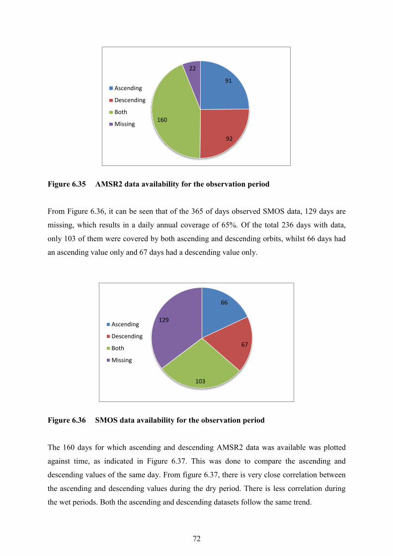
72
Figure 6.35 AMSR2 data availability for the observation period
From Figure 6.36, it can be seen that of the 365 of days observed SMOS data, 129 days are
missing, which results in a daily annual coverage of 65%. Of the total 236 days with data,
only 103 of them were covered by both ascending and descending orbits, whilst 66 days had
an ascending value only and 67 days had a descending value only.
Figure 6.36 SMOS data availability for the observation period
The 160 days for which ascending and descending AMSR2 data was available was plotted
against time, as indicated in Figure 6.37. This was done to compare the ascending and
descending values of the same day. From figure 6.37, there is very close correlation between
the ascending and descending values during the dry period. There is less correlation during
the wet periods. Both the ascending and descending datasets follow the same trend.
91
92
160
22
Ascending
Descending
Both
Missing
66
67
103
129Ascending
Descending
Both
Missing

73
Figure 6.37 Time series analysis of days which have both ascending and descending
AMSR2 values
The 103 days for which ascending and descending SMOS data was available was plotted as a
time series (Figure 6.38). From figure 6.38, it is evident that both the ascending and
descending data follow the same trend. There are differences in values between the two
datasets on the same day. These differences are larger in the wetter periods. The differences
in ascending and descending values are greater for the SMOS dataset compared to the
AMSR2 dataset.
Figure 6.38 Time series analysis of days which have both ascending and descending
SMOS values.
0
5
10
15
20
25
30
35
40
45
50
3/1/2014 4/20/2014 6/9/2014 7/29/2014 9/17/2014 11/6/2014 12/26/2014 2/14/2015 4/5/2015
VW
C (
%)
Date
Ascending Descending
0
10
20
30
40
50
60
70
3/1/2014 4/30/2014 6/29/2014 8/28/2014 10/27/2014 12/26/2014 2/24/2015
VW
C (
%)
Date
Ascending Descending

74
The differences observed between the ascending and descending values for the same day and
over the time period can be attributed to the temporal variation in soil moisture. The
ascending values are obtained at 06:00, whereas the descending values are obtained at 18:00.
Therefore, the change in soil moisture during this 12-hour interval could be due to rainfall
and total evaporation.
This is further emphasized in the dry period, when rainfall and total evaporation is low. The
ascending and descending values correlate well, as the VWC does not change much in the
interval. However, in summer, the rainfall and total evaporation rates are high resulting in
changes in the VWC between the ascending and descending measurements.
There are expected differences between ascending and descending overpass soil moisture
retrievals, due to the difference in geophysical conditions at day time and night time, with
night time conditions being more favourable for soil moisture retrieval (Kim et al., 2015).
Therefore, should soil moisture studies only use descending values, which would result in
more missing data days, but better favourable soil moisture retrieval values.
An alternative is to use only the days which have both ascending and descending values, as
this will average the two retrieval values, however, there will also be a large number of
missing data days. For this research study, all observation days with ascending, descending
and days with both ascending and descending values were used.
6.8 PyTOPKAPI Soil Moisture Product (SAHG)
This section details the acquisition of the PyTOPKAPI modeled soil moisture estimates. The
PyTOPKAPI soil moisture product was obtained from the Satellite Applications and
Hydrology Group (SAHG) website: http://sahg.ukzn.ac.za/.
The PyTOPKAPI modelled soil moisture product will be referred to as the SAHG soil
moisture product. The soil moisture products are freely and readily available. The data has a
temporal resolution of three hours and is on a spatial resolution grid ≈ 12.5 km. The data
ranges from the year 2008 to the present.

75
The data was obtained by downloading the SSI (soil saturation index) product in the ascii file
format, which can be opened and processed in ArcGis 9, as seen in Figure 6.39. The soil
moisture data for each day was available on a three-hour time-step. Therefore, eight files had
to be downloaded for each day.
Figure 6.39 Navigation through the SAHG website to download SSI data
The files were then opened in ArcGis 9.3 and the spatial referencing of the data was first
checked. The data was defined in the correct spatial reference (WGS 84 geographic co-
ordinates) and no defining projections and transformations were required. The soil moisture
products were on a three-hour time-step: (i) 00:00, (ii) 03:00, (iii) 06:00, (iv) 09:00, (v)
12:00, (vi) 15:00, (vii) 18:00 and (viii) 21:00 (see Figure 6.40). These eight raster images per
day had to be converted into a daily raster image. This was done by using the Mosaic to New
Raster option under the Data Management Tools in ArcGIS 9.3.

76
Figure 6.40 One day of SSI data (eight images on a three hour interval)
Once the daily image was created (Figure 6.41), the catchment shape file was overlaid onto it
(Figure 6.42). The pixel value was then determined and recorded.

77
Figure 6.41 Daily SAHG soil moisture product
Figure 6.42 Overlay of the Cathedral Peak Catchment VI onto the SAHG soil
moisture product

78
The soil moisture data from the SAHG product is represented as a soil saturation index (SSI),
which is expressed as a percentage. The SSI was then converted into a VWC, using the
simplified equation.
𝑆𝑆𝐼 = 𝑉𝑊𝐶
𝑃𝑜𝑟𝑜𝑠𝑖𝑡𝑦 (6.15)
The SSI equation (Equation 6.15) can easily be rearranged to solve for VWC:
𝑉𝑊𝐶 = 𝑆𝑆𝐼 × 𝑃𝑜𝑟𝑜𝑠𝑖𝑡𝑦 (6.16)
The soil porosity can be determined by measurement or calculation. In order to calculate
porosity, the following equation was used:
𝑃𝑜𝑟𝑜𝑠𝑖𝑡𝑦 = 1 − 𝑃𝑏
𝑃𝑠 (6.17)
where Pb is the bulk density and Ps is the particle density. The bulk density was determined
to be 0.593 g/cm3 and a generic value of 2.65 g/cm3 was used for the particle density (Hillel,
2008).
𝑃𝑜𝑟𝑜𝑠𝑖𝑡𝑦 = 1 − 0.593
2.65
The porosity was calculated to be 0.77. Therefore, from Equation 6.16, all the SSI values
were multiplied by 0.77, to convert them to volumetric water content.
The porosity was determined from the bulk density, which was valid for the top 0.15 m of the
soil surface. The PyTOPKAPI soil moisture product is the SSI for the A and B horizon of the
soil profile. Therefore, a porosity value that represents the A and B (one meter depth)
horizon, needs to be determined. A study conducted by Everson et al. (1998), contains soil
bulk density values for Catchment VI at depths of 0.20, 0.50, 0.75 and 1.00 m (Table 6.6).
The bulk density values used in this study can be incorporated and used to obtain a
representative porosity value that covers the A and B horizons. The porosity values should
not have changed over the past 16 years, as the catchment is in a protected area.

79
Table 6.6 The bulk density of Catchment VI, as determined by Everson et al. (1998)
Soil Depth (m) Dry Season Wet Season Mean 0.20 0.660 0.786 0.868 0.886 0.800 0.50 0.898 0.899 0.847 0.798 0.861 0.75 0.803 0.757 0.662 0.784 0.752 1.00 0.863 0.799 0.905 0.844 0.853
These bulk density values were incorporated into the values that were obtained in this study
and the mean bulk density of the soil profile (0 to 1.00 m) was determined (Table 6.7).
Table 6.7 Mean bulk density according to depth
Soil Depth (m) Mean Bulk density (g/cm3) 0.05 0.525 0.10 0.597 0.15 0.656 0.20 0.800 0.50 0.861 0.75 0.752 1.00 0.853 Average 0.720
The average bulk density was 0.720 g/cm3. The average porosity was calculated, using the
new bulk density value in Equation 6.12.
𝑃𝑜𝑟𝑜𝑠𝑖𝑡𝑦 = 1 − 0.720
2.65 (6.12)
The average porosity is 0.728. Therefore, the SSI pixel values obtained must be multiplied by
0.728, in order to convert them into VWC (Equation 6.11).

80
6.9 Surface Energy Balance System (SEBS)
The SEBS Model, developed by Su (2002), was run in the Integrated Land and Water
Information System (ILWIS) 3.8.3 for the estimation of relative evaporation and evaporative
fraction in Cathedral Peak Research Catchment VI for the period of March 2014 to March
2015. The SEBS Model uses remote sensing and meteorological data sets to estimate heat
fluxes.
Landsat 8 images were used for the estimation of relative evaporation and evaporative
fraction, using the SEBS Model. The Landsat 8 satellite, as seen in Figure 6.43, is the latest
addition to the Landsat series and was launched on the 11th of February 2013 (Markham et
al., 2015). Landsat satellites have continuously acquired information of the earth’s land
surface since 1972, thus the continuation of data acquisition from the Landsat 8 satellite is
essential (USGS, 2013). Landsat 8 orbits the earth at an altitude of 705 km, which results in
14 full orbits being completed each day, with every point of the earth being covered once
every 16 days. The satellite carries out north to south orbits and has an overpass time of 10:00
(Markham et al., 2015). Landsat 8 carries two push-broom sensors, so that the reflective and
thermal bands were split into two instruments (Markham et al., 2015). These two instruments
are the Operational Land Imager (OLI) and Thermal Infrared Sensor (TIRS).
Figure 6.43 Landsat 8 satellite

81
Landsat 8 images were used in this study due to their spatial resolution. It has the ability to
estimate relative evaporation and evaporative fraction at a spatial resolution of 30 m,
however, it has a temporal resolution of 16 days. The Landsat 8 product consists of several
bands (one to eleven), each band having its own spectral characteristics and wavelength range
(Table 6.8).
Table 6.8 Characteristics of the various landsat 8 bands (USGS, 2015).
Spectral bands Wavelength (μm) Resolution (m) 1- coastal/aerosol 0.43-0.45 30 2- blue 0.45-0.51 30 3- green 0.53-0.59 30 4- red 0.64-0.67 30 5- near IR 0.85-0.88 30 6- SWIR 1 1.57-1.65 30 7- SWIR-1 2.11-2.29 30 8- panchromatic 0.50-0.68 15 9- cirrus 1.36-1.38 30 10- TIRS 1 10.60-11.19 100 11- TIRS 2 11.50-12.51 100
Landsat 8 satellite imagery was freely acquired from the Earth Explorer website:
http://earthexplorer.usgs.gov. The area of interest and time period of the data required was
specified. Next, the data set that the user requires can be selected from a list of all the
available data sets. The data set selected was the L8 OLI/TIRS. The catchment study area fell
within one Landsat 8 image. The Landsat 8 image footprint is very large, as seen in Figure
6.44. Between March 2014 and March 2015, there were a total of 22 images.
Figure 6.44 Landsat 8 image footprint

82
Most of the images, which were acquired, were for clear sky conditions. Some images
possessed variable cloud cover; however, the area of interest was cloud-free, therefore, the
image could still be used. There were six images, which could not be used for the retrieval of
the evaporative fraction and relative evaporation, as the image contained cloud cover, which
blocked the area of interest. The different cloud-cover conditions are seen in Figure 6.45.
Figure 6.45 Landsat images with different cloud-cover conditions
Of the 22 images available for the study period, only 16 images could be used due to cloud-
cover. The 16 images that could be used were downloaded. The Level one Geotiff Data
Product was the download option selected. Each Level One Geotiff product contains a
Material Library (MTL) file, which contains all the necessary information (metadata) about
the images and 12 images, which include images B1 to B11 and BQA, where B1 is band one
and B11 is band eleven.

83
The ILWIS 3.8.3 software was downloaded from http://52north.org/downloads/ilwis/. The
images (bands) were imported into ILWIS 3.8.3 as digital numbers (DN). The bands required
were 2, 3, 4, 5, 6, 7, 10 and 11. These bands were rescaled to Top of Atmosphere (TOA)
reflectance and/or radiance, using the radiometric rescaling coefficients provided in the
metadata file. The procedure followed has been outlined by Allen et al. (2002) and the USGS
(2015). The USGS (2015) provides the necessary equations for the conversion to TOA
Radiance, conversion to TOA Reflectance and conversion to TOA brightness temperature.
The equations to obtain the inputs into the SEBS Model, such as the albedo, NDVI, surface
emissivity and land surface temperature maps are presented in Allen et al. (2002). Although
the equations in Allen et al. (2002) were intended to be used in SEBAL, they can be used in
other models, such as SEBS.
Conversion to TOA Radiance
Bands 10 and 11 (TIRS bands) were converted to TOA Radiance, using the radiance
rescaling factors provided in the metadata file (USGS, 2015).
Lλ = (𝑀𝐿 ∗ 𝑄𝑐𝑎𝑙) + 𝐴𝐿 (6.18)
where, Lλ is the TOA spectral radiance (Watts/(m2*srad*µm)), ML is the band specific
multiplicative rescaling factor (RADIANCE_MULT_BAND_X) from the metadata file
(where X is the band number), Qcal is the quantized and calibrated standard product pixel
value (DN) and AL is the band specific additive rescaling factor
(RADIANCE_ADD_BAND_X) from the metadata (where X is the band number).
Conversion to TOA Reflectance
Bands 2, 3, 4, 5, 6 and 7 (OLI bands) were converted to TOA planetary reflectance, using
reflectance rescaling coefficients provided in the metadata file (USGS, 2015).
Pλ′ = (𝑀𝑃 ∗ 𝑄𝑐𝑎𝑙) + 𝐴𝑃 (6.19)

84
where Pλ′ is the TOA planetary reflectance (without solar angle correction), Mp is the band
specific multiplicative reflectance factor (REFLECTANCE_MULT_BAND_X) from the
metadata file (where X is the band number) and Ap is the band specific additive rescaling
factor (REFLECTANCE_ADD_BAND_X) from the metadata (where X is the band number).
The TOA reflectance was then corrected for the sun angle (USGS, 2015):
Pλ =Pλ′
sin (Θ𝑆𝐸) (6.20)
where pλ is the TOA planetary reflectance and ΘSE is the local sun elevation
(SUN_ELEVATION), which is obtained from the metadata file.
The ESUN values were determined for bands 2, 3, 4, 5, 6 and 7, using the following
equations (Allen et al., 2002):
𝐸𝑆𝑈𝑁 = (𝜋 ∗ 𝑑2) ∗ (𝑅𝐴𝐷_𝑀𝐴𝑋
𝑅𝐸𝐹_𝑀𝐴𝑋) (6.21)
Where d is the earth-sun distance, RAD_MAX is the maximum radiance and REF_MAX is
the maximum reflectance (all of which are found in the metadata file).
The ESUN values (Table 6.9) are required to create an equation to determine albedo for the
TOA (Allen et al., 2002).
𝛼𝑇𝑂𝐴= ∑(𝜔λ ∗ Pλ) (6.22)
𝜔λ =𝐸𝑆𝑈𝑁λ
∑𝐸𝑆𝑈𝑁λ (6.23)
Table 6.9 Calculated ESUN values
Band ωλ Band ωλ 2 0.300 5 0.143 3 0.277 6 0.036 4 0.233 7 0.012

85
The ESUN band values change, due to changes in the earth-sun distance (d), maximum
radiance and maximum reflectance of each data product. However, the 𝜔λ band value was
determined to be the same for each image, as the ratio remains the same.
Albedo is then calculated by correcting TOA albedo, using the following equation (Allen et
al., 2002):
∝=𝛼𝑇𝑂𝐴−𝛼𝑃𝑎𝑡ℎ_𝑟𝑎𝑑𝑖𝑎𝑛𝑐𝑒
𝜏𝑠𝑤2 (6.24)
where αPath_radiance is 0.03 and τsw is 0.774 (Allen et al., 2002).
The generated albedo map is illustrated in Figure 6.46. Albedo ranges from 0.0 to 1.0 and is a
measure of the reflectivity of the earth’s surface. As the reflectivity increases, the albedo
value increases. Grasslands generally have an albedo of between 0.15 to 0.25.
Figure 6.46 Albedo map generated in ILWIS
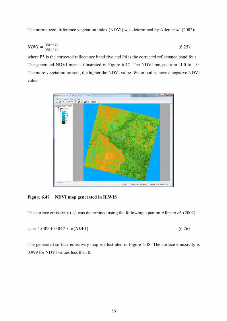
86
The normalized difference vegetation index (NDVI) was determined by Allen et al. (2002):
𝑁𝐷𝑉𝐼 =(𝑃5−𝑃4)
(𝑃5+𝑃4) (6.25)
where P5 is the corrected reflectance band five and P4 is the corrected reflectance band four.
The generated NDVI map is illustrated in Figure 6.47. The NDVI ranges from -1.0 to 1.0.
The more vegetation present, the higher the NDVI value. Water bodies have a negative NDVI
value.
Figure 6.47 NDVI map generated in ILWIS
The surface emissivity (εo) was determined using the following equation Allen et al. (2002):
𝜀𝑜 = 1.009 + 0.047 ∗ ln (𝑁𝐷𝑉𝐼) (6.26)
The generated surface emissivity map is illustrated in Figure 6.48. The surface emissivity is
0.999 for NDVI values less than 0.

87
Figure 6.48 Surface emissivity map generated in ILWIS
The TIRS bands (bands 10 and 11) are converted from spectral radiance to at-satellite
brightness temperature, using the following equation (USGS, 2015):
𝑇𝑏𝑏 = 𝐾2
𝑙𝑛[𝐾1
𝐿λ+1]
(6.27)
Where K1 and K2 are constants, which are found in the metadata file and Lλ is either band
10 or band 11, according to high or low gain conditions. Band 11 was used in this study, as
high gain is suited for grassland vegetation.
The Land Surface Temperature (LST) can be determined by Allen et al. (2002):
𝐿𝑆𝑇 = 𝑇𝑏𝑏
𝜀𝑜0.25 (6.28)
Figure 6.49 shows the generated land surface temperature map. The land surface temperature
is expressed in degrees kelvin.

88
Figure 6.49 Land surface temperature map generated in ILWIS
The SEBS Model requires a digital elevation model (DEM) (Figure 6.50), as input. The DEM
of South Africa was obtained http://srtm.csi.cgiar.org. The DEM for each image had to be
resampled before it could be used:
Figure 6.50 DEM map used in ILWIS as an input in SEBS

89
Once the input maps (albedo, NDVI, surface emissivity, land surface temperature and DEM)
had been created, the SEBS Model was run in ILWIS. The meteorological data required to
run the model was obtained from the eddy covariance weather data, which is located within
Catchment VI. On the days where the eddy covariance weather data was not available, data
from the nearby Mikes Pass weather station was used. The data required from the weather
station were the instantaneous downward solar radiations, wind speed, air temperature,
pressure, mean daily air temperature and sunshine hours. The downward solar radiation, wind
speed, air temperature and pressure data were at the time of the satellite overpass (10:00 am).
Figure 6.51 The SEBS model in ILWIS
The SEBS Model was run (Figure 6.51) and many outputs were generated. These outputs
included daily evaporation, relative evaporation, evaporative fraction, net radiation, soil heat
flux, sensible heat flux dry, sensible heat flux wet, sensible heat flux index and leaf area
index.

90
For the purpose of this research, the evaporative fraction (Figure 6.52) and relative
evaporation (Figure 6.53) outputs were required.
Figure 6.52 Evaporative fraction map generated as an output of the SEBS model in
ILWIS
Figure 6.53 Relative evaporation map generated as an output of the SEBS model in
ILWIS

91
The relative evaporation output map (Figure 6.53) was exported as in ASCII format. The
output ASCII file was opened in ArcGIS 9.3 (Figure 6.54). The spatial reference of the
relative evaporation map was defined as WGS 1984 UTM Zone 35 N. The catchment
shapefile was projected to WGS 1984 UTM Zone 35 N and overlaid onto the relative
evaporation map (Figure 6.55).
Figure 6.54 Catchment VI shapefile overlaid onto relative evaporation map
Figure 6.55 The relative evaporation map of Catchment VI
Catchment VI
Catchment VI

92
The spatial analyst tool was then used in ArcGIS 9.3 data management tools, to calculate the
zonal statistics of the area enclosed by the catchment shapefile. Table 6.10 shows the zonal
statistics, it can be seen that the catchment encloses 686 pixels. The mean value is taken from
the zonal statistics as the relative evaporation for that image. The same procedure was
repeated to determine the evaporative fraction values.
Table 6.10 Zonal statistics of relative evaporation enclosed by catchment VI
Once the relative evaporation and evaporative fraction values had been determined, soil
moisture was calculated, using two equations, one by Su et al. (2003) (Equation 4.13) and the
other by Scott et al. (2003) (Equation 4.14).
The SEBS process is depicted in the flow diagram (Figure 6.56). It illustrates the various
procedures required to obtain relative evaporation and the evaporative fraction, using the
SEBS model.

93
Figure 6.56 Processes used to obtain relative evaporation from Landsat 8 data
Import
Bands 2
,3,4
,5,6
,7,1
0 a
nd 1
1
as D
igital
num
bers
(D
N)
in Ilw
is
Convers
ion to T
OA
Reflecata
nce
(Bands 2
,3,4
,5,6
and 7
)
Pλ′=
(𝑀𝑃∗𝑄
)+
𝐴𝑃
Sun a
ngle
corr
ection
Pλ=
Pλ′
sin(Θ
𝑆𝐸)
TO
A a
lbedo
𝛼𝑇 𝐴= ∑
(𝜔λ ∗ Pλ)
Alb
edo
∝=
𝛼𝑇 𝐴−
𝛼𝑃 𝑡
_𝑟 𝑑𝑖
𝑠
2
ND
VI
𝑁𝐷𝑉𝐼=
(𝑃5−
𝑃4)
(𝑃5+
𝑃4)
Convers
ion to T
OA
Radia
nce
(Bands 1
0 a
nd 1
1)
Lλ=
(𝑀
𝐿∗𝑄
)+
𝐴𝐿
Brightn
ess T
em
pera
ture
𝑇𝑏𝑏=
2
1
𝐿λ+
1
Land s
urf
ace tem
pera
ture
𝑇𝑆=
𝑇𝑏𝑏
𝜀𝑜0.25
Surf
ace e
mis
siv
ity
𝜀𝑜=
1.009+
0.047∗ln(𝑁
𝐷𝑉𝐼)
SEB
S
ILW
IS 3.8
.3
Mete
oro
logic
al D
ata
Sola
r ra
dia
tion
Win
dspeed
Tem
pera
ture
Pre
ssure
Sunshin
e h
ours
Avera
ge tem
pera
ture
DEM
Sun
zenith
angle
Julia
n d
ay

94
7. RESULTS AND DISCUSSION
This chapter presents the results and discussion of the various aspects of the research project.
The section will detail the following aspects:
i. The validation of the CRP with a representative in-situ soil moisture data set;
ii. The validation of remote sensing soil moisture products (AMSR2 and SMOS) with
CRP soil moisture estimates; and
iii. The validation of modelled soil moisture products (SAHG and SEBS) with CRP soil
moisture estimates.
The term validation is used in the sense of an assessment, rather than a strict justification to
observations. The validation will therefore focus on the comparison of spatial pattern,
temporal development and regularity (consistency of estimates produced) amongst the
different data sources. The types of analyses implemented in this research study include:
i. Time series analysis;
ii. Correlation coefficient (R) and coefficient of determination (R2);
a. The slope of the graph represents the change in y-units per change in x-units
(the change of variable two to the change in variable one). The closer the slope
value is to 1, the better the datasets correlate to one another;
b. R2 is the coefficient of determination and denotes the strength of the linear
association between variable x and variable y. R2 ranges from zero to one (0≤
R2 ≤ 1). The strength of the linear association increase as R2 becomes closer to
one;
iii. Residual analysis; and
iv. Paired t-test.
The statistical analyses selected for this study are amongst the most common analyses used in
current satellite-based soil moisture studies. These analyses are considered appropriate to
validate the various soil moisture products used in this study, in order to draw reliable
conclusions. The above statistical analyses, will not all be used on each validation, but will be
selected for use appropriately.

95
Soil moisture varies both spatially and temporally and fluxes in soil moisture content occur
over short time periods. The key input to soil moisture content is rainfall. Therefore, rainfall
data is necessary to describe and supplement changes in soil moisture. Rainfall data from a
rain gauge situated within Catchment VI was obtained for the one year period from March
2014 to March 2015 on an event basis. This data was then converted to a daily rainfall
dataset, as shown in Figure 7.1. The rainfall distribution shows that the majority of the
rainfall occurs in the summer months. During winter there are a few small rainfall events,
whilst in summer there are several rainfall events, which vary in magnitude.
Figure 7.1 Daily rainfall measured at Catchment VI
7.1 Validating the CRP
One of the key objectives of this research project is to test the suitability of the CRP for
providing spatial estimates of soil moisture. In order to achieve this, the CRP is validated
against a representative in-situ soil moisture data set.
A time series analysis was plotted to visually interpret and compare the CRP dataset and the
representative in-situ data set (Figure 7.2). Although the study period of the research project
was from the 1st of March 2014 to the 28th of February 2015 (one year), the time period in
which the representative data set was available (12th July 2014 to 28th February 2015) was
0
10
20
30
40
50
60
70
80
90
100
3/1/2014 5/1/2014 7/1/2014 9/1/2014 11/1/2014 1/1/2015
Rai
nfa
ll (m
m)
Date

96
used. This time period is considered adequate for the validation procedure, as both the wet
(summer) and dry (winter) periods are covered.
As shown in Figure 7.2, the CRP estimates followed the same seasonal trend as the in-situ
soil moisture data set. The CRP estimates correlated to the in-situ soil moisture data set better
in the wetter periods, when the soil moisture values were higher (above 30%), compared to
the drier periods. The CRP soil moisture estimates were higher than the in-situ estimates for
the dry period with low VWC values. This could be due to the differences in the
measurement depths between the CRP and the representative in-situ instruments. Overall, it
can be seen that the CRP dataset followed the general trend of the in-situ soil moisture
variations. The soil moisture fluctuations were dependent on the rainfall input and total
evaporation rate, as there were smaller fluctuations in winter, due to less rainfall and a lower
total evaporation rate. In summer, the fluctuations in soil moisture were greater, due to more
rainfall and a higher rate of total evaporation. There were differences between the datasets, as
the CRP dataset was generally slightly higher than the in-situ dataset. This difference was
more noticable when the soil moisture content was low. Overall, the CRP data seemed to
correlate well with the in-situ soil moisture dataset.
Figure 7.2 Daily in-situ and CRP soil moisture estimates for Catchment VI
A graph of correlation coefficients was then plotted with the representative in-situ data set on
the x-axis and the CRP estimates on the y-axis (Figure 7.3). From Figure 7.3, it can be seen
0
10
20
30
40
50
60
0
10
20
30
40
50
60
70
80
90
100
7/11/2014 9/11/2014 11/11/2014 1/11/2015
VW
C (
%)
Rai
nfa
ll (m
m)
Date
Rainfall In-situ CRP

97
that the majority of the points are above the 1:1 line (red), however they are in close
proximity to the 1:1 line. There seems to be no extreme outliers. The positive y-intercept of
12.024 indicates an over-estimation by the CRP of the lower values (when the soil is drier).
The slope is 0.709, which represents the relationship between the variables, with respect to
their increases and decreases. This indicates that there is a good correlation between both data
sets, as the value is close to 1. The R2 is 0.845. It is a measure of the strength of the linear
association between the datasets.
Figure 7.3 Scatterplot of In-situ soil moisture estimates against CRP estimates
A graph of the residuals was then plotted (Figure 7.4). The ∆ VWC (%) was the difference
between the in-situ (independent) and CRP (dependent) datasets. This graph is plotted to
illustrate how the difference in variables change over time. From Figure 7.4, it can be seen
that the majority of the residuals are negative, which indicates that the CRP soil moisture
values are higher than those of the subsequent representative in-situ values. When the soil
moisture content is high in the wet period, the residuals are lower in absolute value, which
indicates less of a difference between the data sets. The residuals are negative in the dry
periods and they also have the highest absolute value. In the wet periods, the residuals are
lower and are mostly negative; however, there are some positive values.
y = 0.7099x + 12.024R² = 0.8445
0
10
20
30
40
50
0 10 20 30 40 50
CR
P (
WC
(%
)
In-situ VWC (%)

98
Figure 7.4 Residual graph of In-situ against CRP soil moisture estimates
A paired T-test was then conducted on the two data sets (Table 7.1). This analysis indicates
whether the datasets were significantly different to each other. From Table 7.1, it can be seen
that the mean of the CRP is greater than that of the in-situ dataset, which results in the t-stat
value being negative. The variance, which is the average of the squared differences from the
mean, is the standard deviation squared. There are 436 degrees of freedom (df). The absolute
value of the t-stat (4.827) is greater than the critical two-tail value (1.965) and the P value
(1.919x10⁻⁶) is less than the alpha value (0.05). Therefore, there is a significant difference
between the datasets.
Table 7.1 T-test of In-situ against CRP estimates
In-situ CRP Mean 29.557 33.005 Variance 74.464 44.433 Observations 233 233 Hypothesized Mean Difference 0 df 436 t Stat -4.827 P(T<=t) two-tail 1.919x10⁻⁶ t Critical two-tail 1.965
-12
-8
-4
0
4
8
12
7/11/2014 9/11/2014 11/11/2014 1/11/2015
∆ V
WC
(%)
Date

99
The inconsistencies seen in the data comparison could be due to the following. The
calibration and validation of the CRP is not a straight-forward task. The calibration of the
CRP could contain bias errors, due to the sampling points selected. If different sampling
points were chosen, the soil moisture estimates could be different.
The in-situ dataset that was used to validate the CRP was not the actual average of the
catchment, but the average of the sensors in the catchment. If the sensors were placed in
different locations in the catchment, the in-situ dataset could be different. The area covered
by the in-situ sensors was far smaller than that covered by the CRP. The in-situ soil moisture
sensors were a maximum of 200 m away from the CRP, however, the CRP has a
measurement footprint that exceeds 200 m in radius. In addition, the representative data set
was biased towards the TDR pit as it was the only continous dataset, which resulted in one
single point weighing more than any other point.
The CRP was not measuring soil moisture at a constant depth. The CRP measurement depth
was dependent on the soil moisture content. Thus, when the soil was dry, the CRP probe was
measuring at a deeper depth than when the soil was wet. The representative in-situ data set
was meassuring constantly at an average depth of about 12 cm, whilst the CRP was
measuring at around 14 cm when the soil is dry and 11 cm when the soil was wet. Therefore,
the dry periods did not correlate as well as the wet periods, as the measurement depths were
different. Overall, it can be seen that the CRP was suitable to provide spatial estimates of soil
moisture. The CRP probe data set will then be used to validate the satellite-based estimates of
soil moisture.
7.2 AMSR2 Soil Moisture Product Validation
The AMSR2 Level Three soil moisture product is on a 10 km spatial resolution grid.
Although this grid is relatively small in comparison to other remote sensing soil moisture
products, it is still very large in comparison to the catchment area. The catchment area is 0.68
km2, whilst the pixel area is 100 km2. Therefore the pixel is 147 times larger than the study
area. However, validating remote sensing soil moisture products, such as the AMSR2
product, with CRP estimates is an improvement from validating remote sensing soil moisture
products with in-situ point measurements. For this analysis, the one-year study period of the
1st of March 2014 to the 28th of February 2015 was used. A time series analysis graph was
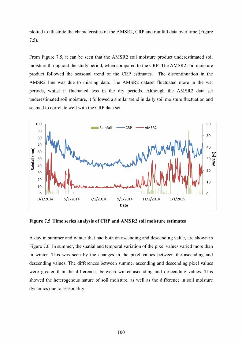
100
plotted to illustrate the characteristics of the AMSR2, CRP and rainfall data over time (Figure
7.5).
From Figure 7.5, it can be seen that the AMSR2 soil moisture product underestimated soil
moisture throughout the study period, when compared to the CRP. The AMSR2 soil moisture
product followed the seasonal trend of the CRP estimates. The discontinuation in the
AMSR2 line was due to missing data. The AMSR2 dataset fluctuated more in the wet
periods, whilst it fluctuated less in the dry periods. Although the AMSR2 data set
underestimated soil moisture, it followed a similar trend in daily soil moisture fluctuation and
seemed to correlate well with the CRP data set.
Figure 7.5 Time series analysis of CRP and AMSR2 soil moisture estimates
A day in summer and winter that had both an ascending and descending value, are shown in
Figure 7.6. In summer, the spatial and temporal variation of the pixel values varied more than
in winter. This was seen by the changes in the pixel values between the ascending and
descending values. The differences between summer ascending and descending pixel values
were greater than the differences between winter ascending and descending values. This
showed the heterogenous nature of soil moisture, as well as the difference in soil moisture
dynamics due to seasonality.
0
10
20
30
40
50
60
0
10
20
30
40
50
60
70
80
90
100
3/1/2014 5/1/2014 7/1/2014 9/1/2014 11/1/2014 1/1/2015
VW
C (
%)
Rai
nfa
ll (m
m)
Date
Rainfall CRP AMSR2

101
Figure 7.6 Comparison between summer and winter images of AMSR2 soil moisture
estimates

102
A scattergraph of CRP (x-axis ) against AMSR2 (y-axis) was then plotted (Figure 7.7). From
Figure 7.7, all the data points are below the 1:1 line (red), which shows that the AMSR2
dataset is always under-estimating soil moisture in comparison to the CRP. The slope of the
graph is 0.649, which is good. There is a positive correlation and the R2 is 0.505, which
indicates a good fit. There are some outliers above and below the line of best fit.
Figure 7.7 Scatterplot of CRP against AMSR2 soil moisture estimates
A residual graph of the CRP against AMSR2 soil moisture was then plotted against time
(Figure 7.8). The ∆ VWC (%) was the difference between the CRP and AMSR2 datasets.
From the residual graph (Figure 7.8), it can be seen that the AMSR2 dataset was under-
estimating soil moisture throughout the study period. In the dry period, the residuals were
fairly constant, whilst in the wet periods, the residuals fluctuated more. The mean residual
was 22.81. The residuals were constantly lower in the dry period, compared to the wet period,
which indicates that there was less underestimation of the AMSR2 data in the dry period.
y = 0.6492x - 11.125R² = 0.505
0
20
40
60
0 20 40 60
AM
SR2
VW
C (
%)
CRP VWC (%)

103
Figure 7.8 Residual graph of CRP against AMSR2 soil moisture estimates
A paired t-test was then conducted (Table 7.2). In order to properly perform a t-test, paired
values were required. Therefore, the CRP values corresponding to the AMSR2 days, which
had no data, were removed. From Table 7.2, it can be seen that the means are very different,
as the mean of the CRP is 33.326 and AMSR2 is 10.511. The variance values are similar, as
the variance of the CRP is 50.010 and the AMSR2 is 41.737. There are 669 degrees of
freedom. The t-stat value (43.791) exceeds the t critical value (1.964) and the P value
(1.3x10-198) is less than alpha (0.05). Therefore, there is a significant difference between the
datasets.
Table 7.2 T-test of CRP against AMSR2 estimates
CRP AMSR2 Mean 33.326 10.511 Variance 50.010 41.737 Observations 338 338 Hypothesized Mean Difference 0 df 669 t Stat 43.791 P(T<=t) two-tail 1.3x10-198 t Critical two-tail 1.964
When the AMSR2 product data was processed and the pixel values obtained, it was found
that the daily data values corresponded to four different situations. There were days when
only a descending pixel value was available (10th of December 2014) and there were days
when only an ascending pixel value was available (11th of December 2014) (Figure 7.9).
0
5
10
15
20
25
30
35
40
45
50
3/1/2014 5/1/2014 7/1/2014 9/1/2014 11/1/2014 1/1/2015
∆ V
WC
(%)
Date

104
There were days when both an ascending and descending pixel value was available (14th of
December 2014) and there were days when no pixel data was available for the catchment area
(15th of December 2014) (Figure 7.10).
Figure 7.9 A day with a descending and a day with an ascending value for the AMSR2
soil moisture product

105
Figure 7.10 A day with both an ascending and descending value, and a day with no
value for the AMSR2 soil moisture product

106
7.3 SMOS Soil Moisture Product Validation
The SMOS Level Three soil moisture product is on a 25 km spatial grid. Although this grid is
smaller than that of the Level Two product (40 km), it is still very large in comparison to the
catchment area. The catchment area is 0.68km2, whereas the pixel area is 625km2. Therefore,
the pixel is 920 times larger than the study area.
A graph of the time series analysis of the daily CRP and SMOS datasets were plotted (Figure
7.11). The time period used, was a one year period from the 1st of March 2014 to the 28th of
February 2015. The SMOS soil moisture product is a daily product; however, the satellite
coverage does not scan the entire earth’s surface in one-day. The data set has a lot of gaps, as
only 236 images during the study period have data for the study area. Due to the numerous
gaps in the SMOS dataset, the data was plotted as points to improve the representation of the
data. From Figure 7.11, it can be seen that the SMOS soil moisture estimates follow the same
general trend of the CRP. The SMOS dataset underestimates soil moisture the majority of the
time, when compared to the CRP. There are times in the wet periods, when the SMOS
product over-estimates soil moisture. In the wet periods, the fluctuation in soil moisture
estimates of SMOS is great. This fluctuation is less in the dry periods, due to greater fluxes in
soil moisture during summer when compared to winter.
Figure 7.11 Time series analysis of CRP and SMOS soil moisture estimates for
Catchment VI
0
10
20
30
40
50
60
70
0
10
20
30
40
50
60
70
80
90
100
3/1/2014 5/1/2014 7/1/2014 9/1/2014 11/1/2014 1/1/2015
VW
C (
%)
Rai
nfa
ll (m
m)
Date
Rainfall SMOS CRP

107
A day in summer and winter with both ascending and descending SMOS data, are shown in
Figures 7.12, 7.13, 7.14 and 7.15. The summer day image showed that the soil moisture was
relatively higher on the east coast of South Africa and that soil moisture was high in the
mountainous areas (Figures 7.12 and 7.13).
Figure 7.12 Ascending SMOS image in summer (17 December 2014)
Figure 7.13 Descending SMOS image in summer (17 December 2014)
The day in winter shows that soil moisture is generally low in South Africa (Figures 7.14 and
7.15). The areas with the higher soil moisture values are also the areas that receive the most
rainfall throughout the year.

108
Figure 7.14 Ascending SMOS image in winter (15 August 2014)
Figure 7.15 Descending SMOS image in winter (15 August 2014)
A graph of CRP (x-axis) was plotted against SMOS (y-axis) (Figure 7.16). From Figure 7.16,
it can be seen that the majority of the points lie below the 1:1 line (red). This indicates that
the SMOS data set generally under-estimates soil moisture. There are some points on the 1:1
line and several points above the 1:1 line. The R2 value is 0.485, which indicates a good
correlation. The slope of the graph is 1.2797.

109
Figure 7.16 Scatterplot of CRP against SMOS soil moisture estimates
A graph of the residuals against time was plotted (Figure 7.17). The ∆ VWC (%) is the
difference between the CRP and SMOS datasets. The spaces between the columns are where
there is missing SMOS data. From the Figure 7.17, it is seen that the residuals range from -23
to +30. The residuals are positive, except for a few instances in the wet periods, when the
SMOS estimates are higher than the CRP measurements. The residuals fluctuate more than
the AMSR2 soil moisture residuals.
Figure 7.17 Residual graph of CRP against SMOS soil moisture estimates
y = 1.2797x - 20.506R² = 0.4853
0
10
20
30
40
50
60
70
0 10 20 30 40 50 60 70
SMO
S V
WC
(%
)
CRP VWC (%)
-30
-20
-10
0
10
20
30
3/1/2014 5/1/2014 7/1/2014 9/1/2014 11/1/2014 1/1/2015
∆ V
WC
(%)
Date

110
A paired t-test was conducted (see Table 7.3). The t-test requires pairs of x and y values, thus
the CRP data, which had no subsequent SMOS data, had to be removed. From table 7.3, it
can be seen that the mean of the CRP dataset (33.396) is higher than that of the SMOS
dataset (22.231). The variance of the SMOS dataset is very large (166.267), compared to that
of the CRP dataset (49.276). There are 363 degrees of freedom. The t stat value is 11.683,
which is larger than the critical two-tail value of 1.967 and the p value is 5.49x10⁻²⁷, which is
smaller than the alpha value (0.05). Therefore, there is a significant difference between the
datasets.
Table 7.3 T-test of CRP against SMOS estimates
CRP SMOS Mean 33.396 22.231 Variance 49.276 166.267 Observations 236 236 Hypothesized Mean Difference 0 df 363 t Stat 11.683 P(T<=t) two-tail 5.49x10⁻²⁷ t Critical two-tail 1.967
Like the AMSR2 dataset, there were four different situations of days processed. These
included ascending only, descending only, both (ascending and descending) and neither.
The SMOS data set had cases where there was an ascending and/or descending band covering
the area; however, there were pixels missing within the band itself, which resulted in the area
having no pixel value (Figure 7.18).
Figure 7.18 SMOS missing data within band

111
7.4 Comparing Remote Sensing Soil Moisture Products
In order to compare the two remote sensing soil moisture products, both were plotted on a
time series graph along with CRP estimates (Figure 7.19). The AMSR2 and CRP were
plotted on a line graph, whilst the SMOS data was plotted on scatter points due to the large
number of missing data. It is difficult to compare the remote sensing products on a daily
time-step due to the daily fluctuations.
Figure 7.19 AMSR2, SMOS and CRP soil moisture estimates against time
If the daily remote sensing and CRP datasets (Figure 7.19) are converted to a three-day
average (Figure 7.20) this allows the smallest averaging interval, without any gaps in the
dataset. The dataset becomes smoother, as the fluctuations are averaged. This is useful when
comparing the two remote sensing datasets. If the data were averaged over a longer time
interval, the graphs would become smoother.
From Figure 7.20, it can be seen that the remote sensing soil moisture products followed the
general trend of the CRP soil moisture estimates. However, there are still discrepancies in the
validation of the remote sensing products with CRP data, which are due to the horizontal and
vertical scaling.
0
10
20
30
40
50
60
70
3/1/2014 4/30/2014 6/29/2014 8/28/2014 10/27/2014 12/26/2014 2/24/2015
VW
C (
%)
Date
SMOS CRP AMSR2

112
Figure 7.20 Three-day averaged soil moisture estimates
The vertical scaling errors occur, due to the CRP measuring soil moisture at a different depth,
as compared to the remote sensing sensors. The CRP can theoretically measure soil moisture
between depths of 0.12 to 0.72 m, depending on the soil moisture status. The remote sensing
products are a measure of soil moisture at shallow depths (0.00 – 0.05 m).
The horizontal scaling issues occur, as the remote sensing products are at a very coarse
resolution, which greatly exceed the measurement area of the CRP. This is a common
limitation in the validation of remote sensing soil moisture products. However, using the CRP
instead of traditional in-situ techniques, results in an area-averaged estimate instead of a
series of point measurements, which is a great improvement. It is impractical and near
impossible to validate current remote sensing soil moisture products with a traditional in-situ
dataset at the same spatial resolution, due to the heterogeneity of soil moisture.
This limitation cannot currently be overcome in an applied manner, therefore remote sensing
validation has been, and is currently, carried out by validating a “big” area (coarse pixel
value), with a “smaller” area. This will make the coarse pixel area that is not covered by the
validation dataset footprint to be neglected. Thus, true validation cannot be achieved unless
both the remote sensing and validation data are on the same-scale. The term same-scale refers
to an area-averaged soil moisture value and not an in-situ soil moisture network, which
obtains an area-average value by averaging the various in-situ sensors in the network.
0
10
20
30
40
50
60
70
3/1/2014 4/30/2014 6/29/2014 8/28/2014 10/27/2014 12/26/2014 2/24/2015
VW
C (
%)
Date
SMOS CRP AMSR2

113
The SMOS soil moisture dataset seems to have provided better estimates of soil moisture
than the AMSR2 dataset, when compared to the CRP. The SMOS Level Three product has a
coarser resolution (25 km) than the AMSR2 Level Three product (10 km). However, it
provided better estimates of soil moisture. This could be due to the SMOS satellite instrument
using the more recent technology of the L-band wavelength to observe and measure. The
SMOS satellite was launched in 2009 and although the AMSR2 sensor on-board the GCOM-
W1 satellite was launched in 2012, the AMSR2 sensor implements similar instruments and
methods to the previous AMSR on-board the AQUA satellite, for the purpose of data
continuation. Soil moisture retrievals using lower microwave frequencies are expected to be
more accurate (Kim et al., 2015). Thus, although the SMOS satellite was launched before the
GCOM-W1, the SMOS satellite operates at a 1.4 GHz, whilst the AMSR2 sensor operates on
10.7 GHz. The underestimation of soil moisture estimates by the AMSR2 soil moisture
product was also observed in a study by Kim et al. (2015).
The AMSR2 dataset is a more reliable dataset in terms of providing a more complete dataset,
as there are fewer missing days. The daily fluctuations in soil moisture matched the CRP
more than the SMOS, and this is seen by the large variance in the SMOS dataset. In the dry
periods, the AMSR2 dataset did not fluctuate nearly as much as the SMOS dataset.
7.5 SAHG Soil Moisture Product Validation
The SAHG soil moisture product is on a 12.5 x 12.5 km (roughly) spatial grid, which results
in a pixel area of 156.25 km2. In order to obtain a year-long dataset, 2920 images were
downloaded and used to create 365 daily images. The SAHG dataset is continuous and
possesses no gaps in the dataset. The SAHG soil moisture was obtained in SSI and converted
to VWC by using a representative porosity value, which was calculated from the bulk density
values. A time series analysis graph of the SAHG and CRP soil moisture estimates were
plotted (Figure 7.21).
From Figure 7.21, it can be seen that the SAHG product followed the same seasonal trend as
the CRP. There seems to be a close correlation between the datasets, in terms of general
increases and decreases in soil moisture content. The CRP has more variation in soil moisture
from day-to-day. The SAHG product has gradual changes in soil moisture and does not
exhibit the same degree of temporal fluctuation, as seen by the CRP. This difference between

114
the datasets is easily observed. The SAHG product does fluctuate, but the occurrence of these
fluctuations is less than that presented by the CRP dataset. The first nine months (march 2014
to November 2014) of the twelve month time series analysis shows a close correlation
between the CRP and SAHG soil moisture estimates. The last three months (December 2014
to February 2015) shows less of a correlation, as the fluctuations of the CRP soil moisture
estimates do not correspond to the fluctuations of the SAHG soil moisture estimates. This
could be due to an error in the PyTOPKAPI model, such as an error in the input data.
Figure 7.21 Time series analysis of SAHG and CRP soil moisture estimation
A day in summer (7 March 2014) and a day in winter (18 August 2014) are illustrated in
Figures 7.22 and 7.23 respectively. The day in summer showed that the eastern side of South
Africa generally had a higher soil moisture content than the western side, due to eastern side
experiencing most of its rainfall in summer and having a higher mean annual precipitation.
The soil moisture below is expressed as a SSI (%). The study area is adjacent to Lesotho,
which is not covered by this product and therefore has no soil moisture values. In the winter
period, the western side of South Africa increased in soil moisture, whilst the eastern side
decreased, due to the seasonal rainfall patterns. There are still areas in the eastern side of
South Africa that have a high soil moisture content.
0
10
20
30
40
50
60
70
0
10
20
30
40
50
60
70
80
90
100
3/1/2014 5/1/2014 7/1/2014 9/1/2014 11/1/2014 1/1/2015
VW
C (
%)
Rai
nfa
ll (m
m)
Date
Rainfall CRP SAHG
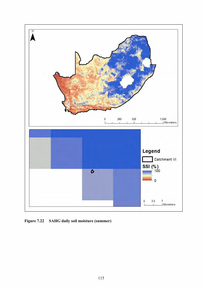
115
Figure 7.22 SAHG daily soil moisture (summer)

116
Figure 7.23 SAHG daily soil moisture (winter)

117
A scatter graph of the CRP (x-axis) was plotted against the SAHG product (y-axis) (Figure
7.24). From Figure 7.24, it can be seen that there is a positive and good correlation between
the datasets. The points are clustered around the 1:1 line (red) and there are no extreme
outliers. There are points below and above the 1:1 line, with the majority of the points being
just below the 1:1 line. The R2 is 0.624, which indicates a close linear relationship between
the datasets. The slope is 1.049, which is close to 1. The points, which are noticeably above
and below the 1:1 line can be attributed to the last three months of the datasets, where there
was less of a correlation between the CRP and SAHG soil moisture estimates. Overall, the
close correlation corresponds to the visual inspection of the data.
Figure 7.24 Scatter graph of CRP against SAHG soil moisture estimates
A graph of the residuals was then plotted against time (Figure 7.25). The ∆ VWC (%) is the
difference between the CRP and SAHG datasets. From Figure 7.25, it is evident that the
majority of the residuals are positive, which indicates that the SAHG soil moisture product
underestimates soil moisture for the majority of the study period. In the dry periods, the
residuals are positive, whilst in the wet periods, there are both positive and negative residuals.
The residuals are generally lower in absolute value in the dry periods, compared to the wet
periods. Once more, the decline in the correlation between the datasets is noticeable between
the first nine months of the study period and the last three months of the study period, which
has the highest residuals with regards to the absolute value of the residuals.
y = 1.0487x - 4.2147R² = 0.6242
0
10
20
30
40
50
60
70
0 10 20 30 40 50 60 70
SAH
G V
WC
(%
)
CRP VWC (%)

118
Figure 7.25 A residual graph of CRP against SAHG was plotted against time
A T-test was conducted. The CRP was variable one and the SAHG product was variable two
(see Table 7.4). From Table 7.4, it can be seen that the means of both variables are similar,
with the CRP mean (33.333) being slightly higher than the SAHG mean (30.742). The
variance of the CRP is 50.292, which is lower than that of the SAHG product (88.607). There
are 677 degrees of freedom. The t stat value is 4.201, which is larger than the t critical two-
tail value of 1.964 and the p value is 3x10-05, which is larger than the alpha value (0.05).
Therefore, according to the T-test, there is a significant difference between the data sets.
Table 7.4 T-test of CRP against SAHG estimates
CRP SAHG Mean 33.333 30.742 Variance 50.292 88.607 Observations 365 365 Hypothesized Mean Difference 0 df 677 t Stat 4.201 P(T<=t) two-tail 3x10-05 t Critical two-tail 1.964
The SAHG soil moisture product provided good estimates of soil moisture, which correlated
well with the CRP estimates. The SAHG soil moisture product measures the SSI (%) in the A
and B soil horizons. In this case, the SSI was obtained at an average depth of one meter.
Therefore, there is a vertical scaling issue, due to the CRP measuring at a depth of around
-25
-20
-15
-10
-5
0
5
10
15
20
25
3/1/2014 5/1/2014 7/1/2014 9/1/2014 11/1/2014 1/1/2015
∆ V
WC
(%)
Date

119
0.12 m, which falls in the range of the SAHG estimate. However, the SAHG product
measures above (0.0 to 0.12 m) and below (0.12 to 1.00 m) and provides an average estimate
of soil moisture. There is a horizontal scaling issue, as the SAHG product is on a 12.5 x 12.5
km spatial grid, which greatly exceeds the measurement footprint of the CRP. For this
research project, all the soil moisture products were converted to volumetric water content
(%), if they were not in volumetric water content (%) already. The SAHG product was in a
SSI and the conversion required an accurate representative porosity value of the study area.
The value determined may not have been the most representative of the study area, but rather
an average of the points selected. This value would result in a constant error throughout the
SAHG volumetric water content dataset.
7.6 SEBS Soil Moisture Validation
In total, 16 relative evaporation and 16 evaporative fraction maps were generated, using the
SEBS Model in ILWIS 3.8.3. These maps were exported, opened and analyzed in ArcGIS
9.3, where the relative evaporation and evaporative fraction of the area within Catchment VI
was determined. The relative evaporation and evaporative fraction values, which were
obtained from the SEBS Model are shown in Table 7.5.
From Table 7.5, it can be seen that the relative evaporation and evaporative fraction results
follow a seasonal trend, as the values are high in summer (wet period) and very low in winter
(dry period), with the intermediate values between the wet and dry periods. Of the 16
estimated relative evaporation and evaporative fraction values, six have high relative
evaporation values (above 0.7), two have intermediate relative evaporation values and eight
have very low relative evaporation values (close to 0).
Catchment VI was burnt on the 5th of September 2014, which could be the reason for the zero
values of the relative evaporation and evaporative fraction being estimated by the SEBS
Model on the 6th of September 2014, 22nd of September 2014 and the 8th of October 2014.
The fire would have resulted in an increase in albedo and a decrease in NDVI, which could
have resulted in these low values. NDVI and albedo are amongst the parameters that the
SEBS Model is most sensitive to (Gibson et al., 2013). A range (high, intermediate and low)
of relative evaporation and evaporative fraction are illustrated in Figure 7.26 and Figure 2.27
respectively.

120
Table 7.5 Relative evaporation and evaporative fraction calculated using the SEBS
model for Catchment VI
Date Relative Evaporation Evaporative Fraction 14-Mar-14 0.73396 0.91684 30-Mar-14 0.94717 0.76871 15-Apr-14 0.87145 0.78335 1-May-14 0.29912 0.50633 17-May-14 Cloud Cloud 2-Jun-14 0.00000 0.00000 18-Jun-14 0.00143 0.00367 4-Jul-14 0.02200 0.04683 20-Jul-14 0.00902 0.01190 5-Aug-14 0.00067 0.00016 21-Aug-14 Cloud Cloud 6-Sep-14 0.00000 0.00000 22-Sep-14 0.00000 0.00000 8-Oct-14 0.00000 0.00000 24-Oct-14 0.11804 0.17727 9-Nov-14 0.93836 0.83581 25-Nov-14 Cloud Cloud 11-Dec-14 0.85773 0.87569 27-Dec-14 Cloud Cloud 12-Jan-15 0.930481 0.94974 28-Jan-15 Cloud Cloud 13-Feb-15 Cloud Cloud
From Figure 7.26, it can be seen that the estimated relative evaporation varies over time. The
30th of March 2014 represents a day when the relative evaporation was very high (0.9471),
the 01st of May represents a day when the relative evaporation was intermediate 0.2991 and
the 05th of August represents a day when the relative evaporation was very low 0.0067.
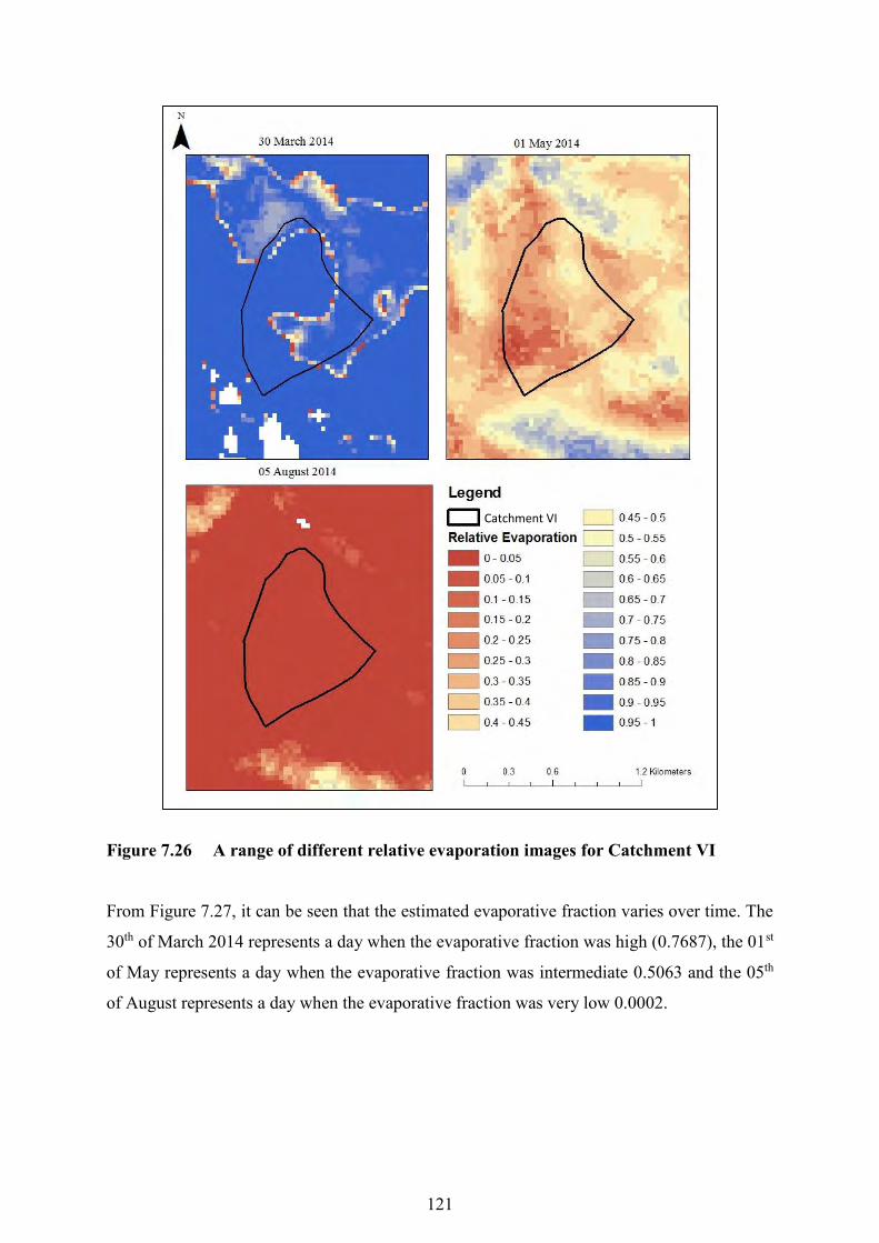
121
Figure 7.26 A range of different relative evaporation images for Catchment VI
From Figure 7.27, it can be seen that the estimated evaporative fraction varies over time. The
30th of March 2014 represents a day when the evaporative fraction was high (0.7687), the 01st
of May represents a day when the evaporative fraction was intermediate 0.5063 and the 05th
of August represents a day when the evaporative fraction was very low 0.0002.
Catchment VI

122
Figure 7.27 A range of different evaporative fraction images
Total evaporation consists of water that is evaporated from the land surface and water that is
transpired from the vegetation. In order to estimate the actual soil moisture, the saturated soil
moisture content is required, which can be inferred from the porosity. The porosity can be
estimated from the bulk density.
The calculation of soil moisture from relative evaporation and evaporative fraction, estimates
the soil moisture in the root zone, from which the evaporated water (soil evaporation,
transpiration and interception) is sourced. The rooting zone of the grassland vegetation is 0.5
Catchment VI

123
m. Therefore, the average bulk density of the soil from 0.0 to 0.5 m is required to obtain the
porosity of the rooting zone. The bulk density was estimated to be 0.688 g/cm3, therefore the
porosity was calculated to be 0.74. This porosity would be used as the saturated soil moisture
content in the rooting zone.
Two methods for soil moisture estimation were investigated in this component of the research
study. The first was developed by Su et al. (2003) and requires the relative evaporation
(Equation 4.12). The second equation was developed by Scott et al. (2003) and requires the
evaporative fraction (Equation 4.13). The estimated soil moisture was plotted against the
corresponding CRP estimates, which were changed to match the 16-day time-step (Figure
7.28).
From Figure 7.28, it can be seen that both methods follow the same trend, as both methods
generally over-estimate soil moisture in the wet period and generally under-estimate soil
moisture in the dry period. Both methods follow a seasonal trend. The Scott et al. (2003)
method seems to perform better, as it over-estimates less in the wet periods, when compared
to the CRP and under-estimates less in the dry period, compared to the CRP, in comparison to
the Su et al. (2003) method.
Figure 7.28 Time series of CRP estimates and soil moisture back-calculated from the
SEBS model
0
10
20
30
40
50
60
70
80
3/1/2014 4/30/2014 6/29/2014 8/28/2014 10/27/2014 12/26/2014 2/24/2015
VW
C (
%)
Date
CRP (daily) CRP (16-day) Su et al., 2003 Scott et al., 2003

124
Scatter graphs of the CRP against Su et al. (2003) and CRP against Scott et al. (2003) were
then plotted (Figure 7.29). From the scatter graphs in Figure 7.29, it can be seen that both
have positive correlations with points above and below the 1:1 line. The points do not cluster
around the 1:1 line. The points above and below the 1:1 indicate over-estimation and under-
estimation of the methods, when compared with the CRP. Both methods have a similar R2
value but different slopes. The (Scott et al., 2003) method has a R2 value of 0.724 and a slope
of 2.819. The (Su et al., 2003) method has a R2 of 0.722 and a slope of 3.862.
Figure 7.29 Scatter graphs of CRP against the SEBS Model estimates a) CRP against
Su et al. (2003) and b) CRP against Scott et al. (2003).
A graph of the residuals for both the CRP against the Scott et al. (2003) method and the CRP
against the Su et al. (2003) method are illustrated in Figure 7.30. From Figure 7.30, both
residuals follow the same trend. The Su et al. (2003) method has greater residuals as it over-
estimates and under-estimates the most in the respective periods, when compared to the CRP
measurements. The Scott et al. (2003) method, resulted in lower absolute valued residuals
than that of Su et al. (2003).
y = 2.8195x - 65.66R² = 0.7238
0
20
40
60
80
0 20 40 60 80
Sco
tt e
t al
. (2
00
3)
VW
C (
%)
CRP VWC (%)
(a)
y = 3.8621x - 98.376R² = 0.7223
0
20
40
60
80
0 20 40 60 80
Su e
t al
. (2
00
3)
VW
C (
%)
CRP VWC (%)
(b)

125
Figure 7.30 Residual graph of CRP against Su et al. (2003) and Scott et al. (2003).
The results show that the method of back-calculating soil moisture, using both equations,
resulted in an over-estimation of soil moisture in the wet periods and an under-estimation of
soil moisture in the dry period. This could be due to either the estimation of the relative
evaporative and the evaporative fraction in the SEBS Model, or the equations used to
calculate soil moisture from the relative evaporative and the evaporative fraction.
The evaporative fraction estimated using the SEBS Model can be validated with an
evaporative fraction calculated from the eddy covariance system, which is situated in
Catchment VI. The relative evaporation cannot be calculated using the eddy covariance
system, as the relative evaporation requires the determination of Hwet (refer to Equations 4.4
and 4.6), which can only be reliably determined through field experiments to determine wet
and dry bulb temperatures. Thus, the following will only look at determining soil moisture
using the Scott et al. (2003) method, as only the evaporative fraction can be determined from
the eddy covariance system.
The eddy covariance with infrared gas analyser measures latent and sensible heat directly.
The eddy covariance system was operational from the 12th of July 2014 to present. The
evaporative fraction was calculated for the same days as the SEBS estimates, using Equation
8.4 (Bastiaanssen et al., 1997):
-40
-30
-20
-10
0
10
20
30
40
3/14/2014 5/14/2014 7/14/2014 9/14/2014 11/14/2014
∆ V
WC
(%)
Date
Su et al. (2003) Scott et al. (2003)

126
ᴧ = 𝐿𝐸
𝐿𝐸+𝐻 (8.4)
where LE is the latent-heat flux and H is the sensible-heat flux. The eddy covariance system
is on a half-hourly time-step. Therefore, a daily relative evaporation value had to be
determined. The evaporative fraction values determined from the SEBS Model and the eddy
covariance system are seen in Table 7.6 below.
Table 7.6 Evaporative fraction estimates from the SEBS Model and eddy covariance
technique
Date SEBS ᴧ EC ᴧ
14-Mar-14 0.91684 -
30-Mar-14 0.76871 -
15-Apr-14 0.78335 -
1-May-14 0.50633 -
2-Jun-14 0.00000 -
18-Jun-14 0.00367 -
4-Jul-14 0.04683 -
20-Jul-14 0.01190 0.17041
5-Aug-14 0.00016 0.21135
6-Sep-14 0.00000 0.14494
22-Sep-14 0.00000 0.26370
8-Oct-14 0.00000 0.46655
24-Oct-14 0.17727 0.62393
9-Nov-14 0.83581 0.73935
11-Dec-14 0.87569 0.70615
12-Jan-15 0.94974 0.75000
The SEBS Model is under-estimating the evaporative fraction in the dry periods and over-
estimating evaporative fraction in the wet periods, as shown in Table 7.6. It is likely that the
SEBS model was the cause of the poor soil moisture results, rather than the two equations
used. The soil moisture was then estimated by using the calculated eddy covariance derived
evaporative fraction in the (Scott et al., 2003) method and plotted with the CRP
measurements against time (see Figure 7.31).
From Figure 7.31, it can be seen that using the evaporative fraction data from the eddy
covariance system, yielded better results of soil moisture, when compared to the CRP
measurements. Using the eddy covariance data in the Scott et al. (2003) method resulted in
an under-estimation of soil moisture in the dry period, but in the wet period, promising soil
moisture estimates were obtained.

127
Figure 7.31 Time series of the CRP soil moisture estimates and soil moisture from the
Scott et al. (2003) method using the evaporative fraction from SEBS and
the eddy covariance method.
When the evaporative fraction of the SEBS Model is compared to the eddy covariance
estimates of evaporative fraction, it is seen that the SEBS model overestimates evaporative
fraction in the wet period, but under-estimates in the dry period. This indicates the limitations
of the SEBS model. The SEBS model was originally created for agriculture, therefore some
model parameterization is not appropriate for non-agricultural land-covers (Gibson et al.,
2013).
The method proposed by Scott et al. (2003) provided better soil moisture results than the
method proposed by Su et al. (2003). This is mainly due to the Su et al. (2003) equation
linking relative soil moisture to relative evaporation by a linear relationship. The use of the
eddy covariance evaporative fraction estimates in the Scott et al. (2003) method, yielded
good results in the wet period. This technique seems promising due to its spatial resolution.
The technique is not limited temporally, but the choice of satellite (Landsat 8) data,
introduces a temporal limitation. This temporal resolution made this method impractical as a
means to monitor soil moisture, as soil moisture is highly variable over time.
0
10
20
30
40
50
60
70
3/1/2014 4/30/2014 6/29/2014 8/28/2014 10/27/2014 12/26/2014
VW
C (
%)
Date
CRP (16-day) EC-Scott et al. (2003) SEBS-Scott et al. (2003)

128
7.7 Evaluating the Satellite-Based Soil Moisture Products
The satellite-based soil moisture products used in this study all have different spatial
resolutions, as seen in Table 7.7. The SEBS back-calculated estimate, obtains soil moisture
on a 0.09 km2 spatial resolution. This resolution is exceptionally small, compared to the other
products and is the only product that has a spatial resolution smaller than the catchment area.
The AMSR2 soil moisture product has the next best spatial resolution, followed by the
SAHG product. The SMOS product has the largest spatial resolution.
Table 7.7 Spatial resolution of soil moisture products
Product Grid (km) Spatial Resolution (km2) AMSR2 10 x 10 100 SMOS 25 x 25 625 SAHG 12.5 x 12.5 156 SEBS 0.3 x 0.3 0.09
The spatial resolution is a key factor in remote sensing, as there is a need to obtain parameter
data on the finest resolution possible. The temporal resolution is just as important, as the need
to continuously monitor parameters is essential. Thus, smaller temporal resolutions are
required. If the observational days of the satellite-based soil moisture products used in this
study are considered, all the products, except for the SAHG product, have days with no data.
The various soil moisture datasets were then compared on their temporal characteristics, over
the one year study period (Figure 7.32).
From Figure 8.32, it can be seen that the SAHG product has a continuous dataset. The
AMSR2 product is a “daily” product, but consists of a few missing days each month, as the
product does not cover the entire surface of the earth each day. The SMOS data, which had
the largest spatial resolution, also had a lot of missing days each month. This was due to the
product not covering the entire earth’s surface each day, as well as missing pixel values
within the covering bands. The SEBS back-calculated product had the fewest observational
days, as it uses Landsat 8 data, which works on a 16-day interval. This results in a maximum
of two images per month. There was a problem with the sensor, which resulted in no
observations in the months of January and February.
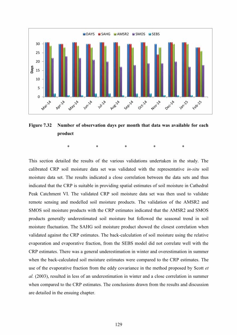
129
Figure 7.32 Number of observation days per month that data was available for each
product
* * * * *
This section detailed the results of the various validations undertaken in the study. The
calibrated CRP soil moisture data set was validated with the representative in-situ soil
moisture data set. The results indicated a close correlation between the data sets and thus
indicated that the CRP is suitable in providing spatial estimates of soil moisture in Cathedral
Peak Catchment VI. The validated CRP soil moisture data set was then used to validate
remote sensing and modelled soil moisture products. The validation of the AMSR2 and
SMOS soil moisture products with the CRP estimates indicated that the AMSR2 and SMOS
products generally underestimated soil moisture but followed the seasonal trend in soil
moisture fluctuation. The SAHG soil moisture product showed the closest correlation when
validated against the CRP estimates. The back-calculation of soil moisture using the relative
evaporation and evaporative fraction, from the SEBS model did not correlate well with the
CRP estimates. There was a general underestimation in winter and overestimation in summer
when the back-calculated soil moisture estimates were compared to the CRP estimates. The
use of the evaporative fraction from the eddy covariance in the method proposed by Scott et
al. (2003), resulted in less of an underestimation in winter and a close correlation in summer
when compared to the CRP estimates. The conclusions drawn from the results and discussion
are detailed in the ensuing chapter.
0
5
10
15
20
25
30
Day
sDAYS SAHG AMSR2 SMOS SEBS

130
8. CONCLUSIONS AND RECOMMENDATIONS
The conclusions and recommendations of the research study are detailed in this chapter.
8.1 Conclusions
Understanding the spatial and temporal variability of soil moisture at different scales is of
great importance in many land surface disciplines, such as hydrology. Soil moisture is a key
hydrological variable, as it impacts the water and energy balance at the land surface-
atmosphere interface and is the main water source for natural vegetation and agriculture. It is
difficult to quantify and assess the soil moisture content at an intermediate scale, due to the
heterogeneity in soil and land cover properties, climate drivers and topography.
The objective of this research study was to compare CRP and satellite-based soil moisture
estimates within Catchment VI of the Cathedral Peak Research Catchments. The three current
methods used to estimate soil moisture were evaluated in this study. These three methods are
in-situ, remote sensing and modelling. Although each method has its own advantages in
measuring soil moisture, they are also greatly limited, as they do not provide soil moisture at
an intermediate scale, which is required for hydrological applications.
The CRP is a new and innovative in-situ instrument that is capable of measuring soil
moisture at an intermediate scale. The CRP, once properly calibrated, is suitable for
providing spatial estimates of soil moisture, as the measurements correlated well with the
representative in-situ soil moisture dataset. The CRP calibration procedure is adequate,
however potential errors can be introduced throughout the procedure, which range from
selecting the sample points, to determining a representative bulk density, to determining the
average neutron count (No) value. Therefore, proper procedure must be adhered to, in order to
minimize potential errors.
The validation of the CRP with a representative catchment soil moisture dataset, from the in-
situ soil moisture network, showed that the CRP is suitable in providing continuous spatial
soil moisture estimates. The in-situ soil moisture dataset could have been more representative

131
of the area, if the echo probes were not destroyed in the fire, however, the remaining in-situ
sensors did create a valuable dataset for the CRP validation.
The calibrated CRP measurements were then used to validate the AMSR2 and SMOS Level
Three soil moisture products. The AMSR2 dataset followed the trend of the CRP and
correlated fairly well, but underestimated soil moisture throughout the study period. The
dataset did have a few missing days. The AMSR2 product was analysed and it was found that
the ascending and descending values correlated well in the dry periods, whilst greater
differences were observed between ascending and descending values in the wet periods.
The SMOS dataset generally under-estimated soil moisture. The dataset did correlate well
and follow the same trend of the CRP. The SMOS dataset had a larger variance and therefore
its values fluctuated more. The dataset had many missing days of data. The SMOS product
was analysed and it was seen that the ascending and descending values were different
throughout. The key issue in the validation of the AMSR2 and SMOS soil moisture products
with the CRP measurements, is the vertical and horizontal scaling issue. Although the CRP is
an improvement from validating remote sensing products with in-situ point measurements,
the difference in measurement depths and the footprint of the CRP and current remote soil
moisture products still remain a limitation.
The AMSR2 and SMOS products consist of ascending and descending values. It has been
shown that there were differences in these values, which could be attributed to changes in soil
moisture in the 12-hour interval between ascending and descending acquisition. It was noted
that there were also differences in day and night geo-physical conditions, with nocturnal
conditions being more favourable for soil moisture retrieval from AMSR2 and SMOS
products.
The CRP was then used to validate modeled soil moisture estimates. These included the
SAHG soil moisture product and the back-calculation of soil moisture from relative
evaporation estimated from the SEBS Model.
The SAHG soil moisture product was validated with the CRP. There was a close correlation
between the SAHG and CRP datasets. The SAHG soil moisture followed the same seasonal
trend as the CRP and had a continuous dataset (no missing values). The SAHG product
generally had a slight underestimation of soil moisture. Although the SAHG product

132
performed well, there was still the presence of vertical and horizontal scaling issues, due to
differences in the measurement depth and footprint of the two datasets. There is also the issue
of the conversion of the SSI to VWC, which required a representative porosity of the study
area to be determined.
The back-calculation of soil moisture from relative evaporation and evaporative fraction,
estimated using the SEBS model, looked like a promising technique. The spatial resolution
was less than the catchment area and the measurement depth was representative of the root
zone of the vegetation (0.50 m). Therefore, this product would have the least horizontal and
vertical scaling issues, when validated against the CRP. The SEBS model did not provide
accurate estimates of relative evaporation and evaporative fraction compared to the
evaporative fraction estimates from the eddy covariance system. The SEBS Model over-
estimated the evaporative fraction in the wet period, whilst under-estimating the evaporative
fraction in the dry periods, which resulted in soil moisture over-estimation in the wet periods
and under-estimation in the dry periods. When the evaporative fraction derived from the eddy
covariance system was used in the (Scott et al., 2003) method, the resultant soil moisture
estimates, under-estimated in the dry period, however promising estimates were obtained in
the wet period, which correlated well with the CRP estimates. Although the back-calculation
method results in soil moisture estimates on a 30 m spatial grid, the temporal resolution of the
imagery used is 16 days, which is very impractical for continuous soil moisture monitoring.
8.2 Recommendations
The following recommendations can be used to address the main limitations that were
experienced in this research study. This will provide assistance for future research studies.
i. The calibration of the CRP is both time and labour intensive, as calibrations over
different periods are required. There are a variety of errors that could emerge
throughout the calibration procedure. Therefore, the proper techniques and
equipment must be used to minimize the occurrence of errors, in order to obtain
reliable soil moisture measurements. The use of a TDR HydroSense probe, which
obtains instantaneous measurements of soil moisture, when inserted into the soil, can
potentially be used to obtain the necessary soil moisture measurements for the
calibration. Thus, it would greatly reduce the time and labour required.

133
ii. The validation of the CRP needs to be done with in-situ soil moisture sensors at a
variety of depths. Ideally several TDR pits, in the CRP measurement volume could
be used. This would improve the validation, as the CRP doesn’t measure at a constant
depth and therefore, shouldn’t be validated with in-situ measurements at a constant
depth. However, this would be very capital, time and labour intensive.
iii. The potential for using temporal stability analysis to find a more representative
sensor location would be useful to upscale the in-situ observations to the entire
catchment.
iv. Current remote sensing soil moisture products are still too coarse to be validated with
CRP measurements. Although the use of the CRP for the validation of remote
sensing soil moisture products is an improvement, the vertical and horizontal scaling
issues still remain as major limitations. This limitation could potentially be addressed
through the downscaling of remote sensing soil moisture products, in order to obtain
finer spatial scale soil moisture estimates.
v. The back-calculation of soil moisture using relative evaporation and evaporated
fraction, from the SEBS Model, indicated that the use of the SEBS Model is not
suitable in the study area for the estimation of these parameters. Future research
should limit the use the SEBS model to agricultural landscapes.

134
9. REFERENCES
Albergel, C, de Rosnay, P, Gruhier, C, Mu˜noz-Sabater, J, Hasenauer, S, Isaksen, L, Kerr, Y
and Wagner, W. 2012. Evaluation of remotely sensed and modelled soil moisture
products using global ground-based in situ observations. Remote Sens. Environ 118:
215-226.
Allen, R, Bastiaanssen, W and Waters, R. 2002. Personal communication, the University of
Idaho and the Idaho Department of Water Resources, The University of Idaho,
Bastiaanssen, W, Pelgrum, H, Droogers, P, de Bruin, H and Menenti, M. 1997. Area-average
estimates of evaporation, wetness indicators and top soil moisture during two golden
days in EFEDA. Agric Forest Meteorol 87: 119-137.
Bezerra, B, dos Santos, C, da Silva, B, Bezerra, M, Bezerra, J and Rao, T. 2013. Estimation
of soil moisture in the root-zone from remote sensing data. . Ci. Solo 37: 596-603.
Brocca, L, Hasenauer, S, Lacava, T, Melone, F, Moramarco, T, Wagner, W, Dorigo, W and
Bittelli, M. 2011. Soil moisture estimation through ASCAT and AMSR-E sensors: An
intercomparison and validation study across Europe. Remote Sensing of Environment
115: 3390-3408.
Brocca, L, Tarpanelli, A, Moramarco, T, Melone, F, Ratto, S, Cauduro, M, Ferraris, S, Berni,
N, Ponziani, F, Wagner, W and Melzer, T. 2013. Soil moisture estimation in Alpine
Catchments through modeling and satellite observations. Soil Science Society of
America
Desilets, D and Zreda, M. 2013. Footprint diameter for a cosmic-ray soil moisture probe:
theory and Monte Carlo simulations. Water Resources Research 49: 3566-3575.
Desilets, D, Zreda, M and Ferre, T. 2010. Nature’s neutron probe: land surface hydrology at
an elusive scale with cosmic rays. Water Resources Research 46: 1-7.
Dorigo, W, Wagner, W, Hohensinn, H, Paulik, C, Xaver, A and Jackson, T. 2011. The
International Soil Moisture Network: A data hosting facility for global in situ soil
moisture measurements. Hydrology and Earth System Sciences. Hydrol. Earth Syst.
Sci 15: 1675-1698.
Draper, CS, Walker, JP, Steinhle, P and Holmes, TRH. 2009. An evaluation of AMSR–E
derived soil moisture over Australia. Remote Sensing of Environment 113 (4): 703-
710.

135
Dutta, R and D'este, C. 2013. Virtual Calibration of Cosmic Ray Sensor: using supervised
ensemble machine Learning. IJACSA) International Journal of Advanced Computer
Science and Applications 4: (8): 104-110.
Engman, ET. 1991. Application of microwave remote sensing of soil moisture for water
resources and agriculture. Remote Sensing of Environment 35: 213-226.
Everson, CS, Molefe, GL and Everson, TM. 1998. Monitoring and modelling components of
the water balance in a grassland catchment in the summer rainfall area of South
Africa.
Fang, B and Lakshmi, V. 2014. Soil moisture at watershed scale : Remote sensing techniques
Journal of Hydrology 516: 258-272.
Franz, T. 2014. Personal communication, Franz Hydrogeophysics Lab Group, 1-4.,
Franz, T, Wang, T, Avery, W, Finkenbiner, C and Brocca, L. 2015. Spatiotemporal
characterization of soil moisture fields in agricultural areas using cosmic-ray neutron
probes and data fusion. EGU General Assembly 17
Franz, T, Zreda, M, Ferre, T and Rosolem, R. 2013. An assessment of the effect of horizontal
soil moisture heterogeneity on the area-average measurement of cosmic-ray neutrons.
Water Resources Research 49: 1-9.
Franz, T, Zreda, M, Rosolem, R and Ferre, T. 2012a. Field Validation of a cosmic-ray
neutron sensor using a distributed sensor network. Vadose Zone Journal 11
Franz, T, Zreda, M, Rosolem, R and Ferre, T. 2012b. A universal calibration function for
determination of soil moisture with cosmic-ray neutrons. Hydrology and Earth System
Sciences Discussions 9: 10303-10322.
Gibson, L, Jarmain, C, Su, Z and Eckardt, F. 2013. Estimating evapotranspiration using
remote sensing and the Surface Energy Balance System - A South African
Perspective. Water SA 39: 477-484.
Gokman, M, Vekerdy, Z, Verhoef, A, Verhoef, W, Batelaan, O and van der Tol, C. 2012.
Integration of soil moisture in SEBS for improving evapotranspiration estimation
under water stress conditions. Remote Sensing of Environment 121: 261-274.
Gruber, A, Dorigo, WA, Zwieback, S, Xaver, A and Wagner, W. 2013. Characterizing
coarse-scale representativeness of in situ soil moisture measurements from the
International soil moisture network. gsvadzone 12 (2):
Gruhier, C, Albergel, C, de Rosnay, P and Zeiner, B. 2011. Comparison between H-SAF
large scale surface soil moisture, H-SAF assimilated soil moisture and SMOS Level 2
soil moisture. CESBIO, Toulouse, France.

136
Guillem, M. 2010. Multi-scale soil moisture retrievals from microwave remote sensing
observations. Unpublished thesis, Remote Sensing Lab, Dept. Teoria del Senyal I
Comunicacions Universitat Polit Ecnica de Catalunya,
Gush, M, Scott, DF, Jewitt, GPW, Schulze, RE, Lumsden, T, Hallowes, L and Gorgens, A.
2002. Estimation of streamflow reduction resulting from commercial afforestation in
South Africa.
Hawdon, A, Mcjannet, D and Wallace, J. 2014. Calibration and correction procedures for
cosmic-ray neutron soil moisture probes located across Australia. Water Resources
Research 50 (6): 5029-5043.
Hillel, D. 2008. In: ed. Hillel, D, Soil in the Environment. Academic Press, San Diego.
Imaoka, K, Kachi, M, Kasahara, M, Ito, N, Nakagawa, K and Oki, T. 2010. Instrument
performance and calibration of AMSR-E and AMSR2. International Archives of the
Photogrammetry, Remote Sensing and Spatial Infromation Science 38: 13-16.
Jackson, TJ, Cosh, MH, Bindlish, R, Starks, PJ, Bosch, DD, Seyfried, M, Goodrich, DC,
Moran, MS and Du, J. 2010. Validation of advanced microwave scanning radiometer
soil moisture products. IEEE Transactions on Geoscience and Remote Sensing 48
(12):
Jarmain, C, Govender, M and Everson, CS. 2004. Improving the basis for predicting total
evaporation from natural veld types in South Africa.
JAXA, JAEA. 2013a. AMSR Level 3 Product Format Description Document.
JAXA, JAEA. 2013b. GCOM-W1 "SHIZUKU" Data Users Handbook. First Edition.
Jiao, Q, Zhu, Z and Du, F. 2014. Theory and application of measuring mesoscale soil
moisture by cosmic-ray fast neutron probe. 35th International Symposium on Remote
Sensing of Environment 17
Jones, SB, Wraith, JM and Or, D. 2002. Time domain reflectometry measurement principles
and applications. Hydrological Processes 16: 141-153.
Kerr, YH, Waldteufel, P, Richaume, P, Wigneron, JP, Ferrazzoli, P, Mahmoodi, A, Al Bitar,
A, Cabot, F, Gruhier, C, Juglea, SE, Leroux, D, Mialon, A and Delwart, S. 2012. The
SMOS soil moisture retrieval algorithm. Geoscience and Remote Sensing, IEEE
Transactions on 50 (5): 1384-1403.
Kerr, YH, Waldteufel, P, Wigneron, JP, Delwart, S, Cabot, F, Boutin, J, Escorihuela, MJ,
Font, J, Reul, N, Gruhier, C, Juglea, SE, Drinkwater, MR, Neira, M and Mecklenburg,
S. 2010. The SMOS mission: new tool for monitoring key elements of the global
water cycle. Proceedings of the IEEE 98 (5): 666-687.

137
Kim, S, Liu, YY, Johnson, FM, Parinussa, RM and Sharma, A. 2015. A global comparison of
alternate AMSR2 soil moisture products: Why do they differ ? Remote Sensing of
Environment
Kohli, M, Shron, M, Zreda, M, Schmidt, U, Dietrich, P and Zacharias, S. 2015. Footprint
characteristics revised for field-scale soil moisture monitoring with cosmic-ray
neutrons. Water Resources Research 10: 5772-5790.
Koike, T, Nakamura, YK and Fujii, I. 2004. Development of an Advanced Microwave
Scanning Radiometer (AMSR-E) Algorithm of soil moisture and vegetation water
content. Annual Journal of Hydraulic Engineering 48 (2): 217-222.
Kuenene, BT, van Huyssteen, CW and Hensley, M. 2009. Soil water saturation in the
Cathedral Peak VI catchment, KwaZulu-Natal. SAGA Biennial Technical Meeting and
Exhibition 11: 565-570.
Lakshmi, V. 2013. Remote sensing of soil moisture. ISRN Soil Science 2013: 33 pages.
Leroux, D, Kerr, YH, Al Bitar, A, Bindlish, R, Jackson, TJ, Berthelot, N and Portet, G. 2013.
Comparison between SMOS, VUA, ASCAT and ECMWF soil moisture products
over four watersheds in United States. IEEE Transactions on Geoscience and Remote
Sensing 1-20.
Lu, H, Koike, T and Yang, K. 2014. Improvement of AMSR2 soil moisture algorithm with
considering temperature profile effects in dry soil: a case study in Heihe Basin. IEEE
3299-3302.
Ma, W, Hafeez, M, Rabbani, U, Ishikawa, H and Ma, Y. 2012. Retrieved actual ET using
SEBS model from Landsat-5 TM data for irrigation area of Australia. Atmospheric
Environment 59: 408-414.
Markham, B, Storey, J and Morfitt, R. 2015. Landsat-8 sensor characterization and
calibration. Remote Sens 2015 (7): 2279-2282.
Mecklenburg, S, Drusch, M, Kerr, Y, Font, J and Roger, O. 2013. ESA’s soil moisture and
ocean salinity mission: mission performance and operations. European Space Agency,
ESA-ESRIN, Via Galileo Galilei, Frascati, Italy.
Mekonnen, D. 2009. Satellite remote sensing for soil moisture estimation: Gumara
catchment, Ethiopia. Unpublished thesis, International institute for geo-information
science and earth observation, Netherlands.
Meng, L and Quiring, SM. 2008. A Comparison of Soil Moisture Models Using Soil Climate
Analysis Network Observations. American Meteorological Society 9: 641-659.
138
Mengistu, MG, Everson, CS, Moyo, NC and Savage, MJ. 2014. The validation of the
variables (evaporation and soil moisture) in hydrometeorological models.
Merlin, O, Al Bitar, A, Walker, JP and Kerr, Y. 2009. A sequential model for disaggregating
near-surface soil moisture observations using multi-resolution thermal sensors.
Remote Sensing of Environment 113 (10): 2275-2284.
Merlin, O, Al Bitar, A, Walker, JP and Kerr, Y. 2010. An improved algorithm for
disaggregating microwave-derived soil moisture based on red, near-infrared and
thermal-infrared data. Remote Sensing of Environment 114 (10): 2305-2316.
Merlin, O, Rudiger, C, Al Bitar, A, Richaume, P, Walker, JP and Kerr, YH. 2012.
Disaggregation of SMOS soil moisture in southeastern Australia. Geoscience and
Remote Sensing, IEEE Transactions on 50 (5): 1556-1571.
Merlin, O, Walker, JP, Chehbouni, A and Kerr, Y. 2008. Towards deterministic downscaling
of SMOS soil moisture using MODIS derived soil evaporative efficiency. Remote
Sensing of Environment 112 (10): 3935-3946.
Ni-Meister, W. 2005. Soil moisture initialization for climate prediction: characterization of
model and observation errors. Journal of Geophysical Research 110: 11-29.
Ochsner, TE, Cosh, MH, Cuenca, RH, Dorigo, WA, Draper, CS, Hagimoto, Y, Kerr, YH,
Larson, KM, Njoku, EG, Small, EE and Zreda, M. 2013. State of the art in large-scale
soil moisture monitoring. . Soil Science Society of America.
Parrens, M, Zakharova, E, Lafont, S, Calvet, JC, Kerr, YH, Wagner, W and Wigeron, JP.
2012. Comparing soil moisture retrievals from SMOS and ASCAT over France.
Hydrol. Earth Syst. Sci 16: 423-440.
Piles, M, Camps, A, Vall-llossera, M, Corbella, I, Panciera, R, Rudiger, C, Kerr, YH and
Walker, JP. 2011. Downscaling SMOS-derived soil moisture using MODIS
visible/infrared Data. IEEE Transactions on Geoscience and Remote Sensing 49 (9):
Qin, J, Yang, K, Chen, Y, Zhao, L and Han, M. 2013. Spatial up-scaling of in-situ soil
moisture measurements based on MODIS-derived apparent thermal inertia. Remote
Sensing of Environment 138: 1-9.
Sabins, FF. 2007. Remote Sensing Principles and Interpretation. Waveland Press, Illinois.
Scott, C, Bastiaanssen, W and Ahmad, M. 2003. Mapping spatio-temporal distributions of
soil moisture throughout irrigated watersheds using optical and high resolution
imagery. ASCE Irrigat and Drain Eng 129
Scott, DF. 1994. The hydrological effects of fire in South African catchments. . Unpublished
thesis, Department of Agricutural Engineering, University of Natal, South Africa,
139
Scott, DF, Prinsloo, FW, Moses, G, Mehlomakulu, M and Simmers, ADA. 2000. A re-
analysis of the South African catchment afforestation experimental data
Shin, Y and Mohanty, BP. 2013. Development of a deterministic downscaling algorithm for
remote sensing soil moisture footprint using soil and vegetation classifications. Water
Resources Research 49: 6208-6228.
Sinclair, S and Pegram, GGS. 2010. A comparison of ASCAT and modeled soil moisture
over South Africa, using TOPKAPI in land surface mode. Hydrol. Earth Syst. Sci. 14:
613-626.
Sinclair, S and Pegram, GGS. 2012. PyTOPKAPI – an open-source implementation of the
TOPKAPI hydrological model. Pegram and Associates.
Sinclair, S and Pegram, GGS. 2013a. HYLARSMET: A hydrologically consistent land surface
model for soil moisture and evapotranspiration modelling over Southern Africa using
remote sensing and meteorological data.
Sinclair, S and Pegram, GGS. 2013b. A sensitivity assessment of the TOPKAPI model with
an added infiltration module. Journal of Hydrology 479: 100-112.
Song, C, Jia, L and Menenti, M. 2013. Retrieving high-resolution surface soil moisture by
downscaling AMSR-E brightness temperature using MODIS LST and NDVI data.
IEEE Journal of Selected Topics in Applied Earth Observations and Remote Sensing
(2013): 1939-1404.
Stoof, CR, Vervoort, RW, Iwema, J, van de Elsen, E, Ferreira, AJD and Ritsema, CJ. 2012.
Hydrological response of a small catchment burned by experimental fire. Hydrol.
Earth Syst. Sci 16: 267-285.
Su, Z. 2002. The Surface Energy Balance System (SEBS) for estimation of turbulent heat
fluxes. Hydrology and Earth System Sciences 6: 85-99.
Su, Z, Yacob, A, Wen, J, Roerink, G, He, Y, Gao, B, Boogaard, H and van Diepen, C. 2003.
Assessing relative soil moisture with remote sensing data: theory, experimental
validation, and application to drought monitoring over the North China Plain. Physics
and Chemistry of the Earth 28: 89-101.
USGS. 2013. Using the USGS Landsat 8 Product. [Internet]. Available from:
http://landsat.usgs.gov/Landsat8_Using_Product.php. [Accessed: February].
USGS. 2015. Landsat 8 (L8) data users handbook
Villarreyes, CAR, Baroni, G and Oswald, SE. 2013. Calibration approaches of cosmic-ray
neutron sensing for soil moisture measurement in cropped fields. Hydrology and
Earth System Sciences 10: 4237-4274.

140
Vischel, T, Pegram, GGS, Sinclair, S and Parak, M. 2008. Implementation of the TOPKAPI
model in South Africa: initial results from the Liebenbergsvlei catchment. Water SA
34 (3): 1-12.
Wagner, W. 2008. Remote sensing of soil moisture in support to hydrological and
meteorological modelling. METIER Training Course "Remote Sensing of the
Hydrosphere" Finish Environment Institute, Helsinki, Finland.
Wagner, W, Dorigo, W, de Jeu, R and Fernandez, JC. 2012. Fusion of active and passive
microwave observations to create an essential climate variable data record on soil
moisture. Vienna University of Technology, Institute of Photogrammetry and Remote
Sensing, Gusshausstrasse, 1040 Wien, Austria.
Walker, JP, Willgoose, GR and Kalma, JD. 2004. In situ measurement of soil moisture: a
comparison of techniques. Journal of Hydrology 2963: 85-99.
Wang, L and Qu, J. 2009. Satellite of remote sensing application for surface soil moisture
monitoring. Front. Earth Sci. 3 (2): 237-247.
Zazueta, FS and Xin, J. 1994. Soil Moisture Sensors. University of Florida.
Zhang, A, Jia, G, Wang, S, Zhoa, TB and Feng, JM. 2011. Evaluation of AMSR-E derived
soil moisture over Northern China. China. Atmospheric and Oceanic Science. 4 (4):
223-228.
Zhao, W and Li, A. 2013. A downscaling method for improving the spatial resolution of
AMSR-E derived soil moisture product based on MSG-SEVIRI data. Remote Sensing
of Environment 5 (2013): 6790-6811.
Zreda, M, Desilets, D, Ferre, TPA and Scott, RL. 2008. Measuring soil moisture content non-
invasively at intermediate spatial scale using cosmic-ray neutrons. Geophysical
Research 35
Zreda, M, Shuttleworth, WJ, Zeng, X, Zweck, C, Desilets, D, Franz, T and Rosolem, R.
2012. COSMOS: the COsmic-ray Soil Moisture Observing System. Hydrol. Earth
Syst. Sci. 16: 4079-4099.